This article was downloaded by: [West Virginia University]On: 05 November 2012, At: 08:20Publisher: Taylor & FrancisInforma Ltd Registered in England and Wales Registered Number: 1072954 Registeredoffice: Mortimer House, 37-41 Mortimer Street, London W1T 3JH, UK

International Journal of RemoteSensingPublication details, including instructions for authors andsubscription information:http://www.tandfonline.com/loi/tres20

Does spatial resolution matter? A multi-scale comparison of object-based andpixel-based methods for detectingchange associated with gas well drillingoperationsBenjamin A. Baker a , Timothy A. Warner a , Jamison F. Conley a &Brenden E. McNeil aa Department of Geology and Geography, West Virginia University,Morgantown, WV, 26506-6300, USAVersion of record first published: 31 Oct 2012.

To cite this article: Benjamin A. Baker, Timothy A. Warner, Jamison F. Conley & Brenden E. McNeil(2013): Does spatial resolution matter? A multi-scale comparison of object-based and pixel-basedmethods for detecting change associated with gas well drilling operations, International Journal ofRemote Sensing, 34:5, 1633-1651

To link to this article: http://dx.doi.org/10.1080/01431161.2012.724540

PLEASE SCROLL DOWN FOR ARTICLE

Full terms and conditions of use: http://www.tandfonline.com/page/terms-and-conditions

This article may be used for research, teaching, and private study purposes. Anysubstantial or systematic reproduction, redistribution, reselling, loan, sub-licensing,systematic supply, or distribution in any form to anyone is expressly forbidden.

The publisher does not give any warranty express or implied or make any representationthat the contents will be complete or accurate or up to date. The accuracy of anyinstructions, formulae, and drug doses should be independently verified with primarysources. The publisher shall not be liable for any loss, actions, claims, proceedings,demand, or costs or damages whatsoever or howsoever caused arising directly orindirectly in connection with or arising out of the use of this material.

International Journal of Remote SensingVol. 34, No. 5, 10 March 2013, 1633–1651

Does spatial resolution matter? A multi-scale comparisonof object-based and pixel-based methods for detecting change

associated with gas well drilling operations

Benjamin A. Baker, Timothy A. Warner*, Jamison F. Conley, and Brenden E. McNeil

Department of Geology and Geography, West Virginia University, Morgantown, WV26506-6300, USA

(Received 25 May 2012; accepted 30 July 2012)

An implicit assumption of the geographic object-based image analysis (GEOBIA)literature is that GEOBIA is more accurate than pixel-based methods for high spa-tial resolution image classification, but that the benefits of using GEOBIA are likelyto be lower when moderate resolution data are employed. This study investigates thisassumption within the context of a case study of mapping forest clearings associatedwith drilling for natural gas. The forest clearings varied from 0.2 to 9.2 ha, with anaverage size of 0.9 ha. National Aerial Imagery Program data from 2004 to 2010, with1 m pixel size, were resampled through pixel aggregation to generate imagery with2, 5, 15, and 30 m pixel sizes. The imagery for each date and at each of the five spa-tial resolutions was classified into Forest and Non-forest classes, using both maximumlikelihood and GEOBIA. Change maps were generated through overlay of the classi-fied images. Accuracy evaluation was carried out using a random sampling approach.The 1 m GEOBIA classification was found to be significantly more accurate than theGEOBIA and per-pixel classifications with either 15 or 30 m resolution. However, atany one particular pixel size (e.g. 1 m), the pixel-based classification was not statis-tically different from the GEOBIA classification. In addition, for the specific class offorest clearings, accuracy varied with the spatial resolution of the imagery. As the pixelsize coarsened from 1 to 30 m, accuracy for the per-pixel method increased from 59%to 80%, but decreased from 71% to 58% for the GEOBIA classification. In summary,for studying the impact of forest clearing associated with gas extraction, GEOBIA ismore accurate than pixel-based methods, but only at the very finest resolution of 1 m.For coarser spatial resolutions, per-pixel methods are not statistically different fromGEOBIA.

1. Introduction

Geographic object-based image analysis (GEOBIA, also commonly known as object-basedimage analysis (OBIA); Hay and Castilla 2008; Blaschke 2010) has become an increasingfocus of the remote-sensing community, especially in the past decade. This rising interestin GEOBIA is usually ascribed, at least in part, to the advent of commercial fine spatialresolution (with a pixel size less than 10 m) satellite imagery (Blaschke et al. 2000; Hayand Castilla 2008). Fine spatial resolution imagery is assumed to have high local variabilityin pixel digital numbers (DNs). Consequently, analysis and classification that is based on

*Corresponding author. Email: Tim.Warner@mail.wvu.edu

ISSN 0143-1161 print/ISSN 1366-5901 online© 2013 Taylor & Francishttp://dx.doi.org/10.1080/01431161.2012.724540http://www.tandfonline.com

Dow

nloa

ded

by [

Wes

t Vir

gini

a U

nive

rsity

] at

08:

20 0

5 N

ovem

ber

2012

1634 B.A. Baker et al.

contiguous groups of pixels, termed image objects (or just objects, for short), is assumedto be more effective than one based on individual pixels, since the objects effectively sup-press this local variability in the final map product (Johansen et al. 2010; Kim et al. 2011;Malinverni et al. 2011). In moderate spatial resolution images (10–100 m), the individualpixels are expected to contain multiple ground objects, and therefore GEOBIA is regardedas less useful for such images (Blaschke 2010). Thus, for example, Giner and Rogan (2012)used GEOBIA for high spatial resolution aerial imagery, but pixel unmixing methodsfor Landsat images. Nevertheless, a number of studies have found GEOBIA-based meth-ods effective for classification of moderate resolution imagery (e.g. Matinfar et al. 2007;Gamanya, De Maeyer, and De Dapper 2009). Notably, however, comparisons betweenpixel- and object-based methods using fine resolution imagery generally find object-basedmethods more accurate (e.g. Platt and Rapoza 2008; Pringle et al. 2009), but at moderateresolutions the relative benefits are less clear. For example, Robertson and King (2011),using 30 m Landsat Thematic Mapper (TM) data, found no significant difference betweenthe two approaches, although when the classifications were used for change detection, theyfound some evidence that object-based methods were more accurate. Dorren, Maier, andSeijmonsbergen (2003) found that pixel-based methods of forest classification were moreaccurate statistically, but they also noted that local foresters evaluated the object-basedmaps as being a better representation of the change.

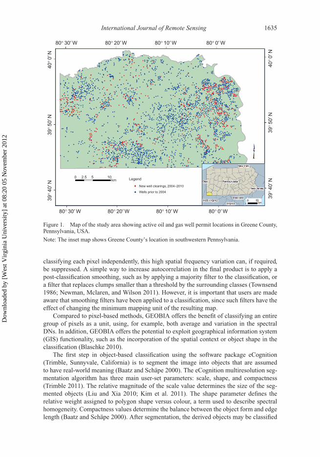
The focus on high spatial resolution as a driver of GEOBIA development, and theambiguous findings in previous studies regarding GEOBIA with moderate resolutionimagery, raises the question whether GEOBIA is inherently more accurate at fine spatialresolutions than moderate resolutions, and how both pixel-based and object-based meth-ods compare in relative accuracy as a function of spatial resolution. (For simplicity sake,we use ‘scale’ to refer to spatial resolution, although it is important to bear in mind thatimage scale has additional components (Warner, Nellis, and Foody 2009b).) The issues ofscale and GEOBIA classification are addressed in this article within the context of the iden-tification of recent, rapid, and spatially extensive land-cover change associated with forestclearing for natural gas well drilling sites in the central Appalachian Plateaus physiographicprovince, USA (Fenneman 1917) (Figure 1). Although the clearings within the study siteare relatively small (averaging 0.9 ha, with a range in size from 0.2 to 9.2 ha), the largenumber and dispersed locations suggest that the cumulative effect, especially in terms offorest fragmentation, may be great. The primary data set was aerial imagery with a pixelsize of 1 m, from which additional spatial scales from 2 to 30 m were synthesized. Manypapers have examined the role of the scale of the objects in GEOBIA (e.g. Kim, Madden,and Warner 2009; Liu and Xia 2010; Dragut and Eisank 2011), but to our knowledge this isthe first paper to methodically examine the effect of the scale of the pixels used to generatethe objects.

2. GEOBIA, classification, and change detection

Traditional, aspatial classification methods analyse remotely sensed imagery on a pixel-by-pixel basis, irrespective of the decisions made for neighbouring pixels (Jensen et al.2009). Maximum likelihood classification is one of the most common pixel-based classi-fication methods because of its ‘simplicity and robustness’ (Platt and Goetz 2004, 816).Maximum likelihood classification assigns pixels to a land-cover class based upon themaximum probability a pixel belongs to one of a number of classes provided by theuser as training samples. Although pixel-based classifications such as maximum likelihoodclassification are often criticized for the ‘salt and pepper effect’, which is a consequence of

Dow

nloa

ded

by [

Wes

t Vir

gini

a U

nive

rsity

] at

08:

20 0

5 N

ovem

ber

2012

International Journal of Remote Sensing 1635

80° 20′ W 80° 0′ W80° 10′ W80° 30′ W

80° 20′ W 80° 0′ W80° 10′ W80° 30′ W

40° 0

′ N39

° 40′

N39

° 50′

N

40° 0

′ N39

° 40′

N39

° 50′

N

0km

10

New well clearings, 2004–2010

Wells prior to 2004

Legend52.5

Figure 1. Map of the study area showing active oil and gas well permit locations in Greene County,Pennsylvania, USA.

Note: The inset map shows Greene County’s location in southwestern Pennsylvania.

classifying each pixel independently, this high spatial frequency variation can, if required,be suppressed. A simple way to increase autocorrelation in the final product is to apply apost-classification smoothing, such as by applying a majority filter to the classification, ora filter that replaces clumps smaller than a threshold by the surrounding classes (Townsend1986; Newman, Mclaren, and Wilson 2011). However, it is important that users are madeaware that smoothing filters have been applied to a classification, since such filters have theeffect of changing the minimum mapping unit of the resulting map.

Compared to pixel-based methods, GEOBIA offers the benefit of classifying an entiregroup of pixels as a unit, using, for example, both average and variation in the spectralDNs. In addition, GEOBIA offers the potential to exploit geographical information system(GIS) functionality, such as the incorporation of the spatial context or object shape in theclassification (Blaschke 2010).

The first step in object-based classification using the software package eCognition(Trimble, Sunnyvale, California) is to segment the image into objects that are assumedto have real-world meaning (Baatz and Schäpe 2000). The eCognition multiresolution seg-mentation algorithm has three main user-set parameters: scale, shape, and compactness(Trimble 2011). The relative magnitude of the scale value determines the size of the seg-mented objects (Liu and Xia 2010; Kim et al. 2011). The shape parameter defines therelative weight assigned to polygon shape versus colour, a term used to describe spectralhomogeneity. Compactness values determine the balance between the object form and edgelength (Baatz and Schäpe 2000). After segmentation, the derived objects may be classified

Dow

nloa

ded

by [

Wes

t Vir

gini

a U

nive

rsity

] at

08:

20 0

5 N

ovem

ber

2012

1636 B.A. Baker et al.

using textural, spectral, and other properties of the object specified by the user (Trimble2011). Two approaches that are commonly used with eCognition are the membership func-tion classifier and the nearest neighbour classifier. The membership function classifierrequires an expert to create rules for classifying objects, whereas the nearest neighbourclassifier requires training objects for each class (Myint et al. 2011).

Change detection using remotely sensed imagery has proved to be useful in a widerange of natural resource extraction studies, especially in surface mining (e.g. Townsendet al. 2009) and logging (e.g. Franklin et al. 2002). As with image classification, changedetection methods include both pixel-based and GEOBIA methods (Warner, Almutairi,and Lee 2009a). A common pixel-based method for observing land-cover change ispost-classification change detection. This method of change detection uses independentlyclassified thematic maps followed by a GIS overlay to assess land-cover change betweenthe classifications (Jensen 2005). Post-classification change detection is regarded as one ofthe simplest approaches to change detection studies because atmospheric correction is notrequired (Warner, Almutairi, and Lee 2009a). However, one of the major criticisms of thisapproach is that the error of the change analysis can be, at least in the worst case, the prod-uct of errors of the independent classifications (Singh 1989; van Oort 2007). Furthermore,as with all pixel-based methods, a precise co-registration between the images of differentdates is essential (Dai and Khorram 1998).

Whereas pixel-based change detection is limited to change of individual pixels,GEOBIA change detection has the potential to address some of the challenges of traditionalmethods. Because it produces homogeneous objects, GEOBIA change detection does notsuffer from spatially uncorrelated salt-and-pepper noise in the change products. On theother hand, GEOBIA change detection is very sensitive to the locations of the delineatedobject boundaries. Slight changes in object delineation between the different dates due todifferences in image co-registration, sun-angle, or even just natural variation in image DNswill result in spurious identification of change along the object boundaries (Gamanya, DeMaeyer, and De Dapper 2009).

Post-classification GEOBIA change detection is based upon three steps. First, theimages are segmented into image objects (Blaschke 2010). These objects are then clas-sified into land-cover categories (Gamanya, De Maeyer, and De Dapper 2009; Myint et al.2011), and then in the final stage the change is mapped. Ideally, change would be identifiedon an object basis (Gamanya, De Maeyer, and De Dapper 2009; Chen et al. 2012). A sim-ple alternative to the complexities of an object-based approach is to apply a raster GISoverlay of the GEOBIA classifications, ignoring the object relationships. The disadvantageof this approach is that changes to specific objects are lost. However, in cases where indi-vidual objects are not of interest, this strategy provides an effective method for assessingland-cover change.

3. Study area and data

The study area for this research is Greene County, located in the southwestern cornerof Pennsylvania and bordered on the west and south by West Virginia (Figure 1). Thecounty covers approximately 1500 km2 and has a population of 40,672, with nearly 70%of the population living in areas designated as rural (United States Census Bureau 2000).Technological advancements in natural gas development, including hydraulic fracturingand horizontal drilling, have led to a rapid increase in the rate of natural gas explorationwithin organic-rich shale. The Marcellus Shale formation, which underlies all of GreeneCounty, has been a recent target of intense energy exploration. In this research, we compareobject-based and pixel-based classification methods for overall accuracy of land-cover

Dow

nloa

ded

by [

Wes

t Vir

gini

a U

nive

rsity

] at

08:

20 0

5 N

ovem

ber

2012

International Journal of Remote Sensing 1637

(a) (b)

0 100

Location of images above

m400

Active oil and gas well locations (2011)200

Figure 2. Standard false colour infrared National Agricultural Imagery Program (NAIP) images ofwell locations in the forested area near Jefferson, Pennsylvania (centred at 39◦ 55′ 18′′ 80◦ 2′ 31′′).(a) 2004 and (b) 2010. Notice increased fragmentation following the placement of well clearings inthe 2010 imagery.

change map products associated with well drilling, as well as for identifying new well clear-ings within the study area between two image dates (e.g. Figure 2). Through the simulationof images of different spatial scales, this research has implications for change detectionstudies using sensors that range from fine resolution (e.g. QuickBird) to moderate resolu-tion (e.g. Landsat TM). This research thus serves as a foundation for further investigationinto natural gas development and its impacts on local ecosystems, and may be tailored tocommunity-specific habitat evaluations in the future.

The primary image data consist of the United States Department of Agriculture (USDA)National Aerial Imagery Program (NAIP) imagery, with 1 m pixels. Two dates of NAIPimagery of Greene County were purchased from the USDA Aerial Photography FieldOffice (APFO, http://www.apfo.usda.gov/), one set acquired in 2004 and another in 2010.These two dates were selected to capture the beginning (2004) and a period close to the peak(2010) of the boom in Marcellus exploration. The 2004 images have three spectral bandsin the green, red, and near infrared, and were acquired during the leaf-on period, between20 June 2004 and 3 September 2004 (with the exception of one quarter quadrangle onthe edge of the study area, which was collected on 7 October 2004). The 2010 images wereacquired with blue, green, red, and near-infrared bands, and were collected between 18 June2010 and 2 September 2010. An ancillary point data set containing all active oil and gaswell permit locations available from the Pennsylvania Spatial Data Access (PASDA, http://www.pasda.psu.edu/default.asp) was used as a reference for identifying new well locationsfor the period between the 2004 and 2010 image acquisitions.

4. Methods

4.1. Preprocessing

The quarter quadrangle NAIP image tiles of Greene County were mosaicked using ErdasImagine 2011 (ERDAS 2011) by applying a histogram match of the 300 m overlap areas

Dow

nloa

ded

by [

Wes

t Vir

gini

a U

nive

rsity

] at

08:

20 0

5 N

ovem

ber

2012

1638 B.A. Baker et al.

2004 NAIP image 2010 NAIP image

Accuracy assessment ofland-cover change

Change detection

Preprocessing

Simulate 2, 5, 15, and 30 m imageryMosaic 1 m quarter quadrangles

Object-based classification2 dates, 5 scales

Pixel-based MLC classification2 dates, 5 scales

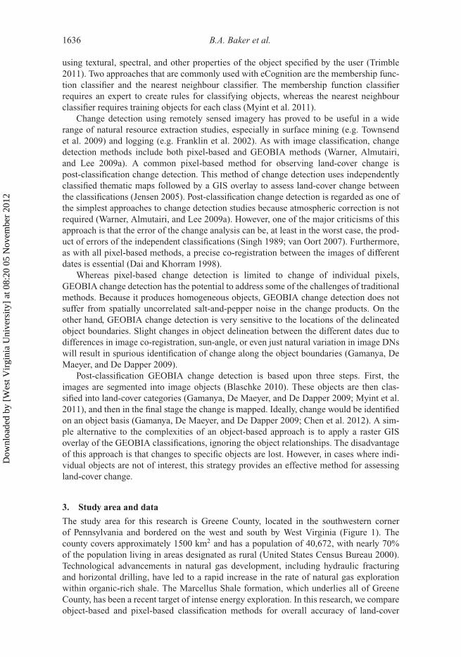
Figure 3. Research flow chart showing the main steps in methods and analysis.

for normalization (Figure 3). Although the majority of the tiles appear to be matched wellwith this procedure, it was not possible to remove minor differences between a few tiles dueto differences in shadowing, vegetation phenology, and other image artefacts. Next, the 1 mimagery was resampled to coarser spatial resolutions through averaging of adjacent pixelsto produce four additional images at 2, 5, 15, and 30 m (Figure 3). The upper limit of 30 mwas chosen to coincide with the Landsat pixel size, and also to ensure that the pixel size wasalways smaller than that of the smallest well pad. The resampling approach was selected inorder to ensure the maximum spectral and phenological consistency between the images ofthe various scales, which would be hard to achieve if images from different sensors wereused (Yang and Merchant 1997). These preprocessing steps were performed using both the2004 and 2010 imagery, to produce a total of 10 images (two dates, five scales) used in theclassification and analysis.

A qualitative visual comparison through overlaying the 2004 and 2010 images sug-gested that although the co-registration error is mostly less than 1 m (i.e. 1 pixel), in placesthe error is as high as 3 m, most likely due to limitations of the data used in the orthorecti-fication of the original photographs, such as the digital elevation model. The distribution oferror appeared to be random, and attempts to reduce the error through warping one imageto match the other were not successful. Further geometric co-registration was therefore notperformed. Because the size of the gas well clearings is much greater than this error (seenext section), and the vast majority of the images were co-registered with an error of lessthan 1 pixel, co-registration error was not regarded as likely to have a major impact on theresults.

4.2. Land-cover classifications

A binary classification scheme using only Forest and Non-forest classes was used to classifythe 2004 and 2010 images at each spatial resolution using the three spectral bands commonto both data sets (green, red, and near-infrared bands). Forest was defined as patches oftree cover exceeding a minimum mapping unit (MMU) of 1800 m2 (equivalent to the area

Dow

nloa

ded

by [

Wes

t Vir

gini

a U

nive

rsity

] at

08:

20 0

5 N

ovem

ber

2012

International Journal of Remote Sensing 1639

of 1800 1 m pixels, or two 30 m pixels). Non-forest was defined as all other land-coverclasses. These class definitions were used for both the 2004 and 2010 images at each of thefive spatial resolutions.

Maximum likelihood classification was used for the pixel-based classification to pro-duce thematic maps of land cover for both image dates. Maximum likelihood classificationwas chosen to benchmark the pixel-based methods because it is regarded as a standardapproach, and is highly effective if the classes at least approximately satisfy the assumptionof multivariate normality (Swain and Davis 1978; Jensen et al. 2009). To ensure that theclassification results were optimal, a hierarchical approach was adopted. The two classes ofinterest, Forest and Non-forest, were each subdivided into multiple spectral subclasses,representing all distinct classes in the scene including buildings, paved surfaces, opengrasslands, bare soil, agricultural fields, and water. For example, within the paved class,a spectral subclass of bright impervious surfaces was identified. Five to ten separate sets oftraining samples were then collected for each spectrally distinct subclass. These individualtraining samples were treated as separate spectral classes, which were merged only afterclassification. A thematic map was produced for each spatial resolution of the 2004 and2010 images and then overlaid to produce a final map of land-cover change at each ofthe resolutions. These images were filtered using the Erdas Imagine 2011 ‘Clump’ and‘Eliminate’ processes to remove patches less than the MMU of 1800 m2 for all types ofland-cover classes and to replace the land-cover value with the same class as the majorityof the surrounding pixels (Newman, Mclaren, and Wilson 2011).

Object-based classifications were performed using eCognition Developer 8 (Trimble2011). The multiresolution segmentation algorithm was used to segment each of theimages, with a trial-and-error approach used to determine the optimal scale, shape, andcompactness segmentation parameters. The final parameters chosen were 0.1 for shape,0.5 for compactness, and scale parameters that varied as a function of pixel size: 25 for1 and 2 m pixels, 10 for 5 m pixels, and 5 for 15 and 30 m pixels. All three spectral bandswere used in the segmentation, with the near-infrared band weighted twice as much as thegreen and red bands because the forest class is most distinctive at these wavelengths.

Once the image segmentations were produced, rulesets were developed by testing arange of rules for classifying Forest and Non-forest objects using a trial-and-error approach.The rules included thresholds for mean brightness, standard deviation of single bands, meanvalues of single bands, and a normalized difference vegetation index (NDVI) ratio param-eter (Tucker 1979). The same rules were used for each classification, although thresholdsof the parameters were manually adjusted to produce what was qualitatively determined tobe the optimal classification for each of the five scales for each of the two dates. Rasterizedpolygon classifications were exported from eCognition Developer 8 and overlaid to pro-duce the map of change objects. The maps of land-cover change were then filtered usingthe same logical filtering methods as the pixel-based classifications to eliminate objectssmaller than the MMU.

4.3. Land-cover change map accuracy assessment

Accuracy assessments were performed for the maps of land-cover change using a visualinterpretation of the 1 m images as the reference data source. The number of sample pointswas determined using a multinomial distribution based on the number of classes (fourchange classes), the proportion of the largest class (approximately 60% forest), and a 95%confidence level with 7% precision (Congalton and Green 2009). The estimated necessarysample size was rounded up, and 300 randomly generated points were used for accuracy

Dow

nloa

ded

by [

Wes

t Vir

gini

a U

nive

rsity

] at

08:

20 0

5 N

ovem

ber

2012

1640 B.A. Baker et al.

assessment of the thematic maps produced using the pixel-based maximum likelihood clas-sification method. The same points were used for each of the land-cover change maps atthe five resolutions.

Although the kappa statistic (Cohen 1960) is a common summary accuracy measure,its use in remote sensing has been increasingly questioned (e.g. Stehman and Foody 2009).Pontius and Millones (2011) propose quantity and allocation disagreement as alternativemeasures. Quantity disagreement is defined as the difference between the reference dataand the classified data based upon mismatch of class proportions. Allocation disagreementcan be considered as the difference between the classified data and the reference data dueto incorrect spatial allocations of pixels in the classification. The total disagreement is thesum of the quantity and allocation disagreements (Pontius and Millones 2011).

A review of the literature by Rakshit (2012) reveals that there is no standardizedmethod for accuracy assessment of object-based classifications. However, Congalton andGreen (2009) have suggested that objects should be the sampling units of thematic accu-racy assessment for maps produced using GEOBIA methods. In this research, the unitfor the object-oriented accuracy polygons of assessment was the change polygon, definedby the intersection of the two underlying dates (Figure 4). The object-based method ofaccuracy assessment consisted of two parts. First, the points employed in the pixel-basedaccuracy assessment were used in eCognition Developer 8 to extract the objects from boththe 2004 and 2010 classifications, which contained the randomly selected sample points.These separate sets of objects were then intersected using ArcMap 10 (ESRI, Redlands,California) and the intersection of the two objects was used as the polygons for accuracyassessment. The majority cover type of this polygon was used as the reference class, asrecommended by Dorren, Maier, and Seijmonsbergen (2003). Overall accuracy of object-based maps was calculated on an area-weighted basis, in which the summed area ofcorrectly classified objects is divided by the total area of all objects used in the assessment.

A comparison of thematic map accuracies of the final change products was performedto investigate how overall accuracy changed with spatial resolution, as well as how accuracyvaried between classification methods. Uncertainty estimates were also calculated using amodified version of the equation used to determine the sample size based on binomialprobability theory (Jensen 2005):

E =√

Z2pq

N, (1)

where E is the error estimate for a specified sample size, N , with accuracy p and con-fidence level q = 100 – p (Fitzpatrick-Lins 1981). The value for Z is 2 in this equationand is an approximation of the standard normal deviate of 1.96 for the 95% two-sidedconfidence level. Error estimates were calculated to determine statistical differentiation ofoverall thematic accuracy from another.

4.4. Land-cover change of new clearings accuracy assessment

In addition to investigating how overall accuracy varies with spatial scale and classificationmethod, we also examined how scale and classification method affect accuracy for identifi-cation of new clearings within forested areas associated with natural gas development. Thegas well point data set was used to identify the wells that were not present in 2004 and werepresent in the 2010 imagery (i.e. the land cover went from Forest to Non-forest). Assessingland-cover change using the point data set of well locations is not straightforward, since

Dow

nloa

ded

by [

Wes

t Vir

gini

a U

nive

rsity

] at

08:

20 0

5 N

ovem

ber

2012

International Journal of Remote Sensing 1641

2010 object

2004 object

Accuracy assessment point

Intersected object

Figure 4. Example of object-based accuracy assessment polygon.

the features of interest, well clearings, comprise areas, not points. Therefore, 180 new wellpermit point locations were randomly selected throughout the county and the extent of eachwell pad clearing was manually digitized using the 1 m imagery. This manually digitizedpolygon included only the well clearing, and excluded access roads to the sites that weresometimes visible. All polygons included in the accuracy assessment were greater than theMMU of 1800 m2.

The well clearing polygons were then converted to raster files, one for each of the fivespatial resolutions studied, and the land-cover classes mapped in the change analysis withineach clearing were summarized using the land-cover change maps of both classification

Dow

nloa

ded

by [

Wes

t Vir

gini

a U

nive

rsity

] at

08:

20 0

5 N

ovem

ber

2012

1642 B.A. Baker et al.

methods for each of the respective spatial resolutions. The total area of each class from thesample of 180 clearings was tabulated and the proportion of correctly identified land-coverchange within each polygon was summarized. Each polygon well clearing was assumed torepresent the ‘Forest to non-forest’ change class and a percentage of correctly identifiedchange was calculated to provide a measure of how well each classification method andspatial resolution combination identified land-cover change of well clearings.

5. Results and discussion

5.1. Land-cover classification comparison

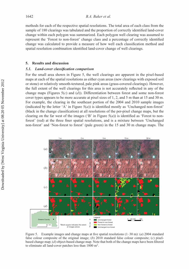
For the small area shown in Figure 5, the well clearings are apparent in the pixel-basedmaps at each of the spatial resolutions as either cyan areas (new clearings with exposed soilor stone) or relatively smooth-textured, pale pink areas (grass-covered clearings). However,the full extent of the well clearings for this area is not accurately reflected in any of thechange maps (Figures 5(c) and (d)). Differentiation between forest and some non-forestcover types appears to be more accurate at pixel sizes of 1, 2, and 5 m than at 15 and 30 m.For example, the clearing in the southeast portion of the 2004 and 2010 sample images(indicated by the letter ‘A’ in Figure 5(a)) is identified mostly as ‘Unchanged non-forest’(black in the change classification) at all resolutions of the per-pixel change maps, but theclearing on the far west of the images (‘B’ in Figure 5(a)) is identified as ‘Forest to non-forest’ (red) at the three finer spatial resolutions, and is a mixture between ‘Unchangednon-forest’ and ‘Non-forest to forest’ (pale green) in the 15 and 30 m change maps. The

1 m

*Black square indicates the extentof images above

km200

m500125 2500Greene County

30 m15 m5 m2 m

NLegend

Unchanged forest

Unchanged non-forestNon-forest to forestForest to non-forest

(a)

(b)

(d)

(c)

Figure 5. Example images and change maps at five spatial resolutions (1–30 m): (a) 2004 standardfalse colour composite of the original image; (b) 2010 standard false colour composite; (c) pixel-based change map; (d) object-based change map. Note that both of the change maps have been filteredto eliminate all land-cover patches less than 1800 m2.

Dow

nloa

ded

by [

Wes

t Vir

gini

a U

nive

rsity

] at

08:

20 0

5 N

ovem

ber

2012

International Journal of Remote Sensing 1643

‘Non-forest to forest class’ is primarily in areas that were in fact forest in both images anddid not change over the time period. This indicates that the areas were misclassified in the2004 image but were correctly classified in the 2010 image. Visual inspection of the mapsof land-cover change produced using the pixel-based maximum likelihood classificationmethod indicates a slight variation in the classifications as the spatial resolution changes,although the well clearings are identified reasonably well at all spatial resolutions.

The GEOBIA-based classification identified the disturbed forest associated with eachwell clearing, although the extent of the clearings is not as evident for some clearings asit was in the pixel-based classifications (Figure 5(d)). For example, the well clearing inthe northwest portion of the sample figures (‘C’ in Figure 5(b)) shows a new clearing in2010, but the 2, 5, and 15 m object-based maps of land-cover change indicate ‘Unchangedforest’ as the land-cover class for portions of this clearing. Although less common than inthe pixel-based classification maps, the presence of the ‘Non-forest to forest’ class in allfive classifications is an error within the classifications of this particular area, as withinthe region shown, there were no areas identified as new forest growth within the 6 yearsbetween images. As one might expect, minor land-cover changes such as access roads towells are better identified at finer resolutions between 1 and 5 m, although none of the mapsfully and accurately identify the entire extent of these smaller changes to the forest, mostlikely due to the smoothing applied to the pixel-based classifications, and the aggregationinherent in GEOBIA classifications. Varying illumination and view angle effects in theaerial imagery may also have played a role in limiting the ability to identify small changes,as well as co-registration differences at the 1 m scale.

The most common classification errors for both methods came from similaritiesbetween DN values of forest pixels or objects and other vegetated pixels or objects. This ledto the misclassification of some agricultural fields as forest, because brightly illuminatedforest had similar reflectance to other vegetation. Classification error of this type explainssome of the land-cover change classified as ‘Non-forest to forest’.

5.2. Land-cover change map accuracy assessment comparison

The 1 m object-based classification was the most accurate of all the classificationmethod/spatial resolution combinations. The most accurate pixel-based map of land-coverchange produced (Table 1) was the 5 m map at 81.6%, although the 1 and 2 m maps had only

Table 1. Summary of overall accuracy, quantity disagreement, and allocation disagreement forpixel- and object-based maps of land-cover change as a function of pixel size.

Classificationmethod Pixel size (m)

Overallaccuracy (%)

Quantitydisagreement

Allocationdisagreement

Pixel-based 1 81.3 0.11 0.072 81.3 0.12 0.075 81.6 0.12 0.06

15 76.0 0.17 0.0730 75.6 0.12 0.12

Object-based 1 87.1 0.07 0.072 80.1 0.14 0.065 82.3 0.12 0.06

15 74.7 0.21 0.0630 76.0 0.12 0.13

Dow

nloa

ded

by [

Wes

t Vir

gini

a U

nive

rsity

] at

08:

20 0

5 N

ovem

ber

2012

1644 B.A. Baker et al.

100

95

90

Ove

rall

accu

racy

(%

)

85

80

75

70

Object-based

Pixel-based65

600 5 10 15

Spatial resolution (m)20 25 30

Figure 6. Comparison of overall accuracy of land-cover change maps for pixel-based and object-based classification methods of five spatial resolutions. Error bars indicate 95% confidence interval.

slightly lower accuracy. The 15 and 30 m resolution map accuracies were notably lower, at76.0% and 75.6%, respectively. For the object-based series of maps, the most accurate clas-sification was the 1 m map at 87.1%, and the 5 m map at 82.3% was the second mostaccurate classification. As with the pixel-based classification, the 15 and 30 m object-basedchange maps had notably lower accuracies than the finer resolution classifications.

Figure 6, showing the uncertainty associated with these accuracies, indicates that the1 m object-based classification was statistically more accurate than the 15 and 30 m mapsof both pixel- and object-based methods. This result suggests that fine spatial resolu-tion does seem to favour GEOBIA. Despite this finding, the classifications at scales of2–30 m were not statistically different, suggesting that if cost and availability limit accessto the very finest scales, moderate resolution data, analysed using pixel-based classifica-tion methods, can suffice in place of 2–5 m data and the more complex, object-basedclassification. However, for any single spatial resolution, the accuracy of the object-basedchange map is not statistically different from that of the pixel-based change map at the sameresolution. This general lack of statistical difference between object- and pixel-based meth-ods applied at the same scale suggests that pixel-based classification combined with thepost-classification filtering process, which eliminated some of the salt-and-pepper effectcommon to pixel-based classifications, may be as effective as GEOBIA change analysis,especially at scales coarser than 1 m.

The quantity disagreement values, which give information on the error in the rela-tive proportion of the classes in the map, range from 0.07 to 0.21 for both pixel- andobject-based classification methods (Table 1). The quantity disagreement values were moreconsistent across scales for the pixel-based classification than the object-based classifi-cation, which had both the lowest and the highest values observed. For both the pixel-and object-based classifications, the highest quantity disagreement values were found for

Dow

nloa

ded

by [

Wes

t Vir

gini

a U

nive

rsity

] at

08:

20 0

5 N

ovem

ber

2012

International Journal of Remote Sensing 1645

maps produced with 15 m pixels. Allocation disagreement was very similar (0.06–0.07) forthe object-based and pixel-based maps for pixels of 2–30 m, but was noticeably higherat the 30 m pixel scale (0.12–0.13). This suggests that at coarser spatial resolutions, wellsite spectral properties become less separable for pixel-based classifications. In combina-tion, the two measures of accuracy imply that the proportion of pixels assigned to eachclass was a source of error more often than the spatial allocation of classes within theclassifications.

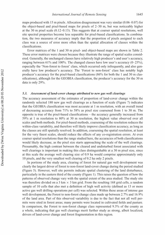
Error matrices of the 1 and 30 m pixel- and object-based maps are shown in Table 2.These error matrices were chosen because they illustrate the range of spatial scales consid-ered. Generally, the unchanged classes have relatively high producer’s and user’s accuracy,ranging between 61% and 100%. The changed classes have low user’s accuracy (0–25%),especially the ‘Non-forest to forest’ class, which occurred only infrequently, and also gen-erally have low producer’s accuracy. The ‘Forest to non-forest’ class has notably highproducer’s accuracy for the pixel-based classifications (86% for both the 1 and 30 m clas-sifications), although for the GEOBIA classification, the producer’s accuracy for the 30 mdata is only 29%.

5.3. Assessment of land-cover change attributed to new gas well clearings

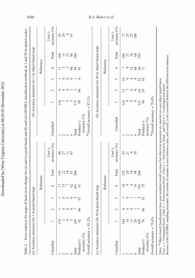
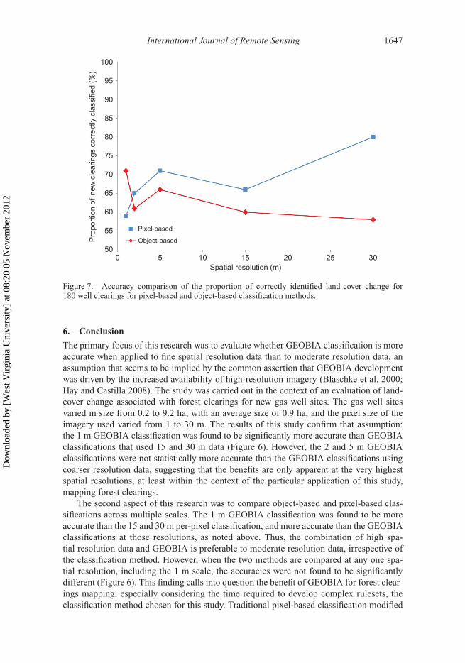
The accuracy assessment of the estimates of proportion of land-cover change within therandomly selected 180 new gas well clearings as a function of scale (Figure 7) indicatesthat the GEOBIA classification was most accurate at 1 m resolution, with an overall trendof decreasing accuracy from 71% to 58% as pixel size coarsened from 1 to 30 m. Theopposite is true of the pixel-based classifications – the accuracy generally increased from59% at 1 m resolution to 80% at 30 m resolution, the highest value observed over allscales and both methods. For pixel-based methods, coarsening of the resolution reduces thewithin-class variability, and therefore will likely improve classification accuracy, as long asthe classes are still spatially resolved. In addition, coarsening the spatial resolution, at leastfor the very finest scales, should reduce the effects of any co-registration errors. At evencoarser spatial resolutions than the range studied here, the accuracies of both classificationswould likely decrease, as the pixel size starts approaching the scale of the well clearings.Presumably, the high contrast between the cleared and undisturbed forest associated withwell clearings is important in making this class distinguishable at a 30 m pixel size, sinceat this scale the average well clearing size of 0.9 ha would comprise approximately only10 pixels, and the very smallest well clearing of 0.2 ha only 2 pixels.

In portions of the study area, clearing of forest for natural gas well development wasclearly the largest driver of forest to non-forest land-cover change during the period studied(Figure 5). However, well site permits indicate spatial clustering of the land disturbance,particularly in the eastern third of the county (Figure 1). This raises the question of how thepatterns of observed change vary with the spatial extent of the area studied. The study sitewas therefore divided on a 3 km × 3 km grid. From the resulting 168 grid cells, a randomsample of 10 cells that also met a definition of high well activity (defined as 13 or moreactive gas well drilling operations per cell) was selected. Within these areas of intense gaswell development, the Forest to non-forest change class made up between 2.7% and 16.9%of the land area. Part of this observed variability is due to the fact that not all well per-mits were sited in forest areas; many permits were located in cultivated fields and pasture.In comparison, the Forest to non-forest change class represented 9.3% of the county asa whole, indicating that gas well clearings merit further study as strong, albeit localized,drivers of land-cover change and forest fragmentation in this region.

Dow

nloa

ded

by [

Wes

t Vir

gini

a U

nive

rsity

] at

08:

20 0

5 N

ovem

ber

2012

1646 B.A. Baker et al.

Tabl

e2.

Err

orm

atri

ces

for

map

sof

land

-cov

erch

ange

for

(a)

and

(c)

pixe

l-ba

sed

and

(b)

and

(d)

GE

OB

IAcl

assi

fica

tion

met

hods

at1

and

30m

spat

ials

cale

s.

(a)

Acc

urac

ym

easu

res

for

1m

pixe

l-ba

sed

map

(b)

Acc

urac

ym

easu

res

for

1m

obje

ct-b

ased

map

Ref

eren

ceR

efer

ence

Cla

ssifi

ed1

23

4To

tal

Use

r’s

accu

racy

(%)

Cla

ssifi

ed1

23

4To

tal

Use

r’s

accu

racy

(%)

117

41

117

193

901

156

01

1116

893

21

60

1522

272

54

05

1429

39

02

718

113

90

03

120

45

00

6267

934

51

080

8693

Tota

l18

97

310

130

0To

tal

175

51

9928

0P

rodu

cer’

sac

cura

cy(%

)92

8667

61P

rodu

cer’

sac

cura

cy(%

)89

800

81

Ove

rall

accu

racy

=81

.3%

*O

vera

llac

cura

cy=

87.1

%

(c)

Acc

urac

ym

easu

res

for

30m

pixe

l-ba

sed

map

(d)

Acc

urac

ym

easu

res

for

30m

obje

ct-b

ased

map

Ref

eren

ceR

efer

ence

Cla

ssifi

ed1

23

4To

tal

Use

r’s

accu

racy

(%)

Cla

ssifi

ed1

23

4To

tal

Use

r’s

accu

racy

(%)

114

40

110

155

931

142

1718

718

477

214

60

929

212

97

09

2528

311

01

618

63

00

412

1625

420

11

7698

784

00

068

6810

0To

tal

189

73

101

300

Tota

l15

124

2296

293

Pro

duce

r’s

accu

racy

(%)

7686

3375

Pro

duce

r’s

accu

racy

(%)

9429

1871

Ove

rall

accu

racy

=75

.6%

*O

vera

llac

cura

cy=

76.0

%

Not

es:*

Obj

ect-

base

dcl

assi

fica

tion

sha

vear

ea-w

eigh

ted

over

alla

ccur

acy

buto

ther

wis

eac

cura

cies

are

repo

rted

ona

per-

obje

ct(p

ixel

)ba

sis.

Cla

ss1

=‘U

ncha

nged

fore

st’,

Cla

ss2

=‘F

ores

tto

non-

fore

st’,

Cla

ss3

=‘N

on-f

ores

tto

fore

st’,

and

Cla

ss4

=‘U

ncha

nged

non-

fore

st’.

Bec

ause

ofth

eG

EO

BIA

sam

plin

gpr

oced

ure,

the

num

ber

ofsa

mpl

esin

each

refe

renc

ecl

ass,

and

over

all,

isno

tcon

sist

entb

etw

een

the

diff

eren

terr

orm

atri

ces.

Dow

nloa

ded

by [

Wes

t Vir

gini

a U

nive

rsity

] at

08:

20 0

5 N

ovem

ber

2012

International Journal of Remote Sensing 1647

100

95

90

85

80

75

70

65

60

55

500 5 10 15 20 25 30

Object-based

Pixel-based

Spatial resolution (m)

Pro

port

ion

of n

ew c

lear

ings

cor

rect

ly c

lass

ified

(%

)

Figure 7. Accuracy comparison of the proportion of correctly identified land-cover change for180 well clearings for pixel-based and object-based classification methods.

6. Conclusion

The primary focus of this research was to evaluate whether GEOBIA classification is moreaccurate when applied to fine spatial resolution data than to moderate resolution data, anassumption that seems to be implied by the common assertion that GEOBIA developmentwas driven by the increased availability of high-resolution imagery (Blaschke et al. 2000;Hay and Castilla 2008). The study was carried out in the context of an evaluation of land-cover change associated with forest clearings for new gas well sites. The gas well sitesvaried in size from 0.2 to 9.2 ha, with an average size of 0.9 ha, and the pixel size of theimagery used varied from 1 to 30 m. The results of this study confirm that assumption:the 1 m GEOBIA classification was found to be significantly more accurate than GEOBIAclassifications that used 15 and 30 m data (Figure 6). However, the 2 and 5 m GEOBIAclassifications were not statistically more accurate than the GEOBIA classifications usingcoarser resolution data, suggesting that the benefits are only apparent at the very highestspatial resolutions, at least within the context of the particular application of this study,mapping forest clearings.

The second aspect of this research was to compare object-based and pixel-based clas-sifications across multiple scales. The 1 m GEOBIA classification was found to be moreaccurate than the 15 and 30 m per-pixel classification, and more accurate than the GEOBIAclassifications at those resolutions, as noted above. Thus, the combination of high spa-tial resolution data and GEOBIA is preferable to moderate resolution data, irrespective ofthe classification method. However, when the two methods are compared at any one spa-tial resolution, including the 1 m scale, the accuracies were not found to be significantlydifferent (Figure 6). This finding calls into question the benefit of GEOBIA for forest clear-ings mapping, especially considering the time required to develop complex rulesets, theclassification method chosen for this study. Traditional pixel-based classification modified

Dow

nloa

ded

by [

Wes

t Vir

gini

a U

nive

rsity

] at

08:

20 0

5 N

ovem

ber

2012

1648 B.A. Baker et al.

using a simple post-classification smoothing technique appears to be a viable alternative toGEOBIA.

When the proportion of new well clearings correctly mapped was investigated(Figure 7), pixel-based classification generally increased in accuracy, and the GEOBIAclassification accuracy declined, as the pixel size used changed from 1 to 30 m. Only at the1 m scale was the GEOBIA classification more accurate than the pixel-based classification.

This research has implications for future studies focused on object-based and pixel-based classifications. Spatial resolution is only one of the characteristics of imagery thataffect thematic map accuracy (Warner, Nellis, and Foody 2009b), and generalizing fromthese results will require consideration of the underlying mapping problem of interest.Object-based methods are potentially more effective than pixel-based methods if the classeshave high internal variability, and the classes of interest cover large areas relative to thepixel size. Per-pixel methods are more likely to be successful where the classes of interestoccur in patches that are at time relatively small.

One of the challenges of this work was to define a consistent and logical GEOBIAchange detection accuracy evaluation procedure. The approach developed for this studyserved the needs of the project well, but further work in developing optimal accuracyevaluation methods should be a high priority.

Practical limitations would also be important if this procedure were to be conductedin an operational setting. The original 1 m imagery of the entire county required approxi-mately 10 GB of disk space and took more than 4 h to segment and classify on a 3.2 GHzQuad Core i7 computer, with 24 GB of RAM. The large images also caused softwarecrashes, and the large number of polygons generated in the GEOBIA analysis at 1 mappeared to exceed the file format limits. In practice, therefore, fine spatial resolution datamay not be appropriate for large regional mapping applications. These problems reinforcethe concern that high spatial resolution comes with trade-offs (Warner, Nellis, and Foody2009b; Warner 2010).

The data used in this project consisted of US government NAIP imagery, which isincreasingly used in research projects (e.g. Crimmins, Mynsberge, and Warner 2009)because of its minimal cost and relatively frequent repeat acquisition. However, the useof NAIP aerial imagery for evaluating land-cover change poses several distinctive chal-lenges compared to other data sources. Mosaicking quarter quadrangle tiles collected overan entire growing season leads to differences in DN values across multiple image tilesas plant phenology, time of day, and illumination vary between image acquisition times.Histogram matching of overlap areas helped normalize some of these differences but someimage tiles were still noticeably different. Also, although shadows tend to be consistent atleast within individual quarter quadrangle tiles, they are challenging to classify correctly,especially within-forest shadows that may be misclassified as forest clearings.

The ideal for a project of the nature studied here would be to use satellite data that coverthe entire study area in one image. This would reduce within-scene variations in phenologyand illumination, at least for study areas of size similar to that in this study, and withoutnotable climate gradients. However, scale does remain an important issue. Although 30 mimagery (such as Landsat) could potentially be used to monitor this type of land-coverchange, it is unlikely that imagery coarser than 30 m spatial resolution would prove usefulfor observing this process, because the clearings average only 0.9 ha in size. The temporalresolution of the sensor also factors into the ability to accurately classify and assess land-cover change, because gas well clearings could potentially be cleared and re-vegetated withgrass or shrubs in a relatively short period of time, making clearings more spectrally similarto the surrounding forest. Therefore, a satellite-borne data source with a spatial resolution

Dow

nloa

ded

by [

Wes

t Vir

gini

a U

nive

rsity

] at

08:

20 0

5 N

ovem

ber

2012

International Journal of Remote Sensing 1649

finer than 30 m (such as the Advanced Spaceborne Thermal Emission and ReflectanceRadiometer (ASTER)) and with the ability to acquire images at yearly intervals would bemost effective for monitoring land-cover change associated with natural gas development.

AcknowledgementsThe authors thank the two anonymous reviewers for their important insights, which improved thisarticle. West Virginia View provided support for this research.

ReferencesBaatz, M., and A. Schäpe. 2000. “Multiresolution Segmentation – An Optimization Approach

for High Quality Multi-Scale Image Segmentation.” In Angewandte GeographischeInformationsverarbeitung XII , edited by J. Strobl, T. Blaschke, and G. Griesebener, 12–23.Berlin: Herbert Wichmann Verlag.

Blaschke, T. 2010. “Object Based Image Analysis for Remote Sensing.” ISPRS Journal ofPhotogrammetry and Remote Sensing 65: 2–16.

Blaschke, T., S. Lang, E. Lorup, J. Strobl, and P. Zeil. 2000. “Object-Oriented Image Processing in anIntegrated GIS/Remote Sensing Environment and Perspectives for Environmental Applications.”In Environmental Information for Planning, Politics, and the Public, Vol. 2, edited by A. Cremersand K. Greve, 555–70. Marburg: Metropolis Verlag.

Chen, G., G. J. Hay, L. M. T. Carvalho, and M. A. Wulder. 2012. “Object-Based Change Detection.”International Journal of Remote Sensing 33: 4434–57.

Cohen, J. 1960. “A Coefficient of Agreement for Nominal Scales.” Educational and PsychologicalMeasurement 20: 37–46.

Congalton, R. G., and Green, K., eds. 2009. Assessing the Accuracy of Remotely Sensed Data:Principles and Practices. 2nd ed., 182 pp. Boca Raton, FL: CRC Press.

Crimmins, S., A. Mynsberge, and T. A. Warner. 2009. “Estimating Woody BrowseAbundance from Aerial Imagery.” International Journal of Remote Sensing 30: 3283–9.doi:10.1080/01431160902777167.

Dai, X., and S. Khorram. 1998. “The Effect of Image Misregistration on the Accuracy of RemotelySensed Change Detection.” IEEE Transactions on Geoscience and Remote Sensing 36: 1566–77.

Dorren, L. K. A., B. Maier, and A. C. Seijmonsbergen. 2003. “Improved Landsat-Based ForestMapping in Steep Mountainous Terrain Using Object-Based Classification.” Forest Ecology andManagement 183: 31–46.

Dragut, L., and C. Eisank. 2011. “Object Representations at Multiple Scales from Digital ElevationModels.” Geomorphology 129: 183–9.

ERDAS. 2011. Erdas Imagine 2011 User Manual. Norcross, GA: ERDAS Inc.Fenneman, N. M. 1917. “Physiographic Subdivisions of the United States.” Proceedings of the

National Academy of Sciences of the United States of America 3: 17–22.Fitzpatrick-Lins, K. 1981. “Comparison of Sampling Procedures and Data Analysis for a Land-Use

and Land-Cover Map.” Photogrammetric Engineering & Remote Sensing 47: 343–51.Franklin, S. E., M. B. Lavigne, M. A. Wulder, and G. B. Stenhouse. 2002. “Change Detection and

Landscape Structure Mapping Using Remote Sensing.” The Forestry Chronicle 78: 618–25.Gamanya, R., P. De Maeyer, and M. De Dapper. 2009. “Object-Oriented Change Detection for the

City of Harare, Zimbabwe.” Expert Systems with Applications 36: 571–88.Giner, N., and J. Rogan. 2012. “A Comparison of Landsat ETM+ and High-Resolution Aerial

Orthophotos to Map Urban/Suburban Forest Cover in Massachusetts, USA.” Remote SensingLetters 3: 667–76.

Hay, G. J., and G. Castilla. 2008. “Geographic Object-Based Image Analysis (GEOBIA): A NewName for a New Discipline.” In Object-Based Image Analysis, edited by T. Blaschke, S. Lang,and G. J. Hay. Berlin: Springer.

Jensen, J. R. 2005. Introductory Digital Image Processing: A Remote Sensing Perspective. 3rd ed.,526 pp. Upper Saddle River, NJ: Prentice-Hall.

Jensen, J. R., J. Im, P. Hardin, and R. R. Jensen. 2009. “Image Classification.” In SAGE Handbook ofRemote Sensing, edited by T. A. Warner, M. D. Nellis, and G. M. Foody, 267–81. London: Sage.

Dow

nloa

ded

by [

Wes

t Vir

gini

a U

nive

rsity

] at

08:

20 0

5 N

ovem

ber

2012

1650 B.A. Baker et al.

Johansen, K., L. A. Arroyo, S. Phinn, and C. Witte. 2010. “Comparison of Geo-Object Basedand Pixel-Based Change Detection of Riparian Environments Using High Spatial ResolutionMultispectral Imagery.” Photogrammetric Engineering & Remote Sensing 76: 123–36.

Kim, M., M. Madden, and T. A. Warner. 2009. “Forest Type Mapping Using Object-Specific TextureMeasures from Multispectral IKONOS Imagery: Segmentation Quality and Image ClassificationIssues.” Photogrammetric Engineering and Remote Sensing 75: 819–29.

Kim, M., T. A. Warner, M. Madden, and D. Atkinson. 2011. “Multi-Scale Texture Segmentation andClassification of Salt Marsh Using Digital Aerial Imagery with Very High Spatial Resolution.”International Journal of Remote Sensing 32: 2825–50. doi:10.1080/01431161003745608.

Liu, D., and F. Xia. 2010. “Assessing Object-Based Classification: Advantages and Limitations.”Remote Sensing Letters 1: 187–94. doi:10.1080/01431161003743173.

Malinverni, E. S., A. N. Tassetti, A. Mancini, P. Zingaretti, E. Frontoni, and A. Bernardini.2011. “Hybrid Object-Based Approach for Land Use/Land Cover Mapping Using High SpatialResolution Imagery.” International Journal of Geographic Information Science 25: 1025–43.

Matinfar, H. R., F. Sarmadian, S. K. Alavi Panah, and R. J. Heck. 2007. “Comparisons of Object-Oriented and Pixel-Based Classification of Land Use/Land Cover Types Based on LandsatETM+ Spectral Bands (Case Study: Arid Region of Iran).” American-Eurasian Journal ofAgriculture and Environmental Science 2: 448–56.

Myint, S. W., P. Gober, A. Brazel, S. Grossman-Clarke, and Q. Weng. 2011. “Per-Pixel vs. Object-Based Classification of Urban Land Cover Extraction Using High Spatial Resolution Imagery.”Remote Sensing of Environment 115: 1145–61.

Newman, M. E., K. P. Mclaren, and B. S. Wilson. 2011. “Comparing the Effects of ClassificationTechniques on Landscape-Level Assessments: Pixel-Based Versus Object-Based Classification.”International Journal of Remote Sensing 32: 4055–73.

Platt, R. V., and A. F. H. Goetz. 2004. “A Comparison of AVIRIS and Synthetic Landsat Data forLand Use Classification at the Urban Fringe.” Photogrammetric Engineering & Remote Sensing70: 813–19.

Platt, R. V., and L. Rapoza. 2008. “An Evaluation of an Object-Oriented Paradigm for Land Use/LandCover Classification.” The Professional Geographer 60: 87–100.

Pontius Jr, R. G., and M. Millones. 2011. “Death to Kappa: Birth of Quantity Disagreement andAllocation Disagreement for Accuracy Assessment.” International Journal of Remote Sensing32: 4407–29.

Pringle, R. M., M. Syfert, J. K. Webb, and R. Shine. 2009. “Quantifying Historical Changes in HabitatAvailability for Endangered Species: Use of Pixel- and Object-Based Remote Sensing.” Journalof Applied Ecology 46: 544–53.

Rakshit, R. 2012. “A Survey of Accuracy Measures in Object-Based Image Analysis Maps.” PhDthesis, Clark University.

Robertson, L. D., and D. J. King. 2011. “Comparison of Pixel- and Object-Based Classification inLand Cover Change Mapping.” International Journal of Remote Sensing 32: 1505–29.

Singh, A. 1989. “Digital Change Detection Techniques Using Remotely-Sensed Data.” InternationalJournal of Remote Sensing 10: 989–1003.

Stehman, S. V., and G. M. Foody. 2009. “Accuracy Assessment.” In The SAGE Handbook of RemoteSensing, edited by T. A. Warner, M. D. Nellis, and G. M. Foody, 297–309. Thousand Oaks, CA:Sage Publications.

Swain, P. H., and S. M. Davis. 1978. Remote Sensing: The Quantitative Approach. New York:McGraw-Hill.

Townsend, F. 1986. “The Enhancement of Computer Classifications by Logical Smoothing.”Photogrammetric Engineering & Remote Sensing 52: 213–21.

Townsend, P. A., D. P. Helmers, C. C. Kingdon, B. E. Mcneil, K. M. De Beurs, and K. N. Eshleman.2009. “Changes in the Extent of Surface Mining and Reclamation in the Central AppalachiansDetected Using a 1976–2006 Landsat Time Series.” Remote Sensing of Environment 113: 62–72.

Trimble. 2011. ECognition Developer 8.64.1 User Guide. Munich: Trimble Germany.Tucker, C. J. 1979. “Red and Photographic Infrared Linear Combinations for Monitoring Vegetation.”

Remote Sensing of Environment 8: 127–50.United States Census Bureau. 2000. Census 2000 Decennial Census Data (accessed May 12, 2011).

http://factfinder.census.gov/home/saff/main.html?_lang=en.Van Oort, P. A. J. 2007. “Interpreting the Change Detection Error Matrix.” Remote Sensing of

Environment 108: 1–8. doi:10.1016/j.rse.2006.10.012.

Dow

nloa

ded

by [

Wes

t Vir

gini

a U

nive

rsity

] at

08:

20 0

5 N

ovem

ber

2012

International Journal of Remote Sensing 1651

Warner, T. A. 2010. “Remote Sensing Analysis: From Project Design to Implementation.” Chap. 17in Manual of Geospatial Sciences, 2nd ed., edited by J. D. Bossler, R. B. McMaster, C. Rizos,and J. B. Campbell, 301–18. London: Taylor and Francis.

Warner, T. A., A. Almutairi, and J. Y. Lee. 2009a. “Remote Sensing of Land Cover Change.” In TheSAGE Handbook of Remote Sensing, edited by T. A. Warner, M. D. Nellis, and G. M. Foody,459–72. Thousand Oaks, CA: Sage Publications.

Warner, T., M. D. Nellis, and G. M. Foody. 2009b. “Remote Sensing Data Selection Issues.” In TheSAGE Handbook of Remote Sensing, edited by T. A. Warner, M. D. Nellis, and G. M. Foody,4–17. Thousand Oaks, CA: Sage Publications.

Yang, W., and J. W. Merchant. 1997. “Impacts of Upscaling Techniques on Land Cover Representationin Nebraska, U.S.A.” Geocarto International 12: 27–39.

Dow

nloa

ded

by [

Wes

t Vir

gini

a U

nive

rsity

] at

08:

20 0

5 N

ovem

ber

2012