Does NBA attendance respond to an increased emphasis on offense?

Todd Copenhaver

The economics of sports, and more specifically sports attendance, is a topic that at first

glance would seem a niche field in economics with relatively limited literature. When examined

more closely however, the study of sports economics is a growing field, commanding more and

more attention as the intricacies of sports have proven puzzling and fascinating to economists.

Despite similarities in firm behavior and structure in the sector of professional sports, there are

important differences between the different sports and their respective demographics that must

be considered when looking at what drives attendance and ticket sales. As an NBA team is a

product competing in the market for leisure and entertainment dollars, it is important for an

NBA team to find the relative mix of what factors contribute to their game’s attendance, as this is

one of their main sources of revenue.

After Michael Jordan retired from basketball for the second time in 1998, strong power

forwards and centers have dominated the NBA. For each of the past nine years since the “Jordan

Era,” either Tim Duncan or Shaquille O’Neal, widely recognized as the two most dominant “big

men” ever, reached the NBA Finals. While both Tim Duncan and Shaquille O’Neal are almost

unanimously respected and praised for their unmatched skills, their style of play is generally

described as “vanilla”, as noted by Eifling (2003). The NBA responded to this criticism with

subtle alterations to the rules of basketball, which empowered smaller players and promoted a

faster paced game with increased scoring and more fast breaks1. As described by Dupree (2006),

the league decided to decrease their tolerance for hand checks after the 2003-2004 season with

increased speed and offense in mind. By calling more fouls on defenders who instigated contact

with offensive players, offensive players were given more power to score and control the tempo

1 Fast break is defined as a quick drive to score before the defense organizes itself.

2

of the game, leading to more fast breaks and more overall scoring. This change in the NBA’s

product from a physical sport reliant on brute strength and stifling defenses to a sport reliant on

speed, finesse, and offensive prowess, immediately changed the competitive landscape of the

NBA, leading teams to sign players fit for this new style of play. The results of these changes in

many dimensions currently remain unexamined. This paper seeks to answer the question: does

this increased emphasis on offense lead to higher attendance as predicted by the league?

The paper is organized as follows. Section two explores the basic model for sporting

attendance and existing literature related to game quality’s effect on consumption of sports.

Section three outlines the theoretical framework employed in this particular paper. Section four

describes the data used in the empirical work. Section five presents the regression results and

analysis. Section six addresses any potential robustness issues. Section seven provides a

conclusion and a direction for further research.

Review of Existing Literature

This study, in its most generalized form, investigates what consumers value when

purchasing tickets to a professional basketball game. Surprisingly, the sports economics

community largely ignores this subject from a game quality standpoint2. The basic framework

models attendance as a linear function of metropolitan area incomes and population surrounding

the team, the price of admission relative to the prices of recreation substitutes, stadium attributes,

the rank of the team, and the “goodness of substitutes” (Rottenberg 1956). Neale (1964) refined

Rottenberg’s rudimentary model by arguing the existence of the Louis-Schmelling Paradox

(named after the boxers Joe Louis and Max Schmelling). The Louis-Schmelling Paradox states

2 The use of “game quality” in this context refers to aspects of the game related to the act of playing basketball.

3

that sporting competition drives attendance more than sporting monopoly. This principle is

epitomized by the New York Yankees in the 1950’s, who saw declining attendance despite

winning six World Series in seven years. Seeing this paradox’s effect, Neale argued that parity

was always more important dominating the competition every year. An alternate take on this

theory is presented by Whitney (1986) who argued that winning percentages and parity are

secondary to the championship prospects of a team. If a team’s attendance were predominately a

function of winning percentages, then there would exist no trade offs between playoffs and

simply extending the regular season. Whitney examined season attendance at major league

baseball games, observing that pennant race probabilities played a statistically significant role in

determining attendance. The attendance theories regarding rank and winning percentages outline

the Uncertainty of Outcome Hypothesis (UOH), a prominent theory in sports economics. The

theory states that consumers want their team to win, but they receive the greatest utility when

their team wins a close contest in which the outcome is uncertain (Fizel 2006). Despite its best

efforts, the NBA is the least competitively balanced league of the four major North American

professional sports according to Berri et al. (2004). Instead of drawing fans based on uncertainty

of outcome, multiple studies have shown a positive significant effect of visiting superstars. First

investigated by Hausman and Leonard (1997) using total revenue as the dependent variable,

Berri and Schmidt (2005) studied the superstar eternality's impact on attendance during Michael

Jordan’s prime, finding that superstars playing for the road team increased attendance for the

home team.

The most similar body of research to the investigation of fast break points and scoring is

the research conducted on the effects of similar institutional changes made by the NHL regarding

4

violence and scoring. During the past decade, the NHL and the NBA in particular have been

“perfecting” their product through rule changes that attempt to increase attendance. For the

NHL, policies were put in place to curb violence and increase scoring, because the NHL believed

that attendance was negatively correlated with violence and positively correlated with scoring.

Paul (2003) found that the opposite was true, as violence was positively correlated attendance

and scoring was negatively correlated. While violence is a strong selling point for hockey, the

NBA rules do not provide the same kind of leniency for fighting.

With the amount of rule changes that have occurred over the past decade, the dearth of

econometric studies on the effects of these changes is surprising. Investigating these changes

and their subsequent consumer response helps assess the effectiveness of these changes. This

study seeks to fill the gap in sports economics literature by asking the question: Does NBA

attendance respond to fast break points and prolific scoring? Assuming that the NBA changes its

product with the goal of increasing profits through increasing attendance, an increased emphasis

on offense should, ceteris paribus, increase attendance.

Theoretical Framework

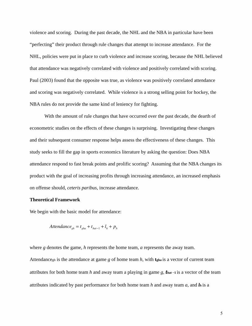
We begin with the basic model for attendance:

where g denotes the game, h represents the home team, a represents the away team.

Attendancegh is the attendance at game g of home team h, with tgha is a vector of current team

attributes for both home team h and away team a playing in game g, that 1 is a vector of the team

attributes indicated by past performance for both home team h and away team a, and lh is a

Attendancegh= t

gha+ t

hat 1+ l

h+ p

h

5

vector of the location attributes of the home team h, and ph denotes the price charged by the

home team h. Because the quality of game g is unknown, it is the expected quality of game g

based on previous performance captured by tgha. The term tgha represents many qualities of a

basketball game, including fast break points per game, total points per game, as well as their

current success in winning games.

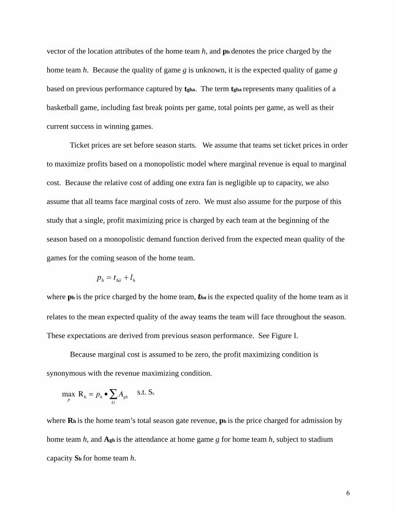
Ticket prices are set before season starts. We assume that teams set ticket prices in order

to maximize profits based on a monopolistic model where marginal revenue is equal to marginal

cost. Because the relative cost of adding one extra fan is negligible up to capacity, we also

assume that all teams face marginal costs of zero. We must also assume for the purpose of this

study that a single, profit maximizing price is charged by each team at the beginning of the

season based on a monopolistic demand function derived from the expected mean quality of the

games for the coming season of the home team.

where ph is the price charged by the home team, tha is the expected quality of the home team as it

relates to the mean expected quality of the away teams the team will face throughout the season.

These expectations are derived from previous season performance. See Figure I.

Because marginal cost is assumed to be zero, the profit maximizing condition is

synonymous with the revenue maximizing condition.

s.t. Sh

where Rh is the home team’s total season gate revenue, ph is the price charged for admission by

home team h, and Agh is the attendance at home game g for home team h, subject to stadium

capacity Sh for home team h.

ph = tha + lh

maxp

Rh= ph • Agh

G

6

Existing sports economics literature states that econometric analysis of attendance often

yields the disturbing result of an upward sloping demand curve, which is blamed on an omitted

variable, as detailed in Fizel (2006). This conclusion fails to take into account what is modeled

when performing econometrics analysis of game-to-game attendance variation. Instead of

modeling demand and movements along the demand curve, econometric analysis of game-to-

game attendance variation actually models the price-quality schedule, where the shifts in the

demand curve identify the price-quality schedule. See Figures II and III for a graphical

representation.

Including home team fixed effects has many implications regarding the estimation

equation formulation. All the predetermined variables are captured with the home team fixed

effects, which includes previous season success (or failure) of the home team, locational

qualities, and ticket prices. Since we are not controlling for the away team, the fixed qualities of

the away team are included in the final estimation equation. In addition, it should be noted that

because of this approach, we are modeling the shifts in the demand function as a result of quality

variations over the course of the season. The changes in demand due to home team quality are

expected to be smaller, and possibly insignificant, due to the use of home team fixed effects.

Because the home team’s previous seasons’ quality and success are included in the fixed effect

terms and the fact that the largest change game to game is the opponent rather than the home

team quality, the home team’s variation is unlikely to be found significant. From this we find the

only remaining terms in the equation are:

Attendancegh= t

gha+ t

at 1+ FE

7

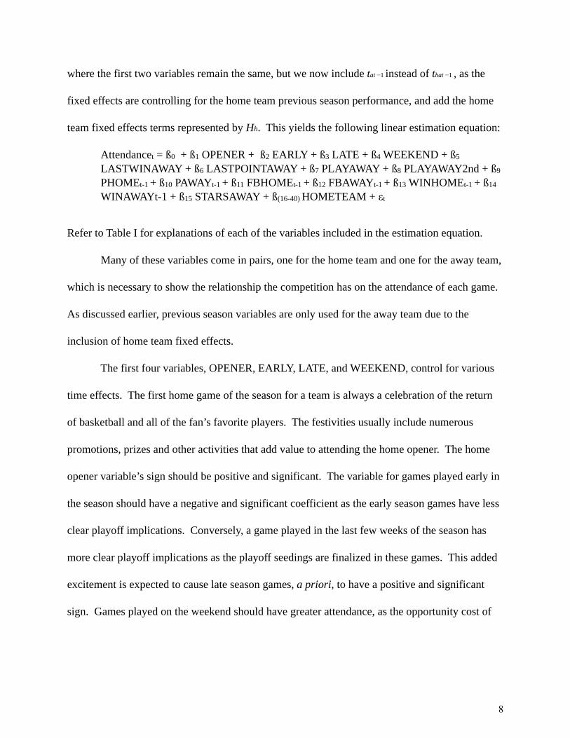
where the first two variables remain the same, but we now include tat 1 instead of that 1 , as the

fixed effects are controlling for the home team previous season performance, and add the home

team fixed effects terms represented by Hh. This yields the following linear estimation equation:

Attendancet = ß0 + ß1 OPENER + ß2 EARLY + ß3 LATE + ß4 WEEKEND + ß5

LASTWINAWAY + ß6 LASTPOINTAWAY + ß7 PLAYAWAY + ß8 PLAYAWAY2nd + ß9

PHOMEt-1 + ß10 PAWAYt-1 + ß11 FBHOMEt-1 + ß12 FBAWAYt-1 + ß13 WINHOMEt-1 + ß14

WINAWAYt-1 + ß15 STARSAWAY + ß(16-40) HOMETEAM + t

Refer to Table I for explanations of each of the variables included in the estimation equation.

Many of these variables come in pairs, one for the home team and one for the away team,

which is necessary to show the relationship the competition has on the attendance of each game.

As discussed earlier, previous season variables are only used for the away team due to the

inclusion of home team fixed effects.

The first four variables, OPENER, EARLY, LATE, and WEEKEND, control for various

time effects. The first home game of the season for a team is always a celebration of the return

of basketball and all of the fan’s favorite players. The festivities usually include numerous

promotions, prizes and other activities that add value to attending the home opener. The home

opener variable’s sign should be positive and significant. The variable for games played early in

the season should have a negative and significant coefficient as the early season games have less

clear playoff implications. Conversely, a game played in the last few weeks of the season has

more clear playoff implications as the playoff seedings are finalized in these games. This added

excitement is expected to cause late season games, a priori, to have a positive and significant

sign. Games played on the weekend should have greater attendance, as the opportunity cost of

8

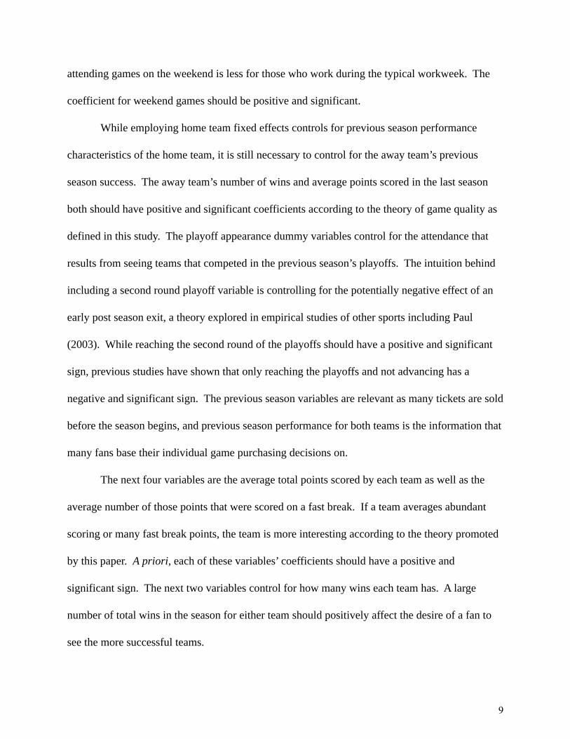
attending games on the weekend is less for those who work during the typical workweek. The

coefficient for weekend games should be positive and significant.

While employing home team fixed effects controls for previous season performance

characteristics of the home team, it is still necessary to control for the away team’s previous

season success. The away team’s number of wins and average points scored in the last season

both should have positive and significant coefficients according to the theory of game quality as

defined in this study. The playoff appearance dummy variables control for the attendance that

results from seeing teams that competed in the previous season’s playoffs. The intuition behind

including a second round playoff variable is controlling for the potentially negative effect of an

early post season exit, a theory explored in empirical studies of other sports including Paul

(2003). While reaching the second round of the playoffs should have a positive and significant

sign, previous studies have shown that only reaching the playoffs and not advancing has a

negative and significant sign. The previous season variables are relevant as many tickets are sold

before the season begins, and previous season performance for both teams is the information that

many fans base their individual game purchasing decisions on.

The next four variables are the average total points scored by each team as well as the

average number of those points that were scored on a fast break. If a team averages abundant

scoring or many fast break points, the team is more interesting according to the theory promoted

by this paper. A priori, each of these variables’ coefficients should have a positive and

significant sign. The next two variables control for how many wins each team has. A large

number of total wins in the season for either team should positively affect the desire of a fan to

see the more successful teams.

9

Also included is a variable for the presence of All-Star3 players on the away team. This

effect is captured by including a variable for the number of All Star players on each team plus

one. Theory and previous research suggest this variable will have a positive coefficient, as the .

more “star power” playing in the game, the better the quality of the game.

Summary Statistics

Data for the 2005-2006 NBA season contain observations for each of the 1,230 games

played during the regular season by the 30 teams in the NBA, all of which were entered

manually using box scores provided by the National Basketball Association on NBA.com4. .

The 2004-2005 season results used for previous season performance variables and the number of

All- Star players on each team were compiled from information provided by the National

Basketball Association, also available on NBA.com. I entered the data myself.

Two major changes were made to the data set to produce more accurate results. After

Hurricane Katrina, the New Orleans Hornets moved their home games to Oklahoma City’s Ford

Center. Midway through the season, the Hornets played six games in Louisiana including one in

Baton Rouge. This creates an inconsistency when attempting to control for home team fixed

effects, which would vary depending on where the game is played. The New Orleans/Oklahoma

City Hornets’ home games were excluded from the final data set. Teams that sell out every game

of the season, the Detroit Pistons, the Sacramento Kings and the San Antonio Spurs, lack of

variation in the dependent variable, which is necessary to produce accurate regression results.

These teams’ home games are also excluded from the data set.

3 An All-Star is defined as a player selected to be on the roster for either the Eastern Conference All-Star Team or the Western Conference All-Star Team. The starting 5 players for each team are voted for by fans, while the remaining 7 slots on each team are devoted to players chosen by the coach of each All-Star team.

4 Some observations had data missing from the box score, which were filled in by referencing an alternate databasehosted by ESPN.com.

10

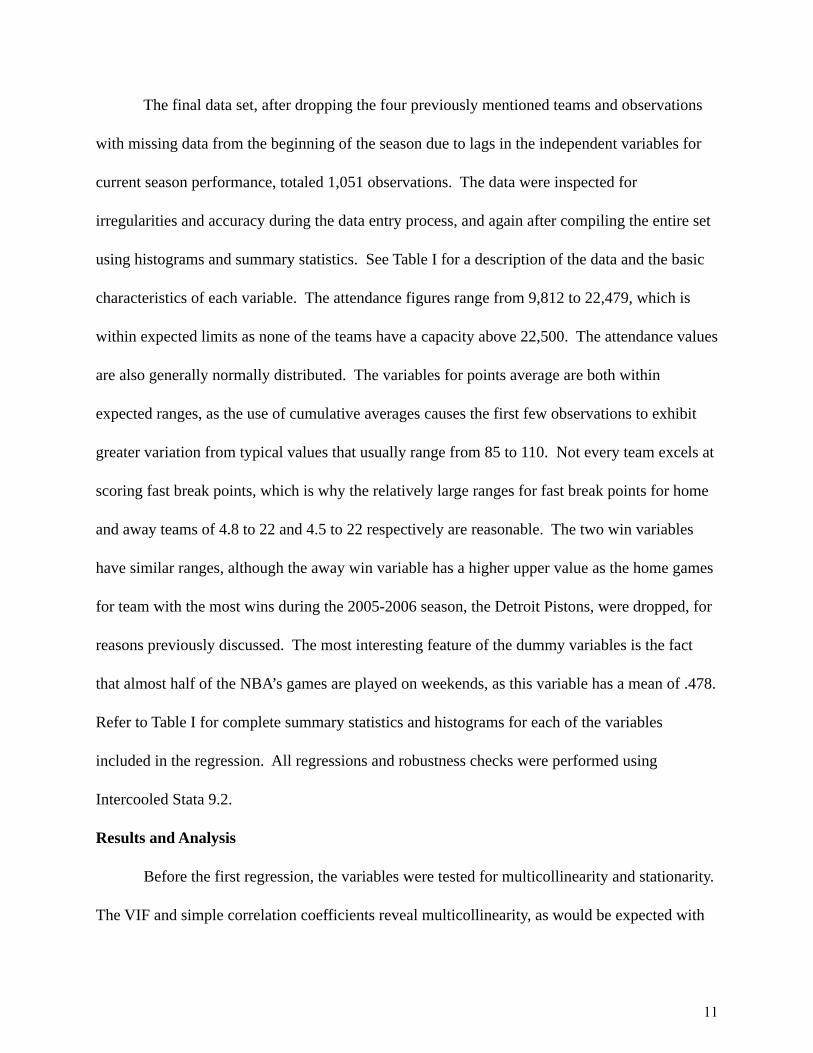
The final data set, after dropping the four previously mentioned teams and observations

with missing data from the beginning of the season due to lags in the independent variables for

current season performance, totaled 1,051 observations. The data were inspected for

irregularities and accuracy during the data entry process, and again after compiling the entire set

using histograms and summary statistics. See Table I for a description of the data and the basic

characteristics of each variable. The attendance figures range from 9,812 to 22,479, which is

within expected limits as none of the teams have a capacity above 22,500. The attendance values

are also generally normally distributed. The variables for points average are both within

expected ranges, as the use of cumulative averages causes the first few observations to exhibit

greater variation from typical values that usually range from 85 to 110. Not every team excels at

scoring fast break points, which is why the relatively large ranges for fast break points for home

and away teams of 4.8 to 22 and 4.5 to 22 respectively are reasonable. The two win variables

have similar ranges, although the away win variable has a higher upper value as the home games

for team with the most wins during the 2005-2006 season, the Detroit Pistons, were dropped, for

reasons previously discussed. The most interesting feature of the dummy variables is the fact

that almost half of the NBA’s games are played on weekends, as this variable has a mean of .478.

Refer to Table I for complete summary statistics and histograms for each of the variables

included in the regression. All regressions and robustness checks were performed using

Intercooled Stata 9.2.

Results and Analysis

Before the first regression, the variables were tested for multicollinearity and stationarity.

The VIF and simple correlation coefficients reveal multicollinearity, as would be expected with

11

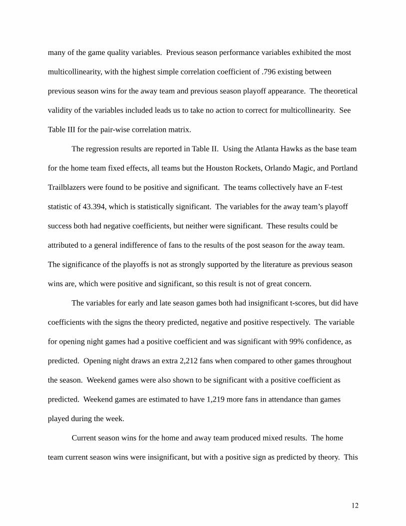
many of the game quality variables. Previous season performance variables exhibited the most

multicollinearity, with the highest simple correlation coefficient of .796 existing between

previous season wins for the away team and previous season playoff appearance. The theoretical

validity of the variables included leads us to take no action to correct for multicollinearity. See

Table III for the pair-wise correlation matrix.

The regression results are reported in Table II. Using the Atlanta Hawks as the base team

for the home team fixed effects, all teams but the Houston Rockets, Orlando Magic, and Portland

Trailblazers were found to be positive and significant. The teams collectively have an F-test

statistic of 43.394, which is statistically significant. The variables for the away team’s playoff

success both had negative coefficients, but neither were significant. These results could be

attributed to a general indifference of fans to the results of the post season for the away team.

The significance of the playoffs is not as strongly supported by the literature as previous season

wins are, which were positive and significant, so this result is not of great concern.

The variables for early and late season games both had insignificant t-scores, but did have

coefficients with the signs the theory predicted, negative and positive respectively. The variable

for opening night games had a positive coefficient and was significant with 99% confidence, as

predicted. Opening night draws an extra 2,212 fans when compared to other games throughout

the season. Weekend games were also shown to be significant with a positive coefficient as

predicted. Weekend games are estimated to have 1,219 more fans in attendance than games

played during the week.

Current season wins for the home and away team produced mixed results. The home

team current season wins were insignificant, but with a positive sign as predicted by theory. This

12

could be attributed to the use of home team fixed effects, which reduces the responsiveness of

the home team variables due to the fixed effects controlling for all previous season performance

variables. The away team’s wins were significant with a positive coefficient. Each additional

win of the away team increase attendance by almost 21 people.

The variables for offensive performance were mostly insignificant with mixed signs. The

home team’s fast break point and total point average both failed to reject the null hypothesis of a

coefficient equal to zero, as each had a negative and insignificant coefficient. Previous season

total points average for the away team was negative but insignificant. The away team’s average

total points for the current season were positive and significant, with approximately 49 more fans

attending the game for each point the away team averages. As the away team points average has

a mean of 96.30 and a standard deviation of 4.62, an away team that averages one standard

deviation from the mean in points per game, ceteris paribus, draws almost 250 more fans than an

away team that scores the mean. The away team’s fast break points had a negative sign, but

failed to reject the null hypothesis. The insignificance of the home and away team fast break

points suggests that the speed of the game does not have a statistically significant effect on

attendance.

The away team’s number of All-Stars was positive and significant with a 99% confidence

level. For each All-Star an away team’s roster, the game’s attendance goes up by more than 267.

For teams like the Miami Heat and the Phoenix Suns who have two All-Stars on their team,

attendance rises by nearly 535 fans. The Detroit Pistons, who had a record 4 All-Stars in

2005-2006, drew an estimated 1,068 more fans when playing on the road!

13

Robustness

The use of panel data presents a multitude of possible robustness deficiencies, with no

simple solutions in most cases. Because panel data span both time and space, it is important to

test for predominately cross sectional issues such as heteroskedasticity as well as predominately

time series issues such as serial correlation and stationarity. For the time series issues in

particular, testing each panel’s time series individually is an important step in checking the

robustness of the regression results.

Stationarity, primarily a time series problem, was tested for panel by panel for each

variable using the Dickey-Fuller test. Attendance rejected the null hypothesis of unit roots for

many of the panels, while the independent variables largely failed to reject the null hypothesis of

unit roots5. Due to this inconclusive result, the residuals were tested to check for stationarity in

the residual. None of the panels had non-stationarity issues in the residuals, which showed that

the variables are likely cointegrated. Cointegration made the use of first differences unnecessary.

After running the initial regression, the residuals were tested for serial correlation and

heteroskedasticity. Similar to the Dickey Fuller test, we used the Durban-Watson test repeated

for each panel to test for first order serial correlation. Because the panels were not ordered in a

meaningful way, we did not test for serial correlation across panels. All of the panels’ d-statistics

were within the inconclusive region6, failing to reject the null of no first order serial correlation.

We tested for heteroskedasticity using both the Breusch-Pagan and the White test, isolating a

single cross sectional unit, given that the proportionality factor is unknown. Both tests failed to

reject the null hypothesis of constant variance, providing evidence of homoskedasticity. The

5 The prolific nature of this approach makes the inclusion of these test outputs inappropriate.

14

evidence provided by these robustness tests suggests that the initial regression results are in fact

robust.

Conclusions and Directions for Further Research

This study estimated the impact of increased offense and speed in the NBA on

attendance. Using data from the 2005-2006 NBA season, this study found evidence of away

team points scored does have an economically significant effect on attendance, while game speed

as represented by fast break points does not have any significant effect on attendance.

It should be noted that this is not the end of the exploration of structural changes in the NBA.

This study focused on one structural change, while over the course of NBA history the institution

of rules like the 24-second shot clock and the three point line changed the rules of basketball

even more drastically than the changes explored in this paper. These changes warrant separate

studies from a more historical perspective. In addition, the functional form and specification

employed by this paper is by no means ideal, as the multicollinearity between points scored and

wins is necessarily high. One could instead eliminate this multicollinearity by employing a set of

variables to predict wins through points scored and other variables that determine the outcome of

a given game. This would have the added benefit of allowing for the maximization of attendance

through the principles presented by proponents of the Uncertainty of Outcome Hypothesis.

This study only examines a small element of the determinants of professional basketball’s

value and institutional renovations of professional basketball. More analysis of these topics

could help inform our understanding of consumer preferences for professional basketball and the

nature of leisure goods in general.

15

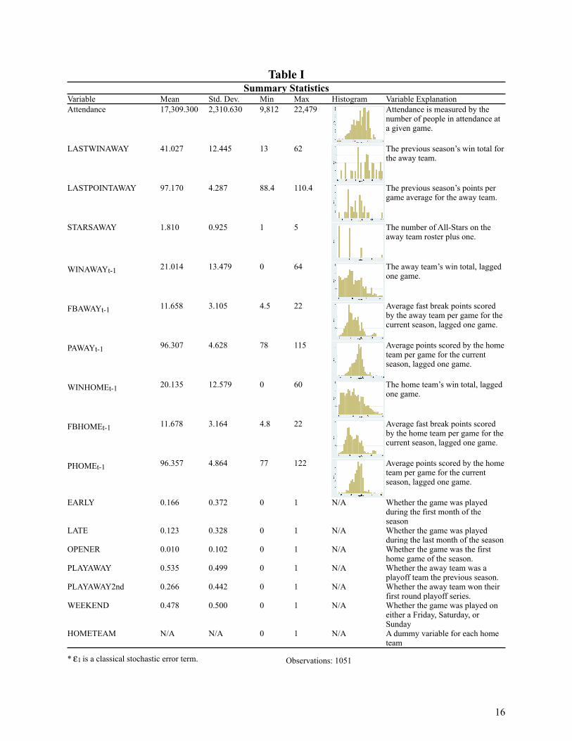
Table ISummary Statistics

Variable Mean Std. Dev. Min Max Histogram Variable ExplanationAttendance 17,309.300 2,310.630 9,812 22,479 Attendance is measured by the

number of people in attendance at a given game.

LASTWINAWAY 41.027 12.445 13 62 The previous season’s win total for the away team.

LASTPOINTAWAY 97.170 4.287 88.4 110.4 The previous season’s points per game average for the away team.

STARSAWAY 1.810 0.925 1 5 The number of All-Stars on the away team roster plus one.

WINAWAYt-1 21.014 13.479 0 64 The away team’s win total, lagged one game.

FBAWAYt-1 11.658 3.105 4.5 22 Average fast break points scored by the away team per game for the current season, lagged one game.

PAWAYt-1 96.307 4.628 78 115 Average points scored by the home team per game for the current season, lagged one game.

WINHOMEt-1 20.135 12.579 0 60 The home team’s win total, lagged one game.

FBHOMEt-1 11.678 3.164 4.8 22 Average fast break points scored by the home team per game for the current season, lagged one game.

PHOMEt-1 96.357 4.864 77 122 Average points scored by the home team per game for the current season, lagged one game.

EARLY 0.166 0.372 0 1 N/A Whether the game was played during the first month of the season

LATE 0.123 0.328 0 1 N/A Whether the game was played during the last month of the season

OPENER 0.010 0.102 0 1 N/A Whether the game was the first home game of the season.

PLAYAWAY 0.535 0.499 0 1 N/A Whether the away team was a playoff team the previous season.

PLAYAWAY2nd 0.266 0.442 0 1 N/A Whether the away team won their first round playoff series.

WEEKEND 0.478 0.500 0 1 N/A Whether the game was played on either a Friday, Saturday, or Sunday

HOMETEAM N/A N/A 0 1 N/A A dummy variable for each home team

* ε1 is a classical stochastic error term. Observations: 1051

16

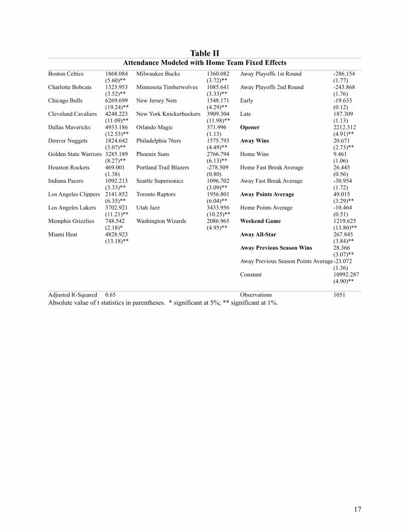
Table IIAttendance Modeled with Home Team Fixed Effects

Boston Celtics 1868.084 Milwaukee Bucks 1360.082 Away Playoffs 1st Round -286.154(5.60)** (3.72)** (1.77)

Charlotte Bobcats 1323.953 Minnesota Timberwolves 1085.641 Away Playoffs 2nd Round -243.868(3.52)** (3.33)** (1.76)

Chicago Bulls 6269.699 New Jersey Nets 1548.171 Early -19.633(19.24)** (4.29)** (0.12)

Cleveland Cavaliers 4248.223 New York Knickerbockers 3909.304 Late 187.309(11.09)** (11.98)** (1.13)

Dallas Mavericks 4933.186 Orlando Magic 371.996 Opener 2212.312(12.53)** (1.13) (4.91)**

Denver Nuggets 1824.642 Philadelphia 76ers 1575.793 Away Wins 20.671(3.07)** (4.49)** (2.73)**

Golden State Warriors 3285.189 Phoenix Suns 2766.794 Home Wins 9.461(8.27)** (6.13)** (1.06)

Houston Rockets 469.001 Portland Trail Blazers -278.509 Home Fast Break Average 26.445(1.38) (0.80) (0.56)

Indiana Pacers 1092.213 Seattle Supersonics 1096.702 Away Fast Break Average -30.954(3.33)** (3.09)** (1.72)

Los Angeles Clippers 2141.852 Toronto Raptors 1956.801 Away Points Average 49.015(6.35)** (6.04)** (3.29)**

Los Angeles Lakers 3702.921 Utah Jazz 3433.956 Home Points Average -10.464(11.21)** (10.25)** (0.51)

Memphis Grizzlies 748.542 Washington Wizards 2086.965 Weekend Game 1219.625(2.18)* (4.95)** (13.80)**

Miami Heat 4828.923 Away All-Star 267.845(13.18)** (3.84)**

Away Previous Season Wins 28.366(3.07)**

Away Previous Season Points Average-23.072(1.36)

Constant 10992.287(4.90)**

Adjusted R-Squared 0.65 Observations 1051Absolute value of t statistics in parentheses. * significant at 5%; ** significant at 1%.

17

Attendance PLAYAWAY PLAYAWAY2nd EARLY LATE OPENER WINAWAYt-1 WINHOMEt-1

Attendance 1

PLAYAWAY 0.1278 1

PLAYAWAY2nd 0.1177 0.5656 1

EARLY -0.0681 -0.0182 -0.0029 1

LATE 0.1024 -0.01 -0.0227 -0.1722 1

OPENER 0.0901 -0.0104 0.0419 0.3406 -0.0587 1

WINAWAYt-1 0.1892 0.2201 0.2496 -0.5767 0.4657 -0.2304 1

WINHOMEt-1 0.2458 -0.0149 -0.0295 -0.5866 0.5043 -0.2358 0.7521 1

FBHOMEt-1 0.0904 0.0008 -0.0025 0.023 0.0101 0.0251 -0.0138 0.1344

FBAWAYt-1 0.0228 0.1391 0.1929 -0.017 0.0081 0.0686 0.1129 -0.0087

PAWAYt-1 0.1307 0.2951 0.3801 -0.1053 0.0507 0.0149 0.2347 0.1017

PHOMEt-1 0.2803 0.0122 0.0092 -0.014 0.049 0.0097 0.0621 0.2038

WEEKEND 0.2152 0.0208 -0.0221 -0.0049 -0.0101 -0.0517 -0.0099 -0.0345

STARSAWAY 0.2037 0.4566 0.5534 -0.0163 -0.0088 -0.0259 0.2835 -0.0146

LASTWINAWAY 0.176 0.7963 0.6343 -0.0386 -0.0177 -0.0284 0.3055 0.0008

LASTPOINTAWAY 0.0741 0.2915 0.3128 -0.0736 -0.009 0.0245 0.1098 0.037

FBHOMEt-1 FBAWAYt-1 PAWAYt-1 PHOMEt-1 WEEKEND STARSAWAY LASTWINAWAYLASTPOINTAWAY

FBHOMEt-1 1

FBAWAYt-1 -0.0514 1

PAWAYt-1 -0.0489 0.5814 1

PHOMEt-1 0.5806 -0.0165 0.011 1

WEEKEND -0.0263 0.0241 -0.0094 -0.0038 1

STARSAWAY -0.0031 0.0388 0.2755 0.0149 0.0121 1

LASTWINAWAY 0.0001 0.1356 0.3796 0.007 -0.0052 0.6282 1

LASTPOINTAWAY -0.0206 0.3177 0.5755 -0.019 -0.0336 0.17 0.5526 1

Table III

18

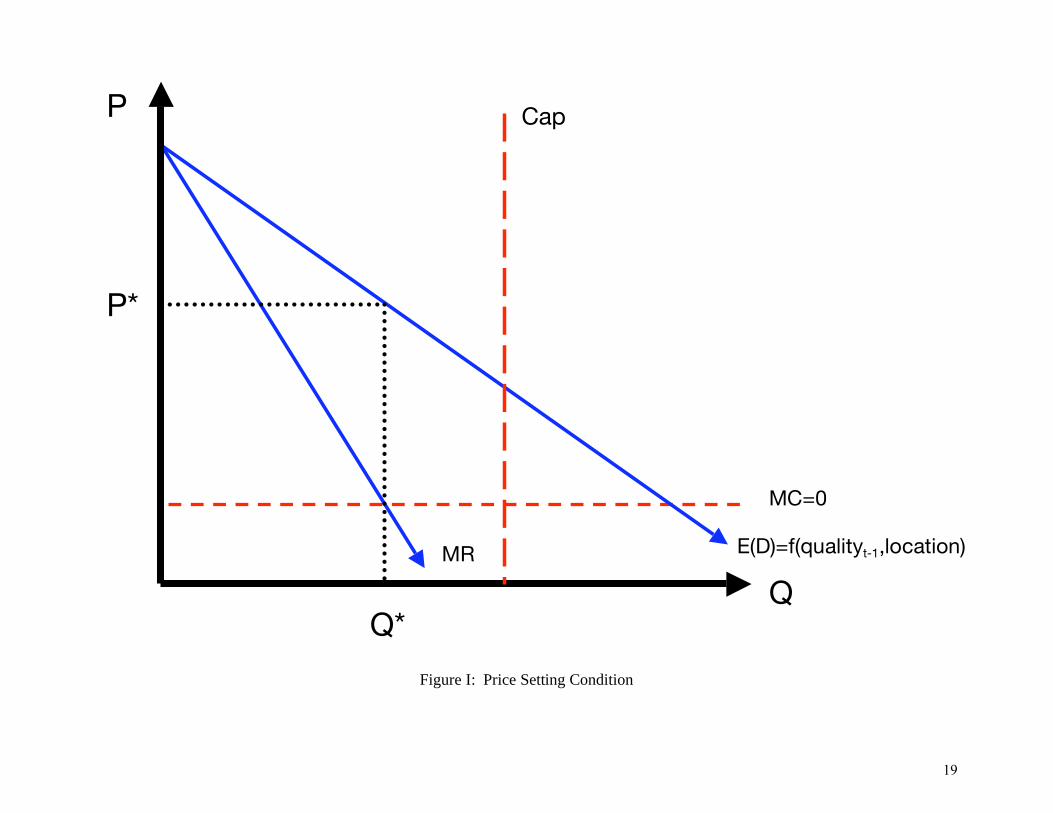
Figure I: Price Setting Condition

Q

P

MR

MC=0

E(D)=f(qualityt-1,location)

P*

Q*

Cap

19

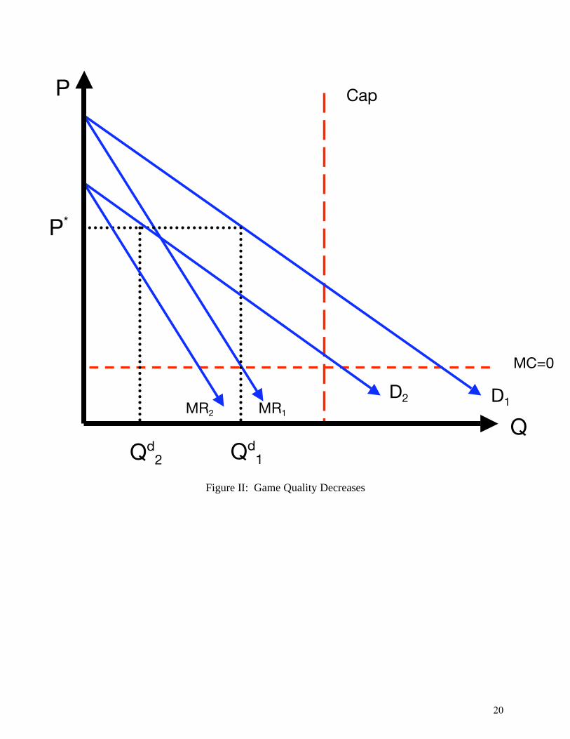
Figure II: Game Quality Decreases

Q

P

MR1

MC=0

D1

P*

Qd1

Cap

MR2 D2

Qd2

20

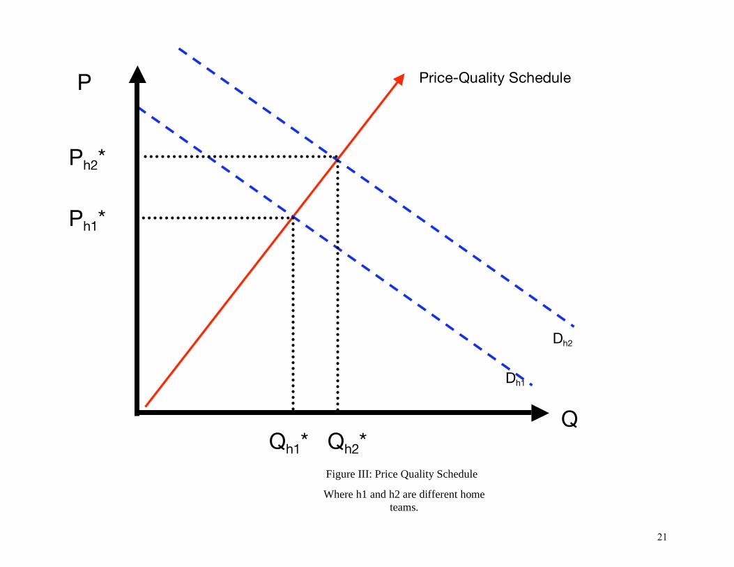
Figure III: Price Quality Schedule

Q

P

Dh1

Ph1*

Qh1*

Ph2*

Qh2*

Dh2

Price-Quality Schedule

Where h1 and h2 are different home

teams.

21

References

Berri, D. J., & Schmidt, M. B. (2006). On the road with the national basketball association's superstar externality. Journal of Sports Economics, 7(4), 347-358.

Berri, D. J., Schmidt, M. B., & Brook, S. L. (2004). Stars at the gate: The impact of star power on NBA gate revenues. Journal of Sports Economics, 5(1), 33-50.

Dupree, D. (2006, January 24). Next up, 100? Strategies, rule changes make it a possibility. USA Today, Retrieved from http://www.usatoday.com/sports/basketball/nba/2006-01-23-100-points_x.htm

Eifling, S. (2003, June 16). The 7-foot square: Why you don't love Tim Duncan. Article posted to http://www.slate.com/id/2094433/

Fizel, J. (Ed.). (2006). Handbook of sports economics research. Armonk, New York: M.E. Sharpe.

Hausman, J, & Leonard, G. (1997). Superstars in the national basketball association: Economic value and policy. Journal of Labor Economics, 15(4), 586.

Neale,W.C . (1964). The peculiar economics of professional sports. The Quarterly Journal of Economics, 78(1), 1.

Paul, R. (2003). Variations in NHL attendance. The American Journal of Economics and Sociology, 62(2), 345.

Rottenberg, S. (1956). The baseball players' labor market. The Journal of Political Economy, 64(3), 242.

Whitney, J. (1988). Winning games versus winning championships: The economics of fan interest and team performance. Economic Inquiry, 26(4), 703.

Data Set

National Basketball Association. (2006). Team and season statistics for 2004-2005 and 2005-2006 seasons: National Basketball Association. Retrieved on March 14, 2008. http://www.nba.com/.

National Basketball Association. (2006). Team and season statistics for 2004-2005 and 2005-2006 seasons: National Basketball Association. Retrieved on March 14, 2008. http://sports.espn.go.com/nba/index/.

22