Does Money Illusion Delude Investors? Evidence from Anomalies

By

Yuna Heo*

School of Accounting and Finance

The Hong Kong Polytechnic University

Hong Kong

* School of Accounting and Finance, The Hong Kong Polytechnic University, Hong Kong. Email:

yuna.heo@polyu.edu.hk

Does Money Illusion Delude Investors? Evidence from Anomalies

Abstract

This paper investigates the role of money illusion in the anomaly-based strategies. To the extent

that anomalies reflect mispricing, I examine whether money illusion predicts anomaly returns. I

find that, following high inflation, anomalies are stronger and the returns on the short-leg

portfolios are lower. These findings indicate that money illusion leads to mispricing in the stock

market. I explore the source of money illusion-driven mispricing. I find that money illusion

negatively predicts forecast errors and dispersion. These results suggest that investors

overestimate the upside potential of stock returns following high inflation and are subsequently

surprised by the return reversal.

JEL Classification: G02, G12, E31

Key words: Money Illusion, Inflation, Anomalies, Mispricing

1

1. Introduction

Whether the inflation, namely money illusion, affects stock prices is a question of long-

standing interest to researchers. As early as Fisher (1928) defines money illusion as “the failure

to perceive that the dollar, or any other unit of money, expands or shrinks in value”, numerous

papers have examined the existence of money illusion in the equity market. In early works,

equities had often been regarded as a claim against physical assets whose real returns remain

unaffected by inflation.1 However, contrary to the conventional view, many empirical studies

find a negative relation between inflation and stock returns.2

In recent years, many papers have documented the renewed interests in the existence of

money illusion in the capital market. For example, Cohen, Polk, and Vuolteenaho (2005) revisit

the issue of money illusion and provide a strong support for Modigliani and Cohn (1979)

hypothesis.3 Brunnermeier and Julliard (2008) find that housing market trends are largely

explained by variations in the inflation.4 These recent studies suggest that money illusion

possibly leads to mispricing in the stock market. In this paper, motivated by controversial

findings in earlier works and recent renewed interests in money illusion, I investigate the role of

money illusion in the stock market by testing anomaly returns.

1 Many researchers thought that the Fisher (1930) hypothesis that a nominal interest rate fully reflects the

available information concerning the future values of the rate of inflation might also hold for the stock

return-inflation relation. Regarding this, Tobin (1972) described: “An economic theorist can, of course,

commit no greater crime than to assume money illusion”. See Fehr and Tyran (2001) for the detailed

discussion. 2 For example, see Bodie (1976), Jaffe and Mandelker (1976), Nelson and Schwert (1977), Fama and

Schwert (1977), Gultekin (1983), Modigliani and Cohn (1979) Kaul (1987, 1990), and Kaul and Seyhun

(1990). 3 Modigliani and Cohn (1979) propose the hypothesis that stock market investors are subject to inflation

illusion. Modigliani and Cohn (1979) assume that the valuations of the assets differ from their

fundamental values because of two inflation-induced errors in judgments. 4 In addition, Sharpe (2002), Ritter and Warr (2002), Campbell and Vuolteenaho (2004), Chen, Lung, and

Wang (2009), Lee (2010), Birru and Wang (2014), and Warr (2014) have studies the effect of money

illusion in the capital market.

2

The objective of this paper is to examine whether money illusion plays an important role

in affecting the degree of mispricing in the stock market. At the simplest level, money illusion

occurs when investors mix real growth rates with nominal discount rates. This valuation error

can induce significant impacts in the stock prices. The key explanation of money illusion effects

is that, following high inflation periods, money-illusioned investors are overly optimistic for the

past performance of equities and excessively extrapolate into the future when they value firms.

To the extent that firms‟ stock price can reflect the views of investors who are most optimistic, a

presence of money-illusioned investors can cause a stock price departs from its fundamental

value.

I start by testing the relation between money illusion and stock market returns to explore

the role of money illusion in the stock market. Consistent with the findings in previous literatures,

I find that the money illusion is a negative predictor for stock market returns during the period of

1965-2010. The magnitude of predictability is statistically significant and economically large. In

the univariate regression, I find that a one standard deviation increase in money illusion is

associated with about 0.5% decline in one month-ahead market returns. In the multivariate

regressions, I control for three predictive variables related interest rates and find that the effect of

money illusion remains significantly negative.5 These findings suggest that investors may

overestimate the upside potential of stock returns following high inflation periods and

subsequently experience negative returns.

To examine whether money illusion leads to mispricing, I entertain the possibility that

anomalies at least partially reflect mispricing in the stock market. In previous studies, Stambaugh,

Yu, and Yu (2012) explore the role of investor sentiment in a broad set of anomalies in cross-

5 The three predictive variables are: T-bill is the 3-month T-bill rate. Term is the difference between yield

on 10-year bond and the T-bill. Default is the difference between Baa and Aaa-rated corporate bonds.

3

sectional stock returns.6 Similar to Stambaugh, Yu, and Yu (2012), I investigate the role of

money illusion in the stock market by examining the anomaly-based strategies associated with

mispricing. I consider 11 well-documented anomalies in the previous literatures. Theses

anomalies include size, value (book-to-market equity), financial distress, net stock issues,

earnings quality, gross profitability, returns-on-assets (ROA), investment-to-assets, external

financing, and asset turnover. It is worthwhile to emphasize that, while this study shares a similar

setting with Stambaugh, Yu, and Yu (2012), I focus on the inflation to investigate whether

money illusion affects the degree of mispricing in the stock market.7 To the best of my

knowledge, this is the first paper to examine the relation between money illusion and anomaly

returns.

Two main empirical implications are tested to explore the role of money illusion in the

stock market. The first hypothesis is that anomalies are stronger following high inflation periods.

The first hypothesis indicates that the long-short spread should be larger following high inflation.

Consistent with the first hypothesis, I find that each of the long-short anomaly-based strategies

presents higher average returns following high inflation. In the predictive regressions, I find the

positive relation between money illusion and the long-short spread. These results imply that

mispricing is stronger following high inflation periods. The estimate of combination strategy on

the benchmark-adjusted returns presents that one standard deviation increase in money illusion is

associated with $0.0061 of an additional monthly profit in each long-short spread. Clearly, these

6 Stambaugh, Yu, and Yu (2012) combine the presence of market-wide sentiment with the Miller (1977)

short-sale argument. 7 Many fundamental mechanisms, including the divergence of opinions and short-sale constraints (Miller

(1977), Hong and Sraer (2012)) and sentiment (Baker and Wurger (2006), Stambaugh, Yu, Yuan (2012)),

can potentially lead to mispricing in the stock market. In this study, I simply use money illusion as a

proxy for mispricing.

4

findings suggest that money illusion plays an important role in affecting the degree of mispricing

in the stock market.

The second hypothesis is that stock returns on the short-leg portfolios should be lower

following high inflation. To the extent the anomaly reflects mispricing, the stocks in the short leg

should be relatively overpriced compared to the stocks in the long leg. This indicates that the

stocks in short leg should be more overpriced following high inflation, as a result, present lower

returns. Consistent with the second hypothesis, I find that the short leg of all anomaly-based

strategies presents lower excess returns following high inflation periods. The short leg of the

combined strategy earns 177 bps less per month following high inflation periods than low

inflation periods. In the predictive regressions, I find that the slope coefficients for the short-leg

returns of all anomalies are negative. These results suggest that investors overly extrapolate past

performance into the future when they value firms and subsequently experience negative returns.

The combination strategy implies that one standard deviation increase in money illusion is

related to 0.6% decrease in monthly excess return on the short-leg portfolio. These findings

clearly provide the evidence that money-illusioned investors overestimate the upside potential of

stock returns following high inflation periods.

To better understand the results of this study, I empirically investigate the possible source

of money illusion-driven mispricing. I examine two prominent explanations: the risk-based

explanation and the behavioral-based explanation. The risk-based explanation argues that the

omitted risk factor‟s premium may explain the required correlation with money illusion. The

behavioral-based explanation argues that investors excessively extrapolate on past performance

when they value firms and surprised by the subsequent return reversal. I examine the potential

for a risk-based explanation by controlling for an additional set of variables. I find that the effect

5

of money illusion remains largely unchanged: the predictive power of money illusion for

anomaly returns does not weaken after controlling for macro-variables and firm level predictive

variables.8 In addition, to access the potential for a behavioral-based explanation for previous

results, I examine the relation between money illusion and forecast errors and dispersion. I find

that money illusion negatively predicts forecast errors and dispersion. 9

The results indicate that

investors‟ ex-ante expectation of future performance was too optimistic and subsequently

surprised by the return reversal. This indicates that the behavioral-based explanation may support

the results of this study.

Lastly, I extend the exploration of money illusion effects by examining sentiment and

other commonly use measure for predicting stock returns. Many previous studies indicate that

sentiment captures market-wide impacts in the stock market.10

I control for the effect of

sentiment to investigate whether money illusion plays an additional role in cross-sectional stock

returns. I find that the effect of money illusion remains largely unchanged after controlling for

sentiment and many additional variables.11

The results suggest that money illusion can provide

the complementary power for cross-sectional stock returns beyond the commonly used variables.

Overall, this study contributes to the literatures on money illusion and mispricing by providing

novel evidence that money illusion can lead to mispricing in the stock market.

8 The variables are: T-bill as the 3-month T-bill rate, Term as the difference between yield on 10-year

bond and the T-bill, Default as the difference between Baa and Aaa-rated corporate bonds, the earnings-

to-price ratio, the dividend-to-price ratio, and the equity variance. 9 The results are consistent with the prediction of Stambaugh, Yu, and Yu (2012) that investors‟ views

must be sufficiently disperse to include rational valuation when sentiment is low. 10

For example, Baker and Wugler (2006) provide strong evidence that investor sentiment have significant

effects on the stock returns. Stambaugh, Yu, and Yu (2012) find evidence that anomaly returns are larger

following high levels of sentiment. 11

I control for an additional set of macro-related variables that seem reasonable to entertain as being

correlated with the risk premium. I control for yield premium, term premium, and default premium,

earnings-to-price ratio, the dividend-to-price ratio, and the equity variance.

6

This paper is organized as follows. Section 2 discusses related literatures and develops

hypotheses. Section 3 introduces data and presents descriptive statistics. Section 4 reports main

results. Section 5 investigates the source of money illusion-drive mispricing. Section 6 examine

whether money illusion provides the complementary power to explain the cross-sectional stock

returns. Section 7 concludes.

2. Related Literature and Hypothesis Development

2.1 Related Literature

Whether the inflation, namely money illusion, affects stock prices is a question of long-

standing interest to researchers. The concept of money illusion was analyzed in detail for the first

time by Fisher (1928). As Fisher (1928) defines money illusion as “the failure to perceive that

the dollar, or any other unit of money, expands or shrinks in value”, numerous papers have

examined the existence of money illusion in equity markets. Among many papers, it is worth

referring to the survey conducted by Shafir, Diamond, and Tverky (1997). Shafir, Diamond, and

Tverky (1997) find that money illusion is a persistent phenomenon among economic and non-

economic agents. In a same vein, Fehr and Tyran (2001) present that a presence of money-

illusioned agents can cause significant impacts in capital markets.

The relation between stock returns and inflation has been studied for many years.

Equities had traditionally been regarded as a hedge against inflation because equities are claims

against physical assets whose real returns should remain unaffected by inflation. Numerous

researchers thought that the Fisher (1930) hypothesis, which posit that a nominal interest rate

fully reflects the available information concerning the future values of the rate of inflation, might

also hold for the stock return-inflation relation. However, contrary to the conventional view and

7

the Fisher hypothesis, many empirical studies find a negative relation between inflation and real

stock returns.

There is an extensive literature documenting that realized returns are negatively

influenced by inflation. (See, for example, Bodie (1976), Jaffe and Mandelker (1976), Nelson

and Schwert (1977), Fama and Schwert (1977), and Gulteken (1983)) Several hypotheses have

been proposed to explain the observed negative relation between stock returns and inflation.12

Modigliani and Cohn (1979) propose the inflation illusion hypothesis that stock market investors

are subject to inflation illusion. Modigliani and Cohn (1979) assume that the valuations of the

assets differ from their fundamental values because of two inflation-induced errors in judgment.

To explain the inverse relation, Fama (1981, 1983) proposes the proxy hypothesis. The proxy

hypothesis suggests that a rise in expected inflation rationally induces investors to reduce

expected future real dividend growth prices and expected real discount rates, subsequently

lowers stock prices and realized returns. Later on, Amihud (1996) tests the relationship between

unexpected inflation and stock returns in Israel and conclude that his results support only the

proxy hypothesis explanation.

In recent years, several papers have documented the renewed interests in the existence of

money illusion, suggesting the possibility of money illusion-induced mispricing in capital

markets. For example, Ritter and Warr (2002) find that the bull market starting in 1982 was due

in part to equities being undervalued, whose cause is cognitive valuation errors of levered stocks

in the presence of inflation and mistakes in the use of nominal and real capitalization rates.

Campbell and Vuolteenaho (2004) revisit the issue of the stock price-inflation relation based on

12

Additionally, Geske and Roll (1983) and Kaul (1987) argue that the relationships are driven by links

between expected inflation and expected real economic performance. Feldstein (1980) proposes the tax

hypothesis to explain the inverse relation between higher inflation and lower share prices. Brandt and

Wang (2003) propose the time varying risk aversion hypothesis.

8

the time-series decomposition of the log-linear dividend yield model and provide strong support

for Modigliani and Cohn (1979) hypothesis.13

Cohen, Polk, and Vuolteenaho (2005) present

cross-sectional evidence supporting Modigliani and Cohn‟s hypothesis by simultaneously

examining the future returns of Treasury bills, safe stocks, and risky stocks. Cohen, Polk, and

Vuolteenaho (2005) find that money illusion causes the market‟s subjective expectation of the

equity premium to deviate systematically from the rational expectation.

Other recent studies about money illusion have examined earnings forecasts, bubbles,

dividend announcements and house prices. Sharpe (2002) find that analysts suffer from money

illusion in their forecasts. Chordia ans Shivakumar (2005) find that money illusion causes firms

whose earnings are positively related to inflation to be undervalued because investors fail to

incorporate the effect of inflation on the earnings growth rate. Focusing on asset bubbles, Chen,

Lung, and Wang (2009) find that while inflation illusion can explain the level of mispricing, it

does not explain the volatility of mispricing. Brunnermeier and Julliard (2008) test the effect of

the Modigliani and Cohn hypothesis on house prices and show that housing market trends are

largely explained by variations in the inflation, suggesting that home buyers suffer from inflation

illusion.

Given the discussion of numerous literatures, the impact on the economy and stock

returns arising from the effects of inflation are indisputable. Motivated by controversial findings

in earlier works and recent renewed interests in money illusion, I explore the role of money

illusion in the mispricing of stock returns and anomalies.

2.2 Hypotheses Development

13

Campbell and Vuolteenaho (2004) use the Campbell and Shiller (1988) valuation model to decompose

the dividend yield to examine the effect of inflation.

9

To test whether money illusion plays an important role in affecting the degree of

mispricing in the stock market, I entertain the possibility that anomalies at least partially reflects

mispricing related to money illusion. In previous studies, combining the impediments to short

selling as in Miller (1977), Stambaugh, Yu, and Yu (2012) explore the role of investor sentiment

in a broad set of anomalies in cross-sectional stock returns. Similar to Stambaugh, Yu, and Yu

(2012), I examine the relation between money illusion and its role in a broad set of anomaly-

based strategies.

Two main empirical implications are tested to investigate the effect of money illusion on

mispricing. The first implication is that mispricing should be stronger following high inflation.

At the simplest level, money illusion occurs when investors mix real growth rates with nominal

discount rates. This implies that a presence of money-illusioned investors can cause a stock price

depart from its fundamental value. The key explanation of money illusion effects is that,

following high inflation periods, money-illusioned investors are overly optimistic for the past

performance of equities and excessively extrapolate into the future when they value firms. This

valuation error can induce significant impacts in market prices in that a firm‟s stock price can

reflect the view of investors who are overly optimistic. In contrary, during low inflation periods,

the most optimistic views about stocks tend to be those of rational investors, and thus mispricing

during those periods is less likely. Therefore, the first hypothesis is that anomalies are stronger

following high inflation periods. This indicates that the long-short spread should be larger

following high inflation. The positive profit on each long-short strategy reflects the unexplained

cross-sectional difference in stock returns that constitutes an anomaly.

The second implication is that the stocks in short leg should be more overpriced

following high inflation. Stocks in short leg are relatively overpriced compared to the stocks in

10

the long leg. Specially, overpricing becomes more difficult to eliminate with impediments to

short selling. If the primary form of mispricing is overpricing, such overpricing can occur for

many stocks during high inflation periods. This implies that the stocks in short leg should be

more overpriced following high inflation. In this regard, the second hypothesis is that stock

returns on the short-leg portfolios should be lower following high inflation. This indicates that

investors may overestimate the upside potential of stock returns following high inflation periods

and subsequently experience negative returns.

It is worthwhile to emphasize that, while this study shares a similar setting with

Stambaugh, Yu, Yuan (2012), I focus on inflation to examine whether money illusion plays an

important role in affecting the degree of mispricing. Many fundamental mechanisms, including

the divergence of opinions and short-sale constraints (Miller (1977), Hong and Sraer (2011)) and

sentiment (Baker and Wurger (2006), Stambaugh, Yu, Yuan (2012)), can potentially lead to

mispricing in the stock market. In the current study, I simply use money illusion as a proxy for

mispricing.

3. Data

This section describes the data used in this study. I obtained the data from several sources.

I compile market returns and S&P 500 returns from CRSP. Four measures of stock market

returns are used: the value-weighted raw returns, the value-weighted excess returns, the S&P 500

raw returns, and the S&P excess return. The accounting information is obtained from

COMPUSTAT. The sample period is 1965 to 2010. I also conduct sub-sample analysis over

period 1970-1990 to ensure the robustness of results.

11

Inflation, namely money illusion, is defined as the change in Consumer Price Index (CPI)

from year t-1 to t,

Money Illusiont = (CPIt – CPIt-1)/CPIt-1

The data for CPI is obtained from the Bureau of Labor Statistics. Figure 1 plots money illusion

and CPI (Consumer Price Index) from 1965 and 2010. The inflation is relatively high and

volatile during 1970-1980. After 2000, the inflation is getting more volatile: The inflation peaked

in 2005 once and immediately plummeted. It reached a peak again in 2006 then it crushed in

2008.

Interest rates data including 10-year and 3-month Treasury bills are downloaded from

Federal Reserve Economic Data (FRED). I use three predictive variables related to interest rates.

I use the excess returns on an index of 10-year bonds issued by the U.S. treasury as a Term. I use

the excess returns on an index of investment grade corporate bonds as a Default. The one-period

change in the option adjusted credit spreads for Moody‟s Baa-rated corporate bonds is used as

the investment grade corporate bond rate. To compute excess returns, I use the three-month

Treasury bill (T-bill) rate as the risk-free rate.

3.1 Descriptive Statistics

Table 1 report the descriptive statistics for the market returns and inflation from 1965 to

2010. Panel A shows that money illusion has an average of 0.35% and a standard deviation of

0.36% monthly. Monthly average of the value-weighted raw return is 0.87% and the monthly

average of value-weighted excess returns is 0.43%, with standard deviations of 4.58% and 4.59%.

The monthly average raw return on S&P 500 is 0.59% and the excess returns is 0.14%, with

standard deviation of 4.42% and 4.43%. Panel B presents the correlations between stock market

12

returns and inflation. All correlations of stock market returns with inflation are negative and the

magnitudes are around -10%. This negative relation is consistent with the expected cross-

sectional correlation between stock market returns and money illusion.

4. Results

4.1 Univariate Regression

I run predictive regression of one-month-ahead market returns on inflation. Table 2

presents the results of univariate regressions. Panel A reports the results over the periods 1965-

2010 and Panel B reports the results over the sub-period 1970-1990. I use four measures of stock

market returns: the value-weighted raw returns, the value-weighted excess returns, the S&P 500

raw returns, and the S&P excess return. The independent variable, money illusion, is

standardized to have zero mean and unit variance, in order to interpret the economic significance

of the predictability.

I find that money illusion is a negative predictor of the stock market returns. The

magnitude is economically large: a one standard deviation increase in inflation is associated 0.53%

decline in one-month-ahead value-weighted excess returns. For returns on value-weighted raw

returns, the coefficient estimate is -0.42%. For returns on S&P 500, the slope estimates are larger

and still economically big: -0.56% for S&P 500 excess return and -0.45% for S&P 500 raw

return. Turing to Panel B, money illusion more significantly negatively predicts stock market

returns for the subsample period with adjusted R2 varying from 3.4% to 4.5%. The OLS

estimates on money illusion are -0.96 % for the value-weighted raw return and -1.05% for the

value-weighted excess return monthly. For Returns on S&P 500 excess return, the coefficients

are -0.99% for S&P raw return and -1.07% for S&P excess return monthly. In sum, Table 2

13

indicates that the relation between money illusion and stock market returns is consistently

negative.

4.2 Multivariate Regression

To examine whether money illusion has incremental power to predict market returns, I

include three predictive variables related to interest rates. The variables are: T-bill is the 3-month

T-bill rate. Term is the difference between yield on 10-year bond and the T-bill. Default is the

difference between Baa and Aaa-rated corporate bonds.

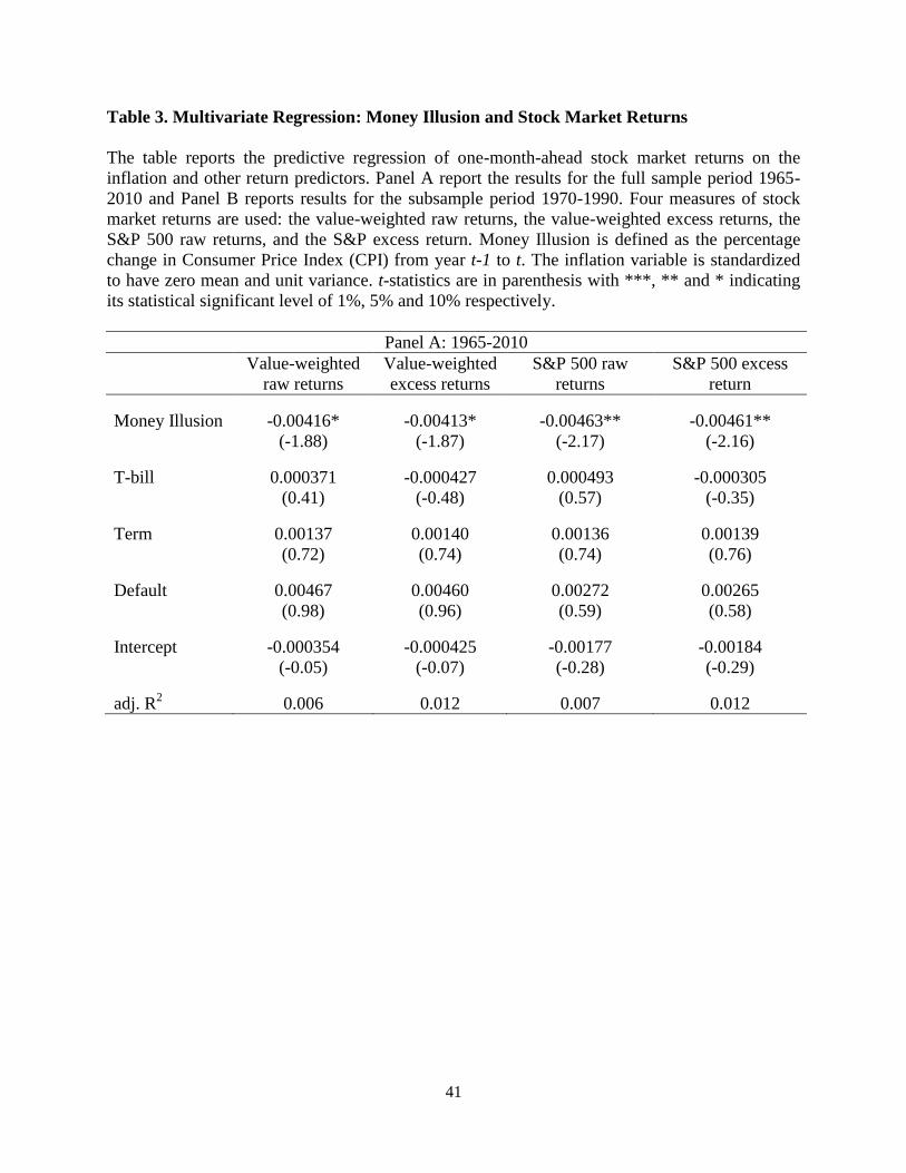
Table 3 presents the results of multivariate regressions. Panel A reports the results over

the periods 1965-2010 and Panel B reports the results over the sub-period 1970-1990. I use four

measures of stock market returns: the value-weighted raw returns, the value-weighted excess

returns, the S&P 500 raw returns, and the S&P excess return. The independent variable, money

illusion, is standardized to have zero mean and unit variance, in order to interpret the economic

significance of the predictability. I find that the estimates on money illusion remain negative and

significant. The magnitudes of the coefficient on money illusion are almost same in the

univariate regression: a one standard deviation increase in Inflation is associated with the 0.4%

decrease in one-month-ahead market returns. These results indicate that adding interest variables

has little effect on the ability of money illusion to predict returns. In Panel B, I perform sub-

period analysis. The results are similar. The adjusted R2 in the multivariate regressions ranges

from 8.9% to 10.1%, higher than those in the univariate regressions. In sum, money illusion

remains a negative predictor of stock market returns.

4.3 Money Illusion and Anomaly

14

I find that money illusion is a negative predictor for stock market returns during the

period of 1965-2010. These findings suggest that investors may overestimate the upside potential

of stock returns following high inflation periods. The key explanation of money illusion effects

is that, following high inflation periods, money-illusioned investors are overly optimistic for the

past performance of equities and excessively extrapolate into the future when they value firms.

This valuation error can induce significant impacts in market prices.

To test whether money illusion leads to mispricing in the stock market, I entertain the

possibility that anomalies at least partially reflect mispricing. In previous studies, Stambaugh, Yu,

and Yu (2012) explore the role of investor sentiment in a broad set of anomalies in cross-

sectional stock returns. Similar to Stambaugh, Yu, and Yu (2012), I examine the relation

between money illusion and anomaly-based strategies.

4.3.1 Anomaly- based Strategy

I consider 11 well-documented anomalies to explore the money illusion-driven

mispricing. Theses anomalies include size, value (book-to-market equity), financial distress, net

stock issues, earnings quality, gross profitability, ROA (return on assets), investment-to-assets,

external financing, and asset turnover. The explanation for each anomaly is as follows:

Size: Banz (1981) first documents the size effect by showing that small firms had higher risk-

adjusted returns than large firms during the 1936-1977 period. Essentially, this anomaly

indicates that small capitalization stocks outperform large capitalization stocks.

Value: Rosenberg, Reid, and Lanstein (1985) first suggest the value (book-to-market) strategy.

This strategy is well-described in Fama and French (1993) that high book-to-market firms

earn more than low book-to market firms.

15

Financial distress: Campbell, Hilscher, and Szilagyi (2008) find that firms with high financial

distress have lower subsequent returns. The failure probability (financial distress) is

estimated by a dynamic logit model with both accounting and equity market variables.

O-score: Ohlson (1980) O-score yields a similar anomaly to Campbell, Hilscher, and Szilagyi

(2008). Ohlson‟s O-score is measured by the probability of default in a static model using

various accounting variables.

Net stock issues: Pontiff and Woodgate (2008) present that there is a negative cross-sectional

relation between aggregate share issuance and stock returns. Fama and French (2008)

also present that net stock issuers earn negative realized returns.

Earnings quality: Sloan (1996) shows that firms with high accruals earn lower returns than firms

with low accruals. Total accruals are calculated as changes in noncash working capital

minus depreciation expense scaled by total assets.

Gross profitability: Novy-Marx (2013) finds that more profitable firms have higher returns than

less profitable firms. It is calculated by gross profits scaled by assets.

Return-on-assets: Chen, Novy-Marx, and Zhang (2011) show that firms with higher past return

on assets earn abnormally higher subsequent returns. Return on assets is measured by

earnings before extraordinary items scaled by assets.

Investment-to-assets: Titman, Wei, and Xie (2004) find that higher past investment predicts

abnormally lower future returns. Investment-to-assets is measured as the annual change

in gross property, plant, and equipment plus the annual change in inventories scaled by

the lagged book value of assets.

External financing: Bradshaw, Richardson, and Sloan (2006) find that net overall external

financing is negatively related to stock returns. This negative relation suggests that

16

investors may be relatively overoptimistic in forming their earnings expectations for high

net external financing firms. External financing is measured by as the net amount of cash a

firm raises from equity and debt markets.

Asset turnover: Novy-Marx (2013) find that high asset turnover firms have higher average

returns. Asset turnover is often regarded as a proxy of efficiency, which quantify the

ability to generate sales. Asset turnover is measured as sales-to-assets.

For each of the 11 anomalies, I examine the strategy that goes long the stocks in the

highest-performing decile and short the stocks in the lowest-performing decile. Every portfolio

formation on month, I sort stocks into the decile portfolios based on anomaly variables. I then

construct a long-short strategy using the extreme decile, 1 and 10, with the long leg being the

highest-performing decile and the short leg being the lowest-performing decile.

4.3.2 Anomaly Returns: High vs. Low Inflation

Table 4 presents excess monthly returns on a broad set of anomaly-based strategy

following high or low inflation periods. I fist classify returns on each month either a high

inflation period or a low inflation period. The high inflation period is one in which the value of

money illusion index in the previous month is above the median value for the sample period.

The low inflation period is the one below the median value.

The first hypothesis indicates that anomalies are stronger following high inflation periods.

This suggests that stocks should earn relatively low (high) returns following high (low) inflation

periods. Accordingly, the long-short spread should be larger following high inflation than low

inflation. The positive profit on each long-short strategy reflects the unexplained cross-sectional

difference in average returns that constitutes an anomaly. Table 4 clearly shows that the average

17

excess returns are lower following high inflation periods. All of the values in „High-Low‟

columns are negative and statistically significant. The last three columns in Table 4 present that

each of the long-short strategy shows higher average returns following high inflation. All of the

values in the last column are positive and statistically significant. The combined long-short

spread earns 123 bps per month following high inflation. These results imply that mispricing is

stronger following high inflation periods.

The second hypothesis indicates that the stocks in short leg should be more overpriced

following high inflation. To the extent that an anomaly reflects mispricing, the profits of the

long-short strategy represent relatively greater overpricing of stocks in the short leg. Thus,

according to the second hypothesis, the returns on the short leg are lower following high inflation

periods. In Table 4, the short leg of all anomaly strategies show a lower excess returns following

high inflation periods. All of the values are statistically significant and reject the null hypothesis

of no difference between high and low inflation periods. In Table 4, the short leg of the

combined strategy earns 177 bps less per month following high inflation periods than low

inflation periods. These results indicate that stocks in short leg are relatively overpriced

following high inflation. These findings suggest that investors may overestimate the upside

potential of stock returns following high inflation periods, inducing the money illusion-driven

overpricing.

Overall, the results in Table 4 provide strong support for the first hypothesis and the

second hypothesis. This evidence implies the possibility of money illusion-driven overpricing,

suggesting that investors excessively extrapolate past performance of stocks and are

subsequently experience negative returns.

18

4.3.3 Predictive Regression

Similar to Stambaugh, Yu, and Yu (2012), I use predictive regressions to examine

whether money illusion predicts anomaly returns. The first hypothesis predicts a positive relation

between the long-short spread and money illusion. Consistent with this prediction, the estimates

for the spreads are positive in both Table 5 and Table 6. In Table 5, ten of 11 anomalies are

statistically significant, and one of anomaly, which shows a negative prediction, is not significant.

The money illusion index is scaled to have zero mean and unit standard deviation. Therefore, the

slope coefficient of 0.0081 for the combination strategy indicates that one standard deviation

increase in money illusion is associated with $0.0081 of additional profit monthly on a long-

short strategy with $1 in each leg. In Table 6, ten of 11 anomalies are statistically significant.

The estimate of combination strategy indicates that one standard deviation increase in money

illusion is associated with $0.0061 of an additional monthly profit in each long-short spread.

The second hypothesis predicts a negative relation between the returns on the shot-leg

portfolio and the lagged money illusion level. Consistent with this prediction, the slope

coefficients for the short-leg returns of all anomalies are negative in both Table 5 and Table 6. In

Table 5, all t-statistics are significant. The combination strategy indicates that one standard

deviation increase in money illusion is associated with 0.8% decrease in monthly excess return

on the short-leg portfolio. In Table 6, ten out of 11 estimates are significant. The combination

strategy implies that one standard deviation increase in money illusion is related to 0.6%

decrease in monthly excess return on the short-leg portfolio.

In sum, results from predictive regressions reported in Table 5 and Table 6 suggest that

money illusion lead to overpricing in the stock market. Overall results are consistent with the

findings in Table 2 and Table 3 that investors overestimate the upside potential of stock returns

19

following high inflation periods. The key explanation is that, following high inflation periods,

money-illusioned investors are overly optimistic for the past performance of equities and

excessively extrapolate into the future when they value firms. These findings indicate money

illusion plays an important role in affecting the degree of mispricing in the stock market.

4.3.4 Alternative Money Illusion Index

Overall, the results support the empirical implication that high inflation induces

overpricing. This indicates that the money-illusioned investors are overly optimistic following

high inflation periods, as a result, produce grater mispricing effects on prices. An alternative

explanation for these results is that the money illusion index (i.e. the percentage change of

Consumer Price Index) by itself is asymmetric with the period of high inflation. Under this

explanation, the mispricing following high inflation periods simply reflect more strong inflation

effects during those periods. To address whether the results reflect pricing asymmetry or

inflation index asymmetry, I use the alternative measure of money illusion to examine the

anomaly returns.

Table 7 presents the results of regressions on the alternative money illusion index. The

alternative money illusion index is the inflation expectation, measured by median expected price

change next 12 months by Survey of Consumers. The data is obtained from FRED and the

source of data is from University of Michigan Inflation Expectation.14

The sample period is from

1978 to 2010. The alternative money illusion index is scaled to have zero mean and unit standard

deviation.

The alternative money illusion index show consistent implications with previous results.

In Table 7, ten of 11 anomalies are positive and eight of 11 anomalies are statistically significant.

14

Web address: http://research.stlouisfed.org/fred2/series/MICH

20

The estimate of combination strategy indicates that one standard deviation increase in money

illusion is associated with $0.0092 of an additional monthly profit in each long-short spread. The

results with the alternative money illusion index also support the second hypothesis that money

illusion is negatively associated with the returns on the shot-leg. In Table 7, all slope coefficients

for the short-leg returns are negative and seven of 11 anomalies are statistically significant. The

combination strategy indicates that one standard deviation increase in money illusion is

associated with 0.8% decrease in monthly excess return on the short-leg portfolio.

In sum, results from predictive regressions reported in Table 7 show consistent results

with Table 5 and Table 6, suggesting that previous results are not driven by asymmetry in

inflation index by itself. These results provide a strong support for the possibility of money

illusion-driven overpricing that money-illusioned investors overestimate the upside potential of

stock returns following high inflation periods.

5. A Source of Money Illusion-Driven Mispricing

In this section, I investigate the source of money illusion-driven mispricing by testing two

prominent explanations. The sources of money illusion-driven mispricing are two-fold: One is

based on risk and the other one is based on behavioral explanation. The risk-based explanation

argues that the stock returns reflect compensation for risk, indicating the risk premium would be

correlated with some aspect of macroeconomic conditions. The behavioral-based explanation

argues that investors excessively extrapolate on past performance when they value firms and

subsequently surprised by the negative returns.

5.1 Risk-Based Explanation

21

The risk-based explanation argues that the stock returns reflect compensation for risk,

indicating the risk premium would be correlated with some aspect of macroeconomic conditions.

It is challenging to explain why there is a difference in loadings between long and short legs. To

explain this difference, the risk-based explanation suggests the possibility of an omitted risk

factor to which each short leg is sensitive but each long leg is not. In this regard, the risk-based

explanation argues that the omitted risk factor‟s premium may explain the required correlation

with money illusion.

To access the potential for a risk-based explanation for previous results, I control for an

additional set of macro-related variables that seem reasonable to entertain as being correlated

with the risk premium. I control for yield premium, term premium, and default premium. The

yield premium is the 3-month T-bill rate. The term premium is the difference between yield on

10-year bond and the T-bill. The default premium is the difference between Baa and Aaa-rated

corporate bonds. Table 8 reports the results regressing excess returns on money illusion and

macro-variables. In Table 8, I find that nine of 11 anomalies are positive and statistically

significant. The estimate of combination strategy indicates that one standard deviation increase

in money illusion is associated with $0.0050 of an additional monthly profit in each long-short

spread. Also, slope coefficients for the short-leg returns are negative in eight out of 11 anomalies.

The combination strategy indicates that one standard deviation increase in money illusion is

associated with 0.28% decrease in monthly excess return on the short-leg portfolio.

I also control for firm level predictive variables in addition to macro-variables. The firm

level predictive variables are earnings-to-price ratio, the dividend-to-price ratio, and the equity

variance. Importantly, in Table 9, I find that the predictive power of money illusion for anomaly

returns does not weaken after I control for macro-variables and firm level predictive variables. In

22

Table 9, ten of 11 anomalies are positive and statistically significant. The estimate of

combination strategy indicates that one standard deviation increase in money illusion is

associated with $0.0042 of an additional monthly profit in each long-short spread. Also, slope

coefficients for the short-leg returns are negative in nine out of 11 anomalies and nine of 11

anomalies are statistically significant. The combination strategy indicates that one standard

deviation increase in money illusion is associated with 0.2% decrease in monthly excess return

on the short-leg portfolio.

To summarize the findings in Table 8 and Table 9, the results suggest that the effect of

money illusion remains largely unchanged after control for additional variables. The coefficient

and t-statistics are consistent with the main results in Table 5 and Table 6, in which the

additional variables are not included.

5.2. Behavioral-Based Explanation

The behavioral-based explanation argues that investors may overestimate the upside

potential of stock returns following high inflation periods, inducing the money illusion-driven

mispricing. The key explanation of money illusion effects is that, following high inflation

periods, money-illusioned investors are overly optimistic for the past performance of equities

and excessively extrapolate into the future when they value firms.

To access the potential for a behavioral-based explanation for previous results, I

investigate the relation between earnings forecast and money illusion. To examine the relation

between forecast errors and money illusion, I first obtain the 12-month-ahead target-price

forecasts for all individual analysts from the I/B/E/S database and aggregate the target-prices for

each calendar month. Then, I obtain the actual stock prices realized in 1-year from the CRSP

23

database, and define a variable forecast errors as the absolute value of the percentage difference

between the realized stock price and the 1-year-ahead target price forecast. In addition, I obtain

firms‟ financial accounting information from the COMPUSTAT database and calculate the log

total assets, financial leverage, market-to-book ratio, ROA, and R&D-to-asset ratio. This

approach is consistent with the analyst forecast literature.

I begin my analysis to fit regression specifications using forecast errors and money

illusion with year and month fixed effects. I control for other factors being documented in prior

research that can also influence analyst forecast behavior, such as firm size (log total assets),

profitability (ROA), leverage (asset to equity ratio), growth opportunity (market to book ratio),

and investment (R&D expense to asset ratio). Table 10 reports results of regressing forecast

errors on money illusion index. I break down the sample to two subsamples: high-performance

firms and low-performance firms. I find the negative coefficients on money illusion for the high-

performance firms. This result indicates that investors‟ ex-ante expectation of future performance

was too optimistic compared with the realized performance. Overall, results suggest that money-

illusioned investors tend to overestimate the upside potential of stock returns following high

inflation periods.

To clarify the role of dispersion in investors‟ views, I examine the relation between

forecast dispersion and money illusion. The forecast dispersion is defined as the standard

deviation of all analyst forecasts of 1-year-ahead target-price scaled by the average target-price

for each firm. Table 11 reports results of regressing forecast errors on money illusion index. I

find the negative coefficients on money illusion index. These results indicate that investors‟

views are more dispersed following low inflation. The results are consistent with the prediction

24

of Stambaugh, Yu, and Yu (2012) that investors‟ views must be sufficiently disperse to include

rational valuation when sentiment is low.

In sum, I find that money illusion negatively predicts forecast errors and forecast

dispersion. These results suggest that money-illusioned investors are overly optimistic for the

past performance of equities and excessively extrapolate into the future when they value firms.

6. Money Illusion, Sentiment, and Cross-Sectional Stock Returns

Overall, the results suggest that money-illisioned investors excessively extrapolate past

performance into future and are subsequently experience return reversal. These findings are

consistent with previous literatures by Delong, Shleifer, Summers, and Waldman (1990), Baker

and Wurgler(2007) and Stambaugh, Yu, and Yu (2012). In this section, I extend the exploration

of money illusion effects by examining sentiment and other commonly use measure for

predicting stock returns.

Baker and Wugler (2006) provide strong evidence that investor sentiment have

significant effects on the stock returns. Moreover, Stambaugh, Yu, and Yu (2012) find evidence

that anomaly returns are larger following high levels of sentiment. These previous studies

indicate that sentiment captures market-wide impacts in the stock market. Thus, to investigate

whether money illusion plays an important and complementary role in cross-sectional stock

returns, I control for the effect of sentiment first. The sentiment index is obtained from Baker and

Wurgler (2006). Table 12 reports results of regressing benchmark-adjusted anomaly returns on

money illusion index and Baker and Wugler sentiment index. The sentiment index is scaled to

have zero mean and unit standard deviation. The results in Table 12 are consistent with the

25

findings in Stambaugh, Yu, and Yu (2012). Each anomaly is stronger following high levels of

sentiment and is mainly due to the overpricing of short legs.

Importantly, focusing on the coefficient, b1, where money illusion is used as the

explanatory variable, I find that the predictive power of money illusion for anomaly returns does

not weaken after I control for the sentiment index. In Table 12, nine of 11 anomalies are positive

and statistically significant. The estimate of combination strategy indicates that one standard

deviation increase in money illusion is associated with $0.0073 of an additional monthly profit in

each long-short spread. Also, slope coefficients for the short-leg returns are negative in ten out of

11 anomalies and nine of 11 anomalies are statistically significant. The combination strategy

indicates that one standard deviation increase in money illusion is associated with 0.7% decrease

in monthly excess return on the short-leg portfolio. These results suggest that money illusion has

the complementary power for predicting anomaly performance, indicating that money illusion

provides new information beyond investor sentiment.

In addition to sentiment index, I control for an additional set of macro-related variables

that seem reasonable to entertain as being correlated with the risk premium. I control for yield

premium, term premium, and default premium. The yield premium is the 3-month T-bill rate.

The term premium is the difference between yield on 10-year bond and the T-bill. The default

premium is the difference between Baa and Aaa-rated corporate bonds. I also control for firm

characteristic variables. They are earnings-to-price ratio, the dividend-to-price ratio, and the

equity variance. Table 13 reports the results regressing excess returns on money illusion,

sentiment, macrovariables, and other firm characteristic variables. In Table 13, focusing on the

coefficient, b1, I find that nine of 11 anomalies are positive and statistically significant. The

estimate of combination strategy indicates that one standard deviation increase in money illusion

26

is associated with $0.0067 of an additional monthly profit in each long-short spread. Also, slope

coefficients for the short-leg returns are negative in nine out of 11 anomalies. The combination

strategy indicates that one standard deviation increase in money illusion is associated with 0.49%

decrease in monthly excess return on the short-leg portfolio.

In sum, the effect of money illusion remains largely unchanged after controlling for

sentiment and additional variables. These results suggest that money illusion plays an important

role in affecting the degree of mispricing in the stock market and provides the complementary

power to explain the cross-sectional stock returns.

7. Simple Model

In the presence of money illusion and short-sale constraints, the potential disagreement

between investors can lead overpricing. To the extent that judgment fallacies may affect some

investors but not others, or may differ across investors, heterogeneity of investor beliefs can be

sustained as an equilibrium phenomenon, and this in turn can affect asset prices in surprising

ways. One characteristic of the asset market is that different investors may interpret the same

information in different ways. Much of the public information such as inflation is subjective in

nature and open to different interpretations by investors. To better understand the interactions

among inflation, beliefs, and asset prices, I suggest a theoretical model that highlights

overpricing of stock returns.

7.1 Set up

This model is a simple variation on the Harrison and Kreps (1978) and Morris (1996)

model of speculative pricing in asset markets, where the key maintained assumption are risk

27

neutral investors, adequate liquidity, and short-selling constraints. To set up asset market to test

the theory of money illusion-driven overpricing, I impose short sales constraints and endow

investors with a lot of liquidity so that liquidity constraints do not bind.

7.2 Investors and Heterogeneous Beliefs

Assume that all investors use a common Bayesian updating rule, based on the true

stochastic process generating the signals. q is common knowledge and all investors update using

Bayes rule.

Let πt be the common posterior that the state of the world is A after St is revealed in

period t. 15 Given ρt, the common posterior if st = α is

πt ρt st = a =

qρt

qρt

+ 1 − q (1 − ρt)

and the common posterior if st = b is

πt ρt st = b =

(1 − q)ρt

(1 − q)ρt

+ q(1 − ρt)

Given that the asset pays off 1 in state A and 0 in state B, and given that all investors are

risk neutral, this common posterior at period t is also the valuation of the asset at period t. In this

15There are two possible states of the world, A and B. The probability of A being world is p. Nature

chooses the state of the world. There is an asset market with t+1 trading periods and i risk-neutral

investors. There is one type of asset in this market that pays off H per unit if A is the state of the world

and L(<H) per unit if B is the state of the world. Investors observe either a sequence of public signals, one

at the beginning of each trading period after the first. I assume the signals are generated by a stochastic

process that is independent across periods, conditional on the state. If ω = A, then st = a with probability

q>0.5 and st = b with probability 1-q. Likewise, when ω = B, st = b with probability q>0.5 and st = a

with probability 1-q. In the initial period, investors receive no information about the state of the world.

Since the asset pays off only in state A, I refer to a signal st = a as high inflation and a signal st = b as

low inflation.

28

model, each investor thinks her own belief is correct. Investors have own expectations about the

distribution of future prices, and disagree about the fundamental value of asset.

I consider a continuum of investor types characterized by the parameter θ ∈ [0, ∞]. An

investor with type θi will treat a public signal (i.e. inflation) as if it had the informational

equivalent of θ independent signals, each of informativeness q. Thus, θi measures how much

investor i under-react (θi < 1) or over-react (θi > 1) to the public signal, relative to q. Over-

reaction to signals is sometimes referred to neglect, and under-reaction is sometimes referred to

as conservatism.

Let πt be investor i‟s posterior that the state of world is A after st is revealed in period t.

This updated posterior after observing st = A for an investor of type θi is:

πitθi ρ

it st = A =

qθiρit

qθiρit

+ (1 − q)θi(1 − ρit

)

and after observing st = B is

πitθi ρ

it st = B =

(1 − q)θiρit

(1 − q)θiρit

+ qθi(1 − ρit

)

7.3 Equilibrium Price and Overpricing

I maintain the assumptions of binding short sale constraints and sufficient liquidity

among the investors to hold all the assets. Under these assumptions, I can apply the logic of the

Morris (1996) model to characterize the equilibrium price dynamics in our model. Given the way

I have defined different investors‟ types, and given that the initial prior belief is 0.5, the private

posterior and equilibrium prices will depend only on the investor types, the period number, t, and

the number of signals, h ≤ t. Thus, I can denote the current belief of investor type θi by

29

πitθi(h) =

qθ i h(1 − q)θ i (t−h)

qθ i h(1 − q)θi (t−h) + qθ i t−h (1 − q)θ i h

Define πt∗ h = maxi∈I{πit

θ i h } to be the most optimistic belief amongst the investors at

period t about A being the state of the world. The corresponding θ type for the investors with the

most optimistic belief is denoted θ∗. The price of the asset period t given the history of public

signals must be equal to the highest expect return of holding it to the next period t+1 in

equilibrium.

Let φt∗(h) be the most optimistic belief about the likelihood of good news being

announced in period t+1, after h good news signals and t-h bad news signals,

φt∗ h = πt

∗ h (qθ

∗

qθ∗

+ 1−q θ∗)+(1-πt

∗ h ( 1−q θ

∗

qθ∗

+ 1−q θ∗)

Note investors can only update their beliefs and asset valuations based on the sequence of

signals revealed so pricing depends upon the signals revealed and expectations about future

signals. The θ type with the most optimistic belief about the state of the world being A also has

the most optimistic belief about the next guess being A. Now I can specify the equilibrium price

Pt h = φt∗ h Pt+1 h + 1 + 1 − φ

t∗ h Pt+1(h + 1)

Therefore, I can define the speculate overpricing, αt h = Pt h − Pt∗(h). h is the number

of guesses about the high pay off state being realized. The speculative overpricing is the amount

by which the price exceeds the maximal valuation of all investors. This overpricing is the

different between the price and the most optimistic valuation. The price would reflect only the

belief of the most optimistic investor or possible exceed the valuations of all of the investors

when there is a speculative premium.

Recall that a continuum of investor types is characterized by the parameter θ ∈ [0,∞].

Following Morris (1996), I compare the price in each period to the investors‟ valuations and

30

derive several results. A permanent optimist has the highest probabilistic belief of A being the

state of the world out of all investors for every continuation sequence of signals (high inflation)

until the end of the market. Accordingly, speculate overpricing, αt h = Pt h − Pt∗(h), is the

amount by which the price exceeds the maximal valuation of all investors.

This implies that overpricing is more likely during high-inflation. The main prediction of

theoretical model is that, following high inflation periods, the most optimistic views about stocks

tend to be overly optimistic, as a result, stocks tend to be overpriced. In contrary, during low

inflation periods, the most optimistic views about stocks tend to be those of rational investors,

and thus overpricing during those periods is less likely. This would be consistent with the money

illusion-driven overpricing for the short portfolio stocks.

8. Conclusion

In this study, I investigate whether money illusion deludes investors, as a result, leads to

mispricing in the stock market. Numerous researches have examined the existence of money

illusion in the capital market and find that the impact of money illusion is crucial on the

economy. Motivated by early works and recent renewed interests in money illusion, I examine

whether inflation plays an important role in affecting the degree of mispricing in the equity

market.

To the extent that anomalies reflect mispricing, I test whether money illusion predicts

anomaly returns. I find that anomalies are stronger and the returns on the short-leg portfolio of

each anomaly are lower following high inflation periods. These findings indicate that money-

illusioned investors overestimate the upside potential of stock returns following high inflation

31

and subsequently experience the return reversal. To the best of my knowledge, this is the first

paper to examine the relation between money illusion and anomaly returns.

Furthermore, I explore the source of money illusion-driven mispricing. I find that money

illusion negatively predicts forecast errors and dispersion. The findings imply that, following

high inflation periods, investors are overly optimistic for the past performance of equities and

excessively extrapolate into the future when they value firms. This indicates that the behavioral-

based explanation may support the results of this study.

I extend the exploration of money illusion effects by examining sentiment and other

commonly use measure for predicting stock returns. I find that the effect of money illusion

remains largely unchanged after controlling for many additional variables. The results suggest

that money illusion can provide the complementary power for cross-sectional stock returns

beyond the commonly used variables. Overall, this study contributes to the literatures on money

illusion and mispricing by providing novel evidence that money illusion can lead to mispricing in

the stock market.

32

Reference

Amihud, Y., 1996, Unexpected inflation and stock returns revisited-Evidence from Israel,

Journal of Money, Credit, and Banking 28, 22-33.

Banz, Rolf., W., 1981, The relationship between return and market value of common stocks,

Journal of Financial Economics 9, 3-18.

Baker, M., Wurgler, J., 2007, Investor sentimentin the stock market, Journal of Economic

Perspective 21, 129-152.

Baker, M., Wurgler, J., 2006, Investor sentiment and the cross-section of stock returns, Journal

of Finance 61, 1645-1680.

Birru, Justin., Wang, Baolian, 2014, Nominal Price Illusion, Working paper, Ohio State

University.

Bodie, Z, 1976, Common stocks as a hedge against inflation, Journal of Finance 31, 459-470.

Bradshaw, Mark T., Scott A. Richardson, and Richard G. Sloan, 2006, The relation between

corporate financing activities, analysts‟ forecasts and stock returns, Journal of

Accounting and Economics 42, 53-85.

Brandt, M.W., Wang, K.Q., 2003, Time-varying risk aversion and unexpected inflation, Journal

of Monetary Economics 50, 1457-1498.

Brunnermeier, M., Julliard, C., 2008, Money Illusion and Housing Frenzies, Review of Financial

Studies 21, 135-180.

33

Cambell, J. Y., Hilscher, J., Szilagyi, J., 2008, In search of distress risk, Journal of Finance 63,

2899-2939.

Cambell, J. Y., Shiller, R., 1988, The dividend price ratio and expectation of future dividends

and discount factors, Review of Financial Studies 1, 195-227.

Campbell, J. Y., Vuolteenaho, T., 2004, Inflation illusion and stock prices, American Economic

Review 94, 19-23.

Chen, C., Lun, P., Wang, F., 2009, Stock market mispricing: Money illusion or the resale option,

Journal of Financial and Quantitative Analysis 44, 1125-1147.

Chen, L., Novy-Marx, R.,Zhang, L., 2011, An alternative three-factor model, Unpublished

working paper, University of Chicago.

Chordia, T., Shivakumar, L., 2005, Inflation illusion and post-earnings-announcement drift,

Journal of Accounting Research 43, 521-556.

Cohen, R., Polk, C., Vuolteenaho, T., 2005, Money illusion in the stock market: the Modigliani-

Cohn Hypothesis, Quarterly Journal of Economics 120, 639-668.

Delong, B., Shleifer, A., Summers, L. H., Waldmann, R., 1990, Noise trader risk in financial

market, Journal of Political Economy 90, 703-738.

Fama, E., 1983, Stock returns, real activity, inflation and money: reply, American Economic

Review 73, 471-472.

Fama, E., 1981, Stock returns, real activity, inflation and money, American Economic Review 71,

545-565.

34

Fama, E., French, K., 2008, Dissecting anomalies, Journal of Finance 63, 1653-1678.

Fama, E., French, K., 2006, Profitability, investment, and average returns, Journal of Financial

Economics 82, 491-518.

Fama, E., French, K., 1993, Common risk factors in the returns on stocks and bonds, Journal of

Financial Economics 33, 3-56.

Fama, E., Schwert, W., 1977, Asset returns and inflation, Journal of Financial Economics 5, 115-

146.

Fehr, earnst., Tyran, Jean-Robert., 2001, Does money illusion matter?, American Economic

Review 91, 1239-1262.

Feldstein, Martin, 1980, Inflation and the stock market, American Economic Review 70, 839-

847.

Fisher, I., 1928, The money Illusion, Adelphi, New York.

Fisher, I., 1930, The Theory of Interest, McMillan, New York.

Geske, R., Roll, R., 1983, The monetary and fiscal linkage between stock returns and inflation,

Journal of Finance 38, 1-33.

Glutekin, N. B., 1983, Stock market returns and inflation: Evidence from other countries, Journal

of Finance 38, 49-65

Hong, Harrison., Sraer, David., 2012, Speculative Betas, Working paper, Princeton University.

35

Jaffe, J. F., Mandelker, G., 1976, The „Fisher effect‟ for risky assets: An empirical investigation,

Journal of Finance 31, 447-458.

Kaul, G., 1987, Stock returns and inflation: the role of the monetary sector, Journal of Financial

Economics 18, 253-276.

Kaul, G., 1990, Monetary regimes and the relation between stock returns and inflationary

expectations, Journal of Financial Quantitative Analysis 25, 307-321.

Kaul, G., Seyhun, H.N., 1990, Relative price variability, real shocks, and the stock market,

Journal of Finance 45, 479-496.

Lee, Bong Soo., 2010, Stock returns and inflation revisited: An evaluation of the inflation

illusion hypothesis, Journal of Banking and Finance 34, 1257-1273.

Miller, E. M., 1977, Risk, uncertainty and divergence of opinion, Journal of Finance 32, 1151-

1168.

Modigliani, F., Cohn , R., 1979, Inflation, rational valuation, and the market, Financial Analysts

Journal 35, 24-44.

Nelson, C. R., Schwert, W., 1977, Short-term interest rates as predictors of inflation: On testing

the hypothesis that the real rate of interest is constant, American Economic Review 67,

478-486.

Novy-Marx, R., 2013, The other side of value: the gross profitability premium. Journal of

Financial Economics 108, 1-28.

36

Ohlson, J. A., 1980, Financial ratios and the probabilistic prediction of bankruptcy, Journal of

Accounting Research 18, 109-131.

Pontiff, J., Woodgate, A., 2008, Share issuance and the cross-section of returns, Journal of

Finance 63, 921-945.

Ritter, J.R., Warr, R.S., 2002, The decline of inflation and the bull market of 1982-1999. Journal

of Financial and Quantitative Analysis 37, 29-61.

Rosenberg, B, Reid, K., Lanstein, R., 1983, Persuasive evidence of market inefficiency, Journal

of Portfolio Management 11, 9-16.

Shafir, E., Diamond, P., Tverky, A., 1997, Money illusion, Quarterly Journal of Economics 62,

341-374.

Sharpe, S., 2002, Reexamining stock valuation and inflation: The implications of analyst‟s

earnings forecasts, Review of Economics and Statistics 84, 632-648.

Sloan, R. G., 1996, Do stock prices fully reflect information in accruals and cash flows about

future earnings? The Accounting Review 71, 289-315.

Stambaugh, Robert. F., Yu, Jianfeng., Yu, Yuan., 2012, The short of it: Investor sentiment and

anomalies, Journal of Financial Economics 104, 238-302.

Titman, S., Wei, K.C.J., Xie, F., 2004, Capital investments and stock returns. Journal of

Financial and Quantitative Analysis 39, 677-700.

Tobin, James., 1972, Inflation and Unemployment, American Economic Review 62, 1-18.

37

Warr, Richard. S., 2014, The effect of inflation illusion on the debt-equity choice, Working paper,

North Carolina State University.

38

Figure1. Money Illusion and CPI (Consumer Price Index)

This figure plots money illusion and CPI (Consumer Price Index) from 1965 and 2010. money

illusion is defined as the percentage change in CPI. The data for CPI is obtained from the Bureau

of Labor Statistics.

0

50

100

150

200

250

-2.5

-2

-1.5

-1

-0.5

0

0.5

1

1.5

2

19

65

19

66

19

68

19

70

19

72

19

74

19

76

19

78

19

80

19

82

19

84

19

86

19

88

19

89

19

91

19

93

19

95

19

97

19

99

20

01

20

03

20

05

20

07

20

09 Money Illusion

CPI

39

Table 1. Descriptive Statistics for Money Illusion and Stock Market Returns

The table reports the descriptive statistics for money illusion and stock market returns. Four

measures of stock market returns are used: the value-weighted raw returns, the value-weighted

excess returns, the S&P 500 raw returns, and the S&P excess return. Stock market returns are

computed monthly. Money illusion is defined as the percentage change in Consumer Price Index

(CPI) from year t-1 to t. The sample period is from 1965 to 2010.

Panel A: Descriptive Statistics

Variable Mean Std.dev Median

Money Illusion 0.0035 0.0036 0.0030

Value-weighted raw returns 0.0087 0.0458 0.0122

Value-weighted excess returns 0.0043 0.0459 0.0077

S&P 500 raw returns 0.0059 0.0442 0.0087

S&P 500 excess return 0.0014 0.0443 0.0048

Panel B: Correlation

Variable Value-

weighted raw

returns

Value-

weighted

excess

returns

S&P 500 raw

returns

S&P excess

return

Value-weighted raw returns 1

Value-weighted excess returns 0.9986 1

S&P 500 raw returns 0.9858 0.9844 1

S&P 500 excess return 0.9843 0.9858 0.9985 1

Money Illusion -0.0930 -0.1157 -0.1033 -0.1268

40

Table 2. Univariate Regression: Money Illusion and Stock Market Returns

The table reports the predictive regression of one-month-ahead stock market returns on the

inflation. Panel A report the results for the full sample period 1965-2010 and Panel B reports

results for the subsample period 1970-1990. Four measures of stock market returns are used: the

value-weighted raw returns, the value-weighted excess returns, the S&P 500 raw returns, and the

S&P excess return. Money illusion is defined as the percentage change in Consumer Price Index

(CPI) from year t-1 to t. The inflation variable is standardized to have zero mean and unit

variance. t-statistics are in parenthesis with ***, ** and * indicating its statistical significant

level of 1%, 5% and 10% respectively.

Panel A: 1965-2010

Value-weighted

raw returns

Value-weighted

excess returns

S&P 500 raw

returns

S&P 500 excess

return

Money Illusion -0.00426** -0.00531*** -0.00457** -0.00562***

(-2.19) (-2.73) (-2.44) (-3.00)

Intercepts 0.00873*** 0.00426** 0.00588*** 0.00142

(4.49) (2.19) (3.14) (0.76)

adj. R

2 0.007 0.012 0.009 0.014

Panel B: 1970-1990

Value-weighted

raw returns

Value-weighted

excess returns

S&P 500 raw

returns

S&P 500 excess

return

Money Illusion -0.00969*** -0.0105*** -0.00989*** -0.0107***

(-3.14) (-3.39) (-3.34) (-3.59)

Intercepts 0.0134*** 0.00759** 0.0103*** 0.00450

(4.09) (2.31) (3.27) (1.42)

adj. R

2 0.034 0.040 0.039 0.045

41

Table 3. Multivariate Regression: Money Illusion and Stock Market Returns

The table reports the predictive regression of one-month-ahead stock market returns on the

inflation and other return predictors. Panel A report the results for the full sample period 1965-

2010 and Panel B reports results for the subsample period 1970-1990. Four measures of stock

market returns are used: the value-weighted raw returns, the value-weighted excess returns, the

S&P 500 raw returns, and the S&P excess return. Money Illusion is defined as the percentage

change in Consumer Price Index (CPI) from year t-1 to t. The inflation variable is standardized

to have zero mean and unit variance. t-statistics are in parenthesis with ***, ** and * indicating

its statistical significant level of 1%, 5% and 10% respectively.

Panel A: 1965-2010

Value-weighted

raw returns

Value-weighted

excess returns

S&P 500 raw

returns

S&P 500 excess

return

Money Illusion -0.00416* -0.00413* -0.00463** -0.00461**

(-1.88) (-1.87) (-2.17) (-2.16)

T-bill 0.000371 -0.000427 0.000493 -0.000305

(0.41) (-0.48) (0.57) (-0.35)

Term 0.00137 0.00140 0.00136 0.00139

(0.72) (0.74) (0.74) (0.76)

Default 0.00467 0.00460 0.00272 0.00265

(0.98) (0.96) (0.59) (0.58)

Intercept -0.000354 -0.000425 -0.00177 -0.00184

(-0.05) (-0.07) (-0.28) (-0.29)

adj. R2 0.006 0.012 0.007 0.012

42

Panel B: 1970-1990

Value-weighted

raw returns

Value-weighted

excess returns

S&P 500 raw

returns

S&P 500 excess

return

Money Illusion -0.00643* -0.00642* -0.00696** -0.00695**

(-1.79) (-1.78) (-2.00) (-2.00)

T-bill -0.00448*** -0.00526*** -0.00425*** -0.00504***

(-2.70) (-3.18) (-2.66) (-3.15)

Term -0.00451 -0.00448 -0.00439 -0.00436

(-1.43) (-1.42) (-1.44) (-1.43)

Default 0.0374*** 0.0372*** 0.0340*** 0.0339***

(4.28) (4.27) (4.04) (4.02)

Intercept 0.00501 0.00493 0.00440 0.00433

(0.39) (0.39) (0.36) (0.35)

adj. R2 0.092 0.101 0.089 0.099

43

Table 4. Anomaly Returns: High vs. Low Inflation

This table reports excess monthly returns on a broad set of anomaly-based strategies. I classify

returns each month as following either a high-inflation or a low-inflation month. A high-inflation

month is one in which the value of the money illusion index in the previous month is above the

median value of sample period, and a low-inflation month is below the median values. t-statistics

are in parenthesis.

Anomaly Long leg Short leg Long-Short

High Low High-

Low High Low

High-

Low High Low

High-

Low

Size -0.0028 0.0004 -0.0032

(-3.19) 0.0080 0.0174

-0.0094

(-20.91)

-0.0108

(-16.59)

-0.0170

(-21.73)

0.0062

(6.07)

Book to Market -0.0181 -0.0145 -0.0036

(-4.56) -0.0110 0.0089

-0.0199

(-20.51)

-0.0071

(-9.22)

-0.0234

(-23.96)

0.0163

(13.02)

Financial Distress 0.0029 0.0055 -0.0026

(-2.60) 0.0150 0.0409

-0.0259

(-26.85)

-0.0121

(-13.36)

-0.0354

(-33.96)

0.0233

(16.90)

Ohlson‟s-O

(Distress) 0.0048 0.0112

-0.0065

(-19.88) -0.0213 0.0073

-0.0286

(-13.09)

0.0260

(33.41)

0.0039

(4.27)

0.0221

(17.91)

Net Stock Issues -0.0015 0.0079 -0.0094

(-32.59) 0.0029 0.0145

-0.0116

(-15.09)

-0.0044

(-8.20)

-0.0065

(-11.30)

0.0021

(2.70)

Accrual 0.0039 0.0098 -0.0059

(-11.11) 0.0044 0.0156

-0.0112

(-15.88)

-0.0005

(-0.83)

-0.0058

(-8.77)

0.0053

(5.91)

Profitability 0.0191 0.0276 -0.0085

(-10.61) -0.0154 0.0086

-0.0240

(-13.89)

0.0345

(30.47)

0.0190

(15.21)

0.0155

(9.05)

ROA 0.0170 0.0261 -0.0091

(-12.85) -0.0245 -0.0022

-0.0223

(-14.68)

0.0415

(42.03)

0.0283

(24.66)

0.0131

(8.66)

Investment-to-

assets 0.0059 0.0174

-0.0114

(-12.58) -0.0071 0.0086

-0.0157

(-12.98)

0.0130

(13.63)

0.0088

(7.70)

0.0092

(6.19)

External Finance 0.0069 0.0141 -0.0072

(-5.90) -0.0188 0.0052

-0.0240

(17.25)

0.0257

(20.88)

0.0089

(5.96)

0.0168

(8.71)

Asset Turnover 0.0041 0.0134 -0.0093

(-11.53) -0.0049 0.0169

-0.0218

(-10.88)

0.0090

(7.39)

-0.0034

(-2.60)

0.0124

(6.90)

Combination 0.0047 0.0096 -0.0049

(-8.45) -0.0031 0.0146

-0.0177

(13.21)

0.0078

(8.35)

-0.0050

(-4.53)

0.0128

(8.80)

44

Table 5. Predictive Regressions: Excess Returns on Long-Short Strategies

The table reports estimates of b in the regression

Ri,t = a + bMt-1 +et,

where Ri,t is the excess return in month t on either the long leg, the short leg, or the difference,

and Mt is the percentage of the money illusion index ((CPIt – CPIt-1)/CPIt-1). t-statistics are in

parenthesis.

Anomaly Long leg Short leg Long-Short

Size -0.0006

(1.14)

-0.0036

(-10.68)

0.0031

(5.93)

Book to Market -0.0032

(-8.33)

-0.0119

(-27.36)

0.0087

(14.11)

Financial Distress 0.0012

(2.39)

-0.0117

(-24.37)

0.0129

(18.85)

Ohlson‟s O (Distress) -0.0019

(-11.94)

-0.0146

(-24.34)

0.0127

(20.26)

Net Stock Issues -0.0049

(-33.15)

-0.0043

(-11.33)

-0.0006

(-1.60)

Accrual -0.0025

(-9.68)

-0.0051

(-16.65)

0.0026

(5.96)

Profitability -0.0027

(-6.46)

-0.1204

(-17.05)

0.0094

(10.37)

ROA -0.0044

(-12.49)

-0.0128

(-21.08)

0.0084

(10.81)

Investment-to-assets -0.0055

(-12.00)

-0.0083

(-15.41)

0.0028

(3.72)

External Finance -0.0030

(-5.13)

-0.0125

(-19.77)

0.0095

(10.00)

Asset Turnover -0.0047

(-11.70)

-0.0140

(-17.26)

0.0094

(10.04)

Combination -0.0003

(-0.84)

-0.0084

(-15.00)

0.0081

(10.34)

45

Table 6. Predictive Regressions: Benchmark-adjusted Returns on Long-Short Strategies

The table reports estimates of b in the regression

Ri,t = a + bMt-1 + cMKTt + dSMBt + eHMLt + ut,

where Ri,t is the excess return in month t on either the long leg, the short leg, or the difference,

and Mt is the level of the money illusion index (change of Consumer Price Index). t-statistics are

in parenthesis.

Anomaly Long leg Short leg Long-Short

Size 0.0041

(8.26)

-0.0004

(-1.18)

0.0045

(9.04)

Book to Market 0.00003

(0.08)

-0.0078

(-18.61)

0.0078

(13.24)

Financial Distress 0.0049

(10.48)

-0.0042

(-9.28)

0.0091

(14.16)

Ohlson‟s O (Distress) -0.0005

(-3.22)

-0.0049

(-8.53)

0.0044

(7.37)

Net Stock Issues 0.0007

(5.16)

0.0010

(2.86)

-0.0003

(-0.76)

Accrual -0.0003

(-1.32)

-0.0005

(-1.94)

0.0002

(0.59)

Profitability 0.0007

(1.71)

-0.0076

(-11.48)

0.0084

(9.77)

ROA 0.0002

(0.67)

-0.0052

(-8.97)

0.0054

(7.34)

Investment-to-assets 0.0002

(0.55)

-0.0037

(-7.14)

0.0039

(5.49)

External Financing 0.0010

(1.830

-0.0054

(-8.92)

0.0064

(7.06)

Asset Turnover -0.0010

(-2.75)

-0.0055

(-7.01)

0.0044

(4.94)

Combination 0.0002

(0.74)

-0.0064

(-11.44)

0.0066

(8.43)

46

Table 7. Predictive Regressions: Alternative Money Illusion Index and Benchmark-

adjusted Returns on Long-Short Strategie

The table reports estimates of b in the regression

Ri,t = a + bEt-1 + cMKTt + dSMBt + eHMLt + ut,

where Ri,t is the excess return in month t on either the long leg, the short leg, or the difference. Et

is the inflation expectation, measured by median expected price change next 12 months by

Survey of Consumers. The data is obtained from FRED and the source of data is from University

of Michigan Inflation Expectation. The sample period is from 1978 to 2010. t-statistics are in

parenthesis.

Anomaly Long leg Short leg Long-Short

Size 0.0014

(2.43)

-0.0005

(-1.41)

0.0019

(3.37)

Book to Market -0.0002

(-0.38)

-0.0006

(-1.17)

0.0004

(0.61)

Financial Distress 0.0024

(4.43)

-0.0028

(-5.37)

0.0053

(6.98)

Ohlson‟s O (Distress) -0.0010

(-5.76)

-0.0022

(-3.48)

0.0012

(1.84)

Net Stock Issues 0.0010

(6.28)

-0.0005

(-1.20)

0.0015

(3.49)

Accrual -0.0002

(-0.69)

-0.0016

(-5.07)

0.0014

(3.13)

Profitability 0.0012

(2.96)

-0.0034

(-4.89)

0.0046

(5.15)

ROA 0.0012

(3.06)

-0.0026

(-4.05)

0.0038

(4.51)

Investment-to-assets 0.0016

(3.47)

0.0003

(0.51)

0.0013

(1.64)

External Financing 0.0014

(2.17)

-0.0020

(-2.85)

0.0035

(3.20)

Asset Turnover -0.0007

(-1.47)

-0.0004

(0.44)

-0.0003

(-0.26)

Combination 0.0011

(3.25)

-0.0081

(-13.90)

0.0092

(11.16)

47

Table 8. Predictive Regressions: Macro-variables and Benchmark-adjusted Returns on

Long-Short Strategies

The table reports estimates of b1 and b2 in the regression

Ri,t = a + b1Mt-1 + cMKTt + dSMBt + eHMLt + Macrot + ut

where Ri,t is the excess return in month t on either the long leg, the short leg, or the difference,

and Mt is the level of the money illusion index (change of Consumer Price Index). Macro is

macrovariables. They are T-bill as the 3-month T-bill rate, Term as the difference between yield

on 10-year bond and the T-bill, and Default as the difference between Baa and Aaa-rated

corporate bonds. t-statistics are in parenthesis.

Anomaly Long leg Short leg Long-Short

Size 0.0009

(1.63)

0.0000

(0.02)

0.0009

(1.61)

Book to Market 0.0015

(-0.38)

-0.0048

(-10.30)

0.0063

(9.47)

Financial Distress 0.0027

(5.06)

-0.0041

(-8.12)

0.0068

(9.40)

Ohlson‟s O (Distress) 0.0009

(5.65)

-0.0060

(-9.29)

0.0069

(10.24)

Net Stock Issues 0.0023

(14.35)

0.0021

(5.49)

0.0002

(0.40)

Accrual 0.0008

(2.97)

0.0004

(1.44)

0.0003

(0.73)

Profitability 0.0015

(3.59)

-0.0065

(-8.63)

0.0080

(8.43)

ROA 0.0010

(2.64)

-0.0053

(-8.04)

0.0063

(7.52)

Investment-to-assets 0.0012

(2.45)

-0.0020

(-3.57)

0.0032

(4.05)

External Financing 0.0018

(2.90)

-0.0045

(-6.64)

0.0063

(6.18)

Asset Turnover 0.0002

(0.50)

-0.0048

(-5.63)

0.0051

(5.10)

Combination 0.0022

(6.41)

-0.0028

(-4.72)

0.0050

(5.92)

48

Table 9. Predictive Regressions: Macro-variables, Other Firm Level Predictive Variables

and Benchmark-adjusted Returns on Long-Short Strategies

The table reports estimates of b in the regression

Ri,t = a + b1Mt-1 + cMKTt + dSMBt + eHMLt + Macrot + Otherst + ut

where Ri,t is the excess return in month t on either the long leg, the short leg, or the difference,

and Mt is the level of the money illusion index (change of Consumer Price Index). Macro is

macro-variables. They are T-bill as the 3-month T-bill rate, Term as the difference between yield

on 10-year bond and the T-bill, and Default as the difference between Baa and Aaa-rated

corporate bonds. Others are other firm level predictive variables including the earnings-to-price

ratio, the dividend-to-price ratio, and the equity variance. t-statistics are in parenthesis.

Anomaly Long leg Short leg Long-Short

Size 0.0004

(0.64)

0.0003

(0.74)

0.001

(0.22)

Book to Market 0.0022

(5.04)

-0.0033

(-6.10)

0.0055

(7.48)

Financial Distress -0.0006

(-0.96)

-0.0013

(-2.63)

0.0007

(0.92)

Ohlson‟s O (Distress) 0.0010

(6.40)

-0.0057

(-7.40)

0.0067

(8.47)

Net Stock Issues 0.0028

(16.77)

0.0023

(5.90)

0.0005

(1.26)

Accrual 0.0008

(3.08)

0.0009

(2.93)

-0.0001

(-0.28)

Profitability 0.0029

(6.63)

-0.0026

(-3.48)

0.0055

(5.75)

ROA 0.0013

(3.35)

-0.0037

(-5.09)

0.0050

(5.52)

Investment-to-assets 0.0020

(3.80)

-0.0012

(-2.02)

0.0032

(3.77)

External Financing 0.0013

(1.99)

-0.0037

(-5.00)

0.0050

(4.51)

Asset Turnover 0.0007

(1.57)

-0.0043

(-4.54)

0.0050

(4.64)

Combination 0.0022

(6.38)

-0.0020

(-3.34)

0.0042

(4.93)

49

Table 10. Money Illusion and Analyst Forecast Errors

The table reports estimates of b in the regression

Forecast errorsi,t = a + bMt-1 + 𝑐𝑗𝐶𝑜𝑛𝑡𝑟𝑜𝑙𝑠𝑖 ,𝑡6𝑗 + ut

where Forecast errorsi,t are measured by the absolute difference between the realized stock price

in one year and the forecasted target price divided by the average target price. Mt is the level of

the money illusion index (change of Consumer Price Index). Controls are six variables including

numbers of forecasts, log of total assets, market-to-book ratio, leverage, return-on-assets, R&D

expenditure-to-assets. All specifications use year and month and industry fixed effects and firm-

level clustered standard error. The sample period is from 1999-2010. t-statistics are in

parenthesis with ***, ** and * indicating its statistical significant level of 1%, 5% and 10%

respectively.

Full Sample

High-performing

Firm Low-performing Firm

Money Illusion -0.0594 -5.229*** 4.861***

(-0.07) (-2.75) (28.80)

Year Fixed-effect Yes Yes Yes

Month Fixed-effect Yes Yes Yes

Clustered SE Yes Yes Yes

adj. R-sq 0.020 0.027 0.196

50

Table 11. Money Illusion and Forecast Dispersion

The table reports estimates of b in the regression

Forecast dispersioni,t = a + bMt-1 + 𝑐𝑗𝐶𝑜𝑛𝑡𝑟𝑜𝑙𝑠𝑖 ,𝑡6𝑗 + ut

where Forecast dispersioni,t is measured by the standard deviation of all analyst forecasted target

prices divided by the average target price. Mt is the level of the money illusion index (change of

Consumer Price Index). Controls are six variables including numbers of forecasts, log of total

assets, market-to-book ratio, leverage, return-on-assets, R&D expenditure-to-assets. All

specifications use year and month and industry fixed effects and firm-level clustered standard

error. The sample period is from 1999-2010. t-statistics are in parenthesis with ***, ** and *

indicating its statistical significant level of 1%, 5% and 10% respectively.

Full Sample High-performing

Firm

Low-performing

Firm

Money Illusion -2.118*** -1.283*** -1.283***

(-25.00) (-9.30) (-9.30)

Year Fixed-effect Yes Yes Yes

Month Fixed-effect Yes Yes Yes

Clustered SE Yes Yes Yes

adj. R-sq 0.125 0.097 0.097

51

Table 12. Predictive Regressions: Sentiment-adjusted Returns on Long-Short Strategies

The table reports estimates of b1 and b2 in the regression

Ri,t = a + b1Mt-1 + b2Sentimentt-1 + cMKTt + dSMBt + eHMLt + ut,

where Ri,t is the excess return in month t on either the long leg, the short leg, or the difference,

and Mt is the level of the money illusion index (change of Consumer Price Index). Sentimentt is

the level of sentiment index of Baker and Wugler (2006). t-statistics are in parenthesis.

Anomaly Long leg Short leg Long-Short

b1 b2 b1 b2 b1 b2

Size 0.0028

(5.63)

-0.0069

(-13.41)

-0.0001

(-0.19)

0.0017

(4.91)

0.0029

(5.76)

-0.0086

(-16.58)

Book to Market -0.0010

(-2.58)

-0.0046

(-12.11)

-0.0087

(-20.11)

-0.0040

(-9.15)

0.0077

(12.63)

-0.0006

(-0.99)

Financial Distress 0.0030

(6.24)

-0.0088

(-17.89)

-0.0040

(-8.57)

0.0011

(2.45)

0.0070

(10.57)

-0.0099

(-14.80)

Ohlson‟s O (Distress) -0.0005

(-3.42)

-0.0003

(-1.58)

-0.0078

(-13.25)

-0.0109

(-19.15)

0.0073

(11.88)

0.0106

(17.53)

Net Stock Issues -0.0000

(-0.01)

-0.0031

(-22.98)

0.0005

(1.41)

-0.0045

(-10.86)

-0.0005

(-1.31)

0.0014

(3.17)

Accrual -0.0007

(-2.84)

-0.0019

(-7.43)

-0.0006

(-2.01)

-0.0002

(-0.52)

-0.0001

(-0.25)

-0.0017

(-3.98)

Profitability 0.0007

(1.78)

0.0003

(0.59)

-0.0097

(-14.17)

-0.0114

(-15.40)

0.0104

(11.92)

0.0119

(12.13)

ROA 0.0001

(0.38)

-0.0004

(-1.26)

-0.0070

(-11.84)

-0.0092

(-15.92)

0.0072

(9.46)

0.0088

(11.68)

Investment-to-assets -0.0006

(-1.45)

-0.0038

(-8.51)

-0.0054

(-10.21)

-0.0081

(-15.10)

0.0047

(6.47)

0.0043

(5.84)

External Financing -0.0004

(-0.75)

-0.0065

(-11.10)

-0.0070

(-11.26)

-0.0094

(-14.22)

0.0065

(6.99)

0.0029

(3.01)

Asset Turnover -0.0014

(-3.52)

-0.0016

(-3.93)

-0.0065

(-8.24)

-0.0076

(-9.20)

0.0051

(5.65)

0.0060

(6.34)

Combination -0.0001

(-0.31)

-0.0023

(-6.58)

-0.0074

(-13.14)

-0.0072

(-11.54)

0.0073

(9.23)

0.0049

(5.55)

52

Table 13. Predictive Regressions: Sentiment, Macro-variables, and Other Variables

The table reports estimates of b in the regression

Ri,t = a + b1Mt-1 + b2Sentimentt-1 + cMKTt + dSMBt + eHMLt + Macrot + Otherst + ut

where Ri,t is the excess return in month t on either the long leg, the short leg, or the difference,

and Mt is the level of the money illusion index (change of Consumer Price Index). Sentimentt is

the level of sentiment index of Baker and Wugler (2006). Macro is macrovariables. They are T-

bill as the 3-month T-bill rate, Term as the difference between yield on 10-year bond and the T-

bill, and Default as the difference between Baa and Aaa-rated corporate bonds. Others are other

firm level predictive variables including the earnings-to-price ratio, the dividend-to-price ratio,

and the equity variance. t-statistics are in parenthesis.

Anomaly Long leg Short leg Long-Short

b1 b2 b1 b2 b1 b2

Size 0.0001

(0.06)

-0.0026

(-5.34)

-0.0062

(-6.48)

-0.0124

(-11.93)

0.0063

(5.66)

0.0098

(8.34)

Book to Market 0.0004

(0.84)

-0.0051

(-11.97)

-0.0043

(-7.75)

-0.0053

(-8.67)

0.0047

(6.15)

0.0002

(0.29)

Financial Distress -0.0030

(-4.58)

-0.0139

(-19.59)

-0.0029

(-5.36)

-0.0048

(-9.37)

-0.0001

(-0.11)

-0.0091

(-10.75)

Ohlson‟s O (Distress) 0.0009

(5.38)

-0.0006

(-3.22)

-0.0093

(-11.80)

-0.0160

(-20.21)

0.0102

(12.54)

0.0154

(18.76)

Net Stock Issues 0.0017

(9.77)

-0.0036

(-22.09)

0.0013

(3.19)

-0.0054

(-11.51)

0.0004

(1.04)

0.0018

(3.64)

Accrual 0.0003

(1.17)

-0.0015

(-5.54)

0.0004

(1.23)

-0.0017

(-4.94)

-0.0001

(-0.19)

0.0002

(0.37)

Profitability 0.0024

(5.27)

-0.0020

(-4.03)

-0.0089

(-11.32)

-0.0205

(-25.19)

0.0113

(11.34)

0.0185

(17.76)

ROA 0.0012

(2.99)

-0.0004

(-1.11)

-0.0079

(-10.55)

-0.0169

(-22.90)

0.0091

(9.71)

0.0165

(17.59)

Investment-to-assets 0.0004

(0.79)

-0.0053

(-9.82)

-0.0037

(-5.76)

-0.0090

(-14.23)

0.0041

(4.56)

0.0037

(4.18)

External Financing -0.0004

(-0.53)

-0.0066

(-9.18)

-0.0068

(-9.05)

-0.0164

(-19.41)

0.0065

(5.58)

0.098

(8.04)

Asset Turnover 0.0000

(0.06)

-0.0026

(-5.34)

-0.0062

(-6.48)

-0.0124

(-11.93)

0.0062

(5.66)

0.0098

(8.340

Combination 0.0018

(4.98)

-0.0016

(-4.17)

-0.0049

(-7.86)

-0.0113

(-16.83)

0.0067

(7.57)

0.0098

(10.17)