Does Informative Advertising Increase Market Price?

An Experiment

Wilfred Amaldoss∗ Chuan He†

2011

∗Professor of Marketing, Fuqua School of Business, Duke University, Durham, NC 27708; email:wilfred.amaldoss@duke.edu.†Associate Professor of Marketing, Leeds School of Business, University of Colorado, Boulder,

CO, 80309; email: chuan.he@colorado.edu.

Abstract

Does Informative Advertising Increase Market Price?

An Experiment

Does informative advertising increase price or does it decrease price? The answer to this

empirical question is mixed and not conclusive, despite its significance for public policy and

marketing. Using the tools of experimental economics, we seek answer to this empirical

question in this paper. Our experiments constitute the first laboratory test of the effect of

informative advertising in a horizontally differentiated market. Study 1 shows that informa-

tive advertising can lead to higher prices if consumer valuations are low. Study 2, on the

other hand, points to the possibility that informative advertising can lead to lower prices if

consumer valuations are high. Thus these studies provide evidence on the causal relationship

between price and advertising and more importantly clarify the conditions under which we

may observe divergent results. Furthermore, our experimental analysis is the first to study

competition involving multiple firms (n = 7) in a horizontally differentiated market using

the spokes framework.

Keywords: Informative Advertising, Competition, Game Theory, Experimental Economics.

1. INTRODUCTION

In theory, advertising plays two important communication roles. Advertising informs

consumers about a product’s features including its price. Advertising persuades consumers

about a product’s superiority by influencing their perception of the product. One can argue

that persuasive advertising can increase the price of a product by raising consumers’ valuation

of the product. But informative advertising merely informs consumers about a product

without affecting consumers’ valuation of the product. Can informative advertising also

raise market price? Or, will informative advertising only lower prices by intensifying price

competition. Although a clear answer to this empirical question has significant public policy

and managerial implications, it still remains elusive.

On one hand, researchers have shown that the prices of heavily advertised products are

higher (Nickell and Metcalf 1978, Krishnamurthi and Raj 1985, Connor and Peterson 1992).

A potential explanation for this finding is that the heavily advertised products are of higher

quality, suggesting that unobserved factors rather than advertising levels can account for the

finding. On the other hand, Benham (1972) presents evidence suggesting that informative

advertising could lead to lower prices. Specifically, on comparing the prices of eyeglasses in

U.S. states where advertising was prohibited in the 1960s against the prices for the same

product in states where advertising was allowed, Benham found that market prices were

lower in states that allowed price advertising. In another field study, Cady (1976) examined

the prices of prescription drugs in 1970 when legal restrictions on retail advertising varied

across U.S. states. As in Benham’s natural experiment, retail prices were lower in markets

where advertising was permitted. Although these field studies may lead one to believe that

informative advertising causes prices to be lower, Milyo and Waldfogel (1999) note that these

investigations ignore the possible endogeneity of the regulations and that they do not control

for omitted firm-specific and market-specific factors in their single cross-sectional data. To

address this shortcoming, Milyo and Waldfogel used longitudinal data to analyze how lifting

the prohibition for price advertising on May 13, 1996 affected the average market price for

liquor products in Rhode Island. Unlike the previous field studies, they did not see any

1

significant reduction in consumer prices for a full year after the change in regulation. Thus

the empirical evidence on the effect of informative advertising on price is not conclusive.

Instead of providing any further empirical evidence on this issue, Amaldoss and He (2010)

have recently attempted to examine this issue using a game-theoretic model. They consider a

horizontally differentiated market where consumers’ tastes are diverse and advertising merely

informs consumers about product characteristics including price. Their analysis shows that

market price increases with informative advertising for low valued products, although price

decreases with advertising when products are highly valued.1 Thus they suggest that adver-

tising can cause price to increase as well as decrease by merely informing consumers without

invoking its persuasive power. To gain a glimpse into the intuition for this result note that if

the base valuation of products is low, then some of the informed consumers can purchase any

product in their consideration set whereas others may be able to purchase at best only one

product. The consequent reduced substitutability of competing products and softens price

competition. Furthermore, the marginal consumer who is indifferent between buying any

of the products in her consideration set is less sensitive to a price cut in comparison to the

marginal consumer who is indifferent between buying the only product in her consideration

set or buying nothing. In this context, informative advertising increases the relative impor-

tance of consumers who are less sensitive to price, and thereby encourages firms to charge a

higher price. Next consider the situation where consumers’ valuations are high enough that

all informed consumers can gain a surplus by buying any product in their consideration set.

In this situation, informative advertising increases the substitutability of competing products

and thereby raises price elasticity of demand. Hence price decreases with advertising reach

when products are highly valued.

While the theoretical analysis of Amaldoss and He (2010) is interesting, its usefulness is

limited as its predictions have not been empirically validated. The need for empirical vali-

dation is especially strong for two important reasons. First, the theoretical analysis assumes

that each firm understands how a change in its price will directly affect its demand, and

1In their model consumers are distributed on a plane along different taste dimensions (spokes), each firmdirectly competes with every other firm in the market (nonlocal competition) and the market can be partiallycovered.

2

also how all the competing firms will respond to its price change and thereby indirectly in-

fluence its demand. However, prior empirical research suggests that when faced with several

competitors, firms may overreact to competition in the sense that they act far more aggres-

sively than what noncooperative game theory would anticipate (e.g., Huck et al. 1999 and

2000). Thus it is not clear that agents will precisely vary prices as predicted by their analy-

sis. Second, the spokes framework used in the theoretical analysis has not been empirically

validated. Even more generally, as we discuss later, the predictive accuracy of horizontal

differentiation models has been scrutinized in a very limited way.

Motivation for experimental investigation. One potential avenue to further study the

effect of informative advertising on price is to analyze field data along the lines of Milyo

and Waldfogel (1999) for an even more protracted period. But such data is typically not

available to marketing researchers, and it is prohibitively costly to conduct such a field study.

Moreover, in a field setting it is difficult to exogenously vary the level of advertising level

as well as randomly assign firms to treatment and then study the effect of advertising on

price. In fact, this is the major weakness of the field studies of Benham (1972) and Cady

(1976). However, it is possible to exercise this level of control in a laboratory setting and

establish a causal link between advertising level and price. Next, economic agents typically

attain equilibrium through trial and error rather than mere introspection (Camerer and Ho

1999). Even Milyo and Waldfogel (1999) wonder whether their null result would hold if the

Rhode Island liquor market had been tracked for a longer period. In a laboratory setting,

it is feasible to track the behavior of firms over multiple iterations of a game and explore

whether equilibration is feasible (see also Wang and Krishna 2006, Lim and Ho 2007, Ho and

Zhang 2008). These advantages motivate us to use a theory-guided laboratory experiment

to understand the effect of advertising on price.

As noted earlier, prior experimental research on horizontal differentiation models is very

limited. This is particularly striking because of the extensive body of theoretical research on

product differentiation spawned by the seminal work of Hotelling (1929) and Salop (1979).

Much of the extant experimental research has focused attention on location choices rather

than price competition (Brown-Kruse Cronshaw and Shenk 1993, Brown-Kruse and Shenk

3

2003). A common finding in this work is that players tend to differentiate less in their

location choices. In a working paper, Barreda et al. (2000) report that when allowed to

choose both location and price, players differentiate less than the normative prediction. Prior

theoretical work on the role of imperfect information in a horizontally differentiated market

is limited and it includes Grossman and Shapiro (1984) and Soberman (2004). To the best

of our knowledge, prior experimental literature has not investigated the effect of informative

advertising on price in a horizontally differentiated market despite its significance for both

public policy and marketing.

Overview of results. The theoretical analysis of Amaldoss and He (2010) focuses on the

limiting case when the number of competing firms is sufficiently large (that is, n tends to

infinity). In an experimental investigation, we can only study cases where the number of

competing firms is small. Hence to facilitate our experimental investigation, we first analyze

the effect of informative advertising on price when a small number of firms (2 < n <

∞) compete in a horizontally differentiated market. The results of this analysis form the

normative benchmark for evaluating our experimental results.

A key insight of the normative analysis is that the causal relationship between informa-

tive advertising and price is moderated by consumer valuation. In particular, if consumer

valuations are low, market price increases with the reach of informative advertising. But if

consumer valuations are high, market price decreases with the reach of informative adver-

tising. Study 1 examines whether market price does increase with informative advertising

when consumer valuation is low. The observed prices increased with informative advertising

as predicted by the normative analysis. Next we examine whether informative advertising

can also have the opposite effect. Specifically, Study 2 explores whether market price can

decrease with informative advertising when consumer valuation is high. In Study 2, the

actual prices declined as the level of informative advertising increased.

While the experimental results are consistent with the qualitative predictions of the equi-

librium solution, we observe a pattern in pricing behavior not anticipated by the equilibrium

analysis. Specifically, we observed very aggressive undercutting of prices in Study 2 but not

in Study 1. The direction and magnitude of the departures from the normative benchmarks

4

raise the possibility that agents may not be fully anticipating competitive response to their

pricing decisions. For instance, in Study 2 a consumer can purchase any product in her

consideration set because of the high valuation of products, and a price cut by a firm will

attract the marginal consumer to purchase its products. In this context, if the firm antici-

pates the competing firms also to offer a lower price in response to its price cut, then it may

not venture to lower its price. But if the competing firms fail to fully anticipate competitive

reaction to their pricing decisions, they may engage in very aggressive price competition.

Without communication, it is indeed difficult for firms to de-escalate from intense price

competition as we see in Study 2. In Study 1, some consumers can purchase any product

in their consideration but some cannot do so because the products have low valuation. The

reduced substitutability of products deters firms from aggressively cutting their prices and

to a certain extent also buffers them against the negative consequences of poor strategic

foresight. Even in Study 1 the observed prices are lower than the equilibrium predictions.

However, now the departures from equilibrium point predictions are not as large as that

observed in Study 2.

These experiments also help us to better appreciate the prior field research on how infor-

mative advertising influences market price. It is interesting to note that, notwithstanding

the methodological criticisms of the field studies, qualitatively similar results can be ob-

tained in the laboratory. In particular, we see that advertising can have divergent effects

on price. More importantly, the experiments suggest that consumer valuation can moderate

the observed divergent effects of informative advertising on price.

The rest of the paper is organized as follows. Section 2 outlines the theoretical framework

and predictions. Section 3 describes Study 1 which investigates whether price could increase

with the level of informative advertising. Section 4 reports Study 2 which explores whether

the opposite results can also be induced by informative advertising. Finally, Section 4

summarizes the findings and concludes the research.

5

2. THEORETICAL PREDICTIONS

As reported in prior literature, the effect of informative advertising on prices is divergent

and furthermore not conclusive (e.g., Nickel and Metcalf 1978, Benham 1972, Milyo and

Waldfogel 1999). While it is possible to advance different context specific explanations for

the divergent results, we search for evidence whether the divergent results can be induced by

informative advertising. Moreover, we strive to probe into the factor that might moderate

the causal relationship between price and informative advertising. Toward this goal, in this

section we introduce the model that guides our investigation. Although the structure of

our model closely follows Amaldoss and He (2010), it does not assume that the number of

competing firms is arbitrarily large. Specifically, we focus on the case where the number

of competing firms is finite and small. This case is particularly relevant for any empirical

analysis as the number of competing firms in any market is finite. Next we provide an

overview of the model, outline the approach for partitioning consumers into segments and

deriving the aggregate demand, and discuss the theoretical predictions.

Model Overview. We examine a market with n horizontally differentiated firms. Each

firm offers a product, and informs consumers about its characteristics and price through

advertising. Denote the reach of a firm’s advertising by φ (0 ≤ φ ≤ 1). The cost of reaching

φ fraction of the market is αφ2, where α is a scale parameter representing the advertising

technology. The marginal cost of production is a constant and assumed to be zero.

A unit mass of consumers are uniformly distributed on N spokes. N can be interpreted

as the number of varieties (flavors) that consumers desire. Of the N spokes, 2 ≤ n ≤ N are

occupied in that firms offer those product varieties. In this spokes network, a consumer who

prefers variety i (i = 1, 2, . . . N) and is located at distance x ∈[0, 1

2

]from the origin of spoke

i, is denoted by (li, x). Note that x = 12

is at the center of the spokes network and x = 0 at

the origin of a spoke. The familiar Hotelling model (Hotelling 1929) is a special case of the

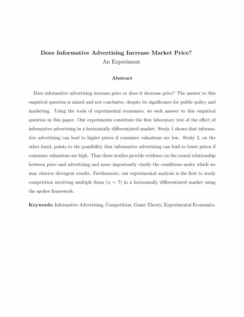
spokes network when N = n = 2. Figure 1 illustrates a market with eight spokes (N = 8)

and seven firms (n = 7). Consumers have the same valuation, v, for all products.

It is assumed that consumers are completely uninformed about a product unless they are

6

Fig. 1. An Illustrative Spokes Model: A market with eight spokes (N = 8) and seven firms(n = 7)

li

exposed to its advertisement. Furthermore, each consumer considers at most two products at

the time of purchase. All consumers consider their local product and it is their first preferred

product. The probability of being informed about it is φ. The second preferred product in

the consideration set is one of the nonlocal products of which the consumer is informed.

Thus the composition of the consideration set is endogenous to the model. The assumption

that consumers prefer at most two products helps to obtain pure strategy equilibrium and

is consistent with the notion that consumers have finite consideration set (Nedungadi 1990).

Now we outline the approach to deriving the demand for firm j’s product for any given price

profile (p1, p2, . . . , pn), relegating the detailed derivation to the appendix. Note that Firm j’s

product could be the first preferred (local) product or the second preferred (nonlocal) product

in a consumer’s consideration set, and that consumers could be informed or uniformed about

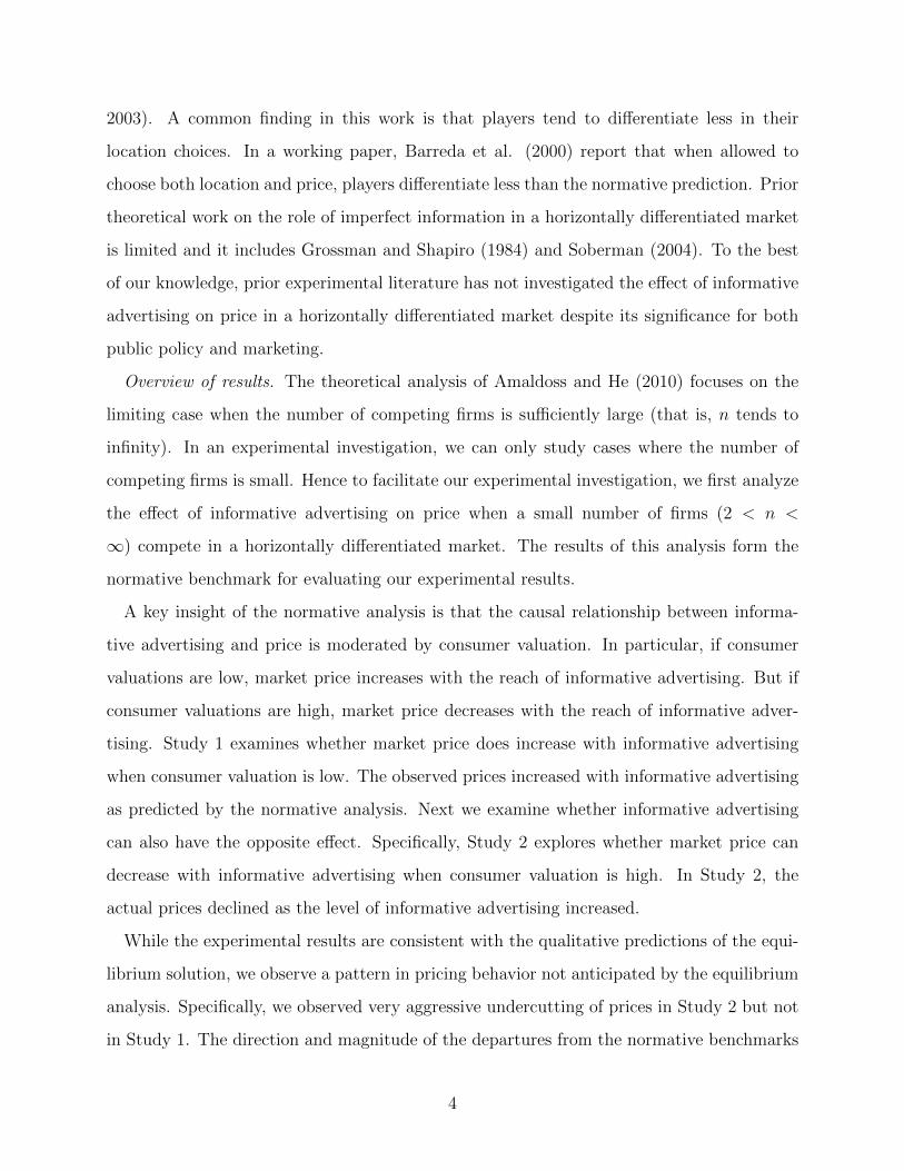
it. Hence, we can partition consumers who purchase product j into four segments as shown

in Figure 2. In Segment 1, Firm j’s product is the first preferred product in the consideration

7

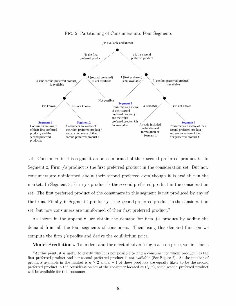
Fig. 2. Partitioning of Consumers into Four Segments

j is available and known

j is the first preferred product

j is the second preferred product

k (the second preferred product) is available

k (second preferred)is not available

k (first preferred)is not available k (the first preferred product)

is available

k is known k is not known

Segment 1Consumers are awareof their first preferred product j and the second preferred product k

Already included in the demand formulation of

Segment 1

Not possible

Segment 2Consumers are aware of their first preferred product jand are not aware of their second preferred product k

Segment 3Consumers are awareof their second preferred product jand their first preferred product k is not available

Segment 4Consumers are aware of their second preferred product jand are not aware of their first preferred product k

k is not knownk is known

set. Consumers in this segment are also informed of their second preferred product k. In

Segment 2, Firm j’s product is the first preferred product in the consideration set. But now

consumers are uninformed about their second preferred even though it is available in the

market. In Segment 3, Firm j’s product is the second preferred product in the consideration

set. The first preferred product of the consumers in this segment is not produced by any of

the firms. Finally, in Segment 4 product j is the second preferred product in the consideration

set, but now consumers are uninformed of their first preferred product.2

As shown in the appendix, we obtain the demand for firm j’s product by adding the

demand from all the four segments of consumers. Then using this demand function we

compute the firm j’s profits and derive the equilibrium price.

Model Predictions. To understand the effect of advertising reach on price, we first focus

2At this point, it is useful to clarify why it is not possible to find a consumer for whom product j is thefirst preferred product and her second preferred product is not available (See Figure 2). As the number ofproducts available in the market is n ≥ 2 and n − 1 of these products are equally likely to be the secondpreferred product in the consideration set of the consumer located at (lj , x), some second preferred productwill be available for this consumer.

8

on the case where consumer valuation is low. Specifically, we consider the case where for

some consumers the valuation is lower than the traveling cost and the purchase price of the

second preferred product, that is 12<

v−pjt

< 1. These consumers can still purchase their

first preferred product. On examining the equilibrium price corresponding to this case, we

have the following prediction.

Prediction 1 When consumer valuations are low, equilibrium price can increase with ad-

vertising reach.

We prove this claim in the Appendix. The intuition for Prediction 1 is as follows. As

consumers become better informed, some consumer segments expand while others contract.

Specifically, the proportion of consumers whose first and second preferred products are both

available (Segment 1) and consumers whose first preferred product is non-existent (Segment

3) increases in size, while the proportion of consumers who are unaware of the existence of

their first or second preferred product (Segment 2 and Segment 4) declines in size. Further-

more, being better informed helps consumers to find their desired product variety and gives

firms an opportunity to charge a higher price (anti-competitive effect). At the same time,

informative advertising also makes consumers more aware of competing product alternatives

and thereby increase price competition (pro-competitive effect). The anti-competitive effect

dominates when consumer valuation is low. Put differently, although a higher advertising

reach increases the proportion of consumers who are aware of both of their preferred prod-

ucts, price elasticity can decrease. This is because when valuation is low, some consumers

do not find it worthwhile to engage in comparison shopping regardless of awareness. Con-

sequently, the substitutability between the first and second preferred products is lower. In

this context, higher advertising reach increases the proportion of consumers who are aware

of one of their preferred products only. Hence, when consumer valuations are low, higher

advertising reach reduces price elasticity. For an example, consider the case when advertis-

ing reach is low with φ = 0.1, v = $1.2, N = 8, n = 7, t = 1, α = $0.1. In this case, the

symmetric pure strategy equilibrium price is 39.12 cents. Now if advertising reach rises to

φ = 0.5, the equilibrium price increases to 45.82 cents. The proof for this claim can be seen

in the Appendix (Claim 1). Next we explore whether this finding can be reversed.

9

When consumer valuation is high, all consumers gain a surplus by buying any product

in their consideration set implying that valuation is more than the traveling cost and the

purchase price of even the second preferred product, that isv−pjt≥ 1. On analyzing the

equilibrium price for this case, we have the following prediction.

Prediction 2 When consumer valuations are sufficiently high, price decreases with adver-

tising reach.

As discussed earlier, informative advertising creates both an anti-competitive effect and a

pro-competitive effect. Together, Prediction 1 and Prediction 2 clarify that the net influence

of these two forces is moderated by consumer valuation. In particular, when consumer

valuation is high the marginal consumer is willing to consider all the product alternatives

she is aware of and this strengthens the pro-competitive effect. That is, when consumer

valuation is sufficiently high, a higher level advertising reach increases the substitutability

between the first and second preferred products, raises price elasticity and lowers prices. For

an illustration of the equilibrium prediction, consider the low φ condition where φ = 0.2,

v = $10, N = 8, n = 7, and α = $1. In equilibrium, price should be 61.20 dimes in

this condition. Now if we increase advertising reach to φ = 0.5 keeping all other variables

constant, the equilibrium price reduces to 23.04 dimes. The proof for this claim is presented

in the Appendix (Claim 2). Next, we proceed to subject these theoretical predictions to an

experimental test.

STUDY 1

The purpose of Study 1 is to assess whether price increases with informative advertising

when consumer valuations are low (Proposition 1). To make causal inference about the

relationship between advertising level and price, we need to exogenously vary the level of

advertising and study its effect on observed price. Furthermore, we need to randomly assign

firms to the different levels of advertising so that all other variables are kept constant. We

exercise this level of control in our experiment. The experimental results provide evidence

that informative advertising can increase price. On further comparing the observed prices

10

against the normative benchmarks, we notice small but significant departures from the equi-

librium predictions. Although the equilibrium solution is the same for all players, we observe

heterogeneity in the behavior of individual participants. We also see trends in the prices over

the several iterations of the game raising the possibility that our participants might have

engaged in adaptive learning. Next we outline the experimental design and then discuss this

findings.

Experimental Design. Treating the level of advertising reach as a between-participant

variable, we ran two groups where the level of advertising reach was low (φ = 0.1) and

another two groups where it was high (φ = 0.5). The other variables of the model were held

constant in all the four groups: N = 8, n = 7, t = 1, v = $1.2, and α = $0.1. We chose this

set of parameters because it leads to a significant rise in equilibrium price if advertising reach

increases from 0.1 to 0.5 (as shown in the previous section). Each group was comprised of

fourteen participants. In each trial, the fourteen participants were randomly divided into two

oligopolies of seven participants. By varying the composition of each oligopoly from trial to

trial and not revealing the identity of the players, we obtained data on multiple replications

of our game (see also Carare, Haruvy and Prasad 2007, Amaldoss and Jain 2005).

Procedure. We invited graduate and undergraduate students to participate in a decision

making study promising them a show-up fee and additional monetary reward contingent on

their performance. On average, participants earned $28.47. As the focus of our experimental

investigation is on the pricing behavior of firms, we abstract away from the demand side of

the market by using the aggregate demand function derived from our consumer model (see

Selten and Apesteguia 2005 for a similar design). Hence, participants played the role of

firms, while the computer played the role of consumers. The detailed instructions provided

to participants can be seen in the Appendix.

Although computer played the role of consumers as per the demand function, we still

provided participants a verbal description of the market. The market was described as a

town with eight streets emanating from the center of the town. At the end of seven of

these streets there is a store, but there is no store in one of the streets. All the stores offer

products of the same quality level. Each street is half a unit long with an equal number

11

of consumers residing in each street. Furthermore, consumers are spread uniformly along

each street. Consumers in each street prefer the product that is available in their local

store. In addition to this product, their consideration set may include another product from

the set of products whose advertisements they have seen. In the low φ treatment, there

is a 10% chance that consumers are aware of the advertisement of a store, whereas in the

high φ treatment the probability of consumers being aware of a store’s product is 50%. It

costs money for consumer to travel from their house to a store. It costs less to travel to a

store if the consumer resides in the same street where the store is located, but more if the

consumer has to travel to another street to purchase its product. The travel cost is equal

to the distance traveled. The total cost of purchasing a product thus includes the price of

the product and the travel cost. Now depending on the total cost of purchasing each of the

products in her consideration set, a consumer first decides whether or not to purchase any

product. If she decides to buy, then she selects the store from which to buy its product.

Note that we can project the demand for a given store’s product if we know the focal

firm’s price and the expected average price of all other competing firms (see Equation (A–14)

in the Appendix). We used this simplification to help our participants appreciate the profit

implications of their price and the likely average price of their competitors. At the beginning

of each trial, each participant was asked to indicate her product’s price and the likely average

price of all the other products in the market. The prices were expressed in cents. Based

on these two inputs, the likely profits of the participant were computed using the simplified

demand formulation. After viewing the likely profits, the participant could revise her price

as well as the expected average price of her competitors. It was clarified to each participant

that her competitors might not behave as predicted by her. Furthermore, her actual earnings

only depended on the actual prices charged by her competitors, not her expected average

price. That is, a participant’s likely profits would be close to her actual profits only to

the extent her expectation about competitors’ average price was accurate. The calculator

thus served as a mere computational tool without providing any guidance on normative

behavior. By providing this calculator, we are able to rule out poor computational skills as

a potential explanation for our results. Perhaps, seeing the likely profit impact of a pricing

12

decision (conditional on their belief about competitors’ actions) might help our participants

to think more about how to improve their profits. Furthermore, as noted earlier, it helps us

to focus our investigation on the supply side while abstracting away from the demand side

of the market (Selten and Apesteguia 2005). After all the players confirmed their prices,

the computer displayed the results of the trial: own prices, own profits, average price of

competitors, average profits of competitors.

To familiarize participants with the structure of the game, they were asked to play three

practice trials for which they were not compensated. If they had any questions about the

instructions, the supervisor answered them. After all the participants became familiar with

the structure of the game, they played thirty five actual trials. Participants played the game

anonymously in the sense that neither their identity nor the identities of the competing

players were revealed. This anonymity, coupled with random assignments of participants to

the two oligopolies of seven firms in each trial, reduced scope for building reputation over

the course of the experiment. The goal of our participants was to maximize their individual

profits over several replications of the game. At the end of the experiment, their cumulative

earnings in the experiment were converted into dollars and paid.3

Results. We begin our analysis of the experimental data by examining the aggregate

behavior of our participants. Later we investigate the variation in the behavior of individual

participants, and analyze the trends in prices over the course of the experiment. The second

row of Table 1 presents the average prices observed in Group 1 and Group 2 corresponding to

each treatment of Study 1 and also compares them to the point predictions of the equilibrium

solution. Below, we report the major results.

Experimental Result 1 On average, the observed prices increased with advertising reach

when consumer valuation was low.

3In our experiment, we did not provide any financial incentive for participants to truthfully reveal theirexpectations. Such an incentive has to be in addition to the profits earned in a trial, and it may add alayer of complexity to an already complicated game and potentially impede comprehension. Thus in ourexperiment, it is quite possible that after gaining experience a participant could enter a random number asher expectation, and yet set her price to maximize actual profits (rather than the expected profits displayedby the calculator). Thus, although the calculator is at the disposal of participants, they can choose not touse it. Thus, we only tracked the actual prices and profits, not the expectations. As we discuss later, we caninfer each participant’s expectations about competitors’ prices from her price.

13

Support: In each of the 35 trials of the experiment, we observed the prices in two oligopolies.

Across the two groups of each treatment, we have accumulated 280 data points (2 oligopolies

× 35 trials × 2 groups × 2 treatments = 280 data points). On analyzing this body of data,

we observe that the average market price increased from 38.592 to 42.681 cents as the reach

of advertising increased from 0.1 to 0.5. We can reject the null hypothesis that these two

prices are the same (t = 25.70, p < 0.0001). A nonparametric analysis based on the Wilcoxon

test also rejects the possibility that all these 280 data points are drawn from the same dis-

tribution (Z = 14.14, p < 0.0001). Instead of focusing on the average price in each duopoly,

if we focus on the average price of each individual participant over the course of thirty five

trials and perform a nonparametric analysis on the resulting 56 data points, we obtain sim-

ilar results. Specifically, we can reject the null hypothesis that the average prices of the 56

participants across the two treatments were drawn from the same distribution (Wilcoxon

Z = 5.82, p < 0.0001). If we conduct repeated measures analysis using the data on price

charged by each individual participant in each trial, we again find that price increased with

advertising reach (F(1,54) = 61.62, p < 0.0001). Next we compare the observed prices against

the point predictions of the equilibrium solution.

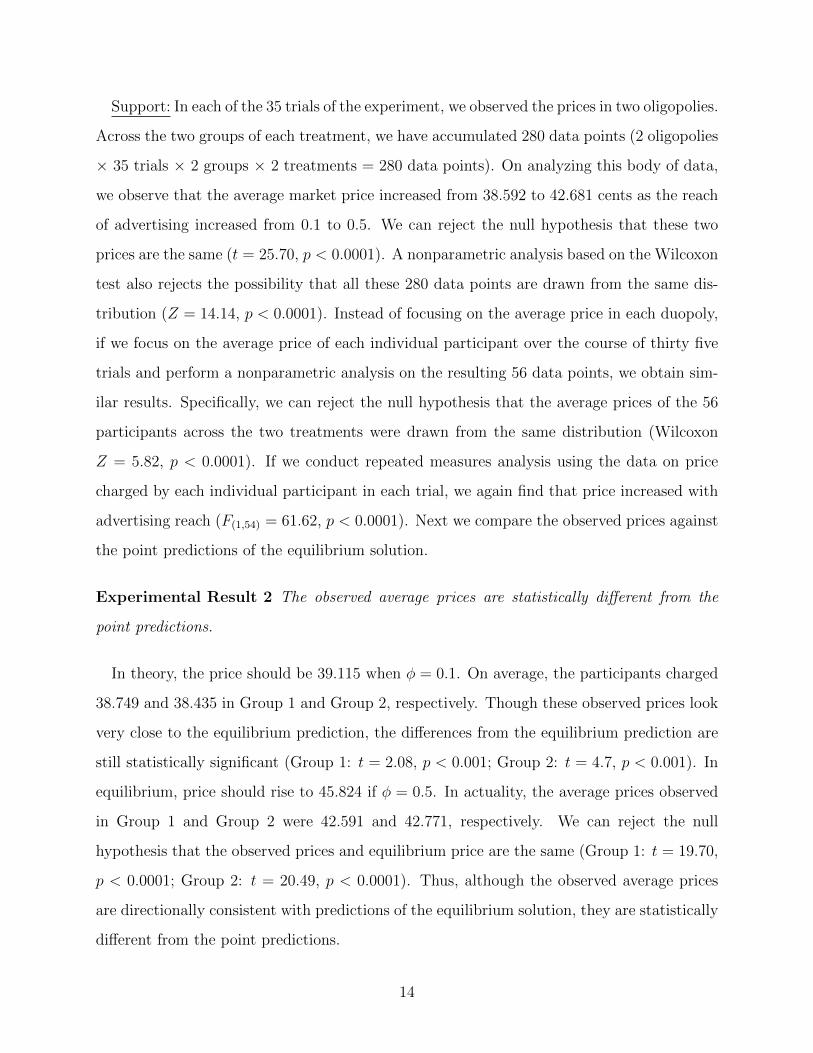
Experimental Result 2 The observed average prices are statistically different from the

point predictions.

In theory, the price should be 39.115 when φ = 0.1. On average, the participants charged

38.749 and 38.435 in Group 1 and Group 2, respectively. Though these observed prices look

very close to the equilibrium prediction, the differences from the equilibrium prediction are

still statistically significant (Group 1: t = 2.08, p < 0.001; Group 2: t = 4.7, p < 0.001). In

equilibrium, price should rise to 45.824 if φ = 0.5. In actuality, the average prices observed

in Group 1 and Group 2 were 42.591 and 42.771, respectively. We can reject the null

hypothesis that the observed prices and equilibrium price are the same (Group 1: t = 19.70,

p < 0.0001; Group 2: t = 20.49, p < 0.0001). Thus, although the observed average prices

are directionally consistent with predictions of the equilibrium solution, they are statistically

different from the point predictions.

14

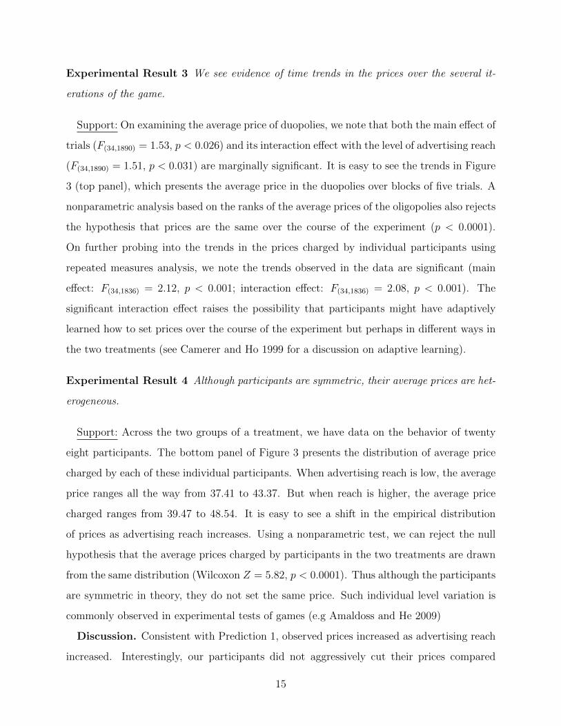
Experimental Result 3 We see evidence of time trends in the prices over the several it-

erations of the game.

Support: On examining the average price of duopolies, we note that both the main effect of

trials (F(34,1890) = 1.53, p < 0.026) and its interaction effect with the level of advertising reach

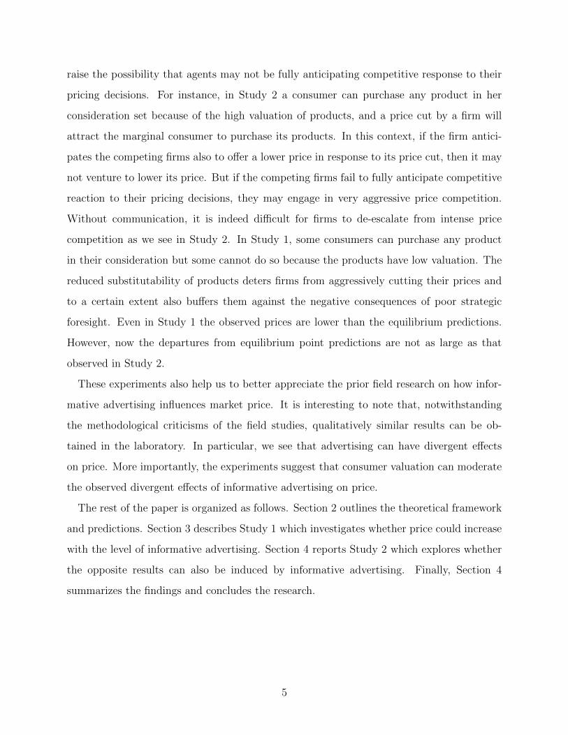
(F(34,1890) = 1.51, p < 0.031) are marginally significant. It is easy to see the trends in Figure

3 (top panel), which presents the average price in the duopolies over blocks of five trials. A

nonparametric analysis based on the ranks of the average prices of the oligopolies also rejects

the hypothesis that prices are the same over the course of the experiment (p < 0.0001).

On further probing into the trends in the prices charged by individual participants using

repeated measures analysis, we note the trends observed in the data are significant (main

effect: F(34,1836) = 2.12, p < 0.001; interaction effect: F(34,1836) = 2.08, p < 0.001). The

significant interaction effect raises the possibility that participants might have adaptively

learned how to set prices over the course of the experiment but perhaps in different ways in

the two treatments (see Camerer and Ho 1999 for a discussion on adaptive learning).

Experimental Result 4 Although participants are symmetric, their average prices are het-

erogeneous.

Support: Across the two groups of a treatment, we have data on the behavior of twenty

eight participants. The bottom panel of Figure 3 presents the distribution of average price

charged by each of these individual participants. When advertising reach is low, the average

price ranges all the way from 37.41 to 43.37. But when reach is higher, the average price

charged ranges from 39.47 to 48.54. It is easy to see a shift in the empirical distribution

of prices as advertising reach increases. Using a nonparametric test, we can reject the null

hypothesis that the average prices charged by participants in the two treatments are drawn

from the same distribution (Wilcoxon Z = 5.82, p < 0.0001). Thus although the participants

are symmetric in theory, they do not set the same price. Such individual level variation is

commonly observed in experimental tests of games (e.g Amaldoss and He 2009)

Discussion. Consistent with Prediction 1, observed prices increased as advertising reach

increased. Interestingly, our participants did not aggressively cut their prices compared

15

to the equilibrium predictions. What can explain this departure from prior experimental

research on competitive games (e.g., Huck 2000)? Note that when consumer valuation is low,

for some consumers the products in their consideration set are substitutable but not so for

others. This substitutability will be further hampered if consumer are not informed of all the

products in the products in their consideration set because of low advertising reach. Hence,

while setting price each participant in Study 1 implicitly weighs the benefits of aggressively

cutting her price to attract some customers away from the competing products (Segment 1)

against the opportunity to charge a higher price to her captive market (Segments 2, 3 and

4). Perhaps the presence of a captive market deterred our participants from charging prices

far lower than the equilibrium prediction.

To further probe into this speculation, we estimated each participant’s belief about oppo-

nents’ average price that is consistent with the best response function and the price charged

by the participant in each trial. On average, the estimated expected price of competitors

was 15.93 and it is much lower that the actually price observed in the low φ treatment.

Similarly, in the high φ treatment the expected price of competitors was 23.35 which is again

lower than the observed price. Thus in Study 1, even though players held very pessimistic

beliefs about competitors prices it was still profitable not to aggressively undercut the price

because of the existence of some consumers in Segments 2, 3 and 4.

As the focus of Prediction 1 is on the effect of advertising reach on price, the analysis and

discussion thus far were centered on prices. In our experiment, we did observe profits. On

average, profits increased as the reach of advertising increased (t = 22.8, p < 0.001). At the

level of individual participants, we see variation in profits, but we can reject the hypothesis

that the average profits of individual participants in the two treatments are drawn from the

same distribution (Wilcoxon Z = 6.41, p < 0.001). Thus, as one may anticipate, the effect

on profits is qualitatively similar to that observed in prices. Having assessed the predictive

accuracy of Prediction 1, we next test Prediction 2.

16

STUDY 2

In Study 2, we seek answer to the question: Is it possible for informative advertising to

cause firms to lower price? According to Prediction 2, the answer is yes. It is useful to

note that this pattern of result is exactly the opposite of the finding reported in Study 1.

In theory, when the valuations are high, consumers could potentially buy either product in

their consideration set. In such a case, when advertising reach increases, the size of the

consumer segment that is aware of both its preferred products grows and the resulting price

competition lowers price. Next we describe experimental procedure and discuss the results

of Study 2.

Experimental Design. Like the previous experiment, Study 2 was designed to focus on

the supply side of the market while abstracting away from the demand side. Consumer valu-

ation was set at v = 10 so that a consumer could purchase any product in her consideration

set. Using a between-participants design, we ran two groups where the level of advertising

reach was low (φ = 0.2) and another two groups where it was high (φ = 0.5). In all these

groups we kept the other model parameters constant, namely N = 8, n = 7, and α = 1.

Each group was comprised of fourteen participants and they were randomly divided in each

trial into two oligopolies of seven participants. The experimental sessions lasted for 35 trials,

excluding three practice trials.

Procedure. We recruited a fresh set of 56 participants for this study and they were

compensated as in the previous study. On average, the participants in this study earned

$28.95. The experimental protocol was similar to the previous study except that we now

used a different set of model parameters.

As in the previous study, in each trial each participant was asked to indicate her product’s

price and the likely average price of all the competitors in the market. The prices were

expressed in dimes. Based on these two prices and the simplified demand function, the

computer displayed the expected profits. The derivation of the simplified demand function

is presented in the Appendix. It was highlighted to each participant that her competitors

might not behave as predicted by her. Further, a participant’s expected profits would be

17

close to actual profits only to the extent her expectation about competitors’ average price

was accurate. Without providing any guidance on equilibrium behavior, the calculator thus

helped our participants to avoid computational error and better understand the likely profit

impact of their decisions. After all the players confirmed their decisions, the results of the

trial were announced and the experiment progressed to the next trial. At the end of 35 trials,

the participants were paid according to their cumulative earnings, debriefed and dismissed.

Results. Table 1 presents the average prices observed in Group 1 and Group 2 for the

two levels of reach and the corresponding equilibrium predictions (see third row). Next we

discuss the major experimental findings.

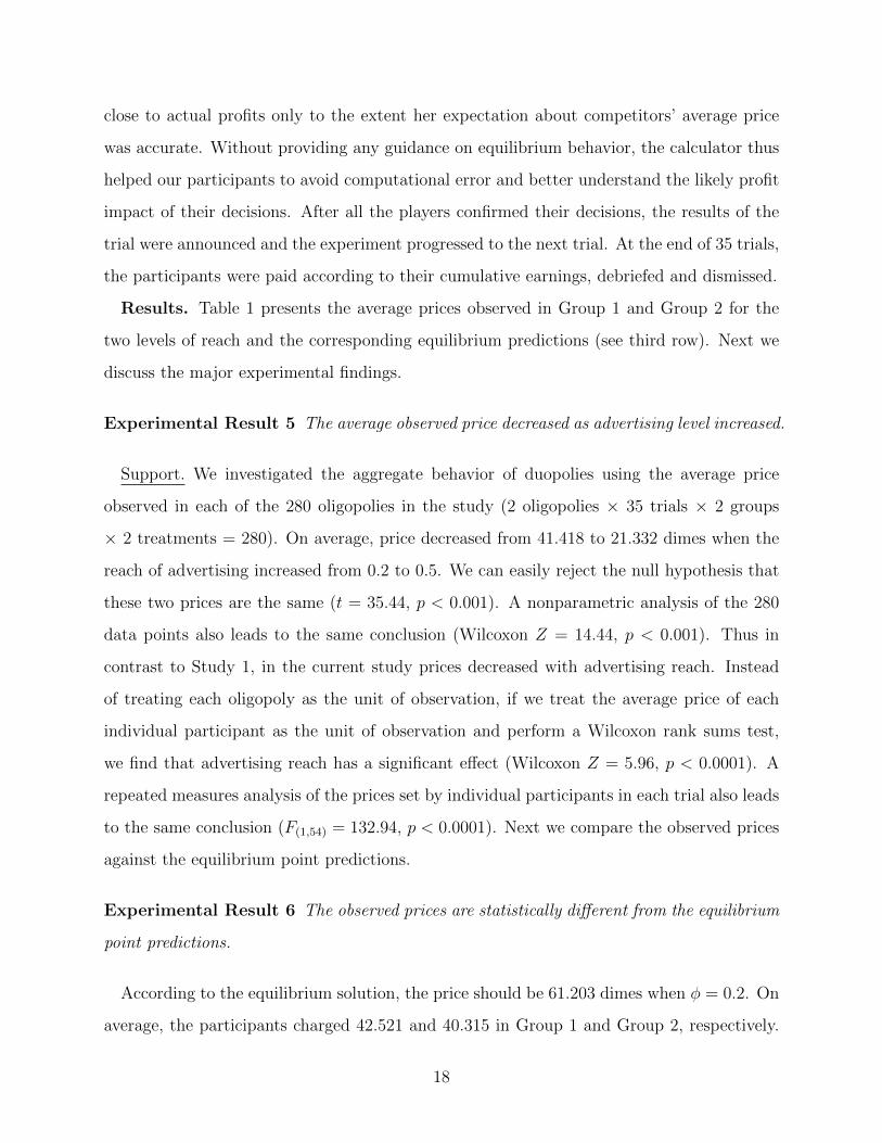
Experimental Result 5 The average observed price decreased as advertising level increased.

Support. We investigated the aggregate behavior of duopolies using the average price

observed in each of the 280 oligopolies in the study (2 oligopolies × 35 trials × 2 groups

× 2 treatments = 280). On average, price decreased from 41.418 to 21.332 dimes when the

reach of advertising increased from 0.2 to 0.5. We can easily reject the null hypothesis that

these two prices are the same (t = 35.44, p < 0.001). A nonparametric analysis of the 280

data points also leads to the same conclusion (Wilcoxon Z = 14.44, p < 0.001). Thus in

contrast to Study 1, in the current study prices decreased with advertising reach. Instead

of treating each oligopoly as the unit of observation, if we treat the average price of each

individual participant as the unit of observation and perform a Wilcoxon rank sums test,

we find that advertising reach has a significant effect (Wilcoxon Z = 5.96, p < 0.0001). A

repeated measures analysis of the prices set by individual participants in each trial also leads

to the same conclusion (F(1,54) = 132.94, p < 0.0001). Next we compare the observed prices

against the equilibrium point predictions.

Experimental Result 6 The observed prices are statistically different from the equilibrium

point predictions.

According to the equilibrium solution, the price should be 61.203 dimes when φ = 0.2. On

average, the participants charged 42.521 and 40.315 in Group 1 and Group 2, respectively.

18

These observed prices are substantially lower than the predicted prices (Group 1: t = 46.69,

p < 0.001; Group 2: t = 41.42, p < 0.001). If φ = 0.5, the equilibrium price should

decline to 23.039 dimes. In actuality, the average prices of Group 1 and Group 2 were

22.877 and 19.788, respectively. We can reject the null hypothesis that the observed prices

and equilibrium prices are the same in Group 2, but not in Group 1 (Group 1: t = 0.22,

p > 0.80; Group 2: t = 6.62, p < 0.001). Now we proceed to examine whether there were

any trends in the prices set by our participants over the course of the experiment.

Experimental Result 7 In Study 2, we see significant trends in prices

Support. The average price in the oligopolies varied over the trials of the experiment but

in different ways in the two treatments (main effect of trials: F(34,1890) = 4.30, p < 0.001;

interaction effect with ad reach:F(34,1890) = 2.03, p < 0.001 ). We obtain similar results if

we conduct a repeated measures analysis using the data on the prices charged by individual

participants in each trial (main effect of trials: F(34,1836) = 7.65, p < 0.001; interaction

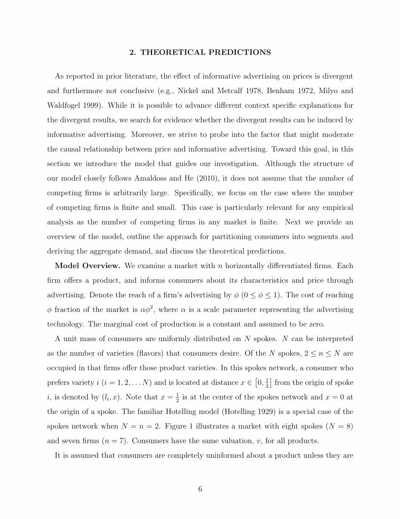
effect:F(34,1836) = 3.62, p < 0.001). The top panel of Figure 4 presents the trends in the

average prices over seven blocks of five trials each. On studying further the behavior of

individual participants, we have the following result.

Experimental Result 8 Although our participants are symmetric, the average price charged

by individual participants are heterogeneous.

Support. The bottom panel of Figure 4 presents the distribution of average prices charged

by each of the twenty eight participants in the two treatments. When advertising reach is

low, the average price charged extends from 28.94 to 55.54. But when reach is higher, the

average price ranges from 17.18 to 55.91. In Figure 4, it is easier to see a leftward shift

in the empirical distribution of prices as advertising reach increased (Wilcoxon Z = 5.96,

p < 0.0001).

Discussion. In contrast to Study 1, prices decreased in the current study when advertising

reach increased. Furthermore, we see very large departures from the point predictions in

Study 2, suggesting that our participants aggressively cut their prices in the latter study. To

19

understand the behavioral basis for this outcome, note that a consumer can gain a surplus

by buying any product in her consideration set as now the valuations are high enough.

Consequently, the products in a consumer’s consideration set are substitutable and hence

a firm can gain share from all its competitors by lowering its price. Furthermore, if the

participant fails to see that its competitors can also cut their prices, then it may trigger

intense price competition. In the absence of any communication among our participants, it

becomes difficult to de-escalate such aggressive behavior and consequently we observe prices

that are far lower than the equilibrium predictions. Our Study 2 results are consistent with

the overreaction to competition seen in Huck et al. (2000).4

As in the previous study, we also estimated the average price that each participant ex-

pected her competitors to charge in a given trial. In the low φ treatment, we find that

the expected average price of competitors was 21.632. Despite such pessimistic views of

their competitors’ prices, participants still charged on average 41.418. This is because, even

though the valuation is high enough that consumers could buy either product in their con-

sideration set, all consumers may not be aware of both the products in their consideration

set because of the low and this makes it less profitable to aggressively cut prices. But when

the reach of advertising grows larger this deterrent effect should weaken. Indeed, in the high

φ treatment, the expected average price of competitors was 19.625 and the price charged

by participants was 21.332. Thus in the high φ treatment the deterrent effect was almost

negligible. This additional analysis helps us to understand how participant’s belief’s come

to influence the market price.

For completeness, we briefly outline the profits observed in Study 2. On average, the

profits decreased when the reach of advertising increased (t = 14.53, p < 0.001). Although

we observe heterogeneity in the average profits of individuals participants, we can easily

reject the hypothesis that the profits in the two treatments are from the same distribution

4For example, in their experiment the observed prices were on average 52.17 though the equilibriumprediction was 76.5 (see p. 47). Their experiments studied oligopolies of three, four or five players; andin general cooperative plays decreased as the number of competitors increased. In our games, as there areseven players in each oligopoly, it reduces further the likelihood of cooperation. While Huck et al. 1999 and2000 test the predictions of Cournot and Bertrand competition using an aggregate demand formulation, weexamine price competition in a horizontally differentiated market.

20

(Wilcoxon Z = 6.41, p < 0.001). As in the previous study, the effect on profits is qualitatively

similar to that observed in prices. Next we test the effect of diverse consumers’ taste on

market price.

In sum, Study 1 and Study 2 show that the effect of advertising on price could vary

with consumer valuation of goods. As noted earlier, in Benham’s natural experiment the

prices of eyeglasses were found to be substantially lower in states that permitted advertising

compared to states that prohibited restrictions. As eyeglasses improve vision as well as how

one looks, consumers are likely to place a high value on eyeglasses (Blumenthal 1983). If

they did so, then Benham’s empirical findings are directionally consistent with Prediction

2. Also consistent with Prediction 1, heavily advertised low valuation goods like cornflakes

are priced higher (Nickell and Metcalf 1978; see also Farris and Reibstein 1979). As we can

only speculate about the valuations of goods covered in these empirical studies, any claim

of even correlational support is open for debate. These prior studies are also vulnerable

to other standard criticisms of cross-sectional analysis. Our laboratory experiment, on the

other hand, is a direct test of the theoretical predictions, and the results are directionally

consistent with the equilibrium solution.

4. CONCLUSIONS

Prior empirical research reports divergent results on the effects of advertising on price. For

example, heavily advertised breakfast cereals were high priced (Nickell and Metcalf 1978; see

also Farris and Reibstein 1979, and Boulding et al. 1994), but prices of eyeglasses declined

with advertising (Benham 1972). A potential way to resolve such divergent findings is to

conduct new field experiments (e.g. Wang and Krishna 2006, Tucker and Zhang 2009), take

advantage of natural experiments (e.g., Milyo and Waldfogel 1999) or use more sophisti-

cated estimation methods (e.g., Ackerberg 2003). Alternatively, one can conduct a tightly

controlled laboratory experiment which is grounded in a game-theoretic model. We pursued

the latter path in the current paper.

Study 1 shows that if consumer valuations are low then market price increases with the

reach of informative advertising. On the contrary, Study 2 establishes that if consumer

21

valuations are high, price declines with advertising. We obtain this result because when

valuation is low the products in a consumer’s consideration set are less substitutable. Fur-

thermore, price sensitivity varies across the different segments of consumers that contribute

to a firm’s demand. Furthermore, when consumer valuation is low, informative advertising

increases the relative importance of consumers who are less sensitive to price, and thereby

motivates firms to charge a higher price. But when consumer valuation is sufficiently high,

all informed consumers obtain a surplus by purchasing any product in their consideration

set. This induces firms to attract the marginal consumer by cutting their prices and conse-

quently market price declines. These experimental findings are reassuring in an important

way: Notwithstanding the methodological criticisms of prior empirical findings on the effects

of advertising, qualitatively similar results can be obtained in the laboratory. Furthermore,

our experiments demonstrate that consumer valuation can moderate the effect of informative

advertising on price.

Our experiments also offer an insight into when we may observe very aggressive under-

cutting of price. The observed prices are close to the equilibrium predictions in Study 1,

but not in Study 2. Why do we observe such a pattern of results? Note that while setting

price, each firm in Study 1 implicitly weighs the prospect of cutting its price (and attracting

some customers away from its competitor) against the benefit of charging a higher price to

her captive market and forgoing some of the competitive market. In this situation, if prod-

ucts are less substitutable because of low valuation or low advertising reach, it deters firms

from engaging in aggressive undercutting of prices. If this deterrent force weakens, we may

observe a downward spiral in prices. In the absence of communication, it is difficult for an

individual firm in an oligopoly to unilaterally extricate itself from aggressive undercutting

of prices. Interestingly, our participants’ beliefs about competitors’ prices are even harsher

than the market reality. Consequently in Study 2 we observe substantial departures from

the equilibrium price.

In several product categories consumers’ taste are very diverse and firms also offer a wide

variety of products. This raises an interesting empirical question: How does diversity in

consumers’ tastes affect market price? Extant empirical literature is yet to answer this

22

question for an important reason. Although it is easy to measure the variety of products

available in a market, it is difficult to reliably assess the variety of products that consumers

seek in a product category. Consequently, it is an even greater empirical challenge to study

the relationship between diversity in consumers’ tastes and price in markets where consumers

are not fully informed about all the competing products. However, it is possible to use our

experimental protocol to study this phenomenon in the laboratory. This will be a fruitful

avenue for further research.

More broadly, experimental investigations could become a useful complement to the em-

pirical literature on the effects of advertising. While laboratory studies have a high degree of

internal validity, one needs to exercise caution in extrapolating the findings to a field setting.

Cross-sectional field studies, on the other hand, guarantee external validity although it is

more challenging to establish causal relationships with such data. Field experiments can

overcome this issue but such an investigation is often costly and impossible to implement in

some settings. A judicious use of these different methods can augment our understanding of

markets (e.g. Krishna and Unver 2008).

The spokes model used in this paper is a very attractive framework for studying spatial

competition and it has several advantages over the traditional models of horizontal differen-

tiation. In contrast to the circle model (Salop 1979), the spokes model allows products and

firms to be symmetric without the need to change the location of the incumbents when a

new firm enters the market. Furthermore, each firm is in direct competition with all other

products in the market. The market also is not assumed to be fully covered and the extent

of coverage actually depends on the number of competing firms and consumer valuations.

Moreover, as demonstrated in this paper, the spokes model has both descriptive validity and

analytical tractability. These benefits should stimulate researchers to apply this framework

to study new issues in horizontally differentiated markets with a large number of competing

firms.

23

REFERENCES

[1] Ackerberg, D. 2003. “Advertising, Learning, and Consumer Choice in Experience Good

Markets: An Empirical Examination.” International Economic Review. 44(3) 1007–

1040.

[2] Amaldoss, W. and C. He. 2010. “Product Variety, Informative Advertising and Price Com-

petition.” Journal of Marketing Research. 47(1) 146–156.

[3] Amaldoss W. and C. He. 2009. “Direct-to-Consumer Advertising of Prescription Drugs: A

Strategic Analysis. ” Marketing Science. 28(3) 472–487.

[4] Amaldoss, W. and S. Jain. 2005. “Pricing of Conspicuous Goods: A Competitive Analysis

of Social Effects.” Journal of Marketing Research. 42(1) 30–42.

[5] Anderson, S. P. and A. de Palma. 2006. “Market Performance With Multiproduct Firms.”

Journal of Industrial Economics. 54(1) 95–124.

[6] Benham, L. 1972. “The Effect of Advertising on the Price of Eyeglasses.” Journal of Law

and Economics. 15(2) 337–52.

[7] Blumenthal, D. 1983. “Beauty: Looking Good in Eyeglasses.” New York Times . June 5.

[8] Brown-Kruse, J., M. Cronshaw, and D. Shenk. 1993. “Theory and Experiments on Spatial

Competition.” Economic Enquiry. 31, 139–165.

[9] Brown-Kruse, J., and D. Shenk. 1993. “Location, Cooperation and Communication.” Inter-

national Journal of Industrial Organization. 18, 59–80.

[10] Cady, J. F. 1976. “An Estimate of the Price Effects of Restrictions on Drug Price Advertis-

ing.” Economic Inquiry. 14(4) 493–510.

[11] Camerer, C. and T. H. Ho. “Experience-Weighted Attraction Learning in Normal Form

Games. ” Econometrica 67 837–874.

24

[12] Carare, O., E. Haruvy and A. Prasad. 2007. “Hierarchical thinking and learning in rank

order contests.” Experimental Economics. 10(3) 305–316.

[13] Chen, Y. and M. Riordan. 2007. “Price and Variety in the Spokes Model.” The Economic

Journal. 117(522) 897–921.

[14] Connor, M. and E. Peterson. 1992. “Market-Structure Determinants of National Brand-

Private Label Price Differences of Manufactured Food Products.” The Journal of In-

dustrial Economics. 40(2) 157–171.

[15] Farris, P. W. and D. J. Reibstein. 1979. “How Prices, Ad Expenditures, and Profits are

Linked.” Harvard Business Review. Nov-Dec, 173–184.

[16] Grossman, G. M. and C. Shapiro. 1984. “Informative advertising with differentiated prod-

ucts.” Review of Economic Studies. 51(1) 63–81.

[17] Hotelling, H. 1929. “Stability in Competition.” The Economic Journal. 39(153) 41–57.

[18] Ho, T-H. and J. Zhang (2008). “Designing Pricing Contracts for Boundedly Rational Cus-

tomers: Does the Framing of the Fixed Fee Matter?” Management Science. 54(4) 686–

700.

[19] Huck, S., H. T. Normann and J. Oechssler 1999. “Learning in Cournot Oligopoly – An

Experiment.” Economic Journal. 109(454) C80–C95.

[20] Huck, S., H. T. Normann and J. Oechssler 2000. “Does Information about Competitors’

Actions Increase or Decrease Competition in Experimental Oligopoly Markets?” Inter-

national Journal of I ndustrial Organization. 18(1) 39–57.

[21] Krishna, A. and U. Unver. 2008. “Improving the Efficiency of Course Bidding at Business

Schools: Field and Laboratory Studies.” Marketing Science. 27(2) 262–282.

[22] Krishnamurthi. L. and S. P. Raj. 1985. “The Effect of Advertising on Consumer Price Sen-

sitivity.” Journal of Marketing Research. 22(2) 119–129.

25

[23] Lim, N. and T. H. Ho. 2007. “Designing Price Contracts for Boundedly Rational Customers:

Does the Number of Blocks Matter? ” Marketing Science. 26(3) 312–326.

[24] Milyo, J. and J. Waldfogel. 1999. “The effect of price advertising on prices: Evidence in the

wake of 44 Liquormart.” The American Economic Review. 89(5) 1081–1096.

[25] Nedungadi, P. 1990. “Recall and Consumer Consideration Sets: Influencing Choice without

Altering Brand Evaluations.” Journal of Consumer Research. 17(Dec) 263–276.

[26] Nickell, S. and D. Metcalf. 1978. “Monopolistic industries and monopoly profits or, are

Kellogg’s cornflakes overpriced?” The Economic Journal. 88(350) 254–268.

[27] Selten, R. and J. Apesteguia 2005. “Experimentally Observed Imitation and Cooperation in

Price Competition on the Circle.” Games and Economic Behavior. 51(1) 171–192.

[28] Salop, S. 1979. “Monopolistic competition with outside goods.” Bell Journal of Economics.

10(1) 141–156.

[29] Soberman, D. 2004. “Research Note: Additional Learning and Implications on the Role of

Informative Advertising.” Management Science. 50(12) 1744–1750.

[30] Tucker, C. and J. Zhang (2009). ”Growing Two Sided Networks by Advertising the User

Base: A Field Experiment.” Marketing Science. Forthcoming.

[31] Wang, Y. and A. Krishna. 2006. “Time-Share Allocations: Theory and Experiment. ” Man-

agement Science. 52(8) 1223–1238.

26

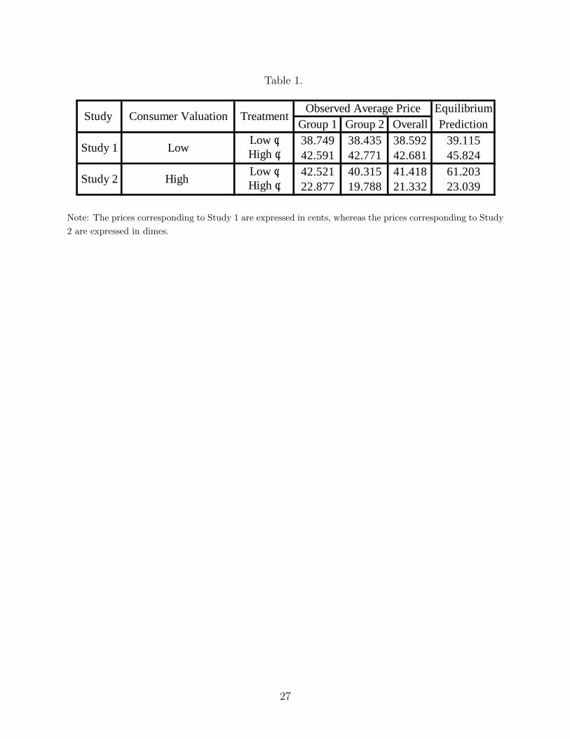
Table 1.

EquilibriumGroup 1 Group 2 Overall Prediction

Low φ 38.749 38.435 38.592 39.115High φ 42.591 42.771 42.681 45.824Low φ 42.521 40.315 41.418 61.203High φ 22.877 19.788 21.332 23.039

Study 2 High

Observed Average PriceStudy Consumer Valuation Treatment

Study 1 Low

Note: The prices corresponding to Study 1 are expressed in cents, whereas the prices corresponding to Study

2 are expressed in dimes.

27

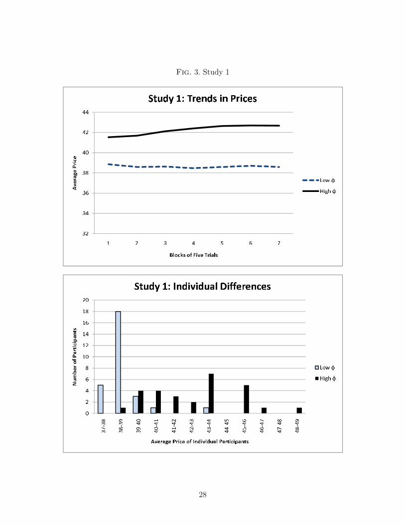
Fig. 3. Study 1

0246810121416182037-38 38-39 39-40 40-41 41-42 42-43 43-44 44-45 45-46 46-47 47-48 48-49Number of Participants Average Price of Individual Participants

Study 1: Individual Differences Low φHigh φ32343638404244

1 2 3 4 5 6 7Average Price Blocks of Five TrialsStudy 1: Trends in Prices Low φHigh φ

28

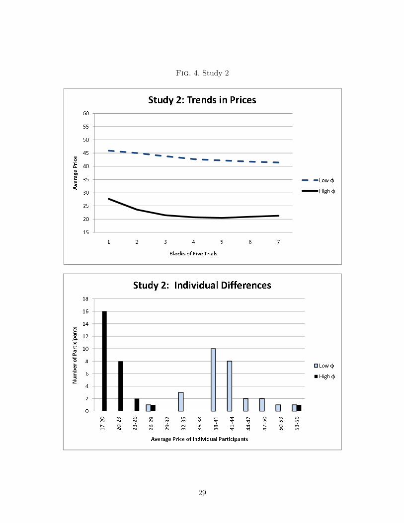
Fig. 4. Study 2

02468101214161817-20 20-23 23-26 26-29 29-32 32-35 35-38 38-41 41-44 44-47 47-50 50-53 53-56Number of Participants Average Price of Individual Participants

Study 2: Individual Differences Low φHigh φ15202530354045505560

1 2 3 4 5 6 7Average Price Blocks of Five TrialsStudy 2: Trends in Prices Low φHigh φ

29

APPENDIX

In this appendix, we derive the aggregate demand function and equilibrium price. We then

provide proofs to the theoretical predictions and claims (numerical examples) presented in

the paper. The appendix is organized as follows. We first derive the aggregate demand,

and the equilibrium price for the case where consumer valuations are low (Lemma 1). Next,

we show that price can increase with advertising reach when consumer valuations are low

(Prediction 1). We then derive the equilibrium point predictions for Study 1 (Claim 1).

Turning attention the case where consumer valuations are high, we derive the equilibrium

price (Lemma 2), show that price increases decreases with advertising reach (Prediction 2),

and then derive the equilibrium point predictions for Study 2 (Claim 2).

We derive the demand for firm j, j ∈ {1, . . . , n}, for any given price profile (p1, p2, . . . , pn).

Based on product availability and information (see Figure 2 on page 8), we can classify

consumers into four relevant segments as we described below. To eliminate the trivial cases,

we assumev−pjt

> 12

and|pk−pj |

t≤ 1.

Segment 1. Firm j’s product is the local product and hence the first preferred product

in the consideration set of a consumer in this group. The probability that a consumer is

aware of her first preferred product j is φ. Any nonlocal product about which the consumer

is informed could be the second preferred product in her consideration set. Thus the second

preferred product in the consideration set, namely k 6= j where k ∈ {1, . . . , n}, is drawn from

the set of products to which an individual consumer has been exposed through advertising.

The joint probability that the consideration set of a consumer located on spoke lj includes

products j and k is given by 1n−1φ

[1−

(1− φ̂

)n−1].5 The density of such consumers is 2

N,

and the demand from this group of consumers is given by:

2

N

1

n− 1φ

[1−

(1− φ̂

)n−1] ∑k 6=j,k∈{1,...,n}

(1

2+pk − pj

2t

). (A–1)

Segment 2. Firm j’s product is the first preferred product in the consideration set of

a consumer in this group also. However, the consumer is uninformed about their second

5Please see Amaldoss and He (2010) for a proof.

30

preferred product. In this case the probability that the consumer located on spoke lj only

considers product j is given by φ(

1− φ̂)n−1

. The demand from this group of consumers is

given by1

Nφ(1− φ̂)n−1. (A–2)

Next we turn attention to cases where firm j’s product is the second preferred product

in the consideration sets of consumers. As the number of products available in the market

is n ≥ 2 and n − 1 of these products are equally likely to be the second preferred product

in the consideration set of the consumer located at (lj, x), some second preferred product

will always be available for the consumer at (lj, x). However, consumers may be uninformed

about their second preferred products.

Segment 3. The first preferred product (variety) k preferred by consumers in this group is

not produced by any of the n firms, and product j is the second preferred product in their

consideration set. The demand from this group of consumers is given by

2NN−nn

[1− (1− φ)

(1− φ̂

)n−1] (v−pjt− 1

2

)for 1

2<

v−pjt

< 1

1NN−nn

[1− (1− φ)

(1− φ̂

)n−1]for

v−pjt≥ 1

(A–3)

The region 12<

v−pjt

< 1 corresponds to the situation where consumers always derive positive

surplus from purchasing their first preferred product but the valuation is not high enough for

some consumers to obtain positive surplus from purchasing their second preferred product.

By contrast, whenv−pjt≥ 1, consumers derive positive surplus from purchasing both their

first and second preferred products.

Segment 4. Consumers in this segment are uninformed of their first preferred product and

product j is the second preferred product in their consideration set. The demand from this

group of consumers is given by

2N

1−φ̂n−1

[1− (1− φ)

(1− φ̂

)n−2] ∑k 6=j,k∈{1,...,n}

(v−pjt− 1

2

)for 1

2<

v−pjt

< 1

2N

1−φ̂n−1

[1− (1− φ)

(1− φ̂

)n−2] ∑k 6=j,k∈{1,...,n}

12

forv−pjt≥ 1

(A–4)

31

When consumer valuations are low (that is, 12<

v−pjt

< 1), the demand function for firm

j’s product is given by

qj =

1Nφ

[1−

(1− φ̂

)n−1](1 + 1

n−1

n∑i=1

pi−pjt

)+ 1

Nφ(1− φ̂)n−1

+ 2N

N−nn

[1− (1− φ)

(1− φ̂

)n−1]+(

1− φ̂)[

1− (1− φ)(

1− φ̂)n−2]

(v−pj

t− 1

2

) (A–5)

We assume that firms set their prices simultaneously and focus on symmetric pure strategy

equilibrium.

When consumer valuations are sufficiently high (i.e.,v−pjt≥ 1), the demand function for

firm j’s product is given by

qj =

1Nφ

[1−

(1− φ̂

)n−1](1 + 1

n−1

n∑i=1

pi−pjt

)+ 1

Nφ(

1− φ̂)n−1

+ 1N

N−nn

[1− (1− φ)

(1− φ̂

)n−1]+(

1− φ̂)[

1− (1− φ)(

1− φ̂)n−2]

(A–6)

Lemma 1 When 12<

v−pjt

< 1, the equilibrium price is

p∗j =N (2v − t) [1− (1− φ)n]− 2nφ (v − t)

4N [1− (1− φ)n]− nφ (1− φ)n−1 − 3nφ. (A–7)

Proof. Using the demand function given in Equation (A–5) and the cost functionA (φ;α) =

αφ2, we obtain the following profits for firm j:

πj = pj

1Nφ

[1−

(1− φ̂

)n−1](1 + 1

n−1

n∑i=1

pi−pjt

)+ 1

Nφ(1− φ̂)n−1

+ 2N

N−nn

[1− (1− φ)

(1− φ̂

)n−1]+(

1− φ̂)[

1− (1− φ)(

1− φ̂)n−2]

(v−pj

t− 1

2

)− αφ2 (A–8)

Using the first-order condition∂πj

∂pj= 0 and noting that in the symmetric pure strategy

equilibrium, p∗j = p∗k and φ = φ̂, we solve for the optimal price and find that p∗j is as given

32

in Equation (A–7).

Prediction 1 When consumer valuations are low, (that is, 12<

v−pjt

< 1), equilibrium

price can increase with advertising reach.

Proof. When consumer valuations are low, the equilibrium price is given by Equation

(A–7). It follows that

∂p∗

∂φ= − n

(1− φ)2{

4N [1− (1− φ)n]− 3nφ− nφ (1− φ)n−1}2 ·

N (1− φ)2 (2v − 5t) +N (1− φ)2n (2v − t)

+ (1− φ)n

2N ((3t− 2v) + φ (2nt+ 2v − 5t))

−φ2 (n− 1) (5Nt− 2nt− 2v (N − n))

(A–9)

The case when N = 8 and n = 7 forms the basis for the experimental investigations presented

in the paper. For this case, we have:

limφ→0

∂p∗

∂φ= −(21v − 33t)

196> 0 for v ≤ 33

21t

limφ→1

∂p∗

∂φ= −(112v − 280t)

121> 0 (A–10)

Similarly, we can establish the comparative statics for any given n and N . For a more

general proof, readers are referred to Amaldoss and He (2010).

Claim 1 When v = $1.2, N = 8, n = 7, t = 1, α = $0.1, the symmetric pure strategy

equilibrium price is 39.12 cents if φ = 0.1. The equilibrium price increases to 45.82 cents

when advertising reach rises to φ = 0.5.

On substituting v = $1.2, N = 8, n = 7, t = 1, α = $0.1, and φ = 0.1 into Equation

(A–7), we have p∗j = 39.12 cents. The equilibrium price increases further to 45.82 cents when

advertising reach rises to φ = 0.5.

Note that in equilibrium when φ = 0.1, we havev−pjt

= 0.809; and similarly when φ = 0.5

we obtainv−pjt

= 0.742. Thus in both treatments 12<

v−pjt

< 1.

33

Lemma 2 Whenv−pjt≥ 1, the equilibrium price is

p∗j =Nt (1− φ)

nφ

1− (1− φ)n

1− φ− (1− φ)n. (A–11)

Proof. On inserting firm j’s demand given in Equation (A–6) and the cost function

A (φ;α) = αφ2 into the profit function, we can express firm j’s profits as:

πj = pj

1Nφ

[1−

(1− φ̂

)n−1](1 + 1

n−1

n∑i=1

pi−pjt

)+ 1

Nφ(

1− φ̂)n−1

+ 1N

N−nn

[1− (1− φ)

(1− φ̂

)n−1]+(

1− φ̂)[

1− (1− φ)(

1− φ̂)n−2]

− αφ2 (A–12)

Solving∂πj

∂pj= 0 and noting that in the symmetric pure strategy equilibrium, p∗j = p∗k and

φ = φ̂, we obtain p∗j as given in Equation (A–11).

Prediction 2 When consumer valuations are sufficiently high (i.e.,v−pjt≥ 1), price

decreases with advertising reach.

Proof. When consumer valuations are high, the equilibrium price is given by Equation

(A–11). Therefore, we obtain:

∂p∗

∂φ=

∂

∂φ

{Nt [1− (1− φ)n]

nφ[1− (1− φ)n−1

]}

= Nt

[2 (1− φ)− (n− 1)φ2 − (1− φ)n

](1− φ)n − (1− φ)2

nφ2 (1− φ)2[1− (1− φ)n−1

]2 (A–13)

Note that the denominator of ∂p∗

∂φis positive for φ ∈ (0, 1). It can be shown that the

numerator is always negative for any φ ∈ (0, 1). Therefore, it follows that ∂p∗

∂φ< 0.

Claim 2 When v = $10, N = 8, n = 7, and α = $1, the symmetric pure strategy equilibrium

price is 61.20 dimes if φ = 0.2. The equilibrium price p∗ reduces to 23.04 dimes when

advertising reach increases to φ = 0.5.

Inserting v = $10, N = 8, n = 7, α = $1, and φ = 0.2 into Equation (A–11), we obtain

p∗j = 61.20 dimes. The equilibrium price p∗j reduces to 23.04 dimes when advertising reach

34

increases to φ = 0.5.

Also in equilibrium,v−pjt

is 3.88 when φ = 0.2, and it becomes 7.7 when φ = 0.5. Thus,

in both treatmentsv−pjt

> 1.

SIMPLIFIED EXPECTED DEMAND

When consumer valuation is low, the demand function given in Equation (A–5) can be

simplified as follows to obtain the expected demand of firm j:

qj =

1Nφ

[1−

(1− φ̂

)n−1](1 +

p−j−pjt

)+ 1

Nφ(1− φ̂)n−1

+ 2N

N−nn

[1− (1− φ)

(1− φ̂

)n−1]+(

1− φ̂)[

1− (1− φ)(

1− φ̂)n−2]

(v−pj

t− 1

2

) (A–14)

Thus, we can project the demand for a given store’s product if we know the focal firm’s

price and the average price of all other competing firms. In our experimental investigation,

we used this simplification to help our participants appreciate the profit implications of their

price and the likely average price of their competitors.

When consumer valuation is high, the demand function given in Equation (A–6) can be

further simplified to obtain the following expected demand of firm j:

qj =

1Nφ

[1−

(1− φ̂

)n−1](1 +

p−j−pjt

)+ 1

Nφ(

1− φ̂)n−1

+ 1N

N−nn

[1− (1− φ)

(1− φ̂

)n−1]+(

1− φ̂)[

1− (1− φ)(

1− φ̂)n−2]

(A–15)

35