IFS Working Paper W19/01 Alex Armand

Alexander Coutts

Pedro C. Vicente

Ines Vilela

Does information break the political resource curse? Experimental evidence from Mozambique

Does Information Break the Political Resource Curse?

Experimental Evidence from Mozambique*

Alex Armand Alexander Coutts Pedro C. Vicente Ines Vilela

January 2019

Abstract

The political resource curse is the idea that natural resources can lead to the deterioration

of public policies through corruption and rent-seeking by those closest to political power. One

prominent consequence is the emergence of conflict. This paper takes this theory to the data

for the case of Mozambique, where a substantial discovery of natural gas recently took place.

Focusing on the anticipation of a resource boom and the behavior of local political structures

and communities, a large-scale field experiment was designed and implemented to follow the

dissemination of information about the newly-discovered resources. Two types of treatments

provided variation in the degree of dissemination: one with information targeting only local

political leaders, the other with information and deliberation activities targeting communities

at large. A wide variety of theory-driven outcomes is measured through surveys, behavioral

activities, lab-in-the-field experiments, and georeferenced administrative data about local con-

flict. Information given only to leaders increases elite capture and rent-seeking, while infor-

mation and deliberation targeted at citizens increases mobilization and accountability-related

outcomes, and decreases violence. While the political resource curse is likely to be in play,

the dissemination of information to communities at large has a countervailing effect.

JEL codes: D72, O13, O55, P16.

Keywords: Natural Resources, Curse, Natural Gas, Information, Deliberation, Rent-seeking,

Mozambique.*Armand: University of Navarra and Institute for Fiscal Studies (e-mail: aarmand@unav.es); Coutts: Nova School

of Business and Economics, Universidade Nova de Lisboa, and NOVAFRICA (e-mail: alexander.coutts@novasbe.pt);Vicente: Nova School of Business and Economics, Universidade Nova de Lisboa, BREAD, and NOVAFRICA (e-mail: pedro.vicente@novasbe.pt); Vilela: Nova School of Business and Economics, Universidade Nova de Lisboa,and NOVAFRICA (e-mail: ines.vilela.2013@novasbe.pt). We would like to thank Laura Abramovsky, Paul Atwell,Jaimie Bleck, Paul Friesen, Macartan Humphreys, Lakshmi Iyer, Patricia Justino, Danila Serra, Michele Valsecchiand seminar/conference participants at IFS-London, IDS-Sussex, IGC, 3ie/AfrEA, Notre Dame, Portsmouth, SouthernMethodist, WZB-Berlin, SEEDEC, Nova-Lisbon, EGAP, NEUDC-Cornell, Bergen and CMI for helpful comments.This project would not be possible without the generous and insightful help of Imamo Mussa. We also acknowledgefruitful collaborations with our institutional partners, which included the Provincial Government of Cabo Delgado. Weare grateful to Henrique Barros, Benedita Carvalho, Ana Costa, Joao Dias, Lucio Raul, Matteo Ruzzante, AlexanderWisse, and a large team of enumerators, who were vital in the successful completion of this project in the field. Ethicsapproval was secured from Universidade Nova de Lisboa. We wish to acknowledge financial support from 3ie Interna-tional Initiative for Impact Evaluation (grant number TW8R2/1008) and the International Growth Centre (grant number89330). Vicente also acknowledges support by the Kellogg Institute at the University of Notre Dame.

1

1 Introduction

Since Adam Smith’s Wealth of Nations, which contains several unfavorable references to mining

activities, economists have been wary of potential problems arising from the exploitation of natural

resources. Gelb (1988) and Auty (1993) were the first to propose the term resource curse after ob-

serving a close relationship between mineral windfalls and the contraction of traded sectors, i.e.,

the Dutch Disease. In the 1990s, African countries such as Nigeria, Angola, and Sierra Leone,

rich in oil and diamonds, became prominent cases for the development of new theories. These

contributed to the argument that the resource curse was also related to political economy mecha-

nisms involving widespread corruption (Treisman, 2000) and civil conflict (Collier and Hoeffler,

2004). While a significant body of research attends this phenomenon, little is known about how

the presence of resources may directly impact the behavior of local political leaders and regular

citizens.

The focus of this paper is on understanding the political roots of the resource curse. Theories

based on political economy mechanisms start by associating the exploitation of natural resources

with movements towards rent-seeking in the economy, at the expense of more productive activi-

ties (Tornell and Lane, 1999; Baland and Francois, 2000; Torvik, 2002). The curse become more

explicitly political with Robinson et al. (2006), who posit that following news of a resource dis-

covery, politicians become more interested in securing political power, pursuing corrupt behaviors

and inefficient policies, and thus imposing negative consequences for the economy. A prominent

symptom of these policies is the emergence of violence and civil conflict. Robinson et al. (2006)

believe the curse is avoidable by promoting institutions that strengthen political accountability.

However, causal evidence regarding the effects of the provision of information in the context of a

future resource boom is scarce.

This paper tests for the presence of the political resource curse by analyzing reactions to news of a

major resource discovery, i.e., the anticipation of a resource windfall. The focus is on first reactions

at the local level, in particular those of citizens and local politicians. A large-scale randomized field

experiment was conducted in 206 communities in Northern Mozambique in 2017, after a massive

discovery of natural gas in the Rovuma basin, Cabo Delgado province. This provides a unique

setting to study the political resource curse since the discovery, labeled the largest worldwide

in many years, has the potential to generate a substantial impact on the Mozambican economy.1

Facing limited media independence and penetration, as well as poor knowledge of the discovery in

the province, a large coalition of governmental and non-governmental organizations, active in the

international, national, and local arenas sponsored the efforts of disseminating information about1See CNN (Is Mozambique the next oil and gas hub?, 03/05/2017) or The Financial Times (Mozambique to become

a gas supplier to world, 27/06/2018) for two recent articles about natural gas in Mozambique.

2

the discovery and management of natural resources at the community level.

In cooperation with these partners, two interventions were designed and implemented. In the first,

only local political leaders received the information module; in the second, it was delivered to both

local leaders and citizens, targeting communities at large. In one version of the latter intervention,

the information module was further accompanied by the organization of citizen deliberation meet-

ings to discuss public policy priorities in relation to the future natural gas windfall. This design

provided the opportunity to test for changes in behavior in a low-accountability context when only

the local political elite is informed, and when the community at large is informed, with potentially

higher levels of accountability. Most importantly for policy, this setting allows testing the role of

information dissemination and of citizen deliberation on avoiding the curse.

The design of the experiment and of the measurements were included in a pre-analysis plan reg-

istered on the American Economic Association RCT registry (Armand et al., 2017), and followed

closely in the analysis. The experimental design incorporates a wide range of measurements,

including baseline and endline surveys, structured community activities (SCAs), lab-in-the-field

experiments, and georeferenced data about violent events. Measurements were compiled specifi-

cally to depict behavioral changes among both local leaders and citizens, consistent with previous

theoretical work on the political resource curse. Some behavioral measurements were originally

developed for this project–namely SCAs measuring favoritism and rent-seeking, as well as a rent-

seeking game; other behavioral measurements follow previous contributions, as in Casey et al.

(2012), Batista and Vicente (2011), and Collier and Vicente (2014).

Outcome measures are grouped in five sets. The first is related to awareness and knowledge re-

garding natural resources, based on survey questions, measured both at baseline and endline, and

administered to both local leaders and citizens. The second set is related to elite capture by local

leaders, centered on behavioral measurements, including SCAs on resources intended for commu-

nity use (e.g., zinc sheets for roof construction, funds for meetings) and on the appointment of a

community taskforce, as well as leader behavior in a trust game. The third set is connected to rent-

seeking by leaders and citizens, relying primarily on an auction eliciting willingness to engage in

rent-seeking, and a novel rent-seeking lab-in-the-field game. The fourth set links to mobilization,

trust, and the demand for political accountability by citizens. The outcomes on mobilization are

grounded in survey-based measures of social capital, an SCA involving a matching grant activ-

ity that includes behavior associated with community meetings, and a public goods game. The

outcomes on trust and accountability are based on survey questions, an SCA involving a postcard

activity measuring demand for accountability, and citizen behavior in a standard trust game. Fi-

nally, the fifth set relates to violence, particularly important given the sudden rise in violent events

attributed to extremist groups recruiting support in the province, which characterized the period at

3

end of the project and starting in October 2017.2 Local conflict is measured through self-reported

violence from surveys and through the incidence of conflict as measured by international event-

based datasets (ACLED and GDELT). Given the large set of outcomes studied, multiple inference

is addressed considering the joint-dependence of outcomes and following step-down multiple hy-

pothesis testing (Romano and Wolf, 2005).

Clear positive effects of community-level information dissemination are observed on awareness

and knowledge about the natural gas discovery among citizens and leaders. In particular, citizens

become more optimistic regarding the future benefits of the discovery for their communities and

households. On the contrary, when only leaders receive information, no change occurs in aware-

ness and knowledge among citizens, while leaders become more acknowledged. In this case, im-

pacts on increased elite capture are identified in terms of leaders’ attitudes in favor of corruption,

misuse of funds for public purposes, and less meritocratic appointments of community members

for public service. Targeting information only at leaders increases by 27 percentage-points the

probability of leakage for leaders entrusted with funds for a community activity. In addition, when

only leaders receive information, increases in rent-seeking activities by both leaders and citizens

occur. For citizens, this effect emerges for reported contacts with influential people, but also in

bidding for meetings with district administrators, consistent with the effects on elite capture.

When the information campaign targets entire communities, no significant evidence of these ad-

verse mechanisms is observed. Positive effects, such as increased citizen mobilization, trust, voice,

and accountability, occur along with a decrease in violence as measured from different sources.

For these effects, no clear differences occur as a result of adding citizen deliberation meetings to

the information campaign.

Overall, the pattern of results is consistent with a mechanism of the resource curse centered on

politicians’ misbehavior, even if just in anticipation of a resource windfall. The simple act of being

informed about resources exclusively seems to have emboldened local leaders. This suggests that

such movements may be operating at the local level when only leaders have access to information.

Crucially, the political resource curse can be avoided when communities are sufficiently informed

and possibly more able to hold their leaders accountable.

This paper contributes to the vast literature on the natural resource curse, providing newly-available

evidence on the role of information and on the political roots of the curse. In literature, the natural

resource curse is defined by Caselli and Cunningham (2009) as a decrease in income following a

resource boom. Empirically, this is observed in the cross-country negative relationship between2Civilians were the main target. Appendix D.8 provides further details. For examples of coverage in international

news see The Economist (A bubbling Islamist insurgency in Mozambique could grow deadlier, 09/08/2018), The In-dependent (Mozambique’s own version of Boko Haram is tightening its deadly grip, 20/06/2018), The Financial Times(Shadowy insurgents threaten Mozambique gas bonanza, 21/06/2018).

4

GDP growth and exports of natural resources (Sachs and Warner, 1999).3 Several theoretical con-

tributions have attempted to explain this relationship, one of the first being the theory of the Dutch

Disease. It proposed that resource booms shift inputs away from manufacturing and towards non-

tradeables, leading to negative knowledge externalities in manufacturing. These ideas date back at

least to Corden and Neary (1982). Other theoretical contributions link the resource curse instead

with an increased propensity for rent-seeking. Tornell and Lane (1999) suggest that windfalls can

increase interest group capture of fiscal redistribution, inducing a move towards the inefficient in-

formal sector. Baland and Francois (2000) propose a multiple equilibrium framework, in which a

resource boom could lead to increased rent-seeking rather than entrepreneurship. Similarly, Torvik

(2002), using a simple model with rent-seeking and entrepreneurship as alternatives, shows that a

resource boom leads to lower welfare in presence of a demand externality.

More recently, Mehlum et al. (2006) showed that the negative relationship encountered by Sachs

and Warner (1999) holds only for countries with low-quality institutions. Building on this finding,

Robinson et al. (2006) proposed a new theory of the resource curse based on a political mechanism,

i.e., the political resource curse. In face of a resource discovery, and when institutional quality is

poor, politicians are likely to enact inefficient policies that increase their likelihood of remaining in

power and benefiting from resource rents. Vicente (2010) tests this assertion by analyzing patterns

of change in perceived corruption after an oil discovery in the island-country of Sao Tome and

Prıncipe, finding that vote-buying increased significantly after the discovery.4 Another possible

movement towards bad policies may involve lower taxation, as politicians try to decrease the level

of political accountability. This is in line with the idea that political accountability is intimately

associated with taxation, and that the presence of resource rents allows less interaction between

government and citizens (Karl, 1997; Ross, 2001). McGuirk (2013) provides evidence consistent

with this claim using Afrobarometer data.

Empirical evidence presented for Mozambique complements recent empirical work on the political

resource curse devoted to the understanding of specific settings of natural-resource exploitation.

The case of oil in Brazil has inspired a number of contributions. Caselli and Michaels (2013)

analyze impacts of oil on the structure of municipality-level income. They find no evidence of

the resource curse, but they show evidence consistent with political pressures for the resource

curse: revenues of local governments increase significantly, but the quality of public good provi-

sion remains constant. Brollo et al. (2013) show that these additional revenues increase observed

corruption and result in less educated mayoral candidates. In the context of Indonesia, in a field

experiment where subjects were primed in different ways, Paler (2013) tests the hypothesis that3In within-country studies evidence is mixed. In the context of Peru, Aragon and Rud (2013) find evidence of a

positive effect of the demand for local inputs of a large gold mine on real income.4At cross-country level, Arezki et al. (2017) find clear short-run effects for news about resource discoveries.

5

resource windfalls undermine political accountability, while taxes strengthen it. While the de-

mand for political accountability is greater when taxation is primed, the role of information about

government spending is as important when priming windfalls.5

The design and results of this study are closely related to four other contributions. First, the

inspiration for the information and deliberation campaign is Humphreys et al. (2006), who first

implemented a large-scale deliberative exercise related to the management of natural resources in

the country of Sao Tome and Prıncipe in 2004. Second, knowledge about the impact on political

participation of large-scale civic-education campaigns in Mozambique is available from the work

of Aker et al. (2017). Third, work by Toews et al. (2016) shows positive impacts on job creation

of resource-induced FDI in Mozambique. Finally, in the context of Tanzania, the recent paper by

Cappelen et al. (2018) shows how videos conveying information about a natural resource discovery

increase citizens’ expectations of corruption.

The paper is organized as follows. Section 2 provides information about the context of the ex-

periment. Sections 3 to 5 describe the treatments, sampling and randomization, as well as mea-

surements, while Section 6 states the main hypotheses tested. Section 7 explains the estimation

strategy and Section 8 shows the main results and presents the effects of deliberation. The paper

concludes with a brief discussion.

2 Context

After substantial discoveries that started in 2010 in the Rovuma Basin (Cabo Delgado Province

of Northern Mozambique), known gas reserves have risen to an estimated 130 trillion cubic feet.

This led the US Energy Information Administration to name Mozambique as “one of the most

promising countries in Africa in terms of natural gas”.6 High expectations surround the natural

gas exploration in Cabo Delgado, headed by major multinationals such as Anadarko and ENI.

Major investment plans were approved by the Government in 2017 and 2018, and new projects

are currently under approval.7 The epicenter of action is the town of Palma in the very north of

the province, where a refinery and a port are expected to be built. If liquefied natural gas (LNG)

investment plans materialize, Mozambique will become a global player in LNG exports (The

World Bank, 2014) and can emerge as the third-largest exporter in the world (Fruhauf, 2014).

The potential of these discoveries is considerable. Mozambique is a low-income country, ranking

in 2017 seventh from the bottom worldwide in terms of GDP per capita (US$1,247, PPP current5In a recent paper following a similar design in Ghana and Uganda, De la Cuesta et al. (2017) find no difference in

the demand for accountability between priming on taxation or oil revenues.6Source: Arabian Gazette (East Africa: The New Global Energy Hot Spot, 06/11/2014).7Source: The Financial Times (Mozambique to become a gas supplier to world, 27/06/2018).

6

international $, The World Bank, 2017). Cabo Delgado province is primarily rural, with a total of

1.8 million habitants, and ranks lowest in human development among all the provinces of Mozam-

bique (INE, 2015; Global Data Lab, 2016). Nevertheless, Mozambique faces a considerable risk

of future resource and revenue mismanagement. Media independence and penetration are limited

and political accountability also faces significant challenges. Mozambique is considered a “partly

free” country (Freedom House, 2017), on a clearly decreasing trend in terms of voice and account-

ability (The World Bank, 2016).8 In addition, it scores weakly in terms of management of natural

resources, ranking 41st out of 89 countries in the 2017 Resource Governance Index (NRGI, 2017).

3 The treatments

The intervention consisted of a large information and deliberation campaign about the manage-

ment of natural resources in the province of Cabo Delgado, focusing specifically on the recent

natural gas discoveries. A large coalition of international, national, and local institutions, both

governmental and non-governmental, sponsored the campaign.9 In collaboration with these part-

ners, the information and deliberation campaign was conducted at the community level between

March and April in 2017. Figure 1 presents a timeline of the intervention.

The information module started by defining natural resources and the related legal rights of the

population, including the presentation of various laws related to land, mines, forests, and fish-

ing. This was a pre-condition for understanding, because at the outset, many communities were

not fully clear about the concept of natural resources. The campaign provided details about the

discovery of natural gas in Cabo Delgado, including plans for exploration, and the implications

for local communities. Importantly, the module underlined the expected size of the natural gas

windfall, with the positive implications for provincial government revenues and job creation. All

sponsoring organizations involved in the project discussed and approved the final content of the

information package, in order to guarantee widespread support and maintain neutrality.10

The campaign included two major randomized variations. Communities in treatment 1 (Informa-

tion to Leaders) had the information module delivered to the corresponding local leaders only. In

Mozambique, these individuals are the highest-ranked representatives of the Government within8Melina and Xiong (2013) estimate that the improvement of institutions and governance practices in the country

together with more efficient public spending can have an additional effect on non-LNG GDP growth rate of more than0.5pp over more than 15 years.

9This group included the provincial government of Cabo Delgado, the Aga Khan Foundation, an international NGOwith a strong presence in Cabo Delgado province, the Mozambican chapter of the Extractive Industry TransparencyInitiative (EITI), two prominent national NGOs (the Christian Council and the Islamic Council of Mozambique), oneuniversity (Catholic University of Mozambique), one newspaper (@Verdade), and two local NGOs (UPC, the provincialfarmers’ union, and ASPACADE, the provincial association of paralegals).

10The full information manual is available upon request from the authors.

7

each community and are well-defined figures. In rural areas, these are known as village chiefs

(chefes de aldeia), and in urban settlements as neighborhood chiefs (secretarios de bairro). Their

communities select both types of leaders, whom the State then acknowledges. They receive from

the Government a wage, a uniform and the national flag (Nuvunga, 2013). The leaders’ com-

petencies are mainly related to land allocation, enforcement of justice, rural development, and

formal ceremonies. In addition, they must be consulted when natural resources are procured in the

community, and aid or public programs are to be implemented (Buur and Kyed, 2005).

Communities in treatment 2 (Information to Leaders and Citizens) had the information module

provided to both leaders and citizens. In these communities, the information dissemination was

targeted not only to local political leaders, but also to communities at large. Community meetings

and door-to-door contact were implemented for this purpose in each community. In addition,

communities in the Control group received no information nor deliberation campaigning.

Due to the low level of literacy among study participants, information was mainly delivered ver-

bally. First, trained facilitators provided an explanation of the information content in local lan-

guages. Information delivery occurred either individually to local leaders in treatments 1 and 2, or

in community meetings for treatment 2. Appendix A shows the structure of these presentations.

Secondly, treatment 2 included a live community-theater presentation played by a team of three

actors. The play represents a traditional family discussing the management of natural resources

after hearing the news about the discovery of natural gas on the radio. A local theater company

wrote the script in collaboration with the research team to communicate the contents of the infor-

mation package in an informal manner. Finally, verbal communication was supplemented with the

distribution of a tri-fold pamphlet designed in collaboration with a local artist. Figure 2 depicts

the pamphlet: it is mostly pictorial and shows the main takeaways of the information package. It

was hand-delivered to leaders in treatments 1 and 2, and to community members in treatment 2.

Within treatment 2, in addition to the information module, half of these communities were ran-

domly selected and offered a deliberation module. This component started with the formation of

small citizen committees of around 10 people. Each group was invited to meet and deliberate on

the priorities for local spending of natural resource revenues. District administrators, the main

political representative above the community but below the province level, received the results of

the deliberation meetings from the research team.

4 Sampling and randomization

The study selected a sample of 206 communities in the province of Cabo Delgado, randomly

drawn from the list of all 421 polling locations in the sampling frame and stratified on urban,

8

semi-urban, and rural areas. Appendix B provides additional details.

To randomly allocate polling stations to treatment groups and ensure balance on covariates, blocks

of four communities were built using Mahalanobis-distance relative proximity, exploiting the rich-

ness of baseline information. Within each block, communities were randomly allocated with equal

probability to either treatment 1, treatment 2 without the deliberation module (2A), treatment 2

with the deliberation module (2B), or a control group. This procedure resulted in 50, 51, 50, and

55 communities in each group, respectively.11 Figure 3 presents their geographical distribution.

Sampling of citizens was the product of physical random walks during the baseline survey. In

each house, heads of households were sampled for survey interviews and behavioral activities. A

total of 2,065 heads of household were interviewed at baseline, approximately 10 per community.

Post-treatment attrition was handled through substitutions in the same household, when possible.

Attrition is not significantly different across all treatment groups (see Appendix B.1).

Table B2 in Appendix B.2 provides a characterization of the demographic traits of the sample.

Twenty-seven percent of baseline household representatives are female, average age is 45 years

old, average years of schooling is 4 years, and 56% are Muslim. Local leaders are almost all men

(only 4% are female), average age is 54 years old, and average years of schooling is 6 years. They

have been in power for 8.8 years on average (see Appendix D.6). Nine percent of the sample is

located in urban areas, and 11% in semi-urban areas.

5 Measurement

The structure of measurements in this project included: (i) baseline and endline surveys at the

household, local leader, and community levels; (ii) the holding of SCAs aimed at gathering behav-

ioral data (implemented post-treatment); (iii) the implementation of lab-in-the-field experiments

(implemented post-treatment); and (iv) georeferenced data on violent events from international

datasets. Baseline data were collected from August to September 2016. Some SCAs were initi-

ated immediately after the treatment activities in March 2017. The endline survey, the comple-

tion of SCAs, and the lab-in-the-field experiments were implemented in the period of August to

November, 2017. Figure 1 depicts the timeline of the measurements.11Disparities between groups are due to the efforts to reduce contamination across treatments. To avoid the potential

for information spillovers, rural communities located within 3km of one another received the same treatment. Furtherdetails are available in the Appendix B. Results are robust to the exclusion of these substitute locations.

9

5.1 Surveys

The household questionnaire was answered by the household head and included questions on the

demographic traits of the respondent and his/her household, knowledge relating to natural re-

sources, expectations, trust, social capital and networks, political views, and violence. The leader

questionnaire had a similar structure. The community questionnaire included questions on the ex-

istence of different types of local infrastructures and natural resources, distance to markets, local

associations, community meetings, and local political structures; small groups of (self-selected)

community representatives answered that questionnaire. Most questions in all three questionnaires

were present in both baseline and endline surveys.

5.2 Structured community activities

SCAs follow the nomenclature of Casey et al. (2012), who consider these activities to be “con-

crete, real-world scenarios that allow unobtrusive measurement of leader and community decision-

making, more objectively than lab experiments, hypothetical vignettes, or surveys.” SCAs are

differentiated as those submitted to local leaders and those submitted to citizens.

5.2.1 Leader: zinc roof tiles

This activity endeavors to measure elite capture of resources. The leader received eight zinc roof

sheets and instructions that that they were “to be used in a way that benefits the community.” Each

zinc sheet was worth approximately 300 Meticais, equal to a total value of 2,400 (US$35). As

the person representing the community, the leader was given the zinc sheets in private, and the

activity was not announced publicly to the rest of the community. Leaders were told they had

until the end of August 2017 to use the zinc sheets; otherwise, they would be redistributed to other

needier communities. Casey et al. (2012) and Jablonski and Seim (2017) implemented versions of

this activity. At the time of the endline visit to each community, leaders were asked whether the

community (or the elite) had decided on the use of the zinc sheets, and to show each one of them.

Their use was then recorded. The outcomes of interest for this activity are whether the elite or the

community decided on the use of the zinc sheets and whether the zinc sheets were being used for

private or public benefit, interpreting private purposes as elite capture.

5.2.2 Leader: funds for meetings

This SCA examined another form of elite capture, i.e., whether leaders appropriated funds that

had been set aside to cover food items for the community members during their meetings. Leaders

10

were given 400 Meticais (US$6) and were requested to use the funds to purchase the food items.

Quantities and types of food items purchased were observed and recorded by enumerators during

the meetings, and the cost of each item was inquired at the nearest store. The main outcomes of

interest are whether leaders appropriated any amount, and the share difference between the 400

Meticais and the amount spent on food items, i.e., the share appropriated by the leader.

5.2.3 Leader: appointing a taskforce

This activity was intended to measure propensity for favoritism by leaders choosing individuals

for specific tasks. In this case, the leader was asked to select five individuals to take a Raven’s

test (Raven, 1936), a nonverbal test used in measuring abstract reasoning and regarded as a means

of estimating intelligence, particularly in settings of low literacy. The test was composed of 10

questions, each of which asked respondents to complete a logical sequence of images. Leaders

were told that if all five individuals got at least 5 out of 10 questions correct, they could earn a

monetary prize of 1,000 Meticais (US$14) for their community. Leaders were also told that se-

lected individual would receive a show-up bonus of 100 Meticais. Measurement thus centered on

the test performance of the selected individuals. Moreover, all surveyed household representatives

also took the Raven’s test at endline, producing an estimate of the average score in the commu-

nity. This allows observing a continuous measure of the appropriateness of the leader’s choices, in

absolute terms and relative to the corresponding community, as well as basic demographic char-

acteristics, such as gender, of those individuals selected by the leader.

5.2.4 Leader and community: auctions

This SCA was meant to measure the propensity of both leaders and citizens to engage in potential

rent-seeking activities. An auction for one or two activities was implemented. The first activity

was a meeting with the district administrator (i.e., the main politician at the district level), in-

cluding lunch and costs of transportation. This activity was thought to provide an environment

conducive to possible rent-seeking activities, and was available to both local leaders and com-

munity members. The second activity was related to entrepreneurship and provided a productive

alternative to the rent-seeking activity. It consisted of a training session, including lunch and trans-

portation, on poultry farming focusing on the creation and management of a business in this sector.

Only community members participated in this auction. The meetings with district administrators

and the training were implemented in November and December 2017.

Each player in these auctions received 100 Meticais and was asked to bid for each activity. To

ensure incentive compatibility of the auctions, the Becker-DeGroot-Marschak (BDM) mechanism

11

(Becker et al., 1964) was used. A set of prices was placed in a box, and after the individual had

stated willingness-to-pay (WTP), the actual price was drawn at random. If the WTP was greater

than the price, the bidder was forced to purchase the activity at the drawn price; otherwise, nothing

was paid or purchased. This was repeated for the two auctions in the case of community members,

with one being chosen by the toss of a coin afterwards. Thus, citizen bidders had an incentive to

bid independently for each one of the two activities. All bidders in all auctions were allowed to bid

more than 100 Meticais using their own funds and were truthfully told that there could be prices

over 100 in the box. The primary outcomes of interest for this activity are the (log) amounts bid

in the auction to meet the district administrator, and in the case of community members, the share

amount bid for the meeting with the district administrator while considering the amount bid for

the entrepreneurial activity.

5.2.5 Community: matching grants and meetings

The motivation for this SCA is the measurement of social cohesion and contribution to local public

good provision. Communities got the opportunity to raise funds towards a community objective,

similarly to an SCA implemented in Casey et al. (2012). Funds were matched at a rate of 50%

until a maximum of 2,500 Meticais (US$35) if the community raised 5,000 Meticais or more.

Specifically, communities were asked to form a committee that would raise and keep individual

contributions until August 2017, and offered a book to record contributions. At the endline visit

to the communities, the amounts they raised were verified and the corresponding matching grant

given. This allows observing both survey data on awareness and reported contributions, and data

on registered contributions from the book records.12

Before this matching activity, each community had an official public meeting to discuss whether

to participate in the matching activity, and, if so, to select the objective for the funds raised under

the activity. Thus, further behavioral outcomes related to the functioning of the meeting for the

matching activity were collected. Each meeting was observed by enumerators, who recorded atten-

dance, characteristics of participants, decisions made, and method of decision-making. The main

outcomes of interest are participation and whether the meeting was conducted democratically–i.e.,

whether decisions were made by voting.

5.2.6 Community: postcards

The final SCA is an individual measure of demand for political accountability. At endline survey,

each respondent received a pre-stamped postcard on which to write a message to the district admin-12Both sources of data could be imperfect. The first because of social desirability bias, the second because fraudulent

book entries for the purpose of inflating the matching grant cannot be rule out completely.

12

istrator about how to use revenues from natural gas. Figure 4 shows the postcard. All respondents

could choose to ignore the postcard or to return the postcard with a message. The postcard had to

be delivered to the leader, who was provided with a sealed box in which respondents could deposit

their postcards. The assumption is that respondents were more likely to incur the cost of filling out

and returning the postcard, the more they wanted to make politicians accountable for specific poli-

cies in the face of the natural gas windfall. Batista and Vicente (2011) used a similar instrument to

measure demand for political accountability in Cape Verde, as did Collier and Vicente (2014) for

empowerment against electoral violence in Nigeria.

Approximately one month after the endline survey, members of the research team collected the

sealed boxes containing the returned postcards. While postcard messages were anonymous, num-

bering the postcards allowed recording individual behavior. The content was then recorded, and

the messages were delivered to the respective district administrators. The main outcomes of inter-

est are whether subjects sent the postcard, and the analysis of the message content.

5.3 Lab-in-the-field experiments

Three types of lab-in-the-field experiments were conducted to further measure behavioral prefer-

ences in controlled settings: (i) a trust game, (ii) a rent-seeking game, and (iii) a public goods

game. The rent-seeking game is novel, while the trust and the public goods games are fairly

standard in the experimental literature. All games involved the participation of all 10 community

members surveyed. The trust and rent-seeking games also included the leader as a player. The

sequence of play was randomized in each community.

5.3.1 Trust Game

The trust game measures elite capture, trust in local leaders from citizens and citizens’ demand

for leader accountability. The game involved the 10 sampled household heads and the leader.

The version implemented was standard. Each citizen received an endowment of 100 Meticais

in the form of 10 tokens worth 10 Meticais each. They had to decide to keep this income for

themselves or send a portion to the leader. The funds sent to the leader were tripled. The leader

then had to decide how much of this tripled amount to give back to the citizen. For the leader’s

decision, the strategy method was used; that is, the leader was asked for every possible positive

amount sent from 1 to 10 tokens (which became 1 to 30), how much the leader would like to send

back to the citizen. The game also included a punishment option at the end, before any decisions

or outcomes were revealed. This option was phrased as: “Do you want to punish the leader if

he/she sends back less than 50 Meticais, after having received 150 Meticais? Punishment costs 10

13

Meticais, and reduces the payoff of the leader by 30 Meticais.” All citizens were paid according

to the leader’s full set of decisions, while the leader’s payoff was determined by being randomly

matched with one individual from the community.13 The dominant strategy is not sending any

tokens to one’s counterpart in this game, as well as not punishing the leader.

5.3.2 Rent-seeking game

The rent-seeking game is a novel lab game specifically designed for this field experiment. It is

intended to measure the willingness to engage in rent-seeking behavior at the expense of a more

productive activity. The participants are the 10 citizens and the leader. Each citizen received an

endowment of 10 tokens worth 10 Meticais each, for a total of 100 Meticais. Next, each citizen had

to choose how many of the 10 tokens to send as a “gift” to the leader (understood as rent-seeking),

with the remaining units being “put aside” (understood as a productive activity). The leader had to

choose one citizen after observing the behavior of them all. The leader never observed the identity

of the individuals, but only the amounts sent. In the case of a citizen not chosen by the leader, the

units he/she sent as a gift accrued to the leader, while the units put aside stayed with the citizen.

In the case of a citizen chosen by the leader, the leader received the units put aside in addition to

the gift sent, while the citizen received a bonus of 300 Meticais for being chosen.

The leader receives all units sent as gifts and the units put aside by the person he/she chose. There-

fore, the dominant strategy is to choose the person who set aside the most funds. An individual’s

best response is to put aside all of the endowment and do no rent-seeking at all. The main out-

comes are whether citizens sent gifts, how much value they chose for the gifts they sent, and the

extent to which leaders selected winners on the basis of the gifts they sent.

5.3.3 Public goods game

The public goods game measures social cohesion and contribution to a common goal. The version

implemented was standard and involved the 10 citizens from the community, always excluding

the leader. Each individual received an endowment of 100 Meticais in 10 tokens of 10 Meticais

each and had to decide whether to keep it or contribute to a public account. All contributions in

the public account were doubled, and divided equally to participants, independent of their contri-

bution. The marginal per-capita return (MPCR) on contributing is 0.2, on the lower side of public

goods experiments. The dominant strategy is not to contribute any token in the public account.

The main outcome of interest is the extent to which participants invested in the public account.13Community members were aware of this matching procedure. Punishment regarded leaders’ decisions when faced

with the scenario of receiving 150 Meticais (considered by the randomly selected citizen).

14

5.4 Conflict datasets

Survey measures are supplemented with administrative data about violence at the highest disaggre-

gated level. As standard practice in the conflict literature, this study employed the Armed Conflict

Location & Event Data Project - ACLED (Raleigh et al., 2010). ACLED provides information

about geolocated violent events scrutinized by a team of dedicated researchers. For each event,

it provides the exact day of the occurrence and the corresponding geolocation. Focus is on “Vi-

olence against civilians”, described as “attacks by violent groups on civilians, with no fatalities

being necessary for inclusion.”

ACLED was supplemented with the Global Database on Events, Location and Tone - GDELT

(Leetaru and Schrodt, 2013). GDELT provides information about geolocated events using auto-

mated textual analysis from news sources in print, broadcast, and web formats. The initial focus

is on events classified as “unconventional violence”, characterized by the “use of unconventional

forms of violence that do not require high levels of organization or conventional weaponry” and by

“repression, violence against civilians, or their rights or properties.” Second, events classified as

“conventional military force” were considered. These are defined as “all uses of conventional force

and acts of war typically by organized armed groups not otherwise specified.” Since information

in GDELT is at the news level and not verified, it generates a much larger number of observations

compared to ACLED, with a large percentage found to be wrongly assigned to the study area. For

this purpose, each event reported by GDELT in the study area was hand-verified, and only verified

events were included. Appendix D.7 presents a detailed explanation of the selection of events and

the verification process. The direction of results is not affected by this correction.

In both datasets, post-treatment data starting in April 2017 and ending May 2018 was employed.

The period between April 2015 and May 2016 was taken for baseline data. Appendix D.8 provides

additional information about the nature and timing of events in these periods. Variables were

built for whether any event was recorded in proximity to a community. Since median distance

between two villages of different treatments is roughly 10 kilometers, a buffer zone of 5 kilometers

around each community was defined, and an event was assigned to the community if the event was

happening within the buffer zone.14

6 Hypotheses

Following Robinson et al. (2006), elites will distort allocations to increase the probability of stay-

ing in power when faced with a permanent resource boom, especially under lower levels of ac-14Community location is computed as the median latitude and longitude using all observations collected in the

community during the surveys, including households’ and leaders’ geolocations.

15

countability. Capture and rent-seeking are likely to increase in this context. Whether elites increase

capture and rent-seeking when faced with private information about the future windfall correspond

to the first test of this paper.15 However, the role of institutional quality is key. In face of higher

levels of political accountability, elites will be more constrained to do what is best for the common

good. Hence, the second part of the analysis is devoted to testing the role of enhancing politi-

cal accountability by targeting communities with information and deliberation possibilities. The

specific hypotheses of this study follow.

Hypothesis 0 – Faced with information on future resource windfalls, both local leaders andcitizens become more informed about natural resources and their management.

The base hypothesis is that the information campaign effectively gave new information to both

local leaders and citizens. Undertaking the test of the theory requires showing that the campaign

was powerful enough to act as an information shock at the level of the province.

Hypothesis 1 – Faced with private information on a future resource windfall, elites increasecapture and rent-seeking.

Where treatment 1 is implemented–i.e., where information about a future windfall reached leaders

only–elite capture and rent-seeking by leaders are expected to increase, as a way to cement local

power. It could also be that elite capture increases simply due to the fact that local leaders feel

more empowered because they were singled out to receive information. Rent-seeking activities

by citizens could also increase as a consequence of treatment 1, in a case in which it triggers a

reaction from citizens in a low-accountability setting. Treatment 2 is not expected to result in a

rise in elite capture or rent-seeking by leaders, given the higher levels of local accountability.

Hypothesis 2 – Faced with public information (and deliberation) on a future resource wind-fall, citizen mobilization, trust, and demand for political accountability increase, while vio-lence decreases.

Where treatment 2 is implemented–i.e., where information and possibly deliberation activities

on the management of natural resources happen–higher levels of citizen mobilization, of trust in

institutions at various levels, and of the demand for political accountability should be expected.

It is possible that violence decreases when citizens feel included in the process of managing the

resources and their opportunity costs of conflict increase. The deliberation module could have an15As Caselli and Cunningham (2009) summarize, other theories of the resource curse emphasize its decentralized

nature, anticipating generalized movements towards rent-seeking with negative consequences for the productive sector–e.g., Torvik (2002). While measurements used in this paper are able to distinguish decentralized from centralizedtheories, no generalized opportunities for rent-seeking in the economy are yet available as most structural changes tothe economy are still to happen. Movements towards rent-seeking are then more likely closer to the political agents,making centralized theories most meaningful in this analysis.

16

added effect on these variables. Treatment 1 is not expected to have clear effects on any of the

variables mentioned here, since leaders would have to channel these effects by themselves. This

is unlikely in a low-accountability context like the one studied.

7 Empirical strategy

Standard specifications for the analysis of field experiments are adopted, depending on the exis-

tence of baseline data. For individual i, being either a local leader or a citizen and living in location

j, the outcome variables are defined as Yij . Outcomes defined at the community level are treated

in the same way as the ones defined at the level of the local leader. When baseline data are not

available, the specification is:

Yij = α+ β1 T1j + β2 T2j + γ Zj + δ Xij + εij (1)

where T1j and T2j are indicator variables for living in a community in treatment 1 or 2, Zj is a set

of location control variables including strata dummies and community characteristics, and Xj is a

set of individual characteristics, either for leaders or citizens depending on the outcome at stake.16

εij is an individual-specific error term, clustered at the community level to account for correlated

errors within the community.17 When baseline data are instead available, the specification is:

Yijt = α+ β1 T1jt + β2 T2jt + γ Zjt−1 + δ Xijt−1 + φ Yijt−1 + εijt (2)

where Yijt−1 is the baseline value of the dependent variable. If autocorrelations of outcome vari-

ables are low, which is the case for most (subjective) survey outcomes, this specification maxi-

mizes statistical power in field experiments (McKenzie, 2012).18 In the estimation of equations

(1) and (2), OLS is employed in all regressions, even those with binary outcomes.

The objective is testing whether treatment 1 had an impact (H0 : β1 = 0), treatment 2 had an16Community characteristics include district and stratum indicator variables, an infrastructure index measuring the

presence of public infrastructures, presence of natural resources, number of voters, and distance to the city of Palma.The infrastructure index is built by averaging 14 indicator variables for the presence of a kindergarten, a primary school,a lower secondary school, an high school, an health center, a facilitator, a water pump, a market, a police station, areligious building, an amusement area, a community room, and for the access to electricity and to the sewage system.The presence of natural resources is built by averaging 10 indicator variables for the presence of limestone, marble,sands and rocks, forest resources, ebony and exotic woods, gold, charcoal, graphite, precious and semi-precious stones,mercury, fishing resource, salt and natural gas. When analyzing leader-level outcomes, district indicators are removedto avoid collinearity with stratum indicators. Citizens’ characteristics include gender and age of the household head,household size, education, religion, and ethnic group indicators, and an indicator for whether the respondent was bornin the community. Leaders’ characteristics include the same variables measured at the leader level.

17Appendix D.10 shows robustness of estimates to selection of control variables or p-hacking (Simmons et al., 2011)using the Post-Double Selection LASSO procedure (Belloni et al., 2014a,b; Tibshirani, 1996).

18Difference-in-differences regressions are also estimated, with similar results available upon request.

17

impact (H0 : β2 = 0), and the impact is different across the two treatments (H0 : β1 − β2 = 0).

Given the large set of outcomes studied, these hypotheses are tested not only at the level of individ-

ual outcomes, but also for groups of outcomes. Concerns about multiple inference are addressed

by presenting statistical significance for both individual-coefficient t-tests and for multiple hypoth-

esis testing. For the latter, the Studentized k-StepM method for the two-sided setup is adopted,

and p-values adjusted for step-down multiple testing are presented in the main tables (Romano

and Wolf, 2005, 2016). This procedure improves on the ability to detect false hypothesis of pro-

gram impact by capturing the joint-dependence structure of individual test statistics on treatment

impacts. In each table, the test is repeated separately for two sets of hypotheses. The first test

considers each treatment effect and each difference across treatment effects separately. The test is

whether each one of those parameters is significantly different from zero across all outcomes con-

sidered in the table. This set is indicated as the row-level set since hypotheses group coefficients

in tables’ rows. For instance, to test that treatment 1 had an impact for a given set of outcomes

Y k with k = 1, ..,K, a joint test that H0 : β11 = 0, β11 = 0, .., βK1 = 0 is performed. Secondly,

following a more conservative strategy, a test for significance of both treatment effects and their

difference across all outcomes presented in the table is implemented. This set is indicated as the

table-level set.19

An alternative way to address multiple inference, which also helps summarizing the findings, is

to aggregate outcomes. Following Kling et al. (2007), indices of outcomes Ωmij are built for each

category of outcomes m. These categories correspond to the main sets of outcomes of the paper

(see Section 8.2 for the definition of each index). Outcomes are first normalized in standardized

units (z-scores) to study mean effect sizes of the indices relative to the standard deviation of the

control group. They are then grouped in m categories, with all outcomes in the same category

interpretable in the same direction. Outcomes are then averaged within each category. Summary

effects are presented using these aggregations.

To measure the impact of holding community-level deliberation meetings in addition to the infor-

mation campaign, the sample is restricted to communities in treatment 2. The impact of holding

deliberation meetings is then estimated with the following specification:

Ωmij = α+ ψ T2Bj + γ Zj + δ Xij + εij (3)

where T2Bj is an indicator variable for living in a community where both the information dis-

semination and the deliberation activities are implemented.19Further details of the procedure are presented in Appendix C. The procedure makes use of 2,000 bootstrap iterations

using clustering at the community level. Iterations where at least one estimation cannot be performed due to lack ofvariation in the dependent variable are excluded.

18

8 Results

Randomization was effective at identifying comparable groups in the experiment. Table B2 in Ap-

pendix B.2 shows mean differences between the control group and all treatments bundled together,

and between the control group and each treatment group separately. These differences concern a

number of characteristics related to households, leaders, and communities, collected in baseline

surveys. Of the 63 individual significance tests relating to each treatment intervention, only one

comes out significant at standard levels: less years of schooling for leaders in treatment 2 with

deliberation. No joint-significance tests yield a rejection of the null at standard levels.

Section 8.1 presents a detailed account of the findings, as well as more in-depth discussion about

their implications. A summary of results by aggregation of outcomes follows in Section 8.2, while

Section 8.3 discusses the effect of holding deliberation meetings.

8.1 Results by set of outcomes

Tables 1–7 report the main results by set of outcomes. When baseline values of the outcome

variables are available, regressions controlling for those values (specification 2) are displayed side

by side with the ones employing standard control variables (specification 1). Below the typical

standard errors, displayed in parentheses, two sets of p-values adjusting for multiple hypothesis

testing are presented in squared brackets. The first corresponds to jointly testing all coefficients at

the row-level of the table. The second p-value is for a more demanding test that jointly considers all

treatment coefficients at the table level, including the difference between treatments (see Section

7 for details). A test is considered as “passed” if the p-value is smaller or equal than 0.1.

8.1.1 Awareness and Knowledge

Consideration of treatment effects begins by focusing on the effect of the interventions on the

awareness and knowledge of the natural gas discovery among local leaders and citizens. This is

hypothesis 0 in Section 6.

The focus is on the same set of outcomes for leaders and citizens, presented in Tables 1 and 2

respectively. In both tables, columns (1) and (2) focus on awareness of the natural gas discovery.

Awareness is measured using an indicator variable equal to 1 if the respondent has ever heard about

the natural gas discovery, and 0 otherwise. Columns (3) and (4) focus on the level of knowledge

about the natural gas discovery. An index averages 15 indicator variables related to knowledge

about the location of the discovery, whether exploration has started, whether the government is re-

ceiving revenues, when extraction is expected to start, and which firms are involved (see Appendix

19

D.1 for the details about the index, as well as detailed results per component). Each indicator vari-

able is equal to 1 if the respondent gives a correct answer, and 0 otherwise. The index is therefore

equal to 1 if the respondent has full knowledge of these elements, and 0 if the respondent reports

all answers wrongly or has never heard about the discovery. Columns (5) and (6) measure the

effect on salience, as measured by asking the respondent about the three most important events in

his/her district in the last 5 years, leaving the answer open. Then, performing content analysis led

to building an indicator variable equal to 1 if the respondent used the word “gas,” and 0 otherwise.

Columns (7) and (8) restrict attention to respondents reporting that they are aware of the natural

gas discovery. These columns display the analysis of perceived benefits from the natural gas dis-

covery for the community and the household of the respondent. These are indicator variables equal

to 1 if the respondent agrees or fully agrees that the discovery of natural gas will bring benefits for

his community or his family, and 0 otherwise.

Beginning with local leaders (Table 1), awareness is increased by roughly 4-5 percentage points

across both treatment groups. This suggests that the information campaign was indeed effective,

especially given the already high level of awareness among the local elite. No differential effect

is observed when information dissemination also targets citizens. Knowledge about the discovery

also increased significantly across both treatment groups (3-6 percentage points), suggesting that

the information campaign had impact not only in terms of awareness, but also in terms of knowl-

edge. Relatively small effects on knowledge translated into large effects in terms of salience, but

only in communities where the information was also distributed to citizens. This suggests these

changes might be associated with the level of information among citizens. In treatment 2, 34%

more leaders used the word “gas”. No significant effect is observed on perceived benefits. All

significant coefficients for treatment 2, as well as the tests of differences between coefficients for

salience, pass multiple hypothesis testing.

Table 2 focuses on citizens’ outcomes. When information was distributed to citizens, the inter-

vention created a large increase in awareness of 25 percentage points. No effect is observed when

the information is distributed only to the leader instead, suggesting that leaders did not introduce

any clear within-community effort to disseminate information to citizens. This is particularly

true given that citizens report increased interaction with leaders in treatment 1 (see Section 8.1.2).

Treatment 2 not only increased awareness, but also made citizens more knowledgeable: the knowl-

edge index increased by 17 percentage points. Similar to awareness, no effect of distributing the

information to the leader is observed. This pattern is robust to restricting the sample to citizens

who are aware of the discovery. In terms of salience, a significant increase in both treatment

groups is observed, with a significantly larger effect for treatment 2. In this treatment, 24% more

citizens used the word “gas.” This pattern suggests that information targeted at leaders is mainly

increasing salience among citizens who were already aware of the discovery at baseline, perhaps

20

in closer connection to the leader’s network.20

Differently from leaders, citizens also become optimistic regarding the future benefits to their

community and their household, but only when the information is targeted at the whole commu-

nity. All significant coefficients or tests of differences between coefficients are strong enough to

pass multiple hypothesis testing. The exceptions are the coefficients on treatment 1 for salience

and on treatment 2 for the perceived benefit to the community (only for the test at the table level).

While the design of the experiment imposed a minimal distance between communities in differ-

ent comparison groups in order to avoid information spillovers, information diffusion between

communities beyond that minimal distance cannot be excluded. In this case, estimates would be

capturing not only the effect of the intervention, but also the diffusion of information through

local networks. Appendix D.2 shows whether being close to a community in treatment 1 or 2

significantly affects knowledge and salience about the natural resources. No evidence is found of

information spillover effects for either leaders’ or citizens’ outcomes. However, there is a clear

increase in citizen awareness, knowledge, and salience of the natural resource discovery from

baseline to endline in the control group. This suggests effects may incorporate direct effects of the

information campaign, but also effects of other sources of news.21

8.1.2 Elite capture and rent-seeking

Table 3 presents estimates of the effect of interventions on measures of elite capture by local

leaders. Columns (1) and (2) focus on attitudes towards corruption from the leader surveys. The

measure for these attitudes averages two indicator variables: the first indicator is coded as 1 when

the leader agrees with the statement “the best way to overcome problems in public services is to

pay bribes”; the second indicator is coded as 1 when the leader prefers demanding the governor of

the province a job for himself, rather than a benefit for the community.22 The index of attitudes to-

wards corruption is the only outcome variable in this table that has baseline values for the outcome.

Leader attitudes in favor of corruption increase significantly with treatment 1. When information

is targeted only at leaders, the corresponding index increases by 10 percentage points, significant

at the 5% level. The coefficient is also positive for treatment 2 with a magnitude of 7 percentage

points. However, the latter effects never pass multiple hypothesis testing.23 Differences across

treatments are found not to be significant.20Pre-program knowledge is mainly determined by individual characteristics, such as gender, household size and

education. See Appendix D.1.21Both treatments induced increases in (self-reported) hearing news from the radio. Results available upon request.22The question reads as follows: “Imagine that you had the opportunity to have a meeting with the Governor of Cabo

Delgado and that you could make a request. Please tell me what you would request.”23Similar results are found for leader’s attitudes against corruption relative to average attitudes in the community.

21

Columns (3) and (4) are devoted to the zinc roofs SCA (see Section 5.2.1). Column (3) considers

an indicator variable on how the zinc allocation decision was made, taking value 1 in the event

that the local elite (including the local leader) decided the use of the zinc, and value 0 when the

community made the decision. The leader provided this information. Column (4) considers as

outcome variable the average across all zinc sheets received by a leader, with the value for each

one defined as 1 if the zinc is used privately, 0 if the zinc is not used, and -1 if the zinc is used

for community purposes. This is based on direct observation at the endline. At endline, despite

the risk of losing the zinc if unused, only 22% had been used, with 80% of those used allocated

privately. Though strong results in this SCA were not expected, treatment 2 led to a much lower

probability that the elite decided on the allocation, a 19-percentage-point effect significant at the

1% level and significantly different from the effect of treatment 1. In terms of observed use, no

significant effects or differences were found, despite negative point estimates for both coefficients

of interest. The effect of treatment 2 on the probability of the elite deciding on the zinc allocation

is the only difference that passes the procedure for multiple hypothesis testing at the row level.

Columns (5) and (6) are dedicated to the funds-for-meetings SCA (see Section 5.2.2). Column (5)

shows an outcome indicator variable defined as 1 if the leader appropriated any fund. To conserva-

tively allow for measurement error, any amount spent equal to or above 350 Meticais is considered

equivalent to the full funds. Column (6) displays a variable defined as the share of the full funds

not spent in the meetings (i.e., the share appropriated). In the control group, 47% appropriated

funds, with the average share appropriated of 23%. Some leaders used their own money and spent

more than 400 Meticais. Positive effects appear for the treatment involving information to leaders,

considering both dependent variables. The effects are statistically different between treatments.

Point estimates are large in absolute values for treatment 1, at 27 percentage points for the exten-

sive margin and 14 percentage points for the intensive margin. Both are statistically significant at

the 1% level. Multiple hypothesis testing yields a significant effect of treatment 1 for the extensive

margin, and a significant difference between the treatments for the intensive margin. The effect of

treatment 1 for the intensive margin only passes multiple hypothesis testing at the row level.

Columns (7) to (9) show several outcome variables related to the SCA where a taskforce was

appointed by the leader (see Section 5.2.3). Column (7) employs the average score in the Raven’s

test for the taskforce selected by the leader. Column (8) uses an indicator variable constructed

for the mid quintiles (2nd to 4th) in the distribution of the difference between the average score

in the taskforce and the average score among representative citizens surveyed in the community.

Column (9) refers to the percentage of men (vs. women) selected in the taskforce appointed by

the leader. On average, individuals in the household survey got 5 out of 10 correct answers, while

those chosen by the leader performed worse on average, scoring 3.7. The left panel of Figure 5

presents the distribution of Raven’s test scores for both citizens and the taskforce selected by the

22

leader. No effects are found for the average scores of the taskforce selected by the leader. However,

treatment 1 increases the probability of selecting mid performers. These effects are clear in the

distributions of the right panel of Figure 5. Also, treatment 1 led to an increase in the percentage

of men selected for the taskforce by 7 percentage points. This effect is statistically different from

the one of treatment 2, which is not distinguishable from zero. However, these effects do not pass

multiple hypothesis testing.24

Column (10) regards leader behavior in the Trust Game (see Section 5.3.1). The focus is on the

amount (rescaled between 0 and 1) that the leader kept after receiving the transfer from a citizen

in the trust game. The average amount sent by citizens was 4 out of 10 tokens, indicating some

degree of trusting behavior. On average, leaders returned slightly more than citizens sent, taking

home just under two-thirds of the surplus. Aggregate leader behavior was consistent for different

amounts sent by citizens. No significant differences appear between comparison groups for the

amounts kept by leaders; however, positive point estimates for both treatments are found, with

greater magnitude for treatment 1.

Thus, some effects of treatment 1 increase elite capture, in terms of more favorable attitudes

towards corruption, use of funds for other than specific public purposes, and appointments of

community members for public service (i.e., more geared towards mid-ability individuals and

involving a lower number of women). This is consistent with hypothesis 1, even though not all

effects encountered pass multiple hypothesis testing.

In Table 4, the analysis of treatment effects on rent-seeking by both local leaders and citizens be-

gins with survey outcomes concerning interaction with political leaders in the community. This

information was built by asking leaders and citizens to list community leaders, members of the

district or provincial government, religious leaders, and other influential people that they could

personally contact if they wished, and their interaction with them in the six months previous to the

interview. Using names and roles in the community, unique individuals within and across com-

munities are identified, building a network between citizens and local leaders.25 The focus is on

“chiefs” (i.e., formal community leader and closest collaborators) and on “other political leaders”

(i.e., chiefs in other communities, political representatives at the municipal, district, and provin-

cial levels, and local party representatives). Indicator variables are analyzed in columns (1)–(2)

and (5)–(8), assigning value 1 in case leaders/citizens reported having talked with or called chiefs

(in the case of citizens in columns 5 and 6) and other political leaders (in the case of leaders in

columns 1 and 2, and in the case of citizens in columns 7 and 8). With respect to interaction of

local leaders with other political leaders, both treatments show clear effects. Magnitudes are 1624No statistically significant effects is observed for selecting friends or family members in the taskforce.25At baseline, this generated 3533 individuals composing the network of the 2065 citizens interviewed, and 1021

individuals composing the network of the 206 local leaders. See Appendix D.3 for further details.

23

percentage points for treatment 1 and between 11 and 12 percentage points for treatment 2, sta-

tistically significant at the 1% and 5% levels respectively, and passing multiple hypothesis testing

at all levels in the case of treatment 1. For citizens, a strong effect of treatment 1 occurs on the

probability of interaction with the chiefs in their own communities. The effect is 9 percentage

points, statistically significant at the 1% level, passing multiple hypothesis testing. This effect is

statistically different from that of treatment 2, even though this difference does not always pass

multiple hypothesis testing. No significant effects were found on interaction of citizens with other

political leaders.

Columns (3) and (9) of Table 4 show the auctions for meeting the district administrator, in the case

of both leaders and citizens, and for business training, in case of citizens (see Section 5.2.4). The

dependent variable in column (3) is built as the (log) amount bid for meeting the administrator. The

variable in column (9) is the share of total bids allocated to meeting the administrator. Although no

significant effects for leaders are found, there is an effect for citizens when faced with treatment

1. This is a 3-percentage-point effect, statistically significant at the 5% level, and statistically

different from that of treatment 2.26 None of these effects pass multiple hypothesis testing.

Columns (4) and (10)–(11) of Table 4 show the actions of leaders and citizens in the Rent-seeking

Game (see Section 5.3.2). For leaders, the outcome variable is coded as the size of the gift chosen

by the leader, which could range from 0 (lowest rent-seeking) to 1 (highest rent-seeking). The

variable takes value 0 if the leader behaves rationally when at least one citizen put aside the whole

amount for productive activities. The outcome variables devoted to citizen behavior in the game

are defined as an indicator variable, with value 1 when the citizen sent a gift to the leader, in

column (10), and the size of the gift sent to the leader, in column (11).

On average, citizens in the control group sent 4 tokens as gifts, with the remaining 6 being set aside

for productive activities. Only 11% of citizens in the control group choose the rational action of

sending a gift of 0. Statistically significant effects (at the 5% or 10% levels) occur with the inter-

vention of information to leaders, for both citizen outcomes. These are positive effects of 6 and 4

percentage points for the extensive and intensive margins respectively. A positive and marginally

significant effect for treatment 2 occurs on the extensive margin. The two treatments’ effects on

any of these regressions are indistinguishable. None of the referred significant effects pass mul-

tiple hypothesis testing. Despite positive coefficients and a higher magnitude for treatment 1, no

statistical significance was found for leader rent-seeking in this game.

Positive movements occur in rent-seeking by leaders for both treatments, as well as in rent-seeking

by citizens when faced with information targeting only the local leaders. The latter emerges mainly

for interaction with local leaders, but also appears in the bidding for meetings with the district26The same conclusion is reached when looking at the difference between the two bid amounts.

24

administrator, and in the rent-seeking game. Only the effects of treatment 1 on interaction with

leaders pass multiple hypothesis testing. The effects of treatment 1 on rent-seeking among citizens

are more evident in communities that had low mobilization capacity at baseline.27

8.1.3 Citizen mobilization, trust, and demand for political accountability

Table 5 presents estimates of treatment effects on measures of citizen mobilization, including con-

tributions to public goods, while Table 6 focuses on trust and demand for political accountability.

In Table 5, columns (1) and (2) concern a standard survey question on participation in community

meetings–an indicator variable equal to 1 if the citizen participated in at least one community

meeting in the last 12 months. Baseline values for this outcome variables are used as controls

in column (2). Among control respondents, 90% participated in at least one meeting in the last

year. Treatment 2 induces a significant increase in participation in meetings:, a 4-percentage-point

effect, statistically significant at the 5% level. However, it only passes multiple hypothesis testing

at the row level. The null that both effects are equal in column 2 is rejected, even though this

difference does not pass multiple hypothesis testing.

In columns (3) to (7), the outcomes of the matching grants SCA and related meetings (see Section

5.2.5) are explored. The first dependent variable is an indicator for awareness (column 3), tak-

ing value 1 if the individual knew about the matching activity. Column 4 considers an indicator

variable taking value 1 if the individual reported contributing a positive amount of money in the

matching activity. The corresponding intensive margin variable is found in column (5) by employ-

ing logarithms. Both variables relating to contributions are checked with the information in the

community logbooks for the matching grants activity. Positive effects of information to leader and

citizens are found on awareness, participation (extensive margin) and (log) contribution (intensive

margin) in the matching grants SCA. The magnitudes are 11 percentage points for awareness, 15

percentage points for participation, and 48% for the (log) contribution. All are statistically sig-

nificant at the 1% level, and different from the effects of information to leaders only. The effects

in columns (3) and (4) pass multiple hypothesis testing; the one in column (5) passes multiple

hypothesis testing at the row level. In the case of awareness, results enable rejection of the effect

of 2 being equal to the effect of 1 when considering multiple hypothesis testing. Seventy percent

of individuals in the control group report being aware of the contribution activity, while 22% re-

port contributing positive amounts. Average contributions by survey respondents are 30 Meticais,

although the median contribution is 0. A number of individuals report large contributions, with a27This is based on analysis of heterogeneous effects by mobilization level of the community (see Appendix D.4).

Heterogeneous effects are also explored in other dimensions identified in the pre-analysis plan, such as age, distanceto Palma, where most of the gas extraction-related activities are taking place in Cabo Delgado, and knowledge of localleaders. Interestingly, citizens closest to Palma are also more responsive to treatment 1 in terms of rent-seeking.

25

maximum of 2,600, making logarithms particularly useful.

The dependent variables in columns (6) and (7) are measured at the community level. The first is

attendance at the community meeting that decided participation in the matching grants initiative,

depicted as the share of adults in the community who participated.28 The second is an indicator

taking value 1 if the community made decisions in the meeting through voting. Both are directly

observed by the enumeration team. No significant coefficient or differences between coefficients

are found; however, on the voting variable, the difference between coefficients approaches indi-

vidual significance with the effect of treatment 2 being higher.

The regression in column (8) examines behavior in the Public Goods Game (see Section 5.3.3).

The outcome variable is defined as the contribution to the public account in the public goods game

(rescaled between 0 and 1). Average contributions in the public goods game were 4.5 out of 10

tokens, with only 6% contributing zero. No significant effects of the treatments are found, despite

a larger point estimate for treatment 2.

Overall, information to leader and citizens (treatment 2) increased citizen mobilization as mea-

sured by participation in community meetings, awareness and contributions to the matching grants,

for both the extensive and intensive margins. Significant differences from treatment 1 occur in sev-

eral outcomes, consistently with hypothesis 2, including attendance at community meetings and

all outcomes relating to the matching grants SCA. Most of these tests survive multiple hypothesis

at least at the row level.

Table 6 analyzes survey outcomes on trust and voice/accountability (columns 1 to 7), as well

as trust for the local leader and demand for accountability, as measured in the trust game and

the postcard SCA (columns 8 to 10). Beginning with the survey outcomes on trust, columns

(1) and (2) concern the average of all self-reported measures of trust, i.e., generalized trust, and

trust concerning specific groups of people separately (i.e., family, neighbors, local leaders, local

people, the district government, the provincial government, Mozambicans, and national leaders).

Columns (3) and (4) relate to trust for leaders (e.g. community and religious leaders, high officials

and influential people) personally known to the respondent. This measure is the average trust of

leaders listed in the network section of the questionnaire; each trust measure is therefore relative

to a specific individual (see Section 8.1.2). In all trust measures, the scale employed goes from 0

(do not trust at all) to 3 (trust a lot). Baseline values of the dependent variable are used in columns

(2) and (4). Effects on average trust are observed, namely, negative effects of treatment 1, with

magnitude of 2% of the subjective scale. They are statistically different from those of treatment

2, which have positive but insignificant magnitudes. These differences pass multiple hypothesis28The average meeting size was 43 individuals, ranging from less than 1% to 45% of adults in the community. The

number of adults per community is estimated using the number of voters.

26

testing. Positive and significant effects of treatment 2 on trusting known leaders are found, at a

magnitude of 2% of the subjective scale. These effects pass multiple hypothesis testing. Again,

they are statistically different from those of treatment 1. The levels of trust in the control group

are already quite high: 2.2 out of 3 for average trust and 2.9 for trust in leaders personally known.

Columns (5) and (6) explore the average reported levels of voice that citizens have with provincial

and national leaders. The scale ranges from 1 (no voice at all) to 4 (full voice). Column (7)

employs an index of reported political accountability relating to leaders. This is an average of three

indicator variables corresponding to different survey questions. Each variable is coded as 1 if the

respondent agrees with a statement. The statements are: “Communities should demand more from

their leaders”; “When communities ask accountability from their leaders things change”; and “If

someone asks accountability from the leader, other community members will support the process.”

Baseline values of the dependent variable are employed as controls in column (6). These are not

available for the outcome variable in column (7). Larger effects are identified for treatment 2 for

voice with provincial and national leaders. The effect of treatment 2 is positive and significant,

with magnitude of 4% of the subjective scale, significant at the 5% level. Only when including the

lagged dependent variable as control does the coefficient of treatment 2 passes multiple hypothesis

testing at the row level. A similar pattern emerges for the index of political accountability, even

though the significant effect is negative on information to leaders only (treatment 1). The size of

the effect is 14 percentage points, statistically significant at the 5% level, but not passing multiple

hypothesis testing. The difference between treatment 1 and treatment 2 is significant and passes

multiple hypothesis testing at the row level.

Columns (8) and (9) are related to behavior by citizens in the Trust Game (see Section 5.3.1).

The outcome variable in column (8) is the amount sent by the citizens in the trust game (rescaled

between 0 and 1), and the one in column (9) is an indicator variable taking value 1 if the citizen

expressed the desire to punish the leader in the trust game. Forty percent of citizens in the control

group chose to punish the leader; no statistically significant effects are found on average amounts

sent or on the desire to punish.

Column (10) is devoted to the postcard SCA, which measures the demand for political accountabil-

ity in an incentive-compatible manner (see Section 5.2.6). The dependent variable is an indicator

taking value 1 if the respondent sends the postcard. An extensive analysis of the contents of the

postcard was performed as well (see Appendix D.5). Eighty-eight percent of the respondents sent

the postcard, which demonstrates a high level of interest in this activity. Even though no signifi-

cant effects on the sending are observed, both treatments yield positive magnitudes. The content

analysis shows a few interesting effects. Even though it is not possible to reject that treatment ef-

fects are different from each other on any of the outcome variables considered, treatment 2 yields

27

positive and significant effects on protests and requests at the provincial level. Treatment 1 also

yields a positive and significant effect on requests at the provincial level. Higher demand for po-

litical accountability could translate into higher turnover of community leaders. However, since

there are no formal elections or set mandate for these leaders in Mozambique, leader turnover is

low; the average number of years in power in the sample is 8.8 years. No effects on turnover of

leaders between baseline and follow-up are found (see Appendix D.6).

In summary, effects are found of treatment 2 on increasing trust in leaders personally known

and voice. Negative effects are found of treatment 1 on average trust and survey measures of

political accountability. Differences between the two treatments are often significant, even when

accounting for multiple hypothesis testing. Also found are some effects on the demand for political

accountability as given by the postcard SCA as treatment 2 increases the likelihood of sending

protests. This is additional evidence in favor of hypothesis 2.

8.1.4 Violence

Starting in October 2017, Cabo Delgado experienced a rise in violence attributed to extremist

groups recruiting support in the province, which targeted mainly civilians (see Appendix D.8

for further details). Table 7 presents effects of interventions with respect to violence outcomes,

divided between survey and administrative measures in columns (1)–(4), and (5)–(8), respectively.

Columns (1) and (2) focus on an indicator equal to 1 if the citizen believes violence is justified

to defend a cause. In columns (3) and (4), the outcome variable is binary and defined as 1 if

the respondent reports witnessing and being involved in the three months previous to the endline

survey in any type of violence, including physical, against women, verbal, theft, and property

destruction. The regressions of columns (2) and (4) control for baseline values of the dependent

variable. The averages in the control group were 29% for respondents justifying violence, and

18% for respondents involved in violence. A negative and significant coefficient of treatment 2

occurs when considering involvement in violence, statistically different from that of treatment 1.

The magnitude of the effect is between 4 and 5 percentage points, statistically significant at the

5% level. No significant effects are found on sympathy towards violence. The effect of treatment

2 on involvement in violence passes multiple hypothesis testing at the row level.

Columns (5)–(8) show results of employing georeferenced violent events from international datasets.

Column (5) regards ACLED alone; column (6) concerns GDELT alone; and columns (7)–(8) con-

siders both ACLED and GDELT events. Each dependent variable is an indicator variable, taking

value 1 if a violent event was recorded in the corresponding location, i.e, within a 5-kilometer

buffer. Regressions in columns (5), (6), and (8) include the lagged dependent variable as control.

The probability that a location in the control group witnessed at least one violent event ranges

28

from 6% for ACLED to 9% for GDELT (13% for ACLED plus GDELT). Significant effects for

treatment 2 are observed when considering all three definitions of dependent variables. These ef-

fects are lost for 10-kilometer buffers, mainly due to overlapping of buffer zones. The magnitudes

range from 5 to 9 percentage points, statistically significant at the 1% or 5% levels. The effect

for ACLED plus GDELT passes multiple hypothesis testing at all levels. The differences between

treatment effects are not statistically significant, even though one of the p-values is below 0.15.

These results are not driven by displacement of violence to the control group. The timing of events

is very much specific to the post-intervention period (see Appendix D.8).

Treatment 2 had an impact on decreasing violence. For the variables based on surveys, a differ-

ence can be identified in the effects of the two treatments, even though it does not pass multiple

hypothesis testing. This is generally in line with hypothesis 2. Positive perceptions of citizens

about the benefits of the natural gas resulting from treatment 2 are consistent with this mechanism

(see Section 8.1.1).

8.2 Outcome aggregation

To address hypothesis testing, in addition to publishing a pre-analysis plan and presenting p-values

corrected for multiple hypothesis testing, a third approach that aggregates the outcome variables

of interest under indices of z-scores (Kling et al., 2007) is explored.

The outcome variables in Tables 1–7 are aggregated to form indices of z-scores, dividing them

into community-level and citizen-level index outcomes. The community-level index outcomes

are: Leader’s knowledge, formed from outcomes in columns (1)–(6) of Table 1; Leader’s per-

ceived benefits, formed from outcomes in columns (7)–(8) of Table 1; Elite capture, formed from

the outcomes in Table 3; Rent-seeking among leaders, formed from the leader outcomes in Table

4; and Violence, formed from the administrative outcomes in Table 7. The citizen-level index

outcomes are: Citizen’s knowledge, formed from outcomes in columns (1)–(6) of Table 2; Cit-

izen’s perceived benefits, formed from outcomes in columns (7)–(8) of Table 2; Rent-seeking

among citizens, formed from the citizen outcomes in Table 4; Citizen’s mobilization, formed from

the outcomes in Table 5; Trust and accountability, formed from the outcomes in Table 6; and

Self-reported violence, formed from the survey outcomes in Table 7. Regressions are estimated

following the specification with controls (see equation 1).

The results are summarized in Figure 6. Aggregation supports, and indeed strengthens, many

of the patterns identified in the analysis per outcome. Knowledge is significantly increased by

treatment 2 for both leaders and citizens. Treatment 1 also has an effect on leaders. However,

expected benefits only improve after treatment 2 for citizens. Elite capture and rent-seeking by

citizens are clearly increased by treatment 1. Treatment 2 has a clear positive impact on citizen

29

mobilization, less so for citizen trust and demand for political accountability. It has a significant

effect on decreasing violence for both self-reports and administrative data.

8.3 The effect of holding deliberation meetings

Next follows analysis of the impact of the deliberation module by focusing attention on the sam-

ple composed of the communities in treatment 2. Using the indices presented in Section 8.2 as

dependent variables, treatment effects are estimated using specification 3.

Table 8 presents the results. There are no significant effects of deliberation overall. The exceptions

are citizens’ mobilization, where deliberation had a positive impact, and trust and accountability

where deliberation had a negative effect. The magnitudes are 13% and 6% of a standard deviation,

respectively. These effects are statistically significant at the 10% level. It is intuitive that the delib-

eration meetings may have led to additional mobilization of citizens at the local level. However,

the negative effect on trust and accountability is more difficult to explain, but may be related to the

low levels of political accountability in Mozambique, particularly in rural areas. Citizens could

have perceived deliberation as captured by a few, with negative implications for trust.

An alternative way to explore the effects of deliberation is to estimate the effects of attending

the deliberation meetings, as well as estimating the effects of attending the information campaign

meeting, and contrasting to the first (see Appendix D.9). Since attending meetings is endogenous

to individual characteristics, instrumental variable estimation is employed, using the treatment

indicators as excluded variables. For citizen-level outcomes, attending deliberation meetings has

no significant effects, except for a positive effect on citizens’ mobilization and a negative effect

on trust and accountability. On the contrary, information campaign meetings have effects on most

outcome variables. Both results are in line with the effects encountered for the reduced form.

9 Concluding remarks

The political resource curse has captured the attention of academics and policymakers alike and

remains highly relevant for many low- and middle-income countries with significant resource en-

dowments. A significant body of theory attends this phenomenon, along with observational empir-

ical studies. Given the existing evidence, finding specific policy implications can be difficult. This

paper studies a community-targeted information campaign about the recent discovery of natural

gas in Northern Mozambique, a low-income country with relatively weak institutions.

The campaign was effective in raising awareness and knowledge of the topic by citizens; some

effects were found for leaders as well. When information is given to local leaders only, an increase

30

in elite capture as well as in rent-seeking by leaders and citizens results. Most of these effects do

not seem to emerge when information is given to citizens. Moreover, increases occur in citizen

mobilization, trust, voice, the demand for political accountability, and a decrease in violence,

when information is targeted at the general population. This pattern of results is consistent with

a known mechanism of the resource curse that is centered on mis-governance by politicians. It is

also consistent with the positive role of information in countering the curse.

This study is relevant for policymakers for two main reasons. First, a large-scale information cam-

paign can be effective at raising levels of awareness in the population about a resource discovery

and its related management debates. Second, clear effects occur on trust in government at different

levels, as well as on decreasing violence. These findings are of crucial importance in face of the

known association of the resource curse with localized conflict in resource-producing areas. The

appropriate management of expectations of the local population and the implementation of inclu-

sive management processes as resource exploration unfolds may be key to escaping the emergence

of localized conflict. Information campaigns can be seen as a central piece of those efforts.

31

References

Aker, J. C., P. Collier, and P. C. Vicente (2017). Is information power? using mobile phones

and free newspapers during an election in mozambique. The Review of Economics and Statis-

tics 99(2), 185–200. 6

Aragon, F. M. and J. P. Rud (2013). Natural resources and local communities: Evidence from a

peruvian gold mine. American Economic Journal: Economic Policy 5(2), 1–25. 5

Arezki, R., V. A. Ramey, and L. Sheng (2017). News shocks in open economies: Evidence from

giant oil discoveries. The Quarterly Journal of Economics 132(1), 103–155. 5

Armand, A., A. Coutts, P. C. Vicente, and I. Vilela (2017). On the mechanics of the political

resource curse: Information and local elite behaviour in mozambique. AEARCTR-0002493 -

AEA RCT Registry. 3, 13

Auty, R. (1993). Sustaining Development in Mineral Economies: The resource curse thesis. Lon-

don: Routledge. 2

Baland, J.-M. and P. Francois (2000). Rent-seeking and resource booms. Journal of Development

Economics 61(2), 527–542. 2, 5

Batista, C. and P. C. Vicente (2011). Do migrants improve governance at home? evidence from a

voting experiment. The World Bank Economic Review 25(1), 77–104. 3, 13

Becker, G. M., M. H. DeGroot, and J. Marschak (1964). Measuring utility by a single-response

sequential method. Behavioral Science 9(3), 226–232. 12

Belloni, A., V. Chernozhukov, and C. Hansen (2014a). High-dimensional methods and inference

on structural and treatment effects. Journal of Economic Perspectives 28(2), 29–50. 17, 23, 24,

25

Belloni, A., V. Chernozhukov, and C. Hansen (2014b). Inference on treatment effects after selec-

tion among high-dimensional controls. The Review of Economic Studies 81(2), 608–650. 17,

23, 24, 25

Brollo, F., T. Nannicini, R. Perotti, and G. Tabellini (2013). The political resource curse. The

American Economic Review 103(5), 1759–1796. 5

Buur, L. and H. M. Kyed (2005). State Recognition of Traditional Authority in Mozambique: The

nexus of community representation and state assistance, Volume 28. Nordic Africa Institute. 8

32

Cappelen, A. W., O.-H. Fjeldstad, D. Mmari, I. H. Sjursen, and B. Tungodden (2018). Under-

standing the resource curse: A large-scale experiment on corruption in tanzania. CMI Working

Paper. 6

Caselli, F. and T. Cunningham (2009). Leader behaviour and the natural resource curse. Oxford

Economic Papers 61(4), 628–650. 4, 16

Caselli, F. and G. Michaels (2013). Do oil windfalls improve living standards? evidence from

brazil. American Economic Journal: Applied Economics 5(1), 208–238. 5

Casey, K., R. Glennerster, and E. Miguel (2012). Reshaping institutions: Evidence on aid impacts

using a preanalysis plan. The Quarterly Journal of Economics 127(4), 1755–1812. 3, 10, 12

Collier, P. and A. Hoeffler (2004). Greed and grievance in civil war. Oxford economic pa-

pers 56(4), 563–595. 2

Collier, P. and P. C. Vicente (2014). Votes and violence: Evidence from a field experiment in

nigeria. The Economic Journal 124(574). 3, 13

Corden, W. M. and J. P. Neary (1982). Booming sector and de-industrialisation in a small open

economy. The Economic Journal 92(368), 825–848. 5

De la Cuesta, B., H. V. Milner, D. Nielson, and S. Knack (2017). Taxation without Representation?

Experimental evidence from Ghana and Uganda on citizen action toward taxes, oil, and aid.

The World Bank. 6

Freedom House (2017). Freedom in the world 2017. Washington: Freedom House. 7

Fruhauf, A. (2014). Mozambique’s lng revolution–a political risk outlook for the rovuma lng

ventures. Working Paper 86. 6

Gelb, A. H. (1988). Oil Windfalls: Blessing or curse? New York: Oxford University Press. 2

Global Data Lab (2016). Subnational human development index (shdi). Technical report, Institute

for Management Research, Radboud University. 7

Humphreys, M., W. A. Masters, and M. E. Sandbu (2006). The role of leaders in democratic

deliberations: Results from a field experiment in sao tome and prıncipe. World Politics 58(4),

583–622. 6

INE (2015). Estatisticas e Indicadores Sociais. Instituto Nacional de Estatıstica. 7

Jablonski, R. and B. Seim (2017). How transparency affects distributional politics: A field exper-

iment among elected incumbents in malawi. mimeo. 10

33

Karl, T. L. (1997). The Paradox of Plenty: Oil booms and petro-states, Volume 26. University of

California Press. 5

Kling, J. R., J. B. Liebman, and L. F. Katz (2007). Experimental analysis of neighborhood effects.

Econometrica 75(1), 83–119. 18, 29, 39, 47, 13, 14, 15, 22

Leetaru, K. and P. A. Schrodt (2013). GDELT: Global data on events, location, and tone, 1979–

2012. In ISA annual convention, Volume 2, pp. 1–49. Citeseer. 15

McGuirk, E. F. (2013). The illusory leader: Natural resources, taxation and accountability. Public

Choice 154(3-4), 285–313. 5

McKenzie, D. (2012). Beyond baseline and follow-up: The case for more t in experiments. Journal

of Development Economics 99(2), 210–221. 17

Mehlum, H., K. Moene, and R. Torvik (2006). Institutions and the resource curse. The Economic

Journal 116(508), 1–20. 5

Melina, G. and Y. Xiong (2013). Natural gas, public investment and debt sustainability in mozam-

bique. Technical report, International Monetary Fund. 7

NRGI (2017). 2017 Resource Governance Index. Natural Resource Governance Institute. 7

Nuvunga, A. (2013). Polıtica de eleicoes em mocambique: as experiencias de angoche e nicoadala.

In L. de Brito et al. (Ed.), Desafios para Mocambique, 2013, Chapter 1, pp. 39–54. Maputo:

IESE. 8

Paler, L. (2013). Keeping the public purse: An experiment in windfalls, taxes, and the incentives

to restrain government. American Political Science Review 107(4), 706–725. 5

Raleigh, C., A. Linke, H. Hegre, and J. Karlsen (2010). Introducing acled: An armed conflict

location and event dataset. Journal of peace research 47(5), 651–660. 15

Raven, J. C. (1936). Mental Tests used in Genetic Studies: The performance of related individuals

on tests mainly educative and mainly reproductive. MSc Thesis, University of London. 11

Robinson, J. A., R. Torvik, and T. Verdier (2006). Political foundations of the resource curse.

Journal of Development Economics 79(2), 447–468. 2, 5, 15

Romano, J. P. and M. Wolf (2005). Stepwise multiple testing as formalized data snooping. Econo-

metrica 73(4), 1237–1282. 4, 18, 7

Romano, J. P. and M. Wolf (2016). Efficient computation of adjusted p-values for resampling-

based stepdown multiple testing. Statistics & Probability Letters 113, 38–40. 18, 7

34

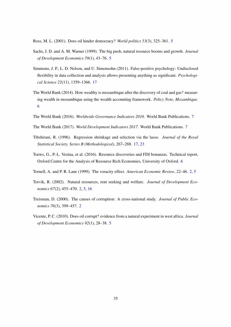
Ross, M. L. (2001). Does oil hinder democracy? World politics 53(3), 325–361. 5

Sachs, J. D. and A. M. Warner (1999). The big push, natural resource booms and growth. Journal

of Development Economics 59(1), 43–76. 5

Simmons, J. P., L. D. Nelson, and U. Simonsohn (2011). False-positive psychology: Undisclosed

flexibility in data collection and analysis allows presenting anything as significant. Psychologi-

cal Science 22(11), 1359–1366. 17

The World Bank (2014). How wealthy is mozambique after the discovery of coal and gas? measur-

ing wealth in mozambique using the wealth accounting framework. Policy Note, Mozambique.

6

The World Bank (2016). Worldwide Governance Indicators 2016. World Bank Publications. 7

The World Bank (2017). World Development Indicators 2017. World Bank Publications. 7

Tibshirani, R. (1996). Regression shrinkage and selection via the lasso. Journal of the Royal

Statistical Society. Series B (Methodological), 267–288. 17, 23

Toews, G., P.-L. Vezina, et al. (2016). Resource discoveries and FDI bonanzas. Technical report,

Oxford Centre for the Analysis of Resource Rich Economies, University of Oxford. 6

Tornell, A. and P. R. Lane (1999). The voracity effect. American Economic Review, 22–46. 2, 5

Torvik, R. (2002). Natural resources, rent seeking and welfare. Journal of Development Eco-

nomics 67(2), 455–470. 2, 5, 16

Treisman, D. (2000). The causes of corruption: A cross-national study. Journal of Public Eco-

nomics 76(3), 399–457. 2

Vicente, P. C. (2010). Does oil corrupt? evidence from a natural experiment in west africa. Journal

of Development Economics 92(1), 28–38. 5

35

Figure 1: Timeline

Note. The timeline presents the activities of the project from the implementation of the baseline survey in August 2016 to thecompletion of all SCAs in December 2017. The lower part of the figure presents the detailed timeline of the endline activities.

36

Figure 2: Information Leaflet

Note. The information leaflet was designed by the research team in collaboration with a large number of governmentaland non-governmental organizations.

37

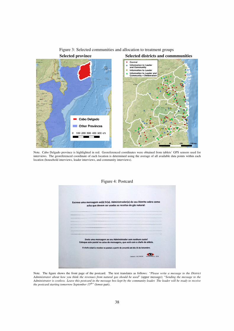
Figure 3: Selected communities and allocation to treatment groupsSelected province Selected districts and commmunities

Note. Cabo Delgado province is highlighted in red. Georeferenced coordinates were obtained from tablets’ GPS sensors used forinterviews. The georeferenced coordinate of each location is determined using the average of all available data points within eachlocation (household interviews, leader interviews, and community interviews).

Figure 4: Postcard

Note. The figure shows the front page of the postcard. The text translates as follows: “Please write a message to the DistrictAdministrator about how you think the revenues from natural gas should be used” (upper message); “Sending the message to theAdministrator is costless. Leave this postcard in the message box kept by the community leader. The leader will be ready to receivethe postcard starting tomorrow September 15th” (lower part).

38

Figure 5: Raven’s test distributions

Note. The left panel shows a comparison in the distribution of Raven’s test scores among community members and the average Raven’sTest Score among the individuals selected for the taskforce activity. The right panel shows the distributions of the difference betweenthe leader’s taskforce and the community average in the control group and the two treatment groups.

Figure 6: Aggregation: results

-.4

-.2

0

.2

.4

.6

T1 T2

Leader's knowledge Leader's perceived benefitsElite capture Rent-seeking among leadersViolence

Community-level outcomes

-.4

-.2

0

.2

.4

.6

T1 T2

Citizen's knowledge Citizen's perceived benefitsRent-seeking among citizens Citizen's mobilizationTrust and accountability Self-reported violence

Citizen-level outcomes

Note. Estimates based on OLS regressions (see equation 1). Confidence intervals are built using statistical significance at the 10% level,and standard errors clustered at the community level when employing citizen-level outcomes. The specifications include communityand household-level controls (for citizen-level outcomes) or community-level controls (for community-level outcomes). The full listof controls is presented in Section 7. Outcomes are grouped in indices that are built using the Kling et al. (2007) procedure. Outcomesare first normalized in standardized units to study mean effect sizes of the indices relative to the standard deviation of the control groupand then averaged within each category.

39

Tabl

e1:

Lea

ders

’kno

wle

dge

and

perc

eptio

nsab

outt

hena

tura

lgas

disc

over

yD

ep.V

ar.:

Awar

enes

sK

now

ledg

eSa

lienc

ePe

rcei

ved

bene

fitto

...co

mm

unity

hous

ehol

dSa

mpl

e:A

llA

llA

llA

llA

llA

llR

espo

nden

tsaw

are

ofth

edi

scov

ery

(1)

(2)

(3)

(4)

(5)

(6)

(7)

(8)

(T1)

Info

rmat

ion

toL

eade

r0.

043*

*0.

043*

*0.

034*

0.03

8**

0.03

50.

045

0.01

60.

014

(0.0

20)

(0.0

19)

(0.0

18)

(0.0

18)

(0.0

86)

(0.0

87)

(0.0

65)

(0.0

79)

[0.1

1-0.

18]

[0.1

0-0.

16]

[0.1

7-0.

31]

[0.1

1-0.

18]

[0.9

5-0.

99]

[0.9

1-0.

99]

[0.9

5-0.

99]

[0.9

5-0.

99]

(T2)

Info

rmat

ion

toL

eade

rand

Citi

zens

0.04

9***

0.05

2***

0.05

4***

0.05

6***

0.33

4***

0.34

0***

-0.0

08-0

.042

(0.0

18)

(0.0

18)

(0.0

17)

(0.0

16)

(0.0

78)

(0.0

79)

(0.0

59)

(0.0

72)

[0.0

3-0.

05]

[0.0

2-0.

03]

[0.0

1-0.

01]

[0.0

1-0.

01]

[0.0

0-0.

00]

[0.0

0-0.

00]

[0.8

9-0.

99]

[0.7

2-0.

97]

Obs

erva

tions

206

203

206

203

206

203

204

204

R2

0.10

90.

146

0.20

00.

273

0.33

90.

333

0.15

40.

125

Mea

n(c

ontr

olgr

oup)

0.96

40.

964

0.62

70.

627

0.29

10.

291

0.86

80.

830

T1

=T

2(p

-val

ue)

0.73

80.

648

0.24

50.

255

0.00

00.

000

0.67

10.

430

T1

=T

2(a

dj.p

-val

ue,r

ow-l

evel

)0.

780

0.78

00.

503

0.50

30.

001

0.00

10.

780

0.66

0T

1=

T2

(adj

.p-v

alue

,tab

le-l

evel

)0.

989

0.98

60.

754

0.75

80.

003

0.00

50.

988

0.91

0L

agge

dde

pend

entv

aria

ble

No

Yes

No

Yes

No

Yes

No

No

Not

e.E

stim

ates

base

don

OL

Sre

gres

sion

s(s

eeeq

uatio

ns1

and

2).

***

p<0.

01,*

*p<

0.05

,*p<

0.1.

Stan

dard

erro

rsar

ere

port

edin

pare

nthe

sis.

P-va

lues

adju

sted

for

mul

tiple

hypo

thes

iste

stin

gar

epr

esen

ted

inbr

acke

ts(s

eeSe

ctio

n7

ford

etai

ls).

The

first

p-va

lue

corr

espo

nds

tojo

intly

test

ing

coef

ficie

nts

grou

ped

byro

ws

(row

-lev

el),

the

seco

ndp-

valu

eco

rres

pond

sto

join

tlyte

stin

gth

atT

1,T

2an

dT

1-T

2ar

edi

ffer

entf

rom

zero

(tab

le-l

evel

).C

olum

ns(1

),(3

),(5

)and

(7)–

(8)p

rese

ntes

timat

esus

ing

equa

tion

(1).

Col

umns

(2),

(4),

(6)p

rese

ntes

timat

esus

ing

equa

tion

(2),

incl

udin

gth

ela

gged

valu

eof

the

depe

nden

tvar

iabl

e.D

epen

ding

onth

eco

lum

n,th

ede

pend

entv

aria

bles

are

defin

edby

the

follo

win

g:(1

)–(2

)Aw

aren

ess:

indi

cato

rvar

iabl

eeq

ualt

o1

ifth

ere

spon

dent

repo

rts

havi

nghe

ard

abou

tthe

natu

ralg

asdi

scov

ery;

(3)–

(4)K

now

ledg

e:in

dex

built

aver

agin

g15

indi

cato

rvar

iabl

esre

late

dto

know

ledg

eab

outt

helo

catio

nof

the

disc

over

y,w

heth

erex

plor

atio

nha

sst

arte

d,w

heth

erth

ego

vern

men

tis

rece

ivin

gre

venu

es,w

hen

extr

actio

nis

expe

cted

tost

art,

and

whi

chfir

ms

are

invo

lved

;(5)

–(6)

Salie

nce:

indi

cato

rvar

iabl

eeq

ualt

o1

whe

ther

the

resp

onde

ntus

eth

ew

ord

“gas

”w

hen

aske

dab

outt

heth

ree

maj

orev

ents

inth

edi

stri

ctin

the

last

5ye

ars;

(7)P

erce

ived

bene

fitto

com

mun

ity:

indi

cato

rvar

iabl

eeq

ualt

o1

ifth

ere

spon

dent

agre

esor

fully

agre

esth

atth

eco

mm

unity

will

bene

fitfr

omna

tura

lga

s;(8

)Per

ceiv

edbe

nefit

toho

useh

old:

indi

cato

rvar

iabl

eeq

ualt

o1

ifth

ere

spon

dent

agre

esor

fully

agre

esth

athi

sho

useh

old

will

bene

fitfr

omna

tura

lgas

.In

colu

mns

(7)a

nd(8

),th

esa

mpl

eis

rest

rict

edto

resp

onde

nts

awar

eof

the

natu

ralg

asdi

scov

ery.

All

spec

ifica

tions

incl

ude

com

mun

ityan

dle

ader

-lev

elco

ntro

ls.T

hefu

lllis

tofc

ontr

ols

ispr

esen

ted

inSe

ctio

n7.

40

Tabl

e2:

Citi

zens

’kno

wle

dge,

and

perc

eptio

nsab

outt

hena

tura

lgas

disc

over

yD

ep.V

ar.:

Awar

enes

sK

now

ledg

eSa

lienc

ePe

rcei

ved

bene

fitto

...co

mm

unity

hous

ehol

dSa

mpl

e:A

llA

llA

llA

llA

llA

llR

espo

nden

tsaw

are

ofth

edi

scov

ery

(1)

(2)

(3)

(4)

(5)

(6)

(7)

(8)

(T1)

Info

rmat

ion

toL

eade

r-0

.004

-0.0

03-0

.002

-0.0

010.

053*

0.06

6**

-0.0

090.

015

(0.0

32)

(0.0

33)

(0.0

20)

(0.0

20)

(0.0

29)

(0.0

32)

(0.0

31)

(0.0

31)

[0.9

9-0.

99]

[1.0

0-1.

00]

[1.0

0-1.

00]

[1.0

0-1.

00]

[0.2

5-0.

27]

[0.1

8-0.

25]

[0.9

9-0.

99]

[0.9

7-0.

97]

(T2)

Info

rmat

ion

toL

eade

rand

Citi

zens

0.25

4***

0.25

1***

0.17

3***

0.16

9***

0.23

3***

0.23

8***

0.04

4*0.

071*

**(0

.023

)(0

.023

)(0

.016

)(0

.015

)(0

.027

)(0

.029

)(0

.023

)(0

.026

)[0

.00-

0.00

][0

.00-

0.00

][0

.00-

0.00

][0

.00-

0.00

][0

.00-

0.00

][0

.00-

0.00

][0

.06-

0.27

][0

.02-

0.07

]

Obs

erva

tions

2072

1886

2072

1886

2077

1890

1592

1573

R2

0.25

10.

272

0.36

80.

396

0.15

70.

154

0.13

50.

114

Mea

n(c

ontr

olgr

oup)

0.68

10.

671

0.45

70.

449

0.18

90.

182

0.77

90.

692

T1

=T

2(p

-val

ue)

0.00

00.

000

0.00

00.

000

0.00

00.

000

0.04

60.

050

T1

=T

2(a

dj.p

-val

ue,r

ow-l

evel

)0.

001

0.00

10.

001

0.00

10.

001

0.00

10.

088

0.08

8T

1=

T2

(adj

.p-v

alue

,tab

le-l

evel

)0.

001

0.00

10.

001

0.00

10.

001

0.00

10.

264

0.26

7L

agge

dde

pend

entv

aria

ble

No

Yes

No

Yes

No

Yes

No

No

Not

e.E

stim

ates

base

don

OL

Sre

gres

sion

s(s

eeeq

uatio

ns1

and

2).*

**p<

0.01

,**

p<0.

05,*

p<0.

1.St

anda

rder

rors

are

repo

rted

inpa

rent

hesi

san

dcl

uste

red

atth

eco

mm

unity

leve

l.P-

valu

esad

just

edfo

rmul

tiple

hypo

thes

iste

stin

gar

epr

esen

ted

inbr

acke

ts(s

eeSe

ctio

n7

ford

etai

ls).

The

first

p-va

lue

corr

espo

nds

tojo

intly

test

ing

coef

ficie

nts

grou

ped

byro

ws

(row

-lev

el),

the

seco

ndp-

valu

eco

rres

pond

sto

join

tlyte

stin

gth

atT

1,T

2an

dT

1-T

2ar

edi

ffer

entf

rom

zero

(tab

le-l

evel

).C

olum

ns(1

),(3

),(5

)and

(7)–

(8)p

rese

ntes

timat

esus

ing

equa

tion

(1).

Col

umns

(2),

(4),

(6)p

rese

ntes

timat

esus

ing

equa

tion

(2),

incl

udin

gth

ela

gged

valu

eof

the

depe

nden

tvar

iabl

e.D

epen

ding

onth

eco

lum

n,th

ede

pend

entv

aria

bles

are

defin

edby

the

follo

win

g:(1

)–(2

)Aw

aren

ess:

indi

cato

rvar

iabl

eeq

ualt

o1

ifth

ere

spon

dent

repo

rts

havi

nghe

ard

abou

tthe

natu

ralg

asdi

scov

ery;

(3)–

(4)

Kno

wle

dge:

inde

xbu

iltav

erag

ing

15in

dica

tor

vari

able

sre

late

dto

know

ledg

eab

outt

helo

catio

nof

the

disc

over

y,w

heth

erex

plor

atio

nha

sst

arte

d,w

heth

erth

ego

vern

men

tis

rece

ivin

gre

venu

es,w

hen

extr

actio

nis

expe

cted

tost

art,

and

whi

chfir

ms

are

invo

lved

;(5)

–(6)

Salie

nce:

indi

cato

rva

riab

leeq

ualt

o1

whe

ther

the

resp

onde

ntus

eth

ew

ord

“gas

”w

hen

aske

dab

outt

heth

ree

maj

orev

ents

inth

edi

stri

ctin

the

last

5ye

ars;

(7)

Perc

eive

dbe

nefit

toco

mm

unity

:in

dica

tor

vari

able

equa

lto

1if

the

resp

onde

ntag

rees

orfu

llyag

rees

that

the

com

mun

ityw

illbe

nefit

from

natu

ralg

as;(

8)Pe

rcei

ved

bene

fitto

hous

ehol

d:in

dica

tor

vari

able

equa

lto

1if

the

resp

onde

ntag

rees

orfu

llyag

rees

that

his/

her

hous

ehol

dw

illbe

nefit

from

natu

ralg

as.

Inco

lum

ns(7

)and

(8),

the

sam

ple

isre

stri

cted

tore

spon

dent

saw

are

ofth

ena

tura

lgas

disc

over

y.A

llsp

ecifi

catio

nsin

clud

eco

mm

unity

and

hous

ehol

d-le

velc

ontr

ols.

The

full

listo

fcon

trol

sis

pres

ente

din

Sect

ion

7.

41

Tabl

e3:

Elit

eca

ptur

eD

ep.V

ar.

Att

itude

stow

ards

Zin

cro

oftil

esFu

ndsf

orm

eetin

gsTa

skfo

rce

activ

ityTr

ustg

ame

corr

uptio

nE

lite

deci

ded

Priv

ate

usag

eA

ppro

pria

ted

fund

sSh

are

ap-

prop

riat

edAv

gR

aven

’ssc

ores

Mid

perf

orm

ers

sele

cted

Men

sele

cted

Lea

der

kept

(1)

(2)

(3)

(4)

(5)

(6)

(7)

(8)

(9)

(10)

(T1)

Info

rmat

ion

toL

eade

r0.

099*

*0.

099*

*-0

.067

-0.1

010.

271*

**0.

144*

**0.

281

0.19

3**

0.07

3*0.

032

(0.0

40)

(0.0

40)

(0.0

79)

(0.0

75)

(0.0

95)

(0.0

53)

(0.3

14)

(0.0

97)

(0.0

41)

(0.0

38)

[0.0

9-0.

23]

[0.0

9-0.

23]

[0.7

1-0.

99]

[0.5

1-0.

89]

[0.0

4-0.

10]

[0.0

6-0.

15]

[0.7

1-0.

99]

[0.2

5-0.

54]

[0.3

0-0.

67]

[0.7

1-0.

99]

(T2)

Info

rmat

ion

toL

eade

rand

Citi

zens

0.06

5*0.

069*

-0.1

87**

*-0

.084

0.12

00.

005

0.20

40.

122

-0.0

040.

026

(0.0

36)

(0.0

37)

(0.0

71)

(0.0

68)

(0.0

86)

(0.0

48)

(0.2

83)

(0.0

87)

(0.0

37)

(0.0

34)

[0.4

1-0.

67]

[0.3

6-0.

61]

[0.0

7-0.

17]

[0.6

7-0.

92]

[0.6

7-0.

88]

[0.9

9-1.

00]

[0.8

9-0.

99]

[0.6

7-0.

88]

[0.9

9-1.

00]

[0.8

9-0.

99]

Obs

erva

tions

206

203

206

206

205

205

206

206

206

206

R2

0.17

10.

171

0.29

50.

209

0.16

90.

235

0.16

90.

145

0.24

30.

119

Mea

n(c

ontr

olgr

oup)

0.07

30.

073

0.85

50.

255

0.47

30.

227

3.51

60.

491

0.78

20.

605

T1

=T

2(p

-val

ue)

0.34

30.

413

0.09

50.

806

0.07

90.

004

0.78

40.

422

0.03

80.

861

T1

=T

2(a

dj.p

-val

ue,r

ow-l

evel

)0.

870

0.91

70.

406

0.98

50.

392

0.03

80.

985

0.91

70.

220

0.98

5T

1=

T2

(adj

.p-v

alue

,tab

le-l

evel

)0.

984

0.99

20.

720

0.99

90.

674

0.09

70.

999

0.99

20.

472

0.99

9L

agge

dde

pend

entv

aria

ble

No

Yes

No

No

No

No

No

No

No

No

Not

e.E

stim

ates

base

don

OL

Sre

gres

sion

s(s

eeeq

uatio

ns1

and

2).*

**p<

0.01

,**

p<0.

05,*

p<0.

1.St

anda

rder

rors

are

repo

rted

inpa

rent

hesi

s.P-

valu

esad

just

edfo

rmul

tiple

hypo

thes

iste

stin

gar

epr

esen

ted

inbr

acke

ts(s

eeSe

ctio

n7

ford

etai

ls).

The

first

p-va

lue

corr

espo

nds

tojo

intly

test

ing

coef

ficie

nts

grou

ped

byro

ws

(row

-lev

el),

the

seco

ndp-

valu

eco

rres

pond

sto

join

tlyte

stin

gth

atT

1,T

2an

dT

1-T

2ar

edi

ffer

entf

rom

zero

(tab

le-l

evel

).C

olum

ns(1

),(3

)–(1

0)pr

esen

test

imat

esus

ing

equa

tion

(1).

Col

umn

(2)p

rese

nts

estim

ates

usin

geq

uatio

n(2

),in

clud

ing

the

lagg

edva

lue

ofth

ede

pend

entv

aria

ble.

Dep

endi

ngon

the

colu

mn,

the

depe

nden

tvar

iabl

esar

ede

fined

byth

efo

llow

ing:

(1)–

(2)A

ttitu

des

tow

ards

corr

uptio

n:av

erag

ebe

twee

nan

indi

cato

rvar

iabl

eeq

ualt

o1

ifth

ele

ader

agre

esw

ithth

est

atem

ent“

the

best

way

toov

erco

me

prob

lem

sis

topa

ybr

ibes

”an

dan

indi

cato

rvar

iabl

eeq

ualt

o1

ifth

ele

ader

wou

ldde

man

da

job

forh

im/h

erse

lfw

hen

aske

d“I

mag

ine

that

you

had

the

oppo

rtun

ityto

have

am

eetin

gw

ithth

eG

over

noro

fCab

oD

elga

doan

dth

atyo

uco

uld

mak

ea

requ

est.

Plea

sete

llm

ew

haty

ouw

ould

requ

est.”

ForZ

inc

roof

tiles

[see

5.2.

1],(

3)E

lite

deci

ded:

dum

my

that

take

sva

lue

1if

the

elite

deci

ded

the

use

ofth

ezi

ncsh

eets

,and

0if

the

deci

sion

was

mad

eby

the

com

mun

ity(s

elf-

repo

rted

byth

ele

ader

);(4

)Priv

ate

usag

e:ob

serv

edus

eof

zinc

s,ta

kes

valu

e1

ifus

edfo

rind

ivid

ualp

urpo

ses,

0if

used

fort

heco

mm

unity

orno

tuse

dye

t.Fo

rFun

dsfo

rMee

tings

[see

5.2.

2],(

5)A

ppro

pria

ted

fund

s:in

dica

tor

for

whe

ther

the

lead

erus

edle

ssth

an350

Met

icai

sou

tof

400

for

mee

ting;

(6)

Shar

eap

prop

riat

ed:

shar

edi

ffer

ence

betw

een

avai

labl

efu

nds

and

expe

nses

duri

ngth

em

eetin

g.Fo

rth

eTa

skfo

rce

activ

ity[s

ee5.

2.3]

,(7)

Ave

rage

scor

eon

Rav

en’s

test

ofin

divi

dual

sch

osen

byle

ader

;(8)

Mid

perf

orm

ers

sele

cted

:in

dica

tor

vari

able

for

2nd-4

thqu

intil

ein

the

sam

ple

dist

ribu

tion

ofdi

ffer

ence

betw

een

aver

age

test

scor

eof

indi

vidu

als

chos

enby

lead

eran

dav

erag

ete

stsc

ore

ofre

pres

enta

tive

indi

vidu

als

sele

cted

for

the

surv

eyat

the

leve

lof

the

com

mun

ity;

(9)

Men

sele

cted

:pe

rcen

tage

ofw

omen

chos

enby

lead

erfo

rthe

Rav

en’s

test

.For

the

Trus

tGam

e[s

ee5.

3.1]

,(10

)Lea

derk

ept:

amou

ntle

ader

kept

inTr

ustg

ame

(res

cale

dbe

twee

n0

and

1).A

llsp

ecifi

catio

nsin

clud

eco

mm

unity

and

lead

er-l

evel

cont

rols

.The

full

listo

fcon

trol

sis

pres

ente

din

Sect

ion

7.

42

Tabl

e4:

Ren

t-se

ekin

gR

ent-

seek

ing

amon

glo

call

eade

rsR

ent-

seek

ing

amon

gci

tizen

s

Dep

.Var

.In

tera

ctio

nw

ithA

uctio

nR

ent-

seek

ing

Inte

ract

ion

with

...A

uctio

nR

ent-

seek

ing

gam

eot

her

polit

ical

Bid

for

Deg

ree

ofch

iefs

othe

rpo

litic

alSh

are

bid

Any

gift

Gift

ssen

tle

ader

sm

eetin

gR

Sle

ader

sto

mee

ting

sent

(1)

(2)

(3)

(4)

(5)

(6)

(7)

(8)

(9)

(10)

(11)

(T1)

Info

rmat

ion

toL

eade

r0.

161*

**0.

162*

**0.

058

0.04

40.

100*

**0.

092*

**-0

.007

0.00

10.

025*

*0.

059*

*0.

040*

(0.0

53)

(0.0

53)

(0.1

20)

(0.0

52)

(0.0

34)

(0.0

35)

(0.0

38)

(0.0

34)

(0.0

12)

(0.0

26)

(0.0

23)

[0.0

1-0.

03]

[0.0

1-0.

03]

[0.6

2-0.

93]

[0.6

2-0.

88]

[0.0

3-0.

06]

[0.0

6-0.

13]

[0.9

3-0.

99]

[0.9

7-0.

99]

[0.1

4-0.

36]

[0.1

0-0.

27]

[0.2

0-0.

56]

(T2)

Info

rmat

ion

toL

eade

rand

Citi

zens

0.11

6**

0.11

4**

0.06

70.

002

0.02

70.

022

0.01

00.

009

0.00

50.

043*

0.03

1(0

.048

)(0

.048

)(0

.108

)(0

.047

)(0

.028

)(0

.029

)(0

.032

)(0

.030

)(0

.010

)(0

.025

)(0

.021

)[0

.06-

0.12

][0

.06-

0.12

][0

.75-

0.89

][0

.97-

1.00

][0

.76-

0.94

][0

.85-

0.97

][0

.90-

0.99

][0

.90-

0.99

][0

.90-

0.99

][0

.37-

0.55

][0

.52-

0.71

]

Obs

erva

tions

206

203

206

204

2077

1890

2077

1890

2077

2027

2027

R2

0.18

80.

212

0.19

80.

131

0.10

10.

101

0.11

80.

133

0.02

10.

026

0.07

8M

ean

(con

trol

grou

p)0.

818

0.81

84.

217

0.24

30.

531

0.53

10.

474

0.45

10.

499

0.88

00.

408

T1

=T

2(p

-val

ue)

0.35

10.

311

0.93

90.

372

0.01

10.

022

0.60

80.

789

0.02

50.

361

0.61

5T

1=

T2

(adj

.p-v

alue

,row

-lev

el)

0.68

10.

642

0.93

10.

681

0.06

10.

106

0.86

30.

863

0.10

60.

743

0.86

3T

1=

T2

(adj

.p-v

alue

,tab

le-l

evel

)0.

871

0.83

90.

997

0.87

10.

153

0.26

80.

986

0.98

60.

275

0.94

80.

986

Lag

ged

Dep

ende

ntV

aria

ble

No

Yes

No

No

No

Yes

No

Yes

No

No

No

Not

e.E

stim

ates

base

don

OL

Sre

gres

sion

s.**

*p<

0.01

,**

p<0.

05,*

p<0.

1.St

anda

rder

rors

are

repo

rted

inpa

rent

hesi

s.P-

valu

esad

just

edfo

rm

ultip

lehy

poth

esis

test

ing

are

pres

ente

din

brac

kets

(see

Sect

ion

7fo

rde

tails

).T

hefir

stp-

valu

eco

rres

pond

sto

join

tlyte

stin

gco

effic

ient

sgr

oupe

dby

row

s(r

ow-l

evel

),th

ese

cond

p-va

lue

corr

espo

nds

tojo

intly

test

ing

that

T1,

T2

and

T1-

T2

are

diff

eren

tfro

mze

ro(t

able

-lev

el).

Test

ing

ispe

rfor

med

sepa

rate

lyfo

rcol

umns

(1)–

(4)a

ndco

lum

ns(5

)–(1

1).C

olum

ns(1

)–(9

)pre

sent

estim

ates

usin

geq

uatio

n(1

).C

olum

ns(1

)–(3

)ref

erto

outc

omes

rela

ted

tore

nt-s

eeki

ngam

ong

loca

llea

ders

,whi

leco

lum

ns(4

)–(9

)re

fer

tore

nt-s

eeki

ngam

ong

citiz

ens.

For

loca

llea

ders

,dep

endi

ngon

the

colu

mn,

the

depe

nden

tvar

iabl

esar

ede

fined

byth

efo

llow

ing:

(1)–

(2)

Inte

ract

ion

with

othe

rpo

litic

alle

ader

s:in

dica

tor

vari

able

equa

lto

1if

the

lead

erre

port

edha

ving

talk

edor

calle

dan

othe

rpo

litic

alle

ader

inth

e6

mon

ths

prev

ious

toth

ein

terv

iew

;fo

rth

eA

uctio

nac

tivity

[see

5.2.

4],(

3)B

idfo

rm

eetin

g:lo

gam

ount

bid

for

the

mee

ting

with

adm

inis

trat

or.

For

the

Ren

t-se

ekin

gga

me

[see

5.3.

2],(

4)D

egre

eof

rent

-see

king

:si

zeof

gift

chos

enby

lead

erin

rent

-see

king

gam

e,w

hich

coul

dra

nge

from

0(l

owes

tren

t-se

ekin

g)to

1(f

ullr

ent-

seek

ing)

.Fo

rC

itize

ns,d

epen

ding

onth

eco

lum

n,th

ede

pend

entv

aria

bles

are

defin

edby

the

follo

win

g:(5

)–(6

)In

tera

ctio

nw

ithch

iefs

:in

dica

tor

vari

able

equa

lto

1if

the

pers

onre

port

edha

ving

talk

edor

havi

ngca

lled

the

loca

llea

ders

inth

e6

mon

ths

prev

ious

toth

ein

terv

iew

;(7)

–(8)

Inte

ract

ion

with

othe

rpo

litic

alle

ader

s:in

dica

tor

vari

able

equa

lto

1if

the

pers

onre

port

edha

ving

talk

edor

havi

ngca

lled

toan

othe

rpo

litic

alle

ader

inth

e6

mon

ths

prev

ious

toth

ein

terv

iew

.Fo

rth

eM

eetin

g−

Trai

ning

Auc

tion

activ

ity[s

ee5.

2.4]

,(9)

Shar

ebi

dto

mee

ting:

shar

eof

tota

lbid

sal

loca

ted

tom

eetin

gth

ead

min

istr

ator

.For

the

Ren

t-se

ekin

gG

ame

[see

5.3.

2],(

10)A

nygi

ftse

nt:i

ndic

ator

vari

able

forw

heth

erth

epa

rtic

ipan

tsen

tany

toke

nsas

gift

tole

ader

,(11

)Gif

tsse

nt:n

umbe

rofg

iftt

oken

s(r

esca

led

betw

een

0an

d1)

sent

tole

ader

.Spe

cific

atio

nsin

colu

mns

(1)–

(3)i

nclu

deco

mm

unity

and

lead

er-l

evel

cont

rols

.Spe

cific

atio

nsin

colu

mns

(4)–

(9)i

nclu

deco

mm

unity

and

hous

ehol

d-le

velc

ontr

ols.

The

full

listo

fcon

trol

sis

pres

ente

din

Sect

ion

7.L

agge

dD

epen

dent

vari

able

isno

tinc

lude

d.

43

Tabl

e5:

Citi

zens

’mob

iliza

tion

Dep

.Var

.C

omm

unity

mee

tings

Mat

chin

ggr

ants

Com

mun

itym

eetin

gs(M

G)

Publ

icgo

odsg

ame

Att

enda

nce

Awar

enes

sC

ontr

ibut

edA

mou

ntA

tten

danc

eVo

ting

Con

trib

utio

n(s

elf-

repo

rted

)co

ntri

bute

d(1

)(2

)(3

)(4

)(5

)(6

)(7

)(8

)

(T1)

Info

rmat

ion

toL

eade

r0.

008

0.00

40.

024

0.05

80.

152

0.01

7-0

.030

-0.0

03(0

.021

)(0

.022

)(0

.036

)(0

.048

)(0

.191

)(0

.011

)(0

.033

)(0

.020

)[0

.94-

1.00

][0

.98-

1.00

][0

.91-

0.99

][0

.72-

0.93

][0

.91-

0.98

][0

.59-

0.80

][0

.87-

0.97

][0

.98-

1.00

]

(T2)

Info

rmat

ion

toL

eade

rand

Citi

zens

0.03

8**

0.03

9**

0.10

8***

0.15

2***

0.47

8***

0.00

50.

015

0.00

1(0

.015

)(0

.016

)(0

.029

)(0

.046

)(0

.180

)(0

.010

)(0

.030

)(0

.020

)[0

.08-

0.23

][0

.08-

0.24

][0

.01-

0.02

][0

.01-

0.04

][0

.06-

0.17

][0

.95-

1.00

][0

.95-

1.00

][0

.96-

1.00

]

Obs

erva

tions

2019

1803

2072

1510

1510

184

196

2027

R2

0.07

00.

086

0.10

00.

075

0.06

50.

266

0.09

30.

057

Mea

n(c

ontr

olgr

oup)

0.89

90.

892

0.70

40.

223

0.89

20.

025

0.01

90.

448

T1

=T

2(p

-val

ue)

0.10

10.

076

0.00

40.

032

0.07

00.

237

0.12

30.

770

T1

=T

2(a

dj.p

-val

ue,r

ow-l

evel

)0.

397

0.36

60.

050

0.20

60.

366

0.50

70.

397

0.76

5T

1=

T2

(adj

.p-v

alue

,tab

le-l

evel

)0.

734

0.64

00.

095

0.39

90.

628

0.93

40.

783

0.99

5L

agge

dD

epen

dent

Var

iabl

eN

oY

esN

oN

oN

oN

oN

oN

o

Not

e.E

stim

ates

base

don

OL

Sre

gres

sion

s.**

*p<

0.01

,**

p<0.

05,*

p<0.

1.St

anda

rder

rors

are

repo

rted

inpa

rent

hesi

san

dcl

uste

red

atth

eco

mm

unity

leve

l,ex

cept

inco

lum

ns(6

)an

d(7

).P-

valu

esad

just

edfo

rm

ultip

lehy

poth

esis

test

ing

are

pres

ente

din

brac

kets

(see

Sect

ion

7fo

rde

tails

).T

hefir

stp-

valu

eco

rres

pond

sto

join

tlyte

stin

gco

effic

ient

sgr

oupe

dby

row

s(r

ow-l

evel

),th

ese

cond

p-va

lue

corr

espo

nds

tojo

intly

test

ing

that

T1,

T2

and

T1-

T2

are

diff

eren

tfro

mze

ro(t

able

-lev

el).

Col

umns

(1),

(3)–

(8)

pres

ente

stim

ates

usin

geq

uatio

n(1

).C

olum

n(2

)pr

esen

tses

timat

esus

ing

equa

tion

(2),

incl

udin

gth

ela

gged

valu

eof

the

depe

nden

tvar

iabl

e.D

epen

ding

onth

eco

lum

n,th

ede

pend

entv

aria

bles

are

defin

edby

the

follo

win

g:(1

)–(2

)Com

mun

itym

eetin

gsat

tend

ance

(sel

f-re

port

ed):

indi

cato

rva

riab

leeq

ualt

o1

ifth

eci

tizen

atte

nded

atle

asto

neco

mm

unity

mee

ting

inth

ela

st12

mon

ths.

For

mat

chin

ggr

ants

activ

ity[s

ee5.

2.5]

:(3

)A

war

enes

s:in

dica

tor

vari

able

equa

lto

1if

the

citiz

enhe

ard

abou

tthe

activ

ity;(

4)C

ontr

ibut

ed:

indi

cato

rva

riab

leeq

ualt

o1

ifth

eci

tizen

repo

rted

cont

ribu

ting

apo

sitiv

eam

ount

;(5)

Am

ount

cont

ribu

ted:

log

ofse

lf-r

epor

ted

cont

ribu

tion

inm

atch

ing

activ

ity;(

6)A

ttend

ance

:(ob

serv

ed)s

hare

ofad

ults

inth

eco

mm

unity

who

atte

nded

the

com

mun

itym

eetin

gw

here

the

part

icip

atio

nin

the

mat

chin

ggr

ants

(MG

)act

ivity

was

disc

usse

d;(7

)Vot

ing:

indi

cato

rvar

iabl

eeq

ualt

o1

ifth

ede

cisi

onin

the

com

mun

itym

eetin

gw

asde

term

ined

byvo

ting

(obs

erve

d).

For

publ

icgo

ods

gam

e[s

ee5.

3.3]

:(8

)C

ontr

ibut

ion:

cont

ribu

tion

(res

cale

dbe

twee

n0

and

1)in

publ

icgo

ods

gam

e.Sp

ecifi

catio

nsin

colu

mns

(1)–

(5)

and

(8)

incl

ude

com

mun

ityan

dho

useh

old-

leve

lcon

trol

s.Sp

ecifi

catio

nsin

colu

mns

(6)

and

(7)

incl

ude

com

mun

ityan

dle

ader

-lev

elco

ntro

ls.

The

full

listo

fco

ntro

lsis

pres

ente

din

Sect

ion

7.

44

Tabl

e6:

Trus

tand

dem

and

forp

oliti

cala

ccou

ntab

ility

Dep

.Var

.Tr

ust(

self-

repo

rted

)Su

rvey

-bas

edac

coun

tabi

lity

Trus

tgam

ePo

stca

rdAv

erag

etr

ust

On

lead

ers

Voic

eou

tsid

ePo

litic

alA

mou

ntD

esir

eto

sent

pers

onal

lykn

own

the

com

mun

ityac

coun

tabi

lity

sent

puni

sh(1

)(2

)(3

)(4

)(5

)(6

)(7

)(8

)(9

)(1

0)

(T1)

Info

rmat

ion

toL

eade

r-0

.052

*-0

.054

*-0

.033

-0.0

33-0

.007

0.02

5-0

.136

**0.

029

0.02

50.

034

(0.0

27)

(0.0

28)

(0.0

21)

(0.0

23)

(0.0

48)

(0.0

53)

(0.0

66)

(0.0

18)

(0.0

37)

(0.0

32)

[0.3

5-0.

57]

[0.3

5-0.

57]

[0.5

2-0.

80]

[0.5

2-0.

85]

[0.8

8-1.

00]

[0.8

0-0.

99]

[0.3

0-0.

49]

[0.5

2-0.

81]

[0.8

0-0.

98]

[0.6

9-0.

96]

(T2)

Info

rmat

ion

toL

eade

rand

Citi

zens

0.02

20.

025

0.05

1***

0.05

0***

0.08

7**

0.12

3***

0.02

20.

014

0.01

70.

030

(0.0

23)

(0.0

23)

(0.0

15)

(0.0

17)

(0.0

39)

(0.0

44)

(0.0

59)

(0.0

18)

(0.0

32)

(0.0

21)

[0.8

3-0.

98]

[0.7

8-0.

96]

[0.0

1-0.

03]

[0.0

3-0.

09]

[0.1

6-0.

39]

[0.0

4-0.

15]

[0.8

6-1.

00]

[0.8

4-0.

98]

[0.8

6-0.

99]

[0.5

9-0.

85]

Obs

erva

tions

2035

1754

1958

1614

1983

1718

1997

2027

2007

1891

R2

0.08

80.

124

0.13

20.

153

0.06

00.

068

0.08

00.

114

0.03

70.

087

Mea

n(c

ontr

olgr

oup)

2.21

82.

214

2.85

12.

848

2.49

42.

463

3.83

40.

405

0.39

80.

881

T1

=T

2(p

-val

ue)

0.00

30.

002

0.00

00.

000

0.02

20.

035

0.00

90.

378

0.80

50.

864

T1

=T

2(a

dj.p

-val

ue,r

ow-l

evel

)0.

040

0.02

50.

001

0.00

20.

140

0.18

30.

083

0.78

50.

963

0.96

3T

1=

T2

(adj

.p-v

alue

,tab

le-l

evel

)0.

090

0.05

50.

001

0.00

70.

365

0.47

20.

193

0.97

60.

995

0.99

5L

agge

dde

pend

entv

aria

ble

No

Yes

No

Yes

No

Yes

No

No

No

No

Not

e.E

stim

ates

base

don

OL

Sre

gres

sion

s(s

eeeq

uatio

ns1

and

2).*

**p<

0.01

,**

p<0.

05,*

p<0.

1.St

anda

rder

rors

are

repo

rted

inpa

rent

hesi

san

dcl

uste

red

atth

eco

mm

unity

leve

l.P-

valu

esad

just

edfo

rmul

tiple

hypo

thes

iste

stin

gar

epr

esen

ted

inbr

acke

ts(s

eeSe

ctio

n7

ford

etai

ls).

The

first

p-va

lue

corr

espo

nds

tojo

intly

test

ing

coef

ficie

nts

grou

ped

byro

ws

(row

-lev

el),

the

seco

ndp-

valu

eco

rres

pond

sto

join

tlyte

stin

gth

atT

1,T

2an

dT

1-T

2ar

edi

ffer

ent

from

zero

(tab

le-l

evel

).D

epen

ding

onth

eco

lum

n,th

ede

pend

ent

vari

able

sar

ede

fined

byth

efo

llow

ing:

for

Trus

tou

tcom

es,

(1)–

(2)

Ave

rage

trus

t:av

erag

eof

alls

elf-

repo

rted

mea

sure

sof

trus

t(ge

nera

lized

trus

t,an

dtr

usto

nsp

ecifi

cgr

oups

ofpe

ople

:fa

mily

,nei

ghbo

rs,l

ocal

lead

ers,

loca

lpeo

ple,

dist

rict

gove

rnm

ent,

prov

ince

gove

rnm

ent,

Moz

ambi

cans

,and

natio

nall

eade

rs)(

0=

nota

tall

/3=

trus

talo

t);(

3)–(

4)Tr

usto

nle

ader

spe

rson

ally

know

n:se

lf-r

epor

ted

trus

tfor

lead

ers

(com

mun

ityan

dre

ligio

usle

ader

s,hi

ghof

ficia

lsan

din

fluen

tial

peop

le)

that

are

pers

onal

lykn

own

byth

ere

spon

dent

(0=

nota

tall

/3=

trus

talo

t).

For

Surv

ey-b

ased

Voic

e/A

ccou

ntab

ility

:(5

)–(6

)Vo

ice

outs

ide

the

com

mun

ity:

aver

age

leve

lof

citiz

envo

ice

with

prov

inci

alad

min

istr

ator

san

dw

ithna

tiona

ladm

inis

trat

ors

(1=

nota

tall

/4=

tota

lly);

(7)

Polit

ical

acco

unta

bilit

y:av

erag

eof

3va

riab

les

capt

urin

gw

heth

erth

ere

spon

dent

agre

esw

ithth

est

atem

ents

“Com

mun

ities

shou

ldde

man

dm

ore

from

thei

rle

ader

s,”“W

hen

com

mun

ities

ask

acco

unta

bilit

yfr

omth

eir

lead

ers

thin

gsch

ange

,”an

d“I

fso

meo

neas

ksac

coun

tabi

lity

from

the

lead

er,o

ther

mem

bers

will

supp

ortt

hepr

oces

s.”(1

=fu

llydi

sagr

ee/5

=fu

llyag

ree)

.Fo

rth

eTr

ustG

ame

[see

5.3.

1],(

8)A

mou

ntse

nt:

amou

ntse

nt(r

esca

led

betw

een

0an

d1)

byth

epa

rtic

ipan

tin

the

trus

tgam

e;(9

)D

esir

eto

puni

sh:

indi

cato

rva

riab

leeq

ualt

o1

ifth

ere

spon

dent

expr

esse

dth

ede

sire

topu

nish

the

lead

erin

the

trus

tgam

e.Fo

r(1

0)Po

stca

rdse

nt:

indi

cato

rva

riab

leeq

ualt

o1

ifth

eci

tizen

sent

the

post

card

.Sp

ecifi

catio

nsin

colu

mns

incl

ude

com

mun

ityan

dho

useh

old-

leve

lcon

trol

s.T

hefu

lllis

tofc

ontr

ols

ispr

esen

ted

inSe

ctio

n7.

45

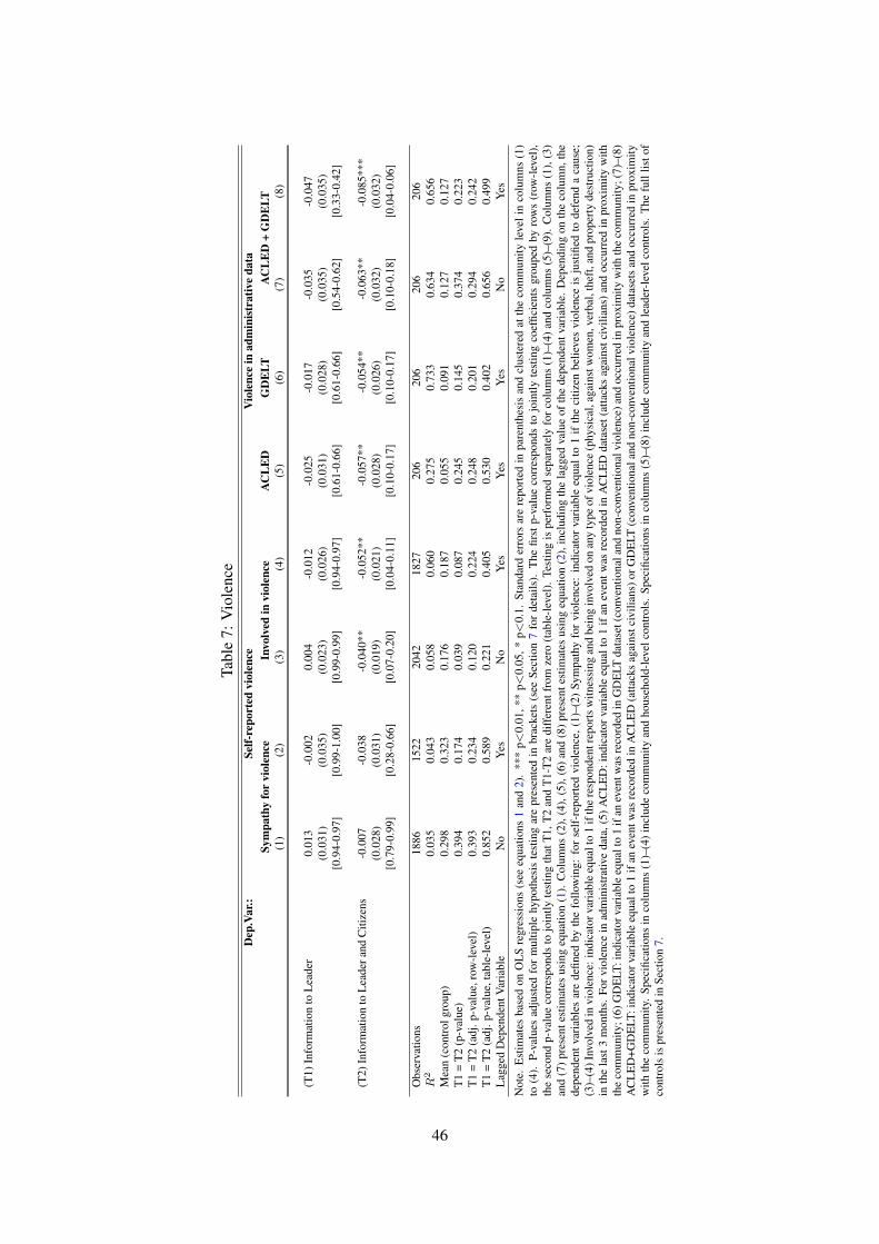
Tabl

e7:

Vio

lenc

eD

ep.V

ar.:

Self-

repo

rted

viol

ence

Vio

lenc

ein

adm

inis

trat

ive

data

Sym

path

yfo

rvi

olen

ceIn

volv

edin

viol

ence

AC

LE

DG

DE

LTA

CL

ED

+G

DE

LT(1

)(2

)(3

)(4

)(5

)(6

)(7

)(8

)

(T1)

Info

rmat

ion

toL

eade

r0.

013

-0.0

020.

004

-0.0

12-0

.025

-0.0

17-0

.035

-0.0

47(0

.031

)(0

.035

)(0

.023

)(0

.026

)(0

.031

)(0

.028

)(0

.035

)(0

.035

)[0

.94-

0.97

][0

.99-

1.00

][0

.99-

0.99

][0

.94-

0.97

][0

.61-

0.66

][0

.61-

0.66

][0

.54-

0.62

][0

.33-

0.42

]

(T2)

Info

rmat

ion

toL

eade

rand

Citi

zens

-0.0

07-0

.038

-0.0

40**

-0.0

52**

-0.0

57**

-0.0

54**

-0.0

63**

-0.0

85**

*(0

.028

)(0

.031

)(0

.019

)(0

.021

)(0

.028

)(0

.026

)(0

.032

)(0

.032

)[0

.79-

0.99

][0

.28-

0.66

][0

.07-

0.20

][0

.04-

0.11

][0

.10-

0.17

][0

.10-

0.17

][0

.10-

0.18

][0

.04-

0.06

]

Obs

erva

tions

1886

1522

2042

1827

206

206

206

206

R2

0.03

50.

043

0.05

80.

060

0.27

50.

733

0.63

40.

656

Mea

n(c

ontr

olgr

oup)

0.29

80.

323

0.17

60.

187

0.05

50.

091

0.12

70.

127

T1

=T

2(p

-val

ue)

0.39

40.

174

0.03

90.

087

0.24

50.

145

0.37

40.

223

T1

=T

2(a

dj.p

-val

ue,r

ow-l

evel

)0.

393

0.23

40.

120

0.22

40.

248

0.20

10.

294

0.24

2T

1=

T2

(adj

.p-v

alue

,tab

le-l

evel

)0.

852

0.58

90.

221

0.40

50.

530

0.40

20.

656

0.49

9L

agge

dD

epen

dent

Var

iabl

eN

oY

esN

oY

esY

esY

esN

oY

es

Not

e.E

stim

ates

base

don

OL

Sre

gres

sion

s(s

eeeq

uatio

ns1

and

2).

***

p<0.

01,*

*p<

0.05

,*p<

0.1.

Stan

dard

erro

rsar

ere

port

edin

pare

nthe

sis

and

clus

tere

dat

the

com

mun

ityle

veli

nco

lum

ns(1

)to

(4).

P-va

lues

adju

sted

for

mul

tiple

hypo

thes

iste

stin

gar

epr

esen

ted

inbr

acke

ts(s

eeSe

ctio

n7

for

deta

ils).

The

first

p-va

lue

corr

espo

nds

tojo

intly

test

ing

coef

ficie

nts

grou

ped

byro

ws

(row

-lev

el),

the

seco

ndp-

valu

eco

rres

pond

sto

join

tlyte

stin

gth

atT

1,T

2an

dT

1-T

2ar

edi

ffer

entf

rom

zero

(tab

le-l

evel

).Te

stin

gis

perf

orm

edse

para

tely

for

colu

mns

(1)–

(4)

and

colu

mns

(5)–

(9).

Col

umns

(1),

(3)

and

(7)

pres

ente

stim

ates

usin

geq

uatio

n(1

).C

olum

ns(2

),(4

),(5

),(6

)an

d(8

)pr

esen

test

imat

esus

ing

equa

tion

(2),

incl

udin

gth

ela

gged

valu

eof

the

depe

nden

tvar

iabl

e.D

epen

ding

onth

eco

lum

n,th

ede

pend

entv

aria

bles

are

defin

edby

the

follo

win

g:fo

rse

lf-r

epor

ted

viol

ence

,(1)

–(2)

Sym

path

yfo

rvi

olen

ce:

indi

cato

rva

riab

leeq

ualt

o1

ifth

eci

tizen

belie

ves

viol

ence

isju

stifi

edto

defe

nda

caus

e;(3

)–(4

)Inv

olve

din

viol

ence

:ind

icat

orva

riab

leeq

ualt

o1

ifth

ere

spon

dent

repo

rts

witn

essi

ngan

dbe

ing

invo

lved

onan

yty

peof

viol

ence

(phy

sica

l,ag

ains

twom

en,v

erba

l,th

eft,

and

prop

erty

dest

ruct

ion)

inth

ela

st3

mon

ths.

For

viol

ence

inad

min

istr

ativ

eda

ta,(

5)A

CL

ED

:ind

icat

orva

riab

leeq

ualt

o1

ifan

even

twas

reco

rded

inA

CL

ED

data

set(

atta

cks

agai

nstc

ivili

ans)

and

occu

rred

inpr

oxim

ityw

ithth

eco

mm

unity

;(6)

GD

ELT

:ind

icat

orva

riab

leeq

ualt

o1

ifan

even

twas

reco

rded

inG

DE

LTda

tase

t(co

nven

tiona

land

non-

conv

entio

nalv

iole

nce)

and

occu

rred

inpr

oxim

ityw

ithth

eco

mm

unity

;(7)

–(8)

AC

LE

D+G

DE

LT:i

ndic

ator

vari

able

equa

lto

1if

anev

entw

asre

cord

edin

AC

LE

D(a

ttack

sag

ains

tciv

ilian

s)or

GD

ELT

(con

vent

iona

land

non-

conv

entio

nalv

iole

nce)

data

sets

and

occu

rred

inpr

oxim

ityw

ithth

eco

mm

unity

.Sp

ecifi

catio

nsin

colu

mns

(1)–

(4)

incl

ude

com

mun

ityan

dho

useh

old-

leve

lcon

trol

s.Sp

ecifi

catio

nsin

colu

mns

(5)–

(8)

incl

ude

com

mun

ityan

dle

ader

-lev

elco

ntro

ls.

The

full

listo

fco

ntro

lsis

pres

ente

din

Sect

ion

7.

46

Table 8: DeliberationInformation only Information plus deliberation

Outcome variable Mean Coeff. S.E. N(1) (2) (3) (4)

Community-level outcomesLeader’s knowledge 0.439 -0.006 0.089 101Leader’s perceived benefits 0.070 -0.163 0.209 101Elite capture -0.020 0.049 0.072 100Rent-seeking among leaders 0.029 0.093 0.153 100Violence -0.150 -0.059 0.098 101

Citizen-level outcomesCitizen’s knowledge 0.482 0.006 0.036 1014Citizen’s perceived benefits 0.163 -0.013 0.057 893Rent-seeking among citizens 0.028 -0.008 0.031 989Citizen’s mobilization 0.032 0.131* 0.067 830Trust and accountability 0.083 -0.061* 0.032 777Self-reported violence -0.068 0.010 0.040 910

Note. Estimates based on OLS regressions (see equation 1). *** p<0.01, ** p<0.05, * p<0.1. Standard errors are reported in column(3) and clustered at community level when employing citizen-level outcomes. The specifications include community and household-level controls (for citizen-level outcomes) or community-level controls (for community-level outcomes). The full list of controls ispresented in Section 7. Outcomes are grouped in indices that are built using the Kling et al. (2007) procedure. Outcomes are firstnormalized in standardized units to study mean effect sizes of the indices relative to the standard deviation of the control group andthen averaged within each category.

47

ONLINE APPENDIX FOR“DOES INFORMATION BREAK THE POLITICAL RESOURCE CURSE?”

A Information module

The information module is based on a detailed information manual. Presentations to the commu-

nities, based on the manual, are composed of the following parts:

1. Presentation. This is an introductory space for those holding the meetings in the communities

to present themselves and the implementing partners, and to introduce the subject of the meet-

ing. This is also a moment for the community leader or any other influential person to explain

to the community the contents and objectives of the meeting.

2. Introduction. Presenters explain that Mozambique is endowed with many different types of

natural resources in large quantities, with the extractive industries of natural gas, coal, iron,

precious stones and heavy minerals are in rapid expansion. The extractive industries offer

potential for investment and creation of wealth. The first mention of the importance of the

natural gas reserves discovered in the Rovuma Basin happens at this point. Specifically, it is

explained that, according to the IMF, during the 2020s, the natural gas industry will account for

half of the country’s wealth.2 This discovery has the potential to place Mozambique in the top

producers of natural gas worldwide and the future of its economy may be heavily influenced

by the management of the revenues generated by the extraction.

3. Natural resources. Presenters discuss the formal definition of a natural resource, and the

difference between renewable and non-renewable resources. This distinction is important for

the communities to understand that many of their resources are non-renewable, and therefore

sustainability is an issue. Resources should generate benefits for present and future generations

in an equitable way. Hence, environmental considerations should be taken into account. Then

presenters cover the types of natural resources relevant for Cabo Delgado, i.e., minerals, forest

resources, fishing, and natural gas.

4. Natural gas. Presenters provides detailed information about the natural gas discovery, in-

cluding where in Cabo Delgado it was discovered, and the plans over the next few years for

the exploration and transformation of natural gas. A brief mention of the uses of natural gas

follows. At the end, presenters mention that Inhambane, another province in Mozambique,

discovered natural gas in the past and what lessons were learned from that experience.2International Monetary Fund (IMF), Country Report No. 16/10 (January, 2016).

1

5. The importance for citizens. This part shed light on what the local population can expect from

the exploration of natural resources. Presenters explain that natural resources can be a source of

income for the families, either through governmental transfers or through the creation of jobs,

and that extractive companies operating locally should be aware of their social responsibility

towards the citizens.

6. Examples. At this point, presenters discuss three examples of countries that discovered natural

resources, including how they impacted their populations. Two examples are positive (Nor-

way and Botswana), and one is negative (Nigeria). These cases exemplify both desirable and

undesirable consequences from the discovery of natural resources.

7. Conclusion. The meeting is concluded with a brief review of the topics covered, emphasizing

the main lessons. Although citizens are allowed to raise questions during the meeting, this is

typically the moment when most participants express their opinion.

B Sampling and randomization: further details

The 206 communities in the final sample were randomly drawn from the sampling frame of 421

polling stations. To obtain the sampling frame, 54 polling stations that were not operating in

both the 2009 and 2014 general elections were excluded. Additionally, the smallest 5th percentile

by voter size (corresponding to a cutoff of 207 voters) was also excluded. The polling locations

were located within the following 16 districts in Cabo Delgado: Ancuabe, Balama, Chiure, Ma-

comia, Mecufi, Meluco, Metuge, Mocimboa da Praia, Montepuez, Mueda, Muidumbe, Namuno,

Nangade, Palma, Pemba, and Quissanga. The Ibo district was excluded since it is an island, to-

gether with two other polling stations in another island. Eleven polling stations in Palma’s “posto

administrativo” were also excluded to avoid areas that experienced recent violent events.

Sampled communities were stratified by the two urban areas (Pemba and Montepuez), semi-urban

communities (i.e., the main “posto administrativo” in each district) and rural communities. In

urban strata, 8 polling locations were selected in Pemba and 4 in Montepuez; in semi-urban strata,

2 polling stations were selected per town (1 if only 1 was available); the remaining 165 stations

were sampled from all other polling stations. To secure representation of the few urban settlements

in the province, sampling embeds an oversampling of urban and semi-urban locations. Figure

B1 presents a comparison of the distribution of registered voters in the sampling frame and the

sampled locations. Figure B2 presents the distribution among different districts of the number of

polling locations and the number of sampled polling locations. The stratified random sampling

tends to replicate the distribution of polling stations in the sampling frame.

2

Figure B1: Distribution of voters in sampled polling locations versus all locations

0

.0001

.0002

.0003

.0004

.0005

Den

sity

0 2000 4000 6000 8000 10000Number of voters per polling station

All polling stations Sampled polling stations

Note. The blue line presents the distribution of the number of registered voters per polling location in the sampling frame, whilethe red line presents the same distribution in the sampled polling locations.

Before implementing the randomization procedure, blocks of four communities were built imple-

menting a code using Mahalanobis-distance and making use of the richness of baseline informa-

tion. The following variables were used to compute the metric:

• Household characteristics. For each community, the mean household was constructed averag-

ing the gender, age, education and income of the respondents, their household size, the share

of Muslim households, the share of households from different ethnic groups (Macua, Maconde,

Mwani), an asset index averaging ownership of all different assets and a self-reported violence

index (built using information on whether the respondent observed or has been affected by vi-

olent events). Additional controls include average trust in the community, share of respondents

who know an influential person, a religious leader or a community leader, share of respondents

participating in organizations, the average attitudes towards bribes and towards the allocation

of public funds, the share of respondents born in the village, the share of respondents earning

money, and the share looking for a job.

• Leader and Community characteristics. Variables included are gender, age, education of the

community leader, his/her trust, his/her knowledge of influential people, his/her attitudes to-

wards bribes and towards the allocation of public funds, whether he/she is Muslim, and whether

he/she is active as member of an organization. Community characteristics are measured by two

indices averaging binary variables, one on the quality of infrastructures and one on the presence

of natural resources.

Sampling of citizens within communities was the product of physical random walks during the

baseline survey. Enumerators were told to select houses by departing in different directions from

the center of the community as defined by the polling location. They were given a sampling

interval for each community, which was a function of the number of registered voters in that

3

Figure B2: Geographic distribution of polling locations and sampled polling locationsAll stations Sample

No station 1-25 stations26-50 stations 51-100 stations101-150 stations 151+ stations

No station 1-10 stations11-20 stations 21-30 stations31-40 stations 41-50 stations51+ stations

Note. The left panel presents the geographic distribution of the number of polling locations. The right panel shows the sameinformation, but restricted to sampled polling locations. In maps, Metuge is included in Pemba district and Ibo is included inQuissanga district.

community. The sampling interval defined the number of houses in between sampled houses.

B.1 Attrition and sample selection

This section analyzes attrition at the follow-up household survey. Columns (1)–(2) in Table B1

present probit regressions of household-level attrition under different specifications. The depen-

dent variable is equal to 1 if the household was interviewed at baseline and not re-interviewed

at follow-up, and zero if the household was interviewed in both rounds. Columns (3)–(4) check

whether the refresher sample at follow-up was added differentially in different treatment arms.

The dependent variable is a dummy variable equal to 1 if, at follow-up, the observation is from the

refresher sample and zero if it is from the baseline.

Table B1: Attrition and sample selection at follow-upDep.var.: Attrition from baseline to follow-up Refresher sample at follow-up

(1) (2) (3) (4)(T1) Information to Leader (d) 0.014 0.018 -0.015 -0.010

(0.018) (0.019) (0.017) (0.017)(T2) Information to Leader and Citizens (d) -0.010 -0.010 -0.022 -0.022

(0.015) (0.014) (0.014) (0.014)Observations 2065 2065 2103 2103Mean (control group) 0.083 0.083 0.114 0.114Randomization Strata No Yes No Yes

Note. Estimates based on probit regressions (marginal effects). *** p<0.01, ** p<0.05, * p<0.1. Standard errors are reported inparenthesis and clustered at the community level. Depending on the column, the dependent variables are defined by the following:(1)–(2) Attrition from baseline to follow-up: dummy variable equal to 1 if the household was interviewed at baseline and not re-interviewed at follow-up, and zero if the household was interviewed in both rounds; (3)–(4) Refresher sample at follow-up: dummyvariable equal to 1 if, at follow-up, the observation is from the refresher sample and zero if it is from the baseline.

4

B.2 Balance checks

Table B2 presents randomization checks for respondent, leader, and community characteristics.

For each outcome of household/leader i living in community j, Yij , balance is first tested using

the following least squares regression:

Yij = α+ β Tj + εij (4)

where Tj is an indicator variable for living in a community in either treatment 1 or treatment 2. εijis an individual-specific error term clustered at the community level for household-level outcomes.

A second specification is also estimated:

Yij = α+ β1 T1j + β2A T2Aj + β2B T2Bj + εij (5)

where T1j , T2Aj and T2Bj are indicator variables for living in a community in treatment groups

1, 2A (information to leader and citizens without deliberation), and 2B (information to leader and

citizens plus deliberation). εij is an individual-specific error term clustered at the community level.

A test for joint-significance of β1, β2A and β2B using an F-test is also provided.

5

Table B2: Descriptive StatisticsTreatment Group:

Control Any T1 T2A T2B Joint test(1) (2) (3) (4) (5) (6)

mean diff. diff. diff. diff. p-value[std.dev.] (std.err.) (std.err.) (std.err.) (std.err.) [N]

Citizen-levelFemale 0.274 -0.033 -0.036 -0.037 -0.026 0.668

[0.446] (0.027) (0.034) (0.036) (0.034) [2065]Age in years 44.880 0.220 0.280 0.655 -0.285 0.884

[16.860] (1.010) (1.296) (1.255) (1.178) [2058]Household size 5.588 0.102 -0.098 0.208 0.193 0.329

[2.861] (0.168) (0.198) (0.214) (0.198) [2063]No formal education 0.310 -0.020 -0.022 -0.017 -0.022 0.889

[0.463] (0.027) (0.032) (0.033) (0.034) [2065]Primary education 0.575 0.002 0.025 0.010 -0.029 0.516

[0.495] (0.030) (0.036) (0.037) (0.037) [2065]Secondary or higher education 0.114 0.018 -0.002 0.006 0.052 0.423

[0.319] (0.024) (0.027) (0.027) (0.035) [2065]Years of schooling 3.690 0.077 0.004 -0.102 0.334 0.564

[3.405] (0.237) (0.274) (0.270) (0.325) [2065]Muslim 0.555 0.017 0.015 0.044 -0.007 0.897

[0.497] (0.060) (0.075) (0.073) (0.072) [2065]Macua ethnic group 0.599 0.049 0.083 0.031 0.033 0.784

[0.491] (0.065) (0.081) (0.081) (0.083) [2065]Maconde ethnic group 0.294 -0.045 -0.054 -0.061 -0.020 0.839

[0.456] (0.063) (0.078) (0.075) (0.078) [2065]Mwani and other ethnic groups 0.107 -0.004 -0.029 0.029 -0.013 0.556

[0.309] (0.032) (0.035) (0.044) (0.038) [2065]Semi-urban 0.109 -0.005 -0.009 -0.001 -0.003 0.999

[0.313] (0.049) (0.060) (0.062) (0.061) [1950]Urban 0.091 -0.035 -0.031 -0.037 -0.037 0.878

[0.288] (0.043) (0.052) (0.050) (0.051) [1950]Average Trust 2.177 -0.016 -0.034 -0.045 0.032 0.297

[0.546] (0.037) (0.044) (0.046) (0.045) [1949]Awareness of natural gas discovery 0.487 0.002 -0.053 0.026 0.033 0.381

[0.500] (0.047) (0.056) (0.055) (0.058) [2064]Listens to radio frequently 0.394 0.017 -0.017 0.039 0.028 0.362

[0.489] (0.028) (0.034) (0.035) (0.036) [2063]

Community-levelFemale Leader 0.036 -0.016 -0.036 0.003 -0.016 0.556

[0.189] (0.024) (0.030) (0.030) (0.030) [206]Leader’s age 54.091 0.505 0.549 0.517 0.449 0.991

[10.624] (1.556) (1.940) (1.930) (1.940) [206]Years of schooling 6.200 -0.783* -0.500 -0.631 -1.220** 0.182

[2.946] (0.446) (0.554) (0.551) (0.554) [206]Natural resources index 0.044 -0.001 -0.014 0.013 -0.004 0.180

[0.060] (0.010) (0.012) (0.012) (0.012) [206]Infrastructure index 0.483 0.014 -0.000 0.032 0.011 0.702

[0.150] (0.025) (0.031) (0.031) (0.031) [206]

Note. *** p<0.01, ** p<0.05, * p<0.1. Column (1) reports sample mean and standard deviation in brackets for the control group.Column (2) reports the difference between all treatment groups pooled together and the control group using an OLS regression ofthe corresponding characteristic on the treatment indicator. Columns (3)–(5) report the difference between each treatment group andthe control group. Standard errors clustered at community level are reported in parentheses. Column (5) presents a joint test ofsignificance of the coefficients for each treatment dummy (columns 3 to 5). Average Trust is the average of all self-reported measuresof trust and ranges from 0 = not at all to 3 = trust a lot. Natural Resources index is built averaging 10 dummy variables indicating thepresence in the community of different natural resources (limestone, marble, sands, forest, ebony, exwood, gold, charcoal, graphite,semi-precious and precious stones, mercury, fishing resources, salt and natural gas). Infrastructure index is built averaging 14 dummyvariables indicating the presence in the community of a kindergarten, a primary school, a lower secondary school, an high school, anhealth center, a facilitator, a water pump, a market, a police station, a religious building, an amusement area, a room for communityactivities, access to electricity and connection to sewage.

6

C Multiple hypothesis testing procedure

For multiple hypothesis testing, the Studentized k-StepM method for the two-sided setup (Romano

and Wolf, 2005) is followed. Data is represented by a data matrix XN , where N is the number

of observations generated from some underlying unknown probability mechanism P . Interest

focuses on the parameter vector θ = (θT1 θT2)′, where each θt = (βt,1, ..., βt,K), and βt,k is the

parameter on the treatment vector t = (T1 T2)′ corresponding to equations (1) and (2) estimated

with outcome variable k. Individual hypotheses concern all elements of θ, and are two-sided:

Ht,k : βt,k = 0 vs H′t,k : βt,k 6= 0. For each element of θ, the test of the difference between

treatment effects is analogously considered. For a given set of hypotheses, the following procedure

is implemented:

1. Let θN denote an estimator of θ (with std. errors σN,t,k) computed from the original data

matrix XN using specifications presented in Section 7. For each hypothesis Ht,k, the abso-

lute studentized test statistics |zN,t,k| =∣∣∣βN,t,k/σN,t,k

∣∣∣ is computed from the data matrix

XN and relabeled in descending order from r1 to rS , such that zN,r1 ≥ zN,r2 ≥ ... ≥ zN,rS .

2. Generate M bootstrap data matrices X∗,mN with 1 ≤ m ≤M (M is set at 2000). Due to the

design of the experiment, bootstrap data matrices are clustered at the community level. From

each bootstrap data matrix, estimates β∗,mN,t,1, ..., β∗,mN,t,K and standard errors σ∗,mN,t,1, ..., σ

∗,mN,t,K

are computed using the same specifications as in Step 1. Then set j = 1 and R0 = 0.

3. For 1 ≤ m ≤ M , compute max∗,mN,j = maxRj−1+1≤s≤S

(∣∣∣β∗,mN,rs− βN,rs

∣∣∣ /σ∗,mN,rs

). Using

the M max∗,mN,j , compute dj as the 1 − α empirical quantile of the M values max∗,mN,j . For

Rj−1 + 1 ≤ s ≤ S, if |zN,rs | > dj , reject the null hypothesis Hrs . α is set at 10%.

4. If no further hypotheses are rejected, the procedure stops. Otherwise, denote by Rj the

number of hypotheses rejected so far, let j = j + 1 and return to Step 3.

To compute p-values, we follow the procedure for the computation of p-values adjusted for step-

down multiple testing (see Algorithm 4.1 in Romano and Wolf, 2016).

D Additional Analysis

D.1 Knowledge of the natural gas discovery

An index is built from the following 5 questions: “Where was natural gas discovered?”, “Do you

think that the exploration of natural gas has begun?”, “Do you think that the government has al-

ready started receiving revenues from natural gas?”, “What year do you think the extraction of

7

natural gas will begin?”, and “What are the names of the companies involved in the exploration of

natural gas?”. Table D3 reports estimates of treatment effects on whether the respondent knows

the correct answer for each of these questions. Each indicator variable is equal to 1 if the re-

spondent provides a correct answer, and 0 otherwise. Answers to each individual questions are

averaged into an index, equal to 1 if the respondent has full knowledge of the discovery and zero

if the respondent reports all answers wrongly or has never heard about the discovery. The open-

ended nature of these questions is exploited, allowing the construction of 15 indicator variables

capturing whether the respondent provides an answer and whether it is correct. The value 1 is

assigned if the respondent reports correct information and does not report wrong information, and

0 if the respondent reports wrong information or does not know the answer. The 15 indicators are

then averaged into a single index.

Table D3: Knowledge of the natural gas discovery(T1) (T2)

Information to Leader Information to Leader F-testand Citizens equality

Outcome variable Coeff. S.E. Coeff. S.E. (p-value) N(1) (2) (3) (4) (5) (6)

Leaders’ knowledgeKnows the location of discovery 0.019 0.047 0.093** 0.042 0.058 206Knows whether exploration started 0.158** 0.069 0.160** 0.062 0.023 206Knows whether government receives revenues 0.027 0.082 -0.017 0.074 0.836 206Knows expected start of extraction 0.074 0.084 0.162** 0.075 0.095 206Knows companies involved 0.022 0.014 0.024* 0.013 0.150 206

Citizens’ knowledgeKnows the location of discovery 0.025 0.026 0.237*** 0.022 0.000 2072Knows whether exploration started -0.017 0.034 0.242*** 0.028 0.000 2072Knows whether government receives revenues -0.044* 0.026 0.086*** 0.024 0.000 2072Knows expected start of extraction 0.024 0.020 0.175*** 0.021 0.000 2072Knows companies involved -0.008 0.021 0.154*** 0.016 0.000 2072

Note. Estimates based on OLS regressions (see equation 1). *** p<0.01, ** p<0.05, * p<0.1. Standard errors are reported in columns(2) and (4) and clustered at the community level. Each variable ranges from 0 to 1, where 0 indicates zero knowledge, and 1 indicatesfull knowledge. The specification includes community and leader-level controls (leaders), or community and household-level controls(citizens). The full list of controls is presented in Section 7.

Table D4 presents the main correlates of awareness and knowledge by citizens about the natural

gas discovery at baseline. Columns 1 and 3 include only household-level controls, while columns

2 and 4 include community and leader-level controls in addition to the household-level controls.

Individual characteristics are the main determinants of citizen awareness and knowledge at the

baseline.

8

Table D4: Correlates of awareness and knowledge at baselineDep.Var. Awareness Knowledge

(1) (2) (3) (4)Female respondent -0.195*** -0.213*** -0.134*** -0.152***

(0.026) (0.025) (0.017) (0.016)Age in years 0.014*** 0.014*** 0.011*** 0.010***

(0.004) (0.003) (0.002) (0.002)Age (squared) -0.000*** -0.000*** -0.000*** -0.000***

(0.000) (0.000) (0.000) (0.000)Primary education 0.099*** 0.111*** 0.072*** 0.078***

(0.022) (0.021) (0.015) (0.014)Secondary or higher education 0.408*** 0.362*** 0.301*** 0.254***

(0.037) (0.038) (0.026) (0.025)Muslim 0.140*** 0.065*** 0.096*** 0.031*

(0.025) (0.024) (0.017) (0.016)Macua ethnic group -0.289*** -0.074* -0.229*** -0.058**

(0.038) (0.038) (0.031) (0.027)Maconde ethnic group 0.149*** -0.117** 0.055 -0.084**

(0.047) (0.049) (0.035) (0.034)Household size 0.015*** 0.012*** 0.010*** 0.008***

(0.003) (0.003) (0.002) (0.002)Born in the village 0.022 0.025 0.018 0.023*

(0.021) (0.020) (0.015) (0.014)In monogamous marriage -0.035 -0.020 -0.036** -0.022

(0.022) (0.021) (0.015) (0.014)Subsistence farmer -0.065*** -0.055** -0.043*** -0.032**

(0.022) (0.022) (0.016) (0.015)Infrastructure index -0.008 -0.033

(0.097) (0.073)Natural resources index -0.258 -0.206

(0.191) (0.133)Number of voters 0.001 0.003

(0.008) (0.006)Below median distance from Palma 0.225*** 0.177***

(0.044) (0.031)Share of community of Macua ethnic group -0.116 -0.120**

(0.071) (0.059)Share of community of Maconde ethnic group 0.240*** 0.068

(0.076) (0.061)Share of community with secondary or higher education 0.106 0.087

(0.080) (0.055)Observations 2055 2055 2055 2055R2 0.229 0.301 0.248 0.341District indicator variables No Yes No YesStratum indicator variables No Yes No Yes

Note. Estimates based on OLS regressions (see equations 1 and 2). *** p<0.01, ** p<0.05, * p<0.1. Standard errors are reportedin parenthesis and clustered at the community level. Depending on the column, the dependent variables are defined by the following:(1)–(2) Awareness: indicator variable equal to 1 if the respondent reports having heard about the natural gas discovery; (3)–(4)Knowledge: index averaging 15 indicator variables related to knowledge about the location of the discovery, whether exploration hasstarted, whether the government is receiving revenues, when extraction is expected to start, and which firms are involved. Stratumindicator variables include dummy variables for semi-urban and urban strata (excluded category is rural stratum). Number of voters ismeasured as the number of tables at the polling station. The full list of controls is presented in Section 7.

9

D.2 Information spillovers and the evolution of the control group

The sample is split in communities close to (or far from) another community in T1 and in com-

munities close to (or far from) another community in T2. Being close to or far from are defined

using the sample median of the minimum distance to another community of these types. These

median minimum distances are 12.01 km to T1 and 9.65 km to T2. The effect of each treatment

is then estimated for each sub-group. Figure D3 presents the results relating to the effect of the

interventions on leader’s knowledge and salience of the natural gas discovery (upper panels), and

on citizen’s knowledge and salience of the natural gas discovery (lower panels). No evidence is

found of spillover effects since estimates are not statistically different across sub-groups.3

Figure D3: Spillover effects on knowledge and salience about the natural gas discovery

-0.05

0.00

0.05

0.10

0.15

Aver

age

Trea

tmen

t Effe

ct

T1 T2

Leaders' knowledge

-0.20

0.00

0.20

0.40

0.60

Aver

age

Trea

tmen

t Effe

ct

T1 T2

Leaders' salience

-0.10

0.00

0.10

0.20

0.30

Aver

age

Trea

tmen

t Effe

ct

T1 T2

Citizens' knowledge

-0.10

0.00

0.10

0.20

0.30

0.40

Aver

age

Trea

tmen

t Effe

ct

T1 T2

Citizens' salience

Close to T2 Far from T2 Close to T1 Far from T1

Note. Close to and Far from are based on the sample median of the minimum distance of a community to another community in T1 andin T2. The sample is split in communities closer than the median minimum distance (close to) and further away (far from). Minimummedian distances are 12.01 km to T1 and 9.65 km to T2. Estimates based on OLS regression (see equations 1). Confidence intervalsare built using statistical significance at the 10% level. Standard errors are clustered at the community level. For leader’s knowledgeand salience, the specifications include community and leader-level controls. For citizen’s knowledge and salience, the specificationsinclude community and household-level controls. The full list of controls is presented in Section 7.

Figure D4 shows the evolution between baseline and endline surveys of average awareness, knowl-

edge, and salience of the natural gas discovery in the control group. The left panel focuses on

leaders, while the right panel focuses on citizens. While leaders are much more aware of the dis-

covery when compared to citizens, awareness increases over time for both. This is particularly

the case among citizens. For citizens, a similar trend is observed for knowledge and salience.3A similar conclusion is achieved when looking at awareness of the natural gas discovery. Estimates are omitted

since in communities close to T2 all leaders are aware of the discovery. Therefore the treatment effect cannot beestimated for that group.

10

For leaders, knowledge tends to remain constant, while salience is slightly reduced. Since no

contamination across communities is observed, this pattern suggests that, in the absence of any

information campaign, news about the discovery reach citizens through alternative sources.

Figure D4: Evolution of awareness, knowledge, and salience in the control group

Note. The figure shows average awareness, knowledge, and salience of the natural gas discovery at baseline and follow-uprestricted to the control group. The left panel focuses on leaders, while the right panel focuses on citizens.

D.3 Interaction with local leaders

Figure D5 shows the relative importance of different categories in the networks of leaders and

citizens. Individuals in these networks are grouped into four major categories: local chiefs, other

political leaders, public administration, religious community and other influential people. Local

chiefs includes the village chief, his deputy and the chiefs for sub-units of the community. Other

political leaders includes all higher level politicians (such as district and province-level govern-

ments), members of the party, the members of the community council, and all traditional leaders.

Public administration includes all individuals working in the public administration. Religious

community includes all religious leaders (imams and priests) and religious teachers. Other influ-

ential people is a residual category.

To understand interactions within the network, the left panel in Figure D6 shows whether citizens

talked or called any of these individuals in the 6 months previous to the interview. The right

panel in figure D6 analyzes instead the average trust towards these individuals. Figure D7 presents

estimates of the effect of the interventions on the interaction of the leader and the citizens with

people in their corresponding networks, both employing extensive (left panels) and intensive (right

panels) margins. Results are similar across the two margins, and are suggestive that, consistently

with figure D6, the interventions lead to different patterns of interaction with local leaders when

comparing leaders to citizens.

11

Figure D5: Interaction with leaders

0 .1 .2 .3 .4 .5Share of overall network

Public Administration

Local chiefs

Other influential people

Religious community

Other political leaders

Leaders

0 .1 .2 .3 .4Share of overall network

Public Administration

Local chiefs

Other influential people

Other political leaders

Religious community

Citizens

Note. The figure presents the composition at baseline of the network of all respondents (leaders in the left panel and citizens in theright panel). Categories are ordered from top to bottom in terms of relative importance within the network.

Figure D6: Network and interaction with local leaders

0

.2

.4

.6

.8

1

Shar

e in

tera

ctin

g wi

th

Leader

0

.2

.4

.6

.8

1

Shar

e in

tera

ctin

g wi

th

Citizens

Interaction with leaders

Local chiefs Other political leadersPublic administration Religious community and other influential people

2.5

2.75

3

Aver

age

trust

(0-4

)

Leader

2.5

2.75

3

Aver

age

trust

(0-4

)

Citizens

Trust for leaders

Local chiefs Other political leadersPublic administration Religious community and other influential people

Note. The left figure shows the share of respondents that interacted with leaders in the corresponding category (for leaders andcitizens). Interaction is defined as whether the respondent reports having called or talked with a leader in the 6 months previous to theinterview. The right figure presents average trust for known leaders reported by both leaders and citizens. Trust is self-reported (0 =not at all to 3 = trust a lot). The sample is restricted to the baseline survey.

Figure D7: Interaction with leaders and the effect of the interventions

-.3

-.2

-.1

0

.1

.2

.3

T1 T2

Leader's interaction

-.3

-.2

-.1

0

.1

.2

.3

T1 T2

Citizen's interaction

Local chiefs Other political leadersPublic administration Religious community and other influential people

-1.5

-1

-.5

0

.5

1

T1 T2

Leader's log-interactions

-.4

-.2

0

.2

.4

.6

T1 T2

Citizen's log-interactions

Local chiefs Other political leadersPublic administration Religious community and other influential people

Note. Estimates based on OLS regressions (see equation 1). Confidence intervals are built using statistical significance at the 10%level, and standard errors clustered at the community level when employing citizen-level outcomes. In the left panels, the dependentvariable is an indicator variable equal to 1 if the respondent reports having talked or called a leader in the corresponding category in the6 months previous to the interview. In the right panels, the dependent variable is the log total number of times the respondent interactedwith leaders in the corresponding category. The specifications include community and leader-level controls (for leader-level outcomes)or community-level and household-level controls (for citizen-level outcomes). The full list of controls is presented in Section 7.

12

D.4 Heterogeneous effects

This section presents an analysis of heterogeneous effects by basic demographics of the citizens

(table D5), by baseline social capital (table D6), and by baseline wealth, awareness, aspirations,

and risk/patience attitudes (table D7). Categories are identified in the pre-analysis plan (Armand

et al., 2017). Outcomes are grouped in indices that are built using the procedure followed by Kling

et al. (2007).

Table D5: Heterogeneous effects: basic demographics of citizensT1 T2 T1 T2

Outcome variable Coeff. S.E. Coeff. S.E. N Coeff. S.E. Coeff. S.E. N(1) (2) (3) (4) (5) (6) (7) (8) (9) (10)

Below median distance from Palma Above median distance from PalmaCitizen-level outcomesCitizen’s knowledge 0.01 0.06 0.29*** 0.06 1001 0.06 0.08 0.78*** 0.06 1071Rent-seeking among citizens 0.17*** 0.05 0.13*** 0.04 975 0.03 0.05 -0.03 0.04 1052Citizen’s mobilization 0.05 0.08 0.09 0.07 866 0.10 0.08 0.19** 0.09 835Trust and accountability 0.04 0.04 0.07* 0.04 686 -0.03 0.05 0.07 0.04 883Self-reported violence 0.03 0.07 -0.00 0.05 931 0.04 0.07 -0.11* 0.06 924

Community-level outcomesLeader’s knowledge -0.01 0.10 0.03 0.10 100 0.47*** 0.17 0.97*** 0.15 106Leader’s perceived benefits 0.07 0.23 0.04 0.22 100 0.09 0.30 -0.19 0.28 104Elite capture 0.13* 0.08 0.04 0.07 99 0.19* 0.10 -0.09 0.09 106Rent-seeking among leaders 0.11 0.16 0.24 0.15 99 -0.12 0.19 -0.16 0.17 105Violence -0.25 0.17 -0.40** 0.16 100 -0.04 0.07 -0.04 0.07 106

Younger citizens (< 35 y.o.) Older citizens (≥ 35 y.o.)Citizen-level outcomesCitizen’s knowledge -0.10 0.09 0.52*** 0.07 555 0.08 0.06 0.55*** 0.05 1517Rent-seeking among citizens 0.13** 0.06 0.03 0.04 541 0.11** 0.04 0.06* 0.04 1486Citizen’s mobilization 0.08 0.07 0.12* 0.06 462 0.05 0.06 0.13** 0.06 1239Trust and accountability -0.05 0.06 0.05 0.05 431 -0.01 0.04 0.05 0.03 1138Self-reported violence -0.12 0.10 -0.16** 0.07 502 0.11** 0.05 0.01 0.05 1353

Less educated (≤ 4 years of schooling) More educated (> 4 years of schooling)Citizen-level outcomesCitizen’s knowledge 0.06 0.07 0.60*** 0.05 1269 -0.03 0.09 0.44*** 0.07 803Rent-seeking among citizens 0.11** 0.05 0.08** 0.04 1242 0.10** 0.05 0.01 0.04 785Citizen’s mobilization 0.07 0.06 0.14** 0.06 1069 0.04 0.07 0.13** 0.06 632Trust and accountability -0.03 0.04 0.03 0.03 919 -0.00 0.05 0.07* 0.04 650Self-reported violence 0.04 0.05 -0.03 0.05 1123 0.05 0.09 -0.07 0.06 732

Female citizen Male citizenCitizen-level outcomesCitizen’s knowledge -0.03 0.09 0.50*** 0.08 584 0.07 0.07 0.58*** 0.05 1488Rent-seeking among citizens 0.12* 0.06 0.11** 0.05 574 0.12*** 0.04 0.03 0.04 1453Citizen’s mobilization 0.13 0.08 0.20*** 0.07 471 0.05 0.06 0.12** 0.06 1230Trust and accountability -0.07 0.06 0.03 0.05 424 0.00 0.03 0.07** 0.03 1145Self-reported violence 0.08 0.11 -0.01 0.07 511 0.05 0.06 -0.06 0.05 1344

Note. Estimates based on OLS regression (see equation 1). *** p<0.01, ** p<0.05, * p<0.1. Standard errors are reported in columns(2), (4), (7), and (9) and clustered at the community level for citizen-level outcome variables. The specifications include communityand leader-level controls (for leader-level outcomes) or community-level and household-level controls (for citizen-level outcomes).The full list of controls is presented in Section 7. Outcomes are grouped in indices that are built using the procedure followed byKling et al. (2007): outcomes are first normalized in standardized units to study mean effect sizes of the indices relative to the standarddeviation of the control group and then averaged within each category.

13

Table D6: Heterogeneous effects: baseline social capitalT1 T2 T1 T2

Outcome variable Coeff. S.E. Coeff. S.E. N Coeff. S.E. Coeff. S.E. N(1) (2) (3) (4) (5) (6) (7) (8) (9) (10)

Does not know chiefs Knows chiefsCitizen-level outcomesCitizen’s knowledge -0.06 0.09 0.46*** 0.07 737 0.09 0.07 0.61*** 0.05 1335Rent-seeking among citizens 0.10* 0.06 0.06 0.04 721 0.08* 0.04 0.07* 0.04 1306Citizen’s mobilization 0.11* 0.06 0.25*** 0.06 597 0.05 0.07 0.10 0.07 1104Trust and accountability -0.03 0.07 -0.05 0.06 460 -0.01 0.04 0.10*** 0.03 1109Self-reported violence 0.02 0.08 -0.04 0.06 633 0.04 0.07 -0.05 0.05 1222

Does not know other political leaders Knows other political leadersCitizen-level outcomesCitizen’s knowledge 0.03 0.08 0.52*** 0.07 886 0.06 0.07 0.61*** 0.05 1186Rent-seeking among citizens 0.14*** 0.04 0.06 0.04 874 0.10** 0.04 0.05 0.04 1153Citizen’s mobilization 0.08 0.06 0.20*** 0.05 736 0.06 0.08 0.08 0.07 965Trust and accountability -0.02 0.05 0.09* 0.05 582 -0.01 0.05 0.04 0.04 987Self-reported violence 0.06 0.07 -0.04 0.06 784 0.03 0.07 -0.05 0.06 1071

Leader is less network-central Leader is more network-centralCitizen-level outcomesCitizen’s knowledge 0.00 0.08 0.65*** 0.06 1178 -0.04 0.08 0.28*** 0.09 708Rent-seeking among citizens 0.05 0.05 0.04 0.04 1156 0.15** 0.06 0.03 0.06 693Citizen’s mobilization 0.13 0.08 0.21*** 0.08 987 -0.04 0.09 -0.00 0.08 567Trust and accountability -0.01 0.05 0.07* 0.04 890 -0.04 0.04 0.03 0.05 536Self-reported violence 0.04 0.09 -0.10* 0.06 1032 -0.01 0.06 -0.03 0.06 659

Community is less mobilized Community is more mobilizedCitizen-level outcomesCitizen’s knowledge 0.04 0.07 0.53*** 0.05 1341 -0.06 0.11 0.53*** 0.08 731Rent-seeking among citizens 0.13*** 0.05 0.04 0.04 1309 0.04 0.06 0.06 0.04 718Citizen’s mobilization 0.14** 0.07 0.16** 0.07 1074 0.05 0.12 0.06 0.10 627Trust and accountability -0.03 0.04 0.06 0.04 1021 0.03 0.05 0.07* 0.04 548Self-reported violence 0.10* 0.05 -0.02 0.04 1193 -0.12 0.09 -0.07 0.07 662

Lower voice outside the community Higher voice outside the communityCitizen-level outcomesCitizen’s knowledge 0.07 0.08 0.56*** 0.07 1059 -0.01 0.07 0.55*** 0.06 1013Rent-seeking among citizens 0.02 0.05 -0.03 0.05 1032 0.19*** 0.05 0.15*** 0.04 995Citizen’s mobilization -0.00 0.08 0.03 0.07 868 0.16** 0.08 0.23*** 0.09 833Trust and accountability -0.01 0.04 0.06* 0.03 782 -0.03 0.05 0.07 0.05 787Self-reported violence 0.08 0.06 0.05 0.05 980 0.03 0.07 -0.15** 0.06 875

Lower trust Higher trustCitizen-level outcomesCitizen’s knowledge 0.02 0.07 0.46*** 0.06 1012 0.09 0.09 0.68*** 0.07 1060Rent-seeking among citizens 0.11* 0.05 0.05 0.05 989 0.10* 0.06 0.03 0.04 1038Citizen’s mobilization 0.00 0.08 0.01 0.07 811 0.09 0.08 0.24*** 0.08 890Trust and accountability 0.03 0.05 0.07* 0.04 743 -0.03 0.05 0.04 0.04 826Self-reported violence 0.07 0.07 -0.07 0.06 909 -0.03 0.07 -0.06 0.05 946

Note. Estimates based on OLS regression (see equation 1). *** p<0.01, ** p<0.05, * p<0.1. Standard errors are reported in columns(2), (4), (7), and (9) and clustered at the community level for citizen-level outcome variables. The specifications include communityand leader-level controls (for leader-level outcomes) or community-level and household-level controls (for citizen-level outcomes).The full list of controls is presented in Section 7. Outcomes are grouped in indices that are built using the procedure followed byKling et al. (2007): outcomes are first normalized in standardized units to study mean effect sizes of the indices relative to the standarddeviation of the control group and then averaged within each category. See Section D.3 for the definition of chiefs and other politicalleaders. Leader’s network centrality is defined as the percentage of citizens reporting to personally know the village leader at baseline(“less” corresponds to a percentage smaller than 50%). Community mobilization is defined as percentage of citizens reporting to haveattended a community meeting at baseline (“less” corresponds to a percentage smaller than 90%, which is the median in the sample).Voice outside the community is defined as the community average at baseline of citizen voice with provincial administrators and withnational administrators, with 1 = not at all and 4 = totally (“less” corresponds to an average smaller than 2.28, which is the median inthe sample). Trust is the baseline community average of all self-reported measures of trust, with 0 = not at all and 3 = trust a lot (“less”corresponds to an average smaller than 2.19, which is the median in the sample).

14

Table D7: Heterogeneous effects: baseline wealth, awareness, aspirations, and risk/patience atti-tudes

T1 T2 T1 T2Outcome variable Coeff. S.E. Coeff. S.E. N Coeff. S.E. Coeff. S.E. N

(1) (2) (3) (4) (5) (6) (7) (8) (9) (10)

Assets are below median Assets are above medianCitizen-level outcomesCitizen’s knowledge 0.04 0.07 0.66*** 0.06 1189 0.04 0.07 0.40*** 0.06 875Rent-seeking among citizens 0.09** 0.04 0.05 0.04 1173 0.16*** 0.05 0.07 0.05 846Citizen’s mobilization 0.08 0.07 0.21*** 0.06 1009 0.05 0.06 0.03 0.06 686Trust and accountability -0.01 0.04 0.07** 0.03 884 -0.02 0.05 0.03 0.04 678Self-reported violence 0.06 0.06 -0.00 0.06 1045 0.04 0.07 -0.10* 0.06 803

Citizen was not aware of natural gas Citizen was aware of natural gasCitizen-level outcomesCitizen’s knowledge 0.05 0.08 0.80*** 0.06 965 0.04 0.07 0.24*** 0.06 921Rent-seeking among citizens 0.01 0.05 -0.01 0.04 944 0.21*** 0.05 0.11** 0.05 905Citizen’s mobilization 0.09 0.07 0.21*** 0.07 797 0.04 0.08 0.10 0.06 757Trust and accountability -0.04 0.05 0.03 0.04 716 0.02 0.06 0.12*** 0.04 710Self-reported violence 0.05 0.07 -0.13** 0.06 842 -0.01 0.08 -0.04 0.06 849

Citizen had negative/neutral aspirations Citizen had positive aspirationsCitizen-level outcomesCitizen’s knowledge -0.07 0.09 0.47*** 0.07 699 0.14* 0.08 0.65*** 0.06 894Rent-seeking among citizens 0.16*** 0.06 0.12** 0.05 683 0.08 0.05 0.02 0.05 877Citizen’s mobilization 0.01 0.07 0.13** 0.06 573 0.09 0.07 0.18*** 0.06 727Trust and accountability -0.00 0.06 0.09* 0.05 512 0.00 0.04 0.07* 0.04 694Self-reported violence 0.05 0.08 -0.10 0.06 622 -0.01 0.08 -0.12* 0.06 811

Citizen is less risk-averse Citizen is more risk-averseCitizen-level outcomesCitizen’s knowledge 0.09 0.08 0.52*** 0.07 764 0.02 0.08 0.58*** 0.06 1106Rent-seeking among citizens 0.15*** 0.05 0.07 0.05 750 0.09** 0.05 0.03 0.04 1083Citizen’s mobilization 0.00 0.07 0.15** 0.07 644 0.10 0.07 0.16*** 0.06 896Trust and accountability -0.01 0.05 0.11** 0.05 548 -0.02 0.04 0.03 0.04 868Self-reported violence 0.05 0.09 -0.08 0.08 678 0.00 0.06 -0.08 0.05 998

Citizen is more patient Citizen is less patientCitizen-level outcomesCitizen’s knowledge 0.12 0.08 0.58*** 0.06 910 0.01 0.08 0.56*** 0.06 959Rent-seeking among citizens 0.08 0.05 0.06 0.05 891 0.13*** 0.05 0.03 0.04 941Citizen’s mobilization -0.03 0.06 0.15** 0.06 756 0.12* 0.07 0.15** 0.07 783Trust and accountability -0.04 0.05 0.09** 0.04 663 0.02 0.05 0.07 0.05 751Self-reported violence -0.03 0.08 -0.11** 0.06 820 0.09 0.06 -0.04 0.05 856

Note. Estimates based on OLS regression (see equation 1). *** p<0.01, ** p<0.05, * p<0.1. Standard errors are reported in columns(2), (4), (7), and (9) and clustered at the community level for citizen-level outcome variables. The specifications include communityand leader-level controls (for leader-level outcomes) or community-level and household-level controls (for citizen-level outcomes).The full list of controls is presented in Section 7. Outcomes are grouped in indices that are built using the procedure followed byKling et al. (2007): outcomes are first normalized in standardized units to study mean effect sizes of the indices relative to the standarddeviation of the control group and then averaged within each category. Assets are computed as average of 15 indicator variablesfor whether the household owns a radio, a television, a bicycle, a motorbike, a car, a fishing boat, a fishing net, an electric or gasoven, an oven for bread, a typical coal oven, a fridge, a bed, a table, a cell phone, and a watch. The citizen has negative/neutral(positive) aspirations if the response to “How do you think your household’s economic situation will be five years from now?” is muchworse, slightly worse or similar to the current situation (slightly better, much better). Risk-aversion is defined using a non-incentivizedversion of a lottery game in which the respondent reports stated preferences between a fixed amount (1,000 Meticais) and a 50%chance lottery to win a larger amount ranging from 1,800 to 5,000 Meticais (“less” corresponds to an indifference between the fixedamount and amounts smaller than 5,000 Meticais for the lottery, which is the median in the sample). Patience is defined using a seriesof stated-preference questions in which the respondent choose between a fixed amount today (1,000 Meticais) and a larger amount in 1month, ranging from 1,100 to 2,500 Meticais (“more” corresponds to an implicit discount rate smaller than 0.75, which is the medianin the sample).

15

D.5 Content analysis of postcards

Figure D8 shows the distribution of number of words per postcard. Table D8 presents estimates

of the treatment effects on different types of content. For each postcard, the number of words is

computed after cleaning the string by removing prepositions and articles to highlight content.

Figure D8: Distribution of number of words in returned postcards

Note. The figure shows the distribution of the number of words in returned postcards estimated using kernel density. Tohighlight content, strings are cleaned by removing prepositions and articles.

Table D8: Postcard contentsDep.Var.: N. of words (log) Gratitude Complaint Request for...

Personal Community Province(1) (2) (3) (4) (5) (6)

(T1) Information to Leader -0.127* -0.007 0.009 -0.029 -0.018 0.079***(0.074) (0.016) (0.009) (0.029) (0.020) (0.026)

(T2) Information to Leader and Citizens -0.142** -0.007 0.018** -0.019 0.002 0.040**(0.063) (0.014) (0.008) (0.026) (0.014) (0.018)

Observations 1702 1700 1700 1700 1700 1700R2 0.083 0.047 0.024 0.034 0.089 0.136Mean (control group) 2.443 0.044 0.011 0.103 0.963 0.076T1 = T2 (p-value) 0.835 1.000 0.353 0.587 0.314 0.142Lagged Dependent Variable No No No No No No

Note. Estimates based on OLS regressions (see equations 1). *** p<0.01, ** p<0.05, * p<0.1. Standard errors are reported inparenthesis and clustered at the community level. Depending on the column, the dependent variables are defined by the following: (1)Number of words: number of words in returned postcards after the strings are cleaned by removing prepositions and articles, reportedin logs; (2)–(6): indicator variables equal to 1 if the returned postcard contains greetings or gratitude, a complaint, a personal request,a request for the community or a request for the province. All specifications include community and household-level controls. Thefull list of controls is presented in Section 7.

16

D.6 Turnover of community leaders

Figure D9 presents the distribution of the number of years in which community leaders have been

in power at the baseline. Leaders in the sample have been in power for an average time of 8.8

years. Table D9 presents estimates of treatment effects on the probability of a change in leader

from baseline to follow-up. No significant effect of T1 and T2 is found. This result is robust to the

removal of cases in which the change of leader is caused by the death of the previous leader.

Figure D9: Distribution of years in power among leaders

0

.1

.2

.3

.4

Frac

tion

0 10 20 30 40Number of years in power

Average time in power is 8.81 years.

Note. The figure shows the distribution of leaders by the number of years they have been inpower. Data is self-reported by the community leaders and collected at baseline.

Table D9: Probability that a leader changes from baseline to follow-upDep.Var.: New leader New leader

(exclude death)(1) (2)

(T1) Information to Leader 0.014 0.015(0.041) (0.034)

(T2) Information to Leader and Citizens 0.025 0.001(0.037) (0.030)

Observations 206 206R2 0.113 0.120Mean (control group) 0.018 0.018T1 = T2 (p-value) 0.762 0.649

Note. Estimates based on OLS regressions (see equations 1). *** p<0.01, ** p<0.05, * p<0.1. Standard errors are reported inparenthesis and clustered at the community level. The dependent variables are indicator variables equal to 1 if at follow-up thecommunity leader has changed when compared to baseline. Column 1 considers all cases, while column 2 set the indicator variable to0 if the replacement of a leader is due to his/her death. All specifications include community and leader-level controls. The full list ofcontrols is presented in Section 7.

17

D.7 Verification process of GDELT violent events

Since GDELT events are generated through an automated process, it is possible that some events

are mistakenly reported as events happening in the study area. For this reason, all observa-

tions characterized by unconventional and conventional violence and happening in Cabo Delgado

province in the period of analysis are first selected. Unconventional violence events are coded in

GDELT as Assault or Coerce, and conventional military force events are coded as Fight.4 A total

of 1317 observations in the period March 1, 2013, to June 17, 2018 is obtained. Each news item

was then analyzed to check whether events are correctly specified as violent events happening in

Cabo Delgado and whether each event is correctly georeferenced. Out of 1317 observations, only

325 verified events are obtained (25%), 877 (67%) are wrongly reported and 115 (9%) cannot be

verified as the source is not accessible anymore (i.e., the link is broken). In the corresponding

period, ACLED registers 51 events. To assign an event to a community, a buffer of 5 kilometers

is used and an event is assigned to a community if it is located within the buffer. Figure D10

shows the geographic distribution of verified events for the period 2013-2018 and an example of

this assignment rule.

Figure D10: Geographical distribution of violent events

Note. The left panel shows the geographical distribution of violent events coded in the ACLED and GDELT datasets in the periodFebruary 2013 - June 2018. Borders highlight the province of Cabo Delgado and its districts. The right panel shows an example of theprocedure to assign events to communities. Dots indicate the geographic location of events, rhombi indicate the geographic centroidof the community, and the shaded area highlights the buffer surrounding the community.

To check whether events wrongly-coded in GDELT present a non-random pattern, treatment ef-4Assault includes the following actions: abduct, hijack, or take hostage; physically or sexually assault; torture; kill

by physical assault; conduct suicide, car, or other non-military bombing; use as human shield; attempt to assassinate;assassinate; other unconventional violence. Coerce includes the following actions: seize or damage property; confiscateproperty; destroy property; impose administrative sanctions; impose restrictions on political freedoms; ban politicalparties or politicians; impose curfew; impose state of emergency or martial law; arrest, detain, or charge with legalaction; expel or deport individuals; use tactics of violent repression; cybernetic attack. Fight includes the followingactions: impose blockade; restrict movement; occupy territory; fight with small arms and light weapons; fight withartillery and tanks; employ aerial weapons; violate ceasefire; other conventional use of military force.

18

fects on violent events are estimated using verified and unverified GDELT events as dependent

variables. Figure D11 presents estimates of equation (2) for each sub-category and for any events

in the category using equation (2). Each dependent variable is an indicator variable equal to 1 if

an event was recorded in GDELT dataset in the corresponding category and occurred in proximity

with the community.

Figure D11: The effect of interventions on unverified versus verified GDELT events

-.2

-.1

0

.1

T1 T2

Unverified observations

-.2

-.1

0

.1

T1 T2

Verified observations

Any violent event Coerce Assault Fight

Note. Estimates based on OLS regression (see equation 2). Confidence intervals are built using statistical significance at the10% level, and standard errors clustered at the community level when employing citizen-level outcomes. In the left panel, thedependent variable is an indicator variable equal to 1 if an event was recorded in GDELT dataset in the corresponding categoryand occurred in proximity with the community. In the right panel, the dependent variable is an indicator variable equal to 1 ifan event was recorded in GDELT dataset in the corresponding category, occurred in proximity with the community, and wasverified. “Any violent event” includes events classified as coerce, assault or fight. The specifications include community andleader-level controls. The full list of controls is presented in Section 7.

D.8 Overview and displacement of violent events

The left panel in figure D12 presents the time series of events in ACLED and in GDELT in the

province of Cabo Delgado. A significant increase in violence occurs starting in October 2017.5

The rise is attributed to extremist groups recruiting support within the Muslim community in the

province. From the analysis of events, violence is targeted mainly against governmental institu-

tions (such as the police and local government infrastructures), or against civilians. It developed

first in semi-urban targets and then spread to rural locations in different districts. National and

international news are linking this uprise in violence to poverty and discontent, in a province with

large natural resources potential where Muslims account for half of the population.

The right panel in figure D12 presents the share of events in the endline period (April 2017 to

June 2018) by actors involved. For ACLED, the figure shows the perpetrator of violence, while

the victims are always civilians. For GDELT, all actors involved in GDELT events (typically two

actors per event) are grouped– the share of actors that is represented in each category is graphed.5For 2018, only the first six months of the year are available at the time of the analysis.

19

Civilians are the the main victims: most events targeting civilians resulted in deaths (including

beheadings), burning of houses, and/or theft of supplies. A few confrontations between armed

groups and military forces are also observed.

Figure D12: Timing and composition of violent eventsTiming Actors involved

0

50

100

150

Num

ber o

f eve

nts/

new

s

2013 2014 2015 2016 2017 2018Year

ACLED GDELT: Coerce GDELT: Assault GDELT: Fight

0 .2 .4 .6 .8 1

Military forces

Armed group

ACLED

0 .2 .4 .6

Other

Military forces

Armed group

Civilian

GDELT

Note. The left panel shows the evolution of violent events coded in the ACLED and GDELT datasets in the period February 2013 -June 2018 (all events are presented). For ACLED, violence against civilians is selected, while for GDELT, events coded as Coerce,Assault, and Fight are plotted separately. The right panel shows the share of events by actors involved as coded in ACLED and theshare of observations by actor as coded in GDELT. “Military forces” includes the government and other authorities. “Other” includescivil society organizations. For actors, the sample is restricted to events happening in the follow-up period (April 2017-June 2018).

Table D10 shows whether the effect observed on conflict is driven by displacement of violence

from communities in treatment 1 or 2 to communities in the control group. The sample is restricted

to communities in the control group and OLS regressions are presented in which violent events

are the dependent variables and distance from a T1 or T2 community is the explanatory variable of

interest. An additional control is the distance to another community in the control group. Distances

have no significant effect, providing evidence against the hypothesis of displacement.

Table D10: Displacement of violent eventsDep.Var.: Violence in administrative data

ACLED GDELT GDELT + ACLED(1) (2) (3) (4) (5) (6)

Min. distance from T1/T2 community 0.006 0.005 0.002 0.002 0.003 0.004(0.004) (0.005) (0.002) (0.003) (0.005) (0.005)

Min. distance from another control 0.001 -0.000 -0.002(0.003) (0.002) (0.003)

Observations 55 55 55 55 55 55R2 0.618 0.620 0.919 0.919 0.781 0.784Lagged Dependent Variable Yes Yes Yes Yes Yes Yes

Note. Estimates based on OLS regression (see equation 2). *** p<0.01, ** p<0.05, * p<0.1. Standard errors are reported inparenthesis. Depending on the column, the dependent variables are defined by the following: (1)–(2) ACLED: indicator variableequal to 1 if an event was recorded in ACLED dataset (attacks against civilians) and occurred in proximity with the community; (3)–(4) GDELT: indicator variable equal to 1 if an event was recorded in GDELT dataset (conventional and non-conventional violence)and occurred in proximity with the community; (5)–(6) ACLED+GDELT: indicator variable equal to 1 if an event was recordedin ACLED (attacks against civilians) or GDELT (conventional and non-conventional violence) datasets and occurred in proximitywith the community. Specifications include community and leader-level controls. The full list of controls is presented in Section 7.Distances are computed in kilometers from the geographical centroids of each community.

20

To understand the timing of treatment effects on violence, events are decomposed into pre-intervention

and post-intervention periods and effects are estimated separately for each period. Figure D13

presents estimates of equation (2) in which, for each period, the dependent variables are indicator

variables equal to 1 if an event was recorded in GDELT (conventional and non-conventional vio-

lence) or ACLED (attacks against civilians) datasets, occurred in proximity with a community and

in the corresponding time period.

Figure D13: The effect of interventions by timing of violent events

-0.2

-0.1

0.0

0.1

0.2

Viol

ence

rate

-0.2

-0.1

0.0

0.1

0.2

Mar

gina

l effe

ct o

n vi

olen

t eve

nts

1 2 3 4 5 6 7 8Period

Marginal effect of T1 Marginal effect of T2Violence rate (control group)

Note. Estimates based on OLS regression (see equation 2). Estimates are computed separately for each period. Confidence intervalsare built using statistical significance at the 10% level. The dependent variable is an indicator variable equal to 1 if an event wasrecorded in GDELT (conventional and non-conventional violence) or ACLED (attacks against civilians) datasets and occurred inproximity with the community. Due to the low number of events in the period before 2016, unequal time periods are considered. Thevertical line separates pre-intervention to post-intervention periods. Pre-intervention periods: 1 = Jan 1997-Dec 2012 (only eventscoded in ACLED); 2 = Jan-Jun 2013; 3 = Jul-Dec 2013; 4 = Jan-Jun 2014; 5 = Jun 2014-Mar 2015; 6 = Jun 2016-Mar 2017. Post-intervention periods: 7 = Apr-Sep 2017; 8 = Oct 2017-May 2018. To make estimates comparable to the main text, the baseline period(April 2015-May 2016) is excluded since violent events in this period are used in all specifications as control variables. Specificationsalso include community and leader-level controls. The full list of controls is presented in Section 7.

21

D.9 Participation in the information and deliberation meetings: IV estimates

To measure the effect of participation in the information and the deliberation meetings, individual-

level information on whether the person was present during the information campaign (infoij)

and during the deliberation meeting (delibij) are used. Attendance is indicated using two dummy

variables equal to 1 if the citizen was present and 0 otherwise. The effect of participation is

estimated using the following specification:

Yij = α+ β1 infoij + β2 delibij + γ Zj + δ Xij + εij (6)

where Zj is a set of location control variables including strata dummies and community character-

istics, Xj is a set of individual characteristics, and εij is an individual-specific error term clustered

at the community level to account for correlated errors within the community. Since participation

is endogenous, equation (6) is estimated using 2SLS and instrumenting info and delib using the

treatment indicators. Instrumental variables are T2 for info and T2B for delib. T1 is also in-

cluded as instrumental variable, but results are unaffected by its exclusion. Table D11 presents the

results grouped by categories of outcomes.

Table D11: Participation in the information campaign and deliberation meetingsAttended information Attended deliberation F-test

campaign meeting meeting equality NOutcome variable Coeff. S.E. Coeff. S.E. (p-value)

(1) (2) (3) (4) (5) (6)Citizen’s knowledge 0.541*** 0.046 0.008 0.070 0.000 2072Rent-seeking among citizens -0.003 0.027 0.006 0.040 0.988 2027Citizen’s mobilization 0.033 0.044 0.229** 0.095 0.013 1701Trust and accountability 0.096*** 0.021 -0.076* 0.044 0.000 1569Self-reported violence -0.083** 0.037 0.027 0.057 0.062 1855

Note. Estimates based on 2SLS regression where attendance to information campaign and to deliberation meetings are instrumentedwith the treatment indicators (see equation 6). *** p<0.01, ** p<0.05, * p<0.1. Standard errors are reported in columns (2) and (4)and clustered at the community level. The specification includes community and household-level controls. The full list of controls ispresented in Section 7. Outcomes are grouped in indices that are built using the procedure followed by Kling et al. (2007): outcomesare first normalized in standardized units to study mean effect sizes of the indices relative to the standard deviation of the control groupand then averaged within each category.

22

D.10 Robustness to selection of control variables

Robustness of estimates to control variable selection is tested using the Post-Double Selection

(PDS) LASSO procedure (Belloni et al., 2014b,a; Tibshirani, 1996). The PDS LASSO provides

a method for model selection in the presence of a large number of control variables by requiring

that the effect of confounding factors can be controlled for up to a small approximation error by

including a relatively small number of control variables.

Table D12 presents the variables selected for this procedure. PDS LASSO is performed for each

outcome variable analyzed in the main text and estimate the corresponding treatment effects. The

sampling strata are partialled out. Table D13 presents estimates of treatment effects on citizen-

level outcomes using equation 1. For these outcomes, the procedure is cluster-robust. Table D14

presents estimates of treatment effects on community-level outcomes.

Table D12: Variables included in the Post-Double Selection LASSO procedureVariable group Description

Community characteristicsLocation, size and distances District and stratum (rural, semi-urban, or urban) indicator variables, number of voters (mea-

sured by the number of tables at the polling station), distance (in kilometers) from the com-munity to the main urban centers in the province (Pemba, Montepuez, Palma, Mocimboa daPraia) and average distance to all sampled communities.

Infrastructure Indicator variables for the presence in the community of a kindergarten, a primary school, alower secondary school, an high school, an health center, a facilitator, a water pump, a market,a police station, a church, mosque or temple, an amusement area, a room for communityactivities, and for access to electricity and to the sewage system. An index built by averagingthe 14 indicator variables is also included.

Presence of natural resources Average of 10 indicator variables for the presence in the community of limestone, marble,sands and rocks, forest resources, ebony and exotic woods, gold, charcoal, graphite, preciousand semi-precious stones, mercury, fishing resource, salt and natural gas.

Average-citizen Community-level average of variables included in citizens’ characteristics.

Citizens’ characteristicsDemographics Gender and age of the household head (reported in number of years), household size, educa-

tion, religion, and ethnic group indicators, indicator for whether the respondent was born inthe community.

Occupation Indicator variables for whether the citizen is a subsistence farmer, a worker, a professional, oris employed in another activity, and an indicator variable for whether members of the familyare employed in the extractive section.

Wealth Indicator variables for whether the household owns a radio, a television, a bicycle, a motor-bike, a car, a fishing boat, a fishing net, an electric or gas oven, an oven for bread, a typicalcoal oven, a fridge, a bed, a table, a cell phone, and a watch.

Leaders’ characteristicsDemographics Same variables included in citizens’ demographics, but measured at the level of the leader.Occupation Same variables included in citizens’ occupation, but measured at the level of the leader.Wealth Same variables included in citizens’ wealth, but measured at the level of the leader.

Note. Citizens’ characteristics are included only in the PDS LASSO procedure for citizen-level outcomes. All continuous variablesare also included in their squared term and are standardized. In order to have the same sample size between Post-Model Selection andPDS LASSO, missing values are replaced by the value 0 and an indicator variable equal to 1 if the observation had a missing value isintroduced for all variables.

23

Table D13: Comparison with Post-Double Selection LASSO: citizen-level outcomesPost-Model Selection Post-Double Selection LASSOT1 T2 T1 T2

Outcome variable Coeff. S.E. Coeff. S.E. Coeff. S.E. Coeff. S.E. N(1) (2) (3) (4) (5) (6) (7) (8) (9)

Citizen’s knowledgeAwareness -0.00 0.03 0.25*** 0.02 -0.03 0.03 0.22*** 0.02 2072Knowledge -0.00 0.02 0.17*** 0.02 -0.02 0.02 0.15*** 0.02 2072Salience 0.05* 0.03 0.23*** 0.03 0.04 0.03 0.21*** 0.03 2077Perceived benefit to community -0.01 0.03 0.04* 0.02 0.00 0.03 0.04* 0.02 1592Perceived benefit to household 0.02 0.03 0.07*** 0.03 0.02 0.03 0.06** 0.02 1573

Rent-seeking among citizensInteraction with chiefs 0.10*** 0.03 0.03 0.03 0.11*** 0.03 0.04 0.03 2077Interaction with other political leaders -0.01 0.04 0.01 0.03 -0.01 0.04 0.00 0.03 2077Auction: share bid to meeting 0.03** 0.01 0.00 0.01 0.02** 0.01 0.00 0.01 2077Rent-seeking: gifts sent 0.04* 0.02 0.03 0.02 0.02 0.02 0.01 0.02 2027Rent-seeking: any gift sent 0.06** 0.03 0.04* 0.02 0.05* 0.03 0.03 0.02 2027

Citizen’s mobilizationCommunity meetings participation 0.01 0.02 0.04** 0.02 0.00 0.02 0.03** 0.02 2019MG: awareness 0.02 0.04 0.11*** 0.03 0.01 0.03 0.11*** 0.03 2072MG: contributed 0.06 0.05 0.15*** 0.05 0.04 0.05 0.15*** 0.05 1510MG: amount contributed 0.15 0.19 0.48*** 0.18 0.13 0.19 0.49*** 0.18 1510Public goods game: contribution -0.00 0.02 0.00 0.02 -0.01 0.02 -0.01 0.02 2027

Trust and accountabilityAverage trust -0.05* 0.03 0.02 0.02 -0.05* 0.03 0.01 0.02 2035Trust in leaders known -0.03 0.02 0.05*** 0.01 -0.03 0.02 0.05*** 0.01 1958Voice outside the community -0.01 0.05 0.09** 0.04 -0.03 0.05 0.05 0.04 1983Political accountability -0.14** 0.07 0.02 0.06 -0.12* 0.06 0.04 0.06 1997Trust game: amount sent 0.03 0.02 0.01 0.02 0.02 0.02 0.00 0.02 2027Trust game: desire to punish 0.03 0.04 0.02 0.03 0.02 0.04 -0.00 0.03 2007Postcard returned 0.03 0.03 0.03 0.02 0.02 0.03 0.01 0.02 1891

Self-reported violenceSympathy for violence 0.01 0.03 -0.01 0.03 0.02 0.03 -0.00 0.03 1886Involved in violence 0.00 0.02 -0.04** 0.02 0.00 0.02 -0.04** 0.02 2042

Note. Estimates based on OLS regression (see equation 1). *** p<0.01, ** p<0.05, * p<0.1. Standard errors are reported in columns(2), (4), (6) and (8) and clustered at the community level. In columns (1)–(4), the specifications are constant across outcome variables(see Section 7). In columns (5)–(8), the specifications are outcome-specific and include community-, leader-, and household-levelcontrols which are selected using the Post-Double Selection LASSO procedure (Belloni et al., 2014a,b). The full list of variablesincluded in the procedure is presented in table D12.

24

Table D14: Comparison with Post-Double Selection LASSO: community-level outcomesPost-Model Selection Post-Double Selection LASSOT1 T2 T1 T2

Outcome variable Coeff. S.E. Coeff. S.E. Coeff. S.E. Coeff. S.E. N(1) (2) (3) (4) (5) (6) (7) (8) (9)

Leader’s knowledgeAwareness 0.04** 0.02 0.05*** 0.02 0.04** 0.02 0.04** 0.02 206Knowledge 0.03* 0.02 0.05*** 0.02 0.03* 0.02 0.05*** 0.02 206Salience 0.03 0.09 0.33*** 0.08 0.03 0.08 0.31*** 0.07 206Perceived benefit to community 0.02 0.07 -0.01 0.06 -0.03 0.06 -0.01 0.05 204Perceived benefit to household 0.01 0.08 -0.04 0.07 -0.03 0.07 -0.06 0.06 204

Elite captureAttitudes towards corruption 0.10** 0.04 0.06* 0.04 0.09** 0.04 0.03 0.03 206Zinc roof tiles: elite decided -0.07 0.08 -0.19*** 0.07 -0.07 0.07 -0.18*** 0.06 206Zinc roof tiles: private usage -0.10 0.07 -0.08 0.07 -0.05 0.06 -0.07 0.05 206Funds: appropriated funds 0.27*** 0.10 0.12 0.09 0.24*** 0.09 0.12 0.08 205Funds: share appropriated 0.14*** 0.05 0.00 0.05 0.16*** 0.05 0.01 0.04 205Taskforce: avg Raven’s scores 0.28 0.31 0.20 0.28 0.21 0.31 0.17 0.27 206Taskforce: mid-low performers 0.19** 0.10 0.12 0.09 0.18* 0.09 0.12 0.08 206Taskforce: men selected 0.07* 0.04 -0.00 0.04 0.06 0.04 0.00 0.03 206Trust Game: leader kept 0.03 0.04 0.03 0.03 0.03 0.04 0.04 0.03 206

Rent-seeking among leadersInteraction with other polit 0.16*** 0.05 0.12** 0.05 0.14*** 0.05 0.09** 0.04 206Bid for meeting with administrator 0.06 0.12 0.07 0.11 0.06 0.11 0.07 0.10 206Degree of rent-seeking 0.02 0.06 0.01 0.06 0.01 0.06 -0.00 0.05 204

ViolenceACLED -0.03 0.03 -0.06** 0.03 -0.03 0.03 -0.05** 0.02 206GDELT -0.02 0.03 -0.05** 0.03 -0.03 0.02 -0.04** 0.02 206ACLED+GDELT -0.05 0.03 -0.09*** 0.03 -0.04 0.03 -0.07*** 0.03 206

Note. Estimates based on OLS regression (see equation 1). *** p<0.01, ** p<0.05, * p<0.1. Standard errors are reported in columns(2), (4), (6) and (8). In columns (1)–(4), the specifications are constant across outcome variables (see Section 7). In columns (5)–(8),the specifications are outcome-specific and include community- and leader-level controls which are selected using the Post-DoubleSelection LASSO procedure (Belloni et al., 2014a,b). The full list of variables included in the procedure is presented in table D12.

25