Does Homeownership Lead to Longer Unemployment Spells…ftp.iza.org/dp7774.pdf · Does...

DI

SC

US

SI

ON

P

AP

ER

S

ER

IE

S

Forschungsinstitut zur Zukunft der ArbeitInstitute for the Study of Labor

Does Homeownership Lead to LongerUnemployment Spells?The Role of Mortgage Payments

IZA DP No. 7774

November 2013

Stijn BaertFreddy HeylenDaan Isebaert

Does Homeownership Lead to Longer Unemployment Spells? The Role of Mortgage Payments

Stijn Baert Sherppa, Ghent University

and IZA

Freddy Heylen Sherppa, Ghent University

Daan Isebaert

Sherppa, Ghent University

Discussion Paper No. 7774 November 2013

IZA

P.O. Box 7240 53072 Bonn

Germany

Phone: +49-228-3894-0 Fax: +49-228-3894-180

E-mail: [email protected]

Any opinions expressed here are those of the author(s) and not those of IZA. Research published in this series may include views on policy, but the institute itself takes no institutional policy positions. The IZA research network is committed to the IZA Guiding Principles of Research Integrity. The Institute for the Study of Labor (IZA) in Bonn is a local and virtual international research center and a place of communication between science, politics and business. IZA is an independent nonprofit organization supported by Deutsche Post Foundation. The center is associated with the University of Bonn and offers a stimulating research environment through its international network, workshops and conferences, data service, project support, research visits and doctoral program. IZA engages in (i) original and internationally competitive research in all fields of labor economics, (ii) development of policy concepts, and (iii) dissemination of research results and concepts to the interested public. IZA Discussion Papers often represent preliminary work and are circulated to encourage discussion. Citation of such a paper should account for its provisional character. A revised version may be available directly from the author.

mailto:[email protected]

IZA Discussion Paper No. 7774 November 2013

ABSTRACT

Does Homeownership Lead to Longer Unemployment Spells? The Role of Mortgage Payments*

This paper examines the impact of housing tenure choice on unemployment duration in Belgium using EU‐SILC micro data. We contribute to the literature in distinguishing homeowners with mortgage payments and outright homeowners. We simultaneously estimate unemployment duration by a mixed proportional hazard model, and the probability of being an outright homeowner, a homeowner with mortgage payments or a tenant by a mixed multinomial logit model. To be able to correctly identify the causal influence of different types of housing tenure on unemployment duration, we use instrumental variables. Our results show that homeowners with a mortgage exit unemployment first. Outright owners stay unemployed the longest. Tenants take an intermediate position. Moreover, our results reveal the different share of mortgage holders within the group of homeowners as a possible explanation for the discrepancy between former contributions to this literature. JEL Classification: C41, J64, R2 Keywords: unemployment, housing tenure, duration analysis Corresponding author: Daan Isebaert Sherppa, Ghent University Tweekerkenstraat 2 9000 Gent Belgium E-mail: [email protected]

* We thank Bart Cockx, Gerdie Everaert, Carine Smolders, Claire Dujardin, Jan Rouwendal, Aico van Vuuren, Michael Rosholm and Tobias Brändle for their constructive comments during the development of this paper. We also benefited from comments received at various national conferences and workshops, the 2013 Spring Meeting of Young Economists (Aarhus, June 2013) and the 2013 EALE Conference (Torino, September 2013). Finally, we gratefully acknowledge support from the Policy Research Centre ‘Steunpunt Fiscaliteit en Begroting’ funded by the Flemish government. Any remaining errors are ours.

mailto:[email protected]

2

1.Introduction

Does homeownership impair an individual’s labour market outcome? Seminal work by A.J.

Oswald (1996, 1997) suggests that it does. A key element in his view is that high costs of

buying and selling homes make homeowners less geographically mobile than tenants. As a

result, in case of job loss, the number of suitable vacancies within homeowners’ reach will

be much smaller. Their exit rate from unemployment will therefore be lower. Empirically,

many studies confirm Oswald’s claim that homeowners are geographically less mobile than

tenants (see, e.g., Hughes and McCormick, 1981, 1987; Böheim and Taylor, 2002; Caldera

Sánchez and Andrews, 2011; Isebaert, 2013). Nevertheless, direct research into the

relationship between housing tenure choice and labour market outcomes using micro data

does generally not find that homeowners have worse labour market perspectives than

tenants. Battu et al. (2008) for example find no significant difference in the speed of

transition from unemployment into employment among homeowners versus private tenants

in the UK. Munch et al. (2006) even observe a faster exit from unemployment into

employment among owners than among tenants in a large panel of Danish individuals, while

van Leuvensteijn and Koning (2004) find a significant negative impact of homeownership on

the risk of becoming unemployed in the Netherlands. These three papers are important not

only for their results, but also methodologically. Each of them adequately deals with the

impact of individuals’ unobserved characteristics which may affect both their labour market

situation and their tenure choice.

From a theoretical point of view, various explanations have been advanced in these

and other micro studies to rationalize the better perspectives of owners on the labour

market. Coulson and Fisher (2002) emphasize the importance of social networks in the

search for work. Homeowners tend to invest more in their social network which improves

their local job opportunities. Munch et al. (2006) add that because of high moving costs,

homeowners have a lower reservation wage and a higher search intensity for local jobs.

According to van Leuvensteijn and Koning (2004) and Munch et al. (2008) homeowners are

willing to invest more in their job, in order to maximize the probability of staying in the local

job. Accordingly, firms anticipate longer employment duration of homeowners and so are

willing to invest in firm‐specific training. This further increases firm‐specific productivity of

the homeowner.

3

This paper investigates the impact of housing tenure choice on unemployment duration in

Belgium, using EU‐SILC micro data. Our basic research question is therefore the same as that

of Munch et al. (2006) and Battu et al. (2008). We also follow these studies in their choice of

methodology. Our main contribution to the literature is that we distinguish different types of

homeowners. Whereas Munch et al. (2006) only make the broad subdivision between

homeowners and non‐homeowners, and Battu et al. (2008) split up the second group into

public and private tenants, we distinguish homeowners with mortgage payments and

outright owners. For Belgium, where the rate of homeownership is close to 70%, this is

clearly the most relevant distinction. About two thirds of all homeowners are mortgagees,

about one third are outright owners1. From the point of view of the Oswald hypothesis,

different labour market outcomes between both groups of owners should not be expected.

The search and transaction costs that are associated with moving are similar for outright

owners and mortgagees2. The motivation for not treating homeowners as a homogeneous

group lies elsewhere. Rouwendal and Nijkamp (2010) embed the distinction between both

types of owner‐occupiers in a theoretical framework explaining search behaviour. Building

on Munch et al. (2006), they develop a model with both local and non‐local labour markets.

Moving costs both decrease owners’ nonlocal job search (the Oswald effect) and increase

their local search. The net effect of moving costs in Rouwendal and Nijkamp is that owners

on average experience longer unemployment duration. They further advance this theoretical

model by introducing housing costs. The fraction of the wage that is not spent on housing

goes to nondurable consumption which determines utility. Decreasing marginal utility

explains why the unemployed will have a higher search intensity when housing costs are

high. This result may critically affect the earlier theoretical outcome. According to

Rouwendal and Nijkamp’s model, if housing costs are lower for homeowners than for

tenants (as is the case for outright homeowners), owners will experience even longer

1 Private rental and social housing account for about 23% and 7% of housing supply respectively. In the UK that

is 15.6% and 18% (Pittini and Laino, 2011). 2 Unsurprisingly, the above mentioned empirical literature studying geographical mobility leaves us with mostly

ambiguous answers to the question whether outright owners or mortgagees are more geographically mobile.

For example, in a cross‐section of 23 OECD countries, Caldera Sánchez and Andrews (2011) find outright

owners to be less residentially mobile than owners with mortgage payments in 15 countries. They observe the

opposite in 4 other countries. In 4 last countries, one of which is Belgium, there is no significant difference

between outright owners and mortgagees. Isebaert (2013) by contrast uses panel data and finds mortgagees to

be less geographically mobile than outright owners in Belgium. The only robust empirical result across studies

seems to be that tenants are more residentially mobile than owners.

4

unemployment duration. The Oswald effect is then reinforced by a (low) housing cost effect.

If housing costs for owners are higher than for tenants (as may be the case for mortgagees),

the reverse occurs. The unemployed owners’ search intensity will then rise, and their

unemployment duration falls. The Oswald effect may then be beaten by a (high) housing

cost effect. Building on this theory, one may therefore expect the fastest exit from

unemployment for mortgagees, and the slowest for outright owners. Tenants may take an

intermediate position3.

Empirically, to the best of our knowledge, only Goss and Phillips (1997) and Flatau et al.

(2003) made the distinction between outright owners and owners with a mortgage to

address differences in unemployment duration before. Both papers find higher exit rates

from unemployment for homeowners with a mortgage. Methodologically, however, the

empirical models used in these studies do not adequately handle the potential endogeneity

bias that may arise if a person’s unobserved characteristics affect both his unemployment

duration and housing tenure. Munch et al. (2006) provide the example of a person who is

inherently less mobile because of preference for stability. On the one hand, this person will

be inclined to buy a house and settle in a chosen area. On the other hand, the stability‐

preferring individual is less willing to move for job reasons, extending the duration of an

unemployment spell. One might falsely interpret the combination of these events as a causal

relationship from homeownership to longer unemployment. To resolve this issue, we adopt

an econometric framework that builds on those used by van Leuvensteijn and Koning (2004),

Munch et al. (2006) and Battu et al. (2008). More precisely, we simultaneously estimate

unemployment duration by a mixed proportional hazard model, and the probability of being

an outright homeowner, a homeowner with mortgage payments or a tenant by a mixed

multinomial logit model. To be able to correctly identify the causal influence of different

types of housing tenure on unemployment duration, we use instrumental variables

(exclusion restrictions). These are variables that influence housing tenure but do not directly

3 Available data for Belgium support the idea that housing costs differ significantly by tenure situation.

Vastmans and Buyst (2011) reveal that monthly mortgage payments account for 24.6% of a household’s net

monthly income, on average. Housing costs of outright owners by contrast are limited to the maintenance

costs. As to the distinction between homeowners with a mortgage and tenants, Heylen et al. (2007) report a

mean rental price in the Flemish region in 2005 of 396€, while the mean mortgage payment was equal to 564€.

The latter clearly represents the heaviest burden on the household budget. Furthermore, tenants experience

lower costs of maintenance since the depreciation of a dwelling is to a great extent at the expense of the

owner.

5

affect unemployment duration. Finding good instruments is often a delicate task in this

literature. We contribute by adding a new instrument, which is the relative price of buying to

renting a house at the moment in the past that people signed the contract underlying their

current tenure.

This paper is the first to analyse the research question at stake for Belgium. For several

reasons Belgium may be a very interesting case to test the link between housing and labour

market situation at the micro level. The rate of homeownership is considerably higher than

in the countries analysed in the aforementioned studies (van Ewijk and van Leuvensteijn,

2009). Furthermore, Belgian tax rates on housing transactions are among the highest in the

world (European Mortgage Federation, 2010). Also Belgian labour market characteristics

differ strongly from those in the previously investigated countries. To mention one,

unemployment benefit duration is much longer (OECD, 2013). Taking into account all these

considerations, if there were one country to expect a strong Oswald effect, it would be

Belgium. Recent macroeconomic work also confirms this. Using aggregate data of Belgian

districts since 1970, Isebaert et al. (2013) find strong empirical evidence in favour of the

Oswald hypothesis.

In accordance with the aforementioned theoretical expectations in the spirit of

Rouwendal and Nijkamp (2010), our empirical results prove that homeowners are not a

homogeneous group. The result found by Munch et al. (2006) that homeowners have

shorter unemployment spells than tenants, only applies to homeowners with a mortgage.

Outright owners by contrast remain unemployed the longest. Not having to pay rent or to

repay a mortgage seemingly decreases the search intensity of an individual. This result

survives various robustness checks. For example, it does not depend on the specific

exclusion restrictions that we impose on the model. Neither is it conditional on the age of

the individuals in our sample: it also holds if we restrict the sample to owners younger than

50.

Our results may transcend the single Belgian case. A possible explanation for the

discrepancy between the results of Munch et al. (2006) for Denmark and Battu et al. (2008)

for the UK is the different share of mortgage holders within the group of homeowners. In

Denmark the fraction of mortgagees is about 73%. Therefore, it is not surprising that the

positive effect for this subgroup dominates the negative effect for outright owners, when no

6

distinction is made between both groups. In the UK the fraction of mortgagees in the group

of owners is (only) about 56%. Positive and negative effects on the exit rate from

unemployment from both subgroups may then cancel out.

The structure of this paper is as follows. In the next section we provide the reader with an

introduction to the dataset and some descriptive analyses. The specification of our

methodological framework is included in Section 3. In Section 4 we show the results of our

estimations. A final section concludes.

2. Data and descriptive statistics

To analyse unemployment spells in Belgium, we use the recent dataset of the European

Union Statistics on Income and Living Conditions (EU‐SILC). This survey provides longitudinal

data of topics such as labour market conditions, education, housing tenure, income and

social exclusion. It was designed in order to replace the less harmonized European

Community Household Panel (ECHP). By using the EU‐SILC data, we are able to analyse

household behaviour in the period 2003‐2008. A prominent characteristic of this survey is

the rotating sample design. The first quarter of the sample is replaced each year. Hence, the

sample of households is fully renewed after four years.

We use the spells of unemployment that start after a period of employment (i.e. left‐

censored spells are withheld). A spell can end with re‐employment or with right‐censoring.

The latter can be the result of an activity status different from (un)employment4, or can be

due to non‐observation in the next period. Consequently, unemployment spells that

outreach the period of observation, are automatically right‐censored. Only the first

unemployment spell of each individual is included. During the 6 year time interval, we

observe 1048 unemployment spells of which 26 are dropped from the sample because of

missing values for one or more of the explanatory variables. Yet another 9 spells are filtered

out for the individuals indicating they enjoy “free housing accommodation”. From the

remaining 1013 unemployment spells, 557 spells are fully recorded and 456 spells are right‐

censored.

4 Possible destinations are retirement, being permanently disabled or taking up domestic tasks and care

responsibilities.

7

In the EU‐SILC dataset, the labour market status is observed monthly. For

comparison, it is measured with a weekly frequency in the Danish dataset of Munch et al.

(2006). Labour market observations in the BHPS used by Battu et al. (2008) are also monthly.

Figure 1 reports non‐parametric Kaplan‐Meier estimates of the monthly transition out of

unemployment by housing status at the start of the unemployment spell in our dataset.

Panel A illustrates that owners and tenants show similar transition patterns when we merge

outright owners and owners with mortgage payments into one group. By contrast, when we

distinguish the latter two categories of owners, as presented in Panel B, we find clear

differences between the three housing options. Outright owners have, on average, the

longest unemployment spells (with a median duration of 33 months). Tenants and

mortgagees have shorter spells with a median duration of 8 respectively 5 months. However,

since this comparison does not take selection on neither observable nor unobservable

characteristics into account, we cannot conclude from this descriptive evidence that the

transition out of unemployment happens slower for outright owners. These particular

individuals might have very low chances to leave unemployment fast because of other

factors that are dominant within the group of outright owners. The econometric method

that we apply in this paper takes the selection on (un)observable characteristics into account

and leads therefore to a better founded answer to our research question.

The mean and standard deviation of the explanatory variables used in our analysis

are listed in Table 1. As a matter of illustration, these two statistics are shown for each

housing status separately as well. For all the explanatory variables in both the

unemployment duration model and the housing status model, we use their value at the start

of the unemployment spell, and then keep it constant. If these variables were not kept

constant, the assumption of strict exogeneity would be violated due to the possibility of

reverse causality (see the next section for a more extensive elaboration on this).5 EU‐SILC

measures the status of all these explanatory variables with a yearly frequency, at the start of

each calendar year (around March). Also the housing status is measured with a yearly

frequency. Given our monthly observations of the labour market status, we interpolate in

5 The only explanatory variable that we allow to vary during unemployment spells is the regional

unemployment rate. This variable is strictly exogenous all the way. It contributes to the model by capturing the

business cycle at the regional level. Belgium consists of three regions (Flanders, Wallonia and Brussels).

Figure 11: Kaplan‐MMeier estim

B. Mortgag

ates – unem

A. Own

gees versus

8

mployment

ners versus

s outright o

t duration b

tenants

owners vers

by housing s

sus tenants

status

s

9

Table 1: Descriptive Statistics of Explanatory Variables

Overall Tenants Outright owners Mortgagees

Mean Std. Dev. Mean Std. Dev. Mean Std. Dev. Mean Std. Dev.

Housing tenure categories

Tenant 0.35 (0.48)

Outright owner 0.23 (0.42)

Mortgagee 0.42 (0.49)

Explanatory variables used in both unemployment duration and housing equations

Woman 0.57 (0.49) 0.59 (0.49) 0.46 (0.50) 0.62 (0.48)

Foreign nationality 0.15 (0.36) 0.23 (0.42) 0.07 (0.25) 0.14 (0.35)

Age 16‐24 years 0.09 (0.29) 0.14 (0.35) 0.06 (0.24) 0.07 (0.25)

Age 25‐34 years 0.31 (0.46) 0.36 (0.48) 0.15 (0.36) 0.36 (0.48)

Age 35‐49 years 0.33 (0.47) 0.33 (0.47) 0.18 (0.38) 0.41 (0.49)

Age ≥ 50 years 0.27 (0.44) 0.16 (0.37) 0.61 (0.49) 0.17 (0.37)

Low educated 0.27 (0.44) 0.32 (0.47) 0.28 (0.45) 0.22 (0.42)

Middle educated 0.40 (0.49) 0.43 (0.50) 0.44 (0.50) 0.37 (0.48)

High educated 0.33 (0.47) 0.26 (0.44) 0.28 (0.45) 0.41 (0.49)

Cohabiting partner 0.66 (0.47) 0.51 (0.50) 0.65 (0.48) 0.80 (0.40)

Working partner 0.42 (0.49) 0.30 (0.46) 0.27 (0.45) 0.61 (0.49)

Having children younger than 18 0.52 (0.50) 0.46 (0.50) 0.24 (0.43) 0.72 (0.45)

Densely populated area 0.54 (0.50) 0.67 (0.47) 0.49 (0.50) 0.45 (0.50)

Brussels 0.12 (0.33) 0.19 (0.40) 0.09 (0.28) 0.08 (0.27)

Flanders 0.53 (0.50) 0.50 (0.50) 0.58 (0.49) 0.53 (0.50)

Wallonia 0.34 (0.48) 0.30 (0.46) 0.33 (0.47) 0.39 (0.49)

Unemployment rate (province) 0.12 (0.06) 0.13 (0.06) 0.12 (0.06) 0.12 (0.06)

Unemployment rate (region) 0.11 (0.06) 0.12 (0.06) 0.11 (0.05) 0.11 (0.05)

Explanatory variables used only in housing equations

% homeowners (province) 0.67 (0.10) 0.65 (0.12) 0.68 (0.09) 0.68 (0.09)

House price to rent ratio in year of contract (province)

1.47 (0.63) 1.79 (0.78) 1.20 (0.43) 1.36 (0.45)

Source: own calculations based on EU‐SILC data, except for unemployment rate (VDAB, FOREM, Belgostat, Vlaamse Arbeidsrekening), homeownership rate (Social‐Economic Survey 2011) and house price to rent ratio. (FOD Economie, Belgian Federal Government) A more detailed definition of each variable is given in appendix A.1.

the spirit of van Leuvensteijn and Koning (2004) and Battu et al. (2008) the yearly

observations for the explanatory variables into monthly observations. We assume that the

monthly values from October of year y‐1 until September of year y equal the observed yearly

value in year y.6 This may unavoidably cause some measurement errors. Housing status may

in some cases be misperceived. As an example, it might be possible that an individual

6 The interpolation that we impose assigns the yearly observation in EU‐SILC s to six months before and six

months after the moment of measurement (around March). This also brings the advantage of a larger sample.

When new households enter the panel in year y, data is collected also about their labour market situation in

the twelve months of y‐1. Spells that start in October of y‐1 can therefore also be included in our sample.

10

becomes unemployed in October of year y‐1 and changes tenure in December of that year.

In that case our interpolation would imply a wrong value for the housing status variable

related to this unemployment spell. Van Leuvensteijn and Koning (2004) also recognize this

possibility of measurement error, but state that there are no strong a priori beliefs that

these errors lead to an important bias in the estimation results. Considering the results of a

sensitivity analysis that we did, we agree. More precisely, we imposed for the yearly

observed explanatory variables an alternative interpolation, namely that the monthly values

from January until December of year y equal the observed yearly value of year y. Estimating

our model for exactly the same sample (including the maximum number of unemployment

spells that can be included under both types of interpolation), our results are very similar.

Estimated values for the key coefficients in our model differ by much less than one standard

error (details are available upon request).

Table 1 shows that, concerning the housing status, mortgagees constitute the largest

fraction in our dataset, followed by tenants. When inspecting the explanatory variables used

in both unemployment duration and housing equations by housing status at the start of the

unemployment spell, we see that the subsample of outright owners contains relatively more

individuals (61%) who are older than 50. As re‐employment chances for the elderly are

relatively low in Belgium (OECD, 2012), this immediately provides one example of a factor

that could have biased the descriptive evidence in Figure 1. When further comparing

outright owners and mortgagees, it can be observed that the latter group comprises

relatively more female, foreign, high‐educated and cohabiting individuals. In addition,

compared to both groups of owners, more tenants have a foreign background, are low‐

educated, are single and are living in a densely populated area.

The lower part of Table 1 shows the two variables that serve as instruments in order

to control for the endogeneity of housing tenure. First, we follow van Leuvensteijn and

Koning (2004) and Munch et al. (2006, 2008) and introduce the percentage of homeowners

in the province into our model. This fraction ought to have a positive effect on the

probability of becoming a homeowner. The validity of this instrument is discussed

thoroughly by van Leuvensteijn and Koning (2004). Note, however, that Coulson and Fisher

11

(2009) challenge this validity7. We will therefore also conduct a sensitivity analysis without

this instrument. We iterate this exercise for the other instrument as well. As our second

instrument, we use the ratio of the market price of houses to the rental price at the level of

the province, and in the year of signing the rental contract for tenants or the year of

purchase for homeowners. When buying a house is relatively inexpensive in comparison to

renting, the probability of becoming a homeowner instead of a tenant will increase.

Furthermore, this instrument contributes to explaining the probability of being an outright

owner versus a mortgage holder. When house prices are relatively high, households will be

compelled to borrow larger amounts. One can expect this to imply longer repayment

periods, reducing the probability that individuals will be outright owners. Since this price

ratio is computed at the aggregate provincial level and concerns the past, the assumption of

exogeneity is respected.

3.Methodology

3.1.Model

In order to investigate the effect of housing status on the duration of unemployment, we

adopt an econometric framework that builds on those presented by van Leuvensteijn and

Koning (2004), Munch et al. (2006) and Battu et al. (2008). On the one hand, the part of the

model that describes the transition into employment is specified as a mixed proportional

hazard model. On the other hand, given the potential endogeneity of the housing status, for

which the former contributions have given evidence, we simultaneously model the

probability of being an outright homeowner, a mortgagee or a tenant as captured by a

mixed multinomial logit model. We allow that the unobserved heterogeneity captured in

both models is mutually correlated.

Our model differs from the models of the aforementioned studies in three main

aspects. First, in order to disentangle the effect of being a homeowner with or without

mortgage payments, we model the housing status as a multinomial logit model instead of a

7 Coulson and Fisher emphasize external effects. Regional homeownership rates may affect wage setting and

other costs of doing business in a region. This may affect individuals’ chances on the labour market. The use of

regional homeownership rates as exclusion restriction would then be invalid.

12

binary logit model. Battu et al. (2008) used the same practice to disentangle the diverging

influence of social renting and private market renting. Second, like for all explanatory

variables, we model the housing status only at the start of the unemployment spell and use

only this (time‐constant) status to explain unemployment duration. Our procedure is in

contrast with the former contributions which model the housing status for each month of

the unemployment spell and include this time‐varying housing status variable in the

unemployment duration model. We believe, however, that the latter approach may lead to

an endogeneity bias as a change in housing status during the unemployment spell might be

caused by the unemployment duration. Third, since in our data we do not measure time

continuously but on a monthly basis, we take this time‐grouping explicitly into account in the

specification of the model and ‐ ipso facto ‐ of the likelihood function. The alternative option

is to estimate a pure continuous time model on these time‐grouped data as if the data were

continuous. Although adopted by most of the aforementioned studies, this approximation

may lead to substantial estimation biases. Gaure et al. (2007, p.1178) argue, based on their

extensive Monte Carlo assessment of the Timing of Events approach, that this is due to the

approximation’s inherent failure in locating the appropriate unobserved heterogeneity

distribution.

3.1.1.Unemploymentdurationmodel

In our unemployment duration model, the time interval Δt is normalized to one month. The

hazard rate8 into employment is specified as follows9:

, , , exp1 1 12 2 2t z z v t z z vx x'β , (1)

where t is the elapsed duration since the individual became unemployed. x is the vector of

observed individual characteristics introduced in the previous section and v is a component

capturing unobserved heterogeneity. The baseline hazard λ(t), representing the duration

dependence in the hazard rate, is specified as a piecewise constant non‐parametric function.

Last ‐ and most important ‐ the dummy variables z1 and z2 capture whether the individual is

a tenant respectively a homeowner without mortgage payments at the start of the

8 The hazard rate is defined as the probability to flow into employment at date t conditional on being

unemployed up to t. See Kiefer (1988) for an introduction into duration analysis. 9 To avoid cumbersome notation, we ignore that the regional unemployment rate is a time‐varying covariate.

13

unemployment spell (being a homeowner with mortgage payments is the reference

category). These variables indicate the causal effect of a particular housing status at the start

of the unemployment spell on the transition rate out of unemployment afterwards.

3.1.2.Housingstatusmodel

The probability of each housing status type at the start of the unemployment spell is

specified by a multinomial logit model with unobserved effects:

expPr , ,1 2

1 exp exp1 2

uhy h u u

u u

x'αhx

x'α x'α1 2

(2)

in which h = {1,2} and y = 3 – 2z1 – z2. Furthermore, u1 and u2 represent the unobserved

heterogeneity in the housing status model. The probability of the reference housing status,

i.e. homeowner with mortgage payments, is then given by:

1 Pr 1 , , Pr 2 , ,1 12 2y u u y u ux x . (3)

x~ is a vector containing x supplemented with the set of additional variables only affecting

the housing status on which we elaborated in the previous section. This exclusion restriction

is an important issue with respect to the econometric identification of the housing status

effect.10 Therefore, as a sensitivity analysis we will re‐estimate the model for subsets of the

instruments.

3.2.Estimation

3.2.1.Likelihoodconditionalonunobservedheterogeneitydistribution

The coefficients of the presented model are estimated by maximum likelihood estimation.

We assume that all sources of correlation between the unemployment duration and the

housing tenure processes ‐ beyond those captured by the observed explanatory variables ‐

can be represented by the (time‐invariant and individual‐specific) unobserved heterogeneity

terms. We first derive the likelihood contributions of these two processes conditional on the

unobserved components u1, u2 and v.

10 The alternative identification strategy is to exploit the multiple spell feature of the data which is, however,

not an option given that we observe only few unemployment spells during which the individual’s housing

status mutates.

14

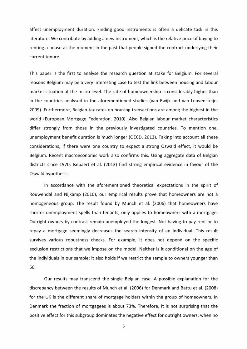
As to unemployment duration, we assume that the censoring times are stochastically

independent of the corresponding length of the unemployment spells and the explanatory

variables. The conditional likelihood of T, which is the unemployment duration as observed

in the dataset, of a particular individual can be described as11:

(1 ) ( )1x, , , exp exp exp1 2 1 1 1

c cT T Tf T z z v t t tT t t t

. (4)

This equation expresses the probability of leaving unemployment between T‐1 and T (first

factor of the RHS) if T is not censored, i.e. if c is 0. If T is censored, i.e. if c is 1, the likelihood

of T equals the survival probability.

The individual likelihood of y, the housing status at the start of the unemployment

spell of an individual, is given by:

Pr y , ,1 2

(1 )1 21 2Pr 1 , , Pr 2 , , 1 Pr 1 , , Pr 2 , ,1 1 1 12 2 2 2

u u

z zz zy u u y u u y u u y u u

x

x x x x

(5)

3.2.2.Integratedlikelihood

To obtain the unconditional likelihood contributions, we integrate the conditional

contributions over the unobserved heterogeneity distribution. In this respect, we adopt a

non‐parametric discrete distribution by analogy with Heckman and Singer (1984).12 We

estimate, in the spirit of van den Berg et al. (2002), our model for an optimal number K ‐

optimal according to reliable information criteria ‐ of heterogeneity types in the population

under investigation. Their proportions are specified as logistic transforms:

exp( )

exp( )1

qkpk Kq jj , with k = [1,K] and qk parameters to estimate (q1 normalized to 0). (6)

11 To avoid cumbersome notation, we simplified the notation for theta. 12 The methodology as advocated by these authors boils down to the assumption that a sample consists of a

finite number of subsamples with different levels of time‐invariant unobservable effects. Then, for all

subsamples the corresponding proportions are estimated as well as the impact of the unobserved differences

on the outcomes.

, with k = [1,K] and qk parameters to be estimated

(q1 normalized to 0). (6)

15

Besides the estimation of these proportions, this approach induces the estimation of one

mass point (location) for u1, u2 and v for each heterogeneity type: u1k, u2k resp. vk (u11, u21

resp. v1 are normalized to 0)13.14 Hence, the likelihood for an agent i is:

x, , , Pr y , ,1 12 21

Kl p f T z z v u uTi kk

x . (7)

We can then write the unconditional log‐likelihood as the sum of the unconditional

individual log‐likelihood contributions:

1

NL lii

. (8)

4.Results

4.1.Basicresults

Table 2 shows our main estimation results of the model. The Akaike Information Criterion

(AIC) indicates an optimal number of two heterogeneity types (K=2)15. Homeowners with

mortgage payments (who are the reference group) have ceteris paribus the shortest

unemployment spells. Outright owners, by contrast, stay unemployed the longest. Their

monthly probability to be re‐employed is 39% lower than the re‐employment probability of

owners with mortgage payments16. Our results are consistent with the intuition that having

to make a monthly payment increases the incentive of finding a job. Tenants have a 21%

lower probability to exit from unemployment each month compared to mortgagees.

13 We impose this normalisation since we allow for a constant term in the vector of observed characteristics x. 14 We take both the locations and the probabilities of the mass points to be unknown parameters without

constraining the correlation between u1, u2, and v. Allowing only perfect correlation or no correlation or a priori

limiting the number of heterogeneity types to an arbitrary number – the latter constraint is adopted in most of

the mentioned former contributions – may lead to biased estimates, as shown by Gaure et al. (2007). The

estimation procedure for gathering the probabilities and locations of the mass points is implemented according

to the latter authors. 15 Table A.2 in the Appendix reveals that the alternative information criteria (Hannan‐Quinn Information

Criterion and Bayesian Information Criterion) indicate an optimal number of only 1 type (K=1). Following the

argument in Gaure et al. (2007), we believe that the AIC is preferable when the sample is relatively small.

Nevertheless, we also report in Table A.3 in the Appendix (column 1) the estimation results of the main

coefficients in our model when we allow only one single heterogeneity type. The results are very similar to

those obtained from estimation with K=2. Note that Battu et al. (2008) also model two heterogeneity types.

Van Leuvensteijn and Koning (2004) specify three, Munch et al. (2006) no less than eight. 16 1 – exp(‐0.50) = 0.39.

16

Table 2: Unemployment duration and housing model – estimation results

Exit to employment Tenant Outright owner

Explanatory variables

Tenant ‐0.24 ** (0.11)

Outright owner ‐0.50 *** (0.18)

Constant ‐3.06 *** (0.45) 0.16 (0.99) 0.14 (1.23)

Woman ‐0.10 (0.10) 0.24 (0.19) ‐0.09 (0.22)

Foreign nationality ‐0.01 (0.13) 0.53 ** (0.26) ‐0.36 (0.41)

Age 16‐24 years 0.11 (0.18) 0.30 (0.33) 0.11 (0.47)

Age 25‐34 years 0.33 *** (0.11) ‐0.06 (0.22) 0.04 (0.34)

Age ≥ 50 years ‐0.84 *** (0.15) ‐0.14 (0.28) 1.62 *** (0.31)

Low educated ‐0.02 (0.12) 0.01 (0.22) ‐0.63 ** (0.28)

High educated 0.34 *** (0.11) ‐0.80 *** (0.22) ‐0.55 ** (0.26)

Cohabiting partner 0.33 ** (0.15) ‐0.71 *** (0.26) ‐0.35 (0.31)

Working partner 0.15 (0.14) ‐0.74 *** (0.25) ‐0.52 (0.29)

Having children younger than 18 ‐0.17 (0.11) ‐0.94 *** (0.20) ‐1.49 *** (0.27)

Densely populated area ‐0.06 (0.10) 0.64 *** (0.19) 0.45 * (0.24)

Brussels 2.55 ** (0.99) ‐3.01 (2.35) ‐0.10 (2.62)

Wallonia 1.50 *** (0.56) ‐1.59 (1.10) ‐1.01 (1.26)

Unemployment rate (province) ‐0.22 (2.06) 12.53 *** (4.56) ‐0.30 (6.20)

Unemployment rate (region) ‐1.08 *** (0.37) 0.42 (0.74) 0.46 (0.87)

% homeowners (province) 0.13 (0.37) 0.17 (0.48)

House price to rent ratio (province) 1.09 *** (0.15) ‐1.03 *** (0.27)

Duration dependence

t = [1] (ref.)

t = [2] 0.25 * (0.14)

t = [3] ‐0.11 (0.16)

t = [4,6] ‐0.41 *** (0.14)

t = [7,9] ‐0.88 *** (0.18)

t = [10,12] ‐0.40 ** (0.17)

t = [13,15] ‐0.94 *** (0.28)

t > 15 ‐1.68 *** (0.26)

Unobserved heterogeneity: estimates

v2/u1,2/u2,2 0.80 (1.31) ‐20.00 8.81 (8.19)

q2 ‐3.99 *** (0.76)

Unobserved heterogeneity: resulting probabilities and correlation

p1 0.98

p2

Corr(v,u1)

Corr(v,u2)

Corr(u1,u2)

0.02

‐1.00

1.00

‐1.00

Log‐likelihood ‐2645.44

Akaike Information Criterion 5420.89

Parameters 65

N 1013

***(**)((*)) indicates significance at the 1%(5%)((10%)) significance level. Standard errors in parentheses. Some heterogeneity parameters are estimated as a very large negative or positive number causing a 0 or 1 probability with respect to related housing tenure status for a subset of individuals. This is numerically problematic. When we face this problem, in the spirit of Gaure et al. (2007), we mark the offending parameter as ‘infinity’, stick it to ‐20 resp. 20, and keep it out of further estimation.

17

The outlined results underline the importance of distinguishing outright owners and

mortgagees for an adequate analysis of the relationship between housing and labour market

outcomes. In particular, they confirm the hypotheses that we derived from Rouwendal and

Nijkamp (2010) in the introduction to this paper. Furthermore, they may help to understand

the mixed findings in former contributions that did not distinguish the two types of owners.

The very high fraction of mortgagees in Denmark (73%) may explain why Munch et al. (2006)

find faster exit rates for owners than for tenants. Along the same line of thought, the more

balanced composition of the group of owners in the UK, where only 56% are mortgagees,

may explain why Battu et al. (2008) find no significant difference in the exit rates of owners

and private tenants17. In Table 1 we reported data on the composition of the group of

owners in Belgium. With 64.6% of them holding a mortgage, Belgium takes a position

somewhat in the middle between the UK and Denmark. The empirical results that we

present in Table A.4 in the Appendix should then come as no surprise. The table contains the

outcome of a more restricted version of our model in which we do not distinguish between

both categories of homeowners. Merging outright owners and mortgagees, we find no

significantly different exit rate from unemployment compared to tenants anymore. This

result is in line with Battu et al. (2008).

Although our methodology does not allow interpreting the coefficients of the other

explanatory variables structurally, their sign and level of statistical significance reveal some

information about the control variables. The observed effects on unemployment duration on

the left side of Table 2, are generally consistent with our expectations. Ceteris paribus,

unemployment spells tend to last longer for individuals who are older than 50, not highly

educated and not cohabiting. Although the latter is also found by Munch et al. (2006) and

Battu et al. (2008), it might seem rather odd. A possible explanation could be the

appearance of positive network effects that are associated with having a partner. Also,

unemployment replacement rates are slightly lower when cohabiting18. Last, we see that

regional dummies and the regional unemployment rate help to determine unemployment

duration as well.

17 The percentages that we mention have been derived from the EU‐SILC database by Dol and Neuteboom

(2009). 18 Data are available from Van Vliet and Caminada (2012).

18

The other columns of Table 2 show the results of the simultaneously estimated mixed

multinomial logit model for housing tenure. Also for this component of our model, the

coefficients of the explanatory variables show the expected sign. We are particularly

interested in the performance of the selected instruments. The percentage of homeowners

in the province has only low explanatory power. A possible explanation might be the large

scale of the province, summing away most variation. In earlier studies, the municipality was

selected as the aggregate level allowing for more variation. Much higher predictive power is

attained by the provincial relative price of buying a house versus renting in the year of

contract/purchase. In line with our expectations, a high ratio causes a higher probability of

renting and a lower probability of being an outright owner.

4.2.Additionalresultsandrobustnesschecks

We conducted several sensitivity analyses to test the robustness of our main finding, i.e. the

longer unemployment duration for outright owners compared to tenants and mortgagees.

Table A.3 in the Appendix shows the estimated coefficients and corresponding standard

errors for our main variables of interest. We summarize the results here:

‐ We re‐estimated our basic model first omitting one of the two instruments while

maintaining the other. Then we re‐estimated the model without including any

instruments. The main results of the three additional estimations are shown in

columns (2), (3) and (4) of Table A.3. The results without the provincial

homeownership rate as instrument are close to the benchmark model. When not

including the house price to rent ratio in the year of purchase or contract, the

standard errors increase and so does the estimated coefficient for outright owners.

The difference between homeowners with a mortgage and tenants is no longer

significant. These results are close to those in column (4), the model without

instruments. These findings underscore the importance of introducing the innovative

relative price of owning versus renting as an instrument.

‐ We re‐estimated our model dropping all individuals older than 50 from our sample. As

was clear from our description of the data in Section 2, there is a strong correlation

between being older than 50 and being an outright owner. Although we control for

age in our estimations, it could be advisable to check whether our results are not in

19

some way driven by this age group. As is well‐known, and confirmed in Table 2,

people older than 50 have typically longer unemployment spells. When we drop

individuals older than 50, all our basic findings survive. We report the main results of

this re‐estimation in column (5) of Table A.3.

‐ Finally, we introduced alternative age variables in column (6). More precisely, instead

of four crude age categories, we directly included individuals’ age and its square as

continuous explanatory variables. All our basic findings again survive.

5.Conclusions

Seminal work by A.J. Oswald (1996, 1997) suggests that homeownership impairs an

individual’s labour market outcome. A key element is that high costs of buying and selling

homes make homeowners less geographically mobile, which reduces the number of suitable

vacancies within their reach in the case of job loss. Homeowners should therefore be

expected to incur longer unemployment spells than tenants. Existing microeconometric

research for the UK and Denmark, however, comes to different conclusions. Battu et al.

(2008) find no significant difference in the speed of transition from unemployment into

employment among homeowners versus private tenants in the UK. Munch et al. (2006) even

observe a faster exit from unemployment into employment among owners than among

tenants in a large panel of Danish individuals.

This paper examines the impact of housing tenure choice on unemployment duration in

Belgium using EU‐SILC micro data for 2003‐2008. Our research question and methodology

are basically the same as those of the aforementioned studies. We contribute to the

literature in distinguishing homeowners with mortgage payments and outright homeowners.

We simultaneously estimate unemployment duration by a mixed proportional hazard model,

and the probability of being an outright homeowner, a homeowner with mortgage payments

or a tenant by a mixed multinomial logit model. To be able to correctly identify the causal

influence of different types of housing tenure on unemployment duration, we use

instrumental variables. Finding good instruments is always a delicate task. We propose a

new (and strong) instrument, which is the relative price of buying versus renting a house at

the moment in the past that people signed the contract underlying their current tenure.

20

Our results show that homeowners with a mortgage exit unemployment first. Outright

owners stay unemployed the longest. Tenants take an intermediate position. From the point

of view of the Oswald hypothesis these findings cannot be rationalized as the search and

transaction costs associated with moving are similar for outright owners and mortgagees.

Instead, our results support the theoretical framework developed by Rouwendal and

Nijkamp (2010) and the role of housing costs. If the latter are high, liquidity constraints and

the induced reduction of consumption generate strong incentives for the unemployed to

find a job soon. Search intensity will be high, the unemployment spell short. If housing costs

are low, by contrast, search behaviour will be less intense and the unemployment spell

longer. The fact that ceteris paribus the monthly burden of housing costs is much higher for

mortgagees than for outright owners, with tenants again in the middle (although

undoubtedly closer to mortgagees) can rationalize our empirical findings.

Our results also provide a possible explanation for the discrepancy between the former

contributions to this literature. When the distinction between both groups of homeowners is

not taken into account, the perceived effect of homeownership will basically be the result of

the composition of the group of owners. A much higher share of mortgage holders within

the group of homeowners in Denmark compared to the UK may explain the different

findings of Munch et al. (2006) versus Battu et al. (2008).

21

AppendixA:Additionaltables

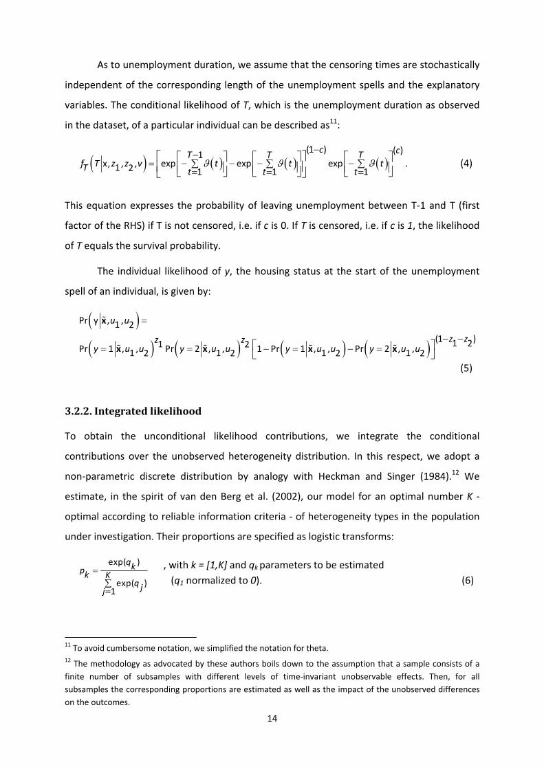
Table A.1: Definitions of variables

Variable name Definition

Tenant Dummy equals 1 if the household rents the house.

Outright owner Dummy equals 1 if the household owns the house and no mortgage payments have to be made.

Mortgagee Dummy equals 1 if the household owns the house and pays off a mortgage.

Woman Dummy equals 1 for females, 0 for males.

Foreign nationality Dummy equals 1 if the individual has a foreign nationality, 0 if not.

Age 16‐24 years Dummy equals 1 if the individual is 16‐24 years old.



Age ≥ 50 years Dummy equals 1 if the individual is ≥ 50 years old.

Low educated Dummy equals 1 if the individual did not finish secondary education.

Middle educated Dummy equals 1 in case of a secondary or post‐secondary non tertiary degree.

High educated Dummy equals 1 in case of a tertiary degree.

Cohabiting partner Dummy equals 1 if the individual lives together with a partner, 0 otherwise.

Working partner Dummy equals 1 if the individual lives together with a working partner, 0 if not.

Having children younger than 18 Dummy equals 1 if the person has children younger than 18, 0 otherwise.

Densely populated area Dummy equals 1 if the individual lives in a municipality with a density superior to 100 inhabitants per square kilometer, and either with a total population for the set of at least 50,000 inhabitants or adjacent to a densely‐populated area.

Brussels Dummy equals 1 when living in the region Brussels.

Flanders Dummy equals 1 when living in the region Flanders.

Wallonia Dummy equals 1 when living in the region Wallonia.

Unemployment rate (province) Unemployment rate in the province (continuous number between 0 and 1).

Unemployment rate (region) Unemployment rate in the region (continuous number between 0 and 1).

% homeowners (province) Percentage of homeowners in the province of residence.

House price to rent ratio in year of contract (province)

Ratio of the provincial house price index (with Belgium1990=100) to the rent index (with Belgium1990=100), calculated in the year of purchase or contract.

Note: As explained in the text, values are fixed at the start of the unemployment spell for all variables except for the regional unemployment rate.

22

Table A.3: Unemployment duration and housing model – Sensitivity Analysis

Exit to employment

(0) (1) (2) (3) (4) (5) (6)

Benchmark results (Table 2)

Estimating the

benchmark model with

K=1

Omitting provincial rate of

homeowner‐ship as

instrument

Omitting historical house price to rent ratio as

instrument

Estimating without

instruments

Omitting individuals older than 50 from the sample

Including age and age² as continuous explanatory variables

Tenant ‐0.24 ** (0.11) ‐0.24 ** (0.11) ‐0.24 ** (0.11) ‐0.22 (0.32) ‐0.23 (0.32) ‐0.27 ** (0.11) ‐0.24 ** (0.11)

Outright owner ‐0.50 *** (0.18) ‐0.40 *** (0.13) ‐0.50 *** (0.18) ‐0.81 ** (0.41) ‐0.82 ** (0.41) ‐0.54 ** (0.23) ‐0.48 *** (0.18)

Optimal K 2 ‐ 2 3 3 2 2

Log‐likelihood ‐2645.44 ‐2654.28 ‐2645.56 ‐2701.89 ‐2703.20 ‐2033.56 ‐2643.29

AIC 5420.89 5430.57 5417.11 5537.78 5536.36 4191.11 5410.57

Parameters 65 61 63 67 65 62 62

N 1013 1013 1013 1013 1013 739 1013


Table A.2: Model selection (benchmark model)

# param. Log‐likelihood AIC HQIC BIC

1 type 61 ‐2654.283 5430.566 6152.887* 5730.726*

2 types 65 ‐2645.444 5420.888* 6190.575 5740.732

3 types 69 ‐2642.842 5423.684 6240.7371 5763.211

4 types 73 ‐2639.318 5424.635 6289.053 5783.844

5 types 77 ‐2638.714 5431.428 6343.211 5810.320

Note: *: Preferred specification by this criterion. AIC: Akaike Information Criterion. HQIC: Hannan‐Quinn Information Criterion. BIC: Bayesian Information Criterion.

23

Table A.4: Unemployment duration and housing model (restricted) – estimation results

Exit to employment Tenant

Explanatory variables

Tenant ‐0.05 (0.12)

Constant ‐3.30 *** (0.44) ‐0.68 (0.97)

Woman ‐0.09 (0.09) 0.26 (0.18)

Foreign nationality ‐0.01 (0.13) 0.64 *** (0.25)

Age 16‐24 years 0.10 (0.17) 0.34 (0.30)

Age 25‐34 years 0.33 *** (0.10) ‐0.07 (0.22)

Age ≥ 50 years ‐0.99 *** (0.15) ‐0.88 *** (0.26)

Low educated 0.01 (0.12) 0.22 (0.21)

High educated 0.36 *** (0.10) ‐0.63 *** (0.21)

Cohabiting partner 0.35 ** (0.14) ‐0.63 *** (0.24)

Working partner 0.20 (0.13) ‐0.64 *** (0.24)

Having children younger than 18 ‐0.11 (0.10) ‐0.57 *** (0.20)

Densely populated area ‐0.10 (0.09) 0.54 *** (0.18)

Brussels 2.64 *** (0.92) ‐3.02 (2.16)

Wallonia 1.56 *** (0.51) ‐1.33 (1.02)

Unemployment rate (province) ‐0.55 (2.03) 14.00 *** (4.89)

Unemployment rate (region) ‐1.10 *** (0.34) 0.26 (0.70)

% homeowners (province) 0.12 (0.35)

House price to rent ratio (province) 1.44 *** (0.18)

Duration dependence

t = [1] (ref.)

t = [2] 0.26 * (0.13)

t = [3] ‐0.10 (0.16)

t = [4,6] ‐0.41 *** (0.14)

t = [7,9] ‐0.87 *** (0.18)

t = [10,12] ‐0.39 ** (0.17)

t = [13,15] ‐0.95 *** (0.27)

t > 15 ‐1.69 *** (0.26)

Unobserved heterogeneity: estimates

v2/u2 0.66 (0.54) ‐20.00

q2 ‐2.64 *** (0.61)

Unobserved heterogeneity: probabilities and correlation

p1 0.933

p2

Corr(v,u)

0.067

‐1.00

Log‐likelihood ‐2348.70

Akaike Information Criterion 4785.39

Parameters 44

N 1013


24

References

Battu H., Ma A. and E. Phimister, 2008, “Housing tenure, job mobility and unemployment in the UK”, Economic Journal, 118, pp.311‐328.

Böheim R. and M. Taylor, 2002, “Tied down or room to move? Investigating the relationships between housing tenure, employment status and residential mobility in Britain”, Scottish Journal of Political Economy, 49, n°4, pp.369‐392.

Caldera Sánchez A. and D. Andrews, 2011, “Residential Mobility and Public Policy in OECD Countries”, OECD Journal: Economic Studies, Vol. 2011/1, pp.185‐206.

Coulson E.N. and L.M. Fisher, 2002, “Tenure Choice and Labour Market Outcomes”, Housing Studies, 17, pp.35‐50.

Coulson E.N. and L.M. Fisher, 2009, “Housing tenure and labor market impacts: The search goes on”, Journal of Urban Economics, 65, pp.252‐264.

Dol K. and P. Neuteboom, 2009, “Macro Change and Micro Behaviour: the effects of aging on tenure choice, and households’ strategies towards the use of housing wealth”, DEMHOW Research Paper, Delft.

European Mortgage Federation, 2010, “Study on the Cost of Housing in Europe”, Brussels.

Flatau P., Forbes M., Hendershott P.H. and G. Wood, 2003 “The roles of leverage and public housing”, NBER Working paper, n°10021.

Gaure S., Roed K. and T. Zhang, 2007, “Time and causality: A Monte Carlo assessment of the timing‐of‐events approach”, Journal of Econometrics, 141, pp.1159‐1195.

Goss, E.P. and J.M. Phillips, 1997, “The Impact of Home Ownership on the Duration of Unemployment”, Review of Regional Studies, 27, pp.9‐27.

Heckman J.J. and B. Singer, 1984, “A Method for Minimizing the Impact of Distributional Assumptions in Econometric Models for Duration Data”, Econometrica, 52, pp.271‐320.

Heylen K., Le Roy M., Vandenbroucke S., Vandekerckhove B. and S. Winters, 2007, “Wonen in Vlaanderen. De resultaten van de woonsurvey 2005 en de uitwendige woningschouwing 2005”, Kenniscentrum voor een Duurzaam Woonbeleid/Vlaamse overheid, Brussel, 483p.

Hughes G. and B. McCormick, 1981, “Do council housing policies reduce migration between regions?”, The Economic Journal, 91, pp.919‐937.

25

Hughes G. and B. McCormick, 1987, “Housing markets, unemployment and labour market flexibility in the UK”, European Economic Review, 31, pp.615‐645.

Isebaert D., 2013, “Housing tenure and geographical mobility in Belgium”, Faculty of Economics and Business Administration Working Paper, Ghent University, n° 2013/855.

Isebaert D., Heylen F. and C. Smolders, 2013, “Houses and/or jobs: ownership and the labour market in Belgian districts”, Regional Studies, forthcoming.

Kiefer N., 1988, “Economic Duration Data and Hazard Functions”, Journal of Economic Literature, 26, pp.646‐679.

Munch J.R., Rosholm M. and M. Svarer, 2006, “Are homeowners really more unemployed?”, The Economic Journal, 116, pp.991‐1013.

Munch J.R., Rosholm M. and M. Svarer, 2008, “Home ownership, job duration, and wages”, Journal of Urban Economics, 63, pp.130‐145.

OECD, 2012, Employment Outlook, OECD, Paris.

OECD, 2013, “Benefits and wages”, http://www.oecd.org/els/benefitsandwagesstatistics.htm

Oswald A.J., 1996, “A conjecture on the explanation for high unemployment in the industrialized nations: part 1”, Warwick Economic Research Papers, n° 475, University of Warwick.

Oswald A.J., 1997, “Thoughts on Nairu”, Journal of Economic Perspectives, 11, n°1, pp.227‐228.

Pittini A. and E. Laino, 2011, “Housing Europe Review 2012, The nuts and bolts of European social housing systems”, CECODHAS Housing Europe’s Observatory, Brussels.

Rouwendal J. and P. Nijkamp, 2010, “Homeownership and labour‐market behavior: interpreting the evidence”, Environment and Planning A, 42, pp.419‐433.

van den Berg J., Holm A. and J.C. van Ours, 2002, “Do stepping‐stone jobs exist? Early career paths in the medical profession”, Journal of Population Economics, 15, pp.647‐665.

van Ewijk C. and M. van Leuvensteijn, 2009, “Introduction and Policy Implications”, In: van Ewijk C. and M. van Leuvensteijn (eds.), Homeownership & the Labour Market in Europe, Oxford University Press, New York, pp.1‐11.

26

van Leuvensteijn M. and P. Koning, 2004, “The effect of home‐ownership on labor mobility in the Netherlands”, Journal of Urban Economics, 55, pp.580‐596.

Van Vliet O. and K. Caminada, 2012, “Unemployment replacement rates dataset among 34 welfare states 1971‐2009: An update, extension and modification of the Scruggs. Welfare State Entitlements Data Set”, NEUJOBS Special Report, n°2, Leiden University.

Vastmans F. and E. Buyst, 2011, “Woningprijzen in Vlaanderen en de rol van de intrestvoet”, In: Winters S. (ed.), Is wonen in Vlaanderen betaalbaar?, Garant, Antwerpen/Apeldoorn, pp.15‐48.

Does Homeownership Lead to Longer Unemployment Spells…ftp.iza.org/dp7774.pdf · Does...

Documents

Transcript of Does Homeownership Lead to Longer Unemployment Spells…ftp.iza.org/dp7774.pdf · Does...