FEDERAL RESERVE BANK OF SAN FRANCISCO

WORKING PAPER SERIES

Does Disappointing European Productivity Growth Reflect a Slowing Trend? Weighing the Evidence and Assessing the Future

John Fernald

INSEAD Federal Reserve Bank of San Francisco

Robert Inklaar

University of Groningen

May 2020

Working Paper 2020-22

https://www.frbsf.org/economic-research/publications/working-papers/2020/22/

Suggested citation:

Fernald, John, Robert Inklaar. 2020. “Does Disappointing European Productivity Growth Reflect a Slowing Trend? Weighing the Evidence and Assessing the Future,” Federal Reserve Bank of San Francisco Working Paper 2020-22. https://doi.org/10.24148/wp2020-22 The views in this paper are solely the responsibility of the authors and should not be interpreted as reflecting the views of the Federal Reserve Bank of San Francisco or the Board of Governors of the Federal Reserve System.

Does disappointing European productivity growth reflect a slowing trend? Weighing the evidence and assessing the future*

John Fernald

INSEAD and the Federal Reserve Bank of San Francisco

Robert Inklaar University of Groningen

May 2020

Abstract

In the years since the Great Recession, many observers have highlighted the slow pace of labor and total factor productivity (TFP) growth in advanced economies. This paper focuses on the European experience, where we highlight that trend TFP growth was already low in the runup to the Global Financial Crisis (GFC). This suggests that it is important to consider factors other than just the deep crisis itself or policy changes since the crisis. After the mid-1990s, European economies stopped converging, or even began diverging, from the U.S. level of TFP. That said, in contrast to the United States, there is some macroeconomic evidence for some northern European countries that the GFC had a further adverse impact on TFP growth. Still, the challenges for economic policy look surprisingly similar to the ones discussed prior to the Great Recession, even if the policy implications seem less clear.

Keywords: Productivity Growth; Great Recession; Convergence JEL Codes: D24, E23, E44, F45, O47

* john.fernald@insead.edu and r.c.inklaar@rug.nl. We thank Bart van Ark, Andrew Sharpe, Ilya Voskoboynikov, and participants at the IARIW 2018 conference and the 2020 AEA session on “Sources of the Transatlantic Productivity Slowdown” for helpful comments. We thank Mitchell Ochse for excellent research assistance. The views in this paper are those of the authors and do not necessarily reflect the views of the Federal Reserve Bank of San Francisco or anyone else associated with the Federal Reserve System.

1. Introduction

Across advanced economies, the recovery from the Great Recession was disappointingly slow. Initially, observers pointed primarily to temporary disruptions and dislocations from the crisis itself. But as the recovery continued, GDP growth remained subdued. Well before the massive 2020 health and economic shock from COVID-19, there was an increasing recognition that trend output growth rates were slow. For Europe as well as the United States, the “surprise,” relative to expectations from the pre-2007 period, has been in labor productivity. After all, the demographics of an aging population were largely foreseen.1

We survey the European productivity experience from a macroeconomic perspective. We argue that the slow trend is not simply the “long shadow” (Fatás, 2000) cast by the Global Financial Crisis (GFC)—as disruptive as that event was. Indeed, both labor and total factor productivity (TFP) were slowing prior to the GFC. Statistical break tests on TFP growth do provide some tentative evidence of a post-2007 break for at least some northern European economies. But even if the GFC did lead to some further decline in trend TFP growth, that growth rate was already relatively modest.

Figure 1 illustrates the slowing TFP trend. The data are a weighted average of TFP growth for the 15 pre-2004 European Union countries from the Penn World Tables (PWT, Feenstra et al., 2015). TFP growth has been slowing since the 1960s. Of course, much of that slowdown was benign, reflecting the end of the convergence “boost” that Europe received after World War II. But, as we discuss, the further slowdown since the 1990s reflects a different pattern. Some countries have been falling rapidly away from the frontier (notably Spain and Italy). In Northern Europe, countries stopped converging short of U.S. levels, or have even (depending on the dataset) drifted gradually down relative to the United States.2

Figure 1 shows two estimated trend lines from a biweight filter. This filter is close to a 12-year centered moving average that becomes increasingly one-sided at the end points. The red-dashed line uses data through 2017. The full-sample TFP trend falls to near zero growth by 2005 and remains there. Of course, the pre-2007 values of the full-sample filter are pulled down by the sharp negative growth that subsequently occurred in 2008 and 2009. For this reason, the maroon-dashed line is estimated using data through 2007 only. That quasi-real-time trend line lies above the

1 For major European economies, which is our focus, labor-force growth from 2010-2019 has actually exceeded the (slow) projections by the European Commission (Carone et al., 2006), reflecting increases in labor-force participation (Gros, 2019). But labor productivity has fallen short of 2006 projections. 2 Cette et al. (2016) found, using data from Bergeaud et al. (2016), that total economy TFP levels in major European countries were similar to U.S. levels by the mid-1990s, but subsequently lost ground relative to U.S. levels. PWT, Conference Board (2019), and OECD data also show that TFP growth in most European countries fell short of the U.S. pace from 1995-2007. In contrast, in market-sector EU KLEMS (2017) data that we use for some of our analysis below, TFP growth in Northern Europe was very close to the U.S. pace from 1995-2007. In any case, we find that the level of market-sector TFP for major European economies was uniformly below the U.S. level after the early 1990s. Even in EU KLEMS, northern European countries lost ground relative to the U.S. over the full 1995-2015 period.

2

estimated full-sample trend after the late 1990s. But it nevertheless stood at only 0.4 percent per year on the eve of the 2007-9 Great Recession, down from 0.9 percent in the early 1990s.

Indeed, before the recession, a large literature addressed the puzzle that Europe had seen a mid-1990s productivity slowdown even as the U.S. had seen a pickup. Timmer, et al., (2010) reviewed the pre-GFC debate. They concluded that European economies had not fully adapted to a knowledge-based economy, in terms of flexibility, skills, management, and such. Cette et al. (2016), similarly emphasize the pre-GFC origins of slowing TFP growth in Europe.

For most of the paper, we focus on TFP growth, which adjusts for observable capital growth as well as the educational qualifications of the workforce. The reason is that the source of weak labor productivity growth has been the anemic pace of TFP growth. We find that weak capital formation—investment in plant, equipment, software, and the like—has played at most a small direct role. Capital-output ratios, in particular, do not look low relative to pre-recession trends.

In the United States, the leading hypothesis for the disappointing output recovery after the Great Recession is that the deep recession was superimposed on a sharply slowing output growth trend. That slow trend, in turn, was largely independent of the Great Recession itself (Fernald et al., 2017). The mid-1990s productivity boom ended several years prior to the Great Recession (Fernald, 2014; Fernald et al., 2017). For example, quarterly TFP growth from the end of 2004 through 2007 was slower than it was from the end of 2007 through 2019. In addition, the U.S. slowdown was observed before the recession, and professional forecasters were already at least partially accounting for it (Fernald et al., 2017). Information and communications technology (ICT) had provided an exceptional boost to trend TFP growth in the mid-1990s and early 2000s. The waning trend plausibly reflected a pause in (if not the end of) those exceptional gains.

Consistent with this view, Bloom et al. (2020) argue that “ideas are getting harder to find” (Bloom et al., 2020). Closely related, Aghion et al. (2019) and de Ridder (2020) provide endogenous-growth models in which the initial gains from ICT eventually lead to reduced innovation throughout the economy as well as reduced dynamism. For the United States, the best guess at this point is thus that trend growth remains low (Fernald and Li, 2019). 3

We view Europe’s experience as broadly consistent with the same narrative. The unusually deep and long recession was superimposed on a slowing productivity trend. Unlike the U.S. case, though, there is some evidence that the GFC might have led to a further decline in TFP growth in

3 There are complementary stories that emphasize regulation. For example, Fernández-Villaverde and Ohanian (2018) argue that regulation and a lack of competition have led to weak growth in Europe as well as the United States. That said, Fernald et al. (2017) find no quantitative evidence that regulatory changes have a first-order impact on U.S. TFP growth. Philippon (2019) argues that Europe is now more competitive than the United States.

3

some countries. But even in Europe, pre-2007 trend growth was slower than in the late 1990s, let alone the late 1980s.4

Conceptually, Europe’s TFP trend reflects not only the U.S. trend, but also “distance to the frontier.” Many countries in Europe have either remained short of the frontier—as we find here—or else fell further behind the frontier. From a conditional convergence perspective, it remains unclear where to pin a new steady state for many European economies relative to the United States—and indeed, one challenge is to characterize the disparate pattern across European economies. While Northern European countries have modestly lost ground relative to the United States, Southern European countries have lost considerable ground since the 1990s. There is little evidence that countries in Europe are closing the gap with the United States.5

The primary alternative to our ‘slowing underlying trend’ view is the hypothesis that the productivity slowdown was, in fact, primarily a result of the GFC. There is no question that the crisis was a traumatic and disruptive event across advanced economies. Fatás and Summers (2018) find a permanent effect of the crisis on potential output in many or most countries. There are many channels through which such hysteresis could work, with TFP being one of them.6 A superficial look at the data does suggest reasons for focusing on TFP effects: Major European economies have had very weak (if not negative) average TFP growth since 2007.7 Drawing direct conclusions based on these weak growth rates is hard, however, because recessions often lead to a decline in measured TFP growth. Factor utilization (labor effort and capital’s workweek) tends to fall in recessions but is not directly observed in the standard input measures.

But a deep recession could have persistent, adverse effects on TFP growth (e.g., Adler et al, 2017). Possible channels include reduced incentives to innovate (e.g., Bianchi et al., 2018; Anzoategui et al., 2019; Garga and Singh, 2020); increased misallocation of resources in some economies (e.g.,

4 Fernald (2018) provides an earlier view on this topic, discussing evidence for the United States and other advanced economies. The conclusion in that paper also emphasized the pre-GFC productivity growth slowdown. In contrast to the current paper, it played down the role of the GFC itself. 5 See also Gordon and Sayed (2019). They argue that Europe has been catching up to the United States in stages. They note that the “early to late” slowdown in labor productivity growth was similar in western Europe and the United States—but the “early” U.S. period was pre-1973, whereas the early European period was 1972-95. 6 Oulton and Sebastiá-Barriel (2017) survey the literature and provide estimates of several of the channels. Conceptually, hysteresis in output growth reflects either hysteresis in labor input, or hysteresis in labor productivity. On the labor side, workers who spend an extended period unemployed may well lose labor-market skills; because they are harder to employ, the natural rate of unemployment rises. Workers may also lose attachment to the labor market and move out of the labor force. In term of labor productivity, we discuss capital deepening and TFP below. 7 In the Conference Board’s (2019) Total Economy Database, aggregate TFP growth in virtually all European economies was zero or negative in the 2007-2018 period (exceptions were Germany, Iceland, Ireland, and Malta). In the EU KLEMS 2017 market economy from 2007-2015, TFP growth in all countries other than Belgium was negative (see Figure 4). In the PWT from 2007-2017, for the same set of countries, only Germany had positive TFP growth. In OECD data for 2007–2018, most European countries show growth rates close to zero (ranging from –0.1% per year to +0.1% per year), with the exceptions of Denmark (+0.5%), Germany (+0.5%), Ireland (+1%), Italy (–0.3%), Luxembourg (–0.8%) and Greece (–1.9%).

4

Gopinath et al. 2017); or increased credit frictions that further reduce investment in intangibles such as R&D, organization capital, and training (e.g., Duval et al., 2017).

But even if these factors are important, the evidence from Figure 1 and later sections of this paper suggest that any effects of the GFC were on top of an already-slowing TFP trend. This is particularly true relative to the United States, where the pre-recession timing of the TFP slowdown is well established. At a minimum, these facts suggest limits to some popular stories in which the Great Recession caused the slow pace of productivity growth.

This paper is structured as follows. Section 2 documents some key facts that inform the debate. We focus especially on TFP growth because, as we discuss, we do not see weak capital formation as an important independent channel for explaining weak growth in labor productivity. Section 3 examines break tests on TFP growth. We find some evidence for some countries pointing to a structural break after 2007, but this partly depends on the dataset and level of aggregation. Section 4 looks at cyclical aspects of TFP dynamics. It is challenging, in the European context, to control for cyclical effects directly because of the heterogeneity in institutions and the lack of suitable proxies for cyclical mismeasurement. Cyclical mismeasurement issues might still affect the EU KLEMS numbers we use through 2015, but they had plausibly run their course by the end of the PWT sample in 2017. Section 5 draws upon the literature and discusses evidence on various additional issues that could affect how we interpret the TFP growth slowdown, including vintage capital models, demographics, market power, and intangible capital. Section 6 discusses how to interpret the facts and draws some lessons for the future.

2. Keyfactsandconceptualframework

This section starts by motivating our focus on TFP growth. Weak TFP growth is the key to understanding weak labor productivity growth across Europe. Specifically, we find that a shortfall of capital formation was not an important independent contributor to weak labor productivity growth. We then highlight some of the differences in TFP levels and growth rates across countries and discuss how the trends fit into a framework of conditional convergence.

The takeaways are that TFP is the right place to look for understanding weak labor productivity growth in Europe; that the pace was slowing and heterogeneity across countries was rising even before the Great Recession; and that stories that focus on particular sectors in particular countries (e.g., construction in Spain) won’t explain the broad-based slow pace of TFP growth.

A. Accounting for European labor productivity: TFP and capital deepening

Table 1 shows two complementary growth-accounting decompositions since 1985 for the PWT and EU KLEMS datasets. In both cases, the accounting covers a European aggregate. PWT covers the entire economy, whereas EU KLEMS (which merges the 2012 and 2017 vintages) shows the

5

market sector.8 EU KLEMS covers Austria, Finland, France, Germany, Italy, the Netherlands, Spain, the United Kingdom for a sufficiently long period. PWT has more data availability, covering all 15 countries that were members of the European Union prior to 2004—which adds Belgium, Denmark, Greece, Ireland, Portugal, and Sweden. Within each dataset, output, capital, hours, TFP, and labor composition are appropriate PPP-adjusted Törnquist aggregates.

Line 1 of each panel in the table shows that, broadly speaking, labor productivity growth has fallen steadily over time. For example, in PWT, labor productivity grew 2.5 percent per year in the 1985–1995 period, 1.5 percent in the 1995–2007 period, and only 0.7 percent in the 2007–17 period.

Looking at shorter subperiods in columns 4 to 7, the exception to the steady decline is that labor productivity growth was particularly weak in the 2007–11 period and rebounded somewhat in the 2011–17 period. That period runs from one euro-area business-cycle peak to another. But the rebound from the deep 2008–9 recession was incomplete by 2011. So cyclical influences on productivity were still pronounced over this subperiod, a topic we return to in Section 4.

The table then shows two complementary growth-accounting decompositions of labor productivity. Both decompositions start with the basic growth-accounting identity that implicitly defines TFP growth, 𝛥 ln 𝑇𝐹𝑃!:

𝛥 ln 𝑌! = 𝛼!𝛥 ln𝐾! + (1 − 𝛼!)(𝛥 ln𝐻! + 𝛥 ln 𝐿𝐶!) + 𝛥 ln 𝑇𝐹𝑃! . (1)

In this equation, 𝛥 ln 𝑌! is output growth, 𝛥 ln𝐾! is capital growth, 𝛥 ln𝐻! is hours growth, and 𝛥 ln 𝐿𝐶! is labor composition growth. 𝛼! is the nominal share of payments to capital in revenue (which, in practice, we take to be the average in years 𝑡 − 1 and 𝑡), and (1 − 𝛼!) is labor’s share. We assume the factor shares sum to one.9

Rearranging equation (1) yields our first decomposition, shown in lines 2 to 4 of Table 1:

𝛥 ln 𝑌! − 𝛥 ln𝐻! = 𝛼!(𝛥 ln𝐾! − 𝛥 ln𝐻!) + (1 − 𝛼!)𝛥 ln 𝐿𝐶! + 𝛥 ln𝑇𝐹𝑃! . (2)

8 The main takeaways are robust across these and other datasets shown in the data appendix. The additional datasets are the Conference Board’s Total Economy Database (TED) and the OECD. The data appendix also shows data from the 2019 vintage of EU KLEMS (Stehrer, 2019). The 2019 vintage starts in 1995 but appears inconsistent with the 2012 vintage, so it is not appropriate to merge them. More concerningly, the capital data in the ‘statistical database’ of the 2019 vintage (which, like other sources, includes only national accounting intangibles), is quite different from other sources—growing more slowly throughout the period since 1995. Pending further analysis of the sources of the differences, we have chosen to include the 2019 vintage in the data appendix but not the main text. For the 2012 and 2017 versions of the EU KLEMS database, see www.euklems.net. For the 2019 version, see www.euklems.eu. 9 Under standard conditions of constant returns to scale, perfect competition, and perfect factor mobility (Solow, 1957), TFP growth defined by this equation represents the outward shift in society’s production possibilities frontier from technological change. A large literature has explored the interpretation of TFP growth when these conditions fail (e.g., Basu and Fernald, 2002; Oulton, 2016). For our purposes, we simply take equation (1) as implicitly defining aggregate TFP growth as the part of aggregate output growth that is not explained by revenue-share-weighted growth in capital and labor inputs.

6

The first term captures the contribution of changes in the ratio of capital to hours. Intuitively, workers have more “tools” to work with, they will be more productive per hour worked. The second term is the direct contribution of changes in labor composition. This term captures changes in the educational qualifications of the labor force; for example, workers with more education or experience are typically more productive. The third term is standard TFP growth.

With this first decomposition, the vast majority of the slowdown in labor productivity after 2007 occurs through slower TFP growth (line 4). Looking at the PWT data, TFP growth falls from 0.95 percent per year from 1985–95 (column 1) to 0.47 percent from 1995–2007, to –0.12 percent per year from 2007–2017 (column 3). The sharp slowdown in TFP growth is also apparent in the EU KLEMS market sector—where TFP growth slows almost a percentage point (from +0.65 percent to -0.30 percent). In EU KLEMS, capital deepening slows somewhat more than in PWT after 2007 (where the contribution in line 2 falls about 0.2 percentage points). But in both cases, after 2007, slower growth in capital deepening (line 2) is only a modest to moderate contributor to the labor productivity slowdown. A slowdown in labor composition growth (line 3) contributes even less to the slowdown. Indeed, in EU KLEMS, labor composition grows more quickly after 2007.

This decomposition arguably overstates the contribution of capital deepening to the labor-productivity slowdown because of the endogeneity of capital. For example, in the Solow (1956) growth model, all growth in output per hour comes from TFP growth. But equation (2)—which closely follows Solow (1957)—would attribute some of that growth to increases in capital per hour. Perhaps more relevant for interpreting Table 1, in neoclassical growth models, a slowdown in trend TFP growth naturally leads to slower growth in capital per hour.10

Fernald et al (FHSW, 2017) suggest using a complementary decomposition of labor productivity in terms of the capital-output ratio. This approach (partially) adjusts for the endogeneity of capital. In particular, a rearrangement of the above equations yields the following:

𝛥 ln 𝑌! − 𝛥 ln𝐻! =𝛼!

1 − 𝛼!(𝛥 ln𝐾! − 𝛥 ln𝑌!) + 𝛥 ln 𝐿𝐶! +

𝛥𝑙 ln 𝑇𝐹𝑃!1 − 𝛼!

. (3)

This expression is useful because, even though capital formation is endogenous, in many models the capital-output ratio is stationary in steady state (through possibly with a trend, if there are trends in the relative price of investment goods). Slower growth in technology and labor naturally lead to a lower path for both capital and output—but, in neoclassical models, will not show up as a decline in the capital-output ratio. Thus, the capital-output ratio can help diagnose whether there are special influences that reduced capital relative to output. Such influences could

10 In the Solow (1956) model, for example, steady-state capital per hour grows at the rate of labor-augmenting technical progress, which in turn equals TFP growth divided by labor’s share. So slower growth in TFP leads to slower growth in capital per worker; this is true in the transition as well as in steady state. Oulton (2019) suggests a model in which the post-2007 world saw output growth constrained by demand for exports. In this “bad regime,” the neoclassical relationships do not hold (even though the production structure of the model is neoclassical). But in that bad regime, the capital-output ratio would fall, unlike what we find in the data.

7

reflect, say, unusual credit constraints or heightened uncertainty that reduce investment (and, over time, capital) more than you would expect just from a weaker/slower-growing economy.

In both the PWT and EU KLEMS, the contribution of the capital-output ratio (row 5) is not notably lower in the post-2007 period (column 3) than in the preceding period. This is particularly the case in the PWT, where the contribution rose more than ¼ pp per year since 2007 relative to the 1995–2007 period. In other words, faster growth in the capital-output ratio added positively to labor productivity growth, even as labor productivity growth slowed.

What this implies is that the reduced contribution of TFP (row 7) more than explains the slowdown in labor productivity growth. Note that the TFP contribution in row 7 is 𝛥 ln 𝑇𝐹𝑃! (1 − 𝛼!)⁄ , which expresses technology growth in labor-augmented form. By dividing by labor’s share of income, it exceeds the direct effect of TFP growth from row 4. The economic effect this captures, in neoclassical models, is the induced capital growth that results from TFP growth.

Figure 2 makes our argument visually. Figure 2A plots the capital-output ratio in the PWT data for the EU-15, with selected years (1995, 2007, 2010, and 2017) shown for the five largest European economies. For visual clarity, the plot is in levels (the integral of the term in equation 1), normalized to 2007 = 1. The European capital-output ratio has an upward trend, consistent with positive investment-specific technical change. But since 2007, the European capital-output ratio lies above any reasonable extrapolation of the 1995-2007 trend. That is, there is no broad-based shortfall in capital relative to output.

The labeled points show that major economies other than Germany have the same general pattern. In France, the United Kingdom, Italy, and Spain, the 2017 capital-output ratio lies above its pre-recession trend (which, for all countries other than the U.K., was upward). Germany had an upward trend from 1995 to 2007, but (after a recession-induced increase to 2010) has fallen short of its 2007 level, or its pre-recession trend.

That capital deepening explains little or none of the European productivity slowdown may seem surprising. It is “conventional wisdom” that investment in many countries fell sharply after 2007 and has been slow to recover. Figure 2B shows the nominal ratio of gross investment to output, aggregated over the 15 original EU countries. The ratio has fallen steadily since the 1980s. More relevantly, it fell about three percentage points further from 2007 to 2013—from 22 percent to 19 percent—following the GFC.

But, despite the lower rate of gross investment, net investment (gross investment less depreciation) remained positive. So, capital—both the stock and (more relevantly for the growth-accounting) the service flow—continued to grow. As one would expect, lower gross and net investment did lead to slower growth in capital after 2007. In the EU-15, capital services growth slowed from 2.5 percent per year from 2000–2007 to only 1.4 percent from 2007–2017. But output slowed slightly more, from 2.1 percent to only 0.7 percent. Thus, despite the decline in the investment rate, the capital-output ratio rose slightly faster in the 2007–2017 period relative to the 2000–2007 period.

8

One notable feature of the data is that the capital-output ratio is strongly countercyclical (rising in recessions). In Figure 2A, this shows up in the temporary increase from 2007 to 2010. Output fell but capital did not decline (in part because we do not observe the utilization of the capital stock).11 Returning to Table 1, it shows up as a sharp rise in the contribution of the capital-output ratio in the 2007–11 period (row 5, column 6). The contribution then barely grows in the subsequent period (from 2011 to 2015 for EU KLEMS, or 2011 to 2017 in PWT). Some observers have focused on the post-2010 period, both in Europe and the United States, to argue that subdued capital formation was behind weak labor productivity growth. In a narrow sense, it is true that capital deepening added less than earlier (and it also true with the first decomposition, which focuses on the capital-per-hour contribution in line 2).

But the figure makes clear that this is a cyclical effect. Capital deepening naturally added more, in an accounting sense, during the recession itself. But, intuitively speaking, firms came out of the recession with spare capacity (i.e., capital) relative to demand or relative to labor. Over time, they have brought capital back into line with demand and labor—which meant, for a time, having less capital deepening. Our preference is to look at the entire period from 2007 on—as shown in column (3) of the table, or in Figure 2—where it is clear that a shortfall of capital deepening was not an important reason for the shortfall in labor productivity growth.

Thus, neither Table 1 nor Figure 2 suggest that a shortfall in capital formation is a major additional contributor to weak labor productivity growth as of 2017. For this reason, in what follows, we continue to focus on TFP.12

B. TFP growth across countries and industry groups

Figure 1 showed the long downward trend in European TFP growth. The long-term slowing trend in reflects several forces. One is the end of post-war economic convergence. By most accounts, convergence had run its course by the mid-1990s, if not earlier (see Timmer et al, 2010). A second, and potentially more worrying, force for some countries is a deterioration relative to the U.S. frontier following the U.S. ICT boom of the mid-1990s. This renewed divergence was the focus of considerable literature (see, for example, Timmer et al., 2010, and Cette et al., 2016).

Figure 3 provides a perspective on the levels and trends. It shows TFP levels from 1985 to 2015 for the market economy in selected regions, combining data on growth rates from EU KLEMS (2012 and 2017) with TFP-levels estimates from Inklaar and Timmer (2009). The market sector aggregates across all industries excluding real estate (industry code L); public administration and

11 Fernald et al. (2017) adjust for this countercyclicality using the U.S. unemployment rate, which is approximately stationary. In Europe, the unemployment rate is less obviously stationary—the natural rate of unemployment changes over time—so it is harder to separate the cycle from the trend. 12 As noted, the cyclical dynamics of capital deepening will add additional cyclical dynamics to labor productivity, above any cyclical dynamics in TFP. Specifically, this suggests a reason not to focus narrowly on labor productivity growth after 2011, when capital-output ratios were returning to steady state from cyclically-elevated levels.

9

defense (O); education (P); health and social work (Q); and activities of households (T). In these data, the U.S. economy is always at the overall frontier, as shown by the blue solid line at the top of the figure. The data are normalized so that the U.S. market-sector TFP level is 1 in 1995.13

In the EU KLEMS data, U.S. market-sector TFP growth from 1995 to 2005 averaged 1.2 percent per year but slowed to under 0.2 percent thereafter. Fernald (2014b) analyzed a range of U.S. (quarterly) productivity series. Depending on the series, he found statistically significant break dates for the productivity slowdown that ranged from 2003:Q4 to 2006:Q1. When using the unemployment rate as a cyclical control, Fernald et al (2017) find a statistically significant break in TFP growth in 2006:Q1; if growth is modeled as having smoother changes in trend, rather than discrete breaks, the slowdown was even earlier.14 In all cases, the U.S. slowdown took place several years before the Great Recession began.

The red solid line in the figure shows the (PPP) GDP-weighted average market-sector TFP level for six northern European economies, with the shaded region showing the range across these economies. In these data, the dominant feature is that all of the levels lie below the U.S. frontier after the early 1990s. In other words, with the Inklaar-Timmer (2009) estimates of TFP levels, no major European country has achieved the U.S. level of market-sector productivity.

For the “typical” (weighted-average) northern European country, the solid red line shows a very modest decline relative to the U.S. level. Northern Europe lost ground from about 1995 to 2005 by about ½ percent per year—driven especially by strong growth of U.S. TFP. But in 2006 and 2007, TFP in northern Europe surged, undoing the 1995–2007 relative decline. Thus, averaging over the entire 1995–2007 period, TFP growth in these data was essentially identical in the United States and northern Europe. (As footnote 2 notes, other datasets show Europe—even northern Europe—falling short of U.S. growth rates in the 1995-2007 period.)

But Northern Europe stepped down sharply during 2008-9, and that step-down did not reverse. Instead, after 2009, the pace of growth in both the United States and northern Europe was similarly low. The further bad news for northern Europe is that the level of TFP has remained stuck noticeably below U.S. levels.

Of course, the European experience has been heterogeneous, both in levels and in growth rates—even within “northern Europe.” One outlier, in levels, is Austria, which looks like northern Europe

13 Comparing productivity levels is even more challenging than measuring growth over time, especially at the industry level, where comparative price data is much sparser. The current combination of sources is chosen, because the changes in relative levels over time are (by construction) consistent with the EU KLEMS growth data. Enforcing this consistency is not necessary when comparing productivity levels at different points over time is the main goal, as discussed in Inklaar and Diewert (2016). But relying on the Inklaar and Diewert (2016) results shows a broadly similar evolution of relative levels as in Figure 3. 14 The Fernald et al (2017) analysis uses quarterly business-sector TFP data from Fernald (2014a). The TFP slowdown in that dataset is from 1.8 percent per year from 1995:Q4-2004:Q4 to 0.4 percent from 2004:Q4 through 2018:Q1—somewhat sharper than in EU KLEMS.

10

in terms of growth rates but, in these data, has a much lower level of TFP. But the more noticeable outliers, in both levels and growth rates, were in southern Europe (the green shaded region).15

In levels, southern Europe in the early 1990s started off close to northern Europe, as shown by the overlap of the shaded regions. But TFP growth in Italy and Spain was sharply negative over this period, dragging down the level relative to the north, or relative to the United States. A sizeable body of research argues that growing misallocation, possibly associated with capital flows that came with the introduction of the euro, has dragged down productivity growth in Italy, Spain, and elsewhere. In this view, it’s not that knowledge was “forgotten” in some sense but, rather, that resources were allocated increasingly to less-productive firms. Indeed, some high productivity producers might not be able to produce at all, because of barriers to entry.16

Even within Europe, the cross-sectional standard deviation of (log) TFP levels (derived from Figure 3) has risen since the early 2000s. Within Northern-European countries, the standard deviation steadily decreased from 0.16 in 1985 to 0.05 in 2003, before increasing to 0.08 by 2015. Across all European countries in the figure, the standard deviation fell from 0.17 in 1985 to a low of 0.09 in 2001 before rising to 0.13 in 2015. While the slowdown at the frontier of growth might affect everyone, some European countries have maintained ground relative to the U.S. frontier, whereas other countries have lost ground. No major European country, according to these data, has achieved that frontier. The slow trend in Europe is thus not just a story of slowing frontier growth—there is still room for country-specific factors that explain why European countries have stayed inside the frontier. Note that the dispersion between European countries started to increase well before 2007.

Figure 4 provides another perspective on the cross-country heterogeneity by using EU KLEMS data to decompose market economy TFP growth into the percentage-point contributions by several industry group. The height of the bars in each panel shows average TFP growth for 11 European countries as well as the United States, ordered from slowest growth to fastest growth for each time period. The left panel shows growth from 1995 to 2007; the right panel shows growth from 2005 to 2017. Market-sector TFP growth is decomposed into five broad groupings of industries: ICT production, non-ICT manufacturing, market services, “bubble sectors” of finance and construction, and everything else (agriculture, mining, and utilities).

For the 1995–2007 period, the contribution of TFP growth in market services (such as wholesale and retail trade) was a key distinguisher between strong- and weak-productivity-growth countries. This is essentially the “original EU KLEMS story” of Timmer et al (2010). In Spain and Italy, the contribution of market services was particularly negative, dragging overall TFP growth to be negative. This is the case even though many observers point to the shift towards low-productivity

15 Denmark is omitted from this figure, since it was not included in the EU KLEMS 2012 data and, thus, are only available from 1995 onwards. 16 See, for example, García-Santana et al (2020) and Gopinath et al (2017). Restuccia and Rogerson (2017) provide a general survey of misallocation as an explanation for productivity differences across countries.

11

construction in the case of Spain; but construction (together with finance) was only a small direct negative contributor. In Germany, the contribution of market services was also negative, and in France it was negligible. In contrast, countries towards the right-hand side of the figure tended to have strong contributions from market services.

What’s the story here? Think about distribution. Walmart and Costco and similar firms were much better than competitors at using ICT to manage their distribution systems and reorganizing their firms to do so. They were so much more efficient and expanded rapidly while competitors closed or downsized. Reallocation towards firms with high levels of productivity, and away from inefficient ‘Mom and Pops’ stores, drove productivity gains (see e.g. Foster, Haltiwanger and Krizan, 2006, for evidence for the US). In some countries, this sort of reorganization of the distribution sector was easier than in others. These differences then show up in the bar chart.

The pre-2007 contribution of industry groupings other than market services were more heterogeneous across countries and less consistently linked to strong versus weak overall performance. Of course, the countries towards the right of the panel typically got more of a direct contribution from ICT goods and services. But that contribution was positive everywhere.

From 2007–15, the industry pattern across countries is more mixed. The main feature is that overall growth has been anemic, and often negative, with no clear smoking gun in the industry data. With the exception of Spain and Italy—where TFP growth was marginally less negative—countries had weaker TFP growth in the 2007-15 period than in the preceding decade. (The negative growth rates are more pronounced by ending in 2015, which is too early to be sure of a complete rebound from the double-dip European recession. In EU KLEMS 2019, PWT, or OECD data, the post 2015 period showed a more consistent return to positive TFP growth in most countries.)

This industry grouping was chosen primarily to illustrate how market services, the main factor in accounting for differences in country TFP growth from the mid-1990s to the mid-2000s, is no longer useful to understand growth differences since the Great Recession. Inklaar, Jäger, O’Mahony and van Ark (2020) consider a range of alternative industry groupings, including intensive ICT users and intensive users of intangible capital. They find that both the average market economy TFP growth from 1995–2015 and the change in growth after 2005 (within this period) is most closely matched by the growth and change in growth of ICT-intensive and intangibles-intensive industries. This leaves unanswered why industries that intensively use ICT and intangibles showed slower growth since 2007.

The takeaways from this section are that TFP is the right place to look for understanding weak labor productivity growth in Europe; that the pace was slowing, and between-country heterogeneity in productivity growth trends was rising, even before the Great Recession; and that stories that focus on particular sectors in particular countries (e.g., construction in Spain) won’t explain the broad-based slow pace of TFP growth.

12

3. Evidencefrombreaktests

We use aggregate data to explore the two hypotheses of a pre-recession slowdown in trend versus a crisis-induced break in trend. These two hypotheses are not mutually exclusive. For example, even if the trend were slowing (as shown in Section 2), it is possible that in some or many countries, the recession itself might then have been an important additional contributor to the slowdown in growth. The experience could differ across countries depending on factors such as the depth of the downturn, the sectoral composition of production, and the degree to which the financial sector was impaired in the country.

As noted in the introduction, there is some evidence that deep recessions (financially related or otherwise) might permanently lower the level of GDP relative to its pre-recession trend (e.g., Cerra and Saxena, 2008, Martin et al., 2015, Blanchard et al., 2015, Fatás and Summers, 2018).

Nevertheless, there is less evidence for advanced economies that the level or growth rate of TFP is permanently affected by recessions. For example, the 1930s Great Depression appeared to be an extraordinarily innovative period.17 More broadly, Oulton and Sebastiá-Barriel (2017) look at growth-accounting variables following financial crises. They find that, for advanced economies, the long-run level of TFP is typically not significantly affected. In their estimates, advanced-economy GDP per capita is permanently lower after a financial crisis because employment per capita is permanently lower, whereas capital per worker as well as TFP are unchanged.18

For developing economies, or for the sample that includes all countries, Oulton and Sebastiá-Barriel (2017) do find that financial crises appear to permanently reduce both TFP and capital per worker, as well as employment per capita. Oulton and Sebastiá-Barriel’s data end in 2010, so updated data might show more of an effect. Furceri and Mourougane (2012) discuss GDP effects through hysteresis in labor markets or persistent effects on capital deepening if there are changes in risk premia. They also find that impact of financial crises varies according to structural features such as the degree of openness, macro-economic imbalances, financial deepening, and the quality of governance. Relatedly, Jordà et al. (2020) find that monetary contractions typically have long-lasting effects on TFP and capital deepening.

The facts from Figure 1 and Section 2—that TFP growth was already lower before the crisis in many countries—are somewhat consistent with the view that the effects of crises on advanced

17 Field (2003) and Alexopoulos and Cohen (2009) argue that the 1930s were the single most innovative U.S. decade of the 20th century. Gordon (2016) and Bakker et al. (2019) provide (different) updated time series estimates of U.S. TFP growth to argue that, while the 1930s were an innovative period (with faster TFP growth than the decades preceding it), it was less innovative than the decades that followed (during and immediately after World War II). 18 In standard neoclassical growth models, a permanent change in the level of employment would not affect steady-state capital per worker. Of course, changes in risk premia or other factors affecting the relative cost of capital to labor would affect capital per worker.

13

economy TFP may be small. That said, the Great Recession could have had an additional effect, as suggested by the step-down in the level of northern-European TFP visible in Figure 3.19

Table 2 shows the result of break tests on U.S. and European market-sector TFP growth. The data are from EU KLEMS (2012, 2017) for the market sector for the period 1980–2015. In all cases, the tests consider the null of a constant mean growth rate in TFP against the alternative of one or more breaks in mean growth. Since growth rates are generally declining, the tests are somewhat biased towards finding changes in trend.

The first two columns of the table allow for a break or breaks in TFP growth at an unknown date.20 For Northern European countries, the estimated break dates in the first column (the second row of numbers for each country) are usually around the beginning of the Great Recession. The strongest evidence is for a Northern European aggregate, where we find a significant break at the 5 percent level after 2007. This is consistent with the view that the trajectory of TFP growth has been different since the Great Recession.

The results for individual countries are less strong. Only France has a p-value below 10 percent—but the apparent break takes place in 2000, well before the recession. For the U.K. the test points to a break after 2007, albeit with a p-value of only 13 percent.

Nevertheless, as noted, the Great Recession was a sharp and distinct event. So, Chow tests—testing for a break at a known date—might make sense. Chow tests suggest stronger evidence of a break after 2007 in Northern Europe, especially in France and the United Kingdom.

Given the finding in the literature regarding a U.S. pre-Great Recession slowdown in TFP growth, another useful perspective is to ask whether there is any evidence of a break in TFP relative to the U.S. around the Great Recession. The answer (given by the final column) is no.

Interestingly, in the EU KLEMS data, there is no evidence of significant breaks in the US data. Fernald, et al. (2017) find stronger statistical evidence for a speedup in U.S. TFP growth in the mid-1990s and a slowdown by 2006 or before. Fernald (2015) and Fernald et al. (2017) find that the timing of the mid-2000s slowdown was clearly prior to the Great Recession itself. (The datasets are different, as is the frequency.)

19 Without a formal model, we cannot say what would have happened to the path of global or country-level TFP in the absence of the Great Recession. Anzoategui et al. (2019) estimate a model where aggregate technology is endogenous to the cycle. According to their estimates, the Great Recession did, indeed, lower the path of TFP. For our purposes, the important point is that it is not an either/or discussion. 20 In all cases, we assume that aggregate TFP is a random walk and test for changes in the constant (the drift term). The estimation was done in Matlab following the approach in Fernald et al. (2017, Table 6). Allowing for a third break always led to a lower p-value than allowing for one or two breaks. The estimated third break date was almost always the same as the second break date shown when we allow for two breaks. Any aggregate breaks presumably reflect breaks in the underlying industry data—and a sectoral analysis might provide further insight or evidence. We leave that analysis for future research.

14

In conclusion, this analysis suggests the 2007–08 GFC may have had a negative effect on TFP growth rates in Northern Europe in addition to the slowing trend that we found for the earlier period. The evidence is far from conclusive. For one thing, other datasets show less strong results. Notably, the PWT data, which run through 2017, look qualitatively similar but with less statistical significance. For example, the p-value for northern Europe is only 16 percent, rather than 5 percent in the EU KLEMS data. More broadly, it is challenging to distinguish a gradually declining trend from a distinctive break in the time series. There is only mixed evidence for individual countries, and there is little evidence for breaks relative to the United States—where the break occurred earlier in the 2000s. Finally, for Southern Europe (Italy and Spain), the analysis suggests an earlier break date, consistent with the visual evidence from Figure 3.

4. CyclicaldynamicsandtheroleoftheGreatRecession

A challenge in disentangling productivity trends is the magnitude of the Great Recession itself. Considerable literature, mainly on U.S. data, has explored the cyclical properties of productivity—documenting that measured productivity can move substantially over the business cycle (see Fernald and Wang, 2016, for a survey). To understand what we are seeking to “filter out”, this section explores the role of cyclical dynamics for measured TFP growth. Given the distinctiveness of the GFC and the impact of the subsequent European debt crisis, it is hard to give a purely structural (as opposed to a cyclical) interpretation to TFP growth rate developments. But at the same time, the length of time since the GFC starts to favor a structural interpretation.

Figure 5 shows a TFP growth for the 11 European countries in EU KLEMS 2017. The solid line is a GDP-weighted average for the market economy, with the shaded area denoting the lowest and highest growth rate in each year. In all countries, TFP growth fell sharply in the depths of the Great Recession. TFP growth rebounded in 2010, with the rebound inversely proportional to the decline.

The specific experiences of Germany and Spain are informative about the underlying features of the cyclical swing in TFP. The TFP decline in 2009 and rebound in 2010 were sharpest in Germany. Bellman et al. (2016) document that institutions in Germany (such as short-time work) encouraged use of the intensive margin (hours per worker, and perhaps effort per hour) rather than the extensive margin of hiring and firing. They also point out that economic conditions and business expectations in Germany supported the use of the intensive margin. For example, manufacturing surveys show that businesses thought the downturn would be temporary, so they had an incentive to hold onto workers they would want in the recovery (page 206, ; see also Fernald, 2018, for a review of the volume in which this paper appeared).

Spain, in contrast, saw the smallest TFP decline in 2009 and the smallest rebound in 2010. That is, TFP growth was only slightly procyclical. As Hospido et al (2016) argue, firms disproportionately used the extensive margin of labor-input adjustment, in part because of a high share of workers on temporary contracts. In addition, Spanish firms were, in general, covered by collective agreements at a sector level that specified hours of work, making it harder to use that intensity margin. Thus, the strong responsiveness of employment/unemployment to output, and

15

the limited response of TFP from the use of the intensity margin, is not surprising. Interestingly, in terms of trend, Spain’s TFP growth was negative before the recession and for most of the period since. TFP growth only turned positive after the recovery in GDP growth in 2014.

Of course, as many observers have noted, Spanish labor productivity (output per hour) did look quite different—it rose in 2009 and was relatively strong for the next few years. This short-term disconnect between the performance of TFP and labor productivity is consistent with standard growth accounting. TFP is typically procyclical (because of cyclical factor utilization). But cyclical forces affecting capital deepening and labor composition (the other components of the two labor-productivity decompositions in equations 2 and 3) are countercyclical. As we discussed in the context of Figure 2A, the capital-output ratio is strongly countercyclical. In addition, low-productivity workers tend to lose their jobs at disproportionate rates in recessions, leading to positive contributions from labor compositions. So, in the absence of strongly procyclical TFP growth, labor productivity will be countercyclical—consistent with Spain’s experience.

Have the cyclical forces completely played out in the European data? In the U.S. context, Fernald (2014b) argues that by the end of 2010, the major cyclical dynamics on U.S. TFP from variation in the intensity of labor and capital utilization had played out. Thus, his estimates suggest the utilization margin recovers quickly, consistent with the burst in European TFP growth in 2010 that is visible in Figure 5.

However, Europe had a double-dip recession from 2011 to 2013, with a subdued recovery for several years thereafter. Hence, the cyclical effects on TFP may not have entirely played out by 2015 (the end year in EU KLEMS 2017). Consistent with this view, in PWT and OECD data, TFP growth was relatively strong in the post-2015 period (to 2017 in PWT and to 2018 in OECD), as was quarterly data on output per hour from Eurostat through 2017. 21 (Output per hour in 2018 and 2019 was more modest, consistent with the cyclical effects having run their course.) Our tentative conclusion is thus that by the end of the PWT sample period in 2017, residual cyclical dynamics from labor hoarding and low capital utilization are probably not central to the story. Cyclical effects may be more important in the post-2007 EU KLEMS growth rates. That is, rising factor utilization, which boosts measured TFP growth during the recovery period, may not have picked up sufficiently to offset the decline in utilization (and measured TFP) that took place during the recession period.. Still, the trends in that dataset are broadly consistent with the trends in other datasets, suggesting that the main post-2007 trends were structural.

5. Measurementandrelatedissues

Based on our analysis of aggregate and industry-level TFP growth, we have argued that TFP growth across European countries had been trending downwards for a substantial period of time

21 http://ec.europa.eu/eurostat/tgm/table.do?tab=table&plugin=1&language=en&pcode=tipsna71. We would also note that a renewed cyclical recovery is not visible in Euro-area TFP growth in the Conference Board’s Total Economy Database or in OECD data, both of which run through 2018.

16

before the GFC and, possibly, was subject to a further downward shift due to the GFC, both of which are unlikely to affected to a great degree by cyclical dynamics. Yet that does not imply that that exogenous technological factors or resource allocation are the sole explanatory factors. Here, we consider several measurement and other issues that could be affecting our estimates of factor growth and TFP. Specifically, we consider issues related to capital measurement, demographics, market power, and intangible capital. We do not find that any of them can explain the TFP slowdown observed in the data.

A. Vintage capital

The first measurement issue involves vintage capital. Going back at least to the 1950s, economists have argued that technology is often embodied in capital.22 The embodiment logic suggests that the decline in the investment rate might, on its own, reduce TFP growth. In recent decades, a common, and straightforward, modeling framework for embodiment has been the “investment-specific technical change” setup of Greenwood, Hercowitz, and Krusell (GHK, 1997). Although not always presented this way, the GHK framework is equivalent to a two-sector model, where one sector produces capital goods and the other consumption goods (see Oulton, 2007). An important assumption in implementing this framework is that the improved quality of new vintages of capital is measured as a lower price for new capital goods. That lower price, in turn, implies that any given nominal spending on capital goods is associated with a higher real quantity of capital goods, and a higher level of TFP in capital-goods production.

In the GHK framework, if firms reduce their investment spending, then the “new and improved” capital is not installed. In terms of aggregate TFP, there is a lower weight on the presumably faster-TFP-growth investment sector. To investigate the potential importance of this channel, we recalculated market-sector TFP growth under the assumption that industry weights remained fixed at their 2007 level. The benchmark, of course, allows the weights to change. If the falling investment share meant there was a lower weight on fast-TFP-growth equipment-producing industries, then TFP growth should be stronger when using pre-GFC shares. The constant pre-GFC weights turn out to make little difference. In fact, TFP growth from 2007–15 is actually a few basis points worse than the actual figure. The reason the weights don’t matter much is that every sector (including the ICT sector and non-IT manufacturing) had low TFP growth. Thus, at least with this interpretation of the vintage-capital argument, it is unlikely to be an important explanation for the decline in TFP.

B. Demographics

A related, but distinct, argument is that an aging, and slower growing, population might contribute to slower TFP growth. For example, in the EU-15, growth of the “working age population” (aged

22 Key early contributions were by Johansen (1959) and Solow (1960). Boucekkine et al. (2011) provide a recent survey that links the earlier literature with the more recent literature on investment-specific technical change.

17

15-64) slowed from 0.5 percent per year from 2000–07 to only 0.1 percent per year from 2007–18. There are a range of channels through which an aging population might affect TFP growth. These include skills that depreciate, reduced managerial talent (Feyrer, 2007), reduced dynamism and labor mobility (e.g., Karahan, Pugsley, and Şahin 2019), and greater resistance of older workers to innovation.23

Based on cross-country panel regressions for European countries, Aiyar and Ebeke (2016) predict that an aging European workforce could reduce TFP growth in Europe by about 0.2 percentage points per year from 2014 to 2035. This compares with a drag from aging of only about 0.1 pp from 1985 to 2007. Thus, the Aiyar-Ebeke study suggests that aging might have contributed modestly—around 0.1 pp—to the overall post-GFC slowdown in TFP growth.

Aging could also affect capital deepening, though the effects are less clear. One argument is that slower growth in the working age population could reduce capital growth—as it does in neoclassical models—thereby leading to slower introduction of new capital vintages. As noted above, we are not persuaded this vintage effect is a significant factor in the data. In addition, Acemoglu and Restrepo (2017) argue that an aging population, which reduces labor supply, may endogenously lead to an increase in automation that offsets the negative effect on productivity growth. They find that countries that are experiencing more rapid aging are also adopting robots more intensively, which might raise TFP growth as well as capital deepening (Graetz and Michaels, 2018)

On balance, we view an aging, and slower growing, population, as having a small, probably negative, effect on TFP growth at this point. Still, there is no question that demographic changes are going to be enormously important in shaping the world in decades to come. Fernald and Jones (2014), for example, highlight the implications of semi-endogenous growth models such as Jones (2002). In that model, long-run growth comes from the discovery of new ideas which, in turn, come from people. Slower global population growth (in countries at the research frontier) implies slower discovery of new ideas, and reduced TFP growth.

That said, the timing of the TFP slowdown is unclear. Jones (2002) argues that the effect has been offset by increased research intensity. In addition, Fernald and Jones (2014) argue that, as China, India, Korea, and other countries become important research centers, the “effective population” looking for new ideas has grown. The important takeaway from this line of research is that demographics are an important global force that can affect productivity, even if the effects, and the timing, can be subtle.

23 See Acemoglu and Restrepo (2017) for further references. This is, at least in part, a measurement issue, since these factors could, in principle, be picked up in labor composition measures that control for age or experience. For the United States, labor composition measures (including by the Bureau of Labor Statistics and in Fernald, 2014), control for age/experience. But in EU KLEMS and the PWT that we use in this paper, the labor composition adjustment controls for education alone. That said, the effect of age/experience on labor services can be more subtle if learning on-the-job and vintage effects in human capital are taken into account, see Inklaar and Papakonstantinou (2020).

18

C. Market power and intangibles

Two further issues that have received a lot of attention in recent literature are an apparent rise in market power, and the increasing share of intangibles in investment and output. We find little evidence so far that either of these stories can explain the slowdown in aggregate European productivity growth—at least in a direct sense.

As Karabarbounas and Neiman (2018), among others, point out, rising market power and rising intangibles could both explain apparently increasing economic profits in the data (what Karabarbounas and Neiman call “factorless income”). The link can be direct when rising market power leads to pure economic profits. (It does not need to, if the rising market power is needed to offset rising returns to scale, say, from fixed costs.24) With intangibles, the issue is that the returns to intangibles show up in residual payments to capital, but our usual measures of the capital stock might not include those intangibles. Concretely, Apple had a market capitalization of $1.4 trillion in late January 2019, but it has few tangible assets. Its cash flow derives from a return on its enormous stock of intangible design and marketing skills.

Both stories have implications for measuring innovation, as well. First, if here are pure economic profits, then the typical default of estimating capital’s factor share as a residual is misleading—that residual includes pure profits as well as the implicit rental cost of capital services. Second, if the story is rising (unmeasured) intangibles, that has implications for measurement of both output (producing the intangible assets) and inputs (the accumulated intangibles stock).

Figure 6 takes a first look at this story by looking at the implicit internal rate of return to measured capital in the EU KLEMS dataset. That is, for each country, there is an implicit nominal return in the user-cost formulas (with one user cost equation for each type of capital) such that the sum of the implicit capital rental payments exhausts non-labor factor costs in value added. To adjust for inflation and for the overall level of interest rates, we subtract the nominal government bond yield. The rates in the figure just can be interpreted as reflecting risk, financial frictions—or pure profits.25

In the figure, 7 out of the 10 countries shown saw an increase in this premium over the sample. This increase could be consistent with rising economic profits. That said, the evidence is not conclusive, in that of the five largest European economies, only Germany and the U.K. saw an increase; France, Spain, and Italy did not.

Still, if we interpret rising internal rates of return as reflecting rising market power, it would imply that measured TFP growth did not necessarily track innovation and technology. In the simplest case of constant returns, the issue is that we are underweighting labor and overweighting capital.

24 Ho and Ruzic (2020) find, for U.S. manufacturing plants, that profit rates are rising despite constant markups. In their estimates, returns to scale have fallen over time. 25 Analysing the overall labor or capital share is subject to an even longer list of potential alternative explanatory factors. See also Barkai (2020) for a related approach for US data.

19

One could investigate this directly by imposing a premium over the government bond rate in calculating implicit rental cost. We have not done that, but as a first test, we can see how large a difference it would make to shift weight towards labor and away from capital. Specifically, as a benchmark, we simply impose that because of rising economic profits, the true capital share of value added revenue falls 10 percentage points after 2005—a quite large effect—with labor’s share rising 10 percentage points.26 Under the assumption of constant returns, this increases the implied growth rate of aggregate technology by 0.1 × (Δ ln𝐾! − Δ ln𝐻!). In EU KLEMS data, many countries did see faster growth of capital than labor since 2005, so the adjustment would raise technology growth. But the magnitude is typically no more than 0.1 percentage point, and often smaller. It is larger in the case of Spain, about 0.2 percentage points, since capital input kept rising even as labor fell from 2005 to 2015; but Spain was not a case where there is evidence of a rising internal rate of return. Our conclusion is that rising market power probably cannot, through measurement channels, explain weak measured TFP growth.

Non-constant returns to scale could also matter, since output elasticities differ from factor shares. With increasing returns to scale (𝛾 > 1, where 𝛾 is the degree of returns to scale), measured TFP growth will mechanically fall if share-weighted input growth, ∆ln(𝑋), falls. In PWT, share-weighted capital and labor growth slowed by 1.1 percent from 1995-07 to 2007-17. If the typical industry 𝛾 were 1.1, then TFP growth would fall by about 0.1 percentage point through this effect. That said, most estimates suggest that returns to scale 𝛾 are not too far from one (e.g., Basu and Fernald, 1997, and Inklaar, 2007). Hence, this estimate is probably an upper bound.

Another interpretation of Figure 6 is that it is capturing intangible investments. Indeed, one channel through which a recession might cast long shadows is through reduced intangible investments—that is, reduced investments in the future. Some of these investments are measured in the national accounts, but others are not. As a pure measurement issue, if intangibles are not measured, there is missing investment output as well as missing intangible capital input.

The intuition is clear. Figure 7 looks at the share of intangible investments relative to market-sector value added. Intangibles here are as measured in the INTAN-Invest database of January 2019 (Corrado et al., 2017), which attempts to measure many of the harder-to-measure types of intangibles (organizational change, training, and branding, for example). The intangibles share has been rising in virtually all countries, but there is no obvious change in trend before and after 2005. The 2019 vintage of EU KLEMS (Stehrer, 2019) includes a set of growth accounts that incorporates a much broader set of intangibles than are in the national accounts, using a similar measurement approach as the INTAN-Invest database. These intangible assets include various forms of innovative property and “economic competencies” (e.g., training, advertising, market

26 This is only to gauge the plausible magnitude of the effect. With markups, other issues arise, including the fact that aggregate technology cannot in general be expressed just as a function of aggregate output and aggregate capital and labor. The distribution of output and inputs across firms and industries also matters. See, for example, Basu and Fernald (2002).

20

research, and organizational capital). Appendix Table 2 shows that the growth accounting is only modestly affected by including this much broader set of capital. So as with direct measures reflecting market power, there is no clear evidence that changing intangible investment rates can account (in a direct sense) for the slowdown in TFP growth.

As a caveat, this argument captures only the direct effect of intangibles on the accounting. The indirect effects are less clear. For example, Corrado et al. (2019) find a similar result for the direct growth-accounting effects. However, they argue that spillovers to growth from the accumulated stock of intangibles can explain much of the mid-2000s U.S. TFP slowdown. To get this result, they assume very large and immediate positive spillovers from a broad class of intangibles—well beyond R&D—such as advertising, training, and organizational capital. We are less persuaded that spillovers to this large class of intangibles is as large as assumed by Corrado et al. (2019). For example, the argument for spillovers from organization capital are weaker than for R&D as organization capital tends to be more tacit, and the evidence is likewise weaker (e.g. Chen and Inklaar, 2016). We discuss additional indirect channels for intangibles to matter in the next section.

6. Discussionandimplicationsforthefuture

European labor- and total-factor-productivity growth is notably lower than it was 20 to 30 years ago. As in the United States since the mid-2000s, there is evidence of a declining trend before the Global Financial Crisis. In Europe, we find some mixed evidence that the crisis itself might have further dented productivity growth prospects.27

Fernald (2014b) emphasizes that the U.S. slowdown was focused in IT-producing and IT-intensive industries, arguing that the slow pace of growth reflected the incremental gains of the IT revolution for broad swaths of the economy (see also Gordon, 2016). A closely related view is that ideas are getting harder to find (Bloom et al., 2020).

Arguably, the same story applies to Europe. European TFP growth has been slowing since the 1960s (Figure 1), and the slow pace of the past decade looks like a continuation of that trend. Indeed, as Figure 3 showed, the remarkable fact for Northern Europe has been the rough stability since the 1990s in TFP levels relative to the United States. The visual evidence from Figure 3, along with the mixed evidence from formal break tests, suggest that stories in which the Great Recession caused the slow pace of productivity growth are at best incomplete.

Still, the striking feature of Figure 3 is that, for decades, European productivity has either been diverging from the frontier (Spain or Italy) or else stopped converging short of the frontier (Northern Europe). These same challenges were highlighted by the pre-recession comparative U.S.-Europe literature. That earlier literature (e.g. Timmer et al, 2010) highlighted the challenges

27 This paper has not discussed why Europe looks worse. One possible reason is that fiscal and monetary policy responded less aggressively in Europe than in the United States, allowing more of the cyclical shock to become structural.

21

in adapting to a knowledge-based economy, in terms of its demands on skills, innovation, management, and organizational change.

It has long been argued that product, labor and financial market reforms are crucial for improving its productivity growth; this is, for example, the Bartelsman (2013) view that Europe has the potential for quite fast productivity growth by converging (in institutions and, ultimately, in economic outcomes) to U.S. levels. This view calls for ambitious structural reforms in many European economies to reverse anticompetitive regulations on labor and product markets and to reduce the importance of financial frictions. Yet as argued by Philippon (2019), the argument that the United States is a beacon of free-market dynamism and innovativeness that every European country should aspire to emulate, is harder to square with evidence for the U.S. of concentrating markets, rising costs in important sectors such as education and healthcare, and reduced business dynamism. At the same time, European countries have substantially liberalized their product markets. In 1995 nearly all European countries had more restrictive regulations in place than the US, while by 2008 most were less restrictive than the US (Philippon 2019, p. 126). At the very least, a simple ‘reform and productivity will follow’ conclusion is not warranted by these trends.

This paper has focused on data and growth accounting. Stepping back, some (complementary) theoretical models suggest that a slowing global productivity growth trend might reflect changes to the process of innovation. In particular, several recent papers highlight how information technology itself might endogenously lead to a slower pace of innovation and growth throughout the economy. These stories put the slowing European and U.S. productivity trend in the context of other recent developments, such as declining dynamism, rising dispersion of firm-level productivity in many countries (e.g., Andrews, et al., 2019), and the growing importance of superstar firms (Autor et al. 2019).

For example, de Ridder (2019) argues that intangibles linked to IT hardware and software are a form of fixed costs. Successful firms expand, which allows them to spread these fixed costs over more production. The initial expansion of these successful high-intangible firms, in turn, increases productivity growth even as concentration rates rise. But over time, another effect dominates: It is challenging (for new entrants or for existing low-intangible incumbents) to compete with the high-intangibles incumbent. So innovative activity, firm turnover, and aggregate productivity growth slow.

Aghion et al (2019) provide a related endogenous growth argument linked to information technology. In their story, improvements in information technology initially boosts productivity by increasing managerial scope, which allows high-productivity/high-markup firms to expand. But the expansion of these high-productivity firms eventually deters innovation and undermines long-run growth. The reason is that potential innovators would have to compete with a high-productivity firm. That prospect lowers the expected the returns to innovation. Though the de Ridder and Aghion et al. stories differ substantially in their details, both suggest indirect reasons for why

22

information technology—a general purpose technology—might now be leading to reduced innovative activity at the frontiers of the global economy.28

Certainly, there is much research yet to be done on the changing nature of firm dynamics, as well as the degree to which those changes are, indeed, related to intangible capital and information technology. There is much to be learned about how these changes affect the process of convergence at a country level, and the degree to which policy choices can influence them. Nevertheless, until something changes, the best guess is that slow trend growth is the new normal for Europe, just as it is for the United States.

28 Andrews et al., (2019) find, in firm-level data, that frontier TFP growth slowed after about 2007. They emphasize, however, the growing dispersion between the “best firms” and the rest, which they interpret as a growing technology diffusion problem.

23

References

Acemoglu, Daron, and Pascual Restrepo (2017). "Secular Stagnation? The Effect of Aging on Economic Growth in the Age of Automation." American Economic Review,107 (5): 174-79.

Adler, Gustavo, Romain A Duval, Davide Furceri, Sinem Kiliç Çelik, Ksenia Koloskova, and Marcos Poplawski-Ribeiro, 2017. “Gone with the Headwinds: Global Productivity.” IMF Staff Discussion Note, SDN/17/04.

Aghion, Philippe, Antonin Bergeaud, Timo Boppart, Huiyu Li, and Pete Klenow (2019). “A Theory of Falling Growth and Rising Rents.” Manuscript, FRBSF.

Aiyar, Shekhar and Christian H Ebeke (2016). "The Impact of Workforce Aging on European Productivity," IMF Working Papers 16/238, International Monetary Fund.

Alexopoulos, Michelle and Jon Cohen (2009). “Measuring our Ignorance, One Book at a Time: New Indicators of Technological Change, 1909–1949.” Journal of Monetary Economics, Volume 56, Issue 4, May, Pages 450-470.

Andrews Dan, Chiara Criscuolo and Peter Gal P (2017). "The best versus the rest: divergence across firms during the global productivity slowdown." LSE Research Online Documents on Economics 103405, London School of Economics and Political Science.

Anzoategui, Diego, Diego Comin, Mark Gertler, and Joseba Martinez (2019). "Endogenous Technology Adoption and R&D as Sources of Business Cycle Persistence." American Economic Journal: Macroeconomics, 11 (3): 67-110.

Askenazy, Philippe, Lutz Bellmann, Alex Bryson and Eva Moreno Galbis, eds. (2016) Productivity Puzzles Across Europe (Oxford: Oxford University Press).

Autor, David, David Dorn, Lawrence F. Katz, Christina Patterson, and John Van Reenen (2020). “The Fall of the Labor Share and the Rise of Superstar Firms,” Quarterly Journal of Economics, 135 (2) :645-709.

Bakker, Gerben, Nicholas Crafts, Pieter Woltjer (2019). “The Sources of Growth in a Technologically Progressive Economy: The United States, 1899–1941.” The Economic Journal, Volume 129, Issue 622, August 2019, Pages 2267–2294.

Barkai, Simcha (2020). “Declining Labor and Capital Shares”, forthcoming Journal of Finance. Bartelsman, Eric, 2013. “ICT, Reallocation and Productivity,” European Economy - Economic

Papers 486, Directorate General Economic and Monetary Affairs (DG ECFIN), European Commission.

Basu, Susanto and John G. Fernald (1997). "Returns to Scale in U.S. Production: Estimates and Implications," Journal of Political Economy, University of Chicago Press, vol. 105(2), pages 249-283, April.

Basu, Susanto and John G. Fernald (2002). “Aggregate Productivity and Aggregate Technology.” European Economic Review Vol. 46(6), June 2002: pp. 963-991.

Bellman, Lutz, Hans-Dieter Gerner, and Marie-Christine Laible (2016). “The German Labour Market Puzzle in the Great Recession.” Chapter in Askenazy et al, editors, Productivity Puzzles Across Europe, Oxford University Press, Oxford.

Bergeaud, A., Cette, G. and Lecat, R. (2016): "Productivity Trends in Advanced Countries between 1890 and 2012," Review of Income and Wealth, vol. 62(3), pages 420–444.

Blanchard, Olivier, Eugenio Cerutti, and Lawrence Summers (2015). “Inflation and Activity: Two Explorations and Their Monetary Policy Implications.” Institute for International Economics Working Paper WP 15-19.

24 Bianchi, Francesco, Howard Kung and Gonzalo Morales, 2018. “Growth, Slowdowns, and

Recoveries.” Journal of Monetary Economics. Bloom, Nicholas A., Charles I. Jones, John Van Reenen, and Michael Webb, 2020 “Are Ideas

Getting Harder to Find?” American Economic Review, 110 (4): 1104-44. Boucekkine, Raouf, David de la Croix, and Omar Licandro (2011). “Vintage Capital Growth

Theory: Three Breakthroughs.” In Frontiers in Economics and Globalization 11:87-116 (November).

Carone, Giuseppe, Cécile Denis, Kieran Mc Morrow, Gilles Mourre, and Werner Röger (2006). “Long-Term Labour Productivity and GDP Projections for the EU25 Member States: A Production Function Framework.” European Economy - Economic Papers No. 253, Directorate General Economic and Financial Affairs (DG ECFIN), European Commission. (June).

Cerra, V. and Saxena, S. (2008), “Growth dynamics: The myth of economic recovery,” American Economic Review, Vol. 98(1), pp. 439-457.

Cette, Gilbert, John G. Fernald, and Benoît Mojon. 2016. "The Pre-Great Recession Slowdown in Productivity." European Economic Review 88(C): 3-20.

Chen, Wen and Robert Inklaar (2016), “Productivity spillovers of organization capital” Journal of Productivity Analysis 45: 229–245.

Conference Board (2019). Total Economy Database, April. Corrado, Carol, Jonathan Haskel and Cecilia Jona-Lasinio (2017). “Knowledge Spillovers, ICT,

and Productivity Growth”. Oxford Bulletin of Economics and Statistics 79:4 (August), 592-618.

Corrado, Carol, Jonathan Haskel, Massimiliano Iommi, and Cecilia Jona-Lasinio (2019). “Intangible Capital, Innovation and Productivity á la Jorgenson”. In Barbara Fraumeni, ed., Measuring Economic Growth and Productivity: Foundations, KLEMS Production Models, and Extensions. Cambridge, MA: Elsevier Inc.

De Ridder, Maarten (2019). “Market Power and Innovation in the Intangible Economy,” Cambridge Working Papers in Economics 1931.

Duval, Romain A., Gee Hee Hong, and Yannick Timmer (2017). “Financial Frictions and the Great Productivity Slowdown.” The Review of Financial Studies, Volume 33, Issue 2, February 2020, Pages 475–503, https://doi.org/10.1093/rfs/hhz063.

Fatas, Antonio (2000). “Do business cycles cast long shadows? Short-run persistence and economic growth.” Journal of Economic Growth, Vol 5, issue 2, 147-162.

Fatas, Antonio and Lawrence H. Summers (2018). "The Permanent Effects of Fiscal Consolidations." Journal of International Economics, 112, issue C, p. 238-250.

Feenstra, Robert C., Robert Inklaar and Marcel P. Timmer (2015). "The Next Generation of the Penn World Table." American Economic Review, 105(10), 3150-3182, available for download at www.ggdc.net/pwt

Fernald, John G. (2014a). "A quarterly, utilization-adjusted series on total factor productivity," Working Paper Series 2012-19, Federal Reserve Bank of San Francisco, revised 2014.

Fernald, John G. (2014b). “Productivity and Potential Output Before, During, and After the Great Recession.” NBER Macroeconomics Annual 2014.

Fernald, John G. and Charles I. Jones (2014). "The Future of US Economic Growth." American Economic Review, American Economic Association, vol. 104(5), pages 44-49, May.

25 Fernald, John G., Robert E. Hall, James H. Stock, and Mark W. Watson (2017). “The

Disappointing Recovery of Output after 2009.” Brookings Papers on Economic Activity. Spring 2017, pp. 1-58.

Fernald, John G. (2018) "Cyclical Downturn or Slowing Trend? A Review Article on Productivity Puzzles across Europe" International Productivity Monitor, no. 34, pp. 110–117.

Fernald, John G. and Huiyu Li, 2019. "Is Slow Still the New Normal for GDP Growth?" FRBSF Economic Letter, Federal Reserve Bank of San Francisco.

Fernández-Villaverde, Jesus and Lee Ohanian (2018). “The Lack of European Productivity Growth: Causes and Consequences” PIER Working Paper Archive 18–024.

Feyrer, James (2007). "Demographics and Productivity," The Review of Economics and Statistics, MIT Press, vol. 89(1), pages 100-109, February.

Field, Alexander J. (2003). “The Most Technologically Progressive Decade of the Century.” American Economic Review, 93(4): 1399-1413.

Foster, Lucia, John Haltiwanger and C. J. Krizan (2006). “Market Selection, Reallocation, and Restructuring in the U.S. Retail Trade Sector in the 1990s” Review of Economics and Statistics 88(4): 748–758.

Furceri, Davide and Annabelle Mourougane (2012): “The effect of Financial Crises on Potential Output: New Empirical Evidence from OECD Countries, Journal of Macroeconomics, 34, pp. 822-832.

García‐Santana, Manuel, Enrique Moral‐Benito, Josep Pijoan‐Mas, and Roberto Ramos (2020). “Growing like Spain: 1995–2007.” International Economic Review, 61: 383-416. doi:10.1111/iere.12427

Garga, Vaishali and Sanjay Sing, 2020. “Output Hysteresis and Optimal Monetary Policy.” Forthcoming, Journal of Monetary Economics.

Gopinath, Gita, Şebnem Kalemli-Özcan, Loukas Karabarbounis, and Carolina Villegas-Sanchez (2017). “Capital Allocation and Productivity in South Europe.” Quarterly Journal of Economics 132 (4): 1915-1967.

Gordon, Robert J. (2016). The Rise and Fall of American Growth: The U.S. Standard of Living since the Civil War. Princeton University Press: Princeton, NJ.

Gordon, Robert J. and Hassan Sayed (2019). "The Industry Anatomy of the Transatlantic Productivity Growth Slowdown: Europe Chasing the American Frontier," International Productivity Monitor, Centre for the Study of Living Standards, vol. 37, pages 3-38, Fall.

Graetz, Georg and Guy Michaels (2018). “Robots at Work” Review of Economics and Statistics 100(5): 753–768.

Gros, Daniel (2019). “Improvement in European labor force participation.” IZA World of Labor 2019: 449 doi: 10.15185/izawol.449.

Greenwood, Jeremy, Zvi Hercowitz, and Per Krusell (1997). “Long-run implications of investment specific technological change.” American Economic Review 87(3), 342-362.

Hospido, Laura and Eva Moreno-Galbis (2016). “The Spanish Productivity Puzzle" in Askenazy et al., Productivity Puzzles Across Europe (Oxford: Oxford).

Ho, Sui-Jade and Dimitrije Ruzic (2019). "Returns to Scale, Productivity Measurement, and Trends in U.S. Manufacturing Misallocation." Manuscript, INSEAD.

Inklaar, Robert (2007). “Cyclical Productivity in Europe and the United States: Evaluating the Evidence on Returns to Scale and Input Utilization. Economica, 74(296), 822-841.

26 Inklaar, Robert and Marcel P. Timmer (2009). Productivity Convergence Across Industries and

Countries: The Importance of Theory-based Measurement. (GGDC Working Papers; Vol. GD-109). Groningen: GGDC.

Inklaar, Robert, and Diewert, W. Erwin. (2016). Measuring industry productivity and cross-country convergence. Journal of Econometrics, 191(2), 426–433.

Inklaar, Robert, Kirsten Jäger, Mary O’Mahony and Bart van Ark (2020), “European productivity in the digital age: evidence from EU KLEMS” in Barbara Fraumeni (ed.) Measuring Economic Growth and Productivity. Foundations, KLEMS Production Models, and Extensions. Academic Press, pages 75–94.

Inklaar, Robert and Marianna Papakonstantinou (2020). “Vintage Effects in Human Capital: Europe versus the United States” Review of Income and Wealth 66(1): 1–25.

Johansen, L. (1959). Substitution versus Fixed Production Coefficients in the Theory of Economic Growth: A Synthesis. Econometrica, 27(2), 157-176.

Jones, Charles I. (2002). "Sources of U.S. Economic Growth in a World of Ideas." American Economic Review, vol. 92(1), pages 220-239, March.

Jordà, Òscar, Sanjay R. Singh, and Alan M. Taylor (2020). “The Long-Run Effects of Monetary Policy,” Federal Reserve Bank of San Francisco Working Paper 2020-01.

Karabarbounis, Loukas and Brent Neiman, 2018. “Accounting for Factorless Income.” Forthcoming in NBER Macroeconomics Annual 2018, volume 33, Eichenbaum and Parker, eds.

Karahan, Fatih, Benjamin Pugsley, and Ayşegül Şahin (2019), Demographic Origins of the Startup Deficit, No 25874, NBER Working Papers, National Bureau of Economic Research, Inc

Martin, Robert, Teyanna Munyan, and Beth Anne Wilson (2015). "Potential Output and Recessions: Are We Fooling Ourselves?" International Finance Discussion Papers 1145. Board of Governors of the Federal Reserve System (U.S.).

OECD (2015). “The Future of Productivity.” Organization of Economic Cooperation and Development, Paris.

Oulton, Nicholas (2007). "Investment-specific technological change and growth accounting," Journal of Monetary Economics, Elsevier, vol. 54(4), pages 1290-1299, May.

Oulton, Nicholas (2016). “The Mystery of TFP”. International Productivity Monitor, No. 31, Fall, pp. 68-87.

Oulton, Nicholas (2019). "The UK and Western Productivity Puzzle: Does Arthur Lewis Hold the Key?" International Productivity Monitor, Centre for the Study of Living Standards, vol. 36, pages 110-141, Spring.

Oulton, Nicholas and Maria Sebastiá-Barriel (2017). “Effects of financial crises on productivity, capital and employment”, Review of Income and Wealth, Series 63, Supplement 1 (February), S90-S112.

Philippon, Thomas (2019). The Great Reversal. How America gave up on free markets. Harvard University Press.

Restuccia, Diego, and Richard Rogerson. 2017. "The Causes and Costs of Misallocation." Journal of Economic Perspectives, 31 (3): 151-74.

Solow, Robert M. (1956). "A Contribution to the Theory of Economic Growth." The Quarterly Journal of Economics. Oxford University Press, vol. 70(1), pages 65-94.

Solow, Robert M. (1957). “Technical Change and the Aggregate Production Function.” The Review of Economics and Statistics, 39(3), 312-320. doi:10.2307/1926047

27 Solow, Robert M. (1960). "Investment and Technological Progress," in Kenneth J. Arrow, Samuel

Karlin, and Patrick Suppes, eds., Mathematical methods in the social sciences 1959. Stanford, CA: Stanford University Press, pp. 89-104.

Stehrer, R., A. Bykova, K. Jäger, O. Reiter and M. Schwarzhappel (2019). “Industry level growth and productivity data with special focus on intangible assets” wiiw Statistical Report No. 8.

Timmer, Marcel P., Robert Inklaar, Mary O’Mahony and Bart van Ark (2010). Economic Growth in Europe: A Comparative Industry Perspective. Cambridge University Press.

Timmer, Marcel P., Robert Inklaar, Mary O’Mahony and Bart van Ark (2011). “Productivity and Economic Growth in Europe: A Comparative Industry Perspective” International Productivity Monitor, no. 21, pp. 3–23.

28

Online Data Appendix

In the main text, we focus on the total economy from the Penn World Tables (PWT) and the market economy from EU KLEMS 2012+2017. This appendix discusses the variables we use in greater detail and compare results with several additional datasets. The additional datasets include (in Appendix Table 1) the EU KLEMS total economy, the OECD Productivity data, the Conference Board Total Economy Database, and (in Appendix Table 2) EU KLEMS 2019 (Stehrer, et al, 2019).

PWT

We rely on PWT, version 9.1, available for download via www.ggdc.net/pwt, along with further documentation. See Feenstra et al. (2015) for the overall documentation of the database. The variables we use are shown in the following table.

Appendix Table 1: PWT Variables for Figures and Tables

Variable description Variable code(s)

Figure 1

TFP 𝑅𝑇𝐹𝑃𝑁𝐴

Weighting 𝐶𝐺𝐷𝑃"

Table 1

Labor productivity (GDP per hour) 𝑅𝐺𝐷𝑃𝑁𝐴 (𝐸𝑀𝑃 × 𝐴𝑉𝐻)⁄

Capital/hour 𝑅𝐾𝑁𝐴 (𝐸𝑀𝑃 × 𝐴𝑉𝐻)⁄

Labor composition 𝐻𝐶

TFP 𝑅𝑇𝐹𝑃𝑁𝐴

Capital/output 𝑅𝐾𝑁𝐴 𝑅𝐺𝐷𝑃𝑁𝐴⁄

Weighting of GDP 𝐶𝐺𝐷𝑃"

Weighting of capital (1 − 𝐿𝐴𝐵𝑆𝐻)× 𝐶𝐺𝐷𝑃"

Weighting of labor 𝐿𝐴𝐵𝑆𝐻 × 𝐶𝐺𝐷𝑃"

Figure 2A

Capital/output 𝑅𝐾𝑁𝐴 𝑅𝐺𝐷𝑃𝑁𝐴⁄

Weighting 𝐶𝐺𝐷𝑃"

Figure 2B

Investment/GDP 𝑣#$%$ 𝑣#&'⁄ (NAdatafile)

Weighting 𝐶𝐺𝐷𝑃"

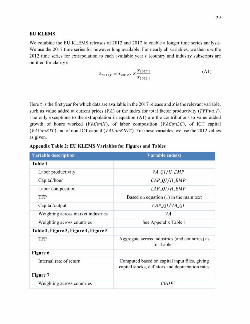
29

EU KLEMS

We combine the EU KLEMS releases of 2012 and 2017 to enable a longer time series analysis. We use the 2017 time series for however long available. For nearly all variables, we then use the 2012 time series for extrapolation to each available year 𝑡 (country and industry subscripts are omitted for clarity):

𝑥S()*+,! = 𝑥()*(,! ×𝑥()*+,-𝑥()*(,-

(A1)

Here 𝜏 is the first year for which data are available in the 2017 release and 𝑥 is the relevant variable, such as value added at current prices (𝑉𝐴) or the index for total factor productivity (𝑇𝐹𝑃𝑣𝑎_𝐼). The only exceptions to the extrapolation in equation (A1) are the contributions to value added growth of hours worked (𝑉𝐴𝐶𝑜𝑛𝐻), of labor composition (𝑉𝐴𝐶𝑜𝑛𝐿𝐶), of ICT capital (𝑉𝐴𝐶𝑜𝑛𝐾𝐼𝑇) and of non-ICT capital (𝑉𝐴𝐶𝑜𝑛𝐾𝑁𝐼𝑇). For these variables, we use the 2012 values as given.

Appendix Table 2: EU KLEMS Variables for Figures and Tables

Variable description Variable code(s)

Table 1

Labor productivity 𝑉𝐴_𝑄𝐼 𝐻_𝐸𝑀𝑃⁄

Capital/hour 𝐶𝐴𝑃_𝑄𝐼 𝐻_𝐸𝑀𝑃⁄

Labor composition 𝐿𝐴𝐵_𝑄𝐼 𝐻_𝐸𝑀𝑃⁄

TFP Based on equation (1) in the main text

Capital/output 𝐶𝐴𝑃_𝑄𝐼 𝑉𝐴_𝑄𝐼⁄

Weighting across market industries 𝑉𝐴

Weighting across countries See Appendix Table 1

Table 2, Figure 3, Figure 4, Figure 5

TFP Aggregate across industries (and countries) as for Table 1

Figure 6

Internal rate of return Computed based on capital input files, giving capital stocks, deflators and depreciation rates

Figure 7

Weighting across countries 𝐶𝐺𝐷𝑃"

30

Appendix Table 3. Alternative datasets for growth accounts in Europe

Notes: Sample periods and countries differ slightly across datasets.

EU KLEMS Total Economy (combination of 2012 and 2017 version)1985-95 1995-07 2007-15 1995-00 2000-07 2007-11 2011-15

(1) Labour productivity growth 2.18 1.41 0.45 1.64 1.25 0.35 0.54

Accounting decomp. 1 (p.p. contributions):(2) Capital/hour 1.14 0.80 0.43 0.94 0.70 0.61 0.26

(3) Labour composition 0.38 0.20 0.26 0.25 0.16 0.31 0.21

(4) TFP growth 0.65 0.42 -0.23 0.45 0.40 -0.57 0.10

Accounting decomp. 2 (p.p. contributions):(5) Capital/output 0.62 0.46 0.43 0.56 0.39 0.77 0.10

(6) Labour composition 0.57 0.31 0.40 0.39 0.25 0.48 0.32

(7) TFP growth 0.98 0.66 -0.37 0.70 0.62 -0.90 0.16

OECD1985-95 1995-07 2007-17 1995-00 2000-07 2007-11 2011-17

(1) Labour productivity growth 2.04 1.61 0.60 1.82 1.45 0.36 0.76

Accounting decomp. 1 (p.p. contributions):(2) Capital/hour 1.01 0.72 0.50 0.75 0.70 0.72 0.35

(3) Labour composition n.a. n.a. n.a. n.a. n.a. n.a. n.a.(4) TFP growth 1.01 0.86 0.06 1.03 0.74 -0.48 0.41

Accounting decomp. 2 (p.p. contributions):(5) Capital/output 0.60 0.39 0.45 0.35 0.42 0.84 0.20

(6) Labour composition n.a. n.a. n.a. n.a. n.a. n.a. n.a.(7) TFP growth 1.42 1.17 0.08 1.41 1.00 -0.65 0.57

Total Economy Database (April 2019)1990-95 1995-07 2007-17 1995-00 2000-07 2007-11 2011-17

(1) Labour productivity growth 2.48 1.49 0.56 1.76 1.30 0.41 0.66

Accounting decomp. 1 (p.p. contributions):(2) Capital/hour 1.34 0.82 0.61 0.78 0.85 0.98 0.37

(3) Labour composition 0.28 0.26 0.25 0.32 0.22 0.33 0.19

(4) TFP growth 0.88 0.42 -0.31 0.68 0.24 -0.91 0.09

Accounting decomp. 2 (p.p. contributions):(5) Capital/output 0.60 0.34 0.65 0.09 0.52 1.42 0.13

(6) Labour composition 0.46 0.45 0.43 0.54 0.38 0.58 0.34

(7) TFP growth 1.47 0.72 -0.54 1.16 0.41 -1.59 0.17

31

Appendix Table 4. EU KLEMS 2019 (with and without additional intangibles)

Notes: Source is Stehrer et al. (2019). Data start in 1995. Top panel includes only national accounts intangibles in output and capital and is from the “statistical” tables. Bottom panel includes additional intangibles and is from the “analytical” tables.

(2) (3) (4) (5) (6) (7)

1995-07 2007-17 1995-00 2000-07 2007-11 2011-17EU KLEMS Total Economy (2019 version, only NA intangibles)(1) Labour productivity growth 1.46 0.55 1.71 1.29 0.42 0.64

Accounting decomp. 1 (p.p. contributions):(2) Capital/hour 0.41 0.27 0.44 0.38 0.51 0.11

(3) Labour composition 0.19 0.21 0.24 0.16 0.26 0.17

(4) TFP growth 0.87 0.07 1.03 0.76 -0.36 0.36

Accounting decomp. 2 (p.p. contributions):(5) Capital/output -0.13 0.13 -0.19 -0.09 0.57 -0.17

(6) Labour composition 0.28 0.31 0.36 0.23 0.40 0.26

(7) TFP growth 1.32 0.11 1.55 1.16 -0.55 0.55

EU KLEMS Total Economy (2019 version, including additional intangibles)(1) Labour productivity growth 1.52 0.57 1.77 1.33 0.40 0.69

Accounting decomp. 1 (p.p. contributions):(2) Capital/hour 0.41 0.28 0.43 0.39 0.51 0.13

(3) Labour composition 0.19 0.21 0.24 0.16 0.26 0.17

(4) TFP growth 0.92 0.08 1.11 0.79 -0.37 0.38

Accounting decomp. 2 (p.p. contributions):(5) Capital/output -0.16 0.14 -0.24 -0.10 0.58 -0.16

(6) Labour composition 0.28 0.31 0.36 0.23 0.40 0.26

(7) TFP growth 1.40 0.12 1.67 1.21 -0.58 0.59

32

Table 1: Growth Accounting Across Datasets (percent or percentage points per year)

Notes: All data are Törnquist aggregates across individual countries. See the text for the expressions shown in lines 2 through 7. Penn World Tables aggregates the 15 countries that were members of the European Union before 2004; see notes to Figure 1 for the list. Because of data availability, EU KLEMS includes eight countries with complete growth-accounting data back to 1985. EU KLEMS ends in 2015, whereas PWT ends in 2017. See the data appendix for further details. The text explains the two accounting decompositions.

Penn World Table (version 9.1)(1) (2) (3) (4) (5) (6) (7)

1985-95 1995-07 2007-17 1995-00 2000-07 2007-11 2011-17

(1) Labour productivity growth 2.48 1.50 0.68 1.74 1.33 0.34 0.91Accounting decomp. 1 (p.p. contributions):

(2) Capital/hour 1.09 0.72 0.55 0.73 0.72 0.80 0.39(3) Labour composition 0.44 0.32 0.25 0.35 0.29 0.28 0.22(4) TFP growth 0.95 0.47 -0.12 0.67 0.32 -0.74 0.30

Accounting decomp. 2 (p.p. contributions):(5) Capital/output 0.21 0.19 0.45 0.04 0.29 1.11 0.01(6) Labour composition 0.72 0.53 0.42 0.58 0.50 0.48 0.38(7) TFP growth 1.55 0.78 -0.19 1.12 0.54 -1.25 0.52

EU KLEMS Market Sector (combination of 2012 and 2017 version)

1985-95 1995-07 2007-15 1995-00 2000-07 2007-11 2011-15

(1) Labour productivity growth 2.41 1.66 0.42 1.84 1.53 0.15 0.69Accounting decomp. 1 (p.p. contributions):

(2) Capital/hour 1.11 0.88 0.45 1.05 0.76 0.63 0.26(3) Labour composition 0.37 0.20 0.30 0.19 0.20 0.33 0.27(4) TFP growth 0.93 0.65 -0.30 0.73 0.60 -0.78 0.19

Accounting decomp. 2 (p.p. contributions):(5) Capital/output 0.56 0.51 0.48 0.69 0.39 0.88 0.08(6) Labour composition 0.53 0.29 0.43 0.28 0.29 0.48 0.38(7) TFP growth 1.33 0.96 -0.45 1.06 0.89 -1.16 0.27

33

Table 2: Tests for Breaks in Market-Sector TFP Growth, 1980-2015

Notes: First set of numbers for each country or region are p-values against the null of a constant mean and are heteroskedasticity and autocorrelation robust. Second set of numbers are estimated dates after which the mean changes. TFP growth is annual data for the market-sector from the 2012 and 2017 EU KLEMS datasets. For estimation details of the Quandt tests, see Fernald, Hall, Stock, and Watson (2017).

Chow test for break Chow test for break after 2007 relative to U.S. after 2007

Country 1 break 2 breaks

United States 0.40 0.51 0.252006 1998 2005

Europe 0.10 0.33 0.03 0.432007 1990 2007

Northern Europe 0.05 0.21 0.01 0.252007 1991 2007

Southern Europe (Italy, Spain) 0.20 0.28 0.22 0.941995 2000 2009

Germany 0.27 0.16 0.23 0.672007 2001 2009

France 0.09 0.24 0.00 0.112000 1989 2007

Netherlands 0.55 0.25 0.19 0.882007 1999 2007

United Kingdom 0.13 0.27 0.01 0.162007 1987 2007

Spain 0.10 0.31 0.42 0.801988 1988 2009

Italy 0.40 0.33 0.29 0.882000 2000 2009

(Sup Wald) TestQuant Likelihood Ratio

34

Figure 1: European total factor productivity growth: A long downward trend

Notes: Source is PWT 9.1 (Feenstra, Inklaar, and Timmer, 2015). The solid line is European TFP growth, defined as a Törnquist index of TFP growth for 15 countries that were members of the European Union before 2004. Country TFP is variable RTPNA, and weights are nominal PPP-adjusted GDP, variable CGDPO. Countries are Austria, Belgium, Denmark, Finland, France, Germany, Greece, Ireland, Italy, Luxembourg, Netherlands, Portugal, Spain, Sweden, and the United Kingdom. The red dashed line is biweight trend with bandwidth of 12 years. The maroon dashed line that diverges from the red line after the late 1990s, and ends in 2007, is the estimated trend using data through 2007 only.

2007

-4-2

02

4An

nual

per

cent

cha

nge

1950 1960 1970 1980 1990 2000 2010 2020year

European TFP (1955-2017)

35

Figure 2A. Capital-output ratio not falling short of trend

Figure 2B: Investment share fell after the recession

DEU

ESP

FRA

GBR

ITA

DEU

ESP

FRAGBR

ITA

DEU

ESP

FRA

GBR

ITA

2007

.91

1.1

1.2

2007

=1

1990 2000 2010 2020Source: Penn World Table 9.1 (Feenstra, Inklaar and Timmer, AER 2015), variables RKNA and RGDPNA.Notes: Figure shows the capital-output ratio in the EU-15 for 1990–2017 and for France (FRA),Germany (DEU), Italy (ITA), Spain (ESP) and United Kingdom (GBR) the values in 1990, 2000and 2017. The capital-output index is normalised to 2007=1.

2007

.18

.2.2

2.2

4.2

6N

omin

al ra

tio o

f inv

estm

ent t

o G

DP

1970 1980 1990 2000 2010 2020Source: Penn World Table 9.1 (Feenstra, Inklaar and Timmer, AER 2015).Notes: Nominal gross fixed capital formation relative to nominal GDP for the 15 original EU membercountries.

36

Figure 3. Slower frontier TFP growth and divergence

Source: Market-sector TFP growth from EU KLEMS 2017, combined with EU KLEMS 2012 (before 1995). PPP-adjusted TFP levels are based on Inklaar-Timmer (2009) for 1997.

UnitedStates

NorthernEurope

SouthernEurope

Austria

.6

.7

.8

.9

1

1.1

1.2U

SA in

199

5=1

1985 1990 1995 2000 2005 2010 2015North: Belgium, Finland, France, Germany, Netherlands, UKSouth: Italy, Spain

37

Figure 4. Since 2007, anemic TFP growth is the new normal

-10

12

Aver

age

annu

al p

rodu

ctiv

ity g

row

th (%

)

Spain ItalyGermany

BelgiumDenmark

France

NetherlandsAustria

United States

United KingdomSweden

Finland

1995–2007

-10

12

Aver

age

annu

al p

rodu

ctiv

ity g

row

th (%

)

FinlandFrance

Sweden Italy Spain

United KingdomDenmark

AustriaGermany

NetherlandsBelgium

United States

2007–2015ICT sectorMarket servicesBubble sectorsNon-IT manufacturingOther industries

Source: EU KLEMS 2017.Notes: ICT sector covers ICT goods and services, Bubble sectors are finance and construction, Other industries are agriculture, mining and utilities.

38

Figure 5. TFP fell in 2009, rebounded in 2010

-8

-6

-4

-2

0

2

4

6A

nnua

l gro

wth

(in

%)

1985 1990 1995 2000 2005 2010 2015Source: EU KLEMS 2017, combined with EU KLEMS 2012.Notes: The solid line shows GDP-weighted average market economy TFP growth for Austria, Belgium,Finland, France, Germany, Italy, Spain, Netherlands and United Kingdom. The shaded area spans the minimum and maximum growth rate observed in each year in this set of countries.

39

Figure 6. Market power: increase in apparent profits in many countries

-.05

0.0

5.1

.15

-.05

0.0

5.1

.15

1995 2000 2005 2010 2015 1995 2000 2005 2010 2015 1995 2000 2005 2010 2015 1995 2000 2005 2010 2015 1995 2000 2005 2010 2015

Austria Denmark Finland France Germany

Italy Netherlands Spain Sweden United Kingdom

Source: IRR: EU KLEMS 2017, calculations by Daan Freeman. Government bond yields: ECBNotes: Figure shows for each country the internal rate of retun on fixed assets minus the 10-year government bond yield.

40

Figure 7. Steady rise in intangible investment

United States

Europe

05

1015

20%

of M

arke

t eco

nom

y va

lue

adde

d

1995 2000 2005 2010 2015 2020Source: INTAN-Invest Database, January 2019, Corrado et al. (2016).Notes: European countries covered are Austria, Belgium, Denmark, Finland, France, Germany, Greece, Ireland, Italy,Luxembourg, Netherlands, Portugal, Spain, Sweden and UK. Red area indicates the range of investment rates and thesolid red line is the weighted average European productivity level. Ireland is omitted from the European range asits R&D investment increased by a factor of 5.5 between 2014 and 2016, leading to an investment rate of 31 percent in that year. Eurostat investment data show the data return to below their 2015 level by 2018.