DI

SC

US

SI

ON

P

AP

ER

S

ER

IE

S

Forschungsinstitut zur Zukunft der ArbeitInstitute for the Study of Labor

Does Confl ict Disrupt Growth?Evidence of the Relationship between Political Instability and National Economic Performance

IZA DP No. 4762

February 2010

Solomon W. PolachekDaria Sevastianova

Does Conflict Disrupt Growth? Evidence of the Relationship between

Political Instability and National Economic Performance

Solomon W. Polachek State University of New York at Binghamton

and IZA

Daria Sevastianova University of Southern Indiana

Discussion Paper No. 4762 February 2010

IZA

P.O. Box 7240 53072 Bonn

Germany

Phone: +49-228-3894-0 Fax: +49-228-3894-180

E-mail: iza@iza.org

Any opinions expressed here are those of the author(s) and not those of IZA. Research published in this series may include views on policy, but the institute itself takes no institutional policy positions. The Institute for the Study of Labor (IZA) in Bonn is a local and virtual international research center and a place of communication between science, politics and business. IZA is an independent nonprofit organization supported by Deutsche Post Foundation. The center is associated with the University of Bonn and offers a stimulating research environment through its international network, workshops and conferences, data service, project support, research visits and doctoral program. IZA engages in (i) original and internationally competitive research in all fields of labor economics, (ii) development of policy concepts, and (iii) dissemination of research results and concepts to the interested public. IZA Discussion Papers often represent preliminary work and are circulated to encourage discussion. Citation of such a paper should account for its provisional character. A revised version may be available directly from the author.

IZA Discussion Paper No. 4762 February 2010

ABSTRACT

Does Conflict Disrupt Growth? Evidence of the Relationship between Political Instability and National Economic Performance* Current empirical growth models limit the determinants of country growth to geographic, economic, and institutional variables. This study draws on conflict variables from the Correlates of War (COW) project to ask a critical question: How do different types of conflict affect country growth rates? It finds that wars slow the economy. Estimates indicate that civil war reduces annual growth by .01 to .13 percentage points, and high-intensity interstate conflict reduces annual growth by .18 to 2.77 percentage points. On the other hand, low-intensity conflict slows growth much less than high-intensity conflict, and may slightly increase it. The detrimental effect of conflict on growth is intensified when examining non-democracies, low income countries, and countries in Africa. JEL Classification: C2, O1, O47, O57, P47, P52 Keywords: economic growth, war, conflict Corresponding author: Solomon W. Polachek Department of Economics and Department of Political Science State University of New York at Binghamton Binghamton, New York 13902-6000 USA E-mail: polachek@binghamton.edu

* We thank Christopher Hanes, John Lott, David Clark, Luis Locay, Michael Intriligator, and Carlos Seiglie for their helpful comments and suggestions. Versions of this paper were presented at the Peace Science Society Conference (Columbia, SC, November 2007), the American Economics Association Conference (New Orleans, LA, January 2008), International Studies Association Conference (San Francisco, CA, March 2008), and Eastern Economic Association Conference (New York, NY 2009).

1

Does Conflict Disrupt Growth? Evidence of the Relationship between

Political Instability and National Economic Performance

From 1899 to 2001, there have been over 200 wars throughout the world. In 2007

alone, there were 14 active armed conflicts.2 One important question is how wars affect a

country‟s economic well-being. Indeed the depletion of resources during wars may be

one reason why some countries fail to sustain adequate economic growth. Because

economic growth affects a population‟s well-being, this question concerning how war

relates to growth is important from a policy perspective. Overall economic theory is

ambiguous about the relationship between war and economic growth. On the one hand,

war destroys capital and utilizes manpower. On the other, war mobilizes the workforce,

increasing effort and enhancing productivity.

This paper utilizes various measures of interstate and intrastate conflict from the

political science literature to ascertain how a nation‟s involvement in international and

civil wars relates to its economic growth. To get at these measures the paper utilizes

techniques from the economics growth theory literature, which at least since the 1990s

turned empirical. Our innovations over past research are to use far longer time-series data

on country growth, to incorporate detailed information on both domestic and international

conflict, to include conflict duration and severity, to examine various country

subsamples, and to adopt fixed-effects estimation techniques.

Empirical growth models estimate how changes in a country‟s physical and

human capital as well as technology enhance GNP per capita. For example, Barro (1991)

and Sachs and Warner (1997) find that a tropical geography and an abundance of natural

resources are negatively related to growth.3 Trade liberalization, democracy, government

stability, and a legal system that strongly protects private property rights enhance

2 SIPRI Yearbook 2008.

3 Mehlum, H. et. al (2006) argue that institutions are a key determinant of long run economic growth.

2

growth.4 One particular innovation of this literature was to examine how government and

economic structure affect growth. As such, Londregan and Poole (1990), Barro (1991),

Barro and Lee (1993), Easterly et al. (1993), Easterly and Rebelo (1993), Alesina and

Perotti (1996), Persson and Tabellini (2006) find that government and social instability

and political violence often negatively affect growth.

At about the same time the growth literature evolved, political scientists began to

apply quantitative methods to classify and measure political interactions including

interstate and intrastate wars. Early compilations of wars and their associated casualties

(Wright (1942) and Richardson (1960)) code wars that have taken place well before

accurate national accounts data were available to assess their economic impact.

Nowadays there are two main ongoing compilations of war that do not have this

deficiency because they are more current (1) Uppsala University Data on Armed Conflict

compiled by The Centre for the Study of Civil War at the International Peace Research

Institute, Oslo (PRIO) and Uppsala Conflict Data Program (UCDP) at the Department of

Peace and Conflict Research, and (2) the Correlates of War (COW) project originally

compiled by J. David Singer at the University of Michigan. These data are periodically

updated, the latter by the Peace Science Society (PSS), and contain detailed information

on fatalities and duration of both international and civil wars for the years 1970-2000,

which include and go beyond the years analyzed by Barro and Sachs-Warner in their

analyses of growth.

At least from a policy perspective, it is important to measure how such fighting

within and between countries affects a country‟s economic growth. Because wars have

not stopped, the relevance of this question persists. The estimates obtained in this paper

hopefully can be used to assess how wars could affect future world growth.

We find that interstate conflict decreases economic growth by .18 to 2.77

percentage points, while intrastate conflict decreases economic growth by .01 to .13

4 Some of the recent literature on democracy finds the link between regime type, income, and religion.

Specifically, Borooah, and Paldam, (2007) find that poverty, Communism, and Muslim culture are the main

barriers to democratic governance.

3

percentage points. Such negative growth intensifies with conflict severity. Furthermore,

conflict reduces economic growth the most in the short run, whereas in the long run

economies recover from the adverse effects of wars. Our results show that poor countries

engage in civil wars, while rich countries engage in international wars. Civil wars hurt

economic prospects of all affected countries, and are especially detrimental to economic

growth in non-democracies. International wars reduce growth most in African and low-

income countries. Interestingly, international conflict waged by the OPEC members

augments rather than reduces growth. Overall, the impact of conflict varies with conflict

intensity, as well as by country type, wealth, and polity.

We approach our analysis in five steps. First, we replicate and extend the Barro

growth model with updated Sachs-Warner variables calculated from the Penn World

Tables (Version 6.1 dated 2000), the World Development Indicators (2005), and the

Political Risk Services Group IRIS-3 data. Second, we introduce Correlates of War

(COW) measures of interstate and intrastate conflict by utilizing both duration and

severity measures. Third, we examine smaller time intervals. Fourth, we divide countries

by region, polity, and income level to examine the effects of wars separately in each of

those groups. Finally, fifth, we corroborate our results using an alternative empirical

specification.

II. Brief Literature Review

Robert Solow‟s (1957) path breaking innovation was to couch economic growth

within a neoclassical framework. This framework significantly advanced the prior more

rigid Harrod-Domar fixed proportions model developed in the 1930s, and led to

influential empirical work by Barro (1991), Sachs-Warner (1995,1997) and others5.

Though not the main focus, Barro (1991) incorporates two measures of political

instability. Both of these, the number of revolutions and or coups per year (see Barro

5 Most prominent work in growth literature includes done by Barro (1989, 1991), Barro and Sala-i-Martin

(1992, 1995), Barro and Lee (1993), Mankiw, Romer, Weil (1992), Sachs and Warner (1995, 1997), and

Hall and Jones(1997,1999).

4

andWolf 1989) as well as the number of political assassinations per year per million

population negatively affects growth.6 Barro‟s interpretation is that both of these

variables distort property rights, and thereby hamper investment and decrease growth.

Barro and Lee (1993) subsequently confirm that revolutions inhibit growth as do Knack

and Keefer (1995) and Easterly and Levine (1997). Alesina et al. (1996) similarly

obtained a negative coefficient on the probability of government change in a growth

regression. Furthermore, Alesina and Perotti (1996) confirmed that political violence

(assassinations, deaths from political violence, coups, and a dictatorship dummy) reduces

growth. In recent line of literature, Jong-A-Pin (2009) finds only the instability of the

political regime has a robust and significant negative effect on economic growth. In

contrast Barro and Lee (1993) found no significant relationship between political

violence measured by a war dummy and growth. Similarly, Easterly et al. (1993) and

Easterly and Rebelo (1993) established that assassinations, coups, revolutions, and war

casualties variables have no significant effect on economic growth.7 In addition, a meta-

study by Brunetti (1997), indicates most analyses yield a negative but insignificant

political violence growth relationship. In sum, these studies lack robustness regarding the

effects of political instability.

More recently, some studies adopt growth theory to examine the economic effects

of civil wars, but to date none to our knowledge adequately incorporate international

wars. This literature points to various theoretical reasons why civil wars are detrimental

to the steady state long run income per capita growth rate.8 These include the effects of

declines in human and physical capital, the growth of labor, and reductions in trade and

FDI. War also creates uncertainty and disrupts daily market activity. In long run models,

studies find weak effects of civil wars on growth. Models of civil wars using spatial

econometric techniques to get at spillovers better capture the destructive influence on

both home and neighboring territories. Because these effects are better captured with 5-

year intervals, Murdoch and Sandler (2004) conclude that the devastating effects of civil

6 Barro (1991) obtaines hiw two measures from Banks (1979). Some studies also used political freedom

and civil liberties measures from Gastil (1989). 7 Easterly and Rebelo (1993) find a negative coefficient on casualties only when marginal tax rates are

included in the specification. 8 Sambanis (2001), Collier and Sambanis (2002), Murdoch and Sandler (2002, 2004).

5

wars are generally short lived, but they do not examine these duration effects for

interstate wars. In addition, Collier and Sambanis (2002) find that civil wars are rare in

democracies, as most democracies also happen to be high-income countries with low

civil war incidence. Hillman (2009, chapter 3) explains the different propensities

democracies and autocracies engage in war by the costs of war for the general population

and the personal benefits for autocratic rulers.While these studies recognize the

complexity of causes of civil war, which possibly helps explain the difference in their

economic effects, it is beyond the scope of this paper to distinguish between various

types of civil war, such as war based on ethno-linguistic division vs. rent-seeking and

resource extraction, for example. The paper in part accounts for that by examining

regional differences, as those frequently act as a proxy for civil war type.

Contemporary growth studies have also given much attention to conflict in Sub-

Saharan Africa. For example, Merrouche (2008) argues that de-mining programs in

Mozambique have generated positive economic effects. Another line of literature stresses

the importance of neighborhood effects in Africa (including Brock and Durlauf, 2003).

Research on the effects of ethnic heterogeneity on civil war in Africa has also shed light

on the mechanisms underlying war incidence.9Finally, current research has addressed the

question of conflict trap. In his book The Bottom Billion, Collier writes about the civil

war trap, where past civil war increases the probability of future civil war. In such

environments, negative association between civil war and growth is self-perpetuating.

A number of deficiencies remain in assessing these studies. First, none of these

studies comprehensively examine the effect of international wars on growth. Second,

most analyses of the effects of conflict on growth stop at or before the 1990s. Third, not

all studies use actual war data. Those that do fail to take account of war severity. Fourth,

with the exception of several studies pertaining to the effects of civil wars, most use 30-

year time durations. But as Murdoch and Sandler (2004) show, the effects of civil wars

can be short-lived, implying the necessity to evaluate the time duration over which

growth can be affected. Fifth, virtually all the studies that measure the effects of conflict

9 Alesina, et al. (2003&2006), Montalvo and Reynal-Querol (2005).

6

on growth fail to examine interactive effects. They look at how conflict relates to growth

holding constant such variables as region, polity and country income, but not whether

wars have a more detrimental effect in Africa or America, or whether democracies suffer

more than autocracies. Finally, each study adopts the Barro (1991) and Sachs-Warner

(1995, 1997) specification without checking robustness using alternative statistical

specifications. As already mentioned in the last section, we overcome these shortcomings

first by utilizing data through 2000; second, by using detailed interstate and intrastate war

data encompassing both war incidence and severity; third, by analyzing various time

durations of the effects of wars from one to thirty years; fourth, by stratifying by region,

polity, and country income to get at wars‟ interactive effects; and finally fifth, by using

an alternative statistical specification to corroborate our results. Unlike the studies which

utilize cross-sectional Barro style regressions, we incorporate statistical models making

use of within country fixed effects.

The mechanism through which conflict operates is not a subject of this paper.

However, the literature contains a number of themes. For example, both Persson and

Svensson (1989) and Tabellini and Alesina (1989) argue that governments of politically

unstable or violent countries are more prone to rent-seeking, and therefore adopt

suboptimal policies on taxation, as well as face higher debt and government consumption

to GDP ratios. Research published in Forty Years of Research on Rent Seeking, Volume

II, Applications: Rent Seeking in Practice, Congleton, et. al (2008) addresses the linkage

between rent-seeking and economic growth and development. As rent-seeking is

typically considered a deadweight loss to society, conflict which encourages rent-seeking

would also be associated with fewer property rights and a poorer rule of law. Fewer

property rights would decrease growth rates and cause a lower steady state income level,

thereby reducing long run growth prospects.10

As North (1990, p.54) puts it, “the inability

of societies to develop effective, low-cost enforcement of contracts is the most important

source of both historical stagnation and contemporary underdevelopment in the Third

World.” Hillman (2004) shows how absence of the rule of law allows the strong to

10

Persson and Svensson (1989) and Tabellini and Alesina (1989).

7

exploit the weak and how the disincentives confronting the weak underlie development

failure.

Similarly, uncertainty about property rights brought about by conflict can distort

investment and saving incentives. This research reveals that in the face of uncertainty and

weak property rights actors defer making investments especially when they cannot

completely recover their sunk costs. These in effect create a tax on investment and

hamper long term growth.11

In addition, instability impedes savings incentives and

therefore lowers economic growth.12

Also, if wars slow political and economic reforms

needed in an economy, long run income growth can be weakened by the economy‟s

failure to adapt to change.13

Another recent line of empirical growth literature examines how conflict affects

the allocation of international aid by donors. For example, Chauvet (2003) argues that

while violent instability attracts foreign aid, social instability discourages it. Therefore, to

the extent that aid stimulates economic growth, conflict might affect aid allocation

decisions and therefore growth rates in aid recipient countries.14

In addition, economic research paid much attention to the conflict-trade

relationship. Notably, Polachek (1980, 1997) argues that trade reduces conflict. In this

context, simultaneous equations models do not alter this finding, but actually corroborate

it. While we acknowledge the importance of inclusion of trade in modeling the conflict-

growth relationship, a simultaneous equations approach is beyond the scope of the

current study, although it does pose a productive future venue in the study of conflict.

Authors also acknowledge that trade might have a differential impact on the economy

depending on the type of country: for example, in the Southeast Asian country grouping

much of the rapid growth has been propelled by increased trade and FDI, unlike Latin

American countries who experienced a smaller rate of trade growth; OPEC countries

11

Dixit and Pindyck (1994); Aizenman and Marion (1993); Alesina and Perotti (1996). 12

Venieris and Gupta (1986). 13

Dollar and Svensson (2000). 14

In research on allocation of foreign aid, a meta-study by Doucouliagos, H. and M. Paldam (2008)

establishes that neither good policy nor aid itself are significant factors.

8

have traded primarily in oil exports, and African countries have remained heavily

dependent on primary product exports.

III. The Model

In line with Mankiw, Romer, and Weil (1992) interpretation of the Solow (1957)

growth accounting framework, the estimating equation is expressed as a growth rate, or

the time-difference between natural logs of income per worker at the end (Yit) and

starting points (Yio) of a given time period. If the speed of convergence to the steady state

y* at time t from the initial value of income is λ, then the growth rate during the transition

to the steady state is expressed as:

ln yt – ln y0 = (1-e-λt)lny* - (1-e-λt)lny0. (1)

based on specifying country output as a Cobb-Douglas production function and making a

series of substitutions for the steady state. This yields the following estimating equation

for growth of income per capita:15

ln yt – ln y0 = a + (1-e-λt)[α/(1-α-β)]ln(sk) + (1-e-λt)[β/(1-α-β)]ln(sh) –

(1-e-λt)[(α+β)/(1-α-β)]ln(n+g+δ) – (1-e-λt)lny0 + ε, (2)

where a is a constant; α and β are the elasticities of output with respect to physical and

human capital, and 1-α-β is the output elasticity of effective units of labor; sk and sh

denote the savings rates of physical and human capital respectively; n is the rate of

population growth, g is the rate of technological progress, and δ is capital depreciation;

and finally ε is a country specific random error. The last term with lagged income shows

negative coefficient, otherwise known as the convergence parameter, which signifies that

given identical production functions, a country with a lower initial income level will

15

Derivation of y* is as follows. The transition equations for human and physical capital are given by

dk/dt = sky – (n+g+δ)k and dh/dt = shy – (n+g+δ)h. Taking logs and substituting for the steady state values

of capital (i.e. when dk/dt = 0 and dh/dt =0) into the production function Yt = KtαHt

β(AtLt)

1-α-β, where α + β

<1 yields the following steady state income per capita equation: ln[Yt/Lt] = lnA0 + gt + [α/(1-α-β)]ln(sk) +

[β/(1-α-β)]ln(sh) – [(α+β)/(1-α-β)]ln(n+g +δ). If A0 = a + ε, where a is a constant and ε is a country specific

shock, while ignoring gt, steady state income per capita y* will be: y* = ln[Y/L] = a + [α/(1-α-β)]ln(sk) +

[β/(1-α-β)]ln(sh) – [(α+β)/(1-α-β)]ln(n+g+δ) + ε.

9

grow faster.16

This term is peculiar to the growth rate equation (1), and is not observed in

the steady state income level equation.

In the empirical growth literature, several specifications are used to decompose

income into economic inputs. One possible specification describes the steady state level

of income per capita where income in the last period is at the steady state level, while

other specifications look at the growth rate of income per capita, as the economy moves

from the first period to the last, which captures transition to the steady state. 17

The long

term framework – whether it examines the level of steady state income or the average

growth rate of income over the entire period – underlies cross-sectional studies.

Conversely, a panel framework considers growth rates over several shorter time durations

and thus models growth in the short run. Because in such studies the notion of the steady

state is absent, they are referred to as “growth regressions”. In these studies, the main

impact of war is the destruction of existing physical capital and the temporary reduction

of human capital accumulation. The models also predict a burst of post-war growth as the

economy recovers, or returns to its steady state path.

IV. The Data

We use seven data sources: (1) Penn World Tables, (2) World Bank data, (3) Sachs

and Warner data, (4) International Risk Investment Survey (IRIS) data, (5) United States

Central Intelligence Agency (CIA) World Factbook data, (6) Polity IV data, and (7)

Correlates of War (COW) data. We discuss the first five only briefly because they are

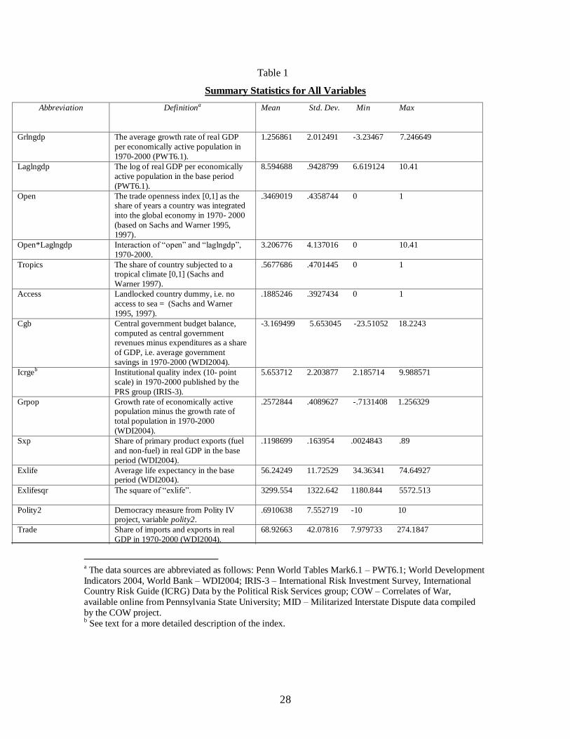
familiar to many economists, and then concentrate on the latter two. A summary of all

variables is contained in Table 1.

17

The dependent variable in growth regressions is usually the average growth rate, i.e. the logarithm of the

ratio of the last period income to the base period income divided by the number of years within the period. 17

The dependent variable in growth regressions is usually the average growth rate, i.e. the logarithm of the

ratio of the last period income to the base period income divided by the number of years within the period.

10

The Penn World Table (PWT) provides economic time series data for 188

countries.18 Data are denominated using a common set of prices so that real quantity

comparisons can be made. We use this data set to obtain information on GDP and GDP per

capita. The World Development Indicators (WDI) contains more than 900 indicators on over

200 economies. The data are based on censuses and household surveys drawn in conjunction

with numerous international, government, and nongovernmental organizations. Sources used

are the most authoritative available, and in reporting these data the World Bank made

considerable effort to standardize the information. We use the WDI to obtain information on

government revenues and expenditures, primary product exports, population growth and life

expectancy. The IRIS data are based on information obtained from the International Country

Risk Guide. It contains statistics on corruption in government, rule of law, bureaucratic

quality, ethnic tensions, repudiation of contracts by government, and risk of expropriation.

We utilize data containing a ten-point index of each country‟s institutional quality. The CIA

World Fact- book is an annual volume containing information on land, water, people,

government, economy, communications, and defense forces. It began annual publication in

1981 and contains statistics on 165 nations. We utilize access to sea to update the

“landlocked” variable in the replication Sachs and Warner (1997) specification, as well as

information on political regime and economic policy to update the “openness to trade

variable”.

The Polity IV and the Correlates of War data are put together by political scientists.

Polity IV was originally begun by Ted Gurr of the University of Maryland's Center for

International Development and Conflict Management. It now is continued under the auspices

of Monty G. Marshall and Keith Jaggers at the George Mason University's Center for Global

Policy. It contains coded annual information on regime and authority characteristics for all

independent states with a population greater than 500,000 over the years 1800-2004. The

degree of democracy is coded on a ten-point scale as is the degree of autocracy. The

combination yields a democracy score between -10 and 10. We use this variable to stratify

between democratic and non-democratic countries.

18

Our sample does not include states formed upon brake-ups: for example, Yugoslavia in the 1990s or the

formerly Socialist nations which joined state membership upon the break-up of the Eastern bloc. Data

availability for such countries is often limited, with the time-series only beginning in the early 1990s.

11

The Correlates of War Data began in 1963 as a compilation of wars by J. David

Singer, a political scientist at the University of Michigan. The data‟s objective has been the

systematic accumulation of information related to wars. The war data were first published in

Singer and Small (1972). In the late 1990s, the compilation was transferred to the Peace

Science Society (PSS) at the Pennsylvania State University. Currently, the various parts of

the COW data accumulation project are hosted by separate institutions that maintain and

update individual datasets.19 The data set contains information from 1816 to the present on

many attributes of international politics, particularly wars and militarized disputes, as

well as information on national capabilities. We utilize the war data as well as the

militarized interstate dispute data. The war data contain the following information for

each war: states involved, dates, duration, deaths, result, initiator state, area where the

event occurred. A war is a militarized dispute with at least 1,000 battle deaths per year.

The militarized interstate dispute (MIDs) data documents instances not requiring 1,000

battle deaths, when one state threatened, displayed, or used force against another in 1816-

2001. As with wars, the data report the states involved, the dates of each MID, and the

duration.20

A brief examination of data suggests, the relationship between conflict and per

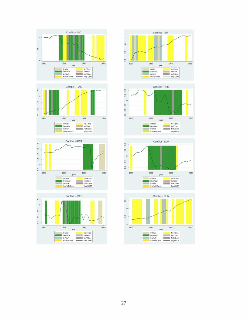
capita GDP is not straightforward. Figure 1 graphs annual real GDP per capita (measured

in logs) over the 1970-2000 time period for sixteen representative countries. The shaded

regions mark periods of war. These can be international interstate wars (beige), domestic

intrastate wars (green), militarized interstate disputes short of war (bright yellow), or

some combination, of which there are four possibilities: international wars and lower

MIDs (blue); international wars and civil wars (pink); lower MIDs and civil wars (grey);

international wars, lower MIDs, and civil wars (dark yellow). The un-shaded white

portion denotes peaceful years with zero conflict.

The examination of dyads involved in conflict reveals no particular regularities.

For example, one might suspect that such country pairings – especially in the post-WWII

19

Project History online: http://www.correlatesofwar.org/

20 The COW data enable us to discern not only between varying levels of conflict intensity, but to also

clearly establish the boundaries/succession of such events.

12

period – might involve a high-income and a low-income country engaged in international

strife. War summary statistics provided by the COW project indicate that only about a

third of dyads involved in international war after WWII were those where a rich country

fought a poor country, i.e. a substantial portion of international conflict, predominantly in

Africa and Latin America, is actually between low-income countries.21

No pattern emerges regarding whether one type conflict precedes or follows

another. Nor is it the case that the duration of one type conflict is related to the duration

of another. An increase in low-level conflict is not necessarily accompanied by an

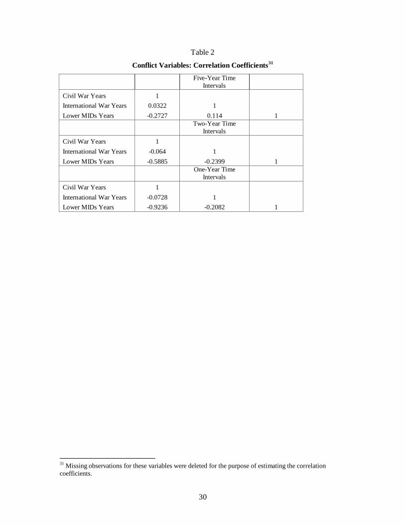
increase in either civil or international wars. To see this, Table 2 correlates the number of

years a nation engages in each type conflict. For the most part, the correlation coefficients

are negative. They are more negative the shorter the time interval, implying that nations

are less involved in both inter- and intrastate conflicts within short time periods.

Figure 1 also shows that neither international wars nor civil wars necessarily

reduce per capita income, and in fact can temporarily raise it. Similarly, in several

instances low-intensity conflict is associated with a rise in per capita income. Moreover,

it is not clear that one type of conflict need necessary precede or follow another. In

Rwanda, India, and Angola, for instance, low-level MIDs precede wars; but civil war in

Burundi precedes low-level MIDs. There are also several instances when low-intensity

conflict both precedes and follows wars, as in Chad, Uganda, and Nicaragua. On many

graphs, one can identify a decline in real income per capita preceding the onset of war,

and one can identify a period of recovery marked by per capita GDP growth following a

war. Examples of this would be the civil wars in Angola, Iran, Uganda, El Salvador, and

Chad. During war the per capita GDP appears to decline, but not necessarily so, as

evident in the examples of Angola, Iran, Israel, and Syria. For this reason a more detailed

multivariate approach is warranted.

21

Another interesting question is whether the relationship between conflict and growth depends

on a nation‟s winner or loser status in inter- or intra-state fighting. Although this paper does not incorporate

such a distinction, it does present interest as a future research venue.

13

V. Replication and Extension of the Sachs-Warner Model

Sachs and Warner (1997) examine growth from 1970-1990 by adapting the

following equation:

(lnY1990 – lnY1971)i = 0 + 1lnY1970i + ’2Zi + Ci + i (3)

The dependent variable is the average growth rate measured as real GDP per worker over

the entire period (normalized to annual rates by dividing by twenty, the number of years

the data span). The independent variables are initial GDP per economically active

population in 1970, openness to trade (using the Sachs and Warner (1995) openness

index, which accounts for both the volume of trade measured as the share of exports and

imports in GDP, and also for whether a country was under a socialist regime and engaged

in protectionism), an interaction variable for openness and initial income, the fraction of

the territory in the tropics, a landlocked dummy, central government budget balance,

institutional quality index, growth of the economically active population, the share of

primary product exports in GDP, the average life expectancy, and its square; and finally

Ci is the conflict variable measuring duration or severity of international and civil wars.

The unit of observation is a country denoted by i. To anchor our results to what has

already been done, we begin by replicating Sachs and Warner (1997) using a data set

extended to 2000 and then extending this replication further by adding war data.

The results are given in Table 3. The initial column contains the Sachs and

Warner 1970-1990 results. Column (1) is our replication using 1970-2000 data. As can be

seen the results are very similar to Sachs and Warner (1997). Columns (2) and (3) add

measures for interstate and intrastate wars. Adding data on wars does not change the

previous coefficients, but we find little effect of wars on growth, whether measured as the

proportion of years at war (rows 10-12), or battle deaths (rows 13-14). As will be

illustrated in the next section, examining growth over the entire 1970-2000 time period

might camouflage the effect of war, because the approach does not account for the

particular dates wars are fought within the thirty-year period. Possibly the negative

effects of a war fought late within the three decades (for example in the 1990s) might be

14

more important than a war fought early within the three decades, especially if the effects

of an earlier war dissipate when measured over the thirty-year time span. The Sachs and

Warner method does not take such time aspects into account.

VI. Estimation Issues

There are two issues regarding empirical estimation. First is to discern short-run

and long-run effects of wars. For this, we break up our observations on each country into

shorter intervals within the 1970-2000 time interval used by Sachs and Warner (1997). In

doing so, we use five-year time periods (1971-1975, 1976-1980, 1981-1985, etc.), then

we use two year time intervals (1971-1972, 1973-4, etc.), and finally one-year intervals.

As will be explained below, in each case we adopt cross-sectional and fixed-effect (FE)

estimation approaches.

Second is whether to focus on growth differences between war and non-warring

nations, or alternatively to focus on the effects of war and non-war periods within given

countries. The current empirical growth literature focuses on differences in growth

between countries. Such cross-sectional analysis cannot discern whether conflict deters

(or stimulates) growth, or instead whether low (or high) growth countries are simply

more prone to conflict because of their innate country attributes. One way to better isolate

the causal relationship is to examine whether growth changes within each country as

conflict levels change. To do this one can employ a fixed-effect (FE) regression model.

For this reason, we estimate a panel version of (2) where our units of observation are

country-specific short-run growth rates (computed over five-year periods, two-year

periods and computed annually).

Using a fixed effects regression is consistent with the neo-classical growth theory.

FE models assume each country has its own growth rate determined not only by the

exogenously given rates of savings, population growth, and technological progress, but

also by country-specific factors that capture the differences in preferences and

technology, and thus shape a unique growth path to the steady state. While the neo-

15

classical growth framework implies an identical aggregate production function for all

countries, introducing fixed effects allows for country-specific effects, where the

aggregate production function can vary across countries.

Approximating around the steady state, the growth equation can be rewritten as:

lnytj = (1 – e-λτ

) [α/(1-α)]ln(s) - (1 – e-λτ

) [α/(1-α)]ln(n + g + δ) + e-λτ

lnytj-1

+ (1 – e-λτ

) lnA0 + g(tj - e-λτ

tj-1) (4)

where λ = (n + g + δ)(1 – α) and τ = (tj – tj-1); and the time-invariant individual country

effect term is (1 – e-λτ

) lnA0. For consistency, the model uses the same variables as the

previous single cross-sectional model, with two exceptions: the time-invariant variables,

landlocked and tropics are dropped.22

In addition, recent empirical research on how

religion affects the economy finds that Muslim population has a negative effect on

economic growth.23

Because religion is also a time-invariant variable, it is not included in

the fixed effects estimation. Finally, we address the question of how institutions and

corruption influence growth by including the index of institutional quality, which the

literature finds to have a strong positive association with economic growth.24

Therefore,

the empirical version of this model is specified as

lnYit – lnYit-1 = lnYoit + xit + Cit + i + t + it (5)

where the growth for country i during the one, two, or five-year period t is considered. As

in (3), lnYit is the value at the end of the period, lnYit-1 is the value at the beginning of the

period, and other independent variables are the averages taken over each period.

22

A prominent literature on the effect of geography on growth emphasizes that a tropical location or a

landlocked location have a negative influence on growth. Low-growth countries in Sub-Saharan Africa, for

instance, have been heavily involved in both civil and international conflict. While these geography variables were highly important in a cross-sectional framework (primarily used in the early days of growth

literature), our fixed effects estimation holds these variables constant. 23

See, for example, McCleary and Barro (2006). 24

The investment risk variable (described in Section IV of the paper) is computed as a rescaled average of

the five sub-indices published by the PRS group (Political Risk Services). The index is also positively

correlated with regime type, which therefore is omitted from our specification. We later stratify the sample

by polity, which allows us to further examine whether democracies vs. non-democratic regimes are affected

differently by conflict.

16

Furthermore, = e-λτ

, and = (1- e

)[/(1-)] and xi,t = ln(s) – ln(n + g + ). Cit is the

conflict variable, xit is a vector of control variables, and i = (1 – e-λτ

) lnA0, and t = g(t2 -

e-λτ

t1) are country and period specific fixed effects, respectively. The parameter on the

conflict variable is estimated as the average effect of conflict on growth. The parameter

on lagged income per capita provides an estimate of the rate of convergence. It can also

be interpreted to measure the initial stock of a country‟s capital. Due to data limitations,

the openness variable is replaced by trade share representing the ratio of trade to GDP,

the proportion of investment as a share of GDP, and government consumption as a

proportion of GDP.

VII. The Results

VII. A An Overview

We first adopt the country-specific fixed effects model we just described; but to

anchor our results to the previous section‟s cross-sectional estimation, we utilize a simple

OLS for comparison purposes. The relevant coefficients from these regressions are in

Table 4. The top panel consists of results for the five-year intervals; the middle panel

contains estimates for the two-year time-intervals; and the bottom panel gives results for

the one-year intervals. The first column contains fixed-effects estimates and the second

OLS. Columns (3) and (4) follow the same pattern, but consist of regressions with two-

year moving averaged data which will be discussed later. Each column within the panel is

divided in two: the top consists of regression coefficients comparable to column (2) of

Table 3 containing coefficients for conflict duration, and the bottom consists of

coefficients comparable to column (3) of Table 3 containing coefficients of conflict

intensity.25

As in Table 3, the coefficients measure the percent change in growth

associated with a unit change in conflict.

25

Regression coefficients based on estimating the impact of each conflict variable separately (as opposed to

grouping them by duration and intensity) yielded virtually identical results. As such, multicollinearity

biases are not an issue because including all three conflict duration measures (or both conflict intensity

measures) in one regression generated similar coefficient estimates as did estimating the impact of each

conflict variable separately.

17

The results are as follows: Both international and civil war coefficients are

generally negative, and the coefficients for international wars are statistically significant.

However, non-fatal conflict (defined as lower-level militarized interstate disputes, lower

MIDs years) is associated with positive but statistically insignificant effects on growth,

indicating that activities less hostile than war do not affect growth. More on this later.

War intensity appears to measure the detrimental effects of war more precisely. Here all

the coefficients tend to be negative and statistically significant. Thus severe wars are

more deleterious to growth. By and large, all these results are comparable when

examining yearly, two-year, or five-year time periods, however, the magnitudes are

different.

VII.B Magnitudes

To interpret the magnitudes, recall the dependent variable is the annualized lne

difference in per capita income. Thus the estimated coefficient indicates the impact of a

one unit change in the independent variable on the average annual growth rate. Therefore

the -.4778 coefficient for war fatalities (upper MIDs fatality) indicates a .5% lower per

capita growth rate per unit increase in the number of war dead per thousand population.26

Similar interpretations apply to the civil war death variable, the civil war years variable,

and the lower MIDs years variable. Of the war variables, the fatalities measures using

five-year time periods are statistically significant, as is the war years in the one-year

analysis.

VII.C OLS Versus Fixed-Effects

Regressions omitting the fixed-effects country specific parameter suffer from

heterogeneity biases. Such biases mean estimated parameters potentially reflect country

26

Conflict literature routinely measures fatality as the number of war deaths per capita multiplied by one

thousand in order to calibrate the magnitudes of estimated coefficients.

18

differences rather than the effects of conflict on growth. Because of this bias it is

instructive to compare OLS and FE results. The more negative the OLS relative to the FE

conflict coefficients the more likely low growth countries engage in conflict, and the less

likely conflict decreases growth. Column (2) contains OLS results from equation (5)

omitting the fixed effect parameter i. Again, non-fatal conflict (lower-MIDS) duration

has a positive though statistically insignificant effect on growth. International and civil

war years are generally associated with lower growth, though these too tend to be

statistically insignificant. On the other hand, fatalities from civil wars are strongly

negative and statistically significant. The OLS regression based on shorter time intervals

yields significantly more negative effects. It appears the negative coefficient of civil war

fatalities is stronger than of international wars. Interestingly, the OLS coefficients do not

greatly differ from FE. For international war years the coefficients are negative and

statistically significant for one and two year time intervals. For civil war years they tend

to be negative though not statistically significant. For MID duration they are positive but

smaller in magnitude than the OLS coefficients, implying that higher growth countries

more likely engage in low level conflict.

VII.D Fatalities Versus Conflict Duration

The other result is that fatalities appear to be negatively related to growth. For

OLS, this result holds true for five-year, two-year and one-year time intervals, and is

statistically significant for civil war fatalities. The FE civil war coefficients are negative

and significant only for the five year intervals. In all instances the OLS coefficients are

more negative than the FE coefficients indicating that low growth countries are more

prone to civil wars. On the other hand, the FE upper MID fatality coefficients tend to be

significantly negative and larger in magnitude than the comparable OLS coefficients.

These latter coefficients indicate the deleterious growth effects of interstate war intensity,

even when taking account of unmeasured heterogeneity.

VII.E Controlling for Cyclic Effects

19

One problem is that growth rates are erratic and often entail business cycles which

are difficult to hold constant. For this reason, we recomputed columns (1) and (2) using

two-year moving averages instead of annual growth rates. The results are qualitatively

the same, but yield more precision (higher statistical significance) because the procedure

accounts for noisy data. Columns (3) and (4) of Table 4 report the conflict coefficients for

both techniques for one, two and five year time intervals. Again, severe wars (measured

by battle fatalities) decrease growth. Lower level skirmishes appear to have no effect and

war incidence has weak effects.

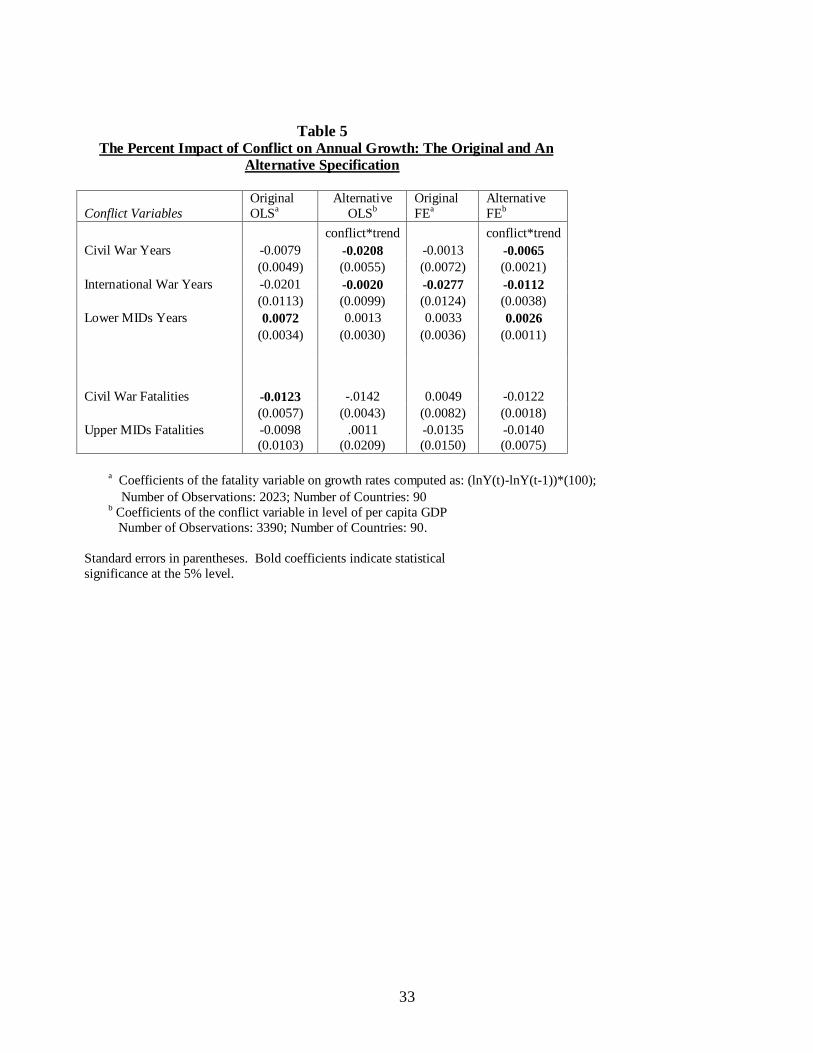
VII.F Robustness Checks

We also check the sensitivity of our results to changes in model specification. To

do so, we re-specify the dependent variable to be income level expressed as a logarithm

of real GDP per capita (as opposed to the change in the logarithm of per capita GDP). In

addition to the previous explanatory variables, we include a trend variable, a conflict

variable27

and a trend-conflict interaction term. More formally, the specification is:

ititititit tZZty 3210ln (6)

where Z denotes the conflict variable and t the time trend. The interaction term

coefficient indicates the change in growth due to conflict. it is the vector of control

variables, which include trade, central government budget balance, institutional quality

index, rate of population growth, life expectancy, investment, and government

consumption. If the coefficient on the interaction variable is similar to the coefficient on

the conflict variable in the original specification (where conflict duration and intensity

measures are used), then both models are compatible, indicating similar implications

regarding the effect of conflict on growth. The results are shown in Table 5. Here civil

wars are related to a decrease in growth by 2% (OLS) and 0.6% (FE). As before the

higher OLS coefficient implies less quickly growing countries are more prone to civil

war. International wars are related to an annual decrease of .2 (OLS) to 1.2 (FE) percent

in the level of GDP, while low-intensity conflict raises income from .13 (OLS) to .26

27

We run five separate regressions, one for each conflict variable. The first three (civil war, international

war and lower MID) are dichotomous variables which equal one if participating in a war and zero if not.

The latter two measure war severity (the number of battle deaths in civil or international wars).

20

(FE) annually. Here FE magnitudes exceed OLS estimates indicating a decline in growth

even accounting for heterogeneity. Again, we find (especially for the FE estimation) that

war casualties provide a strong measure of the negative effects of conflict on GDP level.

Overall, we corroborate that both civil and international wars are associated with reduced

growth, while low-intensity conflict may enhance it.

An important question about these results is robustness across countries. Do all

countries exhibit the same effects of war? We answer this question in the next section.

VIII. Sub-Sample Analysis

To answer the above question regarding robustness across countries, we rerun

equation (5) in three ways. First we break the countries up into five specific regions;

second we examine countries based on polity; and third we separate counties by income

level. Again we use both five-year and annual time intervals. As before, we find that

sociopolitical conflict reduces growth, but the degree conflict lessens growth varies

across country wealth, polity and conflict severity.28

VIII.A Regional Differences

The regional sub-samples we use are: 25 OECD countries, 22 Latin America, 29

Africa, and six Asian Tigers, each identified in Appendix A. Table 6 (Panel A) contains a

summary of the analysis. We present coefficients for the three variables indicating the

number of years at war (civil war years, international war years, and lower MIDs years)

as well as for the civil and international war fatalities variables. We find civil wars

negatively related to growth in most countries, and interstate wars especially detrimental

to African country growth rates.

28

As a robustness check, we also test a model specification where we interact years at war, and then war

fatality variables with regional, income, and polity dichotomous variables (each dummy is also added

separately, and the constant is suppressed in OLS estimation). Whether one- or five-year time intervals are

analyzed, the results are quantitatively and qualitatively comparable.

21

More specifically, in the OECD sample (column 1), only fatalities yield

statistically significant results. Here a one-unit increase in civil war fatalities is associated

with a decrease in growth by 60%. To put this in perspective, this means that an OECD

country experiences a 60% decline in growth if one-thousandth of its population dies in a

civil war. It experiences a 164% decline if one-thousandth of its population dies in an

international war.

For Latin America (column 2), no statistically significant effects were

discernable. However, African countries exhibited large effects when wars are measured

by fatalities (column 3).29

A civil war mortality of one-thousandth population decreases

growth by over 4% and an international mortality rate of one-thousandth of population

decreases growth by 284%. The analysis of the Asian Tigers sample (column 4) shows

negative (though statistically insignificant) growth rate effects for both civil war and

international war fatalities. We found no statistically significant results for OPEC nations,

except with regard to international wars, which in several model specifications appear to

increase the rate of economic growth in oil exporting countries. One explanation of the

positive effect of conflict on growth in the OPEC member nations might be OPEC oil

producers suffer no gains from trade losses arising from conflict given the highly

strategic nature of oil.

A possible explanation as to why there is so much variation in the impact of civil

war fatalities on economic growth by country and by region might be that certain dyads

experience multiple types of sociopolitical violence which arise due to complex causes

and either overlap or closely follow in time, thereby reducing the prospect of economic

recovery. This protracted and severe conflict would then have a particularly strong

growth-reducing effect, as we have seen in the magnitudes of the estimated coefficients.

29

These results are not driven by too few instances of war. Interstate wars in Africa include Uganda-Sudan,

Chad-Sudan, Congo (former Zaire) and six other involved states, Ethiopia-Eritrea, and Tanzania-Uganda.

And, according to Miguel, Satyanath, Sergenti (2003) “The major locus for civil wars in recent years has

been Sub-Saharan Africa, where twenty seven of forty countries suffered from civil conflict during the

1980s and 1990s (PRIO 2002).”

22

Below are some examples of such complex conflicts where countries were

simultaneously involved in inter- and intra-state hostilities, respectively.

(1) Vietnam-Cambodia War 1975-1979 and Cambodia vs. Khmer Rouge 1970-

1975.

(2) Bangladesh War 1971 and Pakistan vs. Bengalis 1971.

(3) Ethiopia-Somalia War 1977-1978 and Ethiopia vs. Somali Rebels 1976-1977,

Ethiopia vs. Tigrean Liberation Front 1978-1991, Ethiopia vs. Eritrean Rebels

1974-1991.

(4) Uganda-Tanzania War 1978-1979 and Uganda vs. National Resistance Army

1980-1988.

(5) Iran-Iraq War 1980-1988 and Iran vs. Mujaheddin 1981-1982.

VIII.B Differences by Income Groups

Next, we posit that the effects of conflict vary from rich to poor economies. Using

income level categories defined by the World Bank, we divide all the countries into three

sub-samples based on income level. In line with the official classification, economies are

divided into three groups according to 2005 GNI per capita: low income, $875 or

less; lower middle income, $876 - $3,465; upper middle income, $3,466 - $10,725;

and high income, $10,726 or more.30

For simplicity, the two middle income categories

were combined into a single middle income category, thus yielding three sub-samples for

this study, i.e. high income, middle income, and low income countries. Each group of

countries was estimated individually. The results are contained in Table 6 (Panel B).

30

http://web.worldbank.org/

23

The analysis for the 25 high-income countries (column 1) reveal that deaths from

international wars reduce the income growth rate (fatality measures are statistically

significant for both the five-period and one-year analyses). No significant relationships

were found in the middle-income grouping of 39 countries (column 2). Lastly, the

examination of 16 low-income countries reveals the negative influences of fatalities from

international war on economic growth (column 3). This result is consistent with that

found in the African regional sample, and supports the contention that poor economies

suffer the largest income growth reduction from the damage inflicted by war.

VIII.C Differences by Political Regime

It is also plausible that whether a given country is democratic or non-democratic

determines how it would be affected by various forms of conflict. To explore this venue,

the total sample was divided into two sub-samples using the democracy criterion.

For this purpose, we utilized the polity variable from Polity IV data. This measure

assigns each country a democracy score ranging from „-10‟ to „10‟, including a „0‟. Based

on this variable, countries with a score of „6‟ or above were considered democratic, and

those with a score below „6‟ were treated as non-democratic (Panel C).

In the sample of 56 democratic countries, there is a positive relationship between

non-fatal conflict, or lower-level MIDs and economic growth rate. This finding reinforces

the same result obtained for the OECD and high-income sub-samples, along with the

hypothesis that containment of conflict at the lower level of hostility is conducive to

economic growth.

Secondly, for democratic countries fatalities from international wars are

associated with decreased growth – a finding not unlike that for high-income countries,

and just as robust to changes in model specification. In 35 non-democratic countries,

fatalities from civil wars are found to be negatively related to growth and statistically

significant.

24

The results for our regional analyses were also tested using the alternative

specification described at the end of the previous section. The testing confirmed that

Asian Tigers, African, and poor countries experience large negative effects of wars, while

high-income countries and democracies, mostly face growth-reducing effects from

international wars.

IX. Conclusion

This study examines economic consequences of war within the empirical growth

framework. To do so, we utilize panel data for 90 countries spanning 1970-2000. The

data include real per capita GDP, country specific attributes, as well as five measures of

domestic and international wars. From these we concentrate on how civil and

international wars relate to country growth. We use short-term annual time-periods to get

at the immediate effects of war, as well as time-periods spanning two, five and thirty

years to get at long-term effects.

Our statistical analyses comprise both ordinary least squares and fixed-effects

estimation techniques. The latter FE techniques hold constant country specific effects

enabling us to measure the effects of wars within countries. The former amalgamate both

cross-country and country-specific effects. Comparing results from both approaches

enables us to make inferences about causality, namely whether more quickly growing

countries are more likely to initiate conflict. Further, we stratify by our sample, re-

performing the analysis by region, country wealth, and polity to examine whether the

effects of war differ by country type.

Our main conclusions are: (1) The short-term effects of conflict are more

pronounced than long-term effects. In short, countries recover from wars. (2) Poorer low-

growth countries appear prone to civil wars, whereas richer high-growth countries to

interstate wars. The effect of both is to decrease economic growth. Civil wars negatively

affect all countries, and especially affect non-democracies. Interstate wars appear

especially detrimental to African countries. (3) War severity measured by fatalities as a

percent of a country‟s population appears to yield more robust measures of the effect of

25

wars on country growth than war duration. Finally, (4) low-income countries suffer from

wars more than high-income countries.

26

Figure 1: Conflict and Per Capita GDP

6.8

77

.27

.47

.6

1970 1980 1990 2000year

IntWar No Force

DomWar Int/Dom

Int/NoF NoF/Dom

Int/NoF/Dom (log) GDP

Conflict - UGA

8.8

8.9

99

.19

.29

.3

1970 1980 1990 2000year

IntWar No Force

DomWar Int/Dom

Int/NoF NoF/Dom

Int/NoF/Dom (log) GDP

Conflict - TUR

6.9

77

.17

.27

.37

.4

1970 1980 1990 2000year

IntWar No Force

DomWar Int/Dom

Int/NoF NoF/Dom

Int/NoF/Dom (log) GDP

Conflict - BDI

8.7

8.8

8.9

99

.1

1970 1980 1990 2000year

IntWar No Force

DomWar Int/Dom

Int/NoF NoF/Dom

Int/NoF/Dom (log) GDP

Conflict - COL

8.8

8.9

99

.19

.29

.3

1970 1980 1990 2000year

IntWar No Force

DomWar Int/Dom

Int/NoF NoF/Dom

Int/NoF/Dom (log) GDP

Conflict - DZA

6.8

6.9

77

.17

.2

1970 1980 1990 2000year

IntWar No Force

DomWar Int/Dom

Int/NoF NoF/Dom

Int/NoF/Dom (log) GDP

Conflict - ETH

7.4

7.6

7.8

88

.28

.4

1970 1980 1990 2000year

IntWar No Force

DomWar Int/Dom

Int/NoF NoF/Dom

Int/NoF/Dom (log) GDP

Conflict - IND

7.8

88

.28

.48

.6

1970 1980 1990 2000year

IntWar No Force

DomWar Int/Dom

Int/NoF NoF/Dom

Int/NoF/Dom (log) GDP

Conflict - LKA

27

88

.59

1970 1980 1990 2000year

IntWar No Force

DomWar Int/Dom

Int/NoF NoF/Dom

Int/NoF/Dom (log) GDP

Conflict - NIC

9.6

9.8

10

10

.2

1970 1980 1990 2000year

IntWar No Force

DomWar Int/Dom

Int/NoF NoF/Dom

Int/NoF/Dom (log) GDP

Conflict - ISR

7.4

7.6

7.8

88

.2

1970 1980 1990 2000year

IntWar No Force

DomWar Int/Dom

Int/NoF NoF/Dom

Int/NoF/Dom (log) GDP

Conflict - PAK

8.7

8.8

8.9

99

.19

.2

1970 1980 1990 2000year

IntWar No Force

DomWar Int/Dom

Int/NoF NoF/Dom

Int/NoF/Dom (log) GDP

Conflict - PER

6.8

77

.27

.47

.67

.8

1970 1980 1990 2000year

IntWar No Force

DomWar Int/Dom

Int/NoF NoF/Dom

Int/NoF/Dom (log) GDP

Conflict - RWA

8.8

8.9

99

.19

.2

1970 1980 1990 2000year

IntWar No Force

DomWar Int/Dom

Int/NoF NoF/Dom

Int/NoF/Dom (log) GDP

Conflict - SLV

7.4

7.6

7.8

88

.2

1970 1980 1990 2000year

IntWar No Force

DomWar Int/Dom

Int/NoF NoF/Dom

Int/NoF/Dom (log) GDP

Conflict - TCD

77

.58

8.5

1970 1980 1990 2000year

IntWar No Force

DomWar Int/Dom

Int/NoF NoF/Dom

Int/NoF/Dom (log) GDP

Conflict - CHN

28

Table 1

Summary Statistics for All Variables

Abbreviation

Definitiona Mean Std. Dev. Min Max

Grlngdp The average growth rate of real GDP

per economically active population in

1970-2000 (PWT6.1).

1.256861 2.012491 -3.23467 7.246649

Laglngdp The log of real GDP per economically

active population in the base period

(PWT6.1).

8.594688 .9428799 6.619124 10.41

Open The trade openness index [0,1] as the share of years a country was integrated

into the global economy in 1970- 2000

(based on Sachs and Warner 1995,

1997).

.3469019 .4358744 0 1

Open*Laglngdp Interaction of “open” and “laglngdp”,

1970-2000.

3.206776 4.137016 0 10.41

Tropics The share of country subjected to a tropical climate [0,1] (Sachs and

Warner 1997).

.5677686 .4701445 0 1

Access Landlocked country dummy, i.e. no

access to sea = (Sachs and Warner

1995, 1997).

.1885246 .3927434 0 1

Cgb Central government budget balance,

computed as central government revenues minus expenditures as a share

of GDP, i.e. average government

savings in 1970-2000 (WDI2004).

-3.169499 5.653045 -23.51052 18.2243

Icrgeb Institutional quality index (10- point

scale) in 1970-2000 published by the

PRS group (IRIS-3).

5.653712 2.203877 2.185714 9.988571

Grpop Growth rate of economically active population minus the growth rate of

total population in 1970-2000

(WDI2004).

.2572844 .4089627 -.7131408 1.256329

Sxp Share of primary product exports (fuel

and non-fuel) in real GDP in the base

period (WDI2004).

.1198699 .163954 .0024843 .89

Exlife Average life expectancy in the base period (WDI2004).

56.24249 11.72529 34.36341 74.64927

Exlifesqr The square of “exlife”. 3299.554 1322.642 1180.844 5572.513

Polity2 Democracy measure from Polity IV project, variable polity2.

.6910638 7.552719 -10 10

Trade Share of imports and exports in real

GDP in 1970-2000 (WDI2004).

68.92663 42.07816 7.979733 274.1847

a The data sources are abbreviated as follows: Penn World Tables Mark6.1 – PWT6.1; World Development

Indicators 2004, World Bank – WDI2004; IRIS-3 – International Risk Investment Survey, International Country Risk Guide (ICRG) Data by the Political Risk Services group; COW – Correlates of War,

available online from Pennsylvania State University; MID – Militarized Interstate Dispute data compiled

by the COW project. b See text for a more detailed description of the index.

29

Table 1, Continued

Investment Share of gross fixed capital formation in

real GDP in 1970-2000 (WDI2004).

21.21366 6.841431 2.23354 58.57447

Ggc Share of the general government final consumption expenditures in real GDP

in 1970-2000 (WDI2004).

15.92191 6.623317 3.135428 56.40001

Sumdomwarc Number of years engaged in civil war in

1970-2000 (COW v3.0) years.

.0858704 .1936608 0 .9047619

Summidnofatal Aggregated interstate events data on:

lower MIDs 1-3, no militarized action,

threat to use, and display of force; number of years engaged in low-level

MIDs in 1970-2000 (MID v3.02 data).

.1807182 .1827372 0 .9047619

Summidfatal Aggregated interstate events data on:

upper MIDs 4-5, use of force and war;

number of years engaged in upper-level

MIDs in 1970-2000 (MID v3.02 data).

.204918 .2419514 0 .9047619

Summidward Number of years engaged in international war in 1970-2000 (MID

v3.02 data).

.0249805 .0770059 0 .5238096

Civfatality Number of deaths from civil war per

thousand of population in 1970-2000

(COW v3.0).

.6805628 4.081746 0 70.13132

Midfatality Number of deaths from fatal forms of

conflict per thousand of population, i.e.

upper MIDs (use of force and war) in 1970-2000 (MID v3.02).

.1019104 .9885795 0 14.63357

c Each war and conflict variable is coded as a dummy in models based on annual data.

d The correlation coefficient (significant at the .05 level) between interstate war index computed with COW

data and the index computed with MIDs data is 0.9122, i.e. the two datasets do not exactly map into each

other. The data used are from COW V3.0, Inter-state War Participants (data on state participation in inter-

stat wars) and midB V3.02 (data on MIDs from 1816-2001, at the participant level; contains one record per

militarized dispute participant.)

30

Table 2

Conflict Variables: Correlation Coefficients31

Five-Year Time

Intervals

Civil War Years 1

International War Years 0.0322 1

Lower MIDs Years -0.2727 0.114 1

Two-Year Time

Intervals

Civil War Years 1

International War Years -0.064 1

Lower MIDs Years -0.5885 -0.2399 1

One-Year Time

Intervals

Civil War Years 1

International War Years -0.0728 1

Lower MIDs Years -0.9236 -0.2082 1

31

Missing observations for these variables were deleted for the purpose of estimating the correlation

coefficients.

31

Table 3 Single Cross-Section OLS Results, 1970-2000

Independent Variables Variations*

Sachs-Warner (1) (2) (3)

lagged income -1.5084 -1.2660 -1.2625 -1.2747

(Laglngdp) (0.2305) (0.2553) (.2512) (.2582)

openness index 10.7347 9.9590 9.3253 9.8867

(Open) (2.9312) (4.3502) (4.5060) (4.4173)

openness index*lagged income -1.0512 -.9906 -.9022 -.9840

(Open*Laglngdp) (0.3577) (0.5113) (.5322) (.5194)

Tropics -0.8532 -1.3244 -1.1865 -1.3853

(Tropics) (0.2787) (0.3354) (.3653) (.3638)

landlocked -0.5904 -.0702 -.1144 -.0862

(Access) (0.2504) (0.3447) (.3575) (.3511)

government budget balance .1165

(Cgb) (.0220)

institutional quality index .3070 .4025 .3807 .3918

(Icrge) (.0819) (.1408) (.1466) (.1442)

population growth .7716 .0320 .0645 -.0186

(Grpop) (.3648) (.5271) (.5404) (.5491)

primary product exports -3.9538

(Sxp) (.9850)

life expectancy .3338 .1944 .2091 .2104

(Exlife) (.1224) (.1715) (.1820) (.1771)

life expectancy squared -.0025 -.0012 -.0014 -.0014

(Exlifesqr) (.0011) (0.0016) (.0017) (.0016)

civil war -.4975

(Sumdomwar) (.6918)

international war 2.0926

(Summidwar) (2.4625)

lower MIDs -.0166

(Summidnofatal) (.7419)

civil war fatality -9.21e-07

(Civfatality) (1.95e-06)

upper MIDs fatality -3.05e-07

(Midfatality) (1.43e-06)

Constant 2.0584 2.9919 2.6058 2.7834

(3.3211) (4.9272) (5.0711) (5.0055)

R-squared 0.8666 0.6223 .6294 .6237

Dependent variable is average growth rate of real GDP per worker in 1970-2000

(log difference in real GDP per working age person divided by the number of years)

White's robust standard errors are in parentheses. Number of observations = 81.

Bold coefficients indicate statistical significance at the 5% level.

32

Table 4

The Percent Impact of Conflict on Growth Between (OLS) and Within (Fixed-Effects)

Countries

Five-Year Time Intervals

Conflict Variables Fixed-Effects OLS Fixed-Effects OLS

Civil War Years -.0118 -0.1076 -0.1008 -0.4689

(0.1150) (0.0898) (0.5298) (0.3979)

International War

Years -0.1782 .3024 -0.5493 0.9907

(.2175) (.2027) (1.0270) (0.9479)

Lower MIDs Years 0.1551 0.1414 0.6483 0.4800

(0.1095) (0.0851) (0.5380) (0.4090)

Civil War Fatalities -.2145 -.2568 -0.2698 -0.2515

(0.1252) (0.1062) (0.1220) (0.1028)

Upper MIDs Fatalities -.4778 -0.1816 -0.3941 -0.1333

(.2549) (.2043) (0.2520) (0.1986)

Two-Year Time Intervals

Fixed-Effects OLS Fixed-Effects OLS

Civil War Years 0.0178 -0.2458 -0.0450 -0.1318

(.1859) (0.1408) (0.1494) (0.1133)

International War

Years -0.6683 -0.1060 -0.4992 -0.1289

(.3424) (0.3180) (0.2725) (0.2540)

Lower MIDs Years 0.0610 0.2019 .1260 0.1831

(.1236) (0.1088) (0.0992) (0.0875)

Civil War Fatalities 0.3284 -0.6607 -0.0497 -0.7131

(0.5633) (0.3496) (0.4553) (0.2806)

Upper MIDs Fatalities -2.5783 -0.4233 -2.2010 -1.0595

(1.0607) (0.7092) (0.8529) (0.5689)

One-Year Time Intervals

Fixed-Effects OLS Fixed-Effects OLS

Civil War Years -0.1286 -0.7921 -0.2446 -0.4931

(0.7211) (0.4940) (0.4295) (0.3226)

International War

Years -2.7735 -2.0070 -1.4438 -0.6605

(1.2442) (1.1328) (0.7146) (0.6967)

Lower MIDs Years 0.3256 0.7246 -0.0610 0.3161

(0.3619) (0.3351) (0.2365) (0.2242)

Civil War Fatalities 0.4867 -1.2303 0.1664 -1.1008

(0.8168) (0.5685) (0.6118) (0.4336)

Upper MIDs Fatalities -1.3527 -0.9761 -2.2506 -1.4936

(1.5043) (1.0347) (1.1209) (0.7888)

Coefficients of growth regressions where dependent variables is the average growth rate of real GDP per worker

over each specified time-period (log difference in real GDP per working age person divided by the number of year

in the time period) and the independent variables are the indicated conflict measures. The left two columns repeat results reported in Tables 3 and 4. The right two columns use two-year moving average data for growth.

Standard errors in parentheses.

33

Table 5

The Percent Impact of Conflict on Annual Growth: The Original and An

Alternative Specification

Conflict Variables

Original

OLSa

Alternative

OLSb

Original

FEa

Alternative

FEb

conflict*trend conflict*trend

Civil War Years -0.0079 -0.0208 -0.0013 -0.0065

(0.0049) (0.0055) (0.0072) (0.0021)

International War Years -0.0201 -0.0020 -0.0277 -0.0112

(0.0113) (0.0099) (0.0124) (0.0038)

Lower MIDs Years 0.0072 0.0013 0.0033 0.0026

(0.0034) (0.0030) (0.0036) (0.0011)

Civil War Fatalities -0.0123 -.0142 0.0049 -0.0122

(0.0057) (0.0043) (0.0082) (0.0018)

Upper MIDs Fatalities -0.0098 .0011 -0.0135 -0.0140

(0.0103) (0.0209) (0.0150) (0.0075)

a Coefficients of the fatality variable on growth rates computed as: (lnY(t)-lnY(t-1))*(100);

Number of Observations: 2023; Number of Countries: 90 b Coefficients of the conflict variable in level of per capita GDP

Number of Observations: 3390; Number of Countries: 90.

Standard errors in parentheses. Bold coefficients indicate statistical

significance at the 5% level.

34

Table 6

The Percent Impact of conflict on Growth

Fixed Effects Results, 1970-2000 by Country Type

(A) The Impact of Conflict on Growth by Type of Country Based on Region

Five-Year time Intervals

Conflict Variables OECD Latin America Africa Asian Tigers OPEC

Civil War Years -0.3215 -0.1065 -0.6000 -6.3720 -4.0970

(1.4585) (1.3125) (1.0475) (3.4510) (2.8910)

International War Years 2.2440 -3.8870 7.5445

(2.2990) (1.9870) (2.3225)

Lower MIDs Years 0.6830 -0.1090 -0.6895 1.2970 -2.7680

(0.6215) (1.6120) (1.0570) (1.5985) (2.1430)

Civil War Fatalities -17.5750 -0.3025 -2.6745 -516.1620 -12.9435

(26.7300) (1.0385) (1.7765) (283.1155) (11.3590)

Upper MIDs Fatalities 3.6600 -91.7735 -186.6205 -383.7675 -0.5290

(54.3205) (124.4770) (49.4200) (1363.3195) (2.7675)

Growth rates computed as: (lnY(t)-lnY(t-5))*(100/5); adjusting for lagged income, trade share,

government budget balance, institutional quality index, population growth, life expectancy, investment

share, and government consumption share. Standard errors in parentheses.

One-Year Time Intervals

Conflict Variables

OECD Latin America Africa Asian Tigers OPEC

Civil War Years -1.0256 -0.8871 0.0597 1.9587

(2.1741) (1.2960) (1.6492) (2.6717)

International War Years -2.1049 -9.5642 2.0282

(1.1585) (3.5987) (3.9043)

Lower MIDs Years 0.1694 -0.3083 -0.6364 0.0099 2.7167

(0.3481) (0.8365) (0.8681) (0.5900) (1.9857)

Civil War Fatalities -60.2666 1.9495 -4.0767 -593.7900 60.4447

(27.4388) (1.1982) (2.5492) (424.3470) (46.3470)

Upper MIDs Fatalities -164.2300 -0.9357 -284.1224 -962.6589 4.9457

(109.2633) (116.0157) (83.5672) (1464.6840) (3.0316)

Growth rates computed as: (lnY(t)-lnY(t-1))*(100); adjusting for lagged income, trade share, government

budget balance, institutional quality index, population growth, life expectancy, investment share, and

government consumption share. Standard errors in parentheses.

35

(B) The Impact of Conflict on Growth by Type of Country Based on Income

Five-Year time Intervals

Growth rates computed as: (lnY(t)-lnY(t-5))*(100/5); adjusting for lagged income, trade share, government

budget balance, institutional quality index, population growth, life expectancy, investment share, and

government consumption share. Standard errors in parentheses.

One-Year Time Intervals

Conflict Variables High-Income Middle-Income Low-Income

Civil War Years -0.0546 -0.3758

(1.1004) (1.2557)

International War Years -1.9325 -0.3804 -18.0264

(1.1006) (2.0616) (4.1693)

Lower MIDs Years 0.1515 0.6736 -0.8033

(0.3679) (0.6068) (0.8678)

Civil War Fatalities 2.2254 -1.2089

(1.0412) (2.1999)

Upper MIDs Fatalities -58.3862 -1.7831 -311.6659

(11.1185) (1.6623) (100.9576)

Growth rates computed as: (lnY(t)-lnY(t-1))*(100); adjusting for lagged income, trade share, government

budget balance, institutional quality index, population growth, life expectancy, investment share, and

government consumption share. Standard errors in parentheses. Bold coefficients indicate statistical

significance at the 5% level.

Conflict Variables High-Income Middle-Income Low-Income

Civil War Years -0.1420 0.3055

(0.8390) (1.3590)

International War Years -1.028 0.3295 -5.6685

(1.4605) (1.8070) (3.5240)

Lower MIDs Years 1.1755 -0.0165 -0.1300

(0.7350) (0.9205) (1.3175)

Civil War Fatalities -0.1210 -0.3875

(0.8525) (1.2410)

Upper MIDs Fatalities -22.4225 -2.0675 -220.0240

(6.7875) (1.4465) (76.9985)

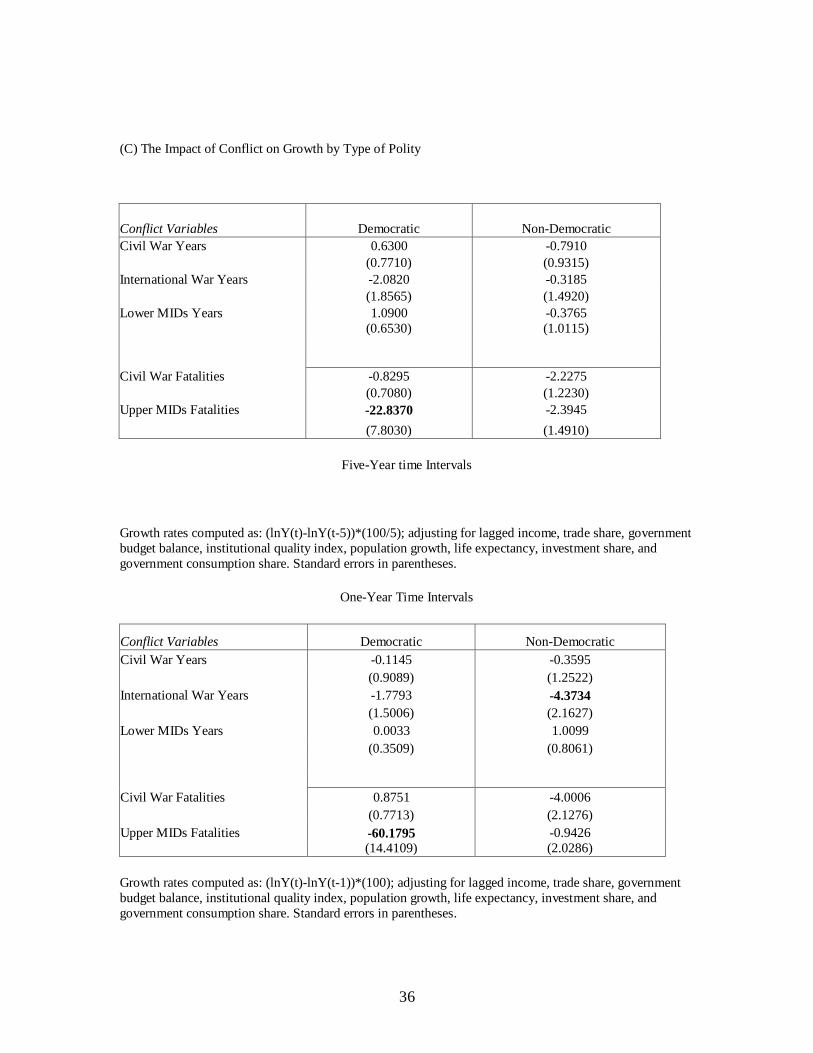
36

(C) The Impact of Conflict on Growth by Type of Polity

Five-Year time Intervals

Growth rates computed as: (lnY(t)-lnY(t-5))*(100/5); adjusting for lagged income, trade share, government

budget balance, institutional quality index, population growth, life expectancy, investment share, and

government consumption share. Standard errors in parentheses.

One-Year Time Intervals

Conflict Variables Democratic Non-Democratic

Civil War Years -0.1145 -0.3595

(0.9089) (1.2522)

International War Years -1.7793 -4.3734

(1.5006) (2.1627)

Lower MIDs Years 0.0033 1.0099

(0.3509) (0.8061)

Civil War Fatalities 0.8751 -4.0006

(0.7713) (2.1276)

Upper MIDs Fatalities -60.1795 -0.9426

(14.4109) (2.0286)

Growth rates computed as: (lnY(t)-lnY(t-1))*(100); adjusting for lagged income, trade share, government

budget balance, institutional quality index, population growth, life expectancy, investment share, and

government consumption share. Standard errors in parentheses.

Conflict Variables Democratic Non-Democratic

Civil War Years 0.6300 -0.7910

(0.7710) (0.9315)

International War Years -2.0820 -0.3185

(1.8565) (1.4920)

Lower MIDs Years 1.0900 -0.3765

(0.6530) (1.0115)

Civil War Fatalities -0.8295 -2.2275

(0.7080) (1.2230)

Upper MIDs Fatalities -22.8370 -2.3945

(7.8030) (1.4910)

37

References

Aizenman, Joshua, and Nancy Marion. 1993. “Macroeconomic Uncertainty and Private

Investment.” Economic Letters 41: 207-210.

Alesina, A., Easterly, W., and Matuszeski, J. 2006. “Artificial States.” NBER Working

Paper No. 12328.

Alesina, A., Devleeschauwer, A., Easterly, W., Kurlat, S., Wacziarg, R. 2003.

“Fractionalization.” Journal of Economic Growth 8(2): 155-194.

Alesina, Alberto F., Sule Oezler, Nouriel Roubini, and Philip Swagel. 1996. “Political

Instability and Economic Growth.” Journal of Economic Growth 1: 189-211.

Alesina, Alberto F., and Roberto Perotti. 1996. “Income Distribution, Political Instability

and Investment.” European Economic Review 80: 1203-1228.

Alesina, Alberto F., and Guido Tabellini. 1989. “External Debt, Capital Flight and

Political Risk.” Journal of International Economics 27:199-220.

Barro, Robert J. 1991. “Economic Growth in a Cross Section of Countries,“Quarterly

Journal of Economics 106(2): 407-444.

Barro, Robert J. 1997. Determinants of Economic Growth: A Cross-Country Empirical

Study. Lionel Robbins Lectures. Cambridge, Mass.: MIT Press.

Barro, Robert J., and Jong-Wha Lee. 1993. “Losers and Winners in Economic Growth.”

NBER Working Paper No. 4341.

Barro, Robert J., and Xavier Sala-i-Martin. 1992. “Convergence.” The Journal of

Political Economy 100(2): 223-251.

38

Barro, Robert J., and Xavier Sala-i-Martin. 1995. “Economic Growth.” New York:

McGraw-Hill.

Barro, Robert J., and Holger Wolf. 1989. “Data Appendix for Economic Growth in a

Cross Section of Countries.” Mimeo Cambridge MA.: Harvard University.

Baumol, William J. 1986. “Productivity Growth, Convergence, and Welfare: What The

Long-Run Data Show?” American Economic Review LXXVI (1986): 1072-1085.

Beck, Nathaniel, and Jonathan N. Katz. 1995. “What to Do (and Not to Do) with Time-

Series Cross-Section Data.” The American Political Science Review 89(3): 634-647.

Blomberg, S. Brock, and Gregory D. Hess. 2002. “The Temporal Links between Conflict

and Economic Activity.” The Journal of Conflict Resolution 46(1): 74-90.

Borooah, V.K., and Paldam, M. 2007. “Why is the world short of democracy?: Across-

country analysis of barriers to representative government.” European Journal of Political

Economy 23: 582-604.

Brock, W., and Durlauf, S. 2002. “Market Implications of Peer and Neighborhood

Effects: A Multinomial Choice Model of Neighborhood Effects.” American Economic

Review 92(2): 298-303.

Brunetti, Aymo. 1997. “Political Variables in Cross-Country Growth Analysis,” Journal

of Economic Surveys 11: 163-190.

Burnside, Craig, and David Dollar. 2000. “Aid, Policies, and Growth.” American

Economic Review 90(4): 847-868.

Butkiewicz, James L., and Halit Yanikkaya. 2005. “The Impact of Sociopolitical

Instability on Economic Growth: Analysis and Implications,” Journal of Policy

Modeling, 27: 629-645.

39

Chauvet, Lisa. 2003. "Socio-political instability and the allocation of international aid by

donors," European Journal of Political Economy, Elsevier, 19(1): 33-59.

Collier, Paul. 2007. The Bottom Billion: Why the Poorest Countries Are Failing and

What Can Be Done About It. Oxford University Press.

Collier, Paul, Lance Elliot, Håvard Hegre, Anke Hoeffler, Marta Reynal-Querol, and

Nicholas Sambanis. 2003. Breaking the Conflict Trap: Civil War and Development

Policy. Oxford and Washington DC: Oxford University Press and World Bank.

Collier, Paul, and Nicholas Sambanis. 2002. “Understanding Civil War: A New Agenda.”

Journal of Conflict Resolution 46(1): 3-12.

Diehl, Paul F. 1983. “Arms Races and Escalation: A Closer Look.” Journal of Peace

Research 20(3): 205-212.

Dixit, Avinash K., and Robert S. Pindyck. 1994. “Investment Under Uncertainty.”

Princeton: Princeton University Press: 14-468.

Dollar, David, and Jakob Svensson. 2000. “What Explains the Success of Failure of

Structural Adjustment Programmers.” Economic Journal 110: 894-917.

Doucouliagos, H. and M. Paldam. 2008. “Aid effectiveness on growth: A meta-study.”

European Journal of Political Economy 24: 1 - 24.

Forbes, Kristin J. 2000. “A Reassessment of the Relationship between Inequality and

Growth.” American Economic Review 90: 869-887.

Easterly, William, Michael Kremer, Lant Pritchett, and Laurence Summers. 1993. “Good

Policy or Good Luck? Country Performance and Temporary Shocks.” Journal of

Monetary Economics 32: 459-483.

40

Easterly, William, and Ross Levine. 1997. “Africa‟s Growth Tragedy: Policies and

Ethnic Divisions.” Quarterly Journal of Economics 112: 1203-1250.

Easterly, William, and Sergio Rebelo. 1993. “Fiscal Policy and Economic Growth: An

Empirical Investigation.” Journal of Monetary Economics 32: 417-458.

Hall, R., and Jones, C. 1999. “Why Do Some Countries Produce So Much More Output

Per Worker Than Others?” The Quarterly Journal of Economics, MIT Press 114(1): 83

116.

Hall, Robert E., and Charles I. Jones. 1997. “Levels of Economic Activity Across

Countries,” American Economic Review, American Economic Association 87 (2): 173-

77.

Hillman, A. L. 2009. Public Finance and Public Policy: Responsibilities and Limitations

of Government (2nd Ed.). Cambridge University Press, New York.

Hillman, A.L., and Konrad, K.A. 2008. Forty Years of Research on Rent Seeking, Volume

II, Applications: Rent Seeking in Practice. Springer, Berlin: 245-264.

Hillman, A.L. 2004. “Nietzschean development failures.” Public Choice 119: 263-280.

Islam, Nazrul. 1995. “Growth Empirics: A Panel Data Approach.” The Quarterly Journal

of Economics 110(4): 1127-1170.

Jong-A-Pin, R. 2009. “On the measurement of political instability andits impact on

economic growth.” European Journal of Political Economy 25: 15-29.

Knack, Stephen, and Philip Keefer. 1995. “Institutions and Economic Performance:

Cross-Country Tests Using Alternative Institutional Measures.” Economics and Politics

7: 207-227.

41

Landau, Daniel. 1986. “Government and Economic Growth in the LDCs: An Empirical

Study for 1960-1980.” Economic Development and Cultural Change 35: 35-76.

Levine, Ross, and David Renelt. 1992. “A Sensitivity Analysis of Cross-Country Growth

Regressions.” American Economic Review 82: 942-963.

Londregan, John B., and Keith Poole. 1990. “Poverty, the Coup Trap, and the Seizure of

Executive Power.” World Politics 42: 151-183.

Mankiw, N. Gregory, David Romer, D., and David N. Weil. 1992. “A Contribution to the

Empirics of Economic Growth.” Quarterly Journal of Economics 107 (2): 407-438.

Mauro, P. 1995. “Corruption and Growth.” Quarterly Journal of Economics 110: 681-

712.

McCleary, Rachel M., and Barro, Robert J. 2006. “Religion and Economy.” Journal of

Economic Perspectives 20 (2): 49-72.

Mehlum, H., Moene, K., and Torvik, R. 2006. “Institutions and the resource curse.”

Economic Journal 116: 1-20. Reprinted in: Congleton, R.D.,

Merrouche, O. 2008. “Landmines and Poverty: IV Evidence from Mozambique.”

Peace Economics, Peace Science and Public Policy 14, issue 1, article 2,

http://www.bepress.com/peps/vol14/iss1/2.

Miguel, Edward, Shanker Satyanath, and Ernest Sergenti. 2003. “Economic Shocks and

Civil Conflict: An Instrumental Variables Approach,” Working Paper available at

http://web.mit.edu/14.773/www/conflict_15apr03.pdf.

Montalvo, J., and Reynal-Querol, M. 2005. “Ethnic Polarization, Potential Conflict, and

Civil Wars.” American Economic Review 95(3): 796-816.

Murdoch, James C., and Todd Sandler. 2002. “Economic Growth, Civil Wars, and

Spatial Spillovers.” Journal of Conflict Resolution 46(1): 91-110.

42

Murdoch, James C., and Todd Sandler. 2004. “Civil Wars and Economic Growth: Spatial

Dispersion.” American Journal Political Science 48(1): 138-151.

North, D. 1990. “Institutions, Institutional Change and Economic Performance.”

Cambridge University Press.

Parente, Stephen L., and Edward C. Prescott. 1994. “Barriers to Technology Adoption

and Development.” Journal of Political Economy 102 (2): 298-321.

Persson, Torsten., and Lars E. Svensson. 1989. “Why a Stubborn Conservative Would

Run a Deficit: Policy with Time Inconsistent Preferences.” Quarterly Journal of

Economics 104: 325-245.

Persson, Torsten, and Guido Tabellini. 2006. “Democracy and Development: the Devil in

the Details.” CESIFO Working Paper No.1672.

Polachek, Solomon W. 1980. “Conflict and Trade.” The Journal of Conflict Resolution

24 (1): 55-78.

Polachek, Solomon W. 1997. “Why Democracies Cooperate More and Fight Less: The

Relationship between International Trade and Cooperation.” Review of International

Economics: 295-309.

Quah, Danny T. 1996. “Twin Peaks: Growth and Convergence in Models of Distribution

Dynamics.” The Economic Journal 106(437): 1045-1055.

Romer, Paul M. 1990. “Endogenous Technological Change.” Journal of Political

Economy 98 (5): S71-S102.

Richardson, L. F. 1960. Arms and Insecurity, A Mathematical Study of the Causes and

Origins of War. The Boxwood Press, Pittsburgh and Quadrangle Books, Chicago.

43

Sachs, Jeffrey D., and Andrew M. Warner. 1995. “Economic Reform and the Process of

Global Integration.” Brookings Papers on Economic Activity Vol. 1995(1), 25th

Anniversary Issue: 1-118.

Sachs, Jeffrey D., and Andrew M. Warner. 1997. “Fundamental Sources of Long-Run

Growth.” The American Economic Review 87(2), Papers and Proceedings of the Hundred

and Fourth Annual Meeting of the American Economic Association (May, 1997): 184-

188.

Sachs, Jeffrey D., and Andrew M. Warner. 1997. “Natural Resource Abundance and

Economic Growth.“ JEL Classification: O4, Q0, F43, November 1997. (Updated and

extended version of the NBER Working Paper Series No. 5398, October 1995).

Sala-i-Martin, Xavier. 1996. “The Classical Approach to Convergence Analysis.” The

Economic Journal 106: 1019-1036.

Sala-i-Martin, Xavier. 1997. “I Just Ran Two Million Regressions.” The American

Economic Review 87(2), Papers and Proceedings of the Hundred and Fourth Annual

Meeting of the American Economic Association (May, 1997): 178-183.

Sambanis, Nicholas. 2001. “Do Ethnic and Non-Ethnic Civil Wars Have the Same

Causes? A Theoretical and Empirical Inquiry (Part 1)” Journal of Conflict Resolution

45(3): 259-282.

Seiglie, Carlos. 1992. “Determinants of military expenditures, in: W. Isard and C.

Anderton, eds.” Economics of Arms Reduction and the Peace Process, North-Holland,

Amsterdam:183-202.

Solow, Robert M. 1957. “Technical Change and the Aggregate Production Function.”

Review of Economics and Statistics 39 (3): 312-320.

44

Venieris, Yiannis. P., and Dipak K. Gupta. 1986. “Income Distribution and Sociopolitical

Instability as Determinants of Savings: A Cross-sectional Model” Journal of Political

Economy 94(4).

Wright, Q. 1942. A Study of War. University of Chicago Press, Chicago.

Data References

Central Intelligence Agency (CIA). 2007. CIA World Factbook 2007.

http://www.cia.gov.

Ghosn, Faten, and Scott Bennett. 2003. “Codebook for the Dyadic Militarized Interstate

Incident Data, Version 3.0.” http://cow2.la.psu.edu

Ghosn, Faten, Glenn Palmer, and Stuart A. Bremer. 2004. “The MID3 Data Set,

1993–2001: Procedures, Coding Rules, and Description.” Conflict Management

and Peace Science 21:133-154.

Goldstein, Joshua S. 1992. “A Conflict-Cooperation Scale for WEIS Events Data.”

Journal of Conflict Resolution 36(2): 369-385.

Heston, Alan, Robert Summers, Bettina Aten. 2000. “Penn World Table Version 6.1.”

Center for International Comparisons at the University of Pennsylvania (CICUP).

Jones, Daniel M., Stuart A. Bremer, and J. David Singer. 1996 .”Militarized

Interstate Disputes, 1816-1992: Rationale, Coding Rules, and Empirical Patterns.”

Conflict Management and Peace Science 15(2): 163-213.

45

McClelland, Charles A. “WORLD EVENT/INTERACTION SURVEY (WEIS), 1966-

1978.” University of Southern California. 3rd ICPSR ed. Ann Arbor, MI: Inter-university

Consortium for Political and Social Research [producer and distributor], 1999.

Pennsylvania State University. “Correlates of War Project (COW), Militarized Interstate

Disputes 1979-1990(-2000).” http://www.cow.psu.edu

Pennsylvania State University. 2005. “State System Membership List, v2004.1.”

http://correlatesofwar.org.

Political Risk Services Group. 2007. “ICRG Data, IRIS diskette.” Bartle Library,

Binghamton University.

Russett, Bruce M., J. David Singer, and Melvin Small, M. 1968. “National Political Units

in the Twentieth Century: A Standardized List.” American Political Science Review

62(1): 932-951.

Sarkees, Meredith R. 2000. “The Correlates of War Data on War: An Update to 1997.”

Conflict Management and Peace Science 18/1: 123-144.

Singer, J. David, and Melvin Small. 1972. “Correlates of War Project:

International and Civil War Data, 1816-1992.” Ann Arbor, MI: ICPSR 9905.

Singer, J. David, and Melvin Small. 1972. “The Wages of War, 1816-1965: A

Statistical Handbook.” New York: John Wiley.

Singer, J. David, and Melvin Small. 1982. “Resort to Arms: International and Civil Wars,

1816-1980.” Beverly Hills, Calif.: Sage Publications.

Stockholm International Peace Research Institute. 2008. SIPRI Yearbook 2008.

http://yearbook2008.sipri.org/files/SIPRIYB08summary.pdf

The Nobel Prize Institute. 2008. Conflict Map.

http://nobelprize.org/educational_games/peace/conflictmap/ and

http://nobelprize.org/educational_games/peace/conflictmap/about.html

46

World Bank. 2004. “World Development Indicators , CD-ROM.”

47

Appendix A: Country Groups

The aggregate sample of 123 countries was divided into shorter subsamples based

on the criteria of geographic location, income level, and the style of government. Below

are the complete lists of countries that fall within each category.

- OECD members (26 countries): Australia, Austria, Belgium, Canada, Switzerland,

Germany, Denmark, Spain, Finland, France, Great Britain, Greece, Ireland, Iceland,

Italy, Japan, Korea, Luxembourg, Mexico, the Netherlands, Norway, New Zealand,

Portugal, Sweden, Turkey, USA.

- Latin America (24 countries): Argentina, Bolivia, Brazil, Barbados, Chile, Columbia,

Costa Rica, Dominican Republic, Ecuador, Guatemala, Guyana, Honduras, Haiti,

Jamaica, Mexico, Nicaragua, Panama, Peru, Paraguay, El Salvador, Suriname,

Trinidad and Tobago, Uruguay, Venezuela.

- Africa (43 countries): Angola, Burundi, Benin, Burkina Faso, Botswana, Central

Africa, Cote D‟Ivoire, Cameroon, Congo, Algeria, Egypt, Ethiopia, Gabon, Ghana,

Guinea, Gambia, Kenya, Liberia, Lesotho, Morocco, Madagascar, Mali,

Mozambique, Mauritania, Mauritius, Malawi, Niger, Nigeria, Papua New Guinea,

Rwanda, Sudan, Senegal, Sierra Leone, Somalia, Chad, Togo, Tunisia, Tanzania,

Uganda, South Africa, Zaire, Zambia, Zimbabwe.

- OPEC members (10 countries): Algeria, Angola, Indonesia, Iran, Iraq, Kuwait,

Nigeria, Saudi Arabia, United Arab Emirates, Venezuela.

- Asian Tigers (8 countries): Hong Kong, Indonesia, Japan, Korea, Malaysia,

Singapore, Taiwan, Thailand.

- Democratic countries (62 countries assigned a score of 6 or above from the Polity IV

project): Argentina, Australia, Austria, Belgium, Benin, Bangladesh, Bolivia, Brazil,

Botswana, Canada, Switzerland, Chile, Colombia, Costa Rica, Cyprus, Germany,

Denmark, Dominican Republic, Ecuador, Spain, Finland, France, Great Britain,

Greece, Guatemala, Guyana, Hong Kong, Honduras, India, Ireland, Iceland, Israel,

Italy, Jamaica, Japan, Luxembourg, Madagascar, Mexico, Mali, Malta, Mozambique,

Mauritius, Malawi, Nicaragua, the Netherlands, Norway, New Zealand, Taiwan,

48

Panama, Philippines, Papua New Guinea, Portugal, Paraguay, El Salvador, Sweden,

Thailand, Trinidad and Tobago, Turkey, Uruguay, USA, Venezuela, South Africa.

- High-income countries (32 countries following the World Bank classification):

United Arab Emirates, Australia, Austria, Belgium, Bahrain, Canada, Switzerland,

Cyprus, Germany, Denmark, Spain, Finland, France, Great Britain, Greece, Hong

Kong, Ireland, Iceland, Italy, Israel, Japan, Kuwait, Luxembourg, Malta, the

Netherlands, Norway, New Zealand, Portugal, Saudi Arabia, Singapore, Sweden,

USA.

- Lower and upper middle-income countries (49 countries): Angola, Argentina,

Bolivia, Brazil, Barbados, Botswana, Chile, China, Cameroon, Colombia, Costa Rica,

Dominican Republic, Algeria, Ecuador, Egypt, Fiji, Gabon, Guatemala, Guyana,

Honduras, Indonesia, Iran, Iraq, Jamaica, Jordan, Sri Lanka, Lesotho, Morocco,

Mexico, Mauritius, Malaysia, Nicaragua, Oman, Taiwan, Panama, Peru, Philippines,

Paraguay, El Salvador, Suriname, Swaziland, Syria, Thailand, Trinidad and Tobago,

Tunisia, Turkey, Uruguay, Venezuela, South Africa.

- Low-income countries (41 countries): Afghanistan, Burundi, Benin, Burkina Faso,

Bangladesh, Myanmar, Central Africa, Cote D‟Ivoire, Congo, Ethiopia, Ghana,

Guinea, Gambia, Haiti, India, Kenya, Korea, Liberia, Madagascar, Mali,

Mozambique, Mauritania, Malawi, Niger, Nigeria, Nepal, Pakistan, Papua New

Guinea, Rwanda, Sudan, Senegal, Sierra Leone, Somalia, Chad, Togo, Tanzania,

Uganda, Yemen, Zaire, Zambia, Zimbabwe.