Does child labor decline with improving economic status? *

Eric V. Edmonds

Abstract: Between 1993 and 1997, Child labor in Vietnam declined by nearly 30 percent while the country's GDP grew by nearly 9 percent per year on average. Using a simple, nonparametric decomposition, I investigate the relationship between improvements in per capita expenditure and child labor with a panel dataset that spans this episode of growth in Vietnam. Improvements in per capita expenditure can explain 80 percent of the decline in child labor that occurs in households whose expenditures improve enough to move out of poverty. This finding suggests a previously undocumented role for economic growth in the amelioration of child labor.

February 2004

Forthcoming in The Journal of Human Resources, Winter 2005

* Eric V. Edmonds is an assistant professor in the Department of Economics at Dartmouth

College and a faculty research fellow at the National Bureau of Economic Research. This article

has benefited from the comments and suggestions of an anonymous referee, Amitabh Chandra,

Paul Glewwe, Nina Pavcnik, Bruce Sacerdote, Doug Staiger, Carrie Turk, and seminar

participants at NEUDC and Dartmouth College. The data used in this article can be obtained

beginning June 2005 through June 2008 from Eric Edmonds, Department of Economics,

Dartmouth College, 6106 Rockefeller Hall, Hanover, NH 03755 USA,

eric.edmonds@dartmouth.edu. The raw data are publicly available from the General Statistical

Office, Mr. Nguyen Phong, Department of Social and Environment Statistics, 2 Hoang Van Thu

Street, Hanoi, Vietnam, vie95043@undp.org.vn.

Edmonds 1

1

I. Introduction

Few issues in the lives of the world's poor receive more attention from rich country

observers than child labor. There are two distinct literatures on the relationship between

improvements in economic status (generally measured by income or total expenditure) and

changes in child labor (typically defined as the employment of children in wage work or in the

family farm or enterprise). One line of research considers whether child labor may be a cause of

poverty and may help perpetuate the intergenerational transmission of depravation through its

impact on human capital accumulation.1 The present study contributes to a second strand of

research that considers the role low family income plays in the decision to have a child work.

The cross-country picture suggests a strong link between child labor and GDP per capita

(Krueger 1997) as does the economic history of many developed economies (Moehling 1999 for

example). These images have contributed to a common view among many economists, implicit

in many contemporary theoretical pieces on child labor supply, that child labor would be reduced

significantly by rising incomes.2

However, this view that child labor will decline with rising economic status has recently

encountered significant academic opposition. Several studies have used cross-sectional

household survey data to argue against a strong link between economic status and child labor by

comparing the activities of children in different households that vary in their income (see Brown,

Deardorff and Stern 2003 or Basu and Tzannatos 2003 for recent surveys).3 The absence of a

strong negative correlation between economic status and child labor within a cross-section in a

country is often interpreted in two ways. First, if child labor is not a bad in parental preferences

because of cultural norms or parental attitudes, then improvements in income may have no effect

on the economic activities of children (Ennew 1992 , Ray 2000, or Deb and Rosati 2002). In

Edmonds 2

2

fact, researchers as far back as Marx have argued that variation in child labor is primarily labor

demand driven (Basu 1999). Second, to the extent that improvements in economic status come

from increases in market earnings (or earnings opportunities), child labor may be positively

correlated with improvements in economic status (Parsons and Goldin 1989; Psacharopoulos

1997, or Bhalotra and Heady 2003).4 Moreover, several papers have examined episodes of

growth that coincide with periods of increases in schooling or declines in child labor and

identified factors such as changes in technology (Levy 1985, Brown, Christiansen, and Peter

1992), the returns to schooling (Foster and Rosenzweig 1996), or policy (Acemoglu and Angrist

1999) that are correlated with both improving economic status and child labor or schooling.

If correct, the hypothesis that increases in income will not result in substantial declines in

child labor has important implications for the way economists think about the amelioration of

child labor and the consequences of globalization and economic growth. First, to the extent that

policy desires to reduce child labor, if child labor supply does not decline with income, then

reduction in child labor may require a social policy targeted specifically at child labor. This

viewpoint is consistent with the "human development" approach of formulating policy based on

targeting various non-financial measures of well-being as discussed in Anand and Ravallion

(1993). Second, as is often claimed in the popular debate over globalization, the promotion of

growth does not imply the elimination in child labor. In fact, to the extent that economic growth

is associated with employment growth, policies that foster economic growth could spur increases

in child labor. This issue becomes particularly relevant in the debate over trade liberalization

where the principal aim of the policy is the expansion of economic activity.

The relationship between improvements in economic status and child labor is examined

in this study using household level panel data from the 1993 and 1998 Vietnam Living Standards

Edmonds 3

3

Surveys (General Statistical Office 1994 and 1999). This dataset is novel both in the large

number of households that it interviews in each round of the panel and in its collection of

detailed child labor data in a consistent manner over time. The attraction of the panel is that by

observing the same households over time, it is easy to evaluate assertions that child labor supply

is invariant to the household's economic environment because of time invariant cultural norms or

parental attitudes which are impossible to test in the cross-section as these norms and attitudes

are unobserved heterogeneity. In fact, the data reveal dramatic, nearly 30 percent, declines in

child labor in the same set of households over a 5 year period.

Moreover, the panel nature of the data makes it straightforward to separate changes in

child labor supply over time that are attributable to exogenous changes in the technology, policy,

or market environment from factors driving improving economic status. These environmental

changes occur through time, and thus are not present in the cross-sectional relationship between

child labor and economic status. Thus, this study uses the relationship between child labor and

economic status in the first round of the panel (1993) to predict the observed declines in child

labor through time (between 1993 and 1998) using information on improvements in economic

status through time. Of course while technology, policy, or price changes that are concurrent

with growth are not present in the cross section, there are a vast set of differences between

households that vary in their economic status other than just economic status. To the extent that

cross-sectional variation in child labor reflects these differences that are not determined by

economic status, the cross-sectional relationship between child labor and economic status will

not be able to predict changes in child labor using observed improvements in economic status.

In fact, the data suggest that 60 percent of the observed changes in child labor through time can

be explained in this manner by improvements in economic status.

Edmonds 4

4

Finally, the size of the panel dataset is large enough that it is possible to employ non-

parametric techniques in analyzing the relationship between declines in child labor and

improvements in economic status. Non-parametric techniques are particularly useful for

studying the relationship between child labor and economic status, because there are strong

theoretical reasons to expect the relationship between the two to be highly non-linear. In the

Basu and Van (1998) model, children work only when their income is necessary to meet

subsistence needs. Thus, the relationship between child labor and economic status should be flat

until households begin to meet subsistence needs, then child labor should decline rapidly. In

fact, the data reveal dramatic non-linearity in the relationship between child labor and economic

status around the official poverty line. The importance of non-linearity may explain why many

other studies fail to find a relationship between child labor and economic status if linear

regression techniques average over regions where child labor is and is not elastic. In the

Vietnamese data, child labor declines dramatically at the poverty line in the 1993 cross-section,

and improvements in economic status can explain 80 percent of the decline in child labor in

households that exit poverty.

This paper is organized as follows. The next section of the paper discusses the data and

describes the changes in economic status and child labor that occur in Vietnam. Section III

begins with descriptive evidence on the relationship between increasing economic status and

declining child labor. Part B of section III develops the nonparametric decomposition that will

be used in this study in the context of the Basu and Van (1998) model. Part C of section III

describes and implements the nonparametric decomposition. Section IV discusses the

interpretation of the decomposition and considers how substantive non-linearity is in this study's

analysis by comparing the nonparametric framework to a more standard, linear decomposition.5

Edmonds 5

5

Section V places the results of this paper in the broader literature, discusses several important

caveats, and assesses the extent to which the results of this paper might generalize.

II. Data Description

I explore the link between economic status improvements and child labor using data from

the 3,347 panel households with children between the ages of 6 and 15 in the Vietnam Living

Standards Surveys (VLSS). The first round of the VLSS took place between September 1992

and October 1993, and the second round of the VLSS took place between December 1997 and

December 1998 (World Bank 2000).6 The VLSS is a multi-purpose household survey, collecting

detailed information on the activities of household members as well as household expenditures.

To measure household economic status, I consider the logarithm of per capita expenditure.7 The

calculation of the expenditure aggregate for the VLSS is described in World Bank (2000). I use

a definition of expenditure that is comparable between the two rounds of the VLSS.8 The

expenditure measure is defined as annual expenditure and includes both household purchases and

imputed values of home produced and traded goods.9 Food constitutes 61 percent of the total

household budget in 1993 and 58 percent in 1998.

Households are much better off in 1998 than in 1993. Figure 1 pictures the distribution

of the logarithm of per capita expenditure for all VLSS households in 1993 and 1998. The two

distributions are kernel estimates of the density of logarithm of per capita expenditure. There are

two vertical lines in figure 1. The left most line is the estimated cost of acquiring enough food to

consume 2100 calories per day (with no allowance for non-food expenditures), approximately

USD $65 per person per year. The second line adds to the 2100 calorie per day line an estimate

of the cost of nonfood necessities. It is the official 1993 poverty line (approximately USD $106

Edmonds 6

6

per person per year). The calculation of both lines is described in the Vietnam Development

Report 2000.

The dramatic improvement in economic status in Vietnam during the 1990s is evident in

figure 1. Despite being deflated to be in the same units, the mass of the entire distribution of per

capita expenditure is shifted right in 1998. Large declines in the population living in households

that can afford 2100 calories per day and declines in the overall poverty rate accompany this

dramatic improvement in the per capita expenditure distribution. 25 percent of the population in

1993 is in households with per capita expenditures below what is necessary to purchase 2100

calories per day. Only 8 percent of the population has 1998 expenditures below this level. 58

percent of the population is in households below the poverty line in 1993 while 33 percent of all

households in 1998 report expenditures below the 1993 poverty line. The shape of the two

densities in figure 1 is similar. This indicates that overall inequality is largely unchanged. The

aim of this paper is to relate this shift in the per capita expenditure distribution to changes in

child labor.

To discuss the link between economic status and child labor, I focus on the economic

activities of children between the ages of six and fifteen that are household members. I restrict

my sample to VLSS panel households, but I do not limit my analysis to children who reappear in

the survey in both rounds. I begin with children aged six, because the VLSS does not collect

data on the economic activities of children under six. I choose fifteen as an upper bound,

because that is a common upper bound in many international conventions on child labor. In this

study, a child engages in child labor if the child worked during the last week in agriculture, in a

family business, or outside of the household for pay. The VLSS collects information on each of

Edmonds 7

7

these types of activities separately. Table 1 presents child participation rates by age and year in

each of these categories separately and aggregated together (labeled "work").

Most working children participate in agriculture. This is true at every age and in both

years. In general, the probability that a child works increases in age. Not surprisingly, the

probability that a child works falls more for older children than younger children over time. This

reflects the fact that participation rates are higher for older children in 1993, and the declines in

child labor over time are largest for these older children in agriculture. At every age and in every

type of work, participation rates either do not change or decline between 1993 and 1998 in

Vietnam.

III. Explaining Child Labor Declines with Improving Expenditures

A. Tabulations of Child Labor by Expenditure Quintile

Table 2 previews the relationship between per capita expenditure and child labor that I

explore in this paper. I split the sample into quintiles of per capita expenditure in 1993. The left

side of table 2 contains the probability a child works in 1993 in each of the work categories from

table 1. The right side of table 2 contains the 1998 data.

The negative relationship between child labor and household expenditure is evident in

column one of table 2. The probability that a child works declines with each quintile in 1993

from a high of 39 percent of children 6-15 in the poorest quintile to 16 percent of children in the

top quintile in 1993. This decline in child labor with improvements in per capita expenditure

appears in both work outside of the household and work in agriculture. There is a noticeable

exception in work for a family business as wealthier households are more likely to own a family

business than are poor households. Thus, the data on participation in a family business confound

Edmonds 8

8

the fact that the opportunity to work in a family business is increasing in per capita expenditure

with any link between per capita expenditure and the household's desired child labor supply.

The quintiles for both years of data in table 2 are quintiles of expenditure per capita in

1993. Hence, the same households are in the same quintile in both years. In every type of work

and every quintile, the probability that a child works is lower in 1998 than in 1993. In general,

the relationship between per capita expenditure in 1993 and the size of the decline in child labor

that occurs between 1993 and 1998 is unclear. In percentage terms, participation in any type of

work declines more in richer households than in poorer households, but this reflects the lower

participation rates in rich households in 1993 rather than the magnitude of the decline in child

labor. In magnitude (rather than percentage terms), the largest decline in participation in any

type of work is in agricultural work for households in the second to poorest quintile.

In the decomposition that follows, economic status improvements appear to be the

primary reason for declines in child labor in this group. While most households experience

improvements in per capita expenditure (Glewwe and Nguyen 2002), the decomposition below

suggests that the improvements in economic status for this second quintile group are large

enough to significantly reduce the need for children to work. Economic status does not increase

enough in the poorest quintile to affect a dramatic decline in child labor, and in richer

households, perhaps factors other than poverty drive child labor supply.

B. Theoretical motivation

The decomposition employed in this study follows from a simple adaptation of Basu and

Van's (1998) model of child labor supply. 10 Let is denote the expenditure necessary for

household i to be able to make its desired investments (nutritional, educational, etc.) in its

members, household i's subsistence expenditure. In the population, households differ in what

Edmonds 9

9

they perceive as the necessary level of household expenditure at which children no longer need

to work, s. The shape of the s distribution is an empirical question, but in the present discussion

s has a continuous, log concave distribution such as the lognormal with some positive density

throughout the population. In the language of this study, changes through time in technology,

policy, the returns to education, relative prices, etc. are reflected in changes in the distribution of

s. Thus, the objective of the empirical work is to see how much of the decline in child labor can

be explained by holding the distribution of s fixed.

In order to simplify the present discussion, assume the household consists of one parent

and one child. The parent decides whether the child works, { }0,1y∈ . Parental preferences are

defined over household per capita expenditure x and child labor supply. Basu and Van's luxury

axiom implies that, for all 0δ > :

( ) ( )( ) ( )

,0 ,1 if

and ,0 ,1 if i i i i

i i i i

x x x s

x x x s

δ

δ

+ ≥

+ <≺.

Without child labor, parents can attain some maximum household income im . im can be

interpreted as a function of the household's endowments when children do not work whereas s

reflects factors that affect the household's perceived subsistence needs such as local prices,

policies, or other environmental factors. Note that changes in both observed expenditures and

child labor are jointly determined by the household's ability to translate its endowment to

income. Child labor adds an additional increment w to household income. For simplicity, w

does not vary across households. The household's budget set is: 2 i i ix y w m≤ + and the solution

to the household's maximization problem gives child labor supply as:

if 20if 21

i ii

i i

m sy

m s≥⎧

= ⎨ <⎩.

Edmonds 10

10

Because s varies across households and has positive density throughout the population, for any

level of per capita expenditure, I observe households where children work and children do not

work. In households without child labor, 2i im s≥ , and per capita expenditure is 2im . In

households with child labor, 2i im s< , and per capita expenditure is ( ) 2iw m+ .

In this model, the incidence of child labor depends on the joint distribution of s and m.

However, conditional on a given level of expenditure per capita, the incidence of child labor

depends on the conditional distribution of s given m. This calculation is straightforward:

(1)

( ) ( )( ) ( )

( )2

0* Pr 2 1* Pr 2

Pr 2 Pr 2

Pr2 m

E y x m s m m s m w

m s m w m s m

ms m g s m ds∞

= ≥ + < +⎡ ⎤⎣ ⎦= < + = <

⎛ ⎞= > =⎜ ⎟⎝ ⎠ ∫

Thus, the expectation of child labor given per capita expenditure depends on distribution of

subsistence needs given the value of the household's endowment.

In the present context, households are observed twice. Let subscripts 1 and 2 denote

observations from the first and second round of the panel respectively. The change in child labor

participation rates between 1993 and 1998 observed at point 1x in the baseline (1993) per capita

expenditure distribution is then: 1 1 2 1E y x E y x−⎡ ⎤ ⎡ ⎤⎣ ⎦ ⎣ ⎦ . Following (1), define:

(2) ( )1

1 1 12m

E y x g s m ds∞

=⎡ ⎤⎣ ⎦ ∫ and

(3) ( )1

2 1 12m

E y x h s m ds∞

=⎡ ⎤⎣ ⎦ ∫ .

The change in child labor participation rates is then attributable to the difference between

( )1g s m and ( )1h s m . Two factors are responsible for any differences between the two

Edmonds 11

11

densities. First, the value of the household's income absent child labor (or alternatively the

income attainable from the value of the household's endowment) may change. That is, 1m

differs from 2m . Second, the distribution of subsistence needs changes. For example, a policy

change could lower the cost of schooling. Hence, the household income at which children no

longer needed to work would decline. This would affect child labor participation rates even if

the value of household endowments remained fixed. The aim of the decomposition in the paper

is to estimate how important changes in the value of household endowments are in the observed

declines in child labor. To do this, the conditional distribution of s given m needs to be fixed.

Denote 2x̂ as the expected per capita expenditure in 1998 expected at point 1x in the

baseline (1993) per capita expenditure distribution: 2 2 1x̂ E x x= ⎡ ⎤⎣ ⎦ . The change in the child

participation rate at 1x that would be expected based on improvements in per capita expenditure

alone is 1 1 1 2ˆE y x E y x−⎡ ⎤ ⎡ ⎤⎣ ⎦ ⎣ ⎦ where ( )2

1 2 2ˆ 2

ˆ ˆm

E y x g s m ds∞

=⎡ ⎤⎣ ⎦ ∫ . Thus the calculation of how

important improvements in per capita expenditure are in changes in child labor participation

rates is straightforward. First, the association between child labor and per capita expenditures in

the cross-section is computed using nonparametric regression. The predicted child labor

participation rate based on improvements in per capita expenditure then follows from this

relationship and estimated improvements in per capita expenditure.

C. A Nonparametric Decomposition

In this section, I describe how I examine the relationship between child labor and

household economic status. Child labor and economic status are jointly determined so the

conditional expectations computed in this study do not have causal interpretations. A

straightforward application of the Blinder – Oaxaca methodology to the present case would

Edmonds 12

12

entail regressing child labor in 1993 on per capita expenditure in 1993, then using the estimated

regression coefficient to predict child labor in 1998. I consider this approach at the end of this

section. However, as discussed in the introduction and the previous subsection, non-linearity in

the relationship between per capita expenditure and child labor may be very important. Thus,

this study uses non-parametric techniques to compute child labor participation rates (or the

probability that "work" equals one times 100) throughout the household per capita expenditure

distribution: ( )E Y X Xπ=⎡ ⎤⎣ ⎦ . Per capita expenditure (X) is the logarithm of total per capita

expenditure, and Y is the corresponding child labor participation rate. ( )Xπ is estimated with a

local-linear regression technique so the estimate of ( )xπ is the predicted value from the local

regression at x (Fan and Gijbels 1995).11

I begin by estimating the relationship between child labor and the logarithm of per capita

expenditure in 1993. Figure 2 contains this regression for panel households with children 6-15 in

1993. 90 percent confidence bands (the dotted lines) are also pictured in figure 2.12 With

nonparametric regression, the ability to compute participation rates conditional on per capita

expenditure is limited to regions of the per capita expenditure distribution where there is support.

In the bottom 5 percent of the per capita expenditure distribution, the standard deviation of the

logarithm of per capita expenditure is almost six times that of the next 5 percent of the

population. Because of this diffusion, the local regression techniques in this paper do not

perform well. A similar problem plagues the top of the distribution 1993. Hence, the analysis of

this paper focuses on households with a logarithm of per capita expenditure above 6.51 and

below 8.28. 94 percent of all working children in 1993 are within this range.

The probability a child works declines in per capita expenditure. There are two important

parts of figure 2. First, in the poorest households with per capita expenditure below that

Edmonds 13

13

necessary to purchases 2100 calories per day, child labor appears fairly inelastic with respect to

per capita expenditure. A flat or even increasing relationship is consistent with the indicated

confidence bounds. If there is any upward slope in this range, it may reflect the contribution of

child labor to household per capita expenditure. However, around the 2100 calorie per day line,

child labor begins to decline with expenditure. This corresponds to a per capita expenditure of

about USD $65 per person per year. The second important part of figure 2 is around the poverty

line. There, the rate of decline in participation rates appears to increase before leveling off

slightly at around the equivalent of USD $192 per person per year (7.7 in figure 2). Thus, the

picture in figure 2 is consistent with the framework elucidated in the previous section. Below

subsistence, there is little evidence of a link between child labor and per capita expenditure.

Above the 2100 calorie per day line, households begin to have per capita expenditures above the

household's perception of subsistence, and the number of households with subsistence levels in

the neighborhood of the poverty line is large. Thus, the decline in child labor accelerates in the

neighborhood of the poverty line.

The relationship between child labor and the logarithm of per capita expenditure in figure

2 indicates how child labor participation co-varies with per capita expenditure at a single point in

time. This mapping summarizes all of the mechanisms that cause child labor to vary with per

capita expenditure in the 1993 cross-section. The aim of this decomposition is to identify how

much of the observed decline in child labor is associated with improvements in economic status

(that is, the process of moving across the per capita expenditure distribution in figure 2) as

opposed to other time-varying factors associated with growth that are not directly related to

differences in economic status across households. Thus, the explanatory power of improvements

in per capita expenditure is computed by using figure 2 to predict child labor in 1998.

Edmonds 14

14

To do this, the decomposition proceeds in three steps. First, the relationship between

child labor and per capita expenditure is mapped in the 1993 dataset (figure 2):

(4) ( ),93 ,93 93 ,93i i iE y X Xπ⎡ ⎤ =⎣ ⎦

This conditional expectation is used to predict the decline in child labor through time. In order,

to use this mapping of the link between per capita expenditure variation and child labor, I need to

know how much per capita expenditures improve through time at each point of the 1993 per

capita expenditure distribution. This is a straightforward calculation:

(5) ( ),98 ,93 98 ,93i i iE X X Xθ⎡ ⎤ =⎣ ⎦

This regression appears in figure 3.

While figure 1 indicates that the distribution of per capita expenditure shifts forward

between 1993 and 1998, figure 3 shows that within household changes are generally large and

positive. The straight line is the forty-five degree line where per capita expenditure in 1993

equals per capita expenditure in 1998. Poorer households experience larger increases in per

capita expenditure than do richer households. The observation that poorer households

experience larger increases in expenditure per capita may in part reflect measurement error.

Glewwe and Nguyen (2004) find that estimates of economic mobility in Vietnam are

substantially reduced when they correct for measurement error in expenditure per capita. In the

present case, this likely hurts the predictive power of the decomposition. If these increases in per

capita expenditure are noise, then they would not predict declines in child labor.

The third step in the decomposition is to use the prediction of per capita expenditure

improvements in (5) to predict child labor in 1998 from the relationship between per capita

expenditure and child labor defined by (4). This can be written:

Edmonds 15

15

(6) ( )( ),98 93 98 ,93i iy Xπ θ=

I compare this predicted child labor to the observed child labor in 1998. This is calculated by a

regression of child labor in 1998 on per capita expenditure in 1993:

(7) ( ),98 ,93 98 ,93i i iE y X Xπ⎡ ⎤ =⎣ ⎦ .

This approach differs from a standard decomposition in two ways. First, it is entirely

nonparametric, so it is not just calculating the decomposition at the sample mean. Second, it

makes use of the panel structure of the data. At any given x for the decomposition, I include the

same households. Hence, all of the variation observed in this decomposition comes from within

household changes in child labor. Parental callousness, social norms, or other models that posit

child labor to be a household fixed effect would thus predict no changes in child labor, and the

shift in the per capita expenditure distribution should not explain any changes in child labor that

are observed.

Figure 4 presents the results of this decomposition analysis.13 The line marked 1993

contains the 1993 cross-sectional relationship observed in figure 2. It appears flatter in this

figure because of the change in the scale of the vertical axis. The line marked 1998 contains the

expected child labor in 1998 by per capita expenditure in 1993 (eq. 5). The line marked

predicted is the output of the calculation in (6) and contains the predicted child labor in 1998

based on the relationship between child labor and per capita expenditure observed in 1993

(figure 2). The (dotted line) 90 percent confidence bands in this picture are for the predicted

line. There are two vertical lines in figure 4. The right-most vertical line is the 1993 poverty

line. On average, households between the poverty line and the left-most vertical line exit

poverty between 1993 and 1998. Thus, I refer to these households as poverty exiting households

in the remainder of the paper.

Edmonds 16

16

The cross-sectional relationship between child labor and per capita expenditure in 1993

does a remarkable job of predicting child labor in 1998 based on per capita expenditure in 1998.

Overall 59 percent of the observed declines in child labor can be explained by the 1993 mapping

of the association between per capita expenditure and child labor supply.14 The strongest

predictive power comes for households that move from below the poverty line in 1993 to above

the poverty line in 1998. For children in these poverty exiting households, 80 percent of the

observed, approximately 13 point (or 36 percent) decline in child labor can be explained by

improvements in per capita expenditure. If the poverty line is a meaningful measure of

household perceptions of subsistence levels, the model of the previous section would predict that

per capita expenditure improvements should have the most predictive power for this poverty

exiting group. The weakest predictive power of improvements in per capita expenditure is for

households above the poverty line in 1993. In these households, improvements in per capita

expenditure explain less than half of the observed decline in child labor. There are two potential

explanations for this. First, children may not be working because of poverty in these households.

Hence, I would not expect per capita expenditure to explain inter-temporal variation in child

labor. Second, mechanically, these households achieve per capita expenditures that are so high

in 1998 that I do not have the data in 1993 with which to make accurate projections of what child

labor should look like (based on cross-sectional variation in child labor and per capita

expenditure) in households that are so well off.

IV. Interpretation

A. Alternative explanations of the results for households that exit poverty

The finding that economic status improvements can explain declines in child labor in

households that exit poverty is consistent with the Basu and Van framework articulated in

Edmonds 17

17

section III.B where children work to help families meet subsistence needs.15 However, it is

possible to explain the findings observed in Figure 4 in a model where child labor is not a bad in

parental preferences. For example, suppose the mapping between child labor supply and per

capita expenditures in 1993 reflects differences across communities in local labor demand. This

explanation is possible, because there is significant geographic clustering in per capita

expenditures. Moreover, suppose that the communities in which households exit poverty

between 1993 and 1998 experience a shock to child labor demand that reduces child labor to

levels that coincidentally match those observed in households above the poverty line in 1993.

This model might generate a result such as Figure 4 without any impact of improvements in

economic status on child labor.

Two pieces of evidence in the data suggest that this spurious correlation explanation may

be incorrect. First, the relationship between per capita expenditures and child labor supply in

1993 in Figure 2 does not seem consistent with this story. Child labor does not appear to vary

with per capita expenditures until households can meet their food needs, and it then declines

dramatically. It would be surprising if employment opportunities began to decline at the same

point that households became wealthy enough to afford their basic needs. In fact, a number of

authors have suggested that the employment opportunities for children are greater in wealthier

households and communities because of greater economic activity (Bhalotra and Heady 2003,

Basu and Tzannatos 2003, Edmonds and Turk 2004). Thus, if child labor were entirely demand

driven, the cross-sectional relationship should be the opposite of that in Figure 2. Second, as

described in further detail in the working paper version of this paper (Edmonds 2003), I have

controlled for community fixed effects in a semi-parametric version of this decomposition

methodology and found a relationship similar to that observed in Figure 2. With community

Edmonds 18

18

fixed effects, the association between child labor and per capita expenditure in 1993 is identified

by within community variation in per capita expenditures. These two pieces of evidence rule out

a story based on labor demand only.

However, a modification to this spurious correlation story would be that the relationship

in Figure 2 reflects variation in tastes for child labor that have nothing to do with the causal

relation between economic status and child labor, and by coincidence, other changes in the

household's environment affect declines in child labor that happen to correspond to child labor

participation rates that match the improvements in per capita expenditures observed in on

average in poverty exiting households in 1998. I can exploit the heterogeneity in the changes in

per capita expenditure that occur across households in a neighborhood of a given per capita

expenditure in order to consider this alternative explanation of the findings. I bifurcate the

sample into households that experience increases and decreases in per capita expenditure

between 1993 and 1998.16 If the changes in child labor are unrelated to the household's

improvement or decline in per capita expenditure, then the observed changes in child labor

should not depend on whether a household's real per capita expenditure increases or decreases

between 1993 and 1998.

Figure 5 shows that the declines in child labor occur in households that experience

increases in per capita expenditure among the households that exit poverty between 1993 and

1998. Figure 5 displays the decline in participation rates in market work (a positive number is a

decline in child labor between 1993 and 1998) against per capita expenditure in 1993 for

households that experience increases in real per capita expenditures and (separately) households

that experience decreases in real per capita expenditures between 1993 and 1998. Confidence

bounds are pictured for households whose per capita expenditures increase. The sample size is

Edmonds 19

19

small for households with declines in per capita expenditures. Thus the confidence bounds are

very large for that relationship and generally overlap the confidence interval for households that

experience increases in per capita expenditures. That said, throughout the range of households

where per capita expenditure improvements are most successful in explaining declines in child

labor, the declines in child labor are in the households that actually experience the improvements

in per capita expenditures. In fact, child labor is generally increasing in households that become

poorer between 1993 and 1998. Hence, the spurious correlation explanation for the explanatory

power of economic status improvements does not appear consistent with the data.

B. The significance of non-parametric methods

Non-linearity is clearly important in the relationship between economic status and child

labor. The basis for the decomposition in this study is the relationship in Figure 2 which is

highly non-linear. The obvious question is how much additional explanatory power is coming

from the use of nonparametric techniques relative to the standard linear regression techniques

that are ubiquitous in most decompositions. To compare the two methods, I run a linear

regression of the work indicator on the log of expenditure per capita for the 1993 data:

,93 0,93 1,93 ,93 ,98i i iy Xβ β= + +∈ .17 At any given point, 93x , I can compute the expected child labor in

1993 as 93 93 0,93 1,93 93ˆE y x xβ β= +⎡ ⎤⎣ ⎦ . This is comparable to the calculation in (4). I can compute

the linear analogue to (6) as 98 93 0,93 1,93 98 93E y x E x xβ β= +⎡ ⎤ ⎡ ⎤⎣ ⎦ ⎣ ⎦ where I estimate 98 93E x x⎡ ⎤⎣ ⎦ using

the local regression techniques described above. Thus at any point 93x , the fraction of the

decline in child labor that can be explained by improvements in per capita expenditure is:

(8) 98 93 93 93

98 93 93 93

ˆE y x E y xE y x E y x

−⎡ ⎤ ⎡ ⎤⎣ ⎦ ⎣ ⎦−⎡ ⎤ ⎡ ⎤⎣ ⎦ ⎣ ⎦

.

Edmonds 20

20

The two expectations in the denominator are the nonparametric estimates from section III.C.

With this approach, I compute the fraction of the reduction in child labor that can be explained

by linear regression for various parts of the per capita expenditure distribution. These results are

in table 3. I use kernel weights that put greater weight on values of per capita expenditure with a

greater density in computing the explanatory power of the linear regression.

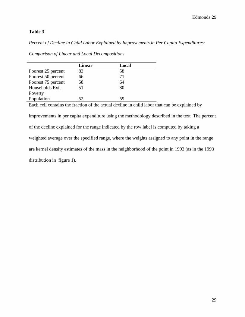
The standard linear model explains a remarkable fraction of the decline in child labor.

The first column of table 3 contains the results from the linear regression, and the second column

contains the equivalent of (8) calculated by replacing the linear expectations in the numerator

with the nonparametric expectations calculated in section III.C (figure 4). In the relatively

dispersed bottom quartile of the population, the linear estimator does better than the

nonparametric estimator, because the linear functional form solves the problems of low density

that plague the nonparametric regression. In the rest of the distribution, the local regression

techniques developed in this paper have greater explanatory power.

The difference between the local and linear results is greatest for households that exit

poverty. While the local regression techniques explain 80 percent of the decline in child labor

for this group, linear techniques explain only 51 percent of this group's decline. The reason for

this large difference between techniques in predicting declines in child labor for poverty exiting

households is evident in figure 2. There is a distinct change in slope and acceleration in the

decline in child labor associated with per capita expenditure for households in the neighborhood

of the poverty line in the local regression line for 1993 in figure 2. In households that exit

poverty between 1993 and 1998, per capita expenditure improve across this region of dramatic

declines in child labor. The linear regression misses this region of rapid decline in child labor,

Edmonds 21

21

and hence dramatically under-predicts the decline in child labor that occurs in households that

move out of poverty.

V. Conclusion

The main finding of this paper is that economic status improvements can explain much of

the dramatic decline in child labor that occurred in Vietnam during the 1990s. While child labor

declines in households throughout the per capita expenditure distribution, improvements in

economic status appear to explain the declines in child labor in poorer households more so than

in rich households. For households that emerge from poverty between 1993 and 1998, per capita

expenditure improvements can explain 80 percent of the observed decline in child labor.

These findings differ from much of the recent evidence on child labor and economic

status in four ways. First, the nonparametric tools used in this study allow for (and find)

important non-linearity in the correlation between economic status and child labor. Failing to

account for this non-linearity may lead to misleading results and conclusions. For example, in

Vietnam in 1993, I do not find that child labor is sensitive to economic status in the very poorest

and very richest households. If most households fell into one of those two regions of per capita

expenditure (in reality, they do not), then with parametric methods, I might conclude that there is

no link between economic status and child labor as does much of the recent empirical literature

on child labor and economic status.

Second, the relationship between economic status and child labor that explains the

decline in child labor through time is based on a single point in time. Hence, new technologies,

relative price shifts (including the market return to education), and policy, all factors likely to be

correlated with economic growth, by construction cannot be the source of the ability of

improvements in economic status to explain child labor. Thus, the results of this study provide a

Edmonds 22

22

rare piece of evidence linking the process of becoming richer to declines in child labor that is not

driven by the confounding factors that have drawn so much attention in the recent literature.

Third, the explanatory power of this paper comes from observing the same set of

households through time, rather than through comparing fundamentally different households.

Thus, the results of this study are based on within household declines in child labor explained by

within household changes in economic status. As a result, the findings of large reductions in

child labor associated with improvements in economic status reject theories that posit child labor

to be driven by preferences or norms that are invariant to the household's economic environment.

Fourth, I am not aware of any other study that examines how child labor responds to a

shift in the economic status distribution. This is of considerable policy interest. The process of

economic growth and international market integration may include shifts in the economic status

distribution of a county, and the empirical evidence on how households respond to this appears

to be virtually non-existent outside of the present study. If improvements in economic status do

not reduce child labor, then to the extent that child labor damages long-term human capital

accumulation, improvements in economic status may be transitory and unlikely to lead to long-

term or multi-generational improvements in household well-being. Long-term development

policy is then better focused on an activist social policy targeted to providing households with

incentives to keep children in school and out of work. On the other hand, if improvements in

economic status translate into decreases in child labor, then a more activist social policy may be

unnecessary. Resources may be better targeted to ameliorating the worst forms of child labor

and encouraging more immediate income generation. Further, punitive policies such as trade

sanctions designed to punish counties with high levels of child labor may actually increase child

labor if trade sanctions lower economic status.

Edmonds 23

23

I have ignored econometric issues associated with the effect of child labor on per capita

expenditure and with the joint determination of expenditure and the allocation of child time. To

interpret (4) as anything more than a conditional expectation, I would need a set of instruments

that impact expenditure per capita but not independently child time. This seems difficult in the

present case, because as is explicit in section III.B, anything that affects expenditure also affects

child labor supply. The consequence of the joint nature of per capita expenditure and child labor

for my analysis is that I cannot in general identify the mechanism through which the 1993 cross-

sectional relationship between per capita expenditure and child labor predicts child labor in 1998.

A natural question arises about how these results generalize. First, non-linearity in the

relationship between child labor and economic status appear very important. Much of the

growth in Vietnam between 1993 and 1998 appears to push household economic status across an

area of dramatic declines in child labor. I would hesitate to extrapolate from the results found

here to economic status levels outside of the data. Second, the growth in rural areas that took

place during the period of the panel appears to stem from agricultural liberalization and growth

in the productivity of the agriculture sector. Improvements in economic status from growth in

agriculture may have very different consequences for children than other types of growth. For

example, since 1999, Vietnam may have experienced a massive surge in small and medium sized

enterprises. This may result in additional, new earning opportunities for children. Whether

children take these earnings opportunities depends on the payoff the household perceives to

having the child work in these new enterprises. The household must weigh the disutility of

having the child work versus the additional income the child's work may bring. The contribution

of this paper is not to predict that the desire for less child work will dominate all additional

earnings opportunities. Rather, this paper shows that it is not inevitable that the need for

Edmonds 24

24

additional income will dominate even among the very poor households considered in this paper.

In fact, in the present case, improvements in economic status, even in the face of rising earnings

opportunities for child laborers, are associated with a very dramatic decline in child labor.

Works Cited

Acemoglu, Daron, and Joshua Angrist. 1999. “How Large are the Social Returns to Education? Evidence from Compulsory Schooling Laws.” NBER Working Paper 7444. Cambridge, Mass.: National Bureau of Economic Research.

Anand, Sudhir, and Martin Ravallion. 1993. "Human Development in Poor Countries: On the Role of Private Incomes and Public Services." Journal of Economic Perspectives. 7(1), 133-50.

Baland, Jean-Marie, and James A. Robinson. 2000. “Is Child Labor Inefficient?” Journal of Political Economy. August, 108(4), 663-79.

Basu, Kaushik. 1999. “Child Labor: Cause, Consequence, and Cure, with Remarks on International Labor Standards.” Journal of Economic Literature. 37(3), 1083-119.

Basu, Kaushik, and Pham Hoang Van. 1998. “The Economics of Child Labor.” American Economic Review, 88(3), 412-27.

Basu, Kaushik, and Zafiris Tzannatos. 2003. "The Global Child Labor Problem: What do we know and what can we do?" World Bank Economic Review. 17(2), 147-73.

Beegle, Kathleen, Rajeev H. Dehejia, and Roberta Gatti. 2003a. "Child Labor, Crop Shocks, and Credit Constraints." NBER Working Paper 10088. Cambridge, Mass.: National Bureau of Economic Research.

Beegle, Kathleen, Rajeev Dehejia, and Roberta Gatti. 2003b. Why should we care about child labor? New York: Columbia University Manuscript.

Ben-Porath, Yoram. 1967. "The Production of Human Capital and the Life Cycle of Earnings." Journal of Political Economy. 75(4), 352-65.

Bhalotra, Sonia, and Christopher Heady. 2003. "Child Farm Labor: The Wealth Paradox." World Bank Economic Review 17(2), 197-227.

Bommier, Antoine, and Pierre Dubois. 2003. "Rotten Parents and Child Labor." Journal of Political Economy. Forthcoming.

Boozer, Micheal, and Tanveet Suri. 2001. Child Labor and Schooling Decisions in Ghana. New Haven, CT: Yale University Manuscript.

Brown, Martin, Jens Christiansen, and Peter Phillips. 1992. “The Decline of Child Labor in the U.S. Fruit and Vegetable Canning Industry: Law or Economics?” Business History Review. 66, Winter, 723-70.

Edmonds 25

25

Brown, Drusilla, Alan Deardorff, and Robert Stern. 2003. "Child Labor: Theory, Evidence and Policy.” In K. Basu, H. Horn, L. Roman, and J. Shapiro, eds., International Labor Standards: History, Theories and Policy. Oxford: Basil Blackwell.

Deaton, Angus, and Christina Paxson. 1998. "Economies of Scale, Household Size, and the Demand for Food." Journal of Political Economy. 106(5), 897-930.

Deb, Partha. and Furio Rosati. 2002. "Determinants of Child Labor and School Attendance: The Role of Household Unobservables.” Understanding Children's Work Working Paper. December. Florence: Innocenti Research Center.

Edmonds, Eric. 2003. "Does Child Labor Decline with Improving Economic Status?" NBER Working Paper 10134. Cambridge, Mass.: National Bureau of Economic Research.

Edmonds, Eric, and Carrie Turk. 2004. "Child Labor in Transition." In P. Glewwe, N. Agrawal and D. Dollar, eds., Economic Growth, Poverty and Household Welfare: Policy Lessons from Viet Nam. Washington D.C.: World Bank

Emerson, Patrick M., and Souza, Andre Portela. (2003): "Is There a Child Labor Trap? Intergenerational Persistence of Child Labor in Brazil.” Economic Development and Cultural Change. 51(2), 375-98.

Ennew, Judith. 1982. “Family Structure, Unemployment, and Child Labour in Jamaica,” Development and Change. 13, 551-63.

Fan, Jianqing. and Irène Gijbels. 1995. Local Polynomial Modelling and Its Applications. New York: Chapman & Hall.

Fassa, Anaclaudia G. 2003. Health Benefits of Eliminating Child Labor. Geneva: International Labour Office.

Foster, Andrew D., and Mark R. Rosenzweig. 1996. "Technical Change and Human Capital Returns and Investments: Evidence from the Green Revolution." American Economic Review. 86(4): 931-53.

General Statistical Office. 1994. Viet Nam Living Standards Survey 1992-93. Ha Noi, Viet Nam.

General Statistical Office. 1999. Viet Nam Living Standards Survey 1997-98. Ha Noi, Viet Nam.

Glewwe, Paul., and Phong Nguyen. 2004. "Economic Mobility in Viet Nam in the 1990s." In P. Glewwe, N. Agrawal, and D. Dollar, eds., Economic Growth, Poverty and Household Welfare: Policy Lessons from Vietnam. Washington DC: World Bank.

Guarcello, Lorenzo, Fabrizia Mealli, and Furio Rosati. 2003. "Household Vulnerability and Child Labor: The Effect of Shocks, Credit Rationing, and Insurance." Understanding Children's Work Working Paper. July. Florence: Innocenti Research Center.

Hazan, Moshe, and Binyamin Berdugo. 2002. "Child Labor, Fertility, and Economic Growth." Economic Journal. 112(October): 810-28.

Heady, Christopher. 2003. “The Effect of Child Labor on Learning Achievement.” World Development. 31: 385–98.

Edmonds 26

26

Krueger, Alan B. 1997. "International Labor Standards and Trade." In M. Bruno and B. Pleskovic, eds., Annual World Bank Conference on Development Economics, 1996. Washington, D.C.: The World Bank. 281-302.

Levy, Victor. 1985. “Cropping Pattern, Mechanization, Child Labor, and Fertility in a Farming Economy: Rural Egypt.” Economic Development and Cultural Change. 33(4), 777-91.

Moehling, Carolyn. 1999. "State Child Labor Laws and the Decline of Child Labor." Explorations in Economic History, 36, 72-106.

Parsons, Donald O., and Claudia Goldin. 1999. "Parental Altruism and Self-Interest: Child Labor Among Late Nineteenth Century American Families." Economic Inquiry. 27(4): 637-59.

Paxson, Christina H. 1993. “Consumption and Income Seasonality in Thailand.” Journal of Political Economy. 101(1): 39-72.

Psacharopoulos, George. 1997. “Child Labor Versus Educational Attainment: Some Evidence from Latin America.” Journal of Population Economics. 10(4): 377-86.

Ranjan, Priya. 2001. “Credit Constraints and the Phenomenon of Child Labor.” Journal of Development Economics. 64(1): 81-102.

Ray, Ranjan. 2000. “Analysis of Child Labour in Peru and Pakistan: A Comparative Study.” Journal of Population Economics. 13(1): 3-19.

Rogers, Carol Ann, and Kenneth A. Swinnerton. 2001. Inequality, Productivity, and Child Labor: Theory and Evidence. Washington, D.C.: Georgetown University Manuscript.

Rogers, Carol Ann, and Kenneth A. Swinnerton. 2003. "Does Child Labor Decrease when Parental Incomes Rise," Journal of Political Economy. Forthcoming.

World Bank. 2000. Vietnam Living Standards Survey, 1997-98: Basic Information. Washington, D.C.: World Bank Poverty and Human Resources Division Manuscript.

World Bank and others. 1999. Vietnam Development Report 2000: Attacking Poverty. Joint Report of the Government-Donor-NGO Working Group, Hanoi.

Yang, Dean. 2003. Remittances and Human Capital Investments: Child Schooling and Child Labor in the Origin Households of Oversees Filipino Workers. Ann Arbor: University of Michigan Manuscript.

Edmonds 27

27

Table 1

Child Labor by Age and Through Time for Children

Percent of children participating in various types of work

1993 1998

Age Work Outside House Agriculture.

Family Business Work

Outside House Agriculture

Family Business

6 1.5 0.0 1.3 0.2 1.1 0.0 1.1 0.0 7 7.3 0.2 6.8 0.3 2.2 0.0 2.2 0.0 8 13.1 0.1 12.2 0.9 7.9 0.0 7.9 0.2 9 18.9 0.2 17.5 1.1 7.9 0.2 7.0 1.1 10 27.1 0.3 25 2.3 13.1 0.0 12.6 0.5 11 29.8 1.1 26.7 3.4 22.7 0.1 21.3 1.8 12 40.7 3.2 31.7 7.5 28.7 0.7 26.5 2.1 13 48.0 3.0 40.5 6.8 35.6 1.9 31.3 4.1 14 61.0 5.5 49.1 10.8 40.1 3.9 32.9 5.9 15 69.4 9.7 52.4 12.6 49.3 5.3 40.3 8.0 All means are weighted to be nationally representative for the indicated year. "Work" refers to

participation in the last 7 days in any of the indicated work categories. "Outside House"

indicates work outside of the child's household for pay (cash or in-kind). "Agriculture" indicates

work inside the child's own household in agricultural activities. "Family Business" refers to

work inside the child's own household in a family business or enterprise other than agriculture.

Edmonds 28

28

Table 2

Child Labor by Quintile of Per Capita Expenditure in 1993

Percent of children participating in various types of work, Panel Households Only

1993 1998

Quintile Work Outside House Agriculture

Family Business Work

Outside House Agriculture

Family Business

1 38.8 3.1 34.1 3.7 32 1.4 29 3.3 2 36.8 2.1 33.2 2.9 25.2 1.3 22.8 2.2 3 32.9 1.8 27.6 4.5 21.9 1.6 17.7 3 4 26.1 1.8 20.4 5.5 12.9 0.9 11.4 2 5 15.6 1.1 10.2 5.4 4.8 0.6 2.8 2 Quintiles are household quintiles of 1993 per capita expenditure. See table 2 for column

definitions.

Edmonds 29

29

Table 3

Percent of Decline in Child Labor Explained by Improvements in Per Capita Expenditures:

Comparison of Linear and Local Decompositions

Linear Local Poorest 25 percent 83 58 Poorest 50 percent 66 71 Poorest 75 percent 58 64 Households Exit Poverty

51 80

Population 52 59 Each cell contains the fraction of the actual decline in child labor that can be explained by

improvements in per capita expenditure using the methodology described in the text The percent

of the decline explained for the range indicated by the row label is computed by taking a

weighted average over the specified range, where the weights assigned to any point in the range

are kernel density estimates of the mass in the neighborhood of the point in 1993 (as in the 1993

distribution in figure 1).

Edmonds 30

30

Figure 1 The Distribution of Per Capita Expenditures in 1993 and 1998 Kernel density estimates

Edmonds 31

31

Figure 2 Child Labor by Per Capita Expenditure in 1993 Local regression results

Edmonds 32

32

Figure 3 Per Capita Expenditure in 1998 by Per Capita Expenditure in 1993 Local regression results

Edmonds 33

33

Figure 4 Explaining Changes in Child Labor with Changes in Per Capita Expenditure Decomposition (local regression) results

Edmonds 34

34

Figure 5 Declines in Child Labor by Per Capita Expenditure in 1993 and whether Per Capita Expenditures Increase or Decrease between 1993 and 1998 Limited to children in households with 1993 per capita expenditures that on average exit poverty between 1993 and 1998

Edmonds 35

35

1 Working children may bring income into the household and thereby ameliorate poverty.

Children may also learn skills while working that bring a return later in life (Beegle, Dehejia, and

Gatti 2003b). On the other hand, the presence of children in the labor market may depress wages

for adults and thereby create poverty (Basu and Van 1998). Moreover, child labor may conflict

with school attendance (for example, Boozer and Suri 2001), it may reduce the time children

invest in study and thereby school performance and attainment (as in Heady 2003), it may impair

child development through diminished play and leisure, and child labor may be associated with

worse health and nutritional status because of the environment in which children work (see Fassa

2003). Through these mechanisms, child labor may create an intergenerational poverty trap. For

formal presentations see Basu (1999), Emerson and Souza (2002), and Hazan and Berdugo

(2002).

2 This result follows from studies where child labor is a bad in parental preferences such as Basu

and Van (1998), Baland and Robinson (2000), Ranjan (2001), and Bommier and Dubios (2003).

Rogers and Swinnerton (2003) point out that rising incomes can increase child labor if credit

market imperfections induce parents to over-invest in education as a way of securing income for

parents in the future (via transfers from children).

3 One exception is the recent literature that has appeared subsequent to this paper that considers

how child labor supply is affected by economic shocks (Beegle, Dehejia, and Gatti 2003a,

Guarcello, Mealli, and Rosati 2003, Yang 2003) which generally finds child labor supply to be

responsive to unanticipated changes in the household's environment. While the response of child

labor supply to shocks depends on the operation of credit and insurance markets, there may also

be an income component in these studies.

Edmonds 36

36

4 A third interpretation is the Ben-Porath (1967) model where educational investments (and then

child labor supply) are determined by weighing the present discounted value of schooling against

its opportunity cost. If the equilibrium investment decision does not vary with economic status,

then child labor might not vary either. I have not seen this point raised as an interpretation of a

weak cross-sectional association between child labor and living standards.

5 The working paper version of this study extends the decomposition by looking at several

gender, age, and household size subgroups (Edmonds 2003). It also develops a semi-parametric

version of the methodology in section 3 in order to controls for differences in child labor that

vary with gender, age, and household size. The semi-parametric framework is also extend to

consider whether different assumptions about the calculation of adult equivalence scales affect

the predictive power of living standards.

6 Glewwe and Nguyen (2004) discuss attrition in the panel and conclude that the panel appears to

be approximately nationally representative. The panel recaptured 89.6 percent of its targeted

households. However, the reader should be cautioned that the experiences of panel households

might not generalize to the nation as a whole.

7 I divide total expenditure by household size to get total expenditure per capita. Implicit in

dividing by household size is a set of strong assumptions about the costs of children and

economies of scale within the household (Deaton and Paxson 1998). I consider this issue of

economies of scale in greater detail in the working paper version of this study (Edmonds 2003).

There are two justifications for looking at expenditure rather than income. First, most

households do not participate exclusively in formal labor markets. Hence, calculating income is

difficult. Second, while income is variable, households may try to smooth consumption

(represented in the VLSS by expenditure) through time. Evidence such as Paxson (1993)

Edmonds 37

37

suggests that expenditure varies less than income, and the life cycle hypothesis suggests

expenditure better reflects the household’s current beliefs about its long-term economic status.

8 Expenditure includes both purchased goods and the imputed value of home production that is

consumed in the household. Durable goods are not included in total expenditure, but an imputed

rental value of durables is included. Expenditure is deflated so that expenditure in both 1993 and

1998 is expressed in hundreds of January 1998 Dongs.

9 Measurement error in total expenditure is a chronic problem in expenditure surveys such as the

VLSS. The VLSS attempts to minimize measurement error by attaining expenditure information

separately on 64 food items and 86 nonfood items. However, measurement error in total

expenditure may hurt the ability of apparent per capita expenditure improvements to predict

declines in child labor, because some of the "improvements" might stem from measurement error

rather than changes in the household's economic environment.

10 In this discussion, I abstract from the question of how inequality affects child labor supply.

See Ranjan (2001) and Rogers and Swinnerton (2001) for in depth discussions.

11 The bandwidth selection procedure in figures 2-4 works as follows. I pick a bandwidth for the

point on the per capita expenditure grid with the greatest density. I then compute a bandwidth

for each point on the per capita expenditure grid by multiplying this bandwidth by the square of

the inverse of the estimated density (relative to the greatest observed density). The advantage of

this weighting is that the bandwidth used in estimating the expected incidence of child labor is

greater for parts of the per capita expenditure distribution with less mass. The base bandwidth

(at the point of greatest density) is selected by a cross-validation procedure that works as follows.

I consider a grid of possible bandwidths. For each bandwidth on the grid, I use the density based

procedure just described to compute a bandwidth for each point on the per capita expenditure

Edmonds 38

38

grid. I then compute the mean-integrated squared error across all observations. I repeat this

procedure across the range of bandwidths, and select the bandwidth that minimizes mean-

integrated squared error.

12 I estimate standard errors for the regression function by bootstrapping. The VLSS panel

consists of 3347 households with children drawn from 117 communes. Since there is likely

significant homogeneity in child labor within communes, the effective sample size is less than

3436. My bootstrapping procedure preserves this feature of the sample design by sampling

communes rather than households, then retaining all of the households within the selected

commune. I generate 100 such bootstrap samples and re-estimate the local regression for each

draw of the bootstrap.

13 Because the 1993 mapping (4) encounters support problems with the logarithm of per capita

expenditure in 1993 above 8.28, the 1998 predicted incidence of child labor can only be

computed for regions where the predicted per capita expenditure in 1998 is at or below 8.28.

Thus, the decomposition is limited to households with a 1993 logarithm of per capita expenditure

of 8.07 or less, because the predicted per capita expenditure in 1998 for households with a 1993

log pcx of 8.07 is 8.28. All remaining figures are then pictured with a range of 6.51 to 8.07.

14 I calculate the fraction of the decline in child labor that can be explained by living standards

improvements by calculating the fraction of the decline in child labor explained by the predicted

line for each point on the per capita expenditure grid. I then take the weighted average of these

fractions using kernel density estimates of the 1993 per capita expenditure distribution.

15 An observationally equivalent explanation would come from a model with continuous child

labor supply and an Engel curve for food in family preferences. I am grateful to Andrew Foster

for pointing this out.

Edmonds 39

39

16 There is an obvious endogeneity problem in this bifurcation. If a child exogenously stops

working, then per capita expenditures may decline. Hence, it is plausible that declines in child

labor will be concentrated in households that experience declines in per capita expenditure

17 This regression estimates 1,93β as –0.13; the t-statistics is 12.08 for the test of the null-

hypothesis that 1,93β is 0.