DP2015-23

Does Agricultural Growth Reduce

Inequality and Poverty in Developing Countries?*

Katsushi S. IMAI Raghav GAIHA Wenya CHENG

Revised April 4, 2016

* The Discussion Papers are a series of research papers in their draft form, circulated to encourage discussion and comment. Citation and use of such a paper should take account of its provisional character. In some cases, a written consent of the author may be required.

1

Does Agricultural Growth Reduce Inequality and Poverty in Developing

Countries?

Katsushi S. Imai*

Raghav Gaiha**

Wenya Cheng***

*School of Social Sciences, University of Manchester, UK & RIEB, Kobe University, Japan

**Faculty of Management Studies, University of Delhi, India, & Global Aging Program,

Harvard School of Public Health, Harvard University Boston, USA *** School of Social Sciences, University of Manchester, UK

This Draft: 4th April 2016

Abstract

Drawing upon cross-country panel data for developing countries, the present study examines

the role of agricultural growth in reducing inequality and poverty by modelling the dynamic

linkage between agricultural and non-agricultural sectors. For this purpose, we have

compared the role of agricultural growth and that of non-agricultural growth and have found

that agricultural growth is more important in reducing poverty, while the negative effect of

agricultural growth on inequality is found in a few models where specific definitions of

inequality are adopted. The role of agricultural growth in reducing inequality is, however,

undermined by ethnic fractionalisation which tends to make inequality more persistent. Our

analysis generally reinforces the case for revival of agriculture in the post-2015 discourse,

contrary to the much emphasised roles of rural-urban migration and urbanisation as main

drivers of growth and elimination of extreme poverty.

Keywords: Inequality, Poverty, Growth, Agriculture, Non-agriculture, MDG, SDG

JEL Codes: C20, I15, I39, O13

Corresponding Author:

Katsushi Imai (Dr)

Economics, School of Social Sciences

University of Manchester, Arthur Lewis Building,

Oxford Road, Manchester M13 9PL, UK

Phone: +44-(0)161-275-4827 ; Fax: +44-(0)161-275-4928

E-mail: Katsushi.Imai@manchester.ac.uk

Acknowledgements

Authors are grateful to Thomas Elhaut, Director (on sabbatical), IFAD, for his enthusiastic support and

guidance throughout this study and for his insistence on highest standards of analytical rigour. They also

thank Adams Sorekuong Adama and Abdi Ali for providing the price uncertainty data of export prices.

The second author acknowledges David Bloom’s support and advice in the initial stage of this study. The

views expressed are personal and not necessarily of the organisations to which we are affiliated.

2

Does Agricultural Growth Reduce Inequality and Poverty in Developing

Countries?

1. Introduction

The main objective of this study is to examine the role of agricultural growth in reducing

inequality and poverty using cross-country panel data for developing countries. To achieve this

objective, we compare the roles of agricultural growth and non-agricultural growth in poverty

and inequality reduction by modelling the linkage between agricultural and non-agricultural

sectors. Both poverty headcount ratios and poverty gaps are used as measures of poverty. More

broadly, we aim to re-establish the role of agricultural growth - mainly because recent studies by

the World Bank (e.g. The Global Monitoring Report 2013 (World Bank, 2013)) and others have

questioned the primacy of agricultural growth in stimulating overall growth and reduction of

poverty.1 As a persuasive case for stimulating agricultural growth and poverty reduction was

made by World Development Report 2008 (World Bank, 2007), it is necessary to examine it in

light of more recent evidence. Given the goal of elimination of extreme poverty by 2030, and the

lively discourse on the post-2015 development agenda, a careful determination of sectoral

growth priorities is imperative.

It is claimed by the World Bank (2013) and Chandy et al. (2011), among others, that the

Millennium Development Goal (MDG) 1A2 of halving extreme poverty by 2015 was achieved in

1 In this context Collier and Dercon (2014) have questioned the role of smallholders in African

development. Because of the data limitation, the present study focuses on the growth of overall

agricultural sector growth - rather than the growth originating from smallholders - on poverty and

inequality. 2 MDG1A refers to “Millennium Development Goal, Target 1.A”, “Halve, between 1990 and 2015, the

proportion of people whose income is less than $1.25 a day”

(http://www.un.org/millenniumgoals/poverty.shtml). This has led to Sustainable Development Goal

(SDG) is “By 2030, eradicate extreme poverty for all people everywhere, currently measured as people

living on less than $1.25 a day” (https://sustainabledevelopment.un.org/sdg1).

3

2010 – five years ahead of the deadline. Yet 970 million will remain poor in 2015, with 84 per

cent concentrated in South Asia and Sub-Saharan Africa. The latter is also the only region that

was expected not to achieve MDG 1A by 2015. It should also be noted that global poverty

remains a rural problem with more than three-fourths of the extremely poor located in rural

areas. However, as global poverty fell, so did the gap between rural-urban poverty. It reduced by

half in East Asia and the Pacific by 2008, while in Sub-Saharan Africa, Latin America and the

Caribbean, and South Asia, there was less progress. World Bank (2013) also makes an important

contribution to the discourse on MDGs by disaggregating progress into rural and urban

components. In doing so, it offers striking examples of the continuing rural-urban disparities in

several MDGs. It does not, however, disaggregate the 970 million that remained in extreme

poverty in 2015 into those who were in rural and urban areas, respectively. This is crucial for

designing appropriate policy interventions for rural and urban areas.

World Bank (2013) makes a powerful case for rapid and efficient urbanisation as key to

overall poverty reduction. It rests on better utilisation of agglomeration economies and efficient

rural-urban migration. Indeed, it is argued that these could also result in speedier rural poverty

reduction. An important link in the chain is small cities (somewhat controversially referred to as

“the missing middle”). Their weak infrastructure, and poor hygiene and sanitation are likely to

turn them into slums with growing rural-urban migration. So the refrain is that investment must

be directed to such cities to better exploit their growth potential.

Curiously, rural-urban migration contributing 40 per cent of the increase in urban population

over the period 2010-2030 has two sides to it. One is the poverty reduction through the growth of

small cities and rapid urbanisation. The premise is that more rural-urban migration will have a

substantial payoff in terms of higher wages of those who stay in rural areas, and greater

4

diversification of rural economies. If this is turned on its head, it could be argued that more

efficient land, labour and credit markets and better infrastructure in rural areas would not only

help raise agricultural productivity, but also enable diversification of rural economies. In

particular, the dynamic between farm and non-farm activities has assumed greater significance

with the diversification of the former (Thapa and Gaiha, 2014). Non-farm activities are not just

remunerative but also help stabilise rural incomes. Consequently, the rapid pace of rural-urban

migration - highest in Latin America and the Caribbean and lowest in South Asia and Sub-

Saharan Africa - will slowdown. Better and more diversified livelihood opportunities in rural

areas cannot be discarded as the inferior option relative to the more rapid and efficient

urbanisation thesis with considerable risks of uncontrollable growth of slums with pervasive

multiple deprivations (malnutrition and infectious diseases).

Much of sustained reduction in poverty hinges on how growth and inequality interact - a

subject that has gained prominence in a context of rising inequality in a large part of the

developing world in the last two decades. As argued in a recent UN report (United Nations,

2013), addressing inequality is not just a moral imperative but a necessity for sustainable

development3. Evidence points to the powerful and corrosive effects of inequality on poverty

reduction, social cohesion and stability. A major part of the solution lies in fostering inclusive

and sustainable rural transformation through a comprehensive approach to food security and

nutrition, addressing the linkages between agriculture, health, education, water, energy, gender

equity and poverty. Both poverty and inequality reduction are clearly featured in the Sustainable

3 As noted by Doyle and Stiglitz (2014), “There are ….substantial links between violence and “horizontal

inequalities” that combine economic stratification with race, ethnicity, religion or region. When the poor

are from one race, ethnicity, religion or region, and the rich are from another, a lethal destabilizing

dynamic often emerges” (p.8).

5

Development Goals (SDGs), or the 2030 Agenda for Sustainable Development, which were

agreed at United Nations Sustainable Development Summit 2015 in September 2015.

The present study departs from the extant literature in the following ways. First, as an

extension of Christiaensen et al. (2011), we will estimate the dynamic linkages between

agricultural growth and non-agricultural growth using a dynamic panel model applied to cross-

county panel data (Blundell and Bond, 1998)4. We will apply this model separately for non-

agricultural sector growth and agricultural sector growth in which both lagged agricultural

growth and lagged non-agricultural growth are used as explanatory variables in each model after

taking account of the endogeneity of the past growth of both sectors. This will enable us to

estimate effects from the non-agricultural sector to the agricultural sector, and vice versa. For

instance, the improvement in productivity in the agricultural sector (e.g. through the shift from

basic staple food production to high yield varieties or non-staple food production) is likely to

have positive effects on non-agricultural growth, while the non-agricultural sector growth may

impact the agricultural sector through the change in demand patterns for primary goods.5 Second,

we will apply Pesaran’s (2006) common correlated effects mean group (CCEMG) estimator to

take account of the cross-country dependence of error terms. This model has an advantage in

obtaining the time-series regression estimate for each country with the shocks common to all the

countries. Third, we will estimate the effects of agricultural and non-agricultural growth terms as

predictions of the dynamic panel model on inequality and poverty. This focuses on the dynamic

role of agricultural growth -in comparison with that of non-agricultural growth - in reducing not

4 It is referred to as system generalized method of moments (SGMM) estimator which enables us to

model the dynamics of agricultural growth and non-agricultural growth over time. 5 See Christiaensen et al. (2011) and de Janvry and Sadoulet (2010) for more detailed discussions on the

linkages between these sectors.

6

only poverty, but also inequality. We have thus extended Christiaensen et al. (2011) by using

different models and more recent data, including the comprehensive data on inequality.

The rest of the paper is structured as follows. After briefly reviewing the literature in Section

2, we summarises the data sources in Section 3. Section 4 elaborates the econometric models we

will employ. Regression results are discussed in Section 5. Section 6 offers concluding remarks

with policy implications.

2. The Literature Review

Despite the large body of literature demonstrating the role of agricultural growth in overall

economic growth and poverty,6 rigorous empirical analyses of the role of growth in both

agricultural and non-agricultural sectors and their interactions are still few and far between, with

a few exceptions such as Haggblade and Hazell (1989), Haggblade et al. (2007), de Janvry and

Sadoulet (2010) and Christiaensen et al. (2011). Haggblade and Hazell (1989) used cross-country

data (43 countries) and illustrated the close interaction between these sectors, based on statistical

comparisons of agricultural income and non-farm sector employment share. Haggblade et al.

(2007) reported large multiplier or indirect effect from agricultural sector to non-agricultural

sector.7 de Janvry and Sadoulet (2010) reviewed several empirical studies, including their own

on China and Vietnam, that confirm substantial sectoral linkages and their poverty reduction

potential. They used time-series estimations (based on VAR model) for China in 1980-2001 and

showed that non-agricultural growth has a substantial indirect effect on agricultural growth (p.8).

Using the household panel data on Vietnam in the 1990s, they also showed that agricultural

6 See de Janvry and Sadoulet (2010) or Chistiaensen et al. (2011) for a review of the literature.

7 Haggblade et al. (2007) give evidence on multiplier effects of agricultural sector using an input-output

model for developing countries.

7

households with more market access experienced the faster pace of poverty reduction than

subsistence- oriented households (p.16).

Chistiaensen et al. (2011) is the first rigorous work to estimate the dynamic linkages between

agricultural growth and non-agricultural growth as well as those between these sectoral growth

components and poverty, drawing upon a cross-country panel dataset. They applied a dynamic

panel model to take into account the dynamic realisation of agricultural growth (or non-

agricultural growth) by having lagged dependent variables, while considering the dynamic effect

of non-agricultural growth (or agricultural growth) on agricultural growth (or non-agricultural

growth) over time. Their estimation strategy (SGMM) is based on Arellano and Bover (1995)

and Blundell and Bond (1998) with the finite sample correction of the two-step standard errors

proposed by Windmeijer (2005). The present analysis also uses the Blundell and Bond estimator

with the Windmeijer correction. More specifically, our model consists of two stages where in the

first stage agricultural (or non-agricultural) growth is estimated by non-agricultural (or

agricultural) growth and, in the second, inequality (or poverty) is estimated by (predicted) values

of agricultural and non-agricultural growth.

3. Data

The data for the first set of analyses of the effects of agricultural and non-agricultural growth on

inequality or poverty in Section 2 are mainly based on World Development Indicators (WDI)

2011, 2012, 2013 and 2014 (e.g. World Bank, 2014). The data on education and a few other

variables are based on Barro and Lee (2010). To construct the proxy for institutional qualities,

we have used the World Bank’s World Governance Indicators

(http://info.worldbank.org/governance/wgi/index.asp). We have derived the simple average of

8

four indicators, voice and accountability, political stability and absence of violence, rule of law

and control of corruption to capture the overall quality of institutions. While Christiaensen et al.

(2011) uses the three year averaged data over the period 1960–2005 for a sample of 85 countries

and 588 observations in their main specification (the columns (1) of Table 3 in Christiaensen et

al.), the present study covers the period 1969-2010 for 59 countries and 532 observations (Case

1, Table 1). The list of countries is given in Appendix 1. The difference is due to the fact that we

have updated the data and have used a different set of explanatory variables.

We will adopt three kinds of inequality measures. First, following Herzer and Vollmer’s

(2012) work which estimated the relationship between economic growth and inequality, we have

used the inequality data based on the EHII data - derived from the relationship between UTIP-

UNIDO, other conditioning variables, and the World Bank's Deininger and Squire data set. This

is taken from the University of Texas Inequality Project (http://utip.gov.utexas.edu/data.html).

Herzer and Vollmer (2012) selected 46 countries for the period 1970-2008 to minimise the

problem of missing observations given that they apply the panel co-integration method. The

EHII dataset is based on Theil’s T statistic measured across sectors within each country where

the classifications of sectors are standardized, based on UNIDO’s Industrial Statistics and

Eurostat to facilitate international comparisons. While we use the EHII data on inequality, it will

not be sufficient to use the data for only 18 developing countries, as in Herzer and Vollmer

(2012), for the purpose of deriving any useful policy implications for developing countries.

Apart from policy considerations, it may not be appropriate either - as a serious empirical work

to test economic theories - to pool both developed and developing countries overlooking the

structural difference between developed and developing economies (e.g. incomplete credit and

insurance markets in the latter). We have thus constructed an unbalanced panel data for

9

inequality based on the EHII data covering a larger number of countries (86 countries) for a

longer period (1970-2008). Besides, we have further expanded the EHII data on inequality by

supplementing them with the World Bank data (World Bank, 2014) on inequality (the Gini

Index) on the PovcalNet, by estimating the EHII data on inequality by the World Bank data

(World Bank 2014) using Ordinary Least Squares and replacing the missing observations by the

‘out-of-sample’ predictions. With this method, we have managed to cover 119 countries,

including 49 countries8 in the first set of analyses.

9 While the data quality and comparability are

not ideal, this method has the advantage of covering more countries (about six times more

developing countries than in Herzer and Vollmer (2012)). While the UTIP-UNIDO dataset on

pay inequality is based on global pay inequality data, Galbraith and Kum (2005) have shown that

this is highly correlated with the Deininger and Squire’s (1996) Gini measure of inequality and it

is thus reasonable to assume that the EHII dataset is one of the best data sources for inequality

analyses of developing countries in terms of its coverage of countries. In our case coefficient of

correlation between the EHII data on inequality and the Gini coefficient is 0.723. However, the

limitation of the EHII dataset should be noted as it does not cover self-employment data or the

agricultural wage data and may be a poor proxy for inequality of low income countries relying

on agricultural sectors. Second, given the limitations of the EHII dataset, we will also use the

World Bank’s Gini index. While this is widely used, a major limitation of the Gini index in our

study context is that the coverage of countries/years is highly limited. We cannot thus apply

Pesaran’s CCEMG model. Third, we will also use the ‘raw’ EHII data of inequality without

aforementioned adjustment. In this case the coverage of years/countries is also limited. Although

8 The number of countries varies from 40 to 49 depending on which specification we use for the

inequality estimation. 9 Descriptive statistics are found in Appendix 2.

10

each indicator has its own limitations, we will apply these three measures in our empirical

analyses.

4. Econometric Models

1st Stage: estimation of non-agricultural growth and agricultural growth

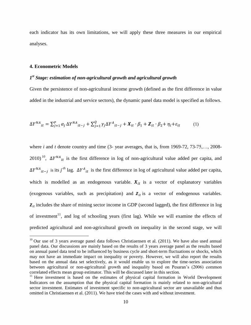
Given the persistence of non-agricultural income growth (defined as the first difference in value

added in the industrial and service sectors), the dynamic panel data model is specified as follows.

∆𝑌𝑁𝐴𝑖𝑡 = ∑ 𝛼𝑗

𝑃𝑗=1 ∆𝑌𝑁𝐴

𝑖𝑡−𝑗 + ∑ 𝛾𝑗∆𝑌𝐴𝑖𝑡−𝑗

𝑄𝑗=1 + 𝑿𝑖𝑡 ∙ 𝛽1 + 𝒁𝑖𝑡 ∙ 𝛽2+ 𝜂𝑖+𝜀𝑖𝑡 (1)

where i and t denote country and time (3- year averages, that is, from 1969-72, 73-75,…, 2008-

2010) 10

, ∆𝑌𝑁𝐴𝑖𝑡 is the first difference in log of non-agricultural value added per capita, and

∆𝑌𝑁𝐴𝑖𝑡−𝑗 is its j

-th lag. ∆𝑌𝐴

𝑖𝑡 is the first difference in log of agricultural value added per capita,

which is modelled as an endogenous variable. 𝑿𝑖𝑡 is a vector of explanatory variables

(exogenous variables, such as precipitation) and 𝒁𝑖𝑡 is a vector of endogenous variables.

𝒁𝑖𝑡 includes the share of mining sector income in GDP (second lagged), the first difference in log

of investment11

, and log of schooling years (first lag). While we will examine the effects of

predicted agricultural and non-agricultural growth on inequality in the second stage, we will

10

Our use of 3 years average panel data follows Christiaensen et al. (2011). We have also used annual

panel data. Our discussions are mainly based on the results of 3 years average panel as the results based

on annual panel data tend to be influenced by business cycle and short-term fluctuations or shocks, which

may not have an immediate impact on inequality or poverty. However, we will also report the results

based on the annual data set selectively, as it would enable us to explore the time-series association

between agricultural or non-agricultural growth and inequality based on Pesaran’s (2006) common

correlated effects mean group estimator. This will be discussed later in this section. 11

Here investment is based on the estimates of physical capital formation in World Development

Indicators on the assumption that the physical capital formation is mainly related to non-agricultural

sector investment. Estimates of investment specific to non-agricultural sector are unavailable and thus

omitted in Christiaensen et al. (2011). We have tried the cases with and without investment.

11

insert the (endogenous) inequality in one of the specifications to see whether inequality has any

impact on non-agricultural growth. In one specification, we have interacted ∆𝑌𝐴𝑖𝑡with the Sub-

Saharan African dummy (SSA) to see if the effect of agricultural growth on non-agricultural

growth is different in SSA and elsewhere, following Christiaensen et al. (2011). 𝜂𝑖 is the

country-specific unobservable (e.g. social and cultural factors) and 𝜀𝑖𝑡 is an error term,

independent, and identically distributed (or i.i.d.).

As an alternative to the standard first differencing approach12

13

, we can use the lagged

differences of all explanatory variables as instruments for the level equation and combine the

difference equation (1) and the level equation (that is, the equation where ∆𝑌𝑁𝐴𝑖𝑡 is replaced by

𝑌𝑁𝐴𝑖𝑡 in equation (1)) in a system. Here the panel estimators use instrumental variables based on

previous realisations of the explanatory variables as the internal instruments, using the Blundell-

Bond (1998) system GMM (SGMM) estimator based on additional moment conditions. Such a

system gives consistent results under the assumptions that there is no second order serial

correlation and the instruments are uncorrelated with the error terms. The Blundell-Bond System

GMM (SGMM) estimator is used in the present study. This estimator is useful to address the

12

Two issues have to be resolved in estimating the dynamic panel model. One is endogeneity of the

regressors and the second is the correlation between(∆𝑌𝑖𝑡−1 − ∆𝑌𝑖𝑡−2) and (𝜀𝑖𝑡−𝜀𝑖𝑡−1) (e.g. see Baltagi,

2005). Assuming that 𝜀𝑖𝑡 is not serially correlated and that the regressors in 𝑿𝑖𝑡 are weakly exogenous, the

generalized method-of-moments (GMM) first difference estimator (e.g. Arellano and Bond, 1991) can be

used. It should also be noted that, as Hayakawa (2007) has shown by simulations for various cases (e.g.

n=50), the possible biases for small sample are smaller with the SGMM estimator than with the GMM

first-difference estimator. We have thus adopted the SGMM estimator to minimise the biases. 13

We have presented Arellano-Bond test for zero autocorrelation in first-differenced errors and Sargan

test of overidentifying restrictions for each table. In most cases, the results of the former show the first-

order correlations of the first differenced errors which justify including the one-period lagged dependent

variable. Considering the fact that 𝒁𝑖𝑡, endogenous variables - which are instrumented by their own lags -

tend to be persistent over time and thus Sargan test rejects the null hypothesis that over-identifying

restrictions are valid in some cases (i.e., Cases 1, 3, 4, 5 and 6 of Table 1, Case 5 of Table 3, and Cases 1

and 7 of Table 4) and the results in these cases should be interpreted with caution. Over-identifying

restrictions are deemed valid in other cases (i.e., Case 2 of Table 1, all the cases of Table 2, Cases 1, 2, 3,

4, and 6 of Table 3, and Cases 2 and 8 of Table 4). Using different specifications (e.g. including external

instruments, treating 𝒁𝑖𝑡 as exogenous) does not overcome this difficulty.

12

problem of endogenous regressors, 𝒁𝑖𝑡 (e.g. lagged agricultural growth in equation (1)). In the

system of equations, endogenous variables can be treated similarly to lagged dependent

variables. The second lagged levels of endogenous variables could be specified as instruments

for the difference equation. The first lagged differences of those variables could also be used as

instruments for the level equation in the system.

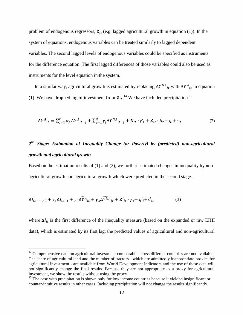
In a similar way, agricultural growth is estimated by replacing ∆𝑌𝑁𝐴𝑖𝑡 with ∆𝑌𝐴

𝑖𝑡 in equation

(1). We have dropped log of investment from 𝒁𝑖𝑡.14

We have included precipitation.15

∆𝑌𝐴𝑖𝑡 = ∑ 𝛼𝑗

𝑃𝑗=1 ∆𝑌𝐴

𝑖𝑡−𝑗 + ∑ 𝛾𝑗∆𝑌𝑁𝐴𝑖𝑡−𝑗

𝑄𝑗=1 + 𝑿𝑖𝑡 ∙ 𝛽1 + 𝒁𝑖𝑡 ∙ 𝛽2+ 𝜂𝑖+𝜀𝑖𝑡 (2)

2nd

Stage: Estimation of Inequality Change (or Poverty) by (predicted) non-agricultural

growth and agricultural growth

Based on the estimation results of (1) and (2), we further estimated changes in inequality by non-

agricultural growth and agricultural growth which were predicted in the second stage.

∆𝐼𝑖𝑡 = 𝛾0 + 𝛾1∆𝐼𝑖𝑡−1 + 𝛾2∆𝑌�̂�𝑖𝑡 + 𝛾3∆𝑌𝑁�̂�

𝑖𝑡 + 𝒁′𝑖𝑡 ∙ 𝛾4+ 𝜂′𝑖+𝜀′𝑖𝑡 (3)

where ∆𝐼𝑖𝑡 is the first difference of the inequality measure (based on the expanded or raw EHII

data), which is estimated by its first lag, the predicted values of agricultural and non-agricultural

14

Comprehensive data on agricultural investment comparable across different countries are not available.

The share of agricultural land and the number of tractors - which are admittedly inappropriate proxies for

agricultural investment - are available from World Development Indicators and the use of these data will

not significantly change the final results. Because they are not appropriate as a proxy for agricultural

investment, we show the results without using the proxy. 15

The case with precipitation is shown only for low income countries because it yielded insignificant or

counter-intuitive results in other cases. Including precipitation will not change the results significantly.

13

growth (∆𝑌�̂�𝑖𝑡 and ∆𝑌𝑁�̂�) as well as a vector of endogenous variables, 𝒁′𝑖𝑡 , such as, log of

schooling years and political stability which is taken from the World Bank’s World Governance

Indicators. This is estimated by the Blundell-Bond system GMM estimator with the finite-sample

correction. The equation is estimated by the fixed effects model with the robust estimator for the

Gini coefficient due to small sample size.

While the determinants of inequality or its changes have been analysed theoretically as well

as empirically in the macro and development economics literature, there is no single consensus,

as far as we aware, as to what sort of models should be used for inequality or its change. The

earlier theoretical literature draws upon Kuznets’s (1955, 1963) hypothesis of the inverted U

relation between inequality and GDP per capita. Under the hypothesis, at the initial stage of

development, inequality increases as GDP per capita increases, for instance, as (i) the rural-urban

inequality gap as well as (ii) the inequality within the urban sector increases. This is caused by

rural-to-urban migration as urban areas are industrialised, while urban wage workers’ pay rise

does not match the increase in profits of capital owners. While the agricultural sector features

low per capita income and relatively little inequality within the sector (Barro, 2000), in the

process of development, the inequality within rural sector may increase while the agricultural

sector reduces its size, in which only a subset of households are likely to benefit from

mechanisation and/or rural-to-urban migration. Under these circumstances, both agricultural and

non-agricultural growth is likely to increase inequality at the early stage of development.

However, inequality is supposed to decrease after a significant number of people benefit from

industrialization.16

More recently, Acemoglu and Robinson (2002) proposed a political economy

16

While the empirical literature on Kuznets hypothesis typically tests signs of a square and a cube of

GDP per capita to examine the inverted U relationship between inequality and GDP per capita, we do not

include these terms as this is not our primary objective. In most specifications, squared agricultural and

non-agricultural terms are found to be statistically insignificant.

14

model of the Kuznets Curve where they emphasised the role of political stability and

democratisation, leading to institutional changes and thus redistribution. In Barro’s (2000)

specification for inequality, he controlled for not only log GDP per capita, but also schooling and

political and institutional indices. On the other hand, Bourguignon and Morrisson (1998)

modelled the inequality being determined by the relative labour productivity of non-agricultural

and agricultural sectors. Our empirical specification draws upon Bourguignon and Morrisson

(1998) as well as Barro (2000), but we have adopted a simplified version as Equation (3) guided

by the data availability.17

As an extension, we have also applied Pesaran’s (2006) common correlated effects mean

group (CCEMG) estimator. This estimator enables us to model the country-level heterogeneity in

estimating the relationship between inequality change and agricultural/non-agricultural growth. It

also corrects for the cross-sectional correlations of unobservable factors that change over time.

These two points are recent developments in the panel data econometrics to overcome the

limitations of the standard fixed effects model where the country-level heterogeneity is ignored

and the unobservable factors are fixed without allowing correlations across different units (or

countries). However, the data requirement for the CCEMG model is large as it requires a

relatively large t (number of years) and i (number of countries) and we have thus applied this

model only for the annual panel data in the case we use the expanded EHII data on inequality.

Another useful feature of CCEMG model is to enable us to derive the coefficient estimate for

each country by utilising both time-series variation for the country and the factors common

across different countries. This provides us with the coefficient estimate for each country to

17

Ideally, we should model the effect of sectoral growth on sectoral inequality, that is, inequality within

agricultural or non-agricultural sector (or rural or urban sector) in Equation (3). However, we use an

aggregate inequality of the country (𝐼𝑖𝑡) as such data are not available.

15

show how the linkages between inequality change and agricultural (or non-agricultural) growth

differ across countries. We then apply OLS to estimate the underlying determinants for them by

simply regressing the saved coefficient on exogenous variables. As a base line of the CCEMG

model, the MG (mean group) model (Pesaran and Smith, 1995) is estimated whereby the

country-level heterogeneity is modelled without correcting for the cross-sectional correlations of

unobservable factors that change over time.

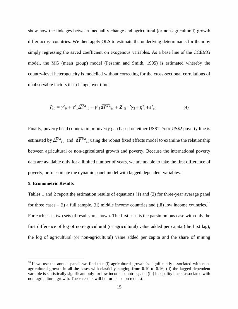
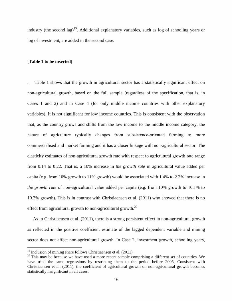
𝑃𝑖𝑡 = 𝛾′0 + 𝛾′1∆𝑌�̂�𝑖𝑡 + 𝛾′2∆𝑌𝑁�̂�

𝑖𝑡 + 𝒁′𝑖𝑡 ∙ ′𝛾3+ 𝜂"𝑖+𝜀"𝑖𝑡 (4)

Finally, poverty head count ratio or poverty gap based on either US$1.25 or US$2 poverty line is

estimated by ∆𝑌�̂�𝑖𝑡 and ∆𝑌𝑁�̂�

𝑖𝑡 using the robust fixed effects model to examine the relationship

between agricultural or non-agricultural growth and poverty. Because the international poverty

data are available only for a limited number of years, we are unable to take the first difference of

poverty, or to estimate the dynamic panel model with lagged dependent variables.

5. Econometric Results

Tables 1 and 2 report the estimation results of equations (1) and (2) for three-year average panel

for three cases – (i) a full sample, (ii) middle income countries and (iii) low income countries.18

For each case, two sets of results are shown. The first case is the parsimonious case with only the

first difference of log of non-agricultural (or agricultural) value added per capita (the first lag),

the log of agricultural (or non-agricultural) value added per capita and the share of mining

18

If we use the annual panel, we find that (i) agricultural growth is significantly associated with non-

agricultural growth in all the cases with elasticity ranging from 0.10 to 0.16; (ii) the lagged dependent

variable is statistically significant only for low income countries; and (iii) inequality is not associated with

non-agricultural growth. These results will be furnished on request.

16

industry (the second lag)19

. Additional explanatory variables, such as log of schooling years or

log of investment, are added in the second case.

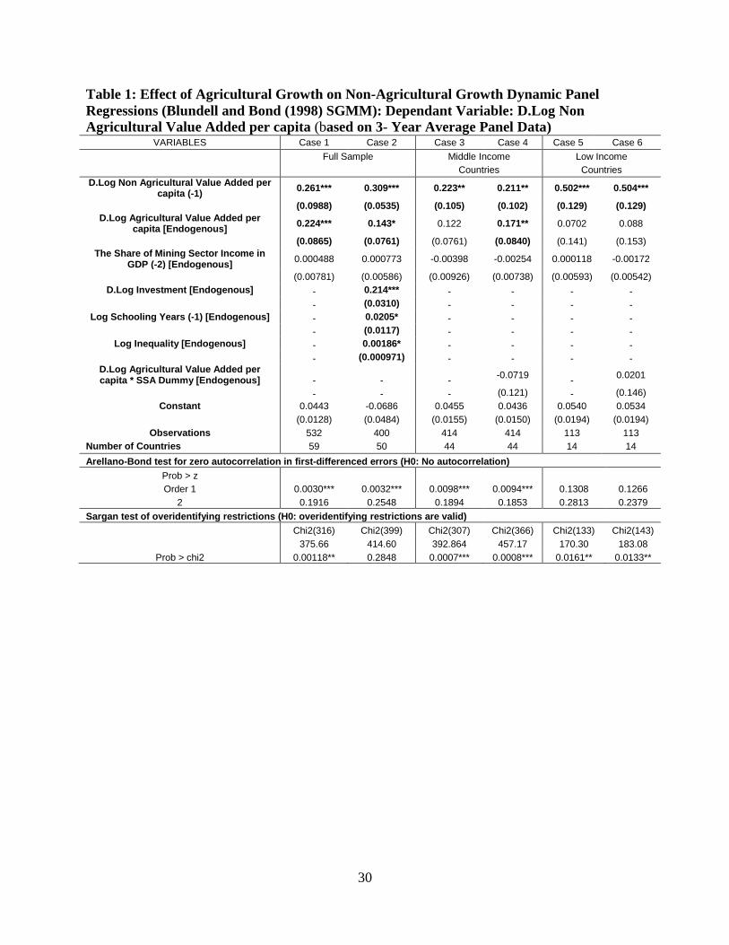
[Table 1 to be inserted]

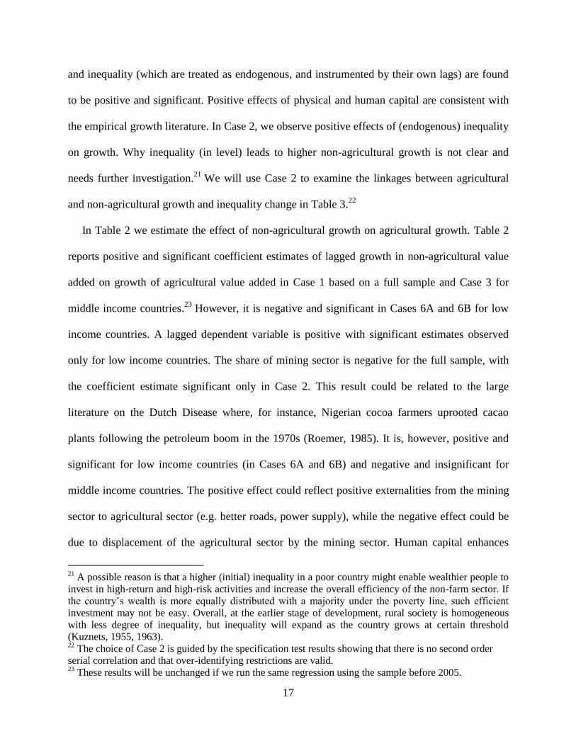
. Table 1 shows that the growth in agricultural sector has a statistically significant effect on

non-agricultural growth, based on the full sample (regardless of the specification, that is, in

Cases 1 and 2) and in Case 4 (for only middle income countries with other explanatory

variables). It is not significant for low income countries. This is consistent with the observation

that, as the country grows and shifts from the low income to the middle income category, the

nature of agriculture typically changes from subsistence-oriented farming to more

commercialised and market farming and it has a closer linkage with non-agricultural sector. The

elasticity estimates of non-agricultural growth rate with respect to agricultural growth rate range

from 0.14 to 0.22. That is, a 10% increase in the growth rate in agricultural value added per

capita (e.g. from 10% growth to 11% growth) would be associated with 1.4% to 2.2% increase in

the growth rate of non-agricultural value added per capita (e.g. from 10% growth to 10.1% to

10.2% growth). This is in contrast with Christiaensen et al. (2011) who showed that there is no

effect from agricultural growth to non-agricultural growth.20

As in Christiaensen et al. (2011), there is a strong persistent effect in non-agricultural growth

as reflected in the positive coefficient estimate of the lagged dependent variable and mining

sector does not affect non-agricultural growth. In Case 2, investment growth, schooling years,

19

Inclusion of mining share follows Christiaensen et al. (2011). 20

This may be because we have used a more recent sample comprising a different set of countries. We

have tried the same regressions by restricting them to the period before 2005. Consistent with

Christiaensen et al. (2011), the coefficient of agricultural growth on non-agricultural growth becomes

statistically insignificant in all cases.

17

and inequality (which are treated as endogenous, and instrumented by their own lags) are found

to be positive and significant. Positive effects of physical and human capital are consistent with

the empirical growth literature. In Case 2, we observe positive effects of (endogenous) inequality

on growth. Why inequality (in level) leads to higher non-agricultural growth is not clear and

needs further investigation.21

We will use Case 2 to examine the linkages between agricultural

and non-agricultural growth and inequality change in Table 3.22

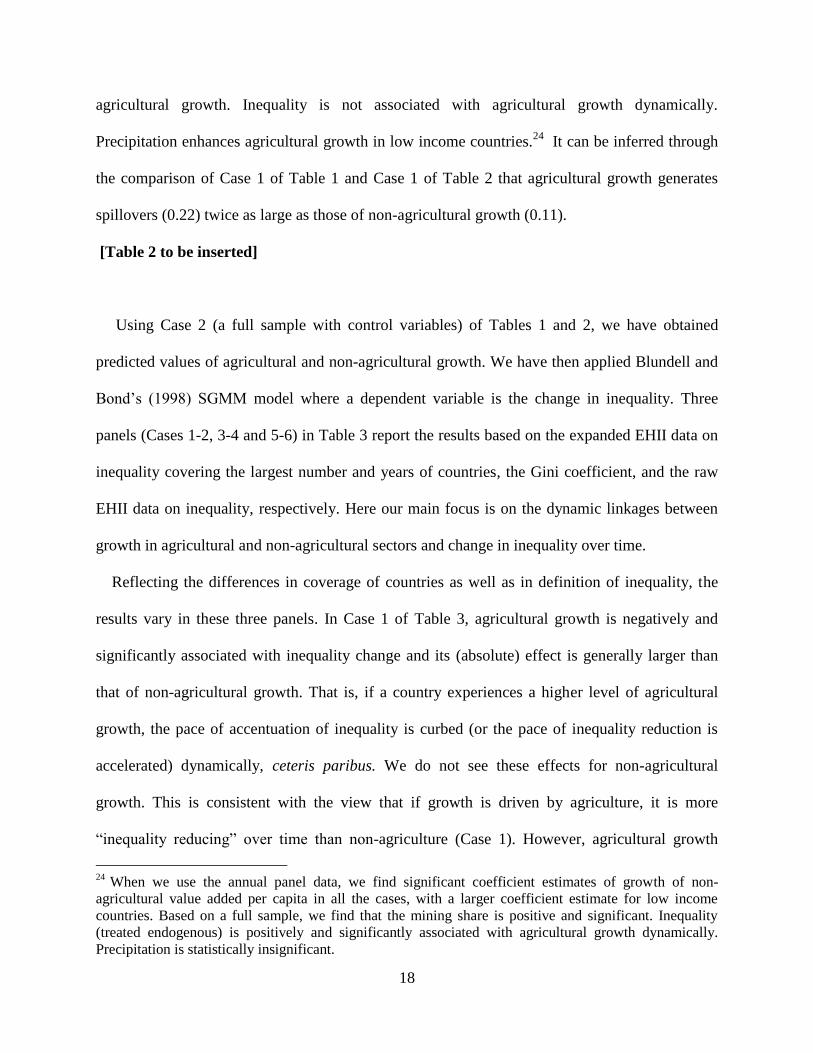
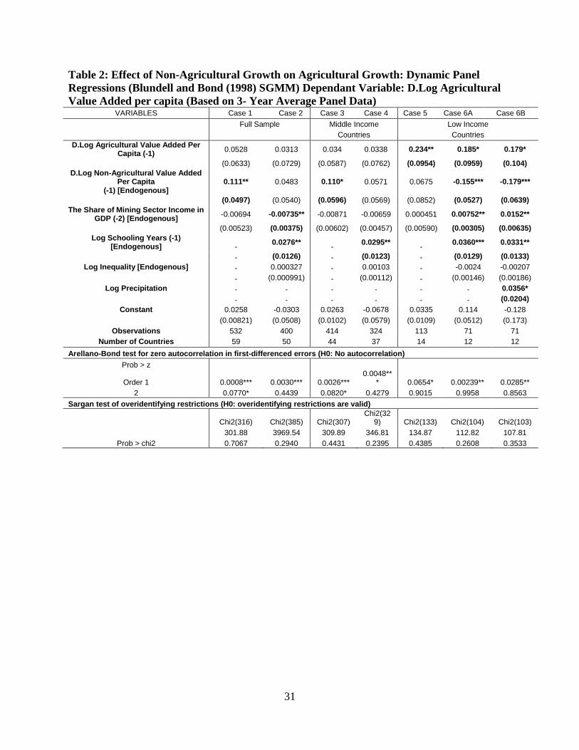
In Table 2 we estimate the effect of non-agricultural growth on agricultural growth. Table 2

reports positive and significant coefficient estimates of lagged growth in non-agricultural value

added on growth of agricultural value added in Case 1 based on a full sample and Case 3 for

middle income countries.23

However, it is negative and significant in Cases 6A and 6B for low

income countries. A lagged dependent variable is positive with significant estimates observed

only for low income countries. The share of mining sector is negative for the full sample, with

the coefficient estimate significant only in Case 2. This result could be related to the large

literature on the Dutch Disease where, for instance, Nigerian cocoa farmers uprooted cacao

plants following the petroleum boom in the 1970s (Roemer, 1985). It is, however, positive and

significant for low income countries (in Cases 6A and 6B) and negative and insignificant for

middle income countries. The positive effect could reflect positive externalities from the mining

sector to agricultural sector (e.g. better roads, power supply), while the negative effect could be

due to displacement of the agricultural sector by the mining sector. Human capital enhances

21

A possible reason is that a higher (initial) inequality in a poor country might enable wealthier people to

invest in high-return and high-risk activities and increase the overall efficiency of the non-farm sector. If

the country’s wealth is more equally distributed with a majority under the poverty line, such efficient

investment may not be easy. Overall, at the earlier stage of development, rural society is homogeneous

with less degree of inequality, but inequality will expand as the country grows at certain threshold

(Kuznets, 1955, 1963). 22

The choice of Case 2 is guided by the specification test results showing that there is no second order

serial correlation and that over-identifying restrictions are valid. 23

These results will be unchanged if we run the same regression using the sample before 2005.

18

agricultural growth. Inequality is not associated with agricultural growth dynamically.

Precipitation enhances agricultural growth in low income countries.24

It can be inferred through

the comparison of Case 1 of Table 1 and Case 1 of Table 2 that agricultural growth generates

spillovers (0.22) twice as large as those of non-agricultural growth (0.11).

[Table 2 to be inserted]

Using Case 2 (a full sample with control variables) of Tables 1 and 2, we have obtained

predicted values of agricultural and non-agricultural growth. We have then applied Blundell and

Bond’s (1998) SGMM model where a dependent variable is the change in inequality. Three

panels (Cases 1-2, 3-4 and 5-6) in Table 3 report the results based on the expanded EHII data on

inequality covering the largest number and years of countries, the Gini coefficient, and the raw

EHII data on inequality, respectively. Here our main focus is on the dynamic linkages between

growth in agricultural and non-agricultural sectors and change in inequality over time.

Reflecting the differences in coverage of countries as well as in definition of inequality, the

results vary in these three panels. In Case 1 of Table 3, agricultural growth is negatively and

significantly associated with inequality change and its (absolute) effect is generally larger than

that of non-agricultural growth. That is, if a country experiences a higher level of agricultural

growth, the pace of accentuation of inequality is curbed (or the pace of inequality reduction is

accelerated) dynamically, ceteris paribus. We do not see these effects for non-agricultural

growth. This is consistent with the view that if growth is driven by agriculture, it is more

“inequality reducing” over time than non-agriculture (Case 1). However, agricultural growth

24

When we use the annual panel data, we find significant coefficient estimates of growth of non-

agricultural value added per capita in all the cases, with a larger coefficient estimate for low income

countries. Based on a full sample, we find that the mining share is positive and significant. Inequality

(treated endogenous) is positively and significantly associated with agricultural growth dynamically.

Precipitation is statistically insignificant.

19

ceases to be statistically significant in Case 2 with a few control variables (education and

political stability) and non-agricultural growth becomes statistically significant.25

[Table 3 to be inserted]

In Cases 3 and 4 of Table 3, neither agricultural nor non-agricultural growth is significant in

which the change in the Gini coefficient is a dependent variable. We observe a strong persistence

in the change in the Gini coefficient in Cases 3 and 4. So in these cases agricultural and non-

agricultural growth do not affect inequality changes. In Cases 5 and 6, the raw EHII data are

used for the measure of inequality and the dynamic model is applied. In these cases agricultural

growth is not statistically significant, while non-agricultural growth is negative and significant in

Case 6 where schooling and political stability are added as control variables. This is consistent

with the inequality reducing effect of non-agricultural growth which we have found in Case 2.

While the results vary depending on the specifications, agricultural growth has an inequality-

reducing effect in the case without controlling for schooling years and political stability. Once

we control for these variables, non-agricultural sector has some inequality-reducing effect.

In Table 4 we use the annual panel data to estimate the effects of agricultural growth and non-

agricultural growth on inequality. Three measures of inequality are used as a dependent variable

in three panels - the first difference in inequality based on the expanded EHII data (Cases 1-4),

the Gini coefficient (Cases 5-6), and inequality based on the raw EHII data (Cases 7-8). In cases

where the expanded EHID data are used, we have applied both Blundell and Bond’s (1998)

25

The difference between Case 1 and Case 2 of Table 3 (i.e. agricultural growth becomes statistically

non-significant, while non-agricultural growth becomes significant in Case 2) appears to be due to the fact

that schooling and governance are more highly and positively correlated with agricultural growth (with

the coefficient of correlation of 0.625 and 0.404, respectively) than with non-agricultural growth (0.157

and 0.046, respectively).

20

SGMM model and MG estimator (Pesaran and Smith, 1995) and CCEMG estimator (Pesaran,

2006) to take account of the cross-country dependence of error terms. On the contrary, only fixed

effects model is applied for Cases 5 and 6 in which the change in the Gini is estimated as this is a

highly unbalanced panel. In Cases 7 and 8 with the raw EHII data of inequality, only SGMM

model is applied.

When the expanded EHII data on inequality are used, we find that agricultural growth tends

to reduce accentuation of inequality, as suggested by the negative and significant coefficients of

(predicted) agricultural growth in Cases 1, 3, 5 and 6. The range of coefficient estimates (-3.27 to

-3.97) in Cases 1-5 is much smaller than that based on three-year panel data, reflecting the

difference in the data structure. Using a semi-log specification, the coefficient estimate of

agricultural (or non-agricultural) growth captures how many percentage points will be changed

in response to a one percentage point increase in agricultural (or non-agricultural) growth in a

year in Table 4, while the same calculation applies to the three year period in Table 3. If

agricultural growth increases by 1%, the change in inequality decreases by 3.3% on average,

ceteris paribus (Case 1 of Table 4). Recalling the fact that we have the (time-series) average in

agricultural growth, the estimate in Case 6 has changed to -6.0. Indeed, the effect of non-

agricultural sector growth in reducing the inequality change is much larger (with the estimates

ranging from -14.4 to -9.8). This is consistent with Bourguignon and Morrisson who show that

an increase in relative labour productivity (non-agriculture/agriculture) tends to increase

inequality (or ratio of share of top 20% to bottom 60%).

[Table 4 to be inserted]

21

However, when we estimate the first difference in Gini coefficient by fixed-effects model

(Cases 5 and 6), neither agricultural or non-agricultural growth is statistically significant. In

Cases 7 and 8 where the raw EHII data on inequality are used, we do not find any negative and

significant coefficient estimate as we did in Cases 1-2. In Cases 7 and 8 with the dynamic model,

signs of coefficient estimates of agricultural and non-agricultural growth are negative, but

statistically insignificant. 26

While the results vary depending on the specifications, if we rely on

the results based on the expanded EHII data on inequality, we can conclude that both agricultural

and non-agricultural growth accelerate inequality reduction over time.

Given the variation of signs of agricultural and non-agricultural growth terms in Tables 3 and

4, it is difficult to derive a single conclusion about the effects of sectoral growth on inequality.

However, if we rely on the results of the dynamic panel model in Table 3 based on three years

average data where the model adjusts for short-term fluctuations and measurement errors as well

as takes account of the endogeneity of sectoral growth, we can conclude that agricultural

agricultural growth has some inequality reducing effect (Case 1 of Table 3). We have also found

that non-agricultural growth accelerates inequality reduction once we control for schooling years

and political stability.

Using the country-level coefficient estimates based on the CCEMG model based on the

expanded EHII data on inequality (Case 4, Table 4), we have checked which factors are

associated with the country-level estimates of the effect of agricultural or non-agricultural

26

It is conjectured that instability of agricultural growth, which is, for instance, affected by weather

conditions – would make the impact of agricultural growth on inequality weaker in the short run because

a part of income fluctuations may be well insured by both the rich and the poor (e.g. Townsend, 1994). In

the medium run, this attenuating effect may be less relevant and the inequality reducing effect of each

sector is more accurately estimated. It is noted that the coefficient of variation of annual growth (there-

year average growth) is 22.2 (8.5) for agricultural sector and 5.0 (3.0) for non-agricultural sector. Our

main conclusion is thus derived by (follows from) the results of three-year average panel data.

22

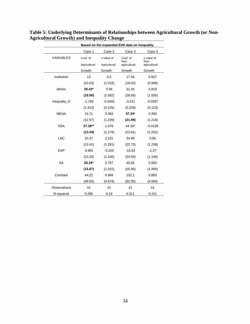
growth on inequality change by running a simple OLS (Ordinary Least Squares) (Table 5).

Appendix 3 reports the country-level coefficient estimates and z values on the CCEMG model.

[Table 5 to be inserted]

In Cases 1-4 of Table 5 where the expanded data on inequality are used, we find several

statistically significant coefficient estimates. First, if a country is more ethnically fractionalised,27

it tends to have a higher (i.e., more positive or less negative) value in the coefficient indicating

the effect of agricultural growth on inequality changes. This implies that the role of agriculture in

reducing accentuation of inequality is likely to be undermined by ethnic fractionalisation which

tends to make economic inequality more persistent. This is understandable because if the country

consists of different ethnic groups, typically with a few ethnic minority groups which may be

excluded from development process of agriculture (e.g. mechanisation), agricultural growth may

have little impact on inequality over time, other factors being unchanged. Second, in Case 1,

there is some regional diversity in the linkages between agricultural or non-agricultural growth

and inequality change. For instance, countries in Sub-Saharan Africa tend to experience slower

changes in improvement in equality as a result of growth in both agricultural and non-

agricultural sectors. South Asian countries also tend to have slow changes as a result of

agricultural growth. Countries in Middle East and North Africa have tended to experience slower

changes in improvement in equality as a result of growth in non-agricultural sectors. This could

27

The index of ethnic fractionalisation is based on Alesina et al. (2003) and indicates the degree of

fractionalisation of ethnic groups where the definition of ethnicity involves a combination of racial and

linguistic characteristics. A high value implies that the country consists of different ethnic groups, while a

low value indicates homogeneous ethnic composition.

23

be due to the higher share of resource dependency (e.g. oil) in many countries in these regions

where corruption may perpetuate inequality (e.g. Gupta, et al., 2002).

Inequality index used in the analysis for Tables 3 and 4 reasonably captures overall economic

inequality of a country (Galbraith and Kum, 2005). However, given the aforementioned

limitation of our inequality measure, it would be also useful to see how agricultural growth or

non-agricultural growth affects poverty, which is defined by the poverty headcount ratio or the

poverty gap, following Christiaensen et al. (2011).28

Table 6 reports the results on the effect of

agricultural or non-agricultural growth on poverty headcount ratio or poverty gap - for a full

sample of countries (Panel A), middle income countries (Panel B) and low income countries

(Panel C). Following Christiaensen et al. (2011), we apply the country-fixed effects model29

and

use only predicted values of agricultural or non-agricultural growth (based on Case 2 in Table 1

and Case 2 in Table 2) without adding further control variables.30

[Table 6 to be inserted]

Table 6 shows that agricultural growth has a stronger and significant effect in reducing both

poverty headcount ratio and poverty gap regardless of whether the US$1.25 a day poverty line or

the US 2.00 a day poverty line is adopted, while there is no statistically significant effect of non-

agricultural growth on either poverty headcount or poverty gap. The pattern of the results is

broadly unchanged if we restrict the sample only to middle income countries where agricultural

28

If we generate the first differences in poverty, the number of observations will be reduced significantly

due to missing observations. So we use these poverty indices in levels, rather than first differences. 29

The Hausman test results favour fixed effects model over random effects model. 30

Adding further control variables is difficult in the regressions in Table 6 as we use a restricted sample

with disaggregated sectoral data available in this section. Nor did Christiaensen et al. (2011) in their

poverty regressions. It should also be noted that use of other cases (Case 1 of Tables 1 and 2) will not

change the results significantly.

24

growth is found to reduce poverty regardless of which definition is used. On the other hand, in

the case of low income countries, with the caveat that this is based on a small number of

observations, we find a statistically significant coefficient estimate of agricultural growth only in

Case 10 on poverty gap based on US$1.25 line. Poverty reducing effects of agricultural growth

are weaker in terms of their magnitude for low income countries than for middle income

countries. Non-agricultural growth is negative and statistically insignificant for both middle and

low income countries, with the coefficient estimates larger for the latter. We confirm that

agricultural growth has a stronger poverty-reducing effect than non-agricultural growth. This is

consistent with Table 6 of Christiaensen et al. (2011, p.248) which shows a stronger poverty

reducing effect at the US$1 threshold, but not Table 7 (p.249) in which while agricultural and

non-agricultural growth significantly reduce US$2 poverty, the effect of non-farm sector growth

becomes more prominent as its effect is larger than that of agricultural growth in 4 out of 8 cases

and statistically significant in all cases. A similar pattern, however, is found in Case 11 where

non-agricultural growth is statistically significant, while agricultural growth is not.

6. Concluding Observations

Drawing upon cross-country panel data for developing countries, the present study sheds new

empirical light on the dynamic and long-term linkages among agricultural growth, inequality and

poverty in developing countries. Using econometric models, we have analysed in detail whether

agricultural growth impacts inequality and poverty after taking account of the dynamic linkages

between the agricultural and the non-agricultural sectors over time. To understand the relative

role of agricultural sector, we have compared the effect of agricultural growth and that of non-

agricultural growth on inequality and poverty. The analyses draw upon both dynamic and static

25

panel models using three-year averages covering the period 1969-2010. This is supplemented by

the annual panel data for the same period. The main findings are summarised below from a

policy perspective.

First, we generally observe strong growth linkages between agricultural and non-agricultural

sectors for all developing countries (full sample) and middle income countries. Lagged

agricultural growth - which is treated as an endogenous variable in the model - tends to promote

non-agricultural growth, while lagged (endogenous) non-agricultural growth also tends to

enhance agricultural growth. We, however, have found that agricultural growth generates

spillovers twice as large as those of non-agricultural growth.

Second, in the case where the expanded EHII data are used, agricultural growth is found to

reduce accentuation of inequality, or accelerate inequality reduction. While such inequality

reducing effects of agricultural growth are found in the short-run based on the annual panel, non-

agricultural growth tends to reduce inequality faster in the short run. In this case, the degree of

ethnic fractionalisation is key to explaining the magnitude of negative linkages between

agricultural/non-agricultural growth and inequality changes in the short term. That is, the role of

agricultural sector reducing accentuation of inequality is likely to be undermined by ethnic

fractionalisation which tends to make inequality more persistent. However, once we use the Gini

coefficient or the inequality based on raw EHII data - which reflects wage inequality in

manufacturing sector -, these relationships are no longer observed. There is no clear relationship

between sectoral growth and changes in Gini coefficient in either the short or the medium term.

When we use raw EHII data of inequality, we observe an inequality reducing effect of non-

agricultural growth in the medium run.

26

Third, agricultural growth reduces poverty - both headcount ratios and poverty gaps - in both

middle income and low income countries. Such poverty reducing effects are not clearly observed

for non-agricultural growth. Our results thus reinforce the role of overall agricultural sector in

promoting overall economic growth and reducing poverty.

The World Bank recently strongly endorsed the case for promoting rural-urban migration and

concomitant shift of resources towards efficient urbanisation, as reported in Global Monitoring

Report 2013, Monitoring the MDGs (World Bank, 2013). However, this claim has been robustly

rejected by our analysis that reinforces the case for revival of agriculture. Our conclusion - based

on sophisticated econometric modelling and updated data - is consistent with the World Bank’s

earlier position supporting the role of agricultural sector in reducing poverty (e.g. World

Development Report 2008 (World Bank, 2007))31

.

Agricultural sector continues to have strong linkages with the non-agricultural sector and has

substantial potential for reducing inequality and poverty. More seriously, if our analysis has any

validity, the lop-sided shift of emphasis to urbanisation rests on not just shaky empirical

foundations but could mislead policy makers and donors. Those left behind in rural areas -

especially the poor - deserve better and more resources to augment labour productivity in

agriculture to speed up overall growth and eliminate worst forms of deprivation in the post-2015

scenario.

References

Acemoglu, D., & Robinson, J. A. (2002). The Political Economy of the Kuznets Curve. Review

of Development Economics, 6(2), 183–203.

31

World Bank (2007) concludes that ‘(I)n the 21st century, agriculture continues to be a fundamental

instrument for sustainable development and poverty reduction’ (p.1).

27

Arellano, M., & Bond, S. (1991). Some tests of specification for panel data: Monte Carlo

evidence and an application to employment equations. Review of Economic Studies, 58, 277-

297.

Alesina, A., Devleeschauwer, A., Easterly, W., Kurlat, S., & Wacziarg, R. (2003).

Fractionalization. Journal of Economic Growth, 8, 155-194.

Arellano, M., & Bover, O. (1995). Another look at the instrumental variable estimation of error-

components models. Journal of Econometrics, 68, 29-51.

Baltagi, B.H. (2005). Econometric Analysis of Panel Data. Third Edition. Chichester: John

Wiley & Sons Ltd.

Barro, R.J. (2000). Inequality and Growth in a Panel of Countries. Journal of Economic Growth,

5, 5–32.

Barro, R.J., & Lee, J. (2010). A New Data Set of Educational Attainment in the World, 1950–

2010. NBER Working Paper No. 15902. Cambridge MA: NBER.

Bourguignon, F., & Morrisson, C. (1998). Inequality and development: the role of dualism.

Journal of Development Economics. 57. 233-257.

Blundell, R., & Bond, S. (1998). Initial conditions and moment restrictions in dynamic panel

data models. Journal of Econometrics, 87, 115-143. A.

Christiaensen, L., Demery, L., & Kuhl, J. (2011). The (evolving) role of agriculture in poverty

reduction: An empirical perspective. Journal of Development Economics, 96(2), 239-254.

Collier, P. (2008). The Bottom Billion: Why the Poorest Countries are Failing and What Can Be

Done About It, Oxford, Oxford University Press.

Collier, P., & Dercon, S. (2014). African Agriculture in 50 years: Smallholders in a Rapidly

Changing World?. World Development, 63, 92-101.

28

de Janvry, A., & Sadoulet, E. (2010). Agricultural Growth and Poverty Reduction: Additional

Evidence. The World Bank Research Observer, 25(1), 1 – 20.

Deininger, K., & Squire, L. (1996). A New Data Set Measuring Income Inequality. World Bank

Economic Review, 10, 565–591.

Doyle, M. W., & Stiglitz, J.E. (2014). Eliminating Extreme Inequality: A Sustainable

Development Goal, 2015–2030, Ethics & International Affairs, 28(1), 5-13.

Galbraith, J. K., & Kum, H. (2005) Estimating the Inequality of Household Incomes: A

Statistical Approach to the Creation of a Dense and Consistent Global Data Set, Review of

Income and Wealth, 51(1), 115–143.

Gupta, S., Davoodi, H., & Alonso-Terme, R. (2002). Does corruption affect income inequality

Economics of Governance, 3(1), 23-45.

Haggblade, S., & Hazell, P. (1989). Agricultural technology and farm-nonfarm growth linkages.

Agricultural Economics, 3(4), 345–364.

Haggblade, S., Hazell, P. & Dorosh, P. (2007). Sectoral growth linkages between agriculture and

the rural nonfarm economy. In Haggblade, S., Hazell, P., & Reardon, T. (eds), Transforming

the Rural Nonfarm Economy—Opportunities and Threats in the Developing World.

Baltimore, Johns Hopkins University Press.

Hayakawa, K. (2007). Small sample bias properties of the system GMM estimator in dynamic

panel data models. Economics Letters, 95, 32–38.

Herzer, D, & Vollmer, S. (2012). Inequality and growth: evidence from panel cointegration.

Journal of Economic Inequality, 10, 489–503.

Kuznets, S. (1955). Economic growth and income inequality. American Economic Review, 45, 1-

28.

29

Kuznets, S. (1963). Quantitative aspects of the economic growth of nations. Economic

Development and Cultural Change, 12, 1-80.

Pesaran, M.H. (2006). Estimation and inference in large heterogeneous panels with a multifactor

error structure. Econometrica, 74, 967-1012.

Pesaran, M.H., & Smith, R. (1995). Estimating long-run relationships from dynamic

heterogeneous panels. Journal of Econometrics, 68, 79-113.

Roemer, M. 1985. Dutch disease in developiong countries: swallowing bitter medicine. In

Lundahl (ed), The Primary Sector in Economic Development, pp.201-226.

Thapa, G., & Gaiha, R. (2014). ‘Smallholder Farming in Asia and the Pacific: Challenges and

Opportunities’. In Hazell, P., & Rahman, A. (eds) New Directions in Smallholder Agriculture.

Oxford and Rome, Oxford University Press & International Fund for Agricultural

Development.

Townsend, R. M. (1994). Risk and Insurance in Village India. Econometrica, 62(3), 539-591.

United Nations (2013). Inequality Matters, Report on the World Social Situation 2013. New

York, United Nations, http://www.un.org/en/development/desa/publications/world-social-

situation-2013.html.

Windmeijer, F. (2005). A finite sample correction for the variance of linear efficient twostep

GMM estimators. Journal of Econometrics.126, 25–51.

World Bank (2007). World Development Report 2008: Agriculture for Development,

Washington DC, World Bank.

World Bank (2013). Global Monitoring Report 2013: Monitoring the MDGs, Washington DC,

World Bank.

World Bank (2014). World Development Indicators, Washington DC, World Bank.

30

Table 1: Effect of Agricultural Growth on Non-Agricultural Growth Dynamic Panel

Regressions (Blundell and Bond (1998) SGMM): Dependant Variable: D.Log Non

Agricultural Value Added per capita (based on 3- Year Average Panel Data) VARIABLES Case 1 Case 2 Case 3 Case 4 Case 5 Case 6

Full Sample Middle Income Low Income

Countries Countries

D.Log Non Agricultural Value Added per capita (-1)

0.261*** 0.309*** 0.223** 0.211** 0.502*** 0.504***

(0.0988) (0.0535) (0.105) (0.102) (0.129) (0.129)

D.Log Agricultural Value Added per capita [Endogenous]

0.224*** 0.143* 0.122 0.171** 0.0702 0.088

(0.0865) (0.0761) (0.0761) (0.0840) (0.141) (0.153)

The Share of Mining Sector Income in GDP (-2) [Endogenous]

0.000488 0.000773 -0.00398 -0.00254 0.000118 -0.00172

(0.00781) (0.00586) (0.00926) (0.00738) (0.00593) (0.00542)

D.Log Investment [Endogenous] - 0.214*** - - - -

- (0.0310) - - - -

Log Schooling Years (-1) [Endogenous] - 0.0205* - - - -

- (0.0117) - - - -

Log Inequality [Endogenous] - 0.00186* - - - -

- (0.000971) - - - -

D.Log Agricultural Value Added per capita * SSA Dummy [Endogenous] - - -

-0.0719 -

0.0201

- - - (0.121) - (0.146)

Constant 0.0443 -0.0686 0.0455 0.0436 0.0540 0.0534

(0.0128) (0.0484) (0.0155) (0.0150) (0.0194) (0.0194)

Observations 532 400 414 414 113 113

Number of Countries 59 50 44 44 14 14

Arellano-Bond test for zero autocorrelation in first-differenced errors (H0: No autocorrelation)

Prob > z

Order 1 0.0030*** 0.0032*** 0.0098*** 0.0094*** 0.1308 0.1266

2 0.1916 0.2548 0.1894 0.1853 0.2813 0.2379

Sargan test of overidentifying restrictions (H0: overidentifying restrictions are valid)

Chi2(316) Chi2(399) Chi2(307) Chi2(366) Chi2(133) Chi2(143)

375.66 414.60 392.864 457.17 170.30 183.08

Prob > chi2 0.00118** 0.2848 0.0007*** 0.0008*** 0.0161** 0.0133**

31

Table 2: Effect of Non-Agricultural Growth on Agricultural Growth: Dynamic Panel

Regressions (Blundell and Bond (1998) SGMM) Dependant Variable: D.Log Agricultural

Value Added per capita (Based on 3- Year Average Panel Data) VARIABLES Case 1 Case 2 Case 3 Case 4 Case 5 Case 6A Case 6B

Full Sample Middle Income Low Income

Countries Countries

D.Log Agricultural Value Added Per Capita (-1)

0.0528 0.0313 0.034 0.0338 0.234** 0.185* 0.179*

(0.0633) (0.0729) (0.0587) (0.0762) (0.0954) (0.0959) (0.104)

D.Log Non-Agricultural Value Added Per Capita

(-1) [Endogenous] 0.111** 0.0483 0.110* 0.0571 0.0675 -0.155*** -0.179***

(0.0497) (0.0540) (0.0596) (0.0569) (0.0852) (0.0527) (0.0639)

The Share of Mining Sector Income in GDP (-2) [Endogenous]

-0.00694 -0.00735** -0.00871 -0.00659 0.000451 0.00752** 0.0152**

(0.00523) (0.00375) (0.00602) (0.00457) (0.00590) (0.00305) (0.00635)

Log Schooling Years (-1) [Endogenous] -

0.0276** -

0.0295** -

0.0360*** 0.0331**

- (0.0126) - (0.0123) - (0.0129) (0.0133)

Log Inequality [Endogenous] - 0.000327 - 0.00103 - -0.0024 -0.00207

- (0.000991) - (0.00112) - (0.00146) (0.00186)

Log Precipitation - - - - - - 0.0356*

- - - - - - (0.0204)

Constant 0.0258 -0.0303 0.0263 -0.0678 0.0335 0.114 -0.128

(0.00821) (0.0508) (0.0102) (0.0579) (0.0109) (0.0512) (0.173)

Observations 532 400 414 324 113 71 71

Number of Countries 59 50 44 37 14 12 12

Arellano-Bond test for zero autocorrelation in first-differenced errors (H0: No autocorrelation)

Prob > z

Order 1 0.0008*** 0.0030*** 0.0026*** 0.0048**

* 0.0654* 0.00239** 0.0285**

2 0.0770* 0.4439 0.0820* 0.4279 0.9015 0.9958 0.8563

Sargan test of overidentifying restrictions (H0: overidentifying restrictions are valid)

Chi2(316) Chi2(385) Chi2(307) Chi2(32

9) Chi2(133) Chi2(104) Chi2(103)

301.88 3969.54 309.89 346.81 134.87 112.82 107.81

Prob > chi2 0.7067 0.2940 0.4431 0.2395 0.4385 0.2608 0.3533

32

Table 3: Effect of Predicted Agricultural/Non-Agricultural Growth on Inequality Change:

Dependent Variable: D.Inequality: (based on 3- year average panel)

Based on the expanded EHII data

on inequality Based on Gini

Based on the raw EHII data on

inequality

Blundell and Bond (1998) SGMM (dynamic panel)

Case 1 Case 2 Case 3 Case 4 Case 5 Case 6

VARIABLES Full Sample Full Sample Full Sample

D.Inequality (-1) -0.0527 -0.150** 0.820*** 0.643*** 0.786*** 0.770***

(0.0666) (0.0617) (0.0706) (0.107) (0.0928) (0.0579)

Log Schooling Years [Endogenous] - -0.488 - -0.745 - -0.475**

- (0.307) - (0.577) - (0.196)

Political Stability [Endogenous] - -0.182 - 0.275 - -0.199

- (0.75) - (0.868) - (0.736)

D.Log Agricultural Value Added per capita [Predicted]

-29.72* -15.22 -36.51 45.32 -2.254 20.79

(17.57) (29.19) (34.47) (48.15) (18.60) (21.10)

D.Log Non-Agricultural Value Added per capita [Predicted]

-4.091 -9.945** 4.254 -7.677 -4.556 -9.546***

(3.64) (4.493) (7.977) (7.807) (3.707) (2.171)

Constant 1.237 4.925 8.34 19.33 10.25** 13.86***

(0.524) (1.875) (2.887) (6.484) (4.324) (3.174)

Observations 383 206 167 129 278 129

Number of Countries 47 43 42 39 42 38

R-squared

Arellano-Bond test for zero autocorrelation in first-differenced errors (H0: No autocorrelation)

Prob > z

Order 1 0.0003*** 0.0160** 0.0022*** 0.0064*** 0.0719* 0.0218**

2 0.0629* 0.22 0.911 0.6842 0.2411 0.4516

Sargan test of overidentifying restrictions (H0: overidentifying restrictions are valid)

Chi2(114) Chi2(127) Chi2(46) Chi2(79) Chi2(107) Chi2(85)

152.22 136.99 47.47 76.64 163.29*** 94.20

Prob > chi2 0.0097 0.2569 0.4172 0.5543 0.0004 0.2319

33

Table 4: Effect of Predicted Agricultural/Non-Agricultural Growth on Inequality Change (Based on Annual panel)

Based on the expanded EHII data on inequality Based on Gini Coefficient Based on the raw EHII data

on inequality VARIABLES Case 1 Case 2 Case 3 Case 4 Case 5 Case 6 Case 7 Case 8

Blundell and Bond (1998)

MG Estimator Pesaran &

Smith

Fixed Effects Model Blundell and Bond (1998)

SGMM (Dynamic Panel (Robust Estimators) SGMM (Dynamic Panel D.Inequality (-1) -0.0593* *

1 -0.0772 - - - - 0.743***

1 0.676***

(0.0351) (0.108) - - - - (0.107) (0.0794) Log Schooling Years

[Endogenous] - -0.113

- - - - -0.280***

- (0.114) - - - - (0.0949)

Political Stability - 0.0171 - - - - -0.567**

- (0.293) - - - - (0.259)

D.Log Agricultural Value Added per capita [Predicted]

*2

-3.270* -3.166 -3.973** -6.030** -0.144 -0.854 -0.511 -1.897

(1.730) (3.005) (1.992) (2.646) (5.042) (0.590) (1.695) (1.445) D.Log Non-Agricultural Value Added per capita [Predicted]

*2

-11.47*** -14.41** -10.04** -11.14** 0.976 0.423 -0.0422 -5.023

(4.354) (5.985) (4.182) (4.695) (18.16) (0.780) (5.855) (3.904) Trend - - -0.00423 -0.0013 - 3.685 - -

- - (0.00724) (0.00839) - (3.265) - -

D.Log Inequality_avg - - - 0.424** - 15.84 - -

- - - (0.175) - (15.04) - -

D.Log Agricultural Value Added per capita [Predicted]_avg - - -

7.117 - - - -

- - - (6.309) - - - -

D.Log Non-Agricultural Value Added per capita [Predicted]_avg - - -

4.449 - - - -

- - - (9.730) - - - -

Constant 0.360 1.328 0.613 0.14 - - 11.54 16.71***

(0.113) (0.853) (0.280) (0.342) - - (4.668) (3.654) Observations 849 360 927 927 338 216 791 301

Number of Countries 45 40 45 45 48 41 42 36 R-squared

41.72 48.33 Arellano-Bond test for zero autocorrelation in first-differenced errors (H0: No autocorrelation)

Prob > z Order 1 0.0005*** 0.0180*** - - - - 0.0017*** 0.0127***

2 0.8820 0.5317 - - - - 0.2065 0.4276 Sargan test of overidentifying restrictions (H0: overidentifying restrictions are valid)

Chi2(764) Chi2(331) Chi2(713) Chi2(271) 863.50 334.89 - - - - 984.460 330.00

Prob > chi2 0.0070*** 0.4376 - - - - 0.0000*** 0.0028 Notes: 1. Robust standard errors in parentheses. *** p<0.01, ** p<0.05, * p<0.1. Statistically significant coefficient estimates are shown in bold. 2. Agricultural growth and non-agricultural growth are estimated by the Blundell and Bond (1998) SGMM model using annual panel data where the specification is same as Case 2 (with control variables) of Tables 1 and 2.

34

Table 5: Underlying Determinants of Relationships between Agricultural Growth (or Non-

Agricultural Growth) and Inequality Change

Based on the expanded EHII data on inequality

Case 1 Case 2 Case 3 Case 4

VARIABLES Coef. of z value of Coef. of z value of

Agricultural Agricultural

Non-agricultural

Non-agricultural

Growth Growth Growth Growth

Institution 13 0.5 17.06 0.607

(10.63) (1.015) (18.02) (0.998)

ethinic 28.43* 0.58 31.45 0.818

(16.56) (1.582) (28.08) (1.555)

inequality_D -1.769 -0.0491 -3.411 -0.0397

(1.313) (0.125) (2.226) (0.123)

MENA 15.71 0.383 37.34* 0.393

(12.97) (1.239) (21.99) (1.218)

SSA 27.28** 1.079 44.30* -0.0139

(13.34) (1.274) (22.61) (1.252)

LAC 20.37 2.131 34.89 0.85

(13.41) (1.281) (22.73) (1.259)

EAP -0.891 -0.203 -15.63 -1.37

(12.20) (1.166) (20.69) (1.146)

SA 28.18* 0.797 40.65 0.563

(15.87) (1.515) (26.90) (1.490)

Constant 44.22 0.966 102.1 0.883

(48.93) (4.674) (82.95) (4.594)

Observations 41 41 41 41

R-squared 0.286 0.19 0.311 0.151

35

Table 6: Effect of Predicted Agricultural/Non-Agricultural Growth on Poverty: Based on 3

-year panel, country fixed effects estimation

Panel A: Full Sample VARIABLES Case 1 Case 2 Case 3 Case 4

Poverty Head

Count Poverty Gap

Poverty Head Count

Poverty Gap

US$1.25 US$1.25 US$2.00 US$2.00

Full Sample Full Sample

D.Log Agricultural Value Added per capita [Predicted] -28.97*** -25.77*** -19.86*** -23.60***

(10.60) (7.529) (7.298) (6.448)

D.Log Non-Agricultural Value Added per capita [Predicted]

-1.151 -0.638 -0.578 -1.616

(1.841) (1.360) (1.350) (1.454)

Constant 2.372 1.223 3.189 2.294

(0.283) (0.186) (0.195) (0.185)

Observations 234 227 234 232

R-squared 0.165 0.182 0.13 0.234

Number of Countries 45 45 45 45

Panel B: Middle Income Countries VARIABLES Case 5 Case 6 Case 7 Case 8

Poverty Head

Count Poverty Gap

Poverty Head Count

Poverty Gap

US$1.25 US$1.25 US$2.00 US$2.00

Middle Income Middle Income

Countries Countries

D.Log Agricultural Value Added per capita [Predicted] -30.95** -25.36*** -21.81** -24.98***

(12.40) (8.398) (8.567) (7.446)

D.Log Non-Agricultural Value Added per capita [Predicted] -0.822 -0.318 -0.339 -1.449

(2.008) (1.459) (1.469) (1.572)

Constant 2.031 0.848 2.960 2.008

(0.325) (0.206) (0.225) (0.209)

Observations 193 186 193 191

R-squared 0.156 0.161 0.126 0.226

Number of Countries 35 35 35 35

Panel C: Low Income Countries VARIABLES Case 9 Case 10 Case 11 Case 12

Poverty Head

Count Poverty Gap

Poverty Head Count

Poverty Gap

US$1.25 US$1.25 US$2.00 US$2.00

Low Income Low Income

Countries Countries

D.Log Agricultural Value Added per capita [Predicted] -19.59 -30.94* -10.36 -18.96

(13.27) (16.13) (8.842) (11.81)

D.Log Non-Agricultural Value Added per capita [Predicted] -3.611 -3.588 -2.071 -2.343

(2.203) (2.990) (1.124) (1.585)

Constant 4.354 3.401 4.607 3.950

(0.263) (0.320) (0.190) (0.253)

Observations 39 39 39 39

R-squared 0.472 0.448 0.453 0.466

Number of Countries 9 9 9 9

Notes: Robust standard errors in parentheses. *** p<0.01, ** p<0.05, * p<0.1. Statistically significant coefficient estimates are shown in bold.

36

Appendix 1: A List of countries included in the base case (Case 2, Table 1 and 2)

Albania, Algeria, Argentina, Bangladesh, Bolivia, Brazil, Bulgaria, Cameroon, Chile, China,

Colombia, Congo, Rep., Cote d'Ivoire, Ecuador, Egypt, Arab Rep., Gabon, Guatemala, Hungary,

India, Indonesia, Iran, Islamic Rep., Jordan, Kazakhstan, Kyrgyz Republic, Lithuania, Malaysia,

Mauritania, Mexico, Moldova, Morocco, Pakistan, Peru, Philippines, Poland, Romania, Russian

Federation, Senegal, Serbia, Slovak Republic, Slovenia, South Africa, Sudan, Tajikistan,

Thailand, Tunisia, Ukraine, Vietnam, Yemen, Rep.

Appendix 2: Descriptive Statistics (3 year average)

Variable

Mean Std. Dev. Min Max Observations

Log agricultural value overall 4.522191 3.528402 -14.31253 6.508571 N = 400

Added per capita between

2.832785 -14.25602 6.205418 n = 50

within

0.1558084 3.927754 5.064494 T = 8

log non agricultural overall 6.396096 3.972115 -14.26882 9.725732 N = 400

value added per capita between

3.261406 -14.00379 9.543673 n = 50

within

0.3189024 4.79499 7.975028 T = 8

log share of mining overall 0.6489725 2.200495 -7.736457 4.60517 N = 393

sector between

2.470386 -7.341874 4.60517 n = 49

within

0.7346914 -2.297781 6.016172 T = 8.02041

log average schooling overall 1.64029 0.5785531

-0.0544562 2.46232 N = 408

Years between

0.5572342 0.3357747 2.441865 n = 50

within

0.2778844 0.6884905 2.329862 T = 8.16

Inequality measure

*1 overall 44.93206 5.86294 26.10158 56.32093 N = 285

between

5.206041 33.52282 53.96552 n = 42

within

2.842125 31.66142 51.97356 T = 6.78571

Log poverty head count overall 1.388775 2.209113 -4.60517 4.431055 N = 234

ratio (based on US$1.25) between

2.103891 -3.69173 4.069453 n = 45

within

0.9697695 -3.631829 4.875062 T = 5.2

Log poverty head count overall 2.530772 1.773186 -4.60517 4.583027 N = 234

ratio (based on US$2.00) between

1.799346 -3.066161 4.460227 n = 45

within

0.7233758 -1.4441 5.213912 T = 5.2

Log poverty gap overall 0.3851648 1.924393 -4.055864 3.670206 N = 227

(based on US$1.25) between

1.838318 -3.290796 2.874465 n = 45

within

0.7717002 -2.221556 2.801716 T = 5.04444

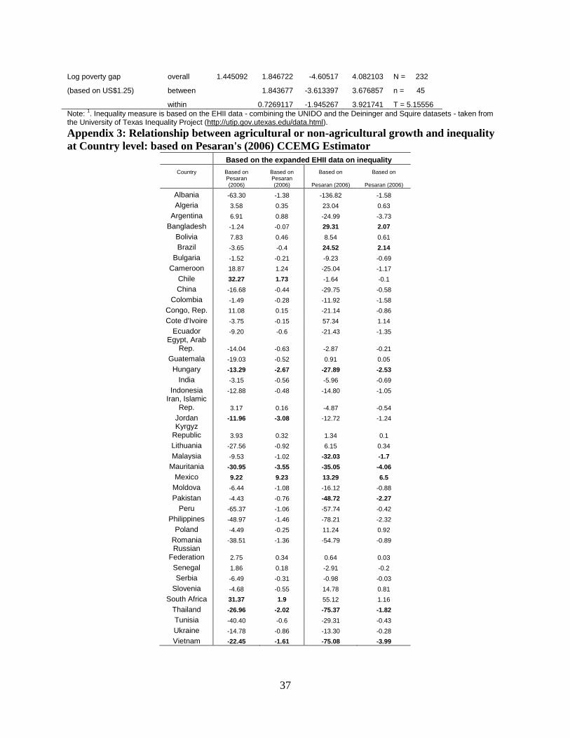
37

Log poverty gap overall 1.445092 1.846722 -4.60517 4.082103 N = 232

(based on US$1.25) between

1.843677 -3.613397 3.676857 n = 45

within

0.7269117 -1.945267 3.921741 T = 5.15556

Note: 1. Inequality measure is based on the EHII data - combining the UNIDO and the Deininger and Squire datasets - taken from

the University of Texas Inequality Project (http://utip.gov.utexas.edu/data.html).

Appendix 3: Relationship between agricultural or non-agricultural growth and inequality

at Country level: based on Pesaran's (2006) CCEMG Estimator

Based on the expanded EHII data on inequality

Country Based on Based on Based on Based on

Pesaran (2006)

Pesaran (2006) Pesaran (2006) Pesaran (2006)

Albania -63.30 -1.38 -136.82 -1.58

Algeria 3.58 0.35 23.04 0.63

Argentina 6.91 0.88 -24.99 -3.73

Bangladesh -1.24 -0.07 29.31 2.07

Bolivia 7.83 0.46 8.54 0.61

Brazil -3.65 -0.4 24.52 2.14

Bulgaria -1.52 -0.21 -9.23 -0.69

Cameroon 18.87 1.24 -25.04 -1.17

Chile 32.27 1.73 -1.64 -0.1

China -16.68 -0.44 -29.75 -0.58

Colombia -1.49 -0.28 -11.92 -1.58

Congo, Rep. 11.08 0.15 -21.14 -0.86

Cote d'Ivoire -3.75 -0.15 57.34 1.14

Ecuador -9.20 -0.6 -21.43 -1.35

Egypt, Arab Rep. -14.04 -0.63 -2.87 -0.21

Guatemala -19.03 -0.52 0.91 0.05

Hungary -13.29 -2.67 -27.89 -2.53

India -3.15 -0.56 -5.96 -0.69

Indonesia -12.88 -0.48 -14.80 -1.05

Iran, Islamic Rep. 3.17 0.16 -4.87 -0.54

Jordan -11.96 -3.08 -12.72 -1.24

Kyrgyz Republic 3.93 0.32 1.34 0.1

Lithuania -27.56 -0.92 6.15 0.34

Malaysia -9.53 -1.02 -32.03 -1.7

Mauritania -30.95 -3.55 -35.05 -4.06

Mexico 9.22 9.23 13.29 6.5

Moldova -6.44 -1.08 -16.12 -0.88

Pakistan -4.43 -0.76 -48.72 -2.27

Peru -65.37 -1.06 -57.74 -0.42

Philippines -48.97 -1.46 -78.21 -2.32

Poland -4.49 -0.25 11.24 0.92

Romania -38.51 -1.36 -54.79 -0.89

Russian Federation 2.75 0.34 0.64 0.03

Senegal 1.86 0.18 -2.91 -0.2

Serbia -6.49 -0.31 -0.98 -0.03

Slovenia -4.68 -0.55 14.78 0.81

South Africa 31.37 1.9 55.12 1.16

Thailand -26.96 -2.02 -75.37 -1.82

Tunisia -40.40 -0.6 -29.31 -0.43

Ukraine -14.78 -0.86 -13.30 -0.28

Vietnam -22.45 -1.61 -75.08 -3.99