San Jose State University San Jose State University

SJSU ScholarWorks SJSU ScholarWorks

Master's Theses Master's Theses and Graduate Research

Fall 2009

Dodge-Romig sampling plans: Misuse, frivolous use, and Dodge-Romig sampling plans: Misuse, frivolous use, and

expansion for usefulness. expansion for usefulness.

Avik Ganguly San Jose State University

Follow this and additional works at: https://scholarworks.sjsu.edu/etd_theses

Recommended Citation Recommended Citation Ganguly, Avik, "Dodge-Romig sampling plans: Misuse, frivolous use, and expansion for usefulness." (2009). Master's Theses. 4002. DOI: https://doi.org/10.31979/etd.xg3b-dgwr https://scholarworks.sjsu.edu/etd_theses/4002

This Thesis is brought to you for free and open access by the Master's Theses and Graduate Research at SJSU ScholarWorks. It has been accepted for inclusion in Master's Theses by an authorized administrator of SJSU ScholarWorks. For more information, please contact scholarworks@sjsu.edu.

DODGE-ROMIG SAMPLING PLANS: MISUSE, FRIVOLOUS USE, AND EXPANSION FOR USEFULNESS

A Thesis

Presented to

The Faculty of the Department of Industrial and Systems Engineering

San Jose State University

In Partial Fulfillment

of the Requirements for the Degree

Master of Science

by

Avik Ganguly

December 2009

UMI Number: 1484360

All rights reserved

INFORMATION TO ALL USERS The quality of this reproduction is dependent upon the quality of the copy submitted.

In the unlikely event that the author did not send a complete manuscript and there are missing pages, these will be noted. Also, if material had to be removed,

a note will indicate the deletion.

UMT UMI 1484360

Copyright 2010 by ProQuest LLC. All rights reserved. This edition of the work is protected against

unauthorized copying under Title 17, United States Code.

ProQuest LLC 789 East Eisenhower Parkway

P.O. Box 1346 Ann Arbor, Ml 48106-1346

©2009

Avik Ganguly

ALL RIGHTS RESERVED

SAN JOSE STATE UNIVERSITY

The Undersigned Thesis Committee Approves the Thesis Titled

DODGE-ROMIG SAMPLING PLANS: MISUSE, FRIVOLOUS USE, AND EXPANSION FOR USEFULNESS

by Avik Ganguly

APPROVED FOR THE DEPARTMENT OF INDUSTRIAL AND SYSTEMS ENGINEERING

t^o /Un/. 4 , -^D?

Dr. H.S.Jacob Tsao, Department of Industrial and Systems Engineering Date

<W>aJhJ h]p\j. Q i zooy

Dr. Minnie Patel, Department of Industrial and Systems Engineering Date

*23£ hlcv 6, aoo'j

Maryam Talakoob, Application Systems Engineer, Wells Fargo, CA 94105 Date

. . ^PROVED FOR THE UNIVERSITY

H i C i o

Associate Dean Office of Graduate Studies and Research Date

ABSTRACT

DODGE-ROMIG SAMPLING PLANS: MISUSE, FRIVOLOUS USE, AND EXPANSION FOR USEFULNESS

by Avik Ganguly

The Dodge-Romig plans and the Military Standard 105 Plans are the most popular

published sampling plans covered in detail in many standard textbooks on statistical

quality assurance such as Introduction to Statistical Quality Control by Douglas C.

Montgomery. In this thesis, we focus on Dodge-Romig AOQL plans. The Dodge-Romig

AOQL plans are designed to minimize the average total inspection (ATI) for a given

AOQL and a specified process average. It is argued that the Dodge-Romig plans as

currently tabulated (particularly in the standard publications or textbooks on acceptance

sampling), are not useful. However, they can be made useful if the plans focus on ranges

of the (incoming) process-average values that are greater than the target AOQL. Whether

one knows the exact value of process average p or just the exact range of the process

averages containing an uncertain p, one can use the pair of (n, c) listed under the

corresponding range to ensure the target AOQL with the minimum ATI. The thesis

provides example expansions of some of the published Dodge-Romig AOQL plans. A

new concept of certainty line is also developed which is a measure of process-average (p)

associated with gamma risk (y) whose numerical value is 0.000033. For any given lot

size if the calculated or knowledge base process-average of a manufacturer falls below or

equal to the value of the certainty line, then one would not be required to consider any

sampling plan to achieve a worst case outgoing quality.

ACKNOWLEDGEMENT

Foremost, I would like to express my sincere gratitude to my advisor Dr.

H.SJacob Tsao for the continuous support of my MS study and research, for his patience,

motivation, enthusiasm, and immense knowledge. His guidance helped me throughout

the research and writing of this thesis. I could not have imagined having a better advisor

and mentor for my graduate study.

I would like to thank Dr. Minnie Patel for her constant encouragement and

insightful comments.

My sincere thanks also go to Ms. Maryam Talakoob, who has made her support

available in a number of ways, and without whom my thesis would have been

incomplete.

I am indebted to my colleagues at Wells Fargo, Inc., in particular Mr. John Nevins

and Mr. Alex Pajarillo, for providing me constant strength and support in many possible

ways.

This thesis would not have been possible without the immense moral support

from my friend Kavitha Thomas who gave me the necessary confidence when faced with

difficulty.

This thesis is dedicated to my parents Prof. Haradhan Ganguly and Prof. Tripti

Somadder, whose constant love and prayers have given me the desire to reach higher.

v

TABLE OF CONTENTS

LIST OF TABLES vii

LIST OF SYMBOLS viii

LIST OF ABBREVIATIONS ix

CHAPTER 1 INTRODUCTION 1

CHAPTER 2 FUNDAMENTAL CONCEPTS 4

CHAPTER 3 THE DODGE-ROMIG SAMPLING PLAN (AOQL): MISUSE 8

CHAPTER 4 THE DODGE-ROMIG SAMPLING PLAN (AOQL): 11

FRIVOLOUS USE

CHAPTER 5 THE DODGE-ROMIG SAMPLING PLAN (AOQL): 12

EXPANSION FOR USEFULNESS - CERTAINTY LINE

CHAPTER 6 THE DODGE-ROMIG SAMPLING PLAN (AOQL): 17

EXPANSION OF TABLES

CHAPTER 7 CONCLUSION AND FUTURE SCOPE OF RESEARCH 19

REFERENCES 21

APPENDIX A PROGRAM TO OUTPUT (N,C) PAIRS FOR ANY GIVEN 22

LOT SIZE WHICH MEETS TARGET AOQL OF 3.0%

APPENDK B LIST OF (N,C) PAIRS WHICH MEET THE TARGET AOQL 34

OF 3.0% FOR A GIVEN LOT SIZE OF 8500

APPENDIX C SAMPLE API CALCULATION FOR THE RANGE 35

CONTAINING INCOMING PROCESS-AVERAGE FROM 3.01

TO 3.60%

VI

LIST OF TABLES

Table 3.1 Single Sampling Plan for AOQL = 3.0% 8

Table 5.1 Certainty Line for Lots with Different Lot Size 17

Table 6.1 Example Expansion of Dodge-Romig AOQL Plans 19

vn

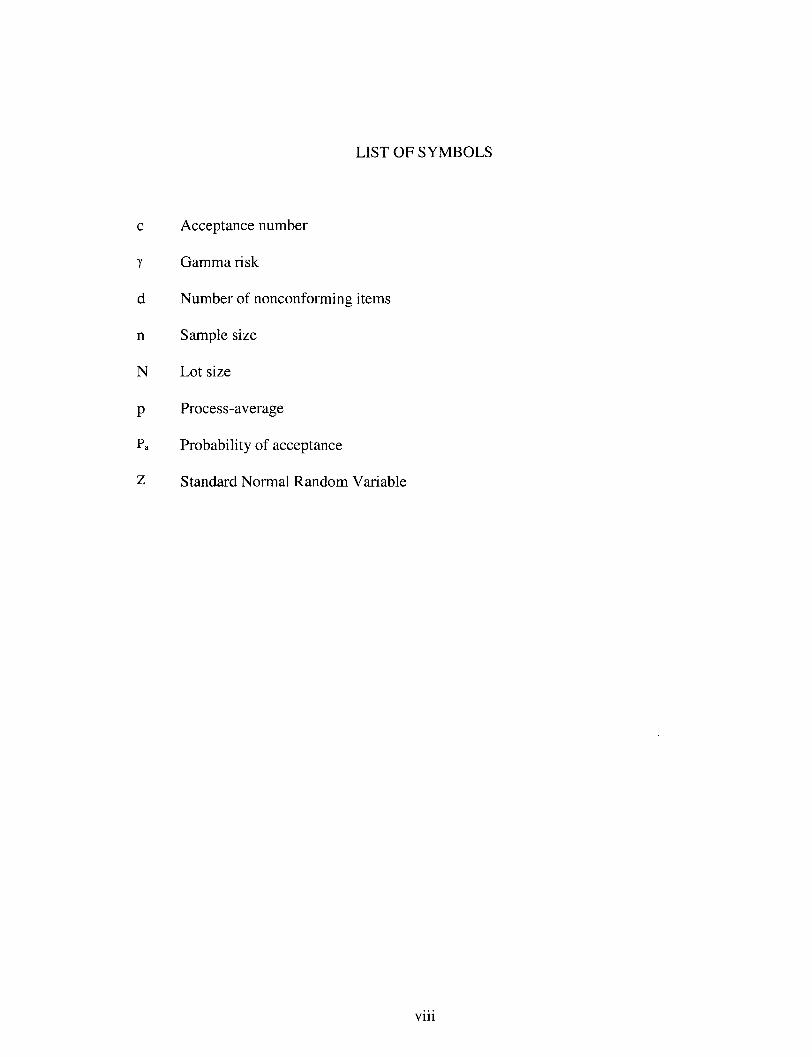
LIST OF SYMBOLS

c Acceptance number

7 Gamma risk

d Number of nonconforming items

n Sample size

N Lot size

p Process-average

Pa Probability of acceptance

Z Standard Normal Random Variable

vm

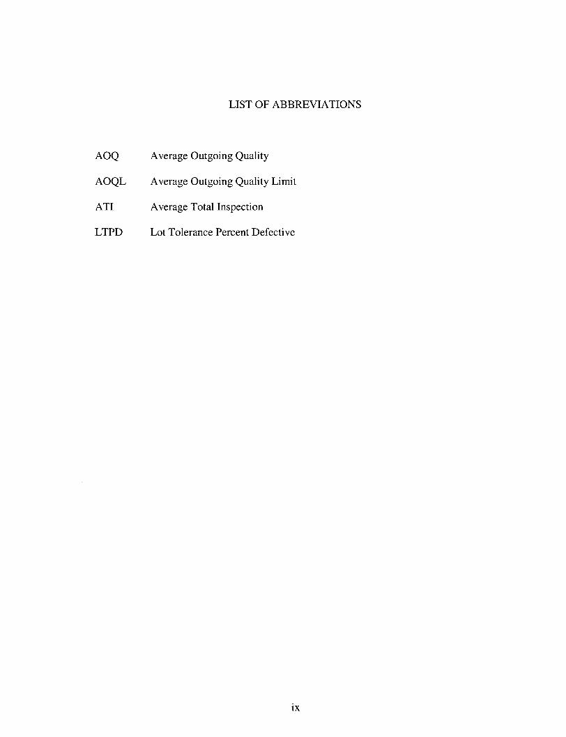
LIST OF ABBREVIATIONS

AOQ Average Outgoing Quality

AOQL Average Outgoing Quality Limit

ATI Average Total Inspection

LTPD Lot Tolerance Percent Defective

CHAPTER 1

INTRODUCTION

Although statistical process control has been the centerpiece for modern statistical

quality assurance, acceptance sampling remains a useful tool for a company to control the

quality of raw materials or parts shipped from the suppliers, particularly when no

company representatives are present at the suppliers' manufacturing facilities. Among

the categories of single, multiple, and continuous sampling plans, single sampling plans

are effective and most popular. In addition to the fundamental single sampling where the

sample size n and acceptance number c are to be determined by user-specified the AQL

and LTPD and the corresponding producer's and buyer's risk levels, the Dodge-Romig

plans and the Military Standard 105 Plans are the most popular published sampling plans

and are covered in detail in many standard textbooks on statistical quality assurance. In

this thesis, after pointing out a common misuse of the Dodge-Romig plans as well as a

common frivolous use, I propose an expansion of any of the published Dodge-Romig

plans and address the resulting usefulness.

The thesis focuses on Dodge-Romig AOQL plans. Each of the published plan tables

corresponds to a target AOQL and contains several columns corresponding to a set of

non-overlapping ranges of process-average p (i.e., incoming quality or incoming

percentage of non-conforming) and a number of rows corresponding to the same number

of non-overlapping lot-size ranges. Note that the non-overlapping ranges of process-

average p constitute the entire interval between 0 and the target AOQL. In particular, all

the process-average (p) values of all the listed ranges are smaller than the target AOQL.

For illustration purposes, we focus on the single sampling plan published for AOQL =

3.0% and focus on the lot size 8500. A single sampling is specified by a pair of n and c,

where n denotes the sample size and c denotes the acceptance number or the critical

number. A lot is accepted if the number of defective items among the n sampled items is

no greater than c. Each of the pairs of (n, c) listed for lot size 8500 guarantees an AOQL

of 3.0%, but the («, c) pair listed under the process-average range of (0.00% - 0.06%), for

example, should be selected if the process-average p falls within this range. This

particular pair produces the minimum ATI approximately, among all the (n, c) pairs listed

for lot size 8500. A common misuse of this plan or any other Dodge-Romig AOQL plan

can be illustrated as follows. "Furthermore, to use the plans, we must know the process

average [...]." (Montgomery 682). This is a misuse, and one does not have to know

exactly what the (incoming) process-average p is. Had one known the exact value of the

process-average p and had one known that this process-average p is less than 3.0%, there

is no need to conduct the sampling to begin with. This is because the 100% rectifying

inspection of the Dodge-Romig plans guarantees that the outgoing quality will be strictly

better than the (incoming) process-average. Note again that all the process-average

values of all the process-average ranges of a Dodge-Romig plan are smaller than the

target AOQL. If the process-average p is indeed 0.0006 (i.e., 0.06%), why would want to

bother with any sampling plan at all to achieve a 0.03 (i.e., 3%) worst-case outgoing

quality? (3.0% is 50 times worse than 0.06 %.) This misconception results from the fact

that ATI is a function of the (incoming) process-average p and calculation of ATI for

range selection requires the value of p. I will provide numerical examples to illustrate

how minute the probability is for any particular lot of 8500 to have 3.0% rate of

nonconforming (i.e., 255 defective items) if the process-average p is indeed 0.0006 (i.e.,

0.06%).

Some theoreticians or practitioners suggest the following frivolous use of Dodge-

Romig plans. Although one does not have to know the exact value of the (incoming)

process-average p, he/she only needs to know exactly which of the ranges listed for the

given lot size contains p and should use the (n, c) pair of the corresponding range (i.e.,

column). In this use, although the exact knowledge of the (incoming) process-average/?

is not needed, one must have the exact knowledge of the range. This use is frivolous

because, once again, had one known exactly that the process-average is within a given

listed range, there is no need for the sampling. Once again, this is because the rectifying

inspection guarantees that the outgoing quality is strictly better than the incoming

process-average. Note again that all the process-average values of all the process-

average ranges of a Dodge-Romig plan are smaller than the target AOQL.

CHAPTER 2

FUNDAMENTAL CONCEPTS

Single-Sampling Plan

A single-sampling is defined by the three entities namely lot size N, sample size n and

acceptance number c. Thus for a lot size of TV a random sample of n units is inspected

and the number of nonconforming items d is observed. If the number of nonconforming

items d is less than or equal to acceptance number c, the lot will be accepted. On the

other hand, if d > c then the lot will be rejected.

Probability of Acceptance

The probability of acceptance Pa is the probability that d < c. It is a probabilistic

measure and the result can vary from 0 to 1. It is also used in the calculation of AOQ and

ATI. Pa is large (in the order of 0.9 and more) when the incoming process-average is

low.

Percent Defective

Percent defective is a measure of quality in terms of percentage. It can vary from 0%

to 100%. It is also termed as fraction defective. It represents the number of defective

items per 100 items present in a lot of size TV. In my thesis, it is mainly referred as

incoming process-average p. This is a quality measure which defines the incoming lot

from a supplier.

Concept of Rectifying Inspection

The phenomenon of 100% screening or inspection of rejected lots forms the basis of

rectifying inspection technique. In case of a lot being sentenced, all the discovered

defective items are either removed for subsequent work or they are returned to the

supplier or replaced with a stock of good items. For example if the incoming lots have a

fraction defective of p0 then some of these lots will be accepted and some of them will be

rejected. The outgoing quality of the accepted lots will have a fraction defective of p0.

However, the rejected lots will be screened and their final fraction defective will be zero

which is definitely less than p0 since p0 is a positive real number. The overall outgoing

lots thereby are combination of lots with fraction defective p0 and fraction defective zero.

Therefore, the outgoing lots from the inspection activity will have a fraction defective

measure of say pi which is less than p0. In short, rectifying inspection is a technique

which guarantees an overall outgoing quality of lots which is strictly greater than the

overall quality of the incoming ones. The Dodge-Romig sampling plans hold good only

if rectifying inspection is adopted.

Average Outgoing Quality (AOQ)

AOQ is the measure of quality in the lot that results from the application of rectifying

inspection.

AOQ can be illustrated as follows: "It is simple to develop a formula for average

outgoing quality (AOQ). Assume that the lot size is N and that all discovered defectives

are replaced with good units. Then in lots of size N, we have

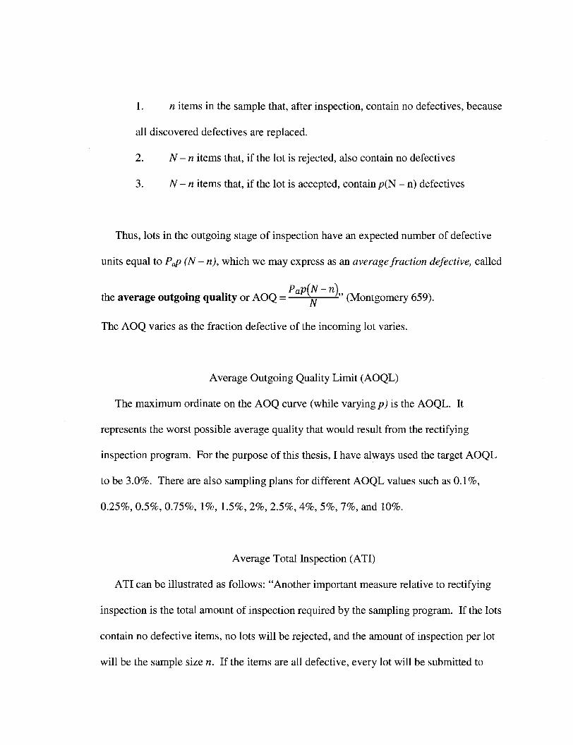
1. n items in the sample that, after inspection, contain no defectives, because

all discovered defectives are replaced.

2. N-n items that, if the lot is rejected, also contain no defectives

3. N-n items that, if the lot is accepted, contain p(N - n) defectives

Thus, lots in the outgoing stage of inspection have an expected number of defective

units equal to Pap (N-n), which we may express as an average fraction defective, called

Pap(N - n) the average outgoing quality or AOQ = JJ -" (Montgomery 659).

The AOQ varies as the fraction defective of the incoming lot varies.

Average Outgoing Quality Limit (AOQL)

The maximum ordinate on the AOQ curve (while varying p) is the AOQL. It

represents the worst possible average quality that would result from the rectifying

inspection program. For the purpose of this thesis, I have always used the target AOQL

to be 3.0%. There are also sampling plans for different AOQL values such as 0.1%,

0.25%, 0.5%, 0.75%, 1%, 1.5%, 2%, 2.5%, 4%, 5%, 7%, and 10%.

Average Total Inspection (ATI)

ATI can be illustrated as follows: "Another important measure relative to rectifying

inspection is the total amount of inspection required by the sampling program. If the lots

contain no defective items, no lots will be rejected, and the amount of inspection per lot

will be the sample size n. If the items are all defective, every lot will be submitted to

100% inspection, and the amount of inspection per lot will be the lot size N. If the lot

quality is 0 < p < 1, the average amount of inspection per lot will vary between the

sample size n and the lot size N. If the lot is of quality p and the probability of lot

acceptance is Pa, then the average total inspection per lot will be:

ATI = n + (1- PaXN-n)" (Montgomery 661).

CHAPTER 3

THE DODGE-ROMIG SAMPLING PLAN (AOQL): MISUSE

The Dodge-Romig single sampling tables obtained from the book Sampling Inspection

Tables, Single and Double Sampling by H. F. Dodge and H. G. Romig give AOQL

sampling plans for various AOQL values ranging from 0.1% to 10%. The tables are

provided for both single and double sampling. For illustration purpose, I have focused on

the plan published for AOQL = 3% and for the lot sizes 8,500 and 75,000.

Table 3.1: Single Sampling Plan for AOQL = 3.0% (Dodge and Romig 202)

Lot Size

7001-10.000 50,001-100,000

Process Average

0 to 0.06%

n 28 28

c 1 1

Process Average

0.07 to 0.60%

n 46 65

c 2 3

Process Average

0.61 to 1.20%

n 65 125

c 3 6

Process Average

1.21 to 1.80%

n 105 215

c 5 10

Process Average

1.81 to 2.40%

n 170 385

c 8 17

Process Average

2.41 to 3.00%

n 280 690

c 13 29

I have arbitrarily chosen the row 16 and 19 of the published table. For calculation purpose I

have chosen 8,500 and 75,000 which represent the median value of the interval 7,001-10,000

and 50,001-100,000 respectively. Each of the above pairs of (n, c) for lot sizes 8,500 and

75,000 guarantees an AOQL of 3.0%. Also, these particular pairs of (n, c) produce the

minimum ATI approximately, among all the (n, c) pairs listed for lot sizes 8,500 and 75,000

respectively. However, the (n, c) pair listed under the process-average range of (0.00% -

0.06%), for example in our case (28, 1), should be selected if the process-average p falls within

this range. In order to use the plans, the text books (Montgomery) state the necessity of having

the knowledge of the process-average which can also be termed as average fraction

nonconforming of the incoming product. This is a misuse of the knowledge of incoming

process average, and I argue that one does not have to know the exact incoming process-

average p. If one knows the incoming process-average p and if/? < 3.0%, then there will not be

any necessity to adopt any sampling plan. This is because the Dodge-Romig plan is only

applicable when the rejected lots are subjected to 100% inspection. This rectifying inspection

ensures the outgoing quality of the lot will always be better than the incoming process-average.

I will use the following numerical example to defend my argument. Let us consider

the initial range of the incoming process-average p (0 to 0.06%).

Problem statement: Calculate the probability of a lot with lot size 8,500 to have 3% or

more defective items given that the incoming process-average is 0.06%.

Solution: Given lot size N = 8500

Number of defective items = 3% of 8500 = 255

Incoming process-average p = 0.06% = 0.0006

Hence for a given lot size of 8,500 let us calculate the probability of having 255 or more

number of defective items when the incoming process-average is 0.0006

To calculate,

P (X > 255)

Where X is a binomial random variable with parameters N and p.

By the principle of normal approximation to the binomial distribution (Montgomery and

Runger 132)

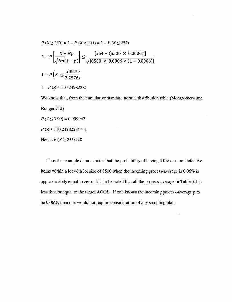
P (X> 255) = 1 -P (X< 255) = l-P(X<254)

1 - P X-Np

VWp(l-p)J

/ 248.9 \ 1-PlZ <

V - 2.2576/

[254- (8500 x 0.0006)]

V[8500 x 0.0006 x (1 - 0.0006)]

1 - P ( Z < 110.2498228)

We know that, from the cumulative standard normal distribution table (Montgomery and

Runger 713)

P(Z< 3.99) = 0.999967

P(Z<110.2498228) ~ 1

Hence P (X> 255) ~ 0

Thus the example demonstrates that the probability of having 3.0% or more defective

items within a lot with lot size of 8500 when the incoming process-average is 0.06% is

approximately equal to zero. It is to be noted that all the process-average in Table 3.1 is

less than or equal to the target AOQL. If one knows the incoming process-average p to

be 0.06%, then one would not require consideration of any sampling plan.

CHAPTER 4

THE DODGE-ROMIG SAMPLING PLAN (AOQL): FRIVOLOUS USE

The frivolous use of the Dodge-Romig sampling plan (AOQL) is quite similar to that

of its misuse. Looking back to Table 3.1, for any given range of lot size (e.g., 7,001-

10,000) there are six different non-overlapping ranges of incoming process-average p.

Some theoreticians or practitioners suggest the following frivolous use of Dodge-Romig

plans. Although for a given lot size one does not have to know the exact value of the

incoming process-average p, one must know the exact range (in our case one among the

six non-overlapping ranges listed in Table 3.1), which contains the incoming process-

average p. In this use, one must use the (n, c) pair of the corresponding range (i.e.,

column). For example, if one knows that the incoming process-average p lies within the

range of 1.21 to 1.80% and the lot size is 9,000, then one would choose (105, 5) as the (n,

c) pair for the purpose of sampling. This is a frivolous use. There is no need for

sampling if one knows that the incoming process-average p lies exactly within a given

listed range. Once again, this is because rectifying inspection guarantees that the

outgoing quality is always better than the incoming process-average. Note that all the

process-average values of all the process-average ranges of a Dodge-Romig plan are

smaller than the target AOQL.

CHAPTER 5

THE DODGE-ROMIG SAMPLING PLAN (AOQL):

EXPANSION FOR USEFULNESS - CERTAINTY LINE

Having stated the misuse and frivolous use of Dodge-Romig sampling plan, I argue

that the currently published tables can be made more useful. In this part, I am

introducing a concept of certainty line which is a measure of process-average p

associated with a gamma risk (y) whose numerical value is 0.000033. For any given lot

size if the calculated or knowledge base process-average of a manufacturer falls below or

equal to value of the certainty line then one would not require to consider any sampling

plan to achieve a worst case outgoing quality. The following numerical example will

show how we can calculate the certainty line for any given lot size.

Problem Statement: Find the process-average p such that a lot of size N will have

number of defective items being greater than or equal to N times lot percentage (in our

case AOQL of 3.0%). The probability of such measure should be smaller than or equal to

the y risk which is equal to 0.000033.

Solution: Let us consider the lot size N to be 100

Hence, the problem can be redefined as follows.

Find the process average p such that a lot size of 100 will have number of defective items

being greater than or equal to 3 (i.e. 100 x 0.03).

Given:

N=100

Lot Percentage or AOQL = 3.0%

Risk (y) = 0.000033 (Smallest number in Normal Distribution Table) (Montgomery and

Runger713)

To calculate:

P(c > 3) < 0.000033

Where c is binomial random variable with parameters N and p.

By the principle of normal approximation to the binomial distribution (Montgomery and

Runger 132)

1 - P ( c < 3 ) < 0.000033

P (( *-»P ) < ( 3 - 1 0 0 ; )) < 0.000033 \\jNp X (l-p)/ WlOOp X (l-p)/J

Multiplying both sides by -1 ,

- 1 x ! _ P (( , x~Nv ) < ( i 3-10°P ))

\\jNp x (l-p)/ VVIOOP x (i-p)//

_ 1 + p f ( X~N; ) < ( 3-10<* V\ > -0.000033 ^VV P̂ x (l-p)/ \y/l00px(l-p)JJ

Adding 1 on both sides,

P (? ™ * \ < ( 3-1 0 0^ V\ > 1 - 0.000033

P (( *-»v ) < ( 3 - ! ° ° ; V\ > 0.9999667

> - 1 x 0 . 0 0 0 0 3 3

We know that, P (Z< x) > 0.9999667 => x> 3.99(approximately) (Montgomery and

Runger713)

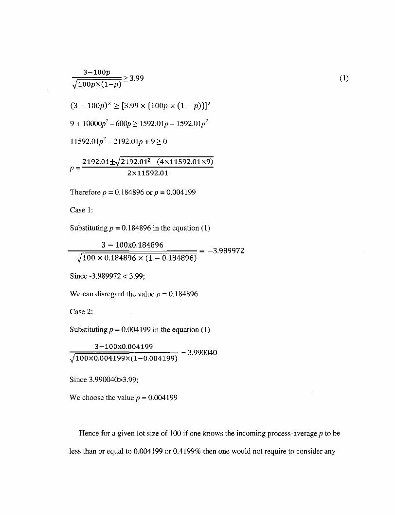
3-100p K = >3.99 VlOOpx(l-p)

(3 - 100p)2 > [3.99 x {lOOp x (1 - p)}]2

9 + lOOOOp2- 600p > 1592.01p - 1592.01p2

11592.01/?2 - 2192.01p + 9 > 0

2192.01±V2192.012-(4X11592.01X9) 77 ~ 2X11592.01

Therefore p = 0.184896 orp = 0.004199

Case 1:

Substituting p = 0.184896 in the equation (1)

3 - 100x0.184896 , = -3.989972

VlOO x 0.184896 x (1 - 0.184896)

Since -3.989972 < 3.99;

We can disregard the value p = 0.184896

Case 2:

Substituting p = 0.004199 in the equation (1) 3-100x0.004199

, = 3.990040 A/100X0.004199X(1-0.004199)

Since 3.990040>3.99;

We choose the value p = 0.004199

Hence for a given lot size of 100 if one knows the incoming process-average p to be

less than or equal to 0.004199 or 0.4199% then one would not require to consider any

sampling plan. The Table 5.1 represents some examples of various lots with different lot

size and their corresponding certainty line. Similarly, from the above numerical example

we can draw certainty line for any given lot size. In this use, one can utilize his/her

knowledge of incoming process average in order to decide whether or not he/she must

consider any sampling plan. This will improve the efficiency of sampling using Dodge-

Romig sampling plan and reduce cost by considering sampling plan only when it is

necessary in order to ensure the target AOQL.

Table 5.1: Certainty Line for Lots with Different Lot Size.

Lot Size 100 200 300 400 500 600 800 1000 2000 3000 4000 5000 7000 10000 20000 50000 100000

Certainty Line 0.41990% 0.68050% 0.86581% 1.00757% 1.11212% 1.21525% 1.36383% 1.47762% 1.81044% 1.98410% 2.09620% 2.17660% 2.28700% 2.39050% 2.55483% 2.71029% 2.79213%

Gamma Risk 0.000033 0.000033 0.000033 0.000033 0.000033 0.000033 0.000033 0.000033 0.000033 0.000033 0.000033 0.000033 0.000033 0.000033 0.000033 0.000033 0.000033

For instance, if the lot size is 100,000 then one would require considering sampling

using Dodge-Romig sampling plan only if one knows that the incoming process-average

p is greater than 2.79%. In a way, one does not have to even consider sampling for the

first five columns from Table 3.1 listing five different non-overlapping ranges of

incoming process average up to 2.40 %.

CHAPTER 6

THE DODGE-ROMIG SAMPLING PLAN (AOQL): EXPANSION OF TABLES

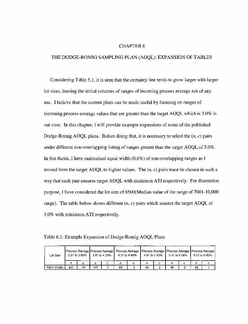
Considering Table 5.1, it is seen that the certainty line tends to grow larger with larger

lot sizes, leaving the initial columns of ranges of incoming process average not of any

use. I believe that the current plans can be made useful by focusing on ranges of

incoming process-average values that are greater than the target AOQL which is 3.0% in

our case. In this chapter, I will provide example expansions of some of the published

Dodge-Romig AOQL plans. Before doing that, it is necessary to select the («, c) pairs

under different non-overlapping listing of ranges greater than the target AOQL of 3.0%.

In this thesis, I have maintained equal width (0.6%) of non-overlapping ranges as I

moved from the target AOQL to higher values. The (n, c) pairs must be chosen in such a

way that each pair ensures target AOQL with minimum ATI respectively. For illustration

purpose, I have considered the lot size of 8500(Median value of the range of 7001-10,000

range). The table below shows different (n, c) pairs which assures the target AOQL of

3.0% with minimum ATI respectively.

Table 6.1: Example Expansion of Dodge-Romig AOQL Plans

Lot Size

7001-10.000

Process Average 3.01 to 3.60%

n 441

c 20

Process Average 3.61 to 4.20%

n 147

c 7

Process Average 4.21 to 4 80%

n 64

c 3

Process Average 4.81 to 5.40%

n 45

c 2

Process Average 5.41 to 6.00%

n 45

c 2

Process Average 6.01 to 6.60%

n 28

c 1

A program in C (Appendix A) was written to identify (n, c) pairs which establish the

target AOQL of 3.0%. It is to be noted that for every value of acceptance number c, there

exists a unique sample size n whose AOQL will be approximately equal to 3.0%.

Appendix B lists some of the («, c) pairs obtained for a given lot size of 8500, all of

which meeting the targeted AOQL of 3.0%. Note that there are only 39 pairs of (n, c)

obtained. The 39th pair of (n, c) is (848, 38). For c being 39 and onwards the

corresponding unique sample size which meets the target AOQL of 3.0% are found out to

be greater than 850. Considering those pairs for calculation and comparison of ATI adds

complexity to the process. This is because, for a lot size of 8500 the calculation of both

AOQL and ATI can rely upon binomial distribution only until n/N < 0.10. This is more

of a hypergeometric phenomenon after we exceed the sample size of 850 for a lot size

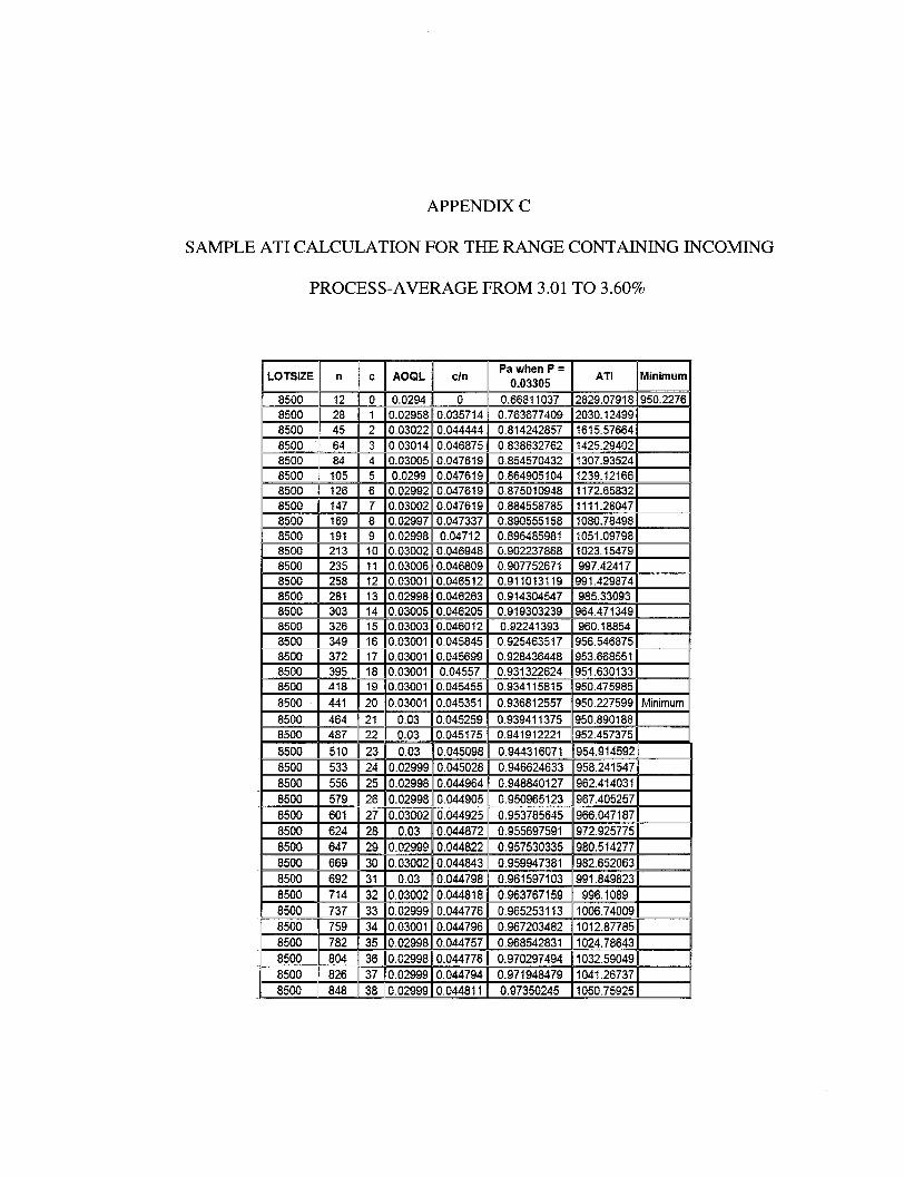
8500. Appendix C shows the sample calculation for ATI for the range of 3.01 to 3.60%.

ATI is a function of incoming process average and hence for the column 3.01 to 3.60%

the incoming process average p is considered as 3.305% which is the mean of the range

3.01 to 3.60%. For all the («, c) pairs listed in Appendix B, ATI is calculated for column

1 (3.01 to 3.60%) and each pair is compared against all the other pairs for the calculation

of minimum ATI. In this way, I provide the example expansion of already published

Dodge-Romig sampling plans.

CHAPTER 7

CONCLUSION AND FUTURE SCOPE OF RESEARCH

Conclusion

With the help of my numerical argument, it is evident that one does not have to know

the exact incoming process-average p in order to adopt a sampling plan. Not only that,

one does not even have to know the exact range which contains the incoming process-

average p in order to consider a sampling plan. However, for any given lot size N, if the

incoming process-average p is known, then one can compare the knowledge base about

the incoming process-average p against the certainty line for that given lot size and

decide whether or not he/she must consider any sampling plan. This will not only save

cost and time, but also improve the overall efficiency of a manufacturing environment.

In the case of the supplier being remotely located, such practice will help improve the

relationship of the supplier with the customer company. Dodge-Romig plans as currently

tabulated can also be made more useful by focusing upon the ranges of the (incoming)

process-average values that are greater than the target AOQL.

Future Scope of Research

A further study can be conducted to rethink the expansion of Dodge-Romig plans for

those ranges of the incoming process-average (listed in Table 6.1) which is greater than

the target AOQL. It is noteworthy that the pair of n and c which gives the minimum ATI

for the range of p from 4.81 to 5.40% is (45, 2). The similar pair provides us with the

minimum ATI for the ranges that are smaller than the target AOQL (Table 3.1: under the

range of 0.07 to 0.60%). Further research can be done to determine whether one must

consider sampling at all in cases where, for example, the required AOQL is 3% and

incoming process-averagep is known to be in the range between 4.81% and 5.40%. In

such cases, the rejection probability may be so close to one that virtually every lot is

rejected, all items of a lot are inspected, and all non-conforming items are replaced by

conforming items. Moreover, in this era of building good quality products, as opposed

to the earlier era of screening out the bad quality ones, the supplier should improve the

quality through statistical process control or be replaced by a better supplier.

REFERENCES

Dodge, Harold F., and Harry G. Romig. Sampling Inspection Tables: Single and Double

Sampling. New York: John Wiley & Sons, Inc., 1959.

Montgomery, Douglas C , and George C. Runger. Applied Statistics and Probability for

Engineers. New Jersey: John Wiley & Sons, Inc., 2007.

Montgomery, Douglas C . Introduction to Statistical Quality Control. New Jersey: John

Wiley & Sons, Inc., 2005.

The Purdue OWL. Purdue University Writing Lab, 2008. Web. 27 Dec. 2008.

APPENDIX A

PROGRAM TO OUTPUT (n, c) PAIRS FOR ANY GIVEN LOT SIZE WHICH MEETS

TARGET AOQL OF 3.0%.

#include <stdio.h>

#include <stdlib.h>

#include <string.h>

#include <math.h>

#define LINE_MAX 100

int fileFound = 0;

int printDetails = 0;

double Factorial(int n){

double fctrl= 1;

for (int i = n; i > 1; i—)

{

fctrl = fctrl * i;

}

return fctrl;

}

double SemiFactorial(int n, int j){

double sFctrl= 1;

for (int i = n; j > 0; j — , i—)

{

sFctrl = sFctrl * i;

}

return sFctrl;

}

double MathematicalCombination(int sample, int acptNbr){

double fctrlCmb;

double fctrlNC, fctrlC;

switch (acptNbr) {

case 0:

fctrlCmb = 1;

break;

case 1:

fctrlCmb = sample;

break;

default:

if (acptNbr == sample) {

fctrlCmb = 1;

}

else {

fctrlNC = SemiFactorial(sample, acptNbr);

fctrlC = Factorial(acptNbr);

fctrlCmb = fctrlNC / fctrlC;

}

break;

}

return fctrlCmb;

}

double AOQ(int lotSize, double pctD, int sample, int acptNbr){

int sampleLessAcptNbr;

double fctrlCmb;

double pPower, onePPower, probabilityAcpt, totalProbabilityAcpt, lotSizeCalc,

calculatedAOQ;

/* don't use power function when pctD is equal to 1.00 due to significant digit

error */

/* when pctD is equal to 1, AOQ is zero; (1 - pctD) raised to a power is zero when

pctD is 1 */

if (1== (int) pctD) {

calculatedAOQ = 0;

}

else {

totalProbabilityAcpt = 0;

for (int i = 0; i <= acptNbr; i++) {

fctrlCmb = MathematicalCombination(sample, i);

sampleLessAcptNbr = sample - i;

pPower = pow(pctD, i);

onePPower = pow((l - pctD), sampleLessAcptNbr);

probabilityAcpt = fctrlCmb * pPower * onePPower;

totalProbabilityAcpt += probabilityAcpt;

}

lotSizeCalc = (double) (lotSize - sample) / lotSize;

calculatedAOQ = totalProbabilityAcpt * pctD * lotSizeCalc;

}

return calculatedAOQ;

}

double CalculateAOQL(int lotSize, double pctD, int sample, int acptNbr, FILE *fDtl,

FILE *fC, FILE *fn){

double aoq, aoqMax[3];

int a, s, aMax[3], sMax[3];

double p, pMax[3];

charbuffer[200];

aoqMax[2] = pMax[2] = 0;

aMax[2] = sMax[2] = 0;

for (a = 0; a <= acptNbr; a++) {

aoqMax[l] = pMax[l] = 0;

aMax[l] = sMax[l] = 0;

for (s = (a + 1); s <= sample; s++) {

aoqMax[0] = pMax[0] = 0;

aMax[0] = sMax[0] = 0;

for (p = pctD; p < (1 + pctD); p += pctD) {

aoq = AOQ(lotSize, p, s, a);

if (printDetails) {

sprintf(buffer, "%5d %5d %5d %10.61f

%+15.10E\n", lotSize, a, s, p, aoq);

fputs(buffer, fDtl);

}

if (aoq > aoqMax[0]) {

aoqMax[0] = aoq;

aMax[0] = a;

sMax[0] = s;

pMax[0] = p;

}

}

sprintf(buffer, "%5d %5d %5d %10.61f %+15.10E

MaxPerSample(Max per C=%d n=%d)\n",

lotSize, aMax[0], sMax[0], pMax[0], aoqMax[0], a, s);

fputs(buffer, fn);

if (aoqMax[0] > aoqMaxfl]) {

aoqMaxfl] = aoqMax[0];

aMax[l] = aMax[0];

sMax[l] = sMax[0];

pMax[l]=pMax[0];

}

}

sprintf(buffer, "%5d %5d %5d %10.61f %+15.10E

MaxPerAcceptanceNbr(Max per C=%d)\n",

lotSize, aMax[l], sMax[l], pMax[l], aoqMax[l], a);

fputs(buffer, fC);

if (aoqMax[l] > aoqMax[2]) {

aoqMax[2] = aoqMax[l];

aMax[2] = aMax[l];

sMax[2] = sMax[l];

pMax[2]=pMax[l];

}

}

sprintf(buffer, "%5d %5d %5d %10.61f %+15.10E

MaxForAllAcceptanceNbrs(Max for all C)\n",

lotSize, aMax[2], sMax[2], pMax[2], aoqMax[2]);

fputs(buffer, fC);

return aoqMax[2];

}

void Usage(char *programName){

fprintf(stderr,"Usage : %s L P S A\n",programName);

fprintf(stderr," L is LotSize, P is PercentDefective, S is Sample and A is

AcceptanceNumberVi");

fprintf(stderr," or : %s -f filename\n",programName);

fprintf(stderr," filename contains LotSize, PercentDefective, Sample and

AcceptanceNumberNn");

fprintf(stderr," or : %s -p L P S A\n",programName);

fprintf(stderr," or : %s -p -f filename\n",programName);

fprintf(stderr," -p causes each aoq result to be logged to outDtl.txt\n");

fprintf(stderr,"Output: outDtl.txt - aoq details if-p option is specified\n");

fprintf(stderr," outn.txt - summary for sample\n");

fprintf(stderr," outC.txt - summary for acceptance number\n");

}

/* returns the index of the first argument that is not an option; i.e.

does not start with a dash or a slash

*/

int HandleOptions(int argc,char *argv[]){

int i,firstnonoption=0;

for (i=l; i< argc;i++) {

if (argv[i][0] == V || argv[i][0] == '-') {

switch (argv[i][l]) {

/* An argument -? means help is requested */

case '?':

Usage(argv[0]);

break;

case 'h':

case 'H':

if (!stricmp(argv[i]+l,"help")) {

Usage(argv[0]);

break;

}

/* An argument -f means the input data is in a file */

case 'f:

case 'F:

fileFound = 1;

break;

/* An argument -p means the details are written to an

output file */

case 'p':

case *P':

printDetails = 1;

break;

default:

fprintf(stderr,"unknown option %s\n",argv[i]);

break;

}

}

else {

if (firstnonoption == 0) {

firstnonoption = i;

}

}

}

return firstnonoption;

}

int main(int argc,char *argv[]){

int arglndex, argCnt, lotSize, sample, acptNbr;

char line[ 100];

FILE *f = NULL;

FILE *fh = NULL;

FILE *fDtl = NULL;

FILE *fC = NULL;

double pctD, aoqL;

// Minimum 3 arguments - input file option

if (argc < 3) {

Usage(argv[0]);

return 1;

}

/* handle the program options */

arglndex = HandleOptions(argc,argv);

argCnt = argc - fileFound - printDetails;

if (IfileFound && argCnt < 5) {

Usage(argv[0]);

return 1;

}

fn = fopen("outn.txt", "w");

if(fn==NULL) {

fprintf(stderr, "Unable to open sample output file: outn.txtW);

1

fDtl = fopenCoutDtl.txt", "w");

if (fDtl == NULL) {

fprintf(stderr, "Unable to open detail output file: outDtl.txt\n");

}

fC = fopen("outC.txt", "w");

if(fC==NULL){

fprintf(stderr, "Unable to open acceptance number output file:

outC.txt\n");

}

if(fn&&fDtl&&fC){

if(fileFound){

f = fopen(argv[arglndex], "r");

if(f==NULL){

fprintf(stderr, "File not found: %s\n", argv[arglndex]);

}

else {

while (fgets(line, LINE_MAX, f) != NULL) {

sscanf(line, "%d %lf %d %d", &lotSize, &pctD,

&sample, &acptNbr);

aoqL = CalculateAOQL(lotSize, pctD, sample,

acptNbr, fDtl, fC, fn);

}

fclose(f);

}

}

else {

lotSize = atoi(argv[argIndex]);

pctD = atof(argv[++arg!ndex]);

sample = atoi(argv[++argIndex]);

acptNbr = atoi(argv[++argIndex]);

aoqL = CalculateAOQL(lotSize, pctD, sample, acptNbr, fDtl, fC,

fn);

}

fclose(fDtl);

fclose(fC);

fclose(fn);

}

return 0;

}

APPENDIX B

LIST OF in, c) PAIRS WHICH MEET THE TARGET AOQL OF 3.0%

FOR A GIVEN LOT SIZE OF 8500

Lot Size

8500

8500

8500

8500

8500

8500

8500

8500

8500

8500

8500

8500

8500

8500

8500

8500

8500

8500

8500

8500

8500

8500

8500

8500

8500

8500

8500

Percent defective

0.0370

0.0370

0.0370

0.0370

0.0370

0.0360

0.0360

0.0360

0.0360

0.0360

0.0360

0.0360

0.0360

0.0360

0.0360

0.0360

0.0360

0.0360

0.0360

0.0360

0.0360

0.0360

0.0360

0.0360

0.0360

0.0360

0.0360

n

258

281

303

326

349

372

395

418

441

464

487

510

533

556

579

601

624

647

669

692

714

737

759

782

804

826

848

c

12

13

14

15

16

17

18

19

20

21

22

23

24

25

26

27

28

29

30

31

32

33

34

35

36

37

38

PA

0.836504638

0.837849438

0.842323601

0.843988359

0.845805943

0.871706009

0.874156535

0.876625478

0.879097998

0.881562531

0.884010196

0.886433959

0.888828635

0.891189992

0.893514931

0.897286594

0.899481297

0.901636899

0.90508008

0.907111406

0.910335243

0.912249029

0.915269673

0.917072594

0.919905066

0.922627866

0.925246179

A O Q L

0.030011227

0.029975591

0.030054998

0.0300299

0.03000989

0.030008018

0.030007223

0.03000658

0.03000558

0.030003825

0.030001018

0.029996926

0.029991377

0.029984243

0.029975427

0.030018354

0.030004155

0.029988229

0.030018417

0.029997427

0.030019214

0.02999346

0.030007493

0.02997727

0.029984143

0.029986925

0.029985813

APPENDIX C

SAMPLE ATI CALCULATION FOR THE RANGE CONTAINING INCOMING

PROCESS-AVERAGE FROM 3.01 TO 3.60%

LOTSIZE

8500 8500 8500

8500 8500 8500 8500 8500 8500 8500 8500 8500 8500 8500 8500 8500 8500 8500 8500 8500

8500

8500 8500

8500

8500

8500

8500

8500

8500

8500

8500

8500

8500

8500

8500

8500

8500

8500

8500

n

12 28 45 64 84 105 126 147 169 191 213 235 258 281 303 326 349 372 395 418 441 464 487 510 533 556 579 601 624 647 669 692 714 737 759 782 804 826 848

c

0 1 2 3 4 5 6 7 8 9 10 11 12 13 14 15 16 17 18 19 20 21 22 23 24 25 26 27 28 29 30 31 32 33 34 35 36 37 38

AOQL

0.0294 0.02958 0.03022

0.03014 0.03005 0.0299 0.02992 0.03002 0.02997 0.02998 0.03002 0.03006 0.03001 0.02998 0.03005 0.03003 0.03001 0.03001 0.03001 0.03001

0.03001

0.03 0.03

0.03

0.02999

0.02998

0.02998

0.03002

0.03

0.02999

0.03002

0.03

0.03002

0.02999

0.03001

0.02998

0.02998

0.02999

0.02999

c/n

0 0.035714 0.044444

0.046875 0.047619 0.047619 0.047619 0.047619 0.047337 0.04712 0.046948 0.046809 0.046512 0.046263 0.046205 0.046012 0.045845 0.045699 0.04557 0.045455

0.045351

0.045259 0.045175

0.045098

0.045028

0.044964

0.044905

0.044925

0.044872

0.044822

0.044843

0.044798

0.044818

0.044776

0.044796

0.044757

0.044776

0.044794

0.044811

Pa when P = 0.03305

0.66811037 0.763677409 0.814242857

0,838632762 0.854570432 0.864905104 0.875010948 0.884558785 0.890555158 0.896485981 0.902237868 0.907752671 0.911013119 0.914304547 0.919303239 0.92241393 0.925463517 0.928436448 0.931322624 0.934115815

0.936812557

0.939411375 0.941912221

0.944316071

0.946624633

0.948840127

0.950965123

0.953785645

0.955697591

0.957530335

0.959947381

0.961597103

0.963767159

0.965253113

0.967203482

0.968542831

0.970297494

0.971948479

0.97350245

ATI

2829.07918 2030.12499 1615.57664

1425.29402 1307.93524 1239.12166 1172.65832 1111.28047 1080.78498 1051.09798 1023.15479 997.42417 991.429874 985.33093 964.471349 960.18854 956.546875 953.668551 951.630133 950.475985

950.227599

950.890188 952.457375

954.914592

958.241547

962.414031

967.405257

966.047187

972.925775

980.514277

982.652063

991.849823

996.1089

1006.74009

1012.87785

1024.78643

1032.59049

1041.26737

1050.75925

Minimum

950.2276

Minimum