DOCUMENTS DE TREBALL

DE LA FACULTAT DE CIÈNCIES

ECONÒMIQUES I EMPRESARIALS

Col·lecció d’Economia

The relationship of capitalization period length with market

portfolio composition and betas

Jordi Esteve Comas (*)

Dídac Ramírez Sarrió (**) University of Barcelona

Adreça correspondència: Departament de Matemàtica Econòmica, Financera i Actuarial Facultat de Ciències Econòmiques i Empresarials Universitat de Barcelona Av. Diagonal 690 08034 Barcelona (Spain) Tel.:0034934021953-Fax:0034934034892 Email.- jesteve@ub.edu; dramirezs@ub.edu (*) Full professor at the University of Barcelona. His doctoral thesis was entitled “An approach to portfolio theory starting from linear index models. Application to Spanish mutual funds”. Member of the IAFI Group.

(**) Professor at the University of Barcelona. Head of the Department of Economic, Financial and Actuarial Mathematics. Member of the Spanish Royal Academy of Economic and Financial Sciences. Head of the IAFI Group.

Abstract:

Beta coefficients are not stable if we modify the observation periods of the returns. The market

portfolio composition also varies, whereas changes in the betas are the same, whether they are

calculated as regression coefficients or as a ratio of the risk premiums. The instantaneous beta,

obtained when the capitalization frequency approaches infinity, may be a useful tool in

portfolio selection.

JEL Classification: G11, G12

Keywords: CAPM, Period Capitalization, Beta, Portfolio Composition, Instantaneous

Beta.

Resumen:

Los coeficientes beta no son estables si se modifica la duración de los periodos en los que se

mide la rentabilidad de los activos. La composición de la cartera de mercado también varía. Los

cambios en las betas son los mismos si éstas han sido calculadas como coeficientes de

regresión o como cocientes de primas de riesgo. La beta instantánea obtenida cuando la

frecuencia de capitalización tiende a infinito puede ser utilizada como herramienta en la

selección de carteras.

1

1. INTRODUCTION

The beta of an asset i in relation to market portfolio M admits two definitions: as a

linear regression coefficient:

Covariance between returns on asset 'i' and returns on market MVariance in returns from market portfolio M

(LR)βi =

= (1)

and as a quotient of the risk premiums:

Expected return asset i - (Return risk-free asset)Expected return M - (Return risk-free asset)

Risk premium asset i Risk premium M

(E)βiEi

EM

= =

= = (2)

The Capital Asset Pricing Model (CAPM) underlies the second way of calculating

the beta coefficient above. The model assumes that betas of the different assets have

been obtained according to (1) and uses a set of hypotheses to demonstrate that the risk

premium on asset i is equal to the beta of asset i multiplied by the risk premium on the

market portfolio M. Thus, mathematically:

( ) ( )

LR E

i iβ β= (3)

So, from this expression, the following one is obtained:

( )·LRE Ei i Mβ= (4)

With the CAPM, it does not matter which of the two formulae (1) or (2) calculates

the beta. Thus, two different calculation procedures exist for any single beta. As a

consequence of (3), one usually speaks of the beta without worrying about which of the

two procedures is used.

2

Whether (1) or (2) is employed, the historical data on the distribution of the return

on the asset i need to be known. According to CAPM assumptions, for any asset i,

these returns will refer to a single period, i.e. quarterly or monthly or so forth. The

period length is constant. However, it has been proven that a change in the period

length modifies the value of the betas.1 Thus, for instance, in Meucci, A. (2005), the

beta is defined depending on the period interval. Since the betas vary, we wondered

whether, in theoretical terms, it was possible to find a functional relationship between

the betas and the period. Furthermore, no empirical observations exist on market

portfolio composition variation as a function of period length. We wondered if this

variation did indeed exist and whether it was possible to find a functional relationship

theoretically. Finally, we wondered about the limit of such a functional relationship

when the period length approaches 0.

In accordance with the CAMP assumptions and the stationarity and independence of

the return distributions in different intervals, the purpose of this paper is as follows:

• First, we establish the functional dependence between market portfolio composition

and period length (see theorem 1).

• Second, we demonstrate that there is a functional dependence between period length

and betas (see theorem 2).

• Third, we introduce the concepts of instantaneous beta and instantaneous market

portfolio and we obtain their formulae (see section “The CAPM when period length

approaches 0”).

Although this paper has a theoretical character, the aforementioned results have

practical consequences for investors. For instance, in their daily practice they have to

1 For an empirical study of this kind applied to shares in the Spanish stockmarket index, the Ibex35, see Fernandez, P. (2004).

3

consider the way the betas are calculated so as not to operate with non-homogeneous

magnitudes.

This paper is divided into five parts. First of all we state the mathematical notations

and prior assumptions. Next we obtain the market portfolio composition and, in the

third part, betas are obtained as a function of dependence on the period length. In the

fourth part, we develop the CAPM when period length approaches 0 and, specifically,

we obtain instantaneous betas. Finally, we bring together the results and suggest some

possible avenues for future development.

2. MATHEMATICAL NOTATIONS AND PRIOR ASSUMPTIONS

Given a group of N risky assets ( i I {1,2,...., }N∈ = ) and a risk-free asset 0, for assets

i I∈ , let ( ) (1 )pr i Ni ≤ ≤ be the random variable for the return on asset i in any period

length p. Let p0 be the capitalization period length, assumed to be constant and

expressed in years.

We also assume that the distribution functions of the corresponding returns

0( ) pr ri i= satisfy the following hypotheses:

(i) They are known.

(ii) For a concrete asset i I∈ , they are identical for different time intervals of length

p0.

(iii) They have finite variance.

(iv) For unconnected time intervals of period length p0, they are independent (both for a

single asset and for various assets).

4

Hypothesis (i) supposes that, as in the CAPM model, all investors operating in the

market have the same expectations; (ii) implies that these expectations are stationary,

i.e. they do not vary from one period to another; (iii) requires the variance of returns to

be finite, since otherwise (1) could not be calculated; (iv) implies that assets behave in

accordance with the random - walk.2

Let: ( ) ( ) ( )(1 ) 1 ( )p p pA E r E ri i i= + = + be the expected financial factor for a period

length p, corresponding to asset i.

Let 0( )pA Ai i=

Let ( )0

0 0p

r r= be the effective return on a risk-free asset referring to a period length

p0.

Let( ) ( )0 010 0 0p p

A A r= = + be the certain financial factor.

Let t=p/p0 (p>0 is the new period length under consideration)

It follows that for a period length p:

0( ) ( ) /1 (1 ) (1 )0 0

p p p p t tA r r r Ao o o= + = + = + = (5)

Let 01 1(p) (p) (p)E A - Ai iNx Nx

= be the column vector of the N risk premiums.

2 In addition, note that (i) gives rise to two versions of the study, depending on whether the

hypothesis is applicable or not to the market portfolio M. The first version will be the subject of

another article. Here we discuss the second version. Hypothesis (i) will only be applicable to M if it

admits the entrance of new assets and the exit of others. Otherwise, the return of M could not be

stationary, since the assets with a higher expected return would be more likely to increase their

weight in the portfolio than those assets with a lower expected return.

5

From (38) (see appendix), the vector column corresponding to the mean risk

premiums for a period length p is:

0 11(p) t tE A Ai i NxNx

= − (6)

Let ( )'p

ii NxNσ

be the covariance matrix of the N risky assets, where:

( ) ( ) ( ) ( ) ( )cov( , ) cov(1 ,1 ) (1 i N, 1 i' N)' ' 'p p p p pr r r ri iii i iσ = = + + ≤ ≤ ≤ ≤ are the

covariances of the returns on assets i and i' corresponding to one single period of length

p.

Let ( )pVi be the variance of asset i for an interval with length p.

Let 1

(p)XM,i Nx

be the market portfolio composition vector.

3. MARKET PORTFOLIO COMPOSITION AS A FUNCTION OF PERIOD

LENGTH

In the proof of the CAPM equation, the relative weights in the market portfolio of

the N assets are proportional to the vector resulting from the multiplication of the

inverse of the covariance matrix by the column vector of the risk premiums.3 Division

of the resulting vector by the sum of its components gives a vector with the sum of its

components equal to 1. This vector provides the relative weights of the different assets

in the market portfolio. If we apply the CAPM to a period length p, the result is: 4

3 For this proof, see Jaquillat (1989: 153-156). 4 Comments on expression (7):

6

( )

1

111 1 1 1

(p) (p)σ · Eij i(p) NxN NxXM,i Nx (p) (p)' · σ · ExN ij iNxN Nx

−

= − (7)

Expression (7) shows that the market portfolio composition depends on the

covariance matrix and on the vector of the risk premiums. However, both the matrix and

the vector depend on p (see (38) and (39) and bear in mind that t=p/p0). As a

consequence, the market portfolio composition depends on the length p of the period

that we are considering.

Theorem 1: The market portfolio composition is determined by the following

expression as a function of p:

1 2

1

(p)SEi(p)X (i , ,......N)N (p)M,i SEij

= =∑=

(8)

where:

( ) ( ) ( ). .11 1 1( ) ( ) ( ). .( ) 21 2 2

..... . .... . .....( ) ( ) ( ). .1

p p pE np p pEp nSEi

p p pEn nnn

σ σ

σ σ

σ σ

= (9)

a) The result of operating the numerator is an Nx1 vector whose components are proportional to the relative weights of the N assets in the market portfolio. b) (1) ' Nx1 represents a row vector whose components are all equal to 1. c) The result of operating the denominator is a 1x 1 matrix (in fact it is a real number). It is possible to prove that this number is the sum of the components of the vector obtained in the numerator. d) As a consequence, the final result is a vector whose components add up to 1.

7

is the determinant of the matrix resulting from the replacement, in the covariance

matrix, of the vector of the risk premiums by the ith column.5

Proof: Let us consider the system of N+1 equations in N unknowns:

( ) ( )'( ) ·( ) ·( ),1 1( ) ( ) ( )· · ,( ) ( ) ( )' 1( ) ·( ) ·( ), ,1 1 1 2

( ) 1,1

p pe X Ni ij NxN M jxN Nxp p pE X EiM ií p p p iX XijM i NxN M jxN Nx(i , ......N)

N pX M ii

σ

σ

= ∑=

=

=∑=

(10)

In the above expression, (ei) is the ith vector of the canonical base of Rn (i.e., it is a

vector that has all its components equal to zero except the ith component, which is equal

to 1).

The first N equations are a consequence of the CAPM equation (the fraction is the

beta and the parenthesis is the market risk premium). The last equation establishes that

the sum of the weight of the N assets must be 1.

Starting from the previous equation system, by dividing equations 2 to N by the first

equation, the following linear system is obtained:

5Comment on proposition:

a) What happens if application of formula (8), which provides the market portfolio composition, gives a negative weight (Xi <0)? Concrete examples demonstrate that this is mathematically possible, but while an individual portfolio can have some negative weights, the market portfolio must have, by definition, no negative weights. b) A possible solution to the problem outlined in point a) is to discard the assets that provide negative weights (thus, Xi=0 for the assets with initially negative weights) and to repeat of the calculation of the formulas of theorem 1, without the rows and columns for the assets with initially negative weights. The aim is to find the best possible approach for choosing the most appropriate solution from the non-negative solutions that satisfy systems (10) and (11).

8

( ) ( )·( ) ,1 2 ( ) ( ) ( )· 1 ,11

( ) 1,1

N p pXp ij M jE jí (i ......N)Np p pE XM jjjN pXM ii

σ

σ

∑== =∑=

=∑=

(11)

Solution of this system gives the solutions determined by expressions (8). It can easily

be confirmed that these solutions satisfy equations systems (10) and (11), if one bears in

mind the following result:

( ) ( ) ( ) ( )· ·1

N p p p pSE Eij j i ij NxNjσ σ=∑

= (12)

4. THE BETA AS A FUNCTION OF PERIOD LENGTH

Theorem 2:

a) Betas of the assets also depend on p.

b) For any p, the betas of the diverse assets are proportional to the respective risk

premiums.

This can be expressed as follows:

( )

1' ( ) ( ) 1 · · ' '1( ) ( )1 ' 11 1( ) ( ) ( )· ·1 1

p pEij ixNp pNxN Nx Ei ixN xNp p pE Ei ij ixN NxN Nx

σβ

σ

−

= − (13)

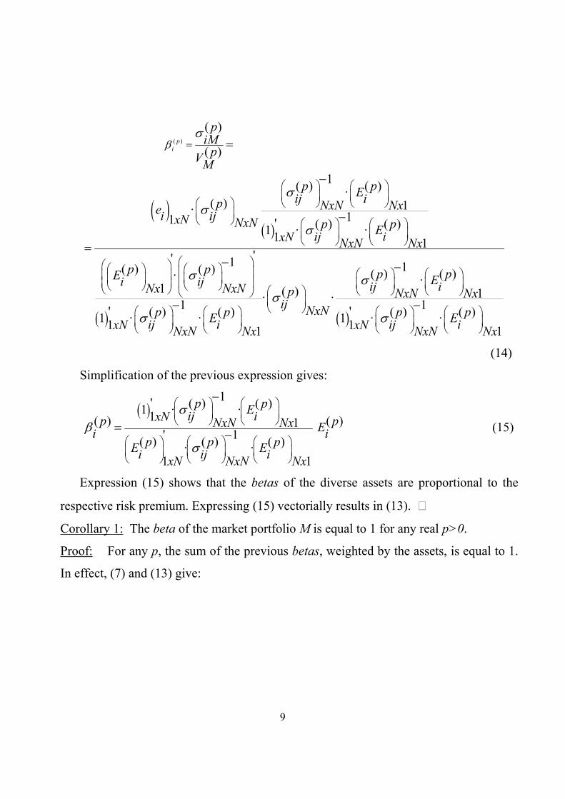
Proof:

We begin with the expression:

9

( )

( )

( )

( ) ( )

( )

1( ) ( )·( ) 1· 11 ' ( ) ( )1 · ·1 1

'' 1( ) ( )·1

'1 ·1

pi

piM

pVM

p pEij ip NxN Nxei ijxN NxN p pEij ixN NxN Nx

p pEi ijNx NxN

xN

βσ

σσ

σ

σ

=

=

−

−

=−

( )

1( ) ( )·( ) 1· ·1 1'( ) ( ) ( ) ( )· 1 · ·11 1

p pEij ip NxN Nxij NxNp p p pE Eij i ij ixNNxN Nx NxN Nx

σσ

σ σ

−

− −

(14)

Simplification of the previous expression gives:

( )

1' ( ) ( ) 1 · · 1( ) ( )1 ' 1( ) ( ) ( )· ·1 1

p pEij ixNp pNxN Nx Ei ip p pE Ei ij ixN NxN Nx

σβ

σ

−

= − (15)

Expression (15) shows that the betas of the diverse assets are proportional to the

respective risk premium. Expressing (15) vectorially results in (13).

Corollary 1: The beta of the market portfolio M is equal to 1 for any real p>0.

Proof: For any p, the sum of the previous betas, weighted by the assets, is equal to 1.

In effect, (7) and (13) give:

10

( )

'( ) ( ) ( ) ( )·, ,1 111( ) ( )' 1 · · '1 ( )1 ·' 1 1( ) ( ) ( )· ·

1 1

N p p p pX Xi iM i M ixN Nxip pExN ij i pNxN Nx Ei xNp p pE Ei ij ixN NxN Nx

β β

σ

σ

= =∑=

−

= ⋅−

( )

1( ) ( )·( )1· 1 1( ) ( )'1 · ·1 1

p pEij i pNxN NxMp pExN ij iNxN Nx

σβ

σ

−

= =− (16)

Corollary 2: For any real p we have

( )

( )( )

pEp ii pEM

β = (17)

Proof: From (7), the risk premium on the market portfolio is obtained by weighting

the risk premium of the N assets:

( )

( )

'( ) ( ) ( ) ( ) ( )· ·. ,1 111( ) ( )·'( ) 1

11 ' ( ) ( )1 · ·1 11' ( ) ( )1 · ·11 1

( ) ( )

Np p p p pE X E E Xi iM M i M ixN N xi

p pEij ip N xN N xEi xN p pEij ixN N xN N x

p pEij ixN N xN N xpE pM Ei

σ

σ

σ

= = =∑=

−

= ⇒−

−

⇒ = (18)' 1( ) ( )· ·1 1

p pEij ixN N xN N xσ

−

By applying (18) to (15), we obtain (17)

11

Corollary 3: For any real positive p the beta obtained as a regression coefficient

coincides with the beta obtained as a quotient of the risk premiums.

Proof: It is possible to calculate the beta as a regression coefficient directly as a

quotient of the risk premiums:

( ) ( ) ( )( )

'( ) ( ) ( ) ( ) ( )· ·, ,1 1 1

p p pE E Ep i i ii Np p pE p pX EM E XiM i i M ii xN Nx

β

= = =∑=

(19)

Application of (7) gives:

( )

( )

( )( )

1( ) ( )·'( ) 111 ' ( ) ( )1 · ·1 1

1' ( ) ( ) 1 · · 1 ( )1 ' 1( ) ( ) ( )· ·1 1

pEp ii p pEij ip NxN NxEi xN p pEij ixN NxN Nx

p pEij ixN pNxN Nx Eip p pE Ei ij ixN NxN Nx

βσ

σ

σ

σ

= =−

−

−

= ⋅− (20)

which is identical to (15)

5. THE CAPM WHEN PERIOD LENGTH APPROACHES 0

If we calculate the following limits:

12

( )

1' ( ) ( ) 1 · · 1( ) ( )1 ' 1p 0 0 ( ) ( ) ( )· ·1 1

p pExN ij ip pNxN NxLim Lim Ei ip p p pE Ei ij ixN NxN Nx

σβ

σ

−

= −→ → (21)

( )

1( ) ( )·( ) 1 , 1p 0 01 ' ( ) ( )1 · ·1 1

p pEij ip NxN NxLim X LimM i pNx p pEij ixN NxN Nx

σ

σ

−

= −→ → (22)

we obtain the instantaneous beta ( )INSTiβ

and the instantaneous market portfolio

composition ( )INSTXi

, respectively.

When calculating the limit when p approaches 0 in (19) and applying L’Hôpital’s rule,

we obtain:

( ) 0 0( ) 0·, 01

INST i ii N INST MX jM jj

ρ ρ ρ ρβ

ρ ρρ ρ

− −= =

−−∑

=

(23)

where:

( )( ) ; ( ) ; ·,0 1

N INSTLn A Ln A Xi i o jM M jjρ ρ ρ ρ= = = ∑

= (24)

In addition, we obtain the instantaneous market portfolio composition by calculating

the limit, when p approaches 0, through applying both L’Hôpital’s rule N times and the

derivation rules for determinants on (8):

( )( ) (i 1,2,......N)

( )1

INSSEiINSXi N INSSEij

= =∑=

(25)

13

where:

111 11 ... ... 12 ·0 11

221 21 ... ... 1( ) · ·2 1 0 2................. ... ............ ... ................

11· 1

A NLn Ln LnA A AA N

A NLn Ln LnINS A A A A ASE Ni

NLnA AN

σσ

σσ

σ

+ +

+ +=

+ ... ... 1 20

AN NNLn LnA AN

σ

+

(26)

Using the instantaneous market portfolio and instantaneous betas has the advantage

that the value of the above mentioned magnitudes does not depend on the initial period

p0. Thus, the limits mentioned above enable us to unify criteria when dealing with the

variables related to the CAPM.

6. CONCLUSIONS

When the CAPM is applied to a group of N assets assumed to have stationary and

independent return distributions, for different periods, the results obtained depend on

the period length p. In short, when p varies, the following variables also change:

• The market portfolio composition vector.

• The risk premium on the N assets.

• The risk premium market return.

• Betas of each of the N assets.

Therefore, we have as many CAPM models as positive values of p.

14

The market portfolio composition vector and the vector of the betas of the diverse

assets vary, inasmuch as the period length varies in which the returns on the assets are

measured. In particular, expressions (7) and (13) show these results, which provide, as

a function of p, the market portfolio composition and the vector of the betas

respectively. In both expressions, the inverse of the covariance matrix and the vector of

the risk premiums intervene.

The limit when p approaches 0 is relevant. In this case, we will obtain instantaneous

betas and the instantaneous market portfolio composition.

The following requires further study:

a) The vectorial function:

( )

1

NR Rpp i Nx

β

+ →

→ (27)

as well as each of the components of this vectorial function (they are real functions of a

real variable).

b) The vectorial function:

( ) , 1

NR Rpp XM i Nx

+ →

→ (28)

as well as each of the components of this vectorial function (they are real functions of a

real variable).

c) It is particularly important to study the intervals in which the components

increase and decrease, as well as the limits at zero and infinity relating to each

component of the two previous vector functions, using the risk premiums and the

covariances between the various assets. It would be interesting to analyse whether the

evolution of the variables linked to the assets with a beta below 1 is qualitatively

15

different from that of the assets with a beta larger than 1. It would also be useful to

analyse the behavior of possible negative betas.

The greatest difficulty in achieving these three objectives lies in obtaining, for any p,

the general expression of the inverse of the covariance matrix and, in particular, its limit

when p approaches 0.

16

APPENDIX

Set out below are the statistical properties of the means, variances and covariances

when modifying the period length p in which returns are measured. In the properties

A1) and A2) of this appendix we do not suppose that the returns on assets are

stationary.

A) Properties for period length K·p0 (K positive integer).

01 1 1 ,1

K(K·p )) E( r ) ( E(r ))i i jj+ = +∏

= (29)

(( )0,p

ri j is the return on asset i in the period j of length p0)

Proof: Since the random variables are independent of each other, following Cramer

(1962:23) the expectation of the product is a product of expectations, as a result of

which the property is demonstrated.

1 ') corollary: If the random variables corresponding to every period j of length p0 have

the same distribution, Ai,j=Ai, then we have the following result:

0( · )(1 )1

KK p KE r A Ai i ij+ = =∏

= (30)

0 0 0 0 0 0( · ) ( ) ( ) ( ) ( ) ( ) 2) , ,' ', , ',1 1

K KK p p p p p pσ σ A ·A - A ·Ai j i jii ii j i' j i jj j

= +∏ ∏= =

(31)

(( )0

',p

ii jσ is the covariance between the returns on assets i and i’ in the period j with

length p0)

17

Proof:

0 0 0 0 0( · ) ( · ) ( ) ( · ) ( )1 · 1, ' ,1 10 0 0 0( · ) ( · ) ( ) ( )1 1 ·,' ,1 10 0( ) ( )(1 )·(1 ), ',1

K KK p K p p K p pσ E ( r A )( r A )i i jii' i i' jj jK KK p K p p pE r r A Ai i ji i' jj j

K p pE r ri j i jj

= + − + − =∏ ∏= =

= + ⋅ + − =∏ ∏= =

= + +∏=

0 0( ) ( )·, ,1 10 0 0 0( ) ( ) ( ) ( )(1 )·(1 ) · , ,', ,1 1 1

K Kp pA Ai j i' jj jK K Kp p p pE r r A Ai j i ji j i' jj j j

− =∏ ∏= =

= + + − =∏ ∏ ∏= = =

0 0 0 0 0( ) ( ) ( ) ( ) ( )· ·, ,, ', ,1 1

K Kp p p p pσ A A A Ai j i jii' j i j i' jj j

=

+ −∏ ∏= =

2 ') corollary: If the random variables are stationary - i.e. if for every period of length p

they have the same distribution - we have:

( ) ( )0( · ) ( ) · ·, ,' ', , , ' ' '1 1

K KK KK p A ·A A ·A A A A Ai t i t i iii ii t i' t i' t ii i it tσ σ σ= + − = + −∏ ∏

= = (32)

0( · ) 2 K 2 3) V (V A ) -Ai i i

K p Ki= + (33)

Proof: This is the result of property 2 ', making i=i '

B) Properties for period length p0/m (m positive integer).

In this section it is assumed that the distributions of returns on the various assets are

stationary for periods of length p0/m.

18

0 1 1) 1 (p /m) /m E( r ) Ai i+ = (34)

Proof: On applying property 1 of section A), taking K=m, we have:

0 0( / ) ( / ) 1/ E(1 ) E(1 ) E(1 )m

p m p m mr r A r Ai i i i i

+ = + = ⇒ + =

0 0( / ) ( ) 1/ 1/ 2) ' ' 'p m p m mσ (σ A ·A ) -(A A )i iii ii' i i= + (35)

Proof: On applying property 2 ' of section A), making K=m, and property 1B), we have:

0 0( ) 1 1 1 1 )p (p /m) /m /m m /m /m m σ (σ A ·A ) -(A ·Ai iii' ii' i' i'= + (36)

On solving 0( / )'p m

iiσ we have the equality that we sought to demonstrate.

0 0( / ) ( ) 2 1/ 2/ 3) p m p m mV (V A ) - Ai i i i= + (37)

Proof: This results directly from property 2) above, taking i'=i.

C) Properties for period length p (p=t·p0, t positive real).

In this section we assume that the distributions are stationary. By combining the

properties of A) and B) in this appendix, we find that, for any positive real t=p/ p0, the

following occurs:

( )38( )1) (1 )

( )2) ( · ) ( · ) ' ' ' '

p tE r Ai ip t tA A A Ai iii ii i iσ σ

+ =

= + − ( )

( )

39

40

( ) 2 23) ( ) p t tV V A Ai i i i= + −

19

REFERENCES

Cramer, H. (1962), “Random variables and probability distributions”, Cambridge

University Press, page 23.

Fernández, P. (2004), “Valoración de empresas”, Gestión 2000. Madrid.

Jaquillat, B. – B. Solnik (1989), “Marchés Financiers”, Dunot, Paris, pp. 153-155.

Meucci, A. (2005), “Risk and Asset Allocation”, Springer-Verlag, pp. 100-126, 145-

147