Document downloaded from:

This paper must be cited as:

The final publication is available at

Copyright

Additional Information

http://dx.doi.org/10.1016/j.jhydrol.2014.01.021

http://hdl.handle.net/10251/60407

Elsevier

Llopis Albert, C.; Palacios Marqués, D.; Merigó, JM. (2014). A coupled stochastic inverse-management framework for dealing with nonpoint agriculture pollution under groundwaterparameter uncertainty. Journal of Hydrology. 511:10-16. doi:10.1016/j.jhydrol.2014.01.021.

A coupled stochastic inverse-management framework for dealing with nonpoint 1

agriculture pollution under groundwater parameter uncertainty 2

3

Llopis-Albert, Carlosa; Palacios-Marques, D.b; Merigó, J.M. c 4

5

a Universitat Politècnica de València, Camí de Vera s/n, Spain, 46022; email: cllopisa@gmail.com 6

b Universitat Politècnica de València, Camí de Vera s/n, Spain, 46022, email: dapamar@doe.upv.es 7

c University of Manchester, Booth Street West, M15 6PB Manchester, United Kingdom, email: 8

jose.merigolindahl@mbs.ac.uk 9

10

Abstract 11

In this paper a methodology for the stochastic management of groundwater quality 12

problems is presented, which can be used to provide agricultural advisory services. A 13

stochastic algorithm to solve the coupled flow and mass transport inverse problem is 14

combined with a stochastic management approach to develop methods for integrating 15

uncertainty; thus obtaining more reliable policies on groundwater nitrate pollution 16

control from agriculture. The stochastic inverse model allows identifying non-Gaussian 17

parameters and reducing uncertainty in heterogeneous aquifers by constraining 18

stochastic simulations to data. The management model determines the spatial and 19

temporal distribution of fertilizer application rates that maximizes net benefits in 20

agriculture constrained by quality requirements in groundwater at various control sites. 21

The quality constraints can be taken, for instance, by those given by water laws such as 22

the EU Water Framework Directive (WFD). Furthermore, the methodology allows 23

providing the trade-off between higher economic returns and reliability in meeting the 24

environmental standards. Therefore, this new technology can help stakeholders in the 25

decision-making process under an uncertainty environment. The methodology has been 26

successfully applied to a 2D synthetic aquifer, where an uncertainty assessment has 27

been carried out by means of Monte Carlo simulation techniques. 28

29

Keywords: Stochastic inversion; Gradual deformation; Non-Gaussian; Nitrate pollution; 30

Fertilizer standards; Optimization 31

32

1. Introduction 33

Groundwater is the ultimate source of freshwater to sustain many important agricultural 34

production areas when surface water sources have been depleted. Furthermore, 35

irrigation is the most important water use accounting for about 70% of the global 36

freshwater withdrawals and 90% of consumptive water uses. Although the development 37

of an intensive agriculture represents one of the main factors in the current economic 38

development of many regions, it has also become an important environmental issue in 39

recent years. This is because it poses many impacts and threats to groundwater bodies, 40

such as overdrafting, aquifer pollution, impacts on downstream demands or impacts on 41

Groundwater Dependent Ecosystems (GDEs). Water laws and polices around the world 42

try to deal with such problems. For instance, the EU Water Framework Directive (EC, 43

2000) stipulates that groundwater bodies must achieve a good chemical and quantitative 44

status by a set deadline. 45

However, the decision-making process in groundwater management protection is 46

complex because of heterogeneous stakeholder interests, multiple objectives, key 47

drivers influencing the agricultural market and farmer’s decisions, land-use/crop pattern 48

evolution and uncertain outcomes. A wide range of stakeholders play an active role in 49

water resources management. They range from irrigation communities, government, 50

river basin authority, Non Governmental Organisations (NGO’s), agri-business 51

industries, farmers to electric power industries (because of groundwater abstraction 52

costs). Moreover, integrated water resources management incorporates technical, 53

scientific, political, legislative and organizational aspects of a water system. Because of 54

that, stakeholders need new technologies and tools to help them in the decision-making 55

process. This links with the main goal of this paper, which is to present a hydro-56

economic modeling framework for agricultural advisory services. Specifically, this 57

work is intended to analyze the influence of uncertainty in the physical parameters of a 58

heterogeneous groundwater diffuse pollution problem on the results of management 59

strategies, and to introduce methods that integrate uncertainty and reliability in order to 60

obtain strategies of spatial allocation of fertilizer use in agriculture. 61

The methodology is based on the coupling of a stochastic inverse model to identify non-62

Gaussian parameters and to reduce uncertainty in heterogeneous aquifers with a 63

groundwater quality management model for dealing with non-point agriculture 64

pollution. It should be mentioned that a small number of papers in the literature have 65

developed a similar approach as that here presented (e.g., Bark el al., 2003). 66

The stochastic inverse model allows identifying non-Gaussian parameters and reducing 67

uncertainty in flow and mass transport predictions by constraining stochastic 68

simulations to data, while the optimization management model determines the spatial 69

and temporal distribution of fertilizer application rates that maximizes net benefits in 70

agriculture constrained by quality requirements in groundwater at various control sites. 71

Inverse modelling has become an important and necessary step in hydrogeological 72

studies (e.g., Poeter and Hill, 1997). This is because the inability to characterize aquifer 73

heterogeneity properly, which makes predictions of contaminant concentration highly 74

uncertain. Consequently, the predictions of management models based on groundwater 75

quality standards are also uncertain. The literature on groundwater inverse modelling 76

mostly focuses on the estimation of parameters and its underlying uncertainty. This is 77

because they are the most relevant factors affecting mass transport predictions (Smith 78

and Schwartz, 1981) and because conceptual uncertainties are difficult to be formalized 79

in a rigorous mathematical framework (Renard, 2007). Regarding the different 80

groundwater parameters we have focused on the hydraulic conductivity, owing to the 81

fact that it is the paramount parameter controlling the flow and solute transport in 82

groundwater. In fact, it can vary spatially by several orders of magnitude. For instance, 83

the aquifer at the Columbus Air Force Base in Mississippi, commonly known as the 84

Macrodispersion Experiment (MADE) site, is a strongly heterogeneous system with a 85

variance of the natural logarithm of K of nearly 4.5 (e.g., Rehfeldt et al., 1992). 86

Eventually, once the groundwater parameter uncertainty has been strongly reduced by 87

the inverse model, more reliable policies can be defined using the hydro-economic 88

model. It explicitly integrates nitrate leaching and fate and transport in groundwater 89

with the economic impacts of nitrogen fertilizer restrictions in agriculture. 90

The remaining of the paper is organized as follows: firstly, a background of the 91

stochastic inverse model and the management model is presented; secondly, the 92

methodology has been verified on a 2D synthetic case. Finally, we have highlighted the 93

advantages of using the methodology for providing agricultural advisory services to 94

policy-makers. 95

96

2. Modeling framework 97

The methodology is based on the coupling of a stochastic inverse model to identify non-98

Gaussian parameters and to reduce uncertainty in heterogeneous aquifers with a 99

groundwater quality management model for dealing with non-point agriculture 100

pollution. An explanation of both models is provided below: 101

102

2.1. Stochastic inverse model (the GC method) 103

The GC method is a stochastic inverse modeling technique for the simulation of 104

conductivity (K) fields in aquifers which has been developed to overcome several of the 105

limitations found in the already existing techniques (Llopis-Albert, 2008; Capilla and 106

Llopis-Albert, 2009). The method was exhaustively verified on a 2D synthetic aquifer 107

(Llopis-Albert and Capilla, 2009). In addition, a 3D application to the Macrodispersion 108

Experiment (MADE-2) site, on a highly heterogeneous aquifer at Columbus Air Force 109

Base in Mississippi (USA) was presented by Llopis-Albert and Capilla (2009a); and 110

also on a complex real-world case study in a fractured rock site (Llopis-Albert and 111

Capilla, 2010). Furthermore, it was extended to deal with independent stochastic 112

structures belonging to independent K statistical populations (SP) of fracture families 113

and the rock matrix, each one with its own statistical properties (Llopis-Albert and 114

Capilla, 2010a). 115

The method uses an iterative optimization procedure to simulate K fields honoring K 116

measurements, secondary information obtained from expert judgment or geophysical 117

surveys, transient piezometric head (h) data and concentration (c) measurements. Travel 118

time data can also be considered by means of a backward-in-time probabilistic model 119

(Neupauer and Wilson, 1999), which extends the applications of the method to the 120

characterization of sources of groundwater contamination. The formulation of the 121

method does not require assuming the classical multi-Gaussian hypothesis allowing the 122

reproduction of strings of extreme values of K that often take place in nature, being 123

these formation features crucial in order to obtain realistic and safe estimations of mass 124

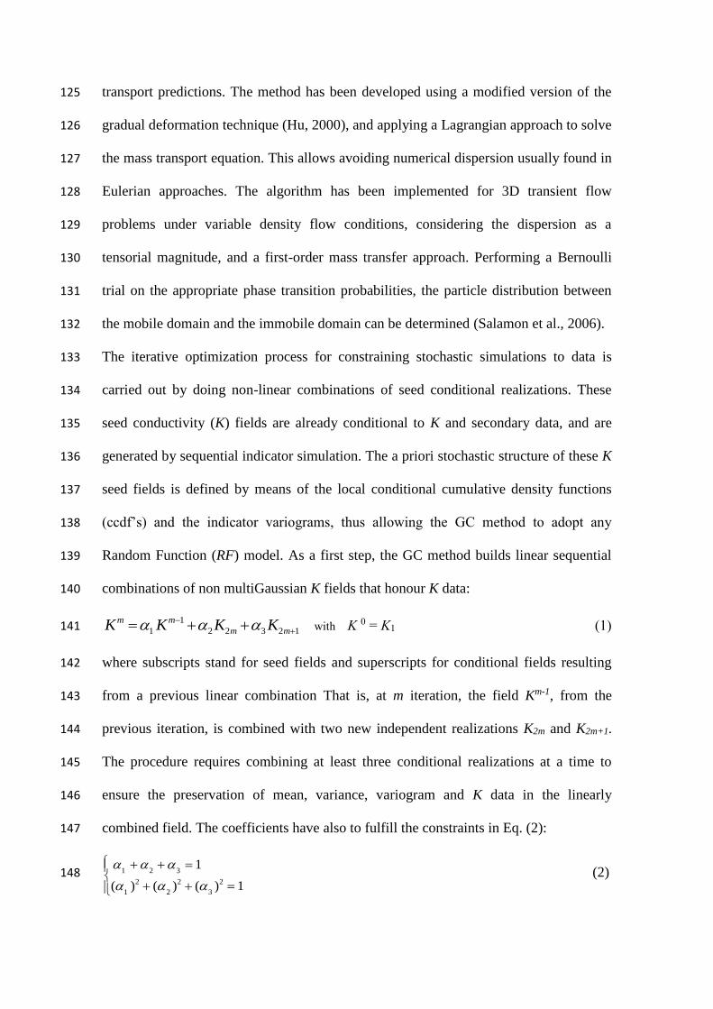
transport predictions. The method has been developed using a modified version of the 125

gradual deformation technique (Hu, 2000), and applying a Lagrangian approach to solve 126

the mass transport equation. This allows avoiding numerical dispersion usually found in 127

Eulerian approaches. The algorithm has been implemented for 3D transient flow 128

problems under variable density flow conditions, considering the dispersion as a 129

tensorial magnitude, and a first-order mass transfer approach. Performing a Bernoulli 130

trial on the appropriate phase transition probabilities, the particle distribution between 131

the mobile domain and the immobile domain can be determined (Salamon et al., 2006). 132

The iterative optimization process for constraining stochastic simulations to data is 133

carried out by doing non-linear combinations of seed conditional realizations. These 134

seed conductivity (K) fields are already conditional to K and secondary data, and are 135

generated by sequential indicator simulation. The a priori stochastic structure of these K 136

seed fields is defined by means of the local conditional cumulative density functions 137

(ccdf’s) and the indicator variograms, thus allowing the GC method to adopt any 138

Random Function (RF) model. As a first step, the GC method builds linear sequential 139

combinations of non multiGaussian K fields that honour K data: 140

1

1 2 2 3 2 1

m m

m mK K K K

with K 0 = K1 (1) 141

where subscripts stand for seed fields and superscripts for conditional fields resulting 142

from a previous linear combination That is, at m iteration, the field Km-1, from the 143

previous iteration, is combined with two new independent realizations K2m and K2m+1. 144

The procedure requires combining at least three conditional realizations at a time to 145

ensure the preservation of mean, variance, variogram and K data in the linearly 146

combined field. The coefficients have also to fulfill the constraints in Eq. (2): 147

1

2

3 1

(1)2 (

2)2 (

3)2 1

(2) 148

being the parameterization of 𝛼𝑖 given by Eq. (3): 149

1 1

3 2

3cos

2 1

3 2

3sin(

6) with [ ]

3 1

3 2

3sin(

6)

(3) 150

151

The 𝛼𝑖 coefficients are different in every iteration m, and correspond to a unique 152

parameter ; note the one to one correspondence between the parameter and the 153

combined realization Km. 154

Because the linear combination of independent non-Gaussian random functions does 155

not preserve the non-Gaussian distribution, although the variogram is preserved, a 156

transformation between Gaussian to the non-Gaussian fields (and vice versa) is 157

required. This transformation is performed through the probability fields (see Capilla 158

and Llopis-Albert 2009 for more details). Finally, at each iteration m of the method the 159

parameter is determined by minimizing an objective function that penalizes deviations 160

among computed and measured data. As aforementioned this way of operating has been 161

successfully applied in both synthetic and real cases. 162

The penalty function to be minimized is made up by the weighted sum of three terms: 163

𝑝𝑘(𝜃) = 𝑝ℎ𝑘(𝜃) + 𝑘𝑝𝑐

𝑘(𝜃) + 𝑘𝑝𝜏𝑘(𝜃) (4) 164

165

where 𝑝ℎ𝑘(𝜃) is the weighted sum of square differences between observed and 166

calculated values for piezometric heads, concentrations and travel times, respectively. 167

These terms are function of the parameter 𝜃, for every time step t and measurement 168

location i. The terms 𝑘 and 𝑘are trade-offs coefficients between the different 169

conditioning data (see Capilla and Llopis-Albert, 2009). 170

171

2.2. Hydro-economic model 172

The method is based on previous developments of the hydro-economic modeling 173

framework presented by Peña-Haro et al. (2009; 2011). The model was also applied to a 174

real-complex case study (Peña-Haro et al., 2010) and further extended to assess 175

different sources of uncertainty on the suggested control policies and the resulting 176

economic and environmental impacts (Llopis-Albert el al., 2014). 177

The stochastic optimization approach determines the spatial and temporal fertilizer 178

application rate that maximizes the net benefits in agriculture constrained by the quality 179

requirements in groundwater at various control sites. It quantifies the relationship 180

between emissions (fertilizer applied) and groundwater quality impacts or nitrate 181

concentration measured at regulatory control sites. The regulation of nitrate pollution is 182

examined within a cost-effectiveness way, in which the objective is to maximize the 183

sum of the net benefits from agricultural production while meeting the environmental 184

standards. The management model for groundwater pollution control is formulated as 185

follows, where the benefits in agriculture are determined by means of crop prices and 186

crop production functions: 187

, , ,

1

1s s s y n s y w s y s sy

s y

Max A p Y p N p W C Sr

(5) 188

subject to: 189

, , , , , ,c t s y s y c t

s

c t y RM cr q (6) 190

where is the objective function to be maximized and represents the present value of 191

the net benefit from agricultural production (€) defined as crop revenues minus fertilizer 192

and water variable costs; As is the area cultivated for crop located at source s; ps is the 193

crop price (€/kg); Ys,y is the production yield of crop located at source s at planning year 194

y (kg/ha), that depends on the nitrogen fertilizer and irrigation water applied; pn is the 195

nitrogen price (€/kg); Ns,y is the fertilizer applied to crop located at source s at year y 196

(kg/ha), pw is the price of water (€/m3), and Ws,y is the water applied to crop located at 197

source s at each planning year y (m3); Cs is the aggregation of the remaining per hectare 198

cost for crop located at source s (€/ha); Ss are the subsidies for the crop located at 199

source s (€/ha); r is the annual discount rate, RM is the unitary pollutant concentration 200

response matrix where each column is the nitrate concentration for each crop area (s) 201

times de number of years within the planning horizon (y), the number of rows equals the 202

number of control sites (c) times the number of simulated time steps (t) in the frame of 203

the problem; q is a vector of water quality standard imposed at the control sites over the 204

simulation time (kg/m3); cr is a vector representing the nitrate concentration recharge 205

(kg/m3) reaching groundwater from a crop located at source s, which is obtained 206

dividing the nitrate leached over the water that recharges the aquifer. Cs is the 207

aggregation of the remaining per hectare costs for crop located at sources (€/ha); Ss are 208

the subsidies for the crop located at source s (€/ha). 209

The response matrix (RM) describes the influence of pollutant sources upon 210

concentrations at the control sites over time. This is carried out by means of numerical 211

simulation models based on the flow and solute transport governing equations. 212

Specifically, in order to ensemble the pollutant response matrix we have used 213

MODFLOW (McDonald and Harbough, 1988), a 3D finite difference groundwater flow 214

model, and MT3DMS (Zheng and Wang, 1999), a 3D solute transport model. The 215

hydro-economic framework takes into account different processes governing nitrate in 216

groundwater in both the saturated and unsaturated zone of the aquifer. Then the 217

agronomic, and the flow and solute transport model consider processes ranging from 218

mineralization, nitrification, denitrification, volatization, immobilization, and plant 219

uptake in the unsaturated zone to advection, dispersion, diffusion and biodegradation in 220

the saturated zone. 221

The simulated time horizon corresponds to the time for the solute to pass all the control 222

sites, and it is independent of the length of the planning period. Once the field of 223

groundwater velocities is computed using the calibrated groundwater flow model, it is 224

used by the calibrated mass transport model to compute the nitrate concentrations over 225

time each control site (breakthrough curves) at resulting from unit nitrate concentration 226

recharges at each pollution source. These concentration values are assembled as 227

columns to conform the pollutant concentration RM, which is a rectangular (m x n) 228

matrix. The number of columns, n, equals the number of crop areas (pollution sources) 229

times the number of years within the planning horizon. The number of rows, m, equals 230

the number of control sites times the number of simulated time steps in the frame of the 231

problem. The integration of the response matrix in the constraints of the management 232

model allows simulating by superposition the evolution of groundwater nitrate 233

concentration over time at different points of interest throughout the aquifer resulting 234

from multiple pollutant sources distributed over time and space. The assumption of 235

linearity of the system is required in order to apply superposition. The advective and 236

dispersive transport depends on concentration and groundwater flow velocity. Because 237

concentration is unknown, the use of both velocity and concentration as decision 238

variables would create a non-linearity. As a result the underlying assumption is that the 239

irrigation rate at each source is not a decision variable and has a known influence upon 240

the velocity field. 241

Both nitrate leached and crop production are represented by polynomial regression 242

equations depending on the water and fertilizer use (Peña-Haro et al., 2009). These 243

equations are derived from the results of the agronomic simulation model GEPIC (Liu 244

et al., 2007), a GIS-based crop growth model integrating a bio-physical EPIC model 245

(Environmental Policy Integrated Climate) (Williams, 1995) with a GIS to simulate the 246

spatial and temporal dynamics of the major processes of the soil-crop-atmosphere-247

management systems. The GEPIC package simulates crop growth using local conditions 248

on climate, soil, irrigation water, tillage and other operations. The crop production 249

function was introduced into the management model as follows: 250

251

(7) 252

253

where Ys,y is the crop yield located at source s for a year y (kg/ha), Ws,y is the water 254

applied to the crop located at source s (m3/ha) and Ns,y is the fertilizer applied to the 255

crop located at source s (kg/ha) within the year y. The nitrogen leached is defined as 256

follows: 257

258

(8) 259

260

where Ls,y is the nitrogen leached (kg/ha), Ws,y is the water applied to the crop located at 261

source s (m3/ha) with in the year y, and Ns,y is the fertilizer applied to the crop located at 262

source s (kg/ha). 263

The non-linear optimization problem was coded in GAMS, a high-level modeling 264

system for mathematical programming problems (GAMS, 2012), while the solver used 265

was CONOPT (Drud, 1985). It is based on the Generalized Reduced Gradient algorithm 266

designed for large programming problems. 267

268

3. Application to a 2D synthetic case 269

ysysysysysysys NWfNeNdWcWbaY ,,

2

,,

2

,,,

ysysysysysysys NWlNkNjWiWhgL ,,

2

,,

2

,,,

A two-dimensional synthetic aquifer was selected to verify the methodology. It is based 270

on the configuration presented by Peña-Haro et al. (2009), which apply a deterministic 271

formulation to a 2D homogeneous synthetic aquifer. In this case, however, we consider 272

heterogeneous hydraulic conductivity. The aquifer has impermeable boundaries and 273

steady-state flow from top to bottom of the domain (Fig. 1). The aquifer domain was 274

divided in square cells of 500 x 500 m, with a grid made up of 58 rows and 40 columns. 275

A confined aquifer has been modeled with a saturated thickness of 10 m, effective 276

porosity of 0.2, and longitudinal dispersivity of 10 m. The natural annual recharge is 277

500 m3/ha. A temporal discretization of 70 stress periods was used, each of one-year 278

duration. In addition, seven different crop areas (which are the pollution sources in our 279

model formulation) with five different crops are considered. For each crop a quadratic 280

production function and a leaching function have been defined using Eq. (7) and (8). 281

The calibrated coefficients of those quadratic functions can be found in Peña-Haro et al. 282

(2009). The relationship between each source and the crop sown is depicted in Table 1, 283

which also shows the irrigation rates needed by each crop. A recovery time horizon of 284

the aquifer by the year 2015 is defined, which entails nitrate concentration lower than 285

50 mg/l for all control sites (three control wells are defined), as established by the EU 286

water legislation. 287

Two scenarios have been simulated in order to compare the groundwater nitrate 288

concentrations and net profits. In scenario 1 (S1) the fertilizer use is not constrained by 289

groundwater nitrate concentration standards at the control wells. It represents the 290

fertilizer application rates that return the maximum net benefits at each crop. 291

In scenario 2 (S2) the fertilizer used is constrained by the groundwater nitrate 292

concentration standards (50 mg/l) at the control wells. Finally, a planning horizon of 293

forty years was considered for each scenario with a constant annual fertilizer application 294

for the whole time period. 295

An ensemble of a hundred conditional seed K fields is generated by means of sequential 296

indicator simulation (SIS) by means of the code ISIM3D (Gómez-Hernández and 297

Srivastava, 1990). The conditional fields represent the Case 1 (C1). In addition, an 298

ensemble of unconditional K fields has also been generated in order to compare results 299

(Case 2, C2). This geostatistical tool allows controlling the bivariate (2-point) statistics 300

imposed on the simulated field instead of controlling a mere covariance model. As 301

aforementioned, these seed K fields are subsequently used by the inverse model to 302

constraint stochastic simulations to the available data. It should be mentioned that all 303

seed K fields honour the K data, while during the stochastic optimization procedure 304

carried out by the inverse model, the K fields are gradually modified to honour the flow 305

and mass transport data. Eighty-four K data were defined as conditioning data. They 306

have been selected to be homogeneously and spatially distributed over the whole aquifer 307

domain. Moreover, they differ in several orders of magnitude to obtain highly 308

heterogeneous aquifers. With the information provided by the K data we have defined 309

nine deciles of the cumulative distribution to give a reasonable discretization of the 310

local distribution and transformed to the corresponding indicator categories. The SIS 311

uses an indicator kriging (Deutsch and Journal, 1997) to build up a discrete conditional 312

cumulative density function (ccdf) for the individual categories at each case and the 313

node is assigned a category selected at random from this discrete ccdf. For a continuous 314

variable such as conductivity, indicator variables are built by comparing data values to a 315

set of thresholds, zk: 316

𝑖(𝐮𝛂; 𝑘) = {1 𝑖𝑓 𝑧(𝐮𝛂) ≤ 𝑧𝑘

0 𝑜𝑡ℎ𝑒𝑟𝑤𝑖𝑠𝑒} (9) 317

Spatial continuity for the different thresholds was then evaluated using the standardized 318

indicator semivariogram (e.g., Goovaerts, 1997): 319

𝛾𝐼(𝒉; 𝑧𝑘)

𝜎𝑖2

≈1

2𝑁(𝒉)𝒖1−𝒖2=𝒉±∆𝒉

∑[𝑖(𝒖1; 𝑧𝑘) − 𝑖(𝒖2; 𝑧𝑘)]2 (10) 320

321

where zk are the thresholds values; 𝜎𝑖2 is the indicator variance given as 𝜎𝑖

2 =322

𝐹(𝑧𝑘)[1 − 𝐹(𝑧𝑘)], and 𝐹(𝑧𝑘) is the marginal cumulative distribution function; N(h) is 323

the number of data pairs within the class of distance and direction; h is the separation 324

vector; z(u1,2) denotes a measurement with u1,2 being the vector of spatial coordinates of 325

the individual 1 or 2; and Δh is a tolerance vector. Finally, a mosaic variography was 326

chosen for the generation of the seed K fields with the defined spatial continuity. It is 327

spherical, with equal ranges in all directions of 40 m, 0.04 of nugget effect, and sill of 328

0.22. The generated seed fields are equally likely realizations, thus being plausible 329

representations of reality since they display the same degree of spatial variability. 330

Note that we have focused in order to generate the heterogeneous fields on the hydraulic 331

conductivity (K), since it is usually the parameter with the most significant spatial 332

variation. One of these seed K fields has been chosen to be the true K field (i.e., it 333

represents the actual heterogeneity in the aquifer). For the true field the hydraulic heads 334

(h) are obtained and used as conditioning data for the inverse model. The spatial 335

location of the 84 piezometric head data is the same than those defined for the K data. 336

The a priori conditional cumulative density function (ccdf) have been defined 337

displaying a highly asymmetrical distribution with a long lower tail; thus assigning 338

higher probabilities of occurrence to high K values (i.e., it could represent fracture 339

structures). This is how the GC method allows integrating the available hard data and 340

also the geological information. Note that GC method honors the a priori ccdf’s during 341

the whole conditioning process, while other inverse modeling techniques deal with 342

secondary information incorporating it in initially generated fields to be perturbed, not 343

having any implemented constraint to keep honoring these data. Furthermore, GC 344

method tends to preserve the local ccdf’s during the whole perturbation process of seed 345

K fields to obtain conditional simulations see Llopis-Albert and Capilla (2009). This 346

means that if there are zones with ccdf’s belonging to independent stochastic processes 347

they are still preserved. In addition, conductivities can vary, due to the deformation 348

process, several orders of magnitude, and because of how the non-Gaussian feature is 349

introduced in the inverse model by means of the probability fields allows the 350

reproduction of strings of extreme values of K or preferential flow paths (Llopis-Albert 351

and Capilla, 2009). Moreover, as many authors have pointed out (e.g., Gómez-352

Hernández and Wen, 1998), preferential flow pathways may play a crucial role for 353

tracer transport and may reflect some geological settings, e.g., channelling. 354

Eventually, for each one of the calibrated K fields obtained with the inverse model the 355

pollutant concentration response matrix is calculated, and the hydro-economic model 356

run. 357

358

4. Results and discussion 359

Fig. 3 shows the Cumulative Density Functions (CFD’s) of the maximum benefits 360

obtained in the aquifer for both groundwater quality scenarios (S1 and S2) and both 361

conditional (to K and h data) and unconditional conductivity realizations (i.e., cases C1 362

and C2). Note that a forty year planning period is considered and a recovery time 363

horizon for the aquifer by the year 2015 has been defined, as established by the WFD. 364

As logical, this figure shows that when no groundwater quality restrictions are applied 365

in the optimization management model (i.e., for scenario S1) the same benefit is 366

obtained for all realizations and both cases, i.e., conditional and unconditional K fields. 367

Moreover, it represents the maximum benefit that can be achieved in the aquifer with 368

the defined set of parameters and variables. This is because farmers can applied as much 369

as fertilizer as required by each crop to maximize their yields as defined in Eq. (7). 370

Then, for scenario S1, the maximum benefit takes the value of 21.06 M€/year for all 371

realizations and both cases, so that the standard deviations of such CDF’s are zero. 372

Contrary, for scenario S2, when groundwater quality constraints are applied (i.e., 373

maximum nitrate concentrations of 50 mg/l are allowed at control wells) the benefits are 374

reduced for all realizations and both cases. As expected, for conditional K fields (C1) 375

and scenario S2, the uncertainty in the maximum benefits achieved in the aquifer is 376

strongly reduced if compared with the unconditional realizations (C2). In fact, the CDF 377

of the maximum benefits has a mean of 20.91 M€/year and a standard deviation of 378

0.074 M€/year for case C1, while it has a mean of 20.79 M€/year and a standard 379

deviation of 0.22 M€/year for case C2. This proves the worth of the methodology to 380

provide more reliable policies since it reduces the hydrogeological parameter 381

uncertainty, and therefore, the uncertainty in the decision variables of the management 382

model. 383

Similar results are obtained for the fertilizer applied to the aquifer as shown in Fig. 3. It 384

depicts the Cumulative Density Functions (CFD’s) of the total fertilizer applied to the 385

aquifer for both groundwater quality scenarios and both conditional and unconditional 386

conductivity fields. Then, the maximum fertilizer applied to the aquifer is obtained for 387

S1. It has for both cases a mean of 3741.3 (ton/year) and a standard deviation of zero 388

For S2, case C1 has a mean of 3502.03 (ton/year) and a standard deviation of 129.51 389

(ton/year), while C2 takes the values of 3546.34 and 57.01, respectively. Again, there is 390

an important reduction in the uncertainty of the fertilizer applied to the aquifer. 391

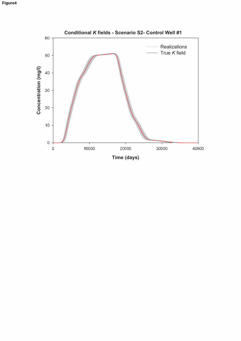
Furthermore, the reduction of uncertainty is also depicted in Fig. 4, which shows the 392

breakthrough curves for control well #1 and scenario S2 (with groundwater quality 393

constraints of 50 mg/l) of all conditional conductivity realizations (C1). This figure 394

shows how close are the time series of nitrate concentrations of all conditional 395

realizations to the true K field. Note that these concentrations are restricted by the 396

management model to be lower, during the whole planning period, than the standard 397

enacted by the WFD. 398

The trade-offs between the economic returns and the reliability in meeting the 399

environmental standards can be compared for both scenarios. Fig. 2 and 3 show how the 400

scenario S1 leads to higher benefits that the scenario S2. Then higher nitrate 401

concentrations in the aquifer lead to lower benefits and vice versa. Therefore, these 402

trade-offs have been quantified under the WFD standards. Furthermore, they have been 403

quantified under an uncertain environment by means of the CDF of the agricultural 404

benefits and their respective nitrate concentrations. 405

406

5. Conclusions 407

In recent years, the concern about nitrate concentrations in groundwater has increased 408

on account of the intensive use of fertilizers in agriculture. Water legislations have dealt 409

with such issue by establishing limits of nitrate concentrations in groundwater bodies. In 410

Europe, the EU WFD establishes limits of 50 mg/l, and requires that groundwater 411

bodies reach a good quantitative and chemical status by 2015. Then to control 412

groundwater diffuse pollution is necessary to analyze and implement complex 413

management decisions. However, the decision-making process is even more complex 414

under uncertain environments and heterogeneous stakeholder’s interests. This 415

uncertainty leads to different management policies with clear implications in reliability 416

levels, costs and benefits. Therefore policy-makers need agricultural advice services to 417

help them to come up with the best management practices. Such advices can be derived 418

from the results provided by the tool here presented, which entails the coupling of a 419

stochastic inverse model with a hydro-economic model. This allows reducing 420

uncertainty by constraining stochastic simulations to data. The stochastic hydro-421

economic modeling framework has been verified in a 2D synthetic aquifer and its worth 422

for agricultural advice services demonstrated. It has been proved to be a valuable tool in 423

estimating non-Gaussian hydrogeological parameters such as the hydraulic conductivity 424

in highly heterogeneous aquifers. This leads to reducing uncertainty in concentration 425

distributions of contaminant plumes at control wells when reasonable amount of data is 426

available. Finally, this is translated into a reduction of the uncertainty on the results of 427

the hydro-economic model: maximum benefits, optimal strategies of spatial and 428

temporal allocation of fertilizer use in agriculture and concentrations in the aquifer that 429

meet certain groundwater quality standards. This has been carried out by means of a 430

sensitivity analyses for conditional and unconditional K fields. Furthermore, the trade-431

offs between higher economic returns and reliability in meeting the environmental 432

standards have been analyzed for different groundwater quality scenarios. The study of 433

the least-cost alternative for meeting the environmental objectives is also important in 434

order to justify potential time and objective derogation when disproportionate costs are 435

identified (WFD, art. 4). 436

As a further research we could have considered different groundwater quality standards, 437

recovery time horizons, different spatial structure of the conductivity fields, or different 438

sets of flow and mass transport conditioning data (for instance, regarding the spatial 439

location and/or temporal). 440

441

442

References 443

- Bakr, M.I., te Stroet, C.B.M., Meijerink, A., 2003. Stochastic groundwater quality management: Role of 444

spatial variability and conditioning, Water Resour. Res., 39(4), 1078, doi:10.1029/2002WR001745. 445

- Capilla, J.E., Llopis-Albert, C., 2009. Stochastic inverse modeling of non multiGaussian transmissivity 446

fields conditional to flow, mass transport and secondary data. 1 Theory. Journal of Hydrology, 371, 66-447

74. doi:10.1016/j.jhydrol.2009.03.015. 448

- Deutsch, C.V., Journal, A.G., 1997. GSLIB: Geostatistical Software Library and User's GUide. New 449

York, Oxford University Press. 450

- Drud, A., 1985. CONOPT: a GRG code for large sparse dynamic nonlinear optimization problems. 451

Math. Program. 31, 153e191. doi:10.1007/BF02591747. 452

- EC, 1980. Council Directive 80/778/EEC relating to the quality of water intended for human 453

consumption. Official Journal of the European Communities, L229 (30.08.1980), pp. 11-29. 454

- EC, 2000. Directive 2000/60/EC of the European Parliament and of the Council of October 23 2000 455

Establishing a Framework for Community Action n the Field of Water Policy. Official Journal of the 456

European Communities, L327/1eL327/72. 22.12.2000. 457

- Gómez-Hernández, J.J., Srivastava, R.M., 1990. ISIM3D: An ANSI-C three dimensional multiple 458

indicator conditional simulation program. Computer and Geosciences, 16(4), 395-440. 459

- Gómez-Hernández, J.J., Wen, X.H., 1998. To be or not to be multiGaussian? A reflection on stochastic 460

hydrogeology. Advances in Water Resources 21 (1), 47–61. 461

- Hu, L.Y., 2000. Gradual deformation and iterative calibration of gaussian-related stochastic models. 462

Mathematical Geology, Vol. 32, No 1, 2000, 87-108. 463

- Neupauer, R.M., Wilson, J.L., 1999. Adjoint method for obtaining backward-in-time location and travel 464

time probabilities of a conservative groundwater contaminant. Water Resources Research, 35(11), 3389-465

3398. 466

- Llopis-Albert, C., 2008. Stochastic inverse modelling in non-multiGaussian media conditional to flow, 467

mass transport and secondary data. PhD Thesis, Universitat Politècnica de València, 274 pp. ISBN: 978-468

84-691-9796-7. 469

- Llopis-Albert, C., Capilla, J.E., 2009. Stochastic inverse modeling of non multiGaussian transmissivity 470

fields conditional to flow, mass transport and secondary data. 2 Demonstration on a synthetic aquifer. 471

Journal of Hydrology, 371, 53–65. doi:10.1016/j.jhydrol.2009.03.014. 472

- Llopis-Albert, C., Capilla, J.E., 2009a. Gradual conditioning of non-Gaussian transmissivity fields to 473

flow and mass transport data: 3. Application to the Macrodispersion Experiment(MADE-2) site, on 474

Columbus Air Force Base in Mississippi (USA). Journal of Hydrology 371, 75–84. 475

doi:10.1016/j.jhydrol.2009.03.016. 476

- Llopis-Albert, C., Capilla, J.E., 2010. Stochastic simulation of non-Gaussian 3D conductivity fields in a 477

fractured medium with multiple statistical populations: case study. Journal of Hydrologic Engineering, 478

15, 554-566. doi: 10.1061/(ASCE)HE.1943-5584.0000214. 479

- Llopis-Albert, C., Capilla, J.E., 2010a. Stochastic inverse modelling of hydraulic conductivity fields 480

taking into account independent stochastic structures: A 3D case study. Journal of Hydrology 391, 277–481

288. doi:10.1016/j.jhydrol.2010.07.028. 482

- Llopis-Albert, C., Pulido-Velazquez, M., Peña-Haro, S., 2014. Assessment of the effect of uncertainty 483

on groundwater nitrate pollution control from agriculture. Environmental Modelling & Software, 484

submitted. 485

- McDonald, M.G., Harbough, A.W., 1988. A Modular Three-Dimensional Finite-Difference 486

Groundwater Flow Model, US Geological Survey Technical Manual of Water Resources Investigation, 487

Book 6, US Geological Survey, Reston, Va, 586 p. 488

- Peña-Haro S., Pulido-Velazquez, M., Sahuquillo, A., 2009. A hydro-economic modeling framework for 489

optimal management of groundwater nitrate pollution from agriculture. Journal of Hydrology, 373, 193–490

203, doi:10.1016/j.jhydrol.2009.04.024. 491

- Peña-Haro, S., Llopis-Albert, C., Pulido-Velazquez, M, Pulido-Velazquez, D., 2010. Fertilizer standards 492

for controlling groundwater nitrate pollution from agriculture: El Salobral-Los Llanos case study, Spain. 493

Journal of Hydrology, 392, 174–187. 494

- Peña-Haro, S., Pulido-Velazquez, M., Llopis-Albert C., 2011. Stochastic hydro-economic modeling for 495

optimal management of agricultural groundwater nitrate pollution under hydraulic conductivity 496

uncertainty. Environmental Modelling & Software 26, 999-1008. 497

- Poeter, E.P., Hill, M.C., 1997. Inverse models: a necessary next step in ground-water modeling. Ground 498

Water;35(2):250–60. 499

- Rehfeldt, K.R., Boggs, J.M., Gelhar, L.W., 1992. Field study of dispersion in a heterogeneous aquifer 3. 500

Geostatistical analysis of hydraulic conductivity. Water Resources Research, 28(12), 3309–3324. 501

- Renard, P., 2007. Stochastic hydrogeology: what professionals really need? Ground Water, 45(5):531–502

41. doi:10.1111/j.1745-6584.2007.00340.x. 503

- Salamon P., Fernàndez-Garcia, D., Gómez-Hernández, J.J., 2006. Modeling mass transfer processes 504

using random walk particle tracking. Water Resources Research, 42, W11417, 505

doi:10.1029/2006WR004927. 506

- Smith, L., Schwartz, F.W., 1981. Mass transport, 2. Analysis of uncertainty in prediction. Water 507

Resources Research, 17(2):351–69. 508

- Williams, J.R., 1995. The EPIC model. In: Singh, V.P. (Ed.) Computer Models of Watershed 509

Hydrology, 909-1000. Water Resources Publisher. 510

- Zheng, C., Wang, P., 1999. MT3DMS: A Modular Three-Dimensional Multispecies Transport Model 511

for Simulation of Advection, Dispertion and Chemical Reactions of Contaminants in Groundwater 512

Systems; Documentation and User`s Guide. 513

514

515

516

517

518

519

520

521

522

523

524

525

Table 1. Sources, crops and irrigation. 526

527

Source Crop Area (ha) Water applied (m3/ha) Crop price (€/kg)

S1 Alfalfa 3600 950 0.09

S2 Barley 3600 300 0.12

S3 Sunflower 3600 400 0.30

S4 Wheat 3600 250 0.13

S5 Corn 3600 700 0.12

528

529

City

LakeConstant Head

I mpermeabl e I mpermeabl e

Control Site 2 Control Site 3Control Site 1

29k m

20 km

Cells: 500 x 500 mConstant HeadFigure1

Figure2

Figure3

0 10000 20000 30000 400000102030405060

Figure4

Figure Captions

Figure 1. Problem domain, boundary conditions, control areas (si) and crops and spatial

location of the observation sites.

Figure 2. Cumulative Density Functions (CFD’s) of the maximum benefits (M€/year)

for both groundwater quality scenarios and both conditional and unconditional

conductivity fields.

Figure 3. Cumulative Density Functions (CFD’s) of the total fertilizer applied to the

aquifer (Ton/year) for both groundwater quality scenarios and both conditional and

unconditional conductivity fields.

Figure 4. Breakthrough curves for control well #1 and scenario S2 (groundwater quality

constraints of 50 mg/l) of the conditional conductivity fields. The figure also shows the

true field. A planning period of forty years is considered.

Figure captions