Document de Recherche du Laboratoire d’Économie d’Orléans

DR LEO 2015-13

Immigration and Economic Growth in the OECD Countries 1986-2006

Ekrame BOUBTANE Jean-Christophe DUMONT

Christophe RAULT

Laboratoire d’Économie d’Orléans Collegium DEG

Rue de Blois - BP 26739 45067 Orléans Cedex 2

Tél. : (33) (0)2 38 41 70 37 e-mail : leo@univ-orleans.fr

www.leo-univ-orleans.fr/

Immigration et croissance économique dans les pays de l'OCDE sur la période 1986-2006

Immigration and economic growth in the OECD countries 1986-

20061

Ekrame Boubtane CERDI-University of Auvergne, and CES-University of Paris 1

E-mail: ekrame.boubtane@gmail.com

Jean-Christophe Dumont International Migration Division (OECD)

E-mail: Jean-Christophe.Dumont@oecd.org

Christophe Rault University of Orléans, CNRS, LEO, UMR 7322, F45067, Orléans, France

E-mail: chrault@hotmail.com, website: http://chrault3.free.fr/ (Corresponding Author)

Résumé: Ce papier reconsidère l'impact des migrations internationales sur la croissance économique pour 22 pays de OCDE entre 1986-2006 et repose sur une base de données originale que nous avons compilée, qui permet de distinguer entre le solde migratoire des autochtones et des étrangers, par niveau de qualification. Plus précisément, après avoir introduit les flux migratoires dans un modèle de Solow-Swan augmenté, nous estimons un modèle dynamique sur données de panel par la méthode des moments généralisés (SYS-GMM) afin de tenir compte de l'endogénéité potentielle de la variable migration. Deux conclusions importantes ressortent de notre analyse. Premièrement, il existe un impact positif du capital humain des migrants sur le PIB par tête, et deuxièmement, une hausse permanente des flux migratoires exerce un effet positif sur la croissance de la productivité. Cependant, l'impact de l'immigration sur la croissance demeure faible, et cela, même dans les pays ayant des politiques migratoires sélectives. Mots clés: Immigration, Croissance, Capital Humain, Méthode des moments généralisés. Classification JEL: C23, F22, J24, J61, O41, O47.

Abstract: This paper offers a reappraisal of the impact of migration on economic growth for 22 OECD countries between 1986--2006 and relies on a unique data set we compiled that allows us to distinguish net migration of the native- and foreign-born populations by skill level. Specifically, after introducing migration in an augmented Solow-Swan model, we estimate a dynamic panel model using a system of generalized method of moments (SYS-GMM) to address the risk of endogeneity bias in the migration variables. Two important findings emerge from our analysis. First, there exists a positive impact of migrants' human capital on GDP per capita, and second, a permanent increase in migration flows has a positive effect on productivity growth. However, the growth impact of immigration is small even in countries that have highly selective migration policies. Keywords: Immigration, Growth, Human capital, Generalized Methods of Moments. JEL Classification: C23, F22, J24, J61, O41, O47. 

                                                            1 We would like to thank Fréderic Docquier, Raquel Carrasco, John Martin, Stefano Scarpetta, Gilles Spielvogel, and Bertrand Wigniolle for discussion and helpful comments on earlier drafts. This work was supported by the Agence Nationale de la Recherche of the French government through the Investissements d'avenir (ANR-10-LABX-14-01) programme.The usual disclaimer applies. 

1 Introduction

International migration to OECD countries, notably labour migration, has increasedsignificantly over the past decades. Between 1997 and 2007, in most southern Euro-pean countries, the United Kingdom, the United States, and several Nordic countries,immigrants contributed to more than 40% of net job creation. In 2007, the share ofimmigrants in employment reached 12% on average in OECD countries (OECD, 2009).In many developed countries, the first effects of population ageing can already be feltwithin the working age population as baby boomers begin to retire in large numberswhile younger cohorts are still too few to replace them. In this context, labour migra-tion will continue to play a significant role over the medium and long term. Specifically,international migration is expected to account for all labour force growth between 2005and 2020 in the OECD area as a whole.

At the same time, many countries have recently adapted their migration systemsto make them more selective vis-a-vis skills and education. The traditional settlementcountries (Australia, Canada, New Zealand, and the United States) have relied onskills-based migration programmes for a long time, which now serve as models to othercountries. The United Kingdom, Denmark, and the Netherlands have recently insti-tuted reforms to prioritize highly educated migrants through a points-based migrationsystem. Furthermore, the European Union has adopted a new directive, the EuropeanBlue Card, to attract highly qualified migrants to the European labour market. Thisdirective does not prevent EU Member States from maintaining their own systems ofnational residence permits for highly skilled migrants, but such national permits cannotgrant the right of residence in other EU Member States as is guaranteed under the BlueCard Directive. Accordingly, most European countries have also implemented specificmigration programmes to attract highly skilled foreign workers. For instance, Austriaadopted a points-based immigration scheme, the Red-White-Red Card, in July 2011.This system aims to attract highly qualified persons and skilled workers in shortageoccupations who wish to settle, with their families, permanently in Austria. Addition-ally, the United Kingdom changed its points system in 2011 to increase selectivity. Thehighly skilled migrant programme has been replaced by an ‘Exceptional Talent’ visafor applicants who are ‘internationally recognised leaders or emerging leaders’ in theirfields. This trend is likely to continue, and may even be reinforced, in the future.

These changes in migration trends and policies prompted us to reconsider the eco-nomic impact of migration. Empirical economic analyses have been flourishing in re-cent years in two key areas that are likely to influence public opinion on migration,namely, the labour market (Borjas, 2003; Angrist and Kugler, 2003; Lubotsky, 2007)and the fiscal effects of immigration (Auerbach and Oreopoulos, 1999; Storesletten,2000; Rowthorn, 2008). However, debate is relatively quiet regarding a third majorarea of interest: the impact of migration on economic growth. This is precisely thequestion addressed by this paper.

Although there are few doubts about the impact of a labour shock due to migration

2

on aggregate GDP, the effect is less obvious with regard to per capita GDP. Indeed, inthe standard augmented neoclassical growth model developed by Mankiw et al. (1992),a permanent increase in migration flows has a negative impact on long-term GDP percapita because of capital dilution, which might be compensated by a positive contribu-tion of new migrants to human capital accumulation (Dolado et al., 1994 ; Barro andSala-i-Martin, 1995). Consequently, in this framework, whether migration positively af-fects per capita GDP crucially depends on the scope of migration and its demographicand educational structures.

Due to a lack of harmonized international data on migration, few empirical stud-ies have attempted to estimate the impact of permanent immigrant flows on economicgrowth while accounting for educational attainment. The most closely related paperis Dolado et al. (1994). They estimate –as we do herein– a structural model includingimmigrants’ human capital. However, they do not observe migrants’ education, so theyuse the educational attainment of the population in the country of origin as a proxy.Moreover, their analysis covers the period from 1960–1985, which was characterized(until the second oil shock at the end of the 1970s) by low-skilled migration concen-trated in the manufacturing sector. Over the past two decades, the characteristics ofinternational migration have evolved considerably, and its impact must therefore to bereconsidered. That is the purpose of this paper.

This paper is also related to recent studies that analyse the effects of economic open-ness and diversity on GDP per capita. For example, Felbermayr et al. (2010) estimatethe effect of the stock of migrants on per capita income using cross-sectional countrydata. Andersen and Dalgaard (2011) consider temporary cross-border flows of people asa measure of global integration and evaluate the effect of the intensity of travel on GDPper capita. Ortega and Peri (2014) estimate the effect of economic openness by jointlyconsidering migration and trade on income per person. In line with studies on birth-place diversity and economic development, they take into account diversity by countryof origin within the stock of immigrants. Alesina et al. (2013) estimate the effect ofdiversity in migrant birthplaces on growth. They build diversity indicators from dataon immigration population by country of birth and education.

This paper departs from existing studies by considering the effect of permanentflows of immigrants by country of birth and skill level on GDP per capita. We focus onpermanent migration –movements that the receiving country considers to be long term.We exclude temporary visitors (i.e., for tourism and business purposes) because we aremainly interested in the economic consequences of long-term immigrants. Moreover, wefocus on newly arrived immigrants rather than the immigrant population as a whole.Indeed, the socioeconomic characteristics of immigrants have changed over time andflows reflect these changes better than the stock of immigrants. We also independentlyidentify the effect of net migration of the foreign- and native-born by skill level.

Specifically, we contribute to the existing literature in two ways. First, we compile

3

a unique data set on net migration that includes data on country of birth and skill levelfrom various data sources for 22 OECD countries for 1986–2006. Moreover, specific at-tention is devoted to producing robust measures of the educational attainment of recentimmigrants as well as of native-born expatriates who return to their home countries.Second, our estimations are based on the system of generalized method of moments(SYS-GMM) for dynamic panel data models developed by Arellano and Bover (1995)and Blundell and Bond (1998), which address the (potential) endogeneity of migrationvariables. However, the consistency of the SYS-GMM crucially depends on the validityof the instruments used. Therefore, in contrast to previous studies, we carefully followsome of the recommendations of Roodman (2009) and Bazzi and Clement (2013), in-troducing both internal and external instruments in our estimation. We consider thismethod to be a useful complement to standard specification tests for obtaining validinstruments and robust econometric results.

Our econometric investigation provides evidence that, over the period considered,the impacts of a permanent increase in net migration on GDP per capita via humancapital accumulation and capital dilution are significant and with the expected signs(i.e., positive and negative, respectively). Furthermore, simulations based on these re-sults indicate that the former dominates the latter, in almost all OECD countries. Thus,all else being equal, an increase of one percentage-point in foreign-born net migrationwould increase productivity growth by an average of three-tenths of a percentage-pointper year for the 22 OECD countries considered. Therefore, migration flows tend to havea positive but small impact on transitional productivity growth, even in countries thathave highly selective migration policies.

The remainder of the paper is organised as follows. Section 2 provides a short reviewof the literature. Section 3 outlines the theoretical model. Section 4 describes theeconometric strategy, data and empirical results. Section 5 discusses the implications ofthe results. Finally, Section 6 offers some concluding remarks. Technical details of thetheoretical model and, data sources and descriptions are contained in the Appendix.

2 Direct and indirect effects of migration on economicgrowth: an overview of the literature

International migration potentially has both direct and indirect effects on economicgrowth. First, migration can be viewed as a demographic shock. Indeed, in the text-book Solow-Swan growth model, an increase in migration has a negative impact onthe transitional path to the long-term steady state, in which all per capita variables arenonetheless stable. Even in this framework, however, migration affects the age structureof the destination country population because migrants tend to be more concentratedin active age groups compared to natives. Consequently, migration reduces dependencyratios and potentially has a positive impact on aggregate savings,1 which may eventuallyresult in higher total factor productivity (TFP) growth. Yet, this transmission channel

1This effect may be partially offset by remittances sent by migrants to their country of origin.

4

has not been directly considered in the literature.Second, migrants arrive with skills and abilities, that supplement the stock of humancapital in the host country. To our knowledge, Dolado et al. (1994) were the first tointroduce migration into the Solow-Swan model augmented by human capital. In thisframework, the contribution of immigrants to human capital accumulation compensates(at least partially) for the negative capital dilution effect associated with populationgrowth. The authors estimate their model for 23 OECD countries between 1960 and1985.

More recently, several authors have included migration in endogenous economicgrowth models. This literature considers the impact of immigrants on technologicalprogress, notably, their contributions to innovation.2 Walz (1995), for instance, intro-duces migration in a two country endogenous growth model. He finds that the sign ofthe growth rate effect depends on the initial specialization of the two countries and thatmigration is selective towards high-skilled individuals. Robertson (2002) also analysesthe impact of migration in an Uzawa-Lucas model with unskilled labour and shows thatan inflow of relatively unskilled immigrants results in lower transitional growth.Lundborg and Segerstrom (2000, 2002) include migration in a quality ladders growthmodel. They find that free migration stimulates growth, especially if it responds to dif-ferences in labour force endowments. Similarly, in an expansion-in-varieties framework,Bretschger (2001) shows that skilled migration can promote growth by decreasing thecosts of research and development and by increasing the market share of certain typesof goods.

Most of the previous studies are theoretical, and there exist very few empirical as-sessments of the impact of migration on economic growth. Furthermore, when suchanalyses exist, they are not based on structural models and are often hampered bydata constraints. For instance, Ortega and Peri (2009) analyse the effects of immigra-tion flows on total employment, physical capital accumulation and TFP in 14 OECDcountries between 1980 and 2005. They find that migration increases employment andcapital stocks but does not have a significant effect on TFP. Because immigration shockslead to an increase in total employment and a proportional response in production, out-put per capita is not affected by inflows of migrants. However, this study does not takeinto account the human capital of migrants, or diversity in their country of origin. Morerecently, Felbermayr et al. (2010) and Ortega and Peri (2014) use bilateral migrationstocks around the year 2000 to estimate a positive relationship between the immigrantshare of the population and GDP per capita in the host country. Moreover, Ortegaand Peri (2014) find that this positive relationship is magnified when diversity in thecountry of origin within the immigrant population is taken into account. These resultsare in line with the findings from studies on birthplace diversity and economic develop-ment. For example, Alesina et al. (2013) find a positive effect of immigrant populationdiversity in country of birth and education on growth.

2Hunt and Gauthier-Loiselle (2010) provide evidence on the impact of highly skilled migration in theUnited States on innovation. They find that a one percentage-point increase in the share of immigrantcollege graduates in the population increases patents per capita by 6%.

5

Another approach is to use time-series analysis. Morley (2006), for instance, anal-yses the causality between migration and economic growth using data for Australia,Canada, and the United States between 1930 and 2002. He finds evidence of long-runcausality running from per capita GDP to immigration but not the reverse. In anotherexample, Boubtane et al. (2013) find a positive bidirectional relationship between im-migration and GDP per capita for 22 OECD countries from 1987–2009. Note that dueto the lack of harmonized data on characteristics of migration flows, time-series studiesdo not take into account the educational attainment of immigrants.

The main contribution of this paper is to provide robust estimates of the impact ofnet migration flows on GDP per capita, controlling for the skill composition of recentimmigrants, using a clear theoretical framework. This framework is presented in thenext section.

3 The theoretical model

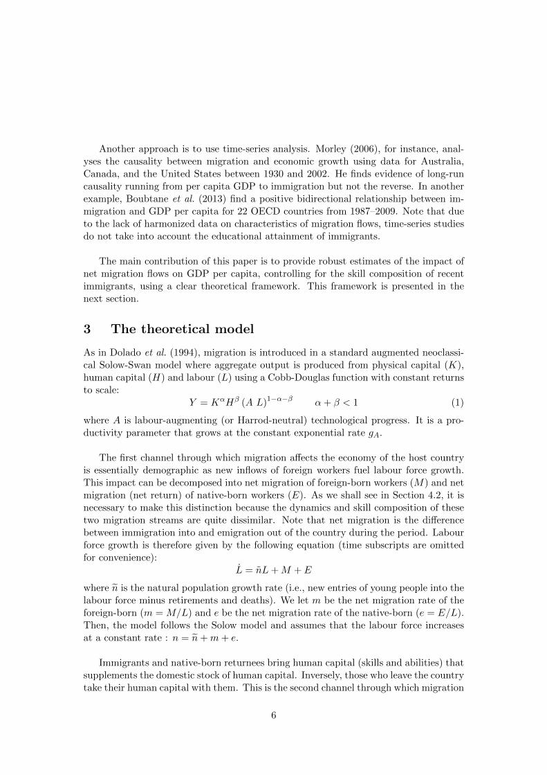
As in Dolado et al. (1994), migration is introduced in a standard augmented neoclassi-cal Solow-Swan model where aggregate output is produced from physical capital (K),human capital (H) and labour (L) using a Cobb-Douglas function with constant returnsto scale:

Y = KαHβ (A L)1−α−β α+ β < 1 (1)

where A is labour-augmenting (or Harrod-neutral) technological progress. It is a pro-ductivity parameter that grows at the constant exponential rate gA.

The first channel through which migration affects the economy of the host countryis essentially demographic as new inflows of foreign workers fuel labour force growth.This impact can be decomposed into net migration of foreign-born workers (M) and netmigration (net return) of native-born workers (E). As we shall see in Section 4.2, it isnecessary to make this distinction because the dynamics and skill composition of thesetwo migration streams are quite dissimilar. Note that net migration is the differencebetween immigration into and emigration out of the country during the period. Labourforce growth is therefore given by the following equation (time subscripts are omittedfor convenience):

L = nL+M + E

where n is the natural population growth rate (i.e., new entries of young people into thelabour force minus retirements and deaths). We let m be the net migration rate of theforeign-born (m = M/L) and e be the net migration rate of the native-born (e = E/L).Then, the model follows the Solow model and assumes that the labour force increasesat a constant rate : n = n+m+ e.

Immigrants and native-born returnees bring human capital (skills and abilities) thatsupplements the domestic stock of human capital. Inversely, those who leave the countrytake their human capital with them. This is the second channel through which migration

6

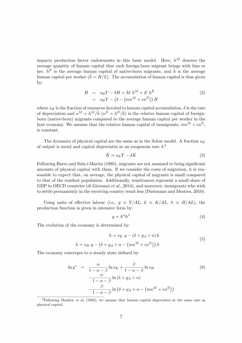
impacts production factor endowments in this basic model. Here, hM denotes theaverage quantity of human capital that each foreign-born migrant brings with him orher, hE is the average human capital of native-born migrants, and h is the averagehuman capital per worker (h = H/L). The accumulation of human capital is thus givenby:

·H = sHY − δH +M hM + E hE (2)

= sHY −(δ −

(mκM + eκE

))H

where sH is the fraction of resources devoted to human capital accumulation, δ is the rateof depreciation and κM = hM/h (κE = hE/h) is the relative human capital of foreign-born (native-born) migrants compared to the average human capital per worker in thehost economy. We assume that the relative human capital of immigrants, mκM + eκE ,is constant.

The dynamics of physical capital are the same as in the Solow model. A fraction sKof output is saved and capital depreciates at an exogenous rate δ:3

K = sKY − δK (3)

Following Barro and Sala-i-Martin (1995), migrants are not assumed to bring significantamounts of physical capital with them. If we consider the costs of migration, it is rea-sonable to expect that, on average, the physical capital of migrants is small comparedto that of the resident population. Additionally, remittances represent a small share ofGDP in OECD countries (di Giovanni et al., 2014), and moreover, immigrants who wishto settle permanently in the receiving country remit less (Dustmann and Mestres, 2010).

Using units of effective labour (i.e., y ≡ Y/AL, k ≡ K/AL, h ≡ H/AL), theproduction function is given in intensive form by:

y = kαhβ (4)

The evolution of the economy is determined by:

·k = sK y − (δ + gA + n) k

·h = sH y −

(δ + gA + n−

(mκM + eκE

))h

(5)

The economy converges to a steady state defined by:

ln y∗ =α

1− α− βln sK +

β

1− α− βln sH (6)

− α

1− α− βln (δ + gA + n)

− β

1− α− βln(δ + gA + n−

(mκM + eκE

))3Following Mankiw et al. (1992), we assume that human capital depreciates at the same rate as

physical capital.

7

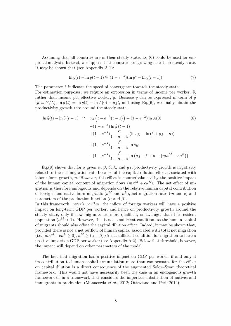
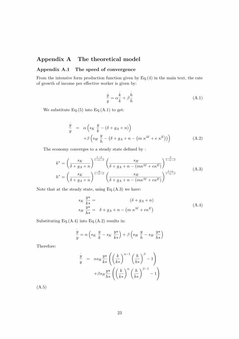
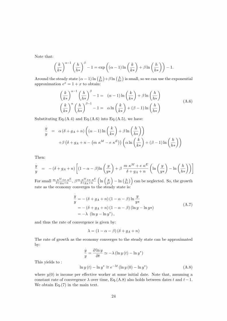
Assuming that all countries are in their steady state, Eq.(6) could be used for em-pirical analysis. Instead, we suppose that countries are growing near their steady state.It may be shown that (see Appendix A.1):

ln y(t)− ln y(t− 1) ∼= (1− e−λ)(ln y∗ − ln y(t− 1)) (7)

The parameter λ indicates the speed of convergence towards the steady state.For estimation purposes, we require an expression in terms of income per worker, y,rather than income per effective worker, y. Because y can be expressed in term of y(y ≡ Y/L), ln y (t) = ln y(t) − lnA(0) − gAt, and using Eq.(6), we finally obtain theproductivity growth rate around the steady state:

ln y(t)− ln y (t− 1) ∼= gA

(t− e−λ(t− 1)

)+ (1− e−λ) lnA(0) (8)

−(1− e−λ) ln y (t− 1)

+(1− e−λ)α

1− α− β(ln sK − ln (δ + gA + n))

+(1− e−λ)β

1− α− βln sH

−(1− e−λ)β

1− α− βln(gA + δ + n−

(mκM + eκE

))Eq.(8) shows that for a given α, β, δ, λ, and gA, productivity growth is negatively

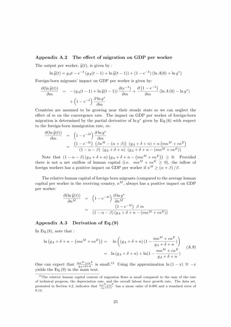
related to the net migration rate because of the capital dilution effect associated withlabour force growth, n. However, this effect is counterbalanced by the positive impactof the human capital content of migration flows (mκM + eκE). The net effect of mi-gration is therefore ambiguous and depends on the relative human capital contributionof foreign- and native-born migrants (κM and κE), net migration rates (m and e) andparameters of the production function (α and β).In this framework, ceteris paribus, the inflow of foreign workers will have a positiveimpact on long-term GDP per worker, and hence on productivity growth around thesteady state, only if new migrants are more qualified, on average, than the residentpopulation (κM > 1). However, this is not a sufficient condition, as the human capitalof migrants should also offset the capital dilution effect. Indeed, it may be shown that,provided there is not a net outflow of human capital associated with total net migration(i.e., mκM +eκE ≥ 0), κM ≥ (α+ β) /β is a sufficient condition for migration to have apositive impact on GDP per worker (see Appendix A.2). Below that threshold, however,the impact will depend on other parameters of the model.

The fact that migration has a positive impact on GDP per worker if and only ifits contribution to human capital accumulation more than compensates for the effecton capital dilution is a direct consequence of the augmented Solow-Swan theoreticalframework. This would not have necessarily been the case in an endogenous growthframework or in a framework that considers the imperfect substitution of natives andimmigrants in production (Manacorda et al., 2012; Ottaviano and Peri, 2012).

8

4 Econometric analysis

4.1 Empirical Model Specification

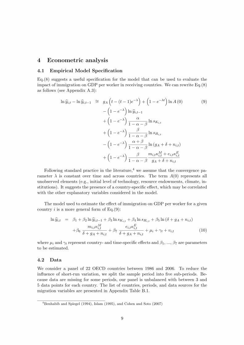
Eq.(8) suggests a useful specification for the model that can be used to evaluate theimpact of immigration on GDP per worker in receiving countries. We can rewrite Eq.(8)as follows (see Appendix A.3):

ln yi,t − ln yi,t−1∼= gA

(t− (t− 1)e−λ

)+(

1− e−λt)

lnA (0) (9)

−(

1− e−λ)

ln yi,t−1

+(

1− e−λ) α

1− α− βln sKi,t

+(

1− e−λ) β

1− α− βln sHi,t

−(

1− e−λ) α+ β

1− α− βln (gA + δ + ni,t)

+(

1− e−λ) β

1− α− βmi,tκ

Mi,t + ei,tκ

Ei,t

gA + δ + ni,t

Following standard practice in the literature,4 we assume that the convergence pa-rameter λ is constant over time and across countries. The term A(0) represents allunobserved elements (e.g., initial level of technology, resource endowments, climate, in-stitutions). It suggests the presence of a country-specific effect, which may be correlatedwith the other explanatory variables considered in the model.

The model used to estimate the effect of immigration on GDP per worker for a givencountry i is a more general form of Eq.(9):

ln yi,t = β1 + β2 ln yi,t−1 + β3 ln sKi,t + β4 ln sHi,t + β5 ln (δ + gA + ni,t)

+β6mi,tκ

Mi,t

δ + gA + ni,t+ β7

ei,tκEi,t

δ + gA + ni,t+ µi + γt + vi,t (10)

where µi and γt represent country- and time-specific effects and β1, ..., β7 are parametersto be estimated.

4.2 Data

We consider a panel of 22 OECD countries between 1986 and 2006. To reduce theinfluence of short-run variation, we split the sample period into five sub-periods. Be-cause data are missing for some periods, our panel is unbalanced with between 3 and5 data points for each country. The list of countries, periods, and data sources for themigration variables are presented in Appendix Table B.1.

4Benhabib and Spiegel (1994), Islam (1995), and Cohen and Soto (2007)

9

To assess the human capital content of migration flows, we compile a unique dataset of net migration flows that includes place of birth and educational attainment. Dataon international migration in OECD countries are relatively scarce. Most available dataare related to the characteristics of the stock of immigrants, whereas we require dataon the characteristics of immigrant flows to estimate Eq.(10). Indeed, the main sourcesof data on international migration are the population censuses, which provide compa-rable migration stock data for recent census years. For example, Artuc et al. (2013)provide information on gender, country of origin, and educational level of foreign-bornpopulations in 1990 and 2000. These data were extended by Brucker et al. (2013) for20 OECD countries for two additional census years, 1980 and 2010. Moreover, theyimpute missing information to compile data on the foreign-born population from 1980to 2010 at 5-year intervals. Furthermore, the OECD (2008) database on immigrants(DIOC) includes additional information on labour market outcomes and the durationof stay for immigrants living in OECD countries using the 2000 round of populationcensuses. Note that these data do not indicate where the tertiary diploma was obtainednor do they account for differences in skills, including language proficiency.Additional sources of information on immigrants include the OECD International Mi-gration Database and the UN International Migration Flows Database. However, thesedata are not harmonized and are not comparable across countries. Moreover, out-flows are generally unregulated and pose more measurement problems than inflows.Therefore, it is not possible to reconstruct comparable measures of net migration flows.Furthermore, data on immigrant flows concern only non-nationals (foreigners) while mi-gration also involves nationals (citizens). Note that, unlike country of birth, citizenshipchanges over time with naturalization, which may compromise the comparison acrosscountries at different time periods. Finally, statistics available on migration flows usu-ally do not distinguish education levels.

Consequently, an important part of the background work for this study has been togather and produce comparable data on net migration by country of birth and educa-tional attainment.Data on net migration flows by place of birth are directly available from the borderstatistics for Australia, New Zealand, and the United Kingdom and from populationregisters for Germany, the Netherlands, and Switzerland. For the 16 other countries,net migration flows of the native-born (E) are computed as a residual using a basicdemographic equation (Appendix B)5. Data on the native-born population are mainlycollected from population censuses. We impute missing information on the native-bornpopulation between census years following the United Nations (2009) methodology.Data on births, deaths and total net migration flows come from the OECD Populationand Vital Statistics data set. Note that net migration data (for both nationals andnon-nationals) has fewer comparability problems than the available data on inflows andoutflows of foreign citizens cited above. Finally, foreign-born net migration (M) is cal-culated as the difference between total net migration obtained from the OECD database

5For the countries for which data on native-born net migration are directly available, there is a strongcorrelation between data computed from population censuses and published data on native-born netmigration.

10

and native-born net migration computed from the native population.

Although data on the educational attainment of the immigrant population in OECDcountries are accessible, for example from Brucker et al. (2013), to the best of ourknowledge no data on the education level of immigrant flows are available. Becausethe education or skill level of immigrants, regardless of their date of arrival, does notaccount for the changes in their education and skill level over time, we compile data onthe educational attainment of recent immigrants. More precisely, we use the share of re-cent foreign-born migrants (i.e., those who have been in the host country for fewer than5 years) who have completed their tertiary education6 as a measure of the (average)human capital that each foreign-born immigrant brings to the host country (hM ). Thisshare is then compared to the corresponding figure for the total resident population atthe beginning of the period to compute κM . The data come from labour force surveydata for European countries and the United States and from population censuses forother OECD countries. Note that these data provide information only on immigrantswho still reside in the host country at the end of the observation period. No data areavailable on the skill composition of immigrants who left the host country during theperiod.

To calculate κE , we take advantage of the DIOC, which provides data for peopleborn in the OECD and living in another country circa 2000 including educational attain-ment, age, and duration of stay. The educational structure of native-born expatriatesis directly observed from this data source for those who emigrated between 1990–1994and 1998–2002. The former is approximated by OECD expatriates with 5 to 10 yearsof residence abroad in 2000 and the latter by OECD expatriates with fewer than 5years of residence abroad in 2000. Data are then linearly extrapolated for other periods(1986–1990, 1994–1998, and 2002–2006). Note that data on the education structure ofthe resident population come from Lutz et al. (2007).

The data clearly show that net migration of the native-born tends to be negativein most OECD countries over the period considered while the reverse is true for theforeign-born (Appendix Table B.2). Furthermore, net migration of the native-bornis non-negligible, and OECD expatriates are, on average, significantly more qualifiedthan both foreign-born migrants (Appendix Table B.3) and the resident population.The capacity to distinguish between net migration of the foreign-born and that of thenative-born is therefore essential to estimating the full impact of migration on host coun-tries. Note that recent immigrants to OECD countries are, on average, better educatedthan the resident population (Appendix Table B.4), which is in line with the findingsof Manacorda et al. (2012) and Dustmann et al. (2012) on migrant stocks. The notableexception is the United States where recent immigrants are slightly less educated, onaverage, than the resident population.

Data on GDP and the working age population (foreign- and native-born) come from

6People who have completed 5 to 6 ISCED education levels.

11

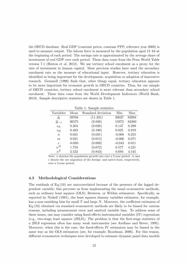
the OECD database. Real GDP (constant prices, constant PPP, reference year 2000) isused to measure output. The labour force is measured by the population aged 15–64 atthe beginning of each period. The savings rate is approximated by the average share ofinvestment of real GDP over each period. These data come from the Penn World Tableversion 7.1 (Heston et al , 2012). We use tertiary school enrolment as a proxy for therate of investment in human capital. Most previous studies have used the secondaryenrolment rate as the measure of educational input. However, tertiary education isidentified as being important for the development, acquisition or adoption of innovativeresearch. Gemmell (1996) finds that, other things equal, tertiary education appearsto be more important for economic growth in OECD countries. Thus, for our sampleof OECD countries, tertiary school enrolment is more relevant than secondary schoolenrolment. These data come from the World Development Indicators (World Bank,2013). Sample descriptive statistics are shown in Table 1.

Table 1: Sample statistics

Variables Mean Standard deviation Min Max

yt 39768 (11.331) 20027 92994yt−1 36575 (9.826) 15972 83280sK 0.204 (0.028) 0.147 0.289sH 0.483 (0.190) 0.025 0.919n 0.031 (0.031) -0.008 0.255m 0.021 (0.015) -0.006 0.071e -0.005 (0.009) -0.043 0.011κM 1.758 (0.672) 0.577 4.221κE 2.522 (0.843) 0.694 4.545

Note: n denotes the population growth rate over a 5-year period. m ande denote the net migration of the foreign- and native-born, respectively,over a 5-year period.

4.3 Methodological Considerations

The residuals of Eq.(10) are autocorrelated because of the presence of the lagged de-pendent variable; this prevents us from implementing the usual econometric methods,such as ordinary least squares (OLS), Between, or Within estimators. Specifically, asreported by Nickell (1981), the least squares dummy variables estimator, for example,has a non-vanishing bias for small T and large N . Moreover, the coefficient estimates ofEq.(10) obtained via standard econometric methods are likely to be biased for variousreasons, including measurement error and omitted variable bias. To address some ofthese issues, one may consider using fixed-effects instrumental variables (IV) regressions(e.g., two-stage least squares (2SLS)). The problem is that the first-stage statistics ofa 2SLS regression often has many weak instruments (see Arellano and Bover, 1995).Moreover, when this is the case, the fixed-effects IV estimators may be biased in thesame way as the OLS estimators (see, for example, Roodman, 2006). For this reason,different econometric techniques were developed to estimate dynamic panel data models

12

with short time dimensions in which lagged values of the explanatory endogenous vari-ables are used as instruments. These methods control for endogeneity and measurementerror for the lag of yt and other explanatory variables.

In our study, we use SYS-GMM, as proposed by Arellano and Bover (1995), whichcombines a regression in differences with one in levels. Blundell and Bond (1998) reportMonte Carlo evidence that the inclusion of a level regression in the estimation leadsto a reduction of the potential bias in small samples and asymptotic inaccuracy in thedifference estimator.7 The consistency of the GMM estimator relies on the validity ofthe instruments introduced in the model and the assumption that the error terms areuncorrelated8. To obtain valid instruments, we followed some of the recommendationsprovided by Roodman (2009) and Bazzi and Clement (2013); the former address theproblem of too many instruments,9 and the latter address the fact that common instru-mental variable approaches can lead to opaquely weak or opaquely invalid instruments.One of them is to limit the lag depth; the other is ‘collapsing’ the instrument set (seeRoodman, 2009). The former implies a selection of lags to be included in the instru-ment set, making the instrument count linear in T . The latter embodies a differentbelief about the orthogonality condition: it no longer needs to be valid for any one timeperiod but still for each lag, again making the instrument count linear in T . A combina-tion of both techniques makes the instrument count invariant to T . In our case, we usecollapsed two-period lags from all variables included in the estimation as the (internal)instrument sets.10 Moreover, following Bazzi and Clement (2013), internal instrumentsmay not be sufficient in dynamic models estimated by SYS-GMM techniques; thus, wealso include an external instrument11 that has already been used in other publishedwork (Altonji and Card, 1991; Card, 2001; Dustmann et al., 2005). This procedure is

7The first-differenced GMM estimator is based on writing the equation at hand as a dynamic paneldata model, taking first-differences to remove the unobserved time-invariant country-specific effectsand then instrumenting the right-hand-side variables in the first-differenced equations using levels ofthe series lagged two periods or more. This is performed under the assumption that the time-varyingdisturbances in the original level equations are not serially correlated.

8Note that we are aware that there exist doubts in the literature about the consistency of the SYS-GMM estimator when used with macroeconomic data. For instance, compared to the first-differencedGMM estimator, when implementing the SYS-GMM estimator, an additional assumption must be madeto ensure the validity of the additional instrumental variables used in the level equation; indeed, thecountry fixed effects are assumed to be uncorrelated with lagged differences in the dependent variable,an assumption that is actually quite complicated to assess in an empirical study. We acknowledgethese drawbacks as limitations of the paper; however, as accurately noted by a referee, the SYS-GMMestimator is the best available estimator in this context (compared to other estimation methods).

9The main small-sample problem associated with numerous instruments is that a large instrumentcollection overfits endogenous variables even as it weakens the Hansen test of the instruments’ jointvalidity. Specifically, as Roodman (2009) states, “if for instance T = 3, the SYS-GMM generates onlytwo instruments per instrumenting variable. However, as T rises, the instrument count can easily growlargely relative to the sample size, making some asymptotic results about the estimators and relatedspecification tests misleading.” See the paper for a more complete discussion of this issue.

10Note that similar results are obtained with the collapsed three-period lags from all variables includedin the estimation as the instruments sets.

11We also use the collapsed two-period lags from past immigrant concentrations as external instrumentsets. Similar results are obtained with the collapsed three-period lags.

13

typically implemented by using the share of immigrants in the population at the begin-ning of the period as an instrumental variable for immigrant inflows during the period.Indeed, immigrants tend to settle where networks exist (Bartel, 1989; Jaeger, 2007), andpast immigration concentrations are unlikely to be related to current economic shocks.Here, the stock of high-skilled immigrants already residing in a country from Brucker etal. (2013) is used as an instrument for the inflows of highly skilled immigrants. Indeed,an OECD country with a larger high-skilled immigrant population attracts larger flowsof highly skilled immigrants.

Finally, we consider three specification tests to address the consistency of the SYS-GMM estimator. The first is a serial correlation test, which tests the null hypothesisof no first-order serial correlation and no second-order serial correlation in the residualsof the first-differenced equation. The second is a Sargan test of overidentifying restric-tions, which examines the overall validity of the instruments by comparing the momentconditions to their sample analogue. A finite sample correction is made to the two-stepcovariance matrix using Windmeijer’s (2005) method. The third is a difference Sargantest, denoted as Diff-Sargan, proposed by Blundell and Bond (1998), which examinesthe null hypothesis of mean stationarity for the SYS-GMM estimator. These statistics,called incremental Sargan test statistics, are the difference between the Sargan statisticsfor first-differenced GMM and SYS-GMM. It is asymptotically χ2 distributed with kdegrees of freedom, where k is the number of additional moment conditions.

4.4 Econometric Results

Before turning to the regression equations, we first consider the pooling restrictionsimplicit in Eq.(10) and test whether key parameters are equal across countries (i.e.,βij = βi,∀i = [1, 7], j = [1, 22]), which would imply that pooling time series and cross-sectional data are valid in our growth regression context. Specifically, we employ amulti-step procedure to test pooling restrictions in our system of 22 OECD members;hypotheses of interest are tested by means of a likelihood-ratio statistic. This pro-cedure is in the spirit of the approach of Hsiao (1986). Our results (available uponrequest) provide evidence that common coefficients can be assumed across countries,and consequently, pooling time series and cross sectional data appears to be reason-able in this context. However, the additional restriction that µj = µ,∀j = [1, 22] wasstrongly rejected by the data, implying that Eq.(10) includes individual country effects.Furthermore, the fixed effect specification is more appropriate in our growth equationframework.

We then estimate Eq.(10) using data for 22 OECD countries from 1986–2006. Theresults for the SYS-GMM estimation are reported in Table 212. Two types of specifica-tions are considered. The first is the standard augmented Solow model, which serves asa benchmark. The results for this specification are presented in column 1. The secondincludes the human capital content of the net migration variables as specified in Eq.(10).

12The estimation results using pooled OLS and FE estimators are presented in Appendix Table C.1

14

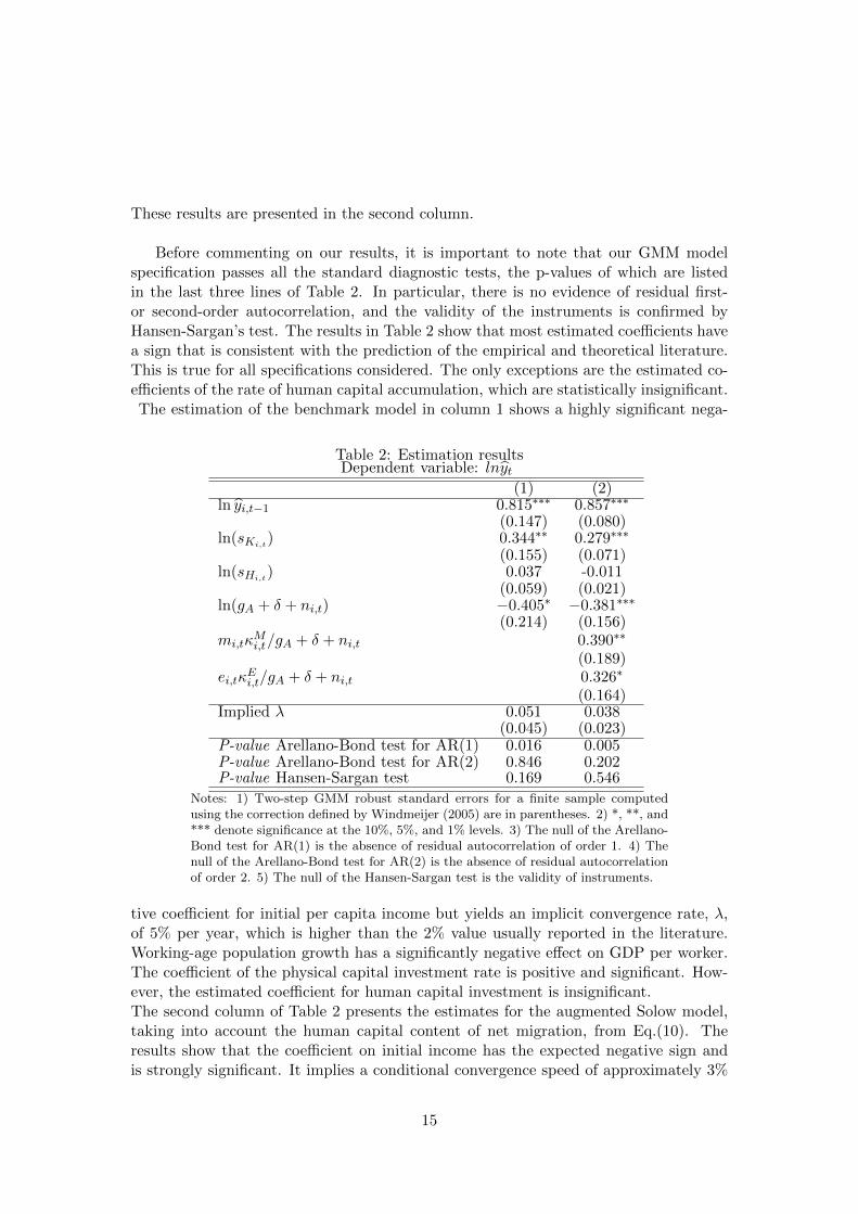
These results are presented in the second column.

Before commenting on our results, it is important to note that our GMM modelspecification passes all the standard diagnostic tests, the p-values of which are listedin the last three lines of Table 2. In particular, there is no evidence of residual first-or second-order autocorrelation, and the validity of the instruments is confirmed byHansen-Sargan’s test. The results in Table 2 show that most estimated coefficients havea sign that is consistent with the prediction of the empirical and theoretical literature.This is true for all specifications considered. The only exceptions are the estimated co-efficients of the rate of human capital accumulation, which are statistically insignificant.The estimation of the benchmark model in column 1 shows a highly significant nega-

Table 2: Estimation resultsDependent variable: lnyt

(1) (2)ln yi,t−1 0.815∗∗∗ 0.857∗∗∗

(0.147) (0.080)ln(sKi,t

) 0.344∗∗ 0.279∗∗∗

(0.155) (0.071)ln(sHi,t

) 0.037 -0.011(0.059) (0.021)

ln(gA + δ + ni,t) −0.405∗ −0.381∗∗∗

(0.214) (0.156)mi,tκ

Mi,t/gA + δ + ni,t 0.390∗∗

(0.189)ei,tκ

Ei,t/gA + δ + ni,t 0.326∗

(0.164)Implied λ 0.051 0.038

(0.045) (0.023)P-value Arellano-Bond test for AR(1) 0.016 0.005P-value Arellano-Bond test for AR(2) 0.846 0.202P-value Hansen-Sargan test 0.169 0.546

Notes: 1) Two-step GMM robust standard errors for a finite sample computedusing the correction defined by Windmeijer (2005) are in parentheses. 2) *, **, and*** denote significance at the 10%, 5%, and 1% levels. 3) The null of the Arellano-Bond test for AR(1) is the absence of residual autocorrelation of order 1. 4) Thenull of the Arellano-Bond test for AR(2) is the absence of residual autocorrelationof order 2. 5) The null of the Hansen-Sargan test is the validity of instruments.

tive coefficient for initial per capita income but yields an implicit convergence rate, λ,of 5% per year, which is higher than the 2% value usually reported in the literature.Working-age population growth has a significantly negative effect on GDP per worker.The coefficient of the physical capital investment rate is positive and significant. How-ever, the estimated coefficient for human capital investment is insignificant.The second column of Table 2 presents the estimates for the augmented Solow model,taking into account the human capital content of net migration, from Eq.(10). Theresults show that the coefficient on initial income has the expected negative sign andis strongly significant. It implies a conditional convergence speed of approximately 3%

15

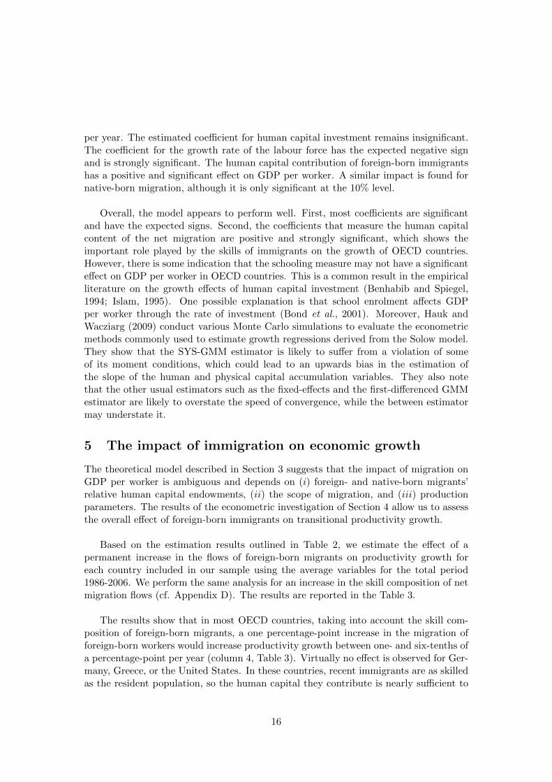
per year. The estimated coefficient for human capital investment remains insignificant.The coefficient for the growth rate of the labour force has the expected negative signand is strongly significant. The human capital contribution of foreign-born immigrantshas a positive and significant effect on GDP per worker. A similar impact is found fornative-born migration, although it is only significant at the 10% level.

Overall, the model appears to perform well. First, most coefficients are significantand have the expected signs. Second, the coefficients that measure the human capitalcontent of the net migration are positive and strongly significant, which shows theimportant role played by the skills of immigrants on the growth of OECD countries.However, there is some indication that the schooling measure may not have a significanteffect on GDP per worker in OECD countries. This is a common result in the empiricalliterature on the growth effects of human capital investment (Benhabib and Spiegel,1994; Islam, 1995). One possible explanation is that school enrolment affects GDPper worker through the rate of investment (Bond et al., 2001). Moreover, Hauk andWacziarg (2009) conduct various Monte Carlo simulations to evaluate the econometricmethods commonly used to estimate growth regressions derived from the Solow model.They show that the SYS-GMM estimator is likely to suffer from a violation of someof its moment conditions, which could lead to an upwards bias in the estimation ofthe slope of the human and physical capital accumulation variables. They also notethat the other usual estimators such as the fixed-effects and the first-differenced GMMestimator are likely to overstate the speed of convergence, while the between estimatormay understate it.

5 The impact of immigration on economic growth

The theoretical model described in Section 3 suggests that the impact of migration onGDP per worker is ambiguous and depends on (i) foreign- and native-born migrants’relative human capital endowments, (ii) the scope of migration, and (iii) productionparameters. The results of the econometric investigation of Section 4 allow us to assessthe overall effect of foreign-born immigrants on transitional productivity growth.

Based on the estimation results outlined in Table 2, we estimate the effect of apermanent increase in the flows of foreign-born migrants on productivity growth foreach country included in our sample using the average variables for the total period1986-2006. We perform the same analysis for an increase in the skill composition of netmigration flows (cf. Appendix D). The results are reported in the Table 3.

The results show that in most OECD countries, taking into account the skill com-position of foreign-born migrants, a one percentage-point increase in the migration offoreign-born workers would increase productivity growth between one- and six-tenths ofa percentage-point per year (column 4, Table 3). Virtually no effect is observed for Ger-many, Greece, or the United States. In these countries, recent immigrants are as skilledas the resident population, so the human capital they contribute is nearly sufficient to

16

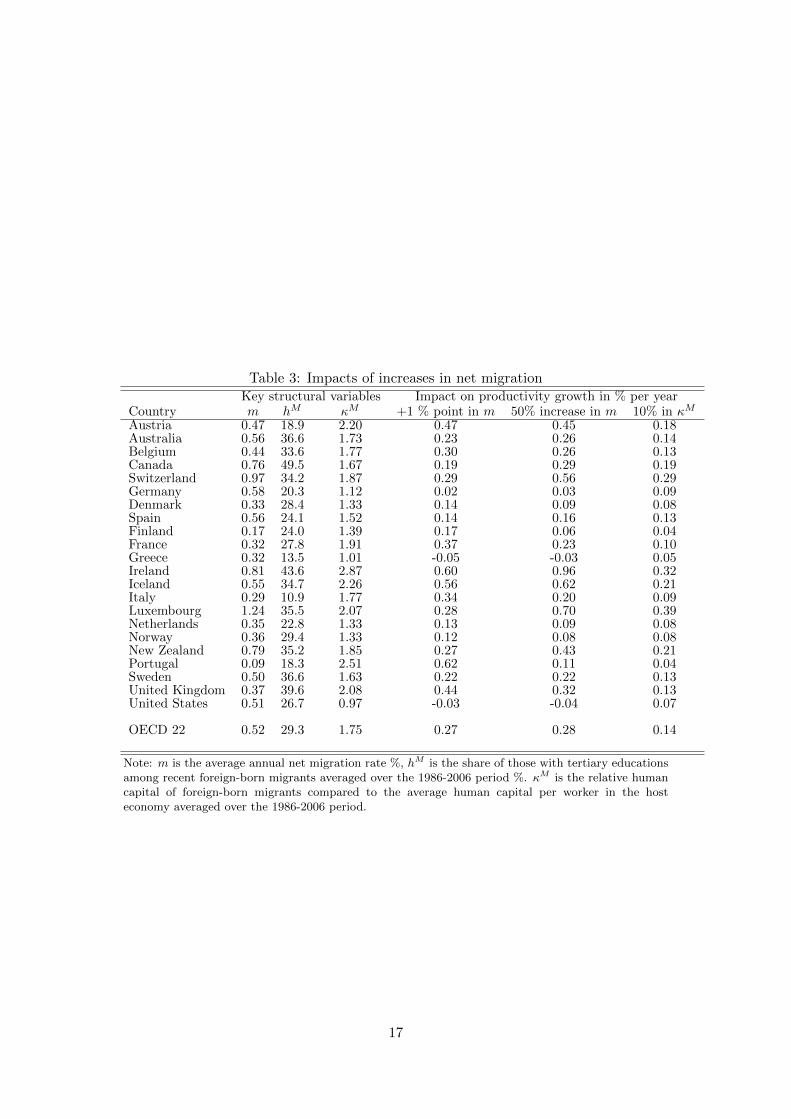
Table 3: Impacts of increases in net migrationKey structural variables Impact on productivity growth in % per year

Country m hM κM +1 % point in m 50% increase in m 10% in κM

Austria 0.47 18.9 2.20 0.47 0.45 0.18Australia 0.56 36.6 1.73 0.23 0.26 0.14Belgium 0.44 33.6 1.77 0.30 0.26 0.13Canada 0.76 49.5 1.67 0.19 0.29 0.19Switzerland 0.97 34.2 1.87 0.29 0.56 0.29Germany 0.58 20.3 1.12 0.02 0.03 0.09Denmark 0.33 28.4 1.33 0.14 0.09 0.08Spain 0.56 24.1 1.52 0.14 0.16 0.13Finland 0.17 24.0 1.39 0.17 0.06 0.04France 0.32 27.8 1.91 0.37 0.23 0.10Greece 0.32 13.5 1.01 -0.05 -0.03 0.05Ireland 0.81 43.6 2.87 0.60 0.96 0.32Iceland 0.55 34.7 2.26 0.56 0.62 0.21Italy 0.29 10.9 1.77 0.34 0.20 0.09Luxembourg 1.24 35.5 2.07 0.28 0.70 0.39Netherlands 0.35 22.8 1.33 0.13 0.09 0.08Norway 0.36 29.4 1.33 0.12 0.08 0.08New Zealand 0.79 35.2 1.85 0.27 0.43 0.21Portugal 0.09 18.3 2.51 0.62 0.11 0.04Sweden 0.50 36.6 1.63 0.22 0.22 0.13United Kingdom 0.37 39.6 2.08 0.44 0.32 0.13United States 0.51 26.7 0.97 -0.03 -0.04 0.07

OECD 22 0.52 29.3 1.75 0.27 0.28 0.14

Note: m is the average annual net migration rate %, hM is the share of those with tertiary educationsamong recent foreign-born migrants averaged over the 1986-2006 period %. κM is the relative humancapital of foreign-born migrants compared to the average human capital per worker in the hosteconomy averaged over the 1986-2006 period.

17

offset the capital dilution effect. Note that the very small negative effect of foreign-bornmigration on productivity growth in Greece and the United States represents only one-tenth of the negative impact of a comparable increase in the natural population growthrate, n.A one percentage-point increase in net migration is not necessarily comparable acrosscountries, as it represents quite distinct migration shocks. If we consider a 50% increasein the net migration rate of the foreign-born, all else being equal, we find that in allbut two countries, the change in productivity growth is positive (column 5, Table 3).Still, the migration growth effect is small for all countries except Ireland, Iceland, andLuxembourg, where the increase in productivity growth is more than six-tenths of apercentage-point per year.

To compare our results with regard to recent empirical literature, we should look atthe effect on the demographic ratio of working age to total population (Appendix E)–in addition to the effect on GDP per worker (referring to the working age population)outlined in Table 3. Foreign-born migration flows improved this ratio in all OECD coun-tries. In Greece and the United States, the positive demographic effect compensatesfor the small negative effect on productivity growth. Thus, foreign-born, permanentmigration flows increase GDP per capita in all of the OECD countries considered (Ap-pendix Table E1). These results are in line with the findings of recent empirical studiesbased on migration stock data, although the positive effect of foreign-born migrationwe observe seems smaller in magnitude. For instance, the results of Felbermayr et al.(2010) indicate that a 10% increase in the migration stock leads to a per capita in-come gain of 2.2%. Ortega and Peri (2014) also find ”‘a qualitatively large effect: a 10percentage-point difference in the share of foreign born in the population”’ seems to be”‘associated with differences in income per person by a factor close to 2”’.

Moreover, in this framework, adopting more selective migration policies has a sys-tematically positive impact on productivity growth. Column 6 shows that a 10% in-crease in the relative share of immigrants with tertiary educations compared to the res-ident population increases the productivity growth rate between one- and four-tenthsof a percentage-point. It is also worth noting that increasing the education level of newimmigrants will have a positive impact on productivity growth in countries such as Ger-many, Greece, and the United States, where foreign-born immigrants are as educated asthe resident population. For the remaining countries, immigrants are highly educatedcompared to the resident population, and given the skill level of recent immigrants,increasing net migration seems to have a more sizable impact on productivity growththan more selective policies.

6 Conclusion

By estimating a structural model, this paper has sought to re-examine the effects ofpermanent migration flows by country of origin and skill level on economic growth. Ourempirical results support the theoretical model and demonstrate a positive impact from

18

migrants’ human capital on GDP per worker. Besides, the contribution of immigrants tohuman capital accumulation tends to dominate the capital dilution effect. However, thenet effect is fairly small, even in countries that have highly selective migration policies.Indeed, a 50% increase in net migration of the foreign-born generates, on average, anincrease of three-tenths of a percentage-point in productivity growth per year in OECDcountries. Increasing the selectivity of migration policies does not appear to have amore marked effect on productivity growth, except perhaps in countries where recentimmigrants are somewhat less educated than the resident population.

Obviously, one could argue that our model only partially captures the effects of mi-gration on economic growth. For example, migration changes the domestic age structureof host countries because migrants tend to be concentrated in more active age groupscompared to natives, and thereby reducing dependency ratios. There is also some ev-idence that immigrants tend to be complementary to natives, as they may allow somenative workers to devote time to more productive jobs. Further, immigrants may bringsome assets with them, thereby contributing to physical capital accumulation in thehost country. Moreover, skilled immigrants may contribute to research and boost inno-vation and technological progress. Further research is needed to account for these effectsbefore one can definitively state the full impact of migration on economic growth. Thatsaid, our results provide evidence that one should not expect large gains (or significantloses) in terms of productivity from migration.

19

References

Alesina, A., Harnoss, J., Rapoport, H. (2013) Birthplace Diversity and Economic Pros-perity,. Working Paper 18699. National Bureau of Economic Research.

Altonji, J. G., and Card, D. (1991) The Effects of Immigration on the Labor MarketOutcomes of Less skilled Natives, ch. 7 in J. M. Abowd and R. B. Freeman (eds),Immigration, Trade, and the Labor Market, Chicago, IL, University of Chicago Press,201-34.

Andersen, T. and Dalgaard, C. J.(2011) Flows of people, flows of ideas, and the inequal-ity of nations, Journal of Economic Growth, 16, 1-32.

Angrist J. D. and Kugler A. D. (2003) Protective or Counter-Productive? LabourMarket Institutions and the Effect of Immigration on EU Natives, Economic Journal,113, F302-31.

Arellano, M. and Bover.O. (1995) Another Look at the Instrumental Variable Estima-tion of Error-Components Models, Journal of Econometrics, 68, 29-52.

Artuc, E., Docquier, F.,Ozden, C. and Ch. Parsons (2013) A global assessment of humancapital mobility: the role of non-OECD destinations

Auerbach A. and P. Oreopoulos (1999) Analysing the Fiscal Impact of US Immigration,American Economic Review, 89, 176-80.

Barro, R. and X. Sala-i-Martin (1995) Economic Growth, McGraw-Hill, New York.

Bartel, A. P.(1989) Where Do the New US Immigrants Live?, Journal of Labor Eco-nomics, 7, 371-91.

Bazzi, S. and Clement M. A (2013) Blunt instruments: avoiding common pitfalls inidentifying the causes of economic growth, American Economic Journal: Macroeco-nomics, 5, 152-86.

Benhabib, J.and Spiegel, M.M. (1994) The role of human capital in economic develop-ment: Evidence from aggregate cross-country data, Journal of Monetary Economics,34, 143-73.

Blundell, R. and S. Bond. (1998) Initial Conditions and Moment Restrictions in Dy-namic Panel Data Models, Journal of Econometrics, 87, 115-43.

Bond, S., Hoeffler, A. and J. Temple. (2001) GMM Estimation of Empirical GrowthModels, CEPR discussion paper no. 3048 .

Borjas G.J. (2003) The Labor Demand Curve is Downward Sloping: Reexamining theImpact of Immigration on the Labor Market, Quarterly Journal of Economics, 118,1335-74.

Boubtane, E., Coulibaly, D. and Rault, C. (2013) Immigration, Growth, and Unem-ployment: Panel VAR Evidence from OECD Countries, Review of Labour Economicsand Industrial Relations, 27, 399-420.

Bretschger, L. (2001) Labor supply, Migration, and Long-term development, Openeconomies review, 12, 5-27.

Brucker H., Capuano, S. and Marfouk, A. (2013) Education, gender and internationalmigration: insights from a panel-dataset 1980-2010, mimeo.

20

Card, D. (2001) Immigrant Inflows, Native Outflows, and the Local Labor MarketImpacts of Higher Immigration, Journal of Labor Economics, 19, 22-64.

Cohen, D. and Soto,M. (2007) Growth and human capital: good data, good results,Journal of Economic Growth, 12, 51-76.

di Giovanni, J., Levchenko,A.A., and Ortega, F. (2014) A Global View of Cross-BorderMigration, Journal of the European Economic Association, 13(1), 168-202.

Dolado, J., A. Goria, and A. Ichino, (1994) Immigration, Human Capital and Growthin the Host Country: Evidence from Pooled Country Data, Journal of PopulationEconomics, 7, 193-215.

Dustmann, C., Fabbri, F., and Preston, I. (2005), The Impact of Immigration on theBritish Labour Market, The Economic Journal, 115(507), F324-41.

Dustmann, C., Frattini, T., and Lanzara, G. (2012) Educational achievement of second-generation immigrants: an international comparison, Economic Policy, 27, 143-85.

Dustmann, C.and Mestres, J. (2010) Remittances and Temporary Migration, Journalof Development Economics, 92(1), 62-70.

Gemmell, N. (1996) Evaluating the Impacts of Human Capital Stocks and Accumula-tion on Economic Growth: Some New Evidence, Oxford Bulletin of Economics andStatistics, 58, 9-28.

Felbermayr, G., S. Hiller, and Sala,D.(2010) Does Immigration Boost Per Capita In-come?, Economics Letters, 107, 177-79.

Hauk, W. and Wacziarg,R. (2009) A Monte Carlo study of growth regressions, Journalof Economic Growth, 14(2), 103-47.

Heston A., Summers R. and Aten B. (2012) Penn World Table Version 7.1, Centerfor International Comparisons of Production, Income and Prices at the University ofPennsylvania.

Hsiao, C.(1986) Analysis of Panel Data, Cambridge University Press, Cambridge, MA.

Hunt J. and M. Gauthier-Loiselle, (2010) How Much Does Immigration Boost Innova-tion?, American Economic Journal: Macroeconomics, 2(2), 31-56.

Islam, N. (1995) Growth Empirics: A Panel Data Approach, The Quarterly Journal ofEconomics, 110, 1127-70.

Jaeger, D. (2007) Green Cards and the Location Choices of Immigrants in the UnitedStates, 19712000, Research in Labor Economics, 27, 131-83.

Lubotsky D. (2007) Chutes or Ladders? A Longitudinal Analysis of Immigrant Earn-ings, Journal of Political Economy, 115(5), 820-67.

Lundborg, P. and Segerstrom, P. (2000) International Migration and Growth in Devel-oped Countries: A theoretical analysis, Economica, 67, 579-604.

Lundberg, P.and Segerstrom, P. (2002) The growth and welfare effects of internationalmass migration. Journal of International Economics, 56, 177-204

Lutz, W., Goujon, A., Samir, K. and Sanderson, W. (2007) Reconstruction of popula-tions by age, sex and level of educational attainment for 120 countries for 1970-2000,Vienna Yearbook of Population Research 2007, 193-235.

21

Manacorda, M., Manning, A. and Wadsworth, J. (2012) The Impact Of ImmigrationOn The Structure Of Wages: Theory And Evidence From Britain, Journal of theEuropean Economic Association, 10, 120-51.

Mankiw, G., D. Romer and D. Weil (1992) A Contribution to the Empirics of EconomicGrowth, Quarterly Journal of Economics, 107, 407-37.

Morley, B. (2006) Causality between economic growth and immigration: An ARDLbounds testing approach, Economics Letters, 90, 72-6.

Nickell, S. (1981) Biases in dynamic models with fixed effects, Econometrica, 49, 1417-26.

OECD(2008) A Profile of Immigrant Populations in the 21st Century: Data from OECDCountries, Paris.

OECD (2009) Recent Trends in International Migration, International Migration Out-look, Paris.

Ortega F. and Peri, G. (2009) The causes and Effects of International Migration: evi-dence from OECD countries 1980-2005, NBER Working Papers 14833.

Ortega F. and Peri G. (2014) Migration, Trade and Income, Journal of InternationalEconomics, 92, 231-51.

Ottaviano, G., I.,P. and Peri, G. (2012) Rethinking The Effect Of Immigration OnWages, Journal of the European Economic Association, 10, 152-97.

Robertson, P.E.(2002) Demographic shocks and human capital accumulation in theUzawa-Lucas model, Economics Letters, Elsevier, 74, pages 151-6.

Roodman, D. (2006) How to do xtabond2: An introduction to ‘Difference’ and ‘System’GMM in Stata, Center for Global development Working Paper 103.

Roodman, D. (2009) A note on the theme of too many instruments,Oxford Bulletin ofEconomics and Statistics, 71, 135-58.

Rowthorn, R. (2008) The Fiscal Impact of Immigration on the AdvancedEconomies.Oxford Review of Economic Policy, 24, 560-80.

Storesletten, K. (2000) Sustaining Fiscal Policy through Immigration, Journal of Polit-ical Economy, 108, 300-23.

United Nations (2009) Trends in International Migrant Stock: The 2008 Revision.

Walz, U. (1995) Growth (Rate) Effects of Migration, Zeitschrift fur Wirtschafts- undSozialwissenschaften, 115, 199-221.

Windmeijer, F. (2005) A finite sample correction for the variance of linear efficienttwo-step GMM estimators, Journal of Econometrics, 126, 25-51.

World Bank (2013) World Development Indicators, Washington, DC.

22

Appendix A The theoretical model

Appendix A.1 The speed of convergence

From the intensive form production function given by Eq.(4) in the main text, the rateof growth of income per effective worker is given by:

·y

y= α

·k

k+ β

·h

h(A.1)

We substitute Eq.(5) into Eq.(A.1) to get:

·y

y= α

(sK

y

k− (δ + gA + n)

)+β(sH

y

h−(δ + gA + n−

(m κM + e κE

)))(A.2)

The economy converges to a steady state defined by :

k∗ =

(sK

δ + gA + n

) 1−β1−α−β

(sH

δ + gA + n− (mκM + eκE)

) β1−α−β

h∗ =

(sK

δ + gA + n

) α1−α−β

(sH

δ + gA + n− (mκM + eκE)

) 1−α1−α−β

(A.3)

Note that at the steady state, using Eq.(A.3) we have:

sKy∗k∗

= (δ + gA + n)

sHy∗h∗

= δ + gA + n−(m κM + eκE

) (A.4)

Substituting Eq.(A.4) into Eq.(A.2) results in:

·y

y= α

(sK

y

k− sK

y∗k∗

)+ β

(sH

y

h− sH

y∗h∗

)Therefore:

·y

y= αsK

y∗k∗

((k

k∗

)α−1( h

h∗

)β− 1

)

+βsHy∗h∗

((k

k∗

)α( h

h∗

)β−1

− 1

)

(A.5)

23

Note that:(k

k∗

)α−1( h

h∗

)β− 1 = exp

((α− 1) ln

(k

k∗

)+ β ln

(h

h∗

))− 1.

Around the steady state (α− 1) ln(kk∗)+β ln

(hh∗)

is small, so we can use the exponentialapproximation ex = 1 + x to obtain:(

k

k∗

)α−1( h

h∗

)β− 1 = (α− 1) ln

(k

k∗

)+ β ln

(h

h∗

)(k

k∗

)α( h

h∗

)β−1

− 1 = α ln

(k

k∗

)+ (β − 1) ln

(h

h∗

) (A.6)

Substituting Eq.(A.4) and Eq.(A.6) into Eq.(A.5), we have:

·y

y= α (δ + gA + n)

((α− 1) ln

(k

k∗

)+ β ln

(h

h∗

))+β(δ + gA + n−

(m κM − e κE

))(α ln

(k

k∗

)+ (β − 1) ln

(h

h∗

))

Then:

·y

y= − (δ + gA + n)

[(1− α− β)ln

(y

y∗

)+ β

m κM + e κE

δ + gA + n

(ln

(y

y∗

)− ln

(h

h∗

))]For small m κM+e κE

δ+gA+n, βm κM+e κE

δ+gA+n

(ln(yy∗

)− ln

(hh∗))

can be neglected. So, the growth

rate as the economy converges to the steady state is:

·y

y= − (δ + gA + n) (1− α− β) ln

y

y∗= − (δ + gA + n) (1− α− β) (ln y − ln y∗)= −λ (ln y − ln y∗) ,

(A.7)

and thus the rate of convergence is given by:

λ = (1− α− β) (δ + gA + n)

The rate of growth as the economy converges to the steady state can be approximatedby:

·y

y=∂ ln y

∂t' −λ (ln y (t)− ln y∗)

This yields to :ln y (t)− ln y∗ ∼= e−λt (ln y (0)− ln y∗) (A.8)

where y(0) is income per effective worker at some initial date. Note that, assuming aconstant rate of convergence λ over time, Eq.(A.8) also holds between dates t and t−1.We obtain Eq.(7) in the main text.

24

Appendix A.2 The effect of migration on GDP per worker

The output per worker, y(t), is given by :

ln y(t) = gAt− e−λ (gA(t− 1) + ln y(t− 1)) + (1− e−λ) (lnA(0) + ln y∗)

Foreign-born migrants’ impact on GDP per worker is given by:

∂(ln y(t))

∂m= − (gA(t− 1) + ln y(t− 1))

∂(e−λ)

∂m+∂(1− e−λ

)∂m

(lnA (0)− ln y∗)

+(

1− e−λ) ∂ ln y∗

∂m

Countries are assumed to be growing near their steady state so we can neglect theeffect of m on the convergence rate. The impact on GDP per worker of foreign-bornmigration is determined by the partial derivative of ln y∗ given by Eq.(6) with respectto the foreign-born immigration rate, m:

∂(ln y(t))

∂m=

(1− e−λt

) ∂ ln y∗

∂m

=

(1− e−λt

) (βκM − (α+ β)

)(gA + δ + n) + α

(mκM + eκE

)(1− α− β) (gA + δ + n) (gA + δ + n− (mκM + eκE))

Note that (1− α− β) (gA + δ + n)(gA + δ + n−

(mκM + eκE

))≥ 0. Provided

there is not a net outflow of human capital (i.e. mκM + eκE ≥ 0), the inflow offoreign workers has a positive impact on GDP per worker if κM ≥ (α+ β) /β.

The relative human capital of foreign born migrants (compared to the average humancapital per worker in the receiving country, κM , always has a positive impact on GDPper worker:

∂(ln y(t))

∂κM=

(1− e−λt

) ∂ ln y∗

∂κM

=

(1− e−λt

)β m

(1− α− β) (gA + δ + n− (mκM + eκE))

Appendix A.3 Derivation of Eq.(9)

In Eq.(8), note that :

ln(gA + δ + n−

(mκM + eκE

))= ln

((gA + δ + n) (1− mκM + eκE

gA + δ + n)

)= ln (gA + δ + n) + ln(1− mκM + eκE

gA + δ + n)

(A.9)

One can expect that mκM+eκE

gA+δ+nis small.13 Using the approximation ln (1− x) ∼= −x

yields the Eq.(9) in the main text.

13The relative human capital content of migration flows is small compared to the sum of the rateof technical progress, the depreciation rate, and the overall labour force growth rate. The data set,

presented in Section 4.2, indicates that mκM+eκE

gA+δ+nhas a mean value of 0.095 and a standard error of

0.14.

25

Appendix B Data

This section presents the methodology used to estimate net migration by country ofbirth (see Appendix Table B.1 for data sources).

According to the basic demographic equation, the native-born population (NBP )14

at any point in time is equal to the native population at the previous point in time plusthe net migration of the native-born (NBM) and the natural increase in the population(number of births, B, in the country minus deaths of the native-born, NBD):

NBPt+1 = NBPt +Bt−t+1 −NBDt−t+1 +NBMt−t+1

Note that all births are by definition native, but deaths also include the foreign-born.In order to calculate the deaths of the native-born, we use the share of native-born inthe total population, corrected their age structure and mortality rates by age. Data ondeaths, births, and net migration are from the OECD database. Deaths by age groupcome from the World Health Organisation Mortality Database.

Native-born net migration is then given by:

NBMt−t+1 = NBPt+1 −NBPt − (Bt−t+1 −NBDt−t+1)

Foreign-born net migration is given by the difference between total net migration andthe net migration of the native-born as estimated above. When census data are used,the statistical adjustment was added to net migration of the foreign-born, except forFrance between 1990 and 1999 (to the native-born) and Italy (not included). Note thatthe majority of immigrants are of working age. We assume that 80% of the estimatednet migration as working age immigrants for the foreign- and native-born.

14In order to evaluate the stock of the native-born between census dates, we use an interpolationtechnique. This methodology is used by the United Nation Population Division to estimate the migrantstock in the Global Migration Database United Nations (2009).

26

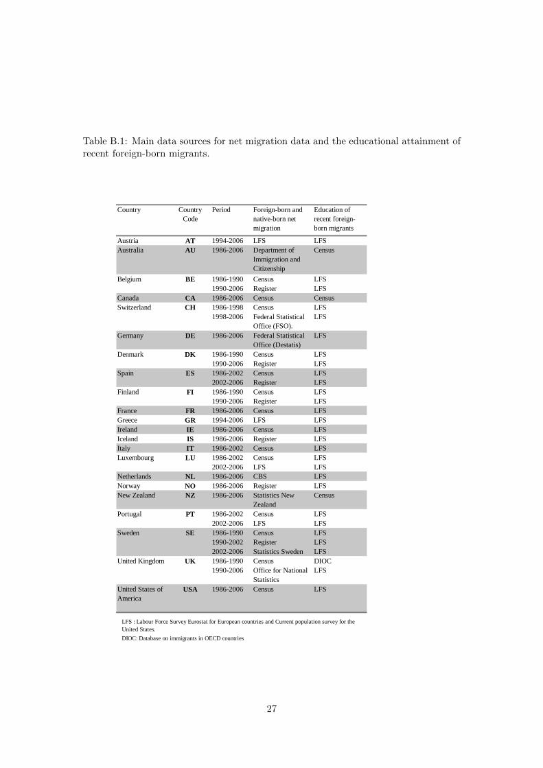
Table B.1: Main data sources for net migration data and the educational attainment ofrecent foreign-born migrants.

Austria AT 1994-2006 LFS LFSAustralia AU 1986-2006 Department of

Immigration and Citizenship

Census

Belgium 1986-1990 Census LFS1990-2006 Register LFS

Canada CA 1986-2006 Census CensusSwitzerland 1986-1998 Census LFS

1998-2006 Federal Statistical Office (FSO).

LFS

Germany DE 1986-2006 Federal Statistical Office (Destatis)

LFS

Denmark 1986-1990 Census LFS1990-2006 Register LFS

Spain 1986-2002 Census LFS2002-2006 Register LFS

Finland 1986-1990 Census LFS1990-2006 Register LFS

France FR 1986-2006 Census LFSGreece GR 1994-2006 LFS LFSIreland IE 1986-2006 Census LFSIceland IS 1986-2006 Register LFSItaly IT 1986-2002 Census LFSLuxembourg 1986-2002 Census LFS

2002-2006 LFS LFSNetherlands NL 1986-2006 CBS LFSNorway NO 1986-2006 Register LFSNew Zealand NZ 1986-2006 Statistics New

Zealand Census

Portugal 1986-2002 Census LFS2002-2006 LFS LFS

Sweden 1986-1990 Census LFS1990-2002 Register LFS2002-2006 Statistics Sweden LFS

United Kingdom 1986-1990 Census DIOC1990-2006 Office for National

StatisticsLFS

DIOC: Database on immigrants in OECD countries

SE

BE

LFS : Labour Force Survey Eurostat for European countries and Current population survey for the United States.

CH

DK

ES

FI

LU

PT

UK

United States of America

USA 1986-2006 Census LFS

Country Period Foreign-born and native-born net migration

Education of recent foreign-born migrants

Country Code

27

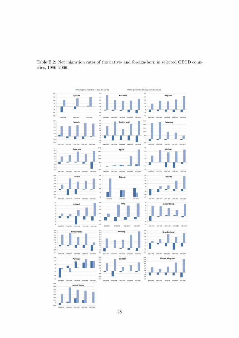
Table B.2: Net migration rates of the native- and foreign-born in selected OECD coun-tries, 1986–2006.

-150

-100

-50

0

50

100

150

200

1994-1998 1998-2002 2002-2006

Austria

-200

-100

0

100

200

300

400

500

1986-1990 1990-1994 1994-1998 1998-2002 2002-2006

Australia

-100

-50

0

50

100

150

200

250

1986-1990 1990-1994 1994-1998 1998-2002 2002-2006

Belgium

-400

-200

0

200

400

600

800

1000

1986-1990 1990-1994 1994-1998 1998-2002 2002-2006

Canada

-150

-100

-50

0

50

100

150

200

250

300

1986-1990 1990-1994 1994-1998 1998-2002 2002-2006

Switzerland

-500

0

500

1000

1500

2000

2500

1986-1990 1990-1994 1994-1998 1998-2002 2002-2006

Germany

-60

-40

-20

0

20

40

60

80

100

1986-1990 1990-1994 1994-1998 1998-2002 2002-2006

Denmark

-500

0

500

1000

1500

2000

2500

1986-1990 1990-1994 1994-1998 1998-2002 2002-2006

Spain

-20

-10

0

10

20

30

40

1986-1990 1990-1994 1994-1998 1998-2002 2002-2006

Finland

-600

-400

-200

0

200

400

600

800

1000

1986-1990 1990-1994 1994-1998 1998-2002 2002-2006

France

0

50

100

150

200

250

1994-1998 1998-2002 2002-2006

Greece

-150

-100

-50

0

50

100

150

200

250

1986-1990 1990-1994 1994-1998 1998-2002 2002-2006

Ireland

-6

-4

-2

0

2

4

6

8

10

1986-1990 1990-1994 1994-1998 1998-2002 2002-2006

Iceland

-400

-200

0

200

400

600

800

1986-1990 1990-1994 1994-1998 1998-2002

Italy

-15

-10

-5

0

5

10

15

20

25

1986-1990 1990-1994 1994-1998 1998-2002 2002-2006

Luxembourg

-150

-100

-50

0

50

100

150

200

250

300

1986-1990 1990-1994 1994-1998 1998-2002 2002-2006

Netherlands

-20

-10

0

10

20

30

40

50

60

70

80

1986-1990 1990-1994 1994-1998 1998-2002 2002-2006

Norway

-150

-100

-50

0

50

100

150

200

1986-1990 1990-1994 1994-1998 1998-2002 2002-2006

New Zealand

-150

-100

-50

0

50

100

150

1986-1990 1990-1994 1994-1998 1998-2002 2002-2006

Portugal

-150

-100

-50

0

50

100

150

200

250

1986-1990 1990-1994 1994-1998 1998-2002 2002-2006

Sweden

-600

-400

-200

0

200

400

600

800

1000

1200

1400

1986-1990 1990-1994 1994-1998 1998-2002 2002-2006

United Kingdom

-1000

0

1000

2000

3000

4000

5000

6000

7000

1986-1990 1990-1994 1994-1998 1998-2002 2002-2006

United States

0

2

Net migration rate of native-born (thousands) Net migration rate of foreign-born (thousands)

28

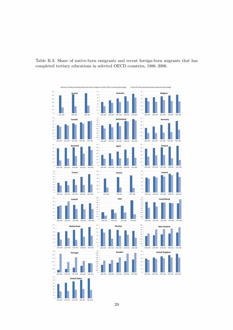
Table B.3: Share of native-born emigrants and recent foreign-born migrants that hascompleted tertiary educations in selected OECD countries, 1986–2006.

0

0.1

0.2

0.3

0.4

0.5

0.6

1994-1998 1998-2002 2002-2006

Austria

0

0.1

0.2

0.3

0.4

0.5

0.6

0.7

1986-1990 1990-1994 1994-1998 1998-2002 2002-2006

Australia

0

0.1

0.2

0.3

0.4

0.5

0.6

1986-1990 1990-1994 1994-1998 1998-2002 2002-2006

Belgium

0

0.1

0.2

0.3

0.4

0.5

0.6

0.7

1986-1990 1990-1994 1994-1998 1998-2002 2002-2006

Canada

0

0.05

0.1

0.15

0.2

0.25

0.3

0.35

0.4

0.45

0.5

1986-1990 1990-1994 1994-1998 1998-2002 2002-2006

Switzerland

0

0.1

0.2

0.3

0.4

0.5

0.6

1986-1990 1990-1994 1994-1998 1998-2002 2002-2006

Germany

0

0.1

0.2

0.3

0.4

0.5

0.6

1986-1990 1990-1994 1994-1998 1998-2002 2002-2006

Denmark

0

0.1

0.2

0.3

0.4

0.5

0.6

0.7

1986-1990 1990-1994 1994-1998 1998-2002 2002-2006

Spain

0

0.1

0.2

0.3

0.4

0.5

0.6

1986-1990 1990-1994 1994-1998 1998-2002 2002-2006

Finland

0

0.1

0.2

0.3

0.4

0.5

0.6

0.7

0.8

1986-1990 1990-1994 1994-1998 1998-2002 2002-2006

France

0

0.1

0.2

0.3

0.4

0.5

0.6

1994-1998 1998-2002 2002-2006

Greece

0

0.1

0.2

0.3

0.4

0.5

0.6

1986-1990 1990-1994 1994-1998 1998-2002 2002-2006

Ireland

0

0.1

0.2

0.3

0.4

0.5

0.6

1986-1990 1990-1994 1994-1998 1998-2002 2002-2006

Iceland

0

0.05

0.1

0.15

0.2

0.25

0.3

0.35

0.4

0.45

1986-1990 1990-1994 1994-1998 1998-2002

Italy

0

0.05

0.1

0.15

0.2

0.25

0.3

0.35

0.4

0.45

0.5

1986-1990 1990-1994 1994-1998 1998-2002 2002-2006

Luxembourg

0

0.1

0.2

0.3

0.4

0.5

0.6

1986-1990 1990-1994 1994-1998 1998-2002 2002-2006

Netherlands

0

0.1

0.2

0.3

0.4

0.5

0.6

1986-1990 1990-1994 1994-1998 1998-2002 2002-2006

Norway

0

0.05

0.1

0.15

0.2

0.25

0.3

0.35

0.4

0.45

1986-1990 1990-1994 1994-1998 1998-2002 2002-2006

New Zealand

0

0.05

0.1

0.15

0.2

0.25

0.3

1986-1990 1990-1994 1994-1998 1998-2002 2002-2006

Portugal

0

0.05

0.1

0.15

0.2

0.25

0.3

0.35

0.4

0.45

0.5

1986-1990 1990-1994 1994-1998 1998-2002 2002-2006

Sweden

0

0.1

0.2

0.3

0.4

0.5

0.6

1986-1990 1990-1994 1994-1998 1998-2002 2002-2006

United Kingdom

0

0.1

0.2

0.3

0.4

0.5

0.6

0.7

1986-1990 1990-1994 1994-1998 1998-2002 2002-2006

United States

0

2share of tertiary educated among native born emigrants to other OECD countries (percentage) share of teriary educated among immigrants (percentage)

29

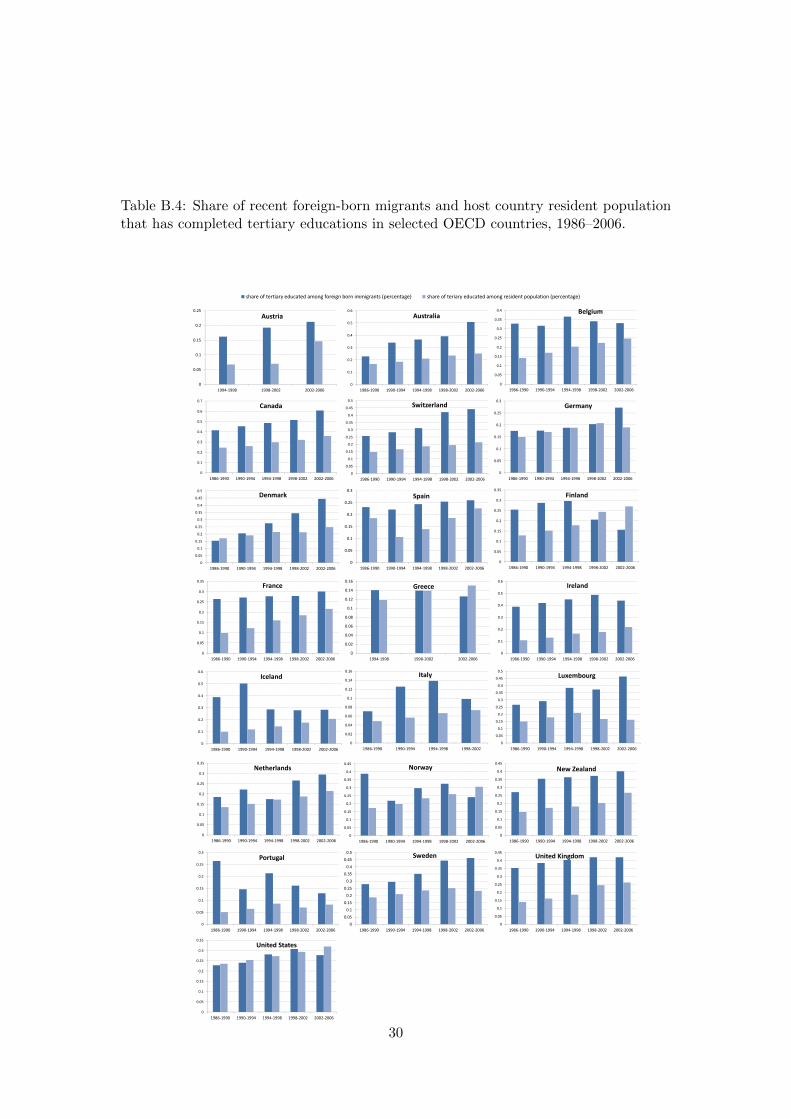
Table B.4: Share of recent foreign-born migrants and host country resident populationthat has completed tertiary educations in selected OECD countries, 1986–2006.

0

0.05

0.1

0.15

0.2

0.25

1994-1998 1998-2002 2002-2006

Austria

0

0.1

0.2

0.3

0.4

0.5

0.6

1986-1990 1990-1994 1994-1998 1998-2002 2002-2006

Australia

0

0.05

0.1

0.15

0.2

0.25

0.3

0.35

0.4

1986-1990 1990-1994 1994-1998 1998-2002 2002-2006

Belgium

0

0.1

0.2

0.3

0.4

0.5

0.6

0.7

1986-1990 1990-1994 1994-1998 1998-2002 2002-2006

Canada

0

0.05

0.1

0.15

0.2

0.25

0.3

0.35

0.4

0.45

0.5

1986-1990 1990-1994 1994-1998 1998-2002 2002-2006

Switzerland

0

0.05

0.1

0.15

0.2

0.25

0.3

1986-1990 1990-1994 1994-1998 1998-2002 2002-2006

Germany

0

0.05

0.1

0.15

0.2

0.25

0.3

0.35

0.4

0.45

0.5

1986-1990 1990-1994 1994-1998 1998-2002 2002-2006

Denmark

0

0.05

0.1

0.15

0.2

0.25

0.3

1986-1990 1990-1994 1994-1998 1998-2002 2002-2006

Spain

0

0.05

0.1

0.15

0.2

0.25

0.3

0.35

1986-1990 1990-1994 1994-1998 1998-2002 2002-2006

Finland

0

0.05

0.1

0.15

0.2

0.25

0.3

0.35

1986-1990 1990-1994 1994-1998 1998-2002 2002-2006

France

0

0.02

0.04

0.06

0.08

0.1

0.12

0.14

0.16

1994-1998 1998-2002 2002-2006

Greece

0

0.1

0.2

0.3

0.4

0.5

0.6

1986-1990 1990-1994 1994-1998 1998-2002 2002-2006

Ireland

0

0.1

0.2

0.3

0.4

0.5

0.6

1986-1990 1990-1994 1994-1998 1998-2002 2002-2006

Iceland

0

0.02

0.04

0.06

0.08

0.1

0.12

0.14

0.16

1986-1990 1990-1994 1994-1998 1998-2002

Italy

0

0.05

0.1

0.15

0.2

0.25

0.3

0.35

0.4

0.45

0.5

1986-1990 1990-1994 1994-1998 1998-2002 2002-2006

Luxembourg

0

0.05

0.1

0.15

0.2

0.25

0.3

0.35

1986-1990 1990-1994 1994-1998 1998-2002 2002-2006

Netherlands

0

0.05

0.1

0.15

0.2

0.25

0.3

0.35

0.4

0.45

1986-1990 1990-1994 1994-1998 1998-2002 2002-2006

Norway

0

0.05

0.1

0.15

0.2

0.25

0.3

0.35

0.4

0.45

1986-1990 1990-1994 1994-1998 1998-2002 2002-2006

New Zealand

0

0.05

0.1

0.15

0.2

0.25

0.3

1986-1990 1990-1994 1994-1998 1998-2002 2002-2006

Portugal

0

0.05

0.1

0.15

0.2

0.25

0.3

0.35

0.4

0.45

0.5

1986-1990 1990-1994 1994-1998 1998-2002 2002-2006

Sweden

0

0.05

0.1

0.15

0.2

0.25

0.3

0.35

0.4

0.45

1986-1990 1990-1994 1994-1998 1998-2002 2002-2006

United Kingdom

0

0.05

0.1

0.15

0.2

0.25

0.3

0.35

1986-1990 1990-1994 1994-1998 1998-2002 2002-2006

United States

0

2

share of tertiary educated among foreign born immigrants (percentage) share of teriary educated among resident population (percentage)

30

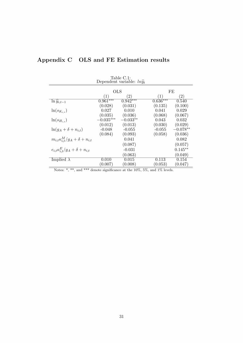
Appendix C OLS and FE Estimation results

Table C.1:Dependent variable: lnyt

OLS FE(1) (2) (1) (2)

ln yi,t−1 0.961∗∗∗ 0.942∗∗∗ 0.636∗∗∗ 0.540(0.028) (0.031) (0.135) (0.100)

ln(sKi,t) 0.027 0.010 0.041 0.029

(0.035) (0.036) (0.068) (0.067)ln(sHi,t

) −0.035∗∗∗ −0.033∗∗ 0.043 0.032(0.012) (0.013) (0.030) (0.029)

ln(gA + δ + ni,t) -0.048 -0.055 -0.055 −0.078∗∗

(0.084) (0.093) (0.058) (0.036)mi,tκ

Mi,t/gA + δ + ni,t 0.041 0.082

(0.087) (0.057)ei,tκ

Ei,t/gA + δ + ni,t -0.031 0.145∗∗

(0.063) (0.049)Implied λ 0.010 0.015 0.113 0.154

(0.007) (0.008) (0.053) (0.047)

Notes: *, **, and *** denote significance at the 10%, 5%, and 1% levels.

31

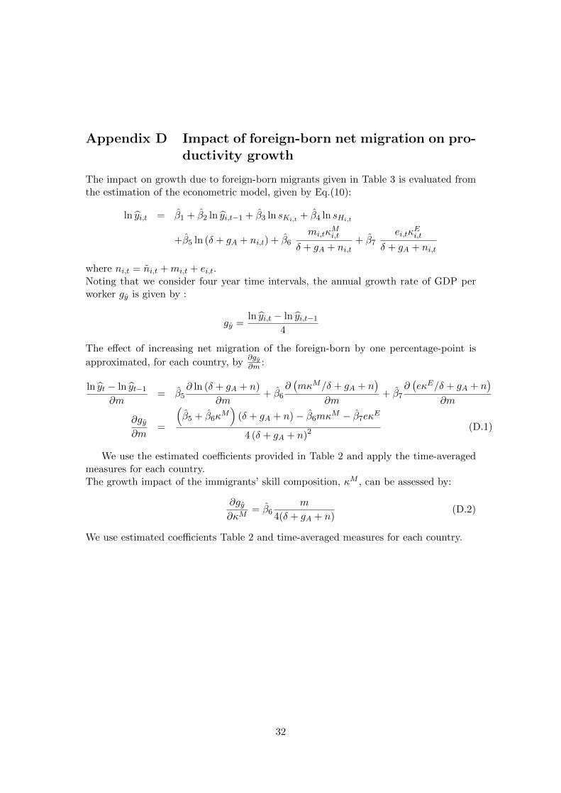
Appendix D Impact of foreign-born net migration on pro-ductivity growth

The impact on growth due to foreign-born migrants given in Table 3 is evaluated fromthe estimation of the econometric model, given by Eq.(10):

ln yi,t = β1 + β2 ln yi,t−1 + β3 ln sKi,t + β4 ln sHi,t

+β5 ln (δ + gA + ni,t) + β6mi,tκ

Mi,t

δ + gA + ni,t+ β7

ei,tκEi,t

δ + gA + ni,t

where ni,t = ni,t +mi,t + ei,t.Noting that we consider four year time intervals, the annual growth rate of GDP perworker gy is given by :

gy =ln yi,t − ln yi,t−1

4

The effect of increasing net migration of the foreign-born by one percentage-point is

approximated, for each country, by∂gy∂m :

ln yt − ln yt−1

∂m= β5

∂ ln (δ + gA + n)

∂m+ β6

∂(mκM/δ + gA + n

)∂m

+ β7∂(eκE/δ + gA + n

)∂m

∂gy∂m

=

(β5 + β6κ

M)

(δ + gA + n)− β6mκM − β7eκE

4 (δ + gA + n)2(D.1)

We use the estimated coefficients provided in Table 2 and apply the time-averagedmeasures for each country.The growth impact of the immigrants’ skill composition, κM , can be assessed by:

∂gy∂κM

= β6m

4(δ + gA + n)(D.2)

We use estimated coefficients Table 2 and time-averaged measures for each country.

32

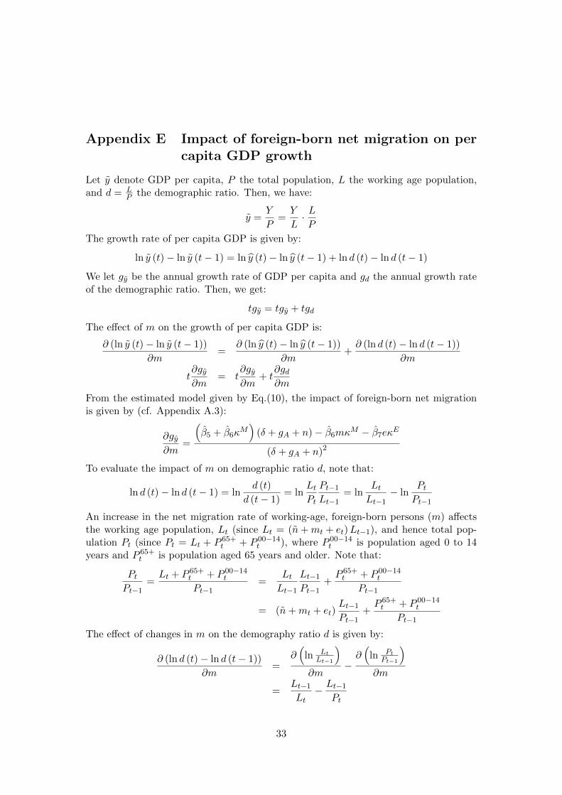
Appendix E Impact of foreign-born net migration on percapita GDP growth

Let y denote GDP per capita, P the total population, L the working age population,and d = L

P the demographic ratio. Then, we have:

y =Y

P=Y

L· LP

The growth rate of per capita GDP is given by:

ln y (t)− ln y (t− 1) = ln y (t)− ln y (t− 1) + ln d (t)− ln d (t− 1)

We let gy be the annual growth rate of GDP per capita and gd the annual growth rateof the demographic ratio. Then, we get:

tgy = tgy + tgd

The effect of m on the growth of per capita GDP is:

∂ (ln y (t)− ln y (t− 1))

∂m=

∂ (ln y (t)− ln y (t− 1))

∂m+∂ (ln d (t)− ln d (t− 1))

∂m

t∂gy∂m

= t∂gy∂m

+ t∂gd∂m

From the estimated model given by Eq.(10), the impact of foreign-born net migrationis given by (cf. Appendix A.3):

∂gy∂m

=

(β5 + β6κ

M)

(δ + gA + n)− β6mκM − β7eκE

(δ + gA + n)2

To evaluate the impact of m on demographic ratio d, note that:

ln d (t)− ln d (t− 1) = lnd (t)

d (t− 1)= ln

LtPt

Pt−1

Lt−1= ln

LtLt−1

− lnPtPt−1

An increase in the net migration rate of working-age, foreign-born persons (m) affectsthe working age population, Lt (since Lt = (n+mt + et)Lt−1), and hence total pop-ulation Pt (since Pt = Lt + P 65+

t + P 00−14t ), where P 00−14

t is population aged 0 to 14years and P 65+

t is population aged 65 years and older. Note that:

PtPt−1

=Lt + P 65+

t + P 00−14t

Pt−1=

LtLt−1

Lt−1

Pt−1+P 65+t + P 00−14

t

Pt−1

= (n+mt + et)Lt−1

Pt−1+P 65+t + P 00−14

t

Pt−1

The effect of changes in m on the demography ratio d is given by:

∂ (ln d (t)− ln d (t− 1))

∂m=

∂(

ln LtLt−1

)∂m

−∂(

ln PtPt−1

)∂m

=Lt−1

Lt− Lt−1

Pt

33

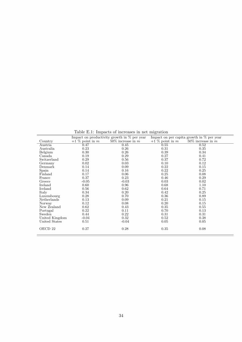
Table E.1: Impacts of increases in net migrationImpact on productivity growth in % per year Impact on per capita growth in % per year

Country +1 % point in m 50% increase in m +1 % point in m 50% increase in mAustria 0.47 0.45 0.55 0.52Australia 0.23 0.26 0.31 0.35Belgium 0.30 0.26 0.39 0.34Canada 0.19 0.29 0.27 0.41Switzerland 0.29 0.56 0.37 0.72Germany 0.02 0.03 0.10 0.12Denmark 0.14 0.09 0.22 0.15Spain 0.14 0.16 0.22 0.25Finland 0.17 0.06 0.25 0.08France 0.37 0.23 0.46 0.29Greece -0.05 -0.03 0.03 0.02Ireland 0.60 0.96 0.68 1.10Iceland 0.56 0.62 0.64 0.71Italy 0.34 0.20 0.42 0.25Luxembourg 0.28 0.70 0.36 0.89Netherlands 0.13 0.09 0.21 0.15Norway 0.12 0.08 0.20 0.15New Zealand 0.62 0.43 0.35 0.55Portugal 0.22 0.11 0.70 0.13Sweden 0.44 0.22 0.31 0.31United Kingdom -0.04 0.32 0.52 0.38United States 0.51 -0.04 0.05 0.05

OECD 22 0.27 0.28 0.35 0.08

34