DOCTORAL THESIS - oa.upm.esoa.upm.es/373/1/ELENA_LOPEZ_SUAREZ.pdf · sus siempre acertados...
304
UNIVERSIDAD POLITÉCNICA DE MADRID ESCUELA TÉCNICA SUPERIOR DE INGENIEROS DE CAMINOS, CANALES Y PUERTOS ASSESSMENT OF TRANSPORT INFRASTRUCTURE PLANS: A STRATEGIC APPROACH INTEGRATING EFFICIENCY, COHESION AND ENVIRONMENTAL ASPECTS DOCTORAL THESIS Elena López Suárez Ingeniero de Caminos, Canales y Puertos Madrid, 2007
Transcript of DOCTORAL THESIS - oa.upm.esoa.upm.es/373/1/ELENA_LOPEZ_SUAREZ.pdf · sus siempre acertados...

UNIVERSIDAD POLITÉCNICA DE MADRID ESCUELA TÉCNICA SUPERIOR
DE INGENIEROS DE CAMINOS, CANALES Y PUERTOS
ASSESSMENT OF TRANSPORT INFRASTRUCTURE PLANS: A STRATEGIC APPROACH INTEGRATING EFFICIENCY, COHESION AND ENVIRONMENTAL
ASPECTS
DOCTORAL THESIS
Elena López Suárez Ingeniero de Caminos, Canales y Puertos
Madrid, 2007


DEPARTAMENTO DE INGENIERÍA CIVIL: TRANSPORTES
Escuela Técnica Superior de Ingenieros de Caminos, Canales y Puertos
ASSESSMENT OF TRANSPORT INFRASTRUCTURE PLANS: A STRATEGIC APPROACH INTEGRATING EFFICIENCY,
COHESION AND ENVIRONMENTAL ASPECTS
DOCTORAL THESIS
Elena López Suárez Ingeniero de Caminos, Canales y Puertos
Director:
Andrés Monzón de Cáceres Dr. Ingeniero de Caminos, Canales y Puertos
Madrid, 2007


Tribunal nombrado por el Mgfco. y Excmo. Sr. Rector de la Universidad Politécnica de Madrid, el día ___ de _______________ de 2007.
Presidente: _____________________________________________ Vocal: _____________________________________________ Vocal: _____________________________________________ Vocal: _____________________________________________ Secretario: _____________________________________________ Realizado el acto de defensa y lectura de la Tesis el día ___ de _______________ de 2007 en la E.T.S. de Ingenieros de Caminos, Canales y Puertos de la U.P.M. Calificación: ______________________________ EL PRESIDENTE LOS VOCALES
EL SECRETARIO


A mis padres, Micaela y Sebastián,
mis raíces, mis maestros
‘El hombre, en su centro, es siempre potencialmente
un hombre docto, un sabio y un maestro’
KALFRIED DÜRCKHEIM


ABSTRACT
During the last few decades there has been a shift in transport planning objectives
from economic efficiency towards strategic policy goals, such as cohesion or
environmental issues, intimately linked with the ‘sustainable transport’ paradigm.
However, the treatment of these strategic aspects is uneven and scarce among
assessment methodologies. The development of harmonized methodologies for the
strategic assessment of large scale transport infrastructure investments, such as
transport infrastructure Plans, is therefore a current challenge for the research
community.
This doctoral thesis addresses this challenge by presenting a methodology for the
assessment of transport infrastructure Plans. The proposed methodology
constitutes a strategic approach, based on the utilisation of spatial impact analysis
tools supported by a Geographical Information System (GIS). The assessment
criteria, based on the ‘sustainable transport’ paradigm, are structured into
efficiency, cohesion and environmental criteria. The procedure selected for the
integration of the assessment criteria results follows a multicriteria analysis
approach.
The suggested methodology defines a comprehensive technical procedure for the
assessment of strategic effects of transport infrastructure Plans, which is believed
to constitute a useful, transparent and flexible planning tool both for planners and
decision-makers.
The validity of the methodology is tested with its application to a case study: the
Spanish Strategic Transport and Infrastructure Plan 2005-2020 (PEIT).

RESUMEN
En las últimas décadas se viene produciendo un cambio en los objetivos que dirigen
las labores de planificación de infraestructuras de transporte, desde la eficiencia
económica hacia objetivos de carácter más estratégico, como la cohesión o los
aspectos medioambientales. Sin embargo, no existe un consenso sobre la forma en
que se deben incluir estos aspectos estratégicos en las metodologías de evaluación
oficiales, sobre todo en las que se refieren a inversiones a gran escala, como es el
caso de los Planes de infraestructura de transporte.
Esta tesis doctoral avanza en esta línea de investigación mediante la propuesta de
una metodología para la evaluación de Planes de infraestructura de transporte. La
metodología sigue un enfoque estratégico, basado en la utilización de herramientas
de análisis territorial aplicadas sobre un soporte SIG (Sistema de Información
Geográfica). Los objetivos de evaluación, basados en el paradigma del ‘transporte
sostenible’, se han estructurado en torno a criterios de eficiencia, cohesión y
medioambientales. Para su integración se ha seleccionado un método de evaluación
multicriterio.
La metodología propuesta define un procedimiento de evaluación que constituye
una herramienta útil en las labores de planificación de infraestructuras, permitiendo
la interacción entre planificadores como para decisores, así como un instrumento de
apoyo para la comunicación de resultados a la opinión pública, gracias a la cuidada
representación gráfica de resultados.
La validez de la metodología ha sido comprobada mediante su aplicación a un caso
de estudio: el Plan Estratégico de Infraestructuras y Transporte 2005-2020 (PEIT)
español.

ACKNOWLEDGMENTS
I would like to start by thanking Andrés Monzón, my thesis supervisor, for the
valuable and constant support he has given me these past four years. His
confidence in my work during difficult times has been very important help for me to
finish the thesis and my studies.
From the Transport Department and from TRANSyT-UPM I would like to thank the
teaching staff, especially Rafael Izquierdo, Aniceto Zaragoza, Oscar Martínez, José
Manuel Vassallo and the Transport Department Director, Miguel Ángel del Val. They
have all encouraged me and shared their experience with me from the first day at
the University. I also want to thank Javier Gutiérrez Puebla, from UCM, for his wise
comments and suggestions, which have served me as an invaluable guide during
the development of the research work. I also would like to thank Lawrence Baron
for his meticulous work in editing my thesis without loosing his enthusiasm and
smile.
My colleagues at TRANSyT-UPM have been there when I needed them, day after
day. Firstly, I want to thank Emilio Ortega and Belén Martín for their help in the
preparation of the maps and Santiago Mancebo for his wise comments. I also want
to specially thank Paula Vieira, Rocío Cascajo, Esther Madrigal, Mª Eugenia López,
Ana María Pardeiro, Paul Pffafenbichler, Daniel de la Hoz and Carmen Pérez. Thank
you for all the help you have given me.
Many other people have given me their support during my weak moments; I am
very lucky to have been able to depend on them during all this time. Thanks are
due to Manuel, Concha. Fernando, Cristina, Pepe, Pilar, Jose, Miren, Marta, Marieta,
Sara, Patricia, and many others: thank you for the right words and the good
gestures.
Finally, a big GRACIAS to my family. To my grandparents, Rosa and Eugenio, who
have given me serenity when I needed it most. To my brother Chano, thanks for
your advice, mi niño! And of course, to my parents, Micaela and Sebastián, for
teaching me how to get the best of myself. Thank you for showing me so much
love. For being there. Always.

AGRADECIMIENTOS
En primer lugar, quiero agradecer a mi Director de tesis, Andrés Monzón, el
respaldo decidido y constante que me ha ofrecido durante estos años. Su apuesta
por mi trabajo en los momentos difíciles ha sido muy importante para que haya
podido terminar esta tesis.
Quiero expresar también mi agradecimiento al Departamento de Transportes y a
TRANSyT-UPM, en particular a Rafael Izquierdo, Aniceto Zaragoza, Oscar Martínez y
José Manuel Vassallo, y al Director del Departamento, Miguel Ángel del Val. Todos
ellos me han infundo ánimos y me han aconsejado desde el primer día, desde la
serenidad de su experiencia. Quiero agradecer también a Javier Gutiérrez Puebla
sus siempre acertados comentarios y sugerencias, que me han servido de
inestimable guía durante el desarrollo de la investigación. Debo agradecer también
a Lawrence Baron el haberse encargado de la minuciosa tarea de edición del inglés
del texto, sin perder nunca el entusiasmo ni la sonrisa.
Mis compañeros de TRANSyT-UPM son los que me han acompañado en el día a día.
En primer lugar quiero agradecer a Emilio Ortega y a Belén Martín su gran ayuda en
la elaboración de los mapas y a Santiago Mancebo sus certeros comentarios. Quiero
dar las gracias de forma especial a Paula Vieira, Rocío Cascajo, Esther Madrigal, Mª
Eugenia López, Ana María Pardeiro, Paul Pffafenbichler, Daniel de la Hoz y Carmen
Pérez. Compañeros, gracias a todos por el enorme cariño que me han demostrado
en este tiempo.
He tenido la suerte de contar con gente que me ha dado aliento cuando me fallaban
las fuerzas. Gracias a Manuel y a Concha, maestros en el camino. Fernando,
Cristina, Pepe, Pilar, Jose, Miren, Marta, Marieta, Sara, Patricia, y tantos otros:
gracias por ayudarme con la palabra y el gesto apropiados en cada momento.
Por último, un GRACIAS a mi familia. A mis abuelos Rosa y Eugenio, que me han
dado serenidad cuando más la he necesitado. A mi hermano Chano: gracias por tus
consejos, mi niño!. Y por supuesto, a mis padres, Micaela y Sebastián, por
enseñarme a dar lo mejor de mí misma. Gracias por demostrarme tanto amor. Por
estar ahí. Siempre.

TABLE OF CONTENTS
-vii-
TABLE OF CONTENTS
DEDICATION……………………………………………………………………………………….i
ABSTRACT………………………………………………………………………………………...iii
ACKNOWLEDGMENTS………………………………………………………………………….v
CONTENTS……………………………………………………………………………………….vii
LIST OF TABLES..……………………………………………………………………………….x
LIST OF FIGURES………………………………………………………………………………xi
LIST OF ABBREVIATIONS…………………………………………………………………..xv
CONTENTS
1. INTRODUCTION ........................................................................ 1
1.1 Problem statement ................................................................... 1
1.2 Objectives................................................................................. 3
1.3 Research methodology.............................................................. 3
1.4 Structure of the thesis .............................................................. 5
2. A CHANGING PLANNING FRAMEWORK...................................... 7
2.1 Introduction.............................................................................. 7
2.2 Structuring the planning process .............................................. 9
2.2.1 Sources of conflicts in objective setting........................................... 9
2.2.2 A guiding principle: the sustainable development approach ............... 9
2.2.3 EU policy objectives ....................................................................13
2.3 The evaluation approach......................................................... 16
2.3.1 Introduction ...............................................................................16
2.3.2 Outline of an evaluation process ...................................................17
2.3.3 Current state of the practice in Europe ..........................................22
2.4 The role of evaluation in decision-making............................... 30
2.5 Conclusions............................................................................. 33
3. SPATIAL IMPACT ANALYSIS TOOLS ........................................ 35
3.1 Spatial impacts at the Plan level ............................................. 35
3.1.1 Theoretical foundations of spatial impact analysis ...........................35

TABLE OF CONTENTS
-viii-
3.1.2 Impact analysis at the Plan level...................................................36
3.1.3 The treatment of wider policy impacts at the Plan level....................38
3.2 The potential of accessibility analysis..................................... 43
3.2.1 The concept of accessibility ..........................................................43
3.2.2 The measurement of accessibility .................................................45
3.2.3 Applications in transport planning .................................................53
3.3 Spatial impact and GIS ........................................................... 61
3.3.1 GIS background..........................................................................61
3.3.2 Applications of GIS in transport planning .......................................63
3.4 Conclusions ............................................................................ 66
4. METHODOLOGY FOR THE ASSESSMENT OF TRANSPORT
INFRASTRUCTURE PLANS ....................................................... 69
4.1 Structure of the methodology ................................................. 69
4.2 Definition of the assessment framework ................................ 71
4.2.1 Assessment time horizon .............................................................71
4.2.2 Delimitation of the study area ......................................................72
4.3 Definition of assessment criteria ............................................ 72
4.3.1 Efficiency ...................................................................................73
4.3.2 Cohesion ...................................................................................73
4.3.3 Environmental sustainability.........................................................74
4.4 Definition of performance indicators ...................................... 75
4.4.1 Efficiency ...................................................................................76
4.4.2 Cohesion ...................................................................................78
4.4.3 Environmental sustainability.........................................................81
4.5 Integration ............................................................................. 84
4.5.1 Outline of the proposed approach .................................................84
4.5.2 Weight estimation.......................................................................85
4.5.3 Utility functions ..........................................................................86
4.6 Sensitivity analysis ................................................................. 86
4.6.1 Weight sensitivity .......................................................................87
4.6.2 Attribute value sensitivity ............................................................87
5. CASE STUDY DESCRIPTION..................................................... 87
5.1 Introduction ........................................................................... 87
5.2 Case study characterization.................................................... 88
5.2.1 The surface transport infrastructure networks ................................89
5.2.2 The socio-economic system..........................................................90
5.2.3 Current challenges of the Spanish transport system ........................95

TABLE OF CONTENTS
-ix-
5.2.4 The Strategic Infrastructure and Transport Plan 2005-2020
(PEIT) .....................................................................................100
5.3 The assessment framework .................................................. 101
5.3.1 Assessment time horizon and delimitation of the study area...........101
5.3.2 Definition of alternatives............................................................101
5.3.3 Generation of the GIS database..................................................104
6. ASSESSMENT RESULTS.......................................................... 111
6.1 Efficiency .............................................................................. 111
6.1.1 Network efficiency (NE) .............................................................111
6.1.2 Cross-border integration (CB).....................................................121
6.2 Cohesion ............................................................................... 129
6.2.1 Regional cohesion (RC)..............................................................129
6.2.2 Social cohesion (SC) .................................................................140
6.3 Environmental sustainability ................................................ 149
6.3.1 Global warming (GW) ................................................................149
6.3.2 Habitat fragmentation (HF) ........................................................153
6.4 Discussion on performance indicator results ........................ 156
6.4.1 Road mode ..............................................................................156
6.4.2 Rail mode ................................................................................158
6.5 Integration of results............................................................ 159
6.5.1 Description of the simplified integration procedure ........................159
6.5.2 Road mode ..............................................................................160
6.5.3 Rail mode ................................................................................162
6.5.4 Sensitivity analysis....................................................................164
7. CONCLUSIONS, CONTRIBUTIONS AND FUTURE RESEARCH ... 169
7.1 Conclusions........................................................................... 169
7.1.1 Literature review ......................................................................169
7.1.2 Methodological approach............................................................170
7.1.3 Case study application...............................................................171
7.1.4 Recommendations from a transport planning perspective...............173
7.2 Contributions ........................................................................ 175
7.3 Recommendations for future research .................................. 176
8. REFERENCES ......................................................................... 179
APPENDICES:
APPENDIX A: DEFINITION OF CRITERIA WEIGHTS…………………………..............……205
APPENDIX B: CASE STUDY APPLICATION OF THE ACCESSIBILITY MODEL…………209

TABLE OF CONTENTS
-x-
LIST OF TABLES
Table 2.1: Consideration of TEN-T territorial goals suggested in the UTS study ....26
Table 2.2: Accessibility categories (left) and evaluation matrix for distribution and
development objectives (right) of the German procedure ............................29
Table 4.1: Assessment criteria .......................................................................73
Table 4.2: Assessment criteria and performance indicators ................................76
Table 4.3: Weighting factor matrix for the cohesion criterion .............................80
Table 4.4: Structural backwardness categories.................................................80
Table 4.5: Accessibility analysis categories ......................................................80
Table 4.6: Example of the computation of PARA values .....................................83
Table 4.7: Matrix for scenario building ............................................................88
Table 5.1: Spanish administrative divisions and their NUTS correspondence ........91
Table 6.1 Network efficiency in Spanish NUTS-3 capitals. Road mode................115
Table 6.2 Network efficiency in Spanish NUTS-3 capitals. Rail mode .................120
Table 6.3: Network efficiency in Portuguese district capitals. Road mode ...........123
Table 6.4: Network efficiency in French department capitals. Road mode ..........125
Table 6.5 Network efficiency in Portuguese district capitals. Rail mode ..............127
Table 6.6: Network efficiency in French department capitals. Rail mode ............128
Table 6.7: Regional inequality indices. Road accessibility.................................133
Table 6.8: Regional cohesion performance indicator (RC). Road accessibility......134
Table 6.9: Regional inequality indices. Rail accessibility...................................138
Table 6.10: Regional cohesion performance indicator (RC). Rail accessibility ......139
Table 6.11 Travel time savings and estimated induced traffic ...........................151
Table 6.12: Forecasted induced traffic and corresponding increases in GHG
emissions. Do-nothing vs. PEIT alternative. Road and rail modes ...............152
Table 6.13 Summary of performance indicator values. Road mode ...................157
Table 6.14 Summary of performance indicator values. Rail mode .....................158
Table 6.15: Definition of value functions. Road mode ......................................160
Table 6.16: Integration of results. A0 vs. APEIT. Road mode ..............................162
Table 6.17: Definition of value functions. Rail mode........................................163
Table 6.18: Integration of results. A0 vs. APEIT. Rail mode ................................163

TABLE OF CONTENTS
-xi-
LIST OF FIGURES
Figure 2.1: The planning process ..................................................................... 7
Figure 2.2: Trade-off approach to sustainable transport ....................................13
Figure 2.3: Outline structure of the German spatial impact assessment module....28
Figure 2.4: Considerations affecting the decision-making process .......................31
Figure 3.1: Simple representation of a spatial impact system .............................36
Figure 3.2: Suggested twin approach to transport appraisal ...............................39
Figure 3.3: Activity and impedance functions ...................................................46
Figure 3.4: Example of a travel cost indicator. Road accessibility 1992 ................48
Figure 3.5: Network efficiency. Road accessibility 2005 (left) and 2020 (right) .....49
Figure 3.6: Daily accessibility indicator. Daily accessibility by rail (1993) .............51
Figure 3.7: Outline of the SASI model .............................................................57
Figure 3.8: Changes in GDP per capita as a result of the planned TEN priority
projects.................................................................................................58
Figure 3.9: Superposition of data layers in GIS for a transport study...................62
Figure 3.10: An integrated GIS approach to accessibility analysis. ......................65
Figure 4.1: Structure of the methodology ........................................................70
Figure 4.2: Comparison of alternatives ............................................................71
Figure 4.3: Performance indicators’ inputs .......................................................75
Figure 4.4. Scheme of the calculation of the PARA index....................................83
Figure 4.5: The integration procedure .............................................................85
Figure 5.1. Spanish road network (2005).........................................................89
Figure 5.2. Spanish rail network (2005)...........................................................90
Figure 5.3: Spanish NUTS divisions.................................................................91
Figure 5.4: Population density........................................................................92
Figure 5.5: Study area system of cities ...........................................................93
Figure 5.6: Growth in GDP per head in Spain, Spanish NUTS-2 regions and EU15 in
terms of EU25 average (PPS) 1995-2003...................................................94
Figure 5.7: Trends in GDP per head in Spanish NUTS-2 regions, EU15 and EU25 in
terms of Spain’ average, 1995-2003 .........................................................95
Figure 5.8: Accessibility by road (2005) ..........................................................96
Figure 5.9: Accessibility by rail (2005) ............................................................97
Figure 5.10: Trends in mobility, GDP and emissions in Spain, 1990-2003 ............99
Figure 5.11: Delimitation of the study area ....................................................102
Figure 5.12: Road network of the PEIT alternative (APEIT).................................103

TABLE OF CONTENTS
-xii-
Figure 5.13: Rail network of the PEIT alternative (APEIT) ..................................103
Figure 5.14: Sites of Community importance (SCIs) .......................................107
Figure 5.15: Special Protection Areas (SPAs) .................................................108
Figure 5.16: Spanish habitats map ...............................................................109
Figure 6.1: Network efficiency. Alternative A0. Road mode...............................112
Figure 6.2: Network efficiency. Alternative APEIT. Road mode............................114
Figure 6.3: Network efficiency. Relative differences Alternative A0 vs. APEIT. Road
mode ..................................................................................................114
Figure 6.4: Network accessibility. Alternative A0. Rail mode .............................117
Figure 6.5: Network accessibility. Alternative APEIT. Rail mode ..........................119
Figure 6.6: Network accessibility. Relative differences Alternative A0 vs. APEIT. Rail
mode ..................................................................................................119
Figure 6.7: Network efficiency in Portugal. Relative differences Alternative A0 vs.
APEIT. Road mode ..................................................................................122
Figure 6.8: Network efficiency in Southern France. Relative differences Alternative
A0 vs. APEIT. Road mode.........................................................................124
Figure 6.9: Network efficiency in Portugal. Relative differences Alternative A0 vs.
APEIT. Rail mode....................................................................................126
Figure 6.10: Network efficiency in Southern France. Relative differences Alternative
A0 vs. APEIT. Rail mode...........................................................................128
Figure 6.11: Potential accessibility. Alternative A0. Road mode .........................131
Figure 6.12: Box-plot of potential accessibility values in the do-nothing alternative.
NUTS-2 aggregation. Road mode............................................................131
Figure 6.13: Potential accessibility. Alternative APEIT. Road mode ......................132
Figure 6.14: Changes in potential accessibility. Alternative APEIT vs. A0. Road mode
..........................................................................................................133
Figure 6.15: Relative change in road accessibility inequality indices ..................134
Figure 6.16: Potential accessibility. Alternative A0. Rail mode...........................136
Figure 6.17: Box-plot of potential accessibility values in the do-nothing alternative.
NUTS-2 aggregation. Rail mode .............................................................136
Figure 6.18: Potential accessibility. Alternative APEIT. Rail mode........................137
Figure 6.19: Changes in potential accessibility. Alternative APEIT vs. A0. Road mode
..........................................................................................................138
Figure 6.20: Regional cohesion indices. Rail mode ..........................................139
Figure 6.21: NUTS-5 unemployment rates .....................................................140
Figure 6.22: Standardized absolute change of NUTS-5 regions in the potential
accessibility indicator. Road mode ..........................................................142

TABLE OF CONTENTS
-xiii-
Figure 6.23: Standardized relative change of NUTS-5 regions in the potential
accessibility indicator. Road mode ..........................................................142
Figure 6.24: Accessibility categories. Road mode............................................143
Figure 6.25: Structural backwardness categories ............................................144
Figure 6.26: Regional weighting factor. Road mode.........................................144
Figure 6.27: Standardized absolute change of NUTS-5 regions in the potential
accessibility indicator. Rail mode ............................................................146
Figure 6.28: Standardized relative change of NUTS-5 regions in the potential
accessibility indicator. Rail mode ............................................................147
Figure 6.29: Accessibility deficiency categories. Rail mode...............................148
Figure 6.30: Regional weighting factor. Rail mode ..........................................148
Figure 6.31: % change in the PARA index in SCIs. Road mode .........................154
Figure 6.32: % change in the PARA index in SPAs. Road mode.........................154
Figure 6.33: % change in the PARA index in SCIs. Rail mode ...........................155
Figure 6.34: % change in the PARA index in SPAs. Rail mode...........................156
Figure 6.35: Value function for the network efficiency criterion. Road mode.......161
Figure 6.36: Criterion weight sensitivity: efficiency criterion.............................164
Figure 6.37: Criterion weight sensitivity: cohesion criterion .............................165
Figure 6.38: Criterion weight sensitivity: environmental criterion......................165
Figure 6.39: Attribute value sensitivity. Road mode ........................................167

TABLE OF CONTENTS
-xiv-

LIST OF ABBREVIATIONS
-xv-
LIST OF ABBREVIATIONS
AST Appraisal Summary Table
CBA Cost-benefit analysis
CTP Common Transport Policy
DM Decision maker
DSS Decision support system
EC European Commission
ECMT European Conference of Ministers of Transport
ERDF European Regional Development Fund
ESD Environmentally Sustainable Development
ESDP European Spatial Development Perspective
ESPON European Spatial Observatory Network
EU European Union
FP Framework Programme
GDP Gross Domestic Product
GHG Greenhouse Gas
GIS Geographical Information System
HCR High Capacity Road
HSR High Speed Rail
LUTI Land use and transport interaction
MCA Multicriteria analysis
MMSS Member States
NATA New Approach to Appraisal
OJEU Official Journal of the European Union
PEIT Plan Estratégico de Infraestructuras y Transporte
PPS Purchase Power Standard
RTD Research and Technological Development
SACTRA Standing Advisory Committee on Trunk Road Assessment
SCI Site of Community Importance
SPA Special Protection Area
TEN-T Trans- European Transport Networks
TERM Transport and Environment Reporting Mechanisms

TABLE OF CONTENTS
-xvi-

Chapter 1 – INTRODUCTION
- 1 -
1. INTRODUCTION
1.1 Problem statement
The planning process of a transport infrastructure Plan entails a high degree of
complexity. Although during the past few decades there were important advances
in the development of assessment methodologies at the Plan level, today there are
still many issues for which a consensus has not been reached in the transport
research community. There are a number of reasons why the development of
assessment methodologies at the Plan level is still an area where research efforts
are needed.
First, the inclusion of the sustainable development approach (Serageldin,
1996) in transport planning processes caused a shift in transport planning
objectives towards strategic policy goals, such as network efficiency, cohesion or
environmental issues. This structure of strategic objectives is intimately linked with
the increased inclusion of transport sustainability issues (Greene and Wegener,
1997) into the planning framework. This objective shift has been translated into
policy documents by a wide variety of institutions (OECD, 1998; ECMT, 2004; EC,
2004; EC, 1999). Furthermore, it is necessary to broaden the assessment
objectives to include the above strategic impacts at the Plan level, given that the
scope of the projects might result in impacts elsewhere, either in another
transportation field, or in other sectors such as land use, energy or the
environment. Thus, national governments are increasingly demanding the inclusion
of strategic aspects in assessment methodologies (Bristow and Nellthorp, 2000).
However, both the definitions and the subsequent assessment of these strategic
impacts are uneven and scarce among official methodologies (Grant-Muller et al.,
2001).
Second, the increased importance given to consensus building, transparency
and communicative issues of the planning approach (Voogd and Woltjer, 1999)
calls for an adaptation of ‘black-box’ methodologies resulting in a single score for
each alternative, into ‘easy-to-interpret’ ones, providing relevant information on
different strategic policy aspects. It is increasingly acknowledged that the

Assessment of Transport Infrastructure Plans: a strategic approach
- 2 -
objectives of transportation policy cannot be transformed into one or two
performance criteria, but rather that there are different and competing objectives.
Indeed, decision-makers (DMs) are increasingly requiring the assessment
methodology to include relevant information which they can easily interpret, with
an enhanced graphical presentation of results, so they can make consistent
decisions on their part.
Finally, the high relevance of the political component inherent in the
assessment of transport Plans, means that the roles to be played by the technical
and the political assessment are not clear. This issue is reinforced by the frequent
presence of objective setting conflicts between the different administrative levels
(local, regional, national and European) involved in the planning process at the Plan
level (May et al., 2003; Beinat, 1998). Decision-making today is no longer seen as
an intellectual process, but as a socio-political and organizational process, where
the interest has shifted from the quality of the decision towards the quality of
decision-making (Voogd, 1997). In this context, the technical assessment enables
ranking the alternatives in terms of a set of criteria and priorities, thus making the
political decision-making stage feasible, but in no case replacing the DMs
responsibility.
The above reasons have created a need to develop a suitable methodological
basis that explicitly relates transportation policies to strategic impacts by taking
into account a wide variety of strategic aspects in a flexible and transparent way.
Increased computer capacity and the recent development of assessment tools, such
as Geographic Information Systems (GIS) has enabled the upsurge of important
methodological advances in this direction (Fotheringham and Wegener, 2000).
Hence, assessment methodologies are seen as a form of decision support to
DMs, keeping in mind that the technical assessment is important, but finally it is a
political decision ultimately derived from the consideration of a wider set of factors
than the criteria of efficiency of the transport system or the consideration of
environmental impacts (ME&P et al., 2001).
In this context, further research efforts to develop consistent methodologies
capable of assessing the strategic impacts mentioned above in a flexible and
transparent manner are needed. This thesis, ‘Assessment of transport
infrastructure Plans: a strategic approach integrating efficiency, cohesion and
environmental aspects’ is a step forward in this research line, with a proposed
assessment methodology and its subsequent validation in a case study.

Chapter 1 – INTRODUCTION
- 3 -
1.2 Objectives
The overall objective of this thesis is ‘to develop a methodology capable of
complementing traditional assessment methodologies of transport infrastructure
Plans, from a strategic approach, integrating efficiency, cohesion and environmental
aspects’.
The achievement of this overall objective can be split into the following main
objectives:
� To define the set of strategic criteria, namely efficiency, cohesion and
environmental sustainability, that should be evaluated in the assessment of
transport infrastructure Plans,
� to develop a methodology, based on the use of spatial impact analysis tools,
capable of measuring the achievement of each of the criteria above,
� to integrate the results obtained in each assessment criterion in order to
provide an overall vision of the global performance of each alternative,
� to investigate the influence of the different variables present in the
methodology on the final assessment results,
� to provide DMs with policy recommendations on the basis of the contribution
of each alternative to the achievement of the assessment criteria,
� to develop a useful, transparent and flexible transport planning tool, whose
results can be easy to explain to the public.
1.3 Research methodology
In order to achieve the above objectives, the research work has been structured
into the following stages:
� Investigation of recent changes and the current situation of the transport
planning framework at the Plan level, in order to determine which are the
main strategic policy goals that any assessment methodology should handle.
� Review the current state-of-the-art assessment methodologies at strategic
levels, in order to detect possible incoherencies and methodological gaps.
� Analysis of the potential of spatial impact analysis tools, in particular GIS,
for the development of assessment methodologies and as a support system
in the planning process.
� Justification of the usefulness of accessibility indicators as a planning tool
capable of assessing strategic aspects, such as network efficiency or
cohesion impacts.

Assessment of Transport Infrastructure Plans: a strategic approach
- 4 -
� Definition of a set of strategic criteria and subcriteria that should be included
in the assessment of transport infrastructure Plans, and the corresponding
procedure to assess each one of them.
� Development of a procedure, based on multicriteria analysis (MCA) capable
of ranking a set of alternatives on the basis of their performance on the set
of defined criteria.
� Test of the validity and consistency of the proposed approach through its
application in a case study. The case study corresponds to the Spanish
Strategic Transport and Infrastructure Plan 2005-2020 (PEIT), recently
launched in Spain (Ministerio de Fomento, 2005).
� Drawing of conclusions on the validity of the methodology and identification
of areas for future research.
An important part of the research work developed in this thesis is based on the
findings of different research projects which were developed during the period the
research was carried out (2002-2007). In these projects different strategic impacts
of large scale transport infrastructure investments were assessed. These are listed
below:
� Assessment of territorial impacts of transport infrastructure investments.
Application: analysis of the Spanish transport network. Research Project
funded by the 2002 Ministry of Public Works Research Programme.
� Assessment of the effects of transport infrastructure Plans on mobility, the
territory and the socio-economic system, in the context of the enlargement
of the European Union. Research project funded by the 2004/2007 Ministry
of Science and Technology Research, Development and Innovation
Programme.
� Indicators of impacts of transport infrastructure on social and territorial
equity. Supported by the 2004 Transport research aids of the Ministry of
Public Works Research Programme.

Chapter 1 – INTRODUCTION
- 5 -
1.4 Structure of the thesis
In order to achieve the objectives defined in section 1.2., the thesis has been
structured into eight Chapters and two Appendices:
� Chapter 1 is this Introduction. It describes the research problem that the
thesis is aimed at solving and the main objectives of the research.
� Chapter 2 analyses recent changes in the planning framework and reviews
current research efforts and challenges in transport planning processes, with
a focus on the Plan level.
� Chapter 3 includes a review of the main spatial impacts present at the Plan
level, along with a description of recent methodological advances in spatial
impact models and tools.
� On the basis of the findings of Chapters 2 and 3, Chapter 4 describes the
proposed assessment methodology: a strategic approach integrating
efficiency, cohesion and environmental aspects.
� Chapter 5 describes the assessment framework of the case study in which
the methodology is tested.
� Chapter 6, includes the assessment results obtained from the application of
the methodology to the case study.
� Chapter 7 summarizes the main conclusions and contributions to the
literature of the thesis and identifies future research directions.
� Chapter 8 includes the Reference list.
Finally, two appendices are included. Appendix A contains the questionnaire
distributed to relevant stakeholders in order to define criteria weights to be used for
the integration stage of the MCA procedure and the resulting weights. Appendix B
includes a description of the case study application of the accessibility model and a
list with disaggregated accessibility values.

Assessment of Transport Infrastructure Plans: a strategic approach
- 6 -

Chapter 2 – A CHANGING PLANNING FRAMEWORK
- 7 -
2. A CHANGING PLANNING FRAMEWORK
2.1 Introduction
The transport system can be considered as a socio-cultural complex adaptive
system (Buckley, 1967). In other words, a system in which the interchanges
between their elements may result in significant changes in the nature of the
elements themselves with important consequences for the system as a whole
(Rehfeld, 1998). Besides this ‘internal’ complexity, the transport system is also
influenced by contextual elements (Banister et al., 2000a), also referred to as
development variables (Rehfeld, 1998), which are part of other interrelated
systems, such as the environment or the economy.
Consequently, transport planning processes are unavoidably complex.
Although many approaches exist in the literature (for reviews on the topic see
Meyer and Straszheim, 1971; Button, 1993; EC, 1996c; Nijkamp et al., 1990),
there is no single best method to conduct a transport planning process. Figure 2.1
shows the approach suggested by Mackie and Nellthorp (2003), which was selected
because of its flexibility to include a wide variety of approaches. It considers the
transport planning process as a three-stage process:
� Structuring the planning problem and objective setting,
� Evaluation of the effects of each alternative course of action,
� Decision-making on the basis of the evaluation results.
Figure 2.1: The planning process
STRUCTURING EVALUATION DECISION-MAKINGSTRUCTURING EVALUATION DECISION-MAKING
Source:Mackie and Nellthorp (2003)
The process will normally entail iterative procedures (Bristow and Nellthorp,
2000; Meyer and Straszheim, 1971): the more complex the planning problem is,
the more feedback loops the evaluation process will have (Nijkamp et al., 1990).
Besides, the boundaries between the three stages are not always clear (Beuthe,
2002; Voogd, 1997).

Assessment of Transport Infrastructure Plans: a strategic approach
- 8 -
In general, a hierarchy of four different planning levels can be defined (EC,
1996c) in descending order of scope and complexity: policy, programme, plan and
project levels. At the top of the hierarchy, the wide-ranging of the planning
problems, along with their long-term effects necessitate the employment of
sophisticated methods of project appraisal. Besides, they require the development
of comprehensive techniques for decision-making (Button, 1993), which are
increasingly demanding a more comprehensive consideration of uncertainty issues
(Tsamboulas et al., 1998). At the top of the hierarchy, ideally a systems planning
approach –capable of considering the independence of projects and the feedback of
the transport system on other interrelated systems- appears to be the
recommended planning procedure (Meyer and Straszheim, 1971).
Furthermore, the transport planning framework is constantly evolving. A
growing interest in the structuring stage has been developing in recent years
(Voogd, 1997), although evaluation is still a central part of the planning process.
Finally, although the decision-making stage is aimed at providing relevant
information to decision-makers, it is not a substitute for the political process, i.e. it
does not take the decision. This is especially true at planning levels situated at the
top of the hierarchy, where the political assessment is dominant and technical
appraisal very limited (EC, 1996c).
Besides, the planning process is increasingly required to be flexible and
adaptive to a highly dynamic environment, in which the political relevance of
issues, alternatives or impacts may exhibit sudden changes (Voogd, 1997).
Consensus building, transparency and communicative issues are increasingly
considered as added values (ICCR, 2002b), in a so called ‘communicative planning
approach’ (Voogd and Woltjer, 1999). This has forced all stages of the planning
process to be accessible and comprehensive in arenas such as public inquiries
(Grant-Muller et al., 2001). This is now a quality requirement which has forced the
‘technical assessment’ to be combined with educational and consensus building
tools, allowing a project to be subject to debate, consultation and participation, in a
spirit of a more open public involvement in decision-making (Small, 1999).
In this context, this Chapter reviews current research efforts and challenges
in transport planning processes, with a focus on the Plan level. For clarity reasons,
the Chapter has been structured following Figure 2.1 planning stages: structuring,
evaluation and decision-making.

Chapter 2 – A CHANGING PLANNING FRAMEWORK
- 9 -
2.2 Structuring the planning process
2.2.1 Sources of conflicts in objective setting
The definition of objectives may raise conflicts both at a ‘vertical’ level, i.e. between
the different stakeholders involved, and at a ‘horizontal’ level, i.e., between the
different systems interrelated with the transport system (Bröcker et al., 2004).
First, at a ‘vertical level’, the increased promotion of the public consultation
stage has allowed for the involvement of individuals (experts, political
entrepreneurs) or specific organizations (ad hoc structures, citizen organizations),
which have different priorities. This demands a more transparent and open
procedure for the definition of planning objectives (Voogd and Woltjer, 1999).
Furthermore, there is a risk of disagreement, lack of congruence and different
preference strength between DMs of the different territorial levels of competencies
involved, which may achieve the degree of political concerns (Tsamboulas et al.,
1998; Beinat, 1998; Ollivier-Trigalo, 2001; ICCR, 2002b). Furthermore, any
transport policy involves significant spillovers (Pereira and Roca-Sagales, 2003) and
creates further risks of overlapping benefits and double counting at different stages
of the appraisal process (Grant-Muller et al., 2001), which require a certain degree
of ‘multi-level’ coordination (Bröcker et al., 2004). In this sense, the transport
planning process of the trans-European transport networks (TEN-T) (EC, 2004c)
constitutes a successful example of integrating conflicting European, national,
regional and even local objectives (Turró, 1999; Button, 1993; Chatelus and Ulied,
1996).
Second, the existing interactions between transport and other interrelated
policies, such as spatial development, economic or energy policies, which will be
analyzed in Section 2.2.3.2, also calls for a ‘horizontal’ integration of possibly
conflicting objectives.
An integrated framework combining all these conflicting objectives is
therefore needed. In this context, the emergence of the sustainable development
concept and its subsequent application in transport planning processes has
provided a reference framework to join and integrate interests from different
approaches, as Section 2.2.2 will detail.
2.2.2 A guiding principle: the sustainable development approach
2.2.2.1 Sustainable development and transport planning
The concept of sustainable development (Brundtland Commission, 1987) emerged
in the 1980s in the environmental field, and was originally named as

Assessment of Transport Infrastructure Plans: a strategic approach
- 10 -
“Environmentally Sustainable Development” (ESD). It was approached by a
triangular framework (Serageldin, 1996), representing three dimensions: economic,
social, and environmental. It was in the 1990s when the concept of sustainable
development was introduced as an overall goal for the transport sector. Since then,
the terms used to refer to the three general sustainability objectives were adapted
to suit the specific characteristics of the transport problem under consideration.
Nowadays the term ‘sustainable transport’ is a generally accepted principle
in transport planning processes (see e.g. Greene and Wegener, 1997; Nijkamp,
1994; Button and Verhoef, 1998; Feitelson, 2002; Lauridsen, 2003; OECD, 1998).
However, finding targets for these three general objectives is a complex task, as it
requires finding widely accepted statements and terms of reference from both
scientific and official policy documents which might offer a basis for target definition
(Banister et al., 2000b; Button and Verhoef, 1998). A discussion on how this issue
is dealt with in each of the three sustainability objectives is included in subsections
2.2.2.2 to 2.2.2.4.
2.2.2.2 The economic objective
The economic dimension is an area where descriptions of objectives differ
markedly: the economic objective may be also named with other terms, mainly
‘efficiency’ (Turró, 1999; Bröcker et al., 2004; Button and Verhoef, 1998),
‘competitiveness’ (Chatelus and Ulied, 1996; EC, 2004a), or ‘growth’ (Serageldin,
1996; Feitelson, 2002).
The assumption is that infrastructure network weaknesses limit the
realization of the economic growth development potential (Frybourg and Nijkamp,
1998). Under this assumption, the target is to maximise transport efficiency, a
general term which includes objectives such as an improved performance and
development of each mode and their integration into a coherent transport system,
socio-economic feasibility, or improved comfort and level of service (Giorgi and
Pohoryles, 1999).
Therefore, this objective refers to the contribution of a transport initiative to
increase the overall productivity of economic activities, in terms of increasing
opportunities for new relations and bridging existing bottlenecks (Chatelus and
Ulied, 1996). Therefore, this objective is intimately linked with the impact of
transportation costs in economic performance (SACTRA, 1999).
The economic objective lies behind the assumption that ‘missing links’ and
lack of infrastructure provision may mean a significant reduction in the potential
productivity of a region or nation. Following this rationale, investments in transport
infrastructure in backward regions help to ensure relatively equal competitive

Chapter 2 – A CHANGING PLANNING FRAMEWORK
- 11 -
advantages for all regions (Rietveld and Nijkamp, 1993; Capello and Rietveld,
1998) and therefore they have been included in national and supranational plans in
Europe. This is a controversial issue, good transport facilities, -although important-,
are not sufficient to ensure economic growth by themselves1.
2.2.2.3 The social objective
In recent years there has been an evolution of concerns and objectives of
transportation policy from efficiency to social objectives (Tsamboulas et al., 1998).
However, this is an underdeveloped field both in policy and scientific analysis
(Grant-Muller et al., 2001), where it is frequent to find many approaches included
under this heading (EC, 2004a), mostly dependant on the assessment level.
At the project level, the social dimension generally refers to objectives such
as accident reduction, noise abatement, or local emissions reduction (Bristow and
Nellthorp, 2000; Mackie and Nellthorp, 2003). This approach is rather limited at the
level of transport policies/plans, where the treatment of the social dimension
increasingly requires an analysis under the ‘cohesion’ objective (EC, 2004a; EC,
1998).
In broad terms, improved cohesion means a reduction of economic
disparities (Bröcker et al., 2004) or differences of economic and social welfare (Hey
et al., 2002) between regions or groups. In spatial policy terms, the objective is to
avoid territorial imbalances (EC, 1999), by making both sector policies which have
a spatial impact and regional policy more coherent. The concern is also to improve
‘territorial integration’ and encourage cooperation between regions or countries
(Banister et al., 1999). However, not even in official European Community
documentation is there a precise description of what is behind cohesion (INRETS,
2005; Bröcker et al., 2004; INRETS, 2005; EC, 1998). Even the term
‘convergence’, which aims at the gradual reduction of regional differences, gives
little help (EC, 2004a). This vagueness in the definition of the term frequently gives
rise to methodological problems in the evaluation stage.
2.2.2.4 The environmental objective
In the past few decades there has been an increased concern for assessing the
environmental effects of transport and developing mechanisms to report their
evolution, such as the periodic ‘Transport and Environment Reporting Mechanisms’
1 The existence and measurement of the contribution of transport to economic growth is a controversial
issue widely discussed in the literature (see e.g. Button, 1993; Oosterhaven and Knaap, 2003; Banister
and Berechman, 2003; Banister and Berechman, 2001; Vickerman et al., 1999). This issue is further
dealt with in Section 3.1.3.2.

Assessment of Transport Infrastructure Plans: a strategic approach
- 12 -
(TERM) Reports (EEA, 2006b). At the EU level, the transport sector is the primary
driver of the growth in total energy consumption, which is likewise directly linked
with total emissions (EEA, 2006a). Despite the important efforts devoted to
environmental abatement policies, the high rate of increase in transport demand is
outstripping the rate of improvement in environmental technology for transport
(Stead, 2001).
The result has been a significant increase in Green House Gas (GHG)
emissions from transport, which threatens European progress towards its
international commitments, such as the Kyoto targets (UNFCCC, 1997) and the
proposals by the EU Council for further emission reductions for developed countries
beyond the Kyoto Protocol period (2008–2012) (EC, 2005b).
Air pollution reduction is also on the EU agenda, although energy-related
emissions from the transport sector have decreased steadily since 1990 (EEA,
2006b), largely due to the result of increasingly strict emission standards for the
different transport modes and fuel switching. Nevertheless, further emission
reductions are also required, as recognised in the proposed Thematic Strategy on
Air Pollution (2005) (EC, 2005a), mainly because air quality in mega cities does not
yet meet the limit values set by European regulation and still has a major negative
impact on human health (EEA, 2006b). Finally, habitat fragmentation and the loss
of biodiversity associated with new transport infrastructure are also concerns for
transport policy at the strategic level (EEA, 2006b).
2.2.2.5 Trade-offs between objectives
Given this definition of the three SD objectives, it is inevitable that trade-offs
appear between them (for discussions on this issue see Feitelson, 2002; Button and
Verhoef, 1998).
These trade-offs are represented in Figure 2.1. Of particular interest in the
transport field is the conflict of efficiency (economic) vs. equity (social) objectives.
If the only objective was the maximization of economic growth, the ‘most efficient’
policy would attempt to concentrate the economic activity in several strong regional
centres and interconnect them with a high quality transport network (Gutiérrez,
2004). However, this policy would have a negative impact on equity, as it would
lead to more polarized spatial development patterns (EC, 1999): richer regions
would gain more and lagging regions would result in a comparative worse situation.
As stated by Bröcker et al. (2004): ‘In practice considerable trade-offs may be
necessary between, say, devising a transport policy to stimulate national growth
and one designed to assist the development of specified backward regions (…)’. The
design of transport strategies may need to be modified to ensure that both an

Chapter 2 – A CHANGING PLANNING FRAMEWORK
- 13 -
acceptable degree of equity is retained among the different regions, while economic
growth is maximised (Button, 1993).
Furthermore, as transport infrastructure improvements are aimed at
reducing travel costs, they may to a certain extent promote mobility and have a
negative impact on environmental objectives. This raises conflicts between
economic and environmental objectives (Bröcker et al., 2004), given the historic
link between economic growth and traffic growth. Decoupling transport from
economic growth -defined as maintaining levels of economic growth, but with lower
levels of transport intensity– is therefore a key objective in transport strategy
design (Banister et al., 2000a).
Figure 2.2: Trade-off approach to sustainable transport
SUSTAINABLE TRANSPORT
ECONOMIC
•Competitiveness
•Investment costs
SOCIAL
•Equity
•Territorial integration
ENVIRONMENTAL
•Global/Local emmissions
•Habitat preservation
Equityvs. efficiency E
fficiencyvs. Environment
Equity vs. Environment
SUSTAINABLE TRANSPORT
ECONOMIC
•Competitiveness
•Investment costs
SOCIAL
•Equity
•Territorial integration
ENVIRONMENTAL
•Global/Local emmissions
•Habitat preservation
Equityvs. efficiency E
fficiencyvs. Environment
Equity vs. Environment
Source: Adapted from Feitelson (2002)
2.2.3 EU policy objectives
2.2.3.1 Transport policy
Major transport and sector-related policy documents at an EU level respond to the
general SD framework described in Section 2.2.2. In fact, the three main basic
goals of the Common Transport Policy (CTP) are: competitiveness, cohesion and

Assessment of Transport Infrastructure Plans: a strategic approach
- 14 -
environment2. However, the structural changes that are taking place at present at
the EU scale means that the current EU Transport Policy is in a ‘state of flux’
(Frybourg and Nijkamp, 1998).
The 2006 mid term review of the 2001 White Paper (EC, 2001a) summarizes
the main priorities of EU transport policy, namely ‘to help provide Europeans: with
efficient, effective transportation systems that (EC, 2006a):
� offer a high level of mobility to people and businesses throughout the EU (…),
� protect the environment, ensure energy security, promote minimum labour
standards for the sector and protect the passenger and the citizen (…),
� innovate to support the first two aims of mobility and protection by increasing
the efficiency and sustainability of the growing transport sector (…), and
� connect internationally, projecting the Union’s policies to reinforce sustainable
mobility, protection and innovation, by participating in the international
organisations’.
In terms of transport infrastructure investments, the key transport policy
instruments are the TEN-T. The implementation of the TEN-T contributes to
important objectives of the EU such as ‘the good functioning of the internal market
and the strengthening of the economic and social cohesion’ (…) or ‘to ensure a
sustainable mobility for people and goods, in the best social, environment and
safety conditions, and to integrate all transport modes’ (EC, 1996a)3. Furthermore,
the TEN-T are recognized as a key factor for the European integration process
(Turró, 1999), which relies upon the development of an efficiently operating
network connecting all nodes of the ‘European network economy’ (Frybourg and
Nijkamp, 1998).
2.2.3.2 Non-transport Policy documents
Transport policy may result in synergies or conflicts between the policy goals of
interrelated policy areas. This ‘horizontal’ policy interaction (Bröcker et al., 2004;
EC, 1999) should be taken into account in the structuring stage of strategic
transport planning problems. The following sections identify these policies.
2.2.3.2.1 Regional policy
Structural policy provides support for transport in the MMSS through the European
Regional Development Fund (ERDF) and the Cohesion Fund (OJEU, 2006). The
2 The background context for the development of the EU CTP can be found in Banister et al. (2000a), pp
58-60.
3 Amended by EC (2004b).

Chapter 2 – A CHANGING PLANNING FRAMEWORK
- 15 -
rationale behind this support is the assumption that certain transport infrastructure
investments, mainly in lagging regions, are believed to contribute in a decisive way
to the achievement of the goal of territorial and social cohesion. The performance of
the EU in terms of cohesion over a period of three years is reported in the periodic
EC Cohesion Reports (the last one (EC, 2004a) was published in 2004).
2.2.3.2.2 Spatial development policy
Spatial development policy is also of increasing concern in EU regional policy,
because of its intimate and complex relationship with transport infrastructure. In
this respect, the European Spatial Development Perspective (ESDP) (EC, 1999)
constitutes the major attempt so far to provide a Community strategy on the
spatial development of the EU, but it is in no sense a European Masterplan, which
would give rise to competency issues (Faludi, 2002). The ESDP includes among its
objectives to ‘strengthen a polycentric and more balanced system of metropolitan
regions, city clusters and city networks through closer co-operation between
structural policy and the policy on the TEN-T and improvement of the links between
international/national and regional/local transport networks’ (EC, 1999).
The ESDP proposes a movement from transport investments improving
transport links between the periphery and the core –the tendency of structural
policy- towards a new perspective for the peripheral areas through the creation of
‘several dynamic zones of global economic integration, well distributed throughout
the EU territory and comprising a network of internationally accessible metropolitan
regions and their linked hinterlands’ (EC, 1999).
2.2.3.2.3 Energy policy
These concerns from the EU on energy and transport issues have been translated
into energy policy documents. This is the case with the last EC’s Green Paper ‘A
European Strategy for Sustainable, Competitive and Secure Energy’4 (EC, 2006b),
and its predecessor (EC, 2000b). In summary, the main objective is that energy
and transport contribute to sustainable development: ‘making Europe both a
homogenous area of economic development and an area where the environment in
the broadest sense of the term is conserved’ (EC, 2004d).
2.2.3.2.4 Environmental policy
Transport as a sector is the largest single contributor to a number of environmental
problems, therefore a strong set of policy linkages occur between transport and
4 COM (2006) 105 final.

Assessment of Transport Infrastructure Plans: a strategic approach
- 16 -
environmental policy (EEA, 2006b; OECD, 1998). The majority of them have
already been mentioned in the preceding section on energy policy, as both sectoral
policies are also strongly linked.
The most important environment policy document at the EU level is the
Sixth Environment Action Programme (Decision 1600/2002/EC, 22 July 2002),
which provides a strategic framework for the Commission's environmental policy up
to 2012. The programme identifies four environmental areas for priority actions:
Climate Change; Nature and Biodiversity; Environment, Health, Quality of Life; and
Natural Resources and Waste.
In the context of transport planning at the EU level, the main policy
document is the Strategic Environmental Assessment Directive (OJEU, 2001). It is
aimed at ensuring that environmental consequences of certain plans and
programmes are identified and assessed during their preparation and before their
adoption.
2.3 The evaluation approach
2.3.1 Introduction
It is beyond the scope of this thesis to conduct a review of the large number of
evaluation techniques which have been developed since their emergence in the
1960s. Therefore, this Section 2.3 includes only an outline of the major approaches,
along with an extended list of selected references containing detailed
methodological issues. Furthermore, a review of recent research developments in
the assessment field, along with an outline of the current state-of-the practice in
official evaluation approaches for transport plans in selected MMSS is included.
2.3.1.1 Evaluation, appraisal, assessment: synonyms?
It is frequent to find the terms evaluation, appraisal and assessment used
indistinctly in transport planning literature. However, although they refer to
intimately linked concepts, they are not synonymous.
In general terms, evaluation can be defined as ‘a process which seeks to
determine as systematically and objectively as possible the relevance, efficiency
and effect of an activity in terms of its objectives’ (Giorgi and Tandon, 2000b).
Appraisal can be described as ‘a process of investigation and reasoning
designed to assist DMs reach an informed and rational choice’ (Sudgen and
Williams, 1978), or as the process whereby it is determined whether a project
meets a set objectives and whether these objectives are met efficiently (Adler,
1987). Appraisal should comply with a set of requirements (EC, 1996c; Nijkamp et

Chapter 2 – A CHANGING PLANNING FRAMEWORK
- 17 -
al., 1990) and in all cases it should be viewed as an aid rather than a replacement
for the decision-making stage, which is often a political process.
Furthermore, the terms appraisal and evaluation are often used to refer to
two different forms of assessment, depending whether it is carried out before or
after a project has been implemented (May et al., 2003). If before (ex ante), the
assessment is an aid to decision-making, and then the term appraisal is more
frequently used. The term evaluation is usually reserved for an ex post assessment
after the project has been implemented, which is rather less frequent. However,
this classification is not always followed in the transport planning literature, where
it is common to find the term ‘evaluation’ referring to ex ante assessments (EC,
1996c).
2.3.2 Outline of an evaluation process
The evaluation process of a transport Plan consists of a series of logically related
modules. They are briefly described in sections 2.3.2.1 to 2.3.2.3.
2.3.2.1 Setting up the evaluation framework
Any evaluation necessarily starts with a set of preliminary tasks, including the
selection of the limits of the study area and its zonification, the definition of the
‘reference’ and assessment alternatives, and the definition of the assessment time
horizon. In strategic transport planning, this time horizon is usually long-term,
giving rise to uncertainty issues which require the evaluation stage to analyse
different possibilities of change of trends in economic, technological, environmental
and social development (EC, 1996b), i.e. to define evaluation scenarios.
Scenarios5 are ‘a kind of structures brainstorming technique, which may
widen the perceptions of researchers as well as policy-makers regarding possible
future opportunities (…) they are important tools for strategic policy analysis,
especially in situations where policy makers have too much biased and unstructured
information’ (Banister et al., 2000a).
There are two main different scenario traditions, namely (Banister et al.,
2000a):
� explorative external scenarios, i.e. external scenarios in that they describe
factors beyond the control of the transport sector, although they have a direct
effect on the sector,
5 A comprehensive review on scenario building techniques can be found in Rehfeld (1998), Banister et al.
(2000a) and Nijkamp et al. (1998).

Assessment of Transport Infrastructure Plans: a strategic approach
- 18 -
� backcasting scenarios, where the scenarios are designed as ‘images of the
future’ that show desirable solutions to a major social problem (e.g. sustainable
mobility). Then one tries to find a possible path between today and the images.
2.3.2.2 Selecting the appraisal framework
2.3.2.2.1 Classification of appraisal methodologies
Despite the large number of approaches currently available, there is still
surprisingly little information regarding the specific features of the methods
available and the precise conditions under which a method is chosen in practice
(Nijkamp et al., 1990). Experience suggests that there is no single ‘best method’,
but that the choice will depend on a set of factors, of which the evaluation level if of
special importance (EC, 1996c).
Nowadays one may distinguish at least four types of evaluation styles in the
planning literature (Vreeker et al., 2002):
� A monetary decision approach, based e.g. on cost-benefit or cost-effectiveness
principles,
� A utility theory approach, based on prior ranking of the decision-maker’s
preferences,
� A learning approach, based on a sequential (interactive or cyclical) articulation
of the DM’s views,
� A collective decision approach, based on multi-person bargaining, negotiation or
voting procedures.
Depending on the style chosen, current public sector investment appraisal
can be reviewed under three broad frameworks (Bristow and Nellthorp, 2000):
Cost-benefit analysis (CBA), Multi-criteria analysis (MCA), and Descriptive
frameworks. These three frameworks will only be outlined in the following sections.
A detailed description of the theory underlying these methods can be consulted in
the many existing textbooks on the subject, several of which are referenced below.
2.3.2.2.2 Cost-benefit analysis (CBA)
The major upsurge in the development of appraisal techniques for transport
projects came in the late 1960s and early 1970s6, and they were mainly based on
CBA approaches.
6 The European Conference of Ministers of Transport (ECMT) Round Tables of this period encouraged the
discussion and development of ideas related to appraisal. A series of Round Table Reports from those
decades chart the practical development of CBA at that time (ECMT, 2005; ECMT, 2004).

Chapter 2 – A CHANGING PLANNING FRAMEWORK
- 19 -
In a CBA approach, both the potential costs and benefits of a particular
project are estimated across a set of impacts and converted into monetary units by
multiplying impact units by prices per unit. The final outcome of the appraisal is a
single value, such as a discounted net present value or a cost-benefit ratio (for
extensive reviews on CBA see Sudgen and Williams, 1978; Layard and Glaister,
1996; Boardman et al., 2001; Adler, 1987; de Rus et al., 2003).
Although CBA may, in principle, be a sound evaluation method for decisions
in the public sector, some authors claim that CBA has several limitations, which are
believed to reduce the confidence felt in the strength of CBA calculations (Beuthe et
al., 2000; Vreeker et al., 2002; Button, 1993). The most argued upon limitations of
the CBA approaches are:
� Their difficulty to arrive at monetary values for intangible effects such as
ecological risks or the fulfilment of regional planning objectives (BMVBW, 2002).
� Their impossibility to take into account explicit interest conflicts and political
priorities (Nijkamp et al., 1990; Voogd, 1997; Vreeker et al., 2002).
� Their inability to address distributive issues, given that the aggregation of all
costs and benefits implicit in CBA raises the sensitive question of the distribution
of outcomes across individuals (Beuthe et al., 2000; Nijkamp et al., 1990;
Small, 1999).
However, there is controversy in this subject. There is a substantial school of
thought that subscribes to the view that direct transport benefits measured by
means of CBA do indeed capture all the benefits of schemes and to include anything
else is to introduce double-counting (EC, 1996b).
2.3.2.2.3 Multi-criteria analysis (MCA)
In the 1970s MCA methods emerged as a result of the mentioned limitations of
CBA. The emergence of environmental problems with many qualitative dimensions
also gave MCA a particular stimulus. Its perceived ‘power of conviction’, easiness of
interpretation and transparency, compared to CBA, contributed to increase the
popularity of MCA (Voogd, 1997).
MCA aims at taking into account the heterogeneous and conflicting
dimensions of complex policy evaluations, offering an operational framework for a
multidisciplinary approach to wide-ranging (physical) planning problems (Nijkamp
et al., 1990). The method typically involves determining the extent to which
alternative proposals achieve a pre-determined set of goals or objectives. Detailed
descriptions of the theoretical foundations of the MCA method can be found in

Assessment of Transport Infrastructure Plans: a strategic approach
- 20 -
Nijkamp et al. (1990), Malczewski (1999), Dodgson et al. (2001), Saaty (1990),
and Keeny and Raiffa (1976).
Many innovations of MCA, such as the treatment of qualitative weighting and
mixed data techniques, are criticised mainly due to subjective assessment and DM
judgment likely to be involved (Voogd, 1997), while CBA is considered to have
generally more objective and explicitly defined criteria (EC, 1996c). However, some
authors argue that a path needs to be steered between a ‘fixed weights’ and a
complete lack of guidance on criterion weights. This path would be to set limits for
the relative magnitudes of criterion-weights, rather than identify precise values
(Sayers et al., 2003). A possibility, as suggested by Beuthe et al. (2000), would be
to transform MCA preferences over the various criteria into equivalent money
values. This would make it possible to keep the basic and commonly accepted rules
of the CBA unchanged.
Despite this debate, MCA and CBA approaches are increasingly seen as
complementary rather than competitive (Nijkamp et al., 1990; Bristow and
Nellthorp, 2000). However, this complementarity may bring some technical
difficulties: given that some impacts are dealt with by the CBA, and others within
the MCA, there is a need for clarity within the framework as a whole (Grant-Muller
et al., 2001).
2.3.2.2.4 Descriptive frameworks
These are methods of analysis which may be objective-led and may focus on a wide
range of impacts, but within which the results are neither weighted nor valued
(Bristow and Nellthorp, 2000).
These frameworks are more flexible and respond to the difficulty stressed by
some authors in identifying the DMs preference system. Conventional appraisal
methodologies such as CBA and MCA are thus increasingly tending to become
Decision Support Systems (DSS)7 (Beuthe, 2002; Bana e Costa et al., 1999).
DSS are computer-integrated tools, usually embedded in a Geographical
Information System (GIS) platform, which help to organize the evaluation process
into a rational logical path, guaranteeing repeatability and transparency. Recent
DSS approaches include user-friendly software tools constituted by seamlessly
integrated modelling packages (see e.g. Arampatzis et al. (2004), Colorni et al.,
(1999) and Jha (2003) for existing applications).
7 A DSS is ‘a computer-based information system used to support decision-making activities in situations
where it is not possible or desirable to have an automated system perform the entire decision process’
(Dyer et al., 1992).

Chapter 2 – A CHANGING PLANNING FRAMEWORK
- 21 -
2.3.2.3 Selection of impact assessment models
The integration of different impacts from different arenas required at the Plan level,
such as environmental, energy, technology or financial, has forced the dominance
of transportation engineers to evolve towards a truly integrated assessment team
including economists, geographers, sociologists and engineers, where the value of
each component is recognized (ECMT, 2004). As stressed by Voogd (1997): ‘the
times when a couple of traffic engineers could do the job in infrastructure planning
is certainly now history’.
Furthermore, as all the above disciplines are inextricably linked, ideally
impact assessment models from different arenas should be considered as a single
interacting system (EC, 1996b; Nijkamp et al., 1990). In this sense, frameworks
developed for assessing spatial socio-economic impacts must ‘acknowledge the
different spatial and temporal dimensions of impacts, together with the interactions
which occur between transport, land use and economic development, strategic
public intervention and the environment’ (EC, 1996b).
At the Plan level, many of the policy objectives seen as of growing
importance, such as cohesion, are not readily measurable. Indeed, many are
proving elusive even as far as definition is concerned (Grant-Muller et al., 2001).
Furthermore, impact analysis is fraught with many difficulties, mainly because
some effects may be indirect, and therefore they make a detour via intermediate
variables, or because reliable data are missing (Nijkamp et al., 1990).
In this context, it is essential that the output indicators of the impact models
used refer to the achievement of wider policy objectives (Sheate, 1992; Banister et
al., 2000b). Impact models should provide acceptable ways of quantifying an
impact, so that the achievement of the objective should be in the form of a clearly
defined change in the value of the indicator chosen. The challenge is therefore to
define performance indicators, linking them to appropriate ways of categorization or
measurement, and establishing money values, weights or other ways of facilitating
their aggregation into overall indicators (Grant-Muller et al., 2001).
In response to these requirements, a wide variety of methods and models
from different disciplines has emerged in recent decades (Nijkamp et al., 1990;
Malczewski, 1999; Nellthorp et al., 1998), ranging from simple ad hoc and
correlation techniques to sophisticated models8. The selection of the most
appropriate model/s often depends on the appraisal method chosen and the data
availability.
8 An overview of spatial impact models can be found in Nijkamp et al. (1990).

Assessment of Transport Infrastructure Plans: a strategic approach
- 22 -
In this context, spatial impact analysis tools (Nijkamp et al., 1990) have
proven their efficacy in transport planning processes. Spatial impact analysis can be
described as a specific type of system analysis (Buckley, 1967; Meyer and
Straszheim, 1971), as it refers to a multiplicity of sectors and it deals with an open
system, so that interactions, spatial spillovers and multi-level effects are included.
Furthermore, the development of GIS has facilitated the implementation of spatial
impact analysis models and their integration into transport planning processes
(Malczewski, 1999).
2.3.3 Current state of the practice in Europe
2.3.3.1 Towards integrated assessment methodologies
National official appraisal methodologies in EU countries vary substantially, in terms
of the impacts considered, the measurement methods and the appraisal and
evaluation techniques used (EC, 1996b; Grant-Muller et al., 2001; Bristow and
Nellthorp, 2000; ECMT, 2004; Bickel et al., 2005; ECMT, 2005; Steer Davies
Gleave, 2004). This is mainly because of their different institutional frameworks,
which lead to different requirements in political decision processes (ECMT, 2005).
Furthermore, as national transport policy has a strong influence in the resulting
appraisal methodology, it is frequent to find that developments in the
methodologies have often been brought about by changes in national, and even
supranational, transport policy objectives (Bristow and Nellthorp, 2000).
Regarding direct impacts, there is some general agreement on which of
them should be considered in the CBA, although some issues still need to be
harmonised (Nellthorp et al., 1998). In terms of environmental impacts, although
progress has been made towards their measurement (Bristow and Nellthorp, 2000),
there is less of a consensus. Finally, the assessment of the wider impacts remains
underdeveloped (Steer Davies Gleave, 2004; Grant-Muller et al., 2001).
However, there is today an intensified demand for assessment frameworks
that consider (long-term) wider policy issues rather than just their direct outputs
(EC, 1996b). Contemporary challenges, such as the debate on ‘sustainability’ both
with respect to the environment and with respect to distributional considerations or
accessibility, cannot be addressed solely by a CBA approach (ICCR, 2002b).
Moreover, separate economic efficiency or environmental assessments undertaken
in isolation are considered less efficient than integrated assessments (Nijkamp et
al., 1990) covering the whole range of impacts (ECMT, 2004).

Chapter 2 – A CHANGING PLANNING FRAMEWORK
- 23 -
These integrated assessments require (Nijkamp et al., 1990):
� Appropriate and reliable assessment of relevant impacts of policy measures or
exogenous changes.
� Complete representation of the policy areas concerned (including its feasible
decision space).
� Multidimensional representation of the diverse components or modules of the
system at hand.
� Flexible adjustment of the policy analysis to new information or new
circumstances.
� Comprehensive presentation of the results to responsible decision-makers or
actors.
� Consideration of equity aspects and spillover effects.
� Treatment of trade-offs and conflicts inherent in the choice problem at hand.
� Use of learning strategies and decision aid tools in a communication between all
participants involved in the policy problem at hand.
� Integrated approach with much attention paid to compromise procedures and
institutional dilemmas.
Current research efforts are targeted towards the development of these
integrated assessment methodologies. They are reviewed in Section 2.3.3.2.
Furthermore, Section 2.3.3.3 outlines recent advances in selected national official
assessment methodologies.
2.3.3.2 Recent research developments
Most of the research efforts so far have been aimed at developing integrated or
harmonised evaluation frameworks to apply to projects, programmes or policies
that are of common interest or added value at an EU level. This is a complex task,
in part due to the lack of harmonisation with regards to transport data, forecasts,
models or scenarios. Another reason is largely political, and is related to the
demand for flexibility by MMSS in view of the subsidiarity principle (ICCR, 2002b).
Most of these research efforts to develop this integrated assessment
framework in the EU come from institutional and academic research. Among these,
the series of research programmes and other initiatives commissioned by the EC in
the last decades are of special interest. These are briefly summarized below.
2.3.3.2.1 RTD Framework Programmes
The first attempt to integrate the results of these research activities was made by
the Transport Investment Evaluation group in 1995. They reviewed the results of

Assessment of Transport Infrastructure Plans: a strategic approach
- 24 -
several projects of the 3rd Framework Programme, in particular those from EURET9
(EC, 1996c). These projects examined appraisal practice in the roads sector in the
(then) twelve members of the EU. They were projects under the APAS10/STRATEGIC
programme that examined railways, inland waterways and nodal centres for
passengers and for goods, and the APAS/ROAD study that explored socioeconomic
evaluation methods.
This research line was followed by research projects such as CODE-TEN11
(Giorgi and Tandon, 2000a), and EUNET12 (ME&P et al., 2001), which constitute
examples of interesting attempts to derive methodologies applied to the strategic
assessment of corridor developments and large-scale projects. CODE-TEN
developed a comprehensive policy assessment methodology and accompanying
decision tools, paying particular attention to the spatial distribution of
environmental and socio-economic impacts. EUNET developed a DSS combining
CBA and MCA approaches, providing a wealth of information but no simple
recommendation as in a single mono-criterion approach. Both methods advocate
the combined use of evaluation techniques, and recommend the use of scenarios to
establish and analyse the spatial distribution of impacts, indirect effects and
network effects in the long-term.
The IASON13 project (Tavasszy et al., 2004) is a continuation of the research
carried out in this field. Its wider objective is to develop rules for the social CBA of
transport projects and policies, with a focus on indirect effects, such as the spatial
distribution of benefits and the impact on cohesion. The main output was the
development of an overarching assessment framework, which was applied to the
analysis of the TEN-T implementation. Besides, a useful review of methodological
advances in project assessment methodologies was also provided (Schade et al.,
2004).
The HEATCO14 project is aimed at developing harmonised guidelines for
project assessment and transport costing at EU level. The framework is based on
welfare economics and CBA, and it is tested by applying it to selected TEN-T
9 European Research on Transport.
10 Actions de Préparation, d’accompagnement et du suivi.
11 Strategic Assessment of Corridor Developments, TEN Improvements and Extensions to the CEEC/CIS.
12 Socio-economic and spatial impacts of transport infrastructure investments and transport system
improvements.
13 Integrated appraisal of Spatial Economic and Network Effects of transport investments and policies.
Funded by the 5th Framework RTD Programme. Website: http://www.wt.tno.nl/iason/.
14 Developing Harmonised European Approaches for Transport Costing and Project Assessment. Funded
by the Sixth Framework RTD Programme. Website: http://heatco.ier.uni-stuttgart.de.

Chapter 2 – A CHANGING PLANNING FRAMEWORK
- 25 -
projects and comparing the results with those of existing CBAs. In order to ensure
that impacts without a monetary estimate are not overlooked, it is suggested that
they are evaluated separately from the CBA, in a MCA (Bickel et al., 2005)
The TRANS-TALK15 Thematic Network (ICCR, 2002b) was set up with the
objective to provide a networking platform for those involved in the field of
transport evaluation; explore the conceptual and empirical problems in
contemporary transport evaluation; and develop common guidelines (ICCR, 2002a)
that help improve transport evaluation.
TENASSESS16 (Giorgi and Pohoryles, 1999) developed a Policy Assessment
Model (PAM), capable of determining the extent to which a project achieves a
predefined set of ten policy objectives.
In summary, several projects have sought to integrate the use of standard
evaluation techniques, like CBA and MCA, through a decision framework analytical
approach. In conclusion we could state that at the European level there is a gradual
movement towards the better strategic incorporation of policy concerns in
evaluation and that this is reinforcing attempts to better co-ordinate evaluation and
policy-making. This, in turn, necessitates a better understanding of evaluation
techniques and of possible ways to integrate their results (ICCR, 2002b).
2.3.3.2.2 The ESPON
The European Spatial Planning Observation Network (ESPON)17 was set up to
increase the general body of knowledge about territorial structures, trends and
policy impacts in an enlarged EU. ESPON finances and monitors applied research
projects. Among them, ESPON Project 2.1.1.: ‘Territorial impact of EU transport
and TEN policies’ (Bröcker et al., 2004) is of particular interest.
This project developed methods to assess to what extent the TEN-T supports
territorial cohesion and a polycentric and better balanced EU territory, according to
the ESDP (EC, 1999). These methods were applied for the evaluation of different
scenarios of EU transport policy, investigating, in particular, their effects on
‘regional development potential’ and polycentricism. The results revealed three
fundamental policy goals between which trade-offs may appear: economic
efficiency, spatial equity and environmental sustainability. Furthermore, the project
15 Thematic Network Project and Policy Evaluation Methodologies in Transport. Funded under the 5th
Framework Programme. Website: http://www.iccr-international.org/trans-talk.
16 Policy assessment of TEN and Common Transport Policy. Website: http://www.iccr-
international.org/research/projects/tenassess.html.
17 Part-financed by the European Union within the Interreg III Programme. Website
http://www.espon.eu.

Assessment of Transport Infrastructure Plans: a strategic approach
- 26 -
also identified four issues which require further research: socio-economic impacts,
cohesion, polycentricism and governance.
2.3.3.2.3 The UTS study
Another relevant contribution is the UTS18 study (Chatelus and Ulied, 1996),
followed by the work of Turró (1999), which is a global strategic territorial
assessment of TEN-T based on a set of territorial goals (see Table 2.1). It aims to
present relevant territorial information to DMs, helping them to optimise the
process of placing the TEN-T planned infrastructures on the territory and their
potential spatial development impacts.
Table 2.1: Consideration of TEN-T territorial goals suggested in the UTS study
COMPETITIVENESS
� Support of already existing development trends.
� Bridging capacity bottlenecks to the existing demand.
COHESION19:
� Encouragement of new development opportunities.
� Pulling demand growth in/between peripheral areas.
SUSTAINABILITY:
� Induction of environmentally friendly development patterns.
� Pushing mobility growth expectations towards more environmentally
friendly transportation modes.
Source: Chatelus and Ulied (1996)
The study is focused on a long-term and trans-European view. Therefore,
short-term impacts, partial mobility aspects or local considerations are taken into
account only when having global implications. The UTS methodology considers
quantitative models as tools to indicate significant issues and to test alternative
scenarios, rather than to predict the future evolution of the whole European
territorial system. It advocates the separate consideration of competitiveness,
sustainability and cohesion criteria in the assessment procedure, as Table 2.1
details.
18 Union´s Territorial Strategies Study Linked to Trans-European Transport Networks study.
Commissioned by DG-VII. Website: http://www.mcrit.com/UTS.
19 The cohesion concept can be extended to "territorial integration" by considering the induction of trans-
national relations.

Chapter 2 – A CHANGING PLANNING FRAMEWORK
- 27 -
2.3.3.3 National official methodologies
Some commonalities exist between national official methodologies, although most
of them have been designed for infrastructure assessment at the project level. In
general, CBA is used most widely for measuring direct transport impacts, for
prioritisation and ordering of projects, and for selecting projects from amongst a
given set of alternatives (Nellthorp et al., 1998; Bristow and Nellthorp, 2000; Steer
Davies Gleave, 2004; ICCR, 2002b).
In most countries the overall appraisal embraces not only the CBA result but
also some form of qualitative appraisal of the social, economic and environmental
effects (ICCR, 2002b; Rothengatter, 2005; Annema et al., 1999), in order to derive
more integrated assessment frameworks (Bickel et al., 2005).
This Section outlines the basic features of selected national official
methodologies that follow this tendency. A review of current national assessment
methodologies can be found in Bristow and Nellthorp (2000), Bickel et al. (2005),
and ICCR (2002b).
2.3.3.3.1 Germany
The German procedure (BMVBW, 2002) contains, in addition to a CBA, two
independent modules treated by means of a MCA. First, the environmental risk
assessment module (ERA) includes a qualitative appraisal of spatially related
environmental risks and possible conflicts with European nature conservation that
have not already been taken into account within the scope of the CBA. Second, the
spatial impact assessment (SIA) module, represented in Figure 2.3, appears as a
means to remove the regional planning component from the CBA system and to
evolve it as an independent component with comprehensive objectives and criteria,
namely “distribution and development objectives”20 and “relief and modal shift
objectives”21. Besides, a multiplier to international projects is also applied22. This
factor aims at taking into account contributions to the promotion of European
integration. For example, to evaluate the contributions to the distribution and
development objectives, the German procedure awards 1 to 5 ‘regional planning
20 To provide population with technical infrastructure throughout the country and for balanced
accessibility conditions in the regions and across modes, and the creation of locational conditions for
economic development.
21 To improve the conditions for a modal shift to environmentally friendly modes of transport in areas
and corridors of high traffic density, and in local built-up areas.
22 By awarding a separate bonus of a maximum of 10% to time and cost savings allocated to cross-
border traffic.

Assessment of Transport Infrastructure Plans: a strategic approach
- 28 -
points’ depending on the combination of the accessibility deficiency and structural
backwardness features, as outlined in Table 2.2.
The German method constitutes an example of an integrated assessment
procedure, including spatial employment, equity and international effects, which
goes beyond the pure efficiency-oriented measurement of generalised costs. This
type of integrated assessment methodologies, although with the risk of some
double-counting of effects, are expected to complement CBA in the future
(Rothengatter, 2005), in order to provide better support for DMs.
Figure 2.3: Outline structure of the German spatial impact assessment module
Source: BMVBW (2002)

Chapter 2 – A CHANGING PLANNING FRAMEWORK
- 29 -
Table 2.2: Accessibility categories (left) and evaluation matrix for distribution and development objectives (right) of the German procedure
Source: BMVBW (2002)
2.3.3.3.2 United Kingdom
In the United Kingdom, the Government’s Ten Year Plan for Transport (DfT, 2000),
published in July 2000, provided a strategy for investment in infrastructure and
other policies for the period 2000-2010. The current procedure has been called the
New Approach to Appraisal (NATA) (DETR, 1998), which has at its core an Appraisal
Summary Table (AST), introducing previously excluded elements from the former
Cost Benefit Analysis procedure in a more formal manner, but retains it as one,
perhaps the key, element (Vickerman, 2000). The AST has five main criteria,
environmental impact, safety, economy, accessibility and integration, each of which
has a number of subcriteria.
The NATA represents a move to endow non-monetary criteria with an
importance and formality similar to those criteria traditionally included in the
standard CBA method, but it lacks guidance to DMs as to how the multicriteria
information about alternative projects should be used to identify the preferred
option. This could lead to a lack of clarity, consistency and accountability in a
crucial part of the decision-taking process, despite the care taken to assess all the
various impacts of the alternatives (Sayers et al., 2003).
2.3.3.3.3 France
In France, the process of project assessment combines a quantitative, strict
application of CBA approach, with a qualitative, rather loose use of an MCA
approach (Quinet, 2000; Sayers et al., 2003). Current research is focused in long-
term considerations; the redistributive effects between territories and individuals;
the conciliation of spatial equity and economic profitability; the impacts of

Assessment of Transport Infrastructure Plans: a strategic approach
- 30 -
improvements in accessibility on the more distant localisation of housing from
activities; risk, irreversibility and cumulative impacts (Seligmann, 2005).
2.3.3.3.4 The Netherlands
In The Netherlands all major national infrastructure projects have to be given the
OEI23 approach (Annema et al., 1999). The OEI is a new, relatively sophisticated
and integrated version of the CBA. It is more advanced and comprehensive because
it also covers wider safety, environmental and other impacts, and emphatically
avoids providing highly suggestive and arbitrary final CBA ratios, but instead aims
to give overviews of relevant social effects (Stoelinga and Luikens, 2005).
2.3.3.3.5 Scandinavian countries
The current planning evaluation procedure of the Scandinavian countries (Norway,
Sweden, Denmark) has a ‘strategic nature’ (Lauridsen, 2003). Scandinavia
currently applies a new ‘third generation national transport planning systems’. This
approach, considered the most relevant for strategic transport planning, is
objective-oriented and cross-sector. This implies that planning is seen as a problem
solving process that will respond to a set of goals, objectives and criteria which, to
some extent, may be contradictory. Nevertheless, it aims to achieve these in the
best possible way.
2.4 The role of evaluation in decision-making
At the Plan level, decision-making is the result of an interaction between many
actors influenced by a complex environment, in which many other considerations
than the evaluation/appraisal results affect the final decision taken, as shown in
Figure 2.4.
Conventional decision theory has adapted in order to be able to deal with
conflicting behaviour of the increasing number of stakeholders involved (Pearman
et al., 2003). A communication and learning process between planners and DMs
may therefore be necessary (Nijkamp et al., 1990), in order to develop and employ
flexible decision-support systems, as Section 2.3.2.2.4 stressed. In this context, it
is seen as a healthy trend to find DSS focusing on finding ‘good’ instead of
23 Onderzoeksprogramma Effecten Infrastructuur (Research Programme on the Impacts of Investments
in Infrastructure), introduced by the Ministry of Transport, Public Works and Water Management and the
Ministry of Economic Affairs.

Chapter 2 – A CHANGING PLANNING FRAMEWORK
- 31 -
‘optimal’ solutions, and on supporting the entire decision-making process from
problem structuring through solution implementation (Dyer et al., 1992).
Figure 2.4: Considerations affecting the decision-making process
Source: Guitouni and Martel (1998)
Decision-making today is no longer seen as an intellectual process, but as a
socio-political and organizational process, where the interest has shifted from the
quality of the decision towards the quality of decision-making (Voogd, 1997).
Furthermore, it is also argued that behavioural convergence is far more important
than mathematical convergence (Dyer et al., 1992).
Generally speaking, decision-making could be grouped into three broad
behavioural categories, depending on the objective of the evaluation procedure, i.e.
‘optimizing’, ‘satisficing’ and ‘justificing’ categories (Nijkamp et al., 1990). The
many conflicting aspects to be handled means that today, in general, the decision is
no longer an optimal one but a satisfactory one (Guitouni and Martel, 1998).
Furthermore, in European (or national) policy practice evaluation, although a
rigorous approach for technical appraisal is a vital input to the decision-making
process, the decision is ultimately a political one (EC, 1996c). Appraisal is at this
level often used as a means of justifying decisions, even if the actual decisions are
not in agreement with optimizing or satisficing principles (Tsamboulas et al., 1998).
Therefore, the exact role of the technical appraisal in the process of decision
making is a controversial issue. It depends partly on the quality of the appraisal
process, and partly on the roles assigned to the planner and the politician in the

Assessment of Transport Infrastructure Plans: a strategic approach
- 32 -
decision process (Grant-Muller et al., 2001). Evidence from recent applications of
MCA of large scale infrastructure projects have shown that appraisal results played
only a minor role in the political discussions (Voogd, 1997).
If appraisal is seen as a tool to assess only value for money, the decision
could be directly derived from the result of a CBA. This approach could be valid only
if two conditions are met: that all relevant effects can be measured as monetary
equivalents and DMs are fully agreed on those measurements (Small, 1999).
However, at the Plan level, there is evidence that wider strategic issues are
increasingly more important in decision-making than the CBA results from
appraisals (Steer Davies Gleave, 2004). Thus it is clear that any CBA must be
extended through consideration of MCA, but more importantly complemented by a
brainstorming/discussion on key issues (ICCR, 2002b). Furthermore, it is argued
(Beuthe, 2002) that the role of MCA is reduced to ranking projects, leaving the task
of choosing among them to the DMs.
Finally, the presence of risk or uncertainty adds complexity in the decision-
making stage. Uncertainty has always been, and remains, a key concern in
appraisal. The always arbitrary, weighting of judgement criteria (Beuthe, 2002;
Tsamboulas et al., 1998; Keeny and Raiffa, 1976; Beuthe and Scanella, 1998), as
well as the uncertainty caused by the technical assumptions of the evaluation
method used (Tsamboulas et al., 1998; Voogd, 1997) are two of the most
important sources of uncertainty present at the decision-making stage.
Uncertainty is usually only dealt with performing a sensitivity analysis in
order to explore their dependency on assumptions taken during the definition of the
decision environment (Tsamboulas et al., 1998). However, a sensitivity analysis
does not, in principle, completely solve the DM’s problem (Beuthe et al., 2000).
Ideally, a preliminary research of the possible future scenarios and of the possible
range of variation of the different impacts and of their associated probabilities,
along with a thorough analysis of all the factors which affect the outcome of a
project should be conducted (Beuthe, 2002).
In summary, recent approaches tend to consider that appraisal is not a
substitute for political decisions (ECMT, 2004; Lauridsen, 2003; Small, 1999).
Rather they constitute a useful tool for DMs, presenting them with the information
they need to make an adequately well informed decision so that they can make
their implications more transparent, in a context in which uncertainty issues should
be recognized. Appraisal results are therefore seen as the starting point for
negotiation and deliberation; providing a tool for reflection and discussion by

Chapter 2 – A CHANGING PLANNING FRAMEWORK
- 33 -
planners and the numerous political DMs (Beuthe, 2002; Tsamboulas et al., 1998;
ICCR, 2002a).
2.5 Conclusions
This Chapter is a review of the recent evolution of the planning framework focusing
on transport Infrastructure Plans. This evolution has prompted significant changes
in the planning approach, which in turn has resulted in a number of challenges for
the appraisal community (Mackie and Nellthorp, 2003; Pearman et al., 2003;
Grant-Muller et al., 2001; ICCR, 2002b; Voogd, 1997; Voogd and Woltjer, 1999).
These changes and challenges are briefly summarized below:
� The planning framework has witnessed a growing importance of
‘communicative’ and ‘consensus building’ issues. This is mainly due to the
increase in the number of stakeholders and government structures involved,
with potentially conflicting interests, the growing importance of public opinion
and an observed greater social awareness on the impact of large transport
infrastructure investments. As well as finding ways of improving the quality of
technical appraisal, it is also needed to find ways of communicating its meaning
effectively. All this calls for a more ‘transparent and easy-to-explain’ planning
process.
� Regarding the aim of the evaluation procedure, appraisal results are
increasingly required to act as a starting point for negotiation and deliberation
between planners and DMs, rather than the end of the planning process. It is
not that important to find a ‘single best' solution, but to provide the DMs with
the information they need in order to take a decision.
� The paradigm for appraisal used to be that of a single project for a single mode
has now moved towards strategic transport policies covering all modes. This
move has prompted the need for integrated assessment methodologies related
more securely to the overall objectives of transport policy, such as
environmental, economic development and equity issues. The research
challenge is now to derive appropriate and harmonized indicators or procedures
to measurements of the achievement of these wider policy objectives. Besides,
many of these impacts readily double-count with direct impacts, which provides
a further challenge.
� There is a growing importance in the definition of alternatives and judgment
criteria. This is to the detriment of the mathematical structure of the appraisal
methods, which can be considered as a sign of the 'technical maturity' of the
latter (Voogd, 1997). Regarding the appraisal framework, there is a tendency to
see CBA and MCA as complementary rather than competing approaches, but

Assessment of Transport Infrastructure Plans: a strategic approach
- 34 -
there is no harmonized procedure to integrate their corresponding evaluation
outputs.
� Furthermore, at the Plan level, the existence of hierarchical and sometimes
overlapping Government structures (EU, national, regional, local) requires the
inclusion of spillover effects and distributive issues; mainly under the ‘cohesion’
objective, as part of an integral assessment methodology. However, both of
them are usually lacking in national official methodologies, due to the fact that
there is limited knowledge on how handle them at the appraisal stage, even at
the level of indicators or qualitative assessment.
� In this context, spatial impact analysis tools are specially suited for impact
analysis at the Plan level. Increased computing power, facilitating increased
capability for information processing and presentation of results, such as GIS
have supported technical improvements.
In summary, modern transport planning has been forced to adapt to this new
planning framework and has become significantly more flexible: today, one is more
likely to talk about a ‘framework of analysis for decision-making rather than an
appraisal methodology in the usual sense’ (Beuthe, 2002). Spatial impact models
and GIS have a major role to play towards this adaptation of assessment
methodologies. They are both described in the next Chapter.

Chapter 3 – SPATIAL IMPACT ANALYSIS TOOLS
- 35 -
3. SPATIAL IMPACT ANALYSIS TOOLS
Chapter 2 concluded that spatial impact analysis techniques are especially suited to
support all the stages of the planning process of Transport Infrastructure Plans.
This Chapter goes one step forward and includes a review of the main spatial
impacts present at the Plan level, along with a description of spatial impact models
and tools. The objective is to draw the line between the theoretical foundations of
spatial impact analysis in strategic planning and recent methodological advances
(section 3.1), in order to give scientific evidence of the potential of accessibility
indicators as a tool to measure spatial impacts of transport infrastructure Plans
(section 3.2). These issues are complemented with a description of Geographic
Information Systems (GIS) (section 3.3), the computation software used in most
spatial impact applications. Finally, conclusions are included in section 3.4.
3.1 Spatial impacts at the Plan level
3.1.1 Theoretical foundations of spatial impact analysis
Spatial impact analysis can be considered as a specific type of system analysis
(Buckley, 1967; Meyer and Straszheim, 1971), which has two distinctive features
that make it specially suited as a transport planning tool, i.e.: it refers to a
multiplicity of policy sectors, and it deals with an open system, so that spatial
spillover effects and multi-level effects can be considered. The compound
representation of a spatial impact system suggested by Nijkamp et al. (1990) is
included in Figure 3.1, in which A represents the set of attributes of each of the n
profiles characterizing the successive parts of a spatial system, and B represents
the policy measures of each of the j policy fields which constitute part of the
environment of the spatial system. The existing relationships and interactions are
represented by S –if between all elements within the spatial system- and R –if
between elements within and outside the spatial system, i.e. the responses of
spatial systems to external policy measures.

Assessment of Transport Infrastructure Plans: a strategic approach
- 36 -
Figure 3.1: Simple representation of a spatial impact system
Source: Nijkamp et al. (1990)
Spatial planning models attempt at representing the system in Figure 3.1. in a
simplified way. There is a long tradition of theoretical approaches from different
disciplines which attempt at modelling the complex interactions of the above spatial
system1. These specialised models come from different fields such as economics,
geography, transport engineering or environmental science.
Since the 1960s these models were integrated by ‘synthetic’ disciplines such
as regional science or planning (Wegener, 2001; Miller, 1999b). This is particularly
true as transportation systems are becoming increasingly integrated, global-scale
and multi-modal. Furthermore, the inclusion of the sustainability approach is
increasingly demanding the use of integrated spatial models (Wegener, 2001), in
which two or more specialised models are combined.
These past few decades have witnessed a major resurgence and
enhancement of the traditional subfield of spatial models, partly due to the
development of Geographical Information Systems (GIS), as will be discussed in
Section 3.3.2.
3.1.2 Impact analysis at the Plan level
There is a wide variety of sets of headings of possible impacts of transport
Infrastructure Plans ( for reviews on this topic see EC, 1996b; Nijkamp et al., 1990;
Nellthorp et al., 1998; Bristow and Nellthorp, 2000; ICCR, 2002; Schade et al.,
2004). In general, they may have a range of dimensions in time (from short to long
1 For definitions and existing classifications of spatial models see Wegener, 2001;Nijkamp et al., 1990.

Chapter 3 – SPATIAL IMPACT ANALYSIS TOOLS
- 37 -
term), space (from local to global), and by sector. The majority of literature reviews
agree in their classification into direct transport, strategic environmental and wider
policy impacts. Each of these impact categories is described in the following
subsections.
3.1.2.1 Direct transport impacts
Direct transport impacts usually include components such as construction and
maintenance costs, operating cost changes and travel time savings; (for reviews on
direct impact categories see Nellthorp et al., 1998; SACTRA, 1999; Bickel et al.,
2005).
On this impact category much technical work has been done so far.
However, although the principle of valuing the direct transport impacts in monetary
terms is generally accepted, the conventions and values used differ between
countries (Grant-Muller et al., 2001; Bristow and Nellthorp, 2000; EC, 1996c).
3.1.2.2 Strategic environmental impacts
This category includes a wide spectrum of global effects, such as habitat
fragmentation or global warming. There is a lot of work still to be done in defining
the indicators to measure these impacts, mainly due to the difficulty of setting
targets for the environmental dimension (Hey et al., 2002; Banister et al., 2000).
However, their assessment at the Plan level is increasingly required by DMs
because of their significant ‘sustainability’ implications.
Methodological issues in valuing environmental impacts constitute a
sensitive area in current research, mainly aimed at finding their equivalent money
values (Grant-Muller et al., 2001), which still show a very wide range of variation
among MMSS (Nellthorp et al., 1998; ICCR, 2002; Bickel et al., 2005) or where
there is even a disagreement over the legitimacy of monetizing such impacts
(Bristow and Nellthorp, 2000). Some authors even argue that quantifying certain
environmental effects in monetary terms may add considerable uncertainty to the
resulting evaluation (Small, 1999; Beuthe, 2002).
3.1.2.3 Wider policy impacts
The measurement of wider policy impacts is one of the priorities of current research
agenda, especially in the field of spatial economic impacts (for existing reviews on
the topic see Banister and Berechman, 2003; Rietveld and Nijkamp, 1993; SACTRA,
1999; Oosterhaven and Knaap, 2003; Evers et al., 1987).
This is an impact category where there is a wide variety of assessment
approaches. Wider policy impacts are also frequently referred to as secondary

Assessment of Transport Infrastructure Plans: a strategic approach
- 38 -
benefits (Adler, 1987), indirect socio-economic effects (Bristow and Nellthorp,
2000) or wider economic effects (SACTRA, 1999). They include ‘intangible benefits’
(Adler, 1987), such as a more equal distribution of income or a more effective
international integration, spatial socio-economic and economic development effects,
or the contribution to economic and social cohesion.
Despite this lack of sound and commonly agreed methods to assess these
wider impacts, they are increasingly required to be included in assessment
methodologies at the Plan level (Grant-Muller et al., 2001; Bristow and Nellthorp,
2000). Subsection 3.1.3 justifies the need for a complementary analysis to handle
this requirement.
3.1.3 The treatment of wider policy impacts at the Plan level
The assessment of wider policy impacts is frequently carried out with the support of
spatial impact models and subsequently included as a complementary analysis to a
‘conventional’ appraisal method, such as CBA (see e.g. Salling et al., in press;
Tsamboulas et al., 1998; BMVBW, 2002; INRETS, 2005). This complementary
analysis enables a wider view to be taken of the investment proposal and therefore
it is claimed that it should become an integral part of all evaluations at strategic
levels (Banister & Berechman, 2003; Banister & Berechman, 2001; Beuthe, 2002).
Furthermore, it is argued that this more complex type of analysis seems to be
increasingly important where there is already a high quality transport network, as
the ‘conventional benefits’ may be providing an ever decreasing proportion of the
total returns (Rietveld and Nijkamp, 1993). According to a proposal by Banister and
Berechman, (2003), and as represented in Figure 3.2., this complementary analysis
would include the assessment of three impact categories:
� Network effects: measurement of the contribution of the concerned
infrastructure improvement to the transport network as a whole, evaluating
issues such as ‘network integration’ or ‘network efficiency’.
� Value added: mainly economic development effects, including long-term indirect
changes in income, factor productivity and employment.
� Distributional impacts: analysis of the distribution of impacts among regions
and/or social groups.
The detailed description of the aforementioned impacts, along with existing
scientific approaches for their measurement are described in subsections 3.1.3.1 to
3.1.3.3.
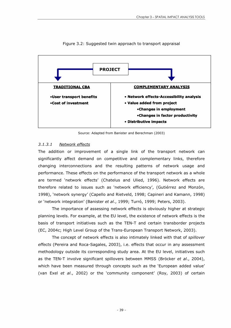
Chapter 3 – SPATIAL IMPACT ANALYSIS TOOLS
- 39 -
Figure 3.2: Suggested twin approach to transport appraisal
TRADITIONAL CBA
•User transport benefits
•Cost of investment
COMPLEMENTARY ANALYSIS
• Network effects-Accessibility analysis
• Value added from project
•Changes in employment
•Changes in factor productivity
• Distributive impacts
PROJECT
TRADITIONAL CBA
•User transport benefits
•Cost of investment
COMPLEMENTARY ANALYSIS
• Network effects-Accessibility analysis
• Value added from project
•Changes in employment
•Changes in factor productivity
• Distributive impacts
PROJECT
Source: Adapted from Banister and Berechman (2003)
3.1.3.1 Network effects
The addition or improvement of a single link of the transport network can
significantly affect demand on competitive and complementary links, therefore
changing interconnections and the resulting patterns of network usage and
performance. These effects on the performance of the transport network as a whole
are termed ‘network effects’ (Chatelus and Ulied, 1996). Network effects are
therefore related to issues such as ‘network efficiency’, (Gutiérrez and Monzón,
1998), ‘network synergy’ (Capello and Rietveld, 1998; Capineri and Kamann, 1998)
or ‘network integration’ (Banister et al., 1999; Turró, 1999; Peters, 2003).
The importance of assessing network effects is obviously higher at strategic
planning levels. For example, at the EU level, the existence of network effects is the
basis of transport initiatives such as the TEN-T and certain transborder projects
(EC, 2004c; High Level Group of the Trans-European Transport Network, 2003).
The concept of network effects is also intimately linked with that of spillover
effects (Pereira and Roca-Sagales, 2003), i.e. effects that occur in any assessment
methodology outside its corresponding study area. At the EU level, initiatives such
as the TEN-T involve significant spillovers between MMSS (Bröcker et al., 2004),
which have been measured through concepts such as the ‘European added value’
(van Exel et al., 2002) or the ‘community component’ (Roy, 2003) of certain

Assessment of Transport Infrastructure Plans: a strategic approach
- 40 -
projects. Clear examples are the national sections of transborder projects2, where
the principle of subsidiarity forces the assessment to be carried out separately
within each country. The exclusion of these effects is argued to make the
profitability of transborder projects, and therefore the public financing they require,
to be systematically under-estimated relatively to purely national projects (Roy,
2003). Moreover, their exclusion also underestimates the benefits related to the
opportunities that transborder projects provide for the promotion of the parallel
development of cross-border regions, which is of crucial importance both for the
EU3 and for particular MMSS (Ollivier-Trigalo, 2001; EC, 1999; EC, 2004b; Turró,
1999).
Hence, it is not surprising to find that so far the analysis of network effects
has been of interest mainly at this EU level (for studies on the subject see van Exel
et al., 2002; Turró, 1999; Pearman et al., 2003; Laird et al., 2005; Bröcker et al.,
2002; Bröcker et al., 2004; Frybourg and Nijkamp, 1998). However, at the national
level, these effects are not usually included in official assessment methodologies
(Bristow and Nellthorp, 2000; Grant-Muller et al., 2001), although they may be of
crucial importance in the assessment of national transport Plans (Condeço and
Gutiérrez, 2006; López et al., 2006a).
3.1.3.2 Value added
This impact category refers mainly to economic development effects, including
those long-term indirect changes in income, output, productivity, and employment,
which are induced by the new opportunities offered by an improvement of the
transport network. The relationship between transport infrastructure improvements
and regional economic development has been and still is a controversial issue for
the research community and the subject of much theoretical and political debates4.
Most authors argue that, under certain market conditions, transport accessibility
improvements can potentially trigger several major positive externalities, which, in
turn, can boost productivity, reduce production costs and promote more efficient
use of resources and, collectively, bring about additional economic development
2 An example of a transborder project is the PBKAL (High-Speed Rail Project Paris-Brussels-Cologne-
Amsterdam-London). The solution for this case was to produce for the EU an European evaluation to
complement the national evaluations of the participating MMSS with a ‘community component’ (Roy,
2003), which provided a rational basis for determining the appropriate level of EU subsidy.
3 Initiatives such as the INTERREG include specifically the objective of cross-border cooperation (EC,
2004b).
4 See Oosterhaven & Knaap, 2003; Banister & Berechman, 2003; Vickerman et al., 1999; Button 1993;
EC 1996a; Banister & Berechman, 2001; Rietveld & Nijkamp, 1993; SACTRA, 1999.

Chapter 3 – SPATIAL IMPACT ANALYSIS TOOLS
- 41 -
benefits. These benefits must be in addition to the primary accessibility
improvement benefits and not merely their market capitalisation. This is the
approach followed in the analytical framework developed by Banister and
Berechman (2003), which highlights the idea that the main output from a transport
investment is network accessibility improvement. Subsequently, two additional
effects may arise:
� Activity spatial redistribution, which, if it ensues, may improve spatial patterns
and economic efficiency,
� Economic development, predicated on the presence of certain market conditions
or ‘allocative externalities’5.
There is consensus in that only in the presence of these positive externalities a
transport project can potentially promote regional economic development (Beuthe,
2002; Banister and Berechman, 2003; SACTRA, 1999). If these externalities are
not present, adding accessibility benefits and potential development benefits would
amount to substantial double-counting of benefits.
Furthermore, there are many other factors influencing the final economic
development effect. One of them is the quality of the transport network, as the
magnitude of the effect seems to depend strongly on the already existing level of
accessibility (Bröcker et al., 2004). It is in regions with low infrastructure qualities
that one expects the highest impacts of infrastructure investments on regional
development, (Button, 1993; Evers et al., 1987; Rietveld and Nijkamp, 1993). In
countries with an already highly developed transport infrastructure further
transport network improvements bring only marginal benefits (Vickerman et al.,
1999). Moreover, the alleged linkage between accessibility improvements and
economic development is being lessened by current trends, as stressed by Banister
and Berechman (2003), namely:
� The declining role of accessibility improvements in the contemporary economies
of cities and regions (Copus et al., 2002),
� the marked change in the relative importance of work related trips and the
increased complexity of commuting patterns6,
5These include a favourable market environment, availability of funds, and supporting legal,
organisational and institutional policies and processes. Under these conditions, the non-compensatory
action of one economic entity can affect the utility level of another, which in turn, can affect the efficient
allocation of resources in the economy (Banister and Berechman, 2003). Traffic congestion is an
example of negative allocative externalities, whereas agglomeration of firms represents positive ones.
6Apparently, the market operates through the relocation of firms and households to achieve the balance
of keeping commuting times within tolerable limits (Banister and Berechman, 2003).

Assessment of Transport Infrastructure Plans: a strategic approach
- 42 -
� the growing importance of information and communications technology in
improved production and distribution processes, compared with transport,
� the concern of reducing travel as a means to achieve the objectives of
sustainable development, which links environmental, economic development
and equity arguments.
Finally, the spatial level of analysis is a key variable influencing the results. If the
analysis is carried out at the highest level of spatial aggregation it may appear that
there is no significant impact on economic growth, while it is possible that spatial
effects do exist but that these relate to distribution effects within regions (Bruinsma
et al., 1997). This issue is discussed in Section 3.1.3.3.
In an attempt to move forward in this research field, there has been in
recent decades an upsurge of different, and sometimes contradictory,
methodological attempts to describe parts of the transport-economy system7. Key
selected models include production functions, (Biehl, 1986; Blum, 1982; ME&P et
al., 2001); accessibility models (Keeble and Owens, 1982; Schürmann et al., 1997;
Bröcker et al., 2002); land-use transport interaction (LUTI) models (van Wee,
2002); and spatial computable general equilibrium (SCGE) models (Salling.K.A. et
al., in press; Laird et al., 2005).
3.1.3.3 Distributive impacts
Improvement of transport infrastructure leads to a reduction of transport costs
which may give rise to substantial redistribution effects among economic groups
and also among regions. (Rietveld and Nijkamp, 1993). This issue is linked with the
trade-off between ‘generative vs. distributive growth’ (Rietveld and Nijkamp,
1993), ‘efficiency vs. equity’ (Bröcker et al., 2004; Feng and Wu, 2003), or
‘competitiveness vs. cohesion’ (EC, 2004a; Gutiérrez, 2004) effects of transport
infrastructure. The three terms distributive, equity and cohesion impacts are used
as almost synonyms in the literature.
Distributive impacts do not refer to the global effect of transport investment,
such as global improvement in accessibility levels, but to its distribution among
regions, frequently addressed as regional equity or cohesion effects, or groups of
individuals, in this case under the social perspective on equity or cohesion
(Schürmann et al., 1997).
7 It is not the purpose of this subsection to describe the theoretical aspects of existing methodological
attempts to describe the complex network of transport-economy linkages (for studies reviewing relevant
methodologies, along with evidence of their fundamental weaknesses and omissions see Nijkamp et al.,
1990; Oosterhaven and Knaap, 2003; Bröcker et al., 2002; Rietveld and Nijkamp, 1993; Aschauer,
1989).

Chapter 3 – SPATIAL IMPACT ANALYSIS TOOLS
- 43 -
Equity motivations have provided the main justification for financing
infrastructure investments in peripheral and/or landlocked regions at the EU level,
as stated in different EU policy documents (EC, 2004a; EC, 2004c; EC, 1999), but
also at national planning levels (see e.g. the case of Germany (BMVBW, 2002), or
Spain (Ministerio de Fomento, 2005). However, their inclusion in appraisal
methodologies is uneven and scarce (Bristow and Nellthorp, 2000; Grant-Muller et
al., 2001), as most CBA studies concentrate on efficiency considerations. However,
it has been suggested that some allowance for distributional impacts should be
incorporated in CBA studies (Button, 1993), or in a MCA framework complementing
the CBA (Beuthe, 2002; ME&P et al., 2001; SACTRA, 1999; Banister and
Berechman, 2003).
The treatment of equity effects is a current challenge for spatial planning
models at strategic levels. Recent research approaches suggest analyzing
distributive impacts in terms of spatial equity impacts8, e.g. via changes in the
spatial distribution of accessibility among regions (Schürmann et al., 1997; Martín
et al., 2004; Bröcker et al., 2004; López, 2005; López et al., in press; INRETS,
2005). Results obtained from these studies show that certain investments may lead
to increasing rather than reducing regional disparities in accessibility, i.e. to a more
polarized distribution of accessibility.
3.2 The potential of accessibility analysis
The use of the accessibility concept has repeatedly been referred to in previous
sections as a useful planning tool which is increasingly included in spatial impact
models. In order to give the reader a more complete understanding of these
references, Section 3.2.1 includes a brief review of the concept of accessibility and
its measurement, while evidence of their potential for spatial impact analysis is
included in Section 3.2.3.
3.2.1 The concept of accessibility
There are many definitions of accessibility and many ways for measuring it. The
concept of accessibility came to the fore in the early 1950s and has a long tradition
in regional science and transport economics, where practical concepts of
accessibility have been widely used for the assessment of the impact of transport
policies on regional economic performance.
8 Distributive issues can also be analysed in terms of social impacts, which requires detailed classification
of the affected population (commonly in terms of low income, disadvantaged groups, etc.). These are
not easy to identify (Banister and Berechman, 2003), especially at strategic planning levels.

Assessment of Transport Infrastructure Plans: a strategic approach
- 44 -
The first basic concept of accessibility related with the ease to reach goods,
services or activities from any given location. One of the first steps forward
appeared when accessibility was also considered in the sense of opportunity or
possibility that people in a certain location have to participate in specified activities.
More recent approaches incorporate social and economic aspects, as they identify
accessibility as the net benefit people of a specific location obtain from the use of
the existing transport and land use system. Still today the concept of accessibility is
still evolving with new approaches that continuously enrich the concept with new
connotations9. This subsection is not aimed at providing an exhaustive list of all
scientific contributions to the concept of accessibility, but a brief review of a
selective list.
Different authors (Gutiérrez, 2004; Martellato et al., 1998; Ney, 2001) have
suggested using the approach used in the accessibility analysis as a tool to review
existing definitions of accessibility. A selection of these approaches is described
bellow.
First, from an infrastructural approach. In this case, accessibility is
exclusively aimed at measuring the performance of the transport system in a
specified area; with accessibility measures such as network density or average
network speed.
Second, from a locational/geographical approach, accessibility is referred to
the degree of separation between locations. This is the approach followed by Morris
et al., (1979), who define accessibility as ‘some measure of spatial separation of
human activities, which denotes the ease with which activities may be reached
using a particular transportation system’.
Third, from a potential of opportunities approach, accessibility is related to
the volume of economic activity that can be reached from any given location,
following the Hansen, (1959) approach to accessibility as ‘the potential of
opportunities for interaction’, or ‘the possibilities of using the opportunities that the
economic, social, cultural and political facilities and institutions provide’ (Domanski,
1979).
Fourth, the utility approach (Koenig, 1980; Ben-Akiva and Lerman, 1979), is
founded in microeconomic welfare theory and it is related to the outcome
individuals obtain from the utilization of the transport system. The latter approach
9 For a review on the theoretical foundations of the concept of accessibility, see Morris et al., 1979; Ney,
2001; Bruinsma and Rietveld, 1998; Reggiani, 1998; Geurs and van Wee, 2004; Geurs and Ritsema van
Eck, 2001.

Chapter 3 – SPATIAL IMPACT ANALYSIS TOOLS
- 45 -
follows a different perspective, as accessibility is not defined as a characteristic of a
location, but that of individuals at a specific location.
The approach used to define the concept of accessibility has motivated aun
upsurge in different formulations for its measurement; i.e. different accessibility
indicators/measures. These are summarized in subsection 3.2.2.
3.2.2 The measurement of accessibility
3.2.2.1 Theoretical background
There is a wide spectrum of existing formulations which attempt to measure the
concept of accessibility. Extensive reviews and existing classifications of
accessibility indicators/measures can be found in Baradaran and Ramjerdi, 2001;
Bruinsma and Rietveld, 1998; Gutiérrez, 2001; García-Palomares, 2000; Handy and
Niemeier, 1997; Reggiani, 1998; Izquierdo and Monzón, 1992; Wegener et al.,
2000; Schürmann et al., 1997; Martellato et al., 1998; David Simmonds
Consultancy et al., 1998; Geurs and Ritsema van Eck, 2001. It is not the purpose
of this subsection to describe the theoretical aspects of accessibility measurement,
but to give an overview of most frequently used indicators. For this purpose, the
approach followed by Schürmann et al., (1997) has been selected from the above
list because of its flexibility to include a wide variety of formulations.
In Schürmann et al. (1997) accessibility indicators are classified according to
their complexity into two broad groups. Simplest accessibility indicators are those
‘infrastructure-based’ (Geurs and Ritsema van Eck, 2001) and only consider the
characteristics of the transport network of the area under consideration. The main
disadvantage of these indicators is that they fail to recognize that many
destinations of interest may lie far away from this area (Wegener et al., 2000;
Geurs and Ritsema van Eck, 2001). There are other types of accessibility indicators
which study the characteristics of the transport network as a whole, but these only
consider the topological properties of network, such as its connectivity. These are
called topological indicators (Mackiewicz and Ratajczak, 1996).
Transport literature is increasingly claiming a ‘paradigm shift’ from the more
traditional infrastructure-based measures towards more complex accessibility
indicators, also called ‘activity-based’ measures (Geurs and Ritsema van Eck,
2001). The common feature of these more complex indicators is that they take into
account not only the characteristics of the transport network but also those of the
land use system which the network is intended to connect. Despite their perceived
complexity, their added value is that they provide complementary information for

Assessment of Transport Infrastructure Plans: a strategic approach
- 46 -
more comprehensive analyses, as they allow testing the efficiency of both land-use
patterns and transport network configurations and their interdependencies.
Schürmann et al., (1997) further classify the most frequently used
formulations of activity-based indicators. Their classification encompasses a great
variety of possible indicators in three generic types, as Equation ( 3.1 ) shows:
( ) ( )ij
j
iji cfWgA ⋅=∑ ( 3.1 )
Following this approach, the accessibility (A) of a given location i is a
construct of two functions, the activity function g, representing the activities or
opportunities (W) to be reached at given locations j, and the travel impedance
function f, representing the ‘effort, time, distance or cost’ (c) needed to reach
them. This is a general form of a gravity model, where the attractors are the
activities or opportunities in areas j, and the distance term is the spatial impedance
cij. The most frequent forms of g and f are represented in Figure 3.310. The different
combinations of both functions result in the corresponding different types of
accessibility indicators.
Figure 3.3: Activity and impedance functions
Source: Schürmann et al. (1997)
Each indicator has specific advantages and drawbacks, although a general
observation is that there seems to be a trade-off between ‘soundness’, i.e.
theoretical and empirical insights, and ‘plainness’, i.e. ease of understanding of
existing formulations (Bertolini et al., 2005; Wegener et al., 2000). Furthermore,
potential improvements in the theoretical foundations of most popular indicators
10 Examples of early formulations of f using are the utilization of a negative potential function (Hansen,
1959) or the negative exponential function conceived by Wilson (1971). Both formulations used distance
as the impedance variable.

Chapter 3 – SPATIAL IMPACT ANALYSIS TOOLS
- 47 -
may imply a loss of their interpretability and therefore they are not being
implemented in most practical accessibility studies (Geurs and Ritsema van Eck,
2001).
Further key improvements of activity-based measures mainly relate to a
dissagregation of individuals according to their socio-economic characteristics
(Bertolini et al., 2005) or the consideration of competition effects11 (Geurs and
Ritsema van Eck, 2001; van Wee et al., 2001). Another weakness comes from the
fact that an increase in destination masses yields a proportional increase in
accessibility, which does not take into account capacity constrains and congestion
risks (Martellato et al., 1998).
Another interesting perspective on accessibility is given by utility-based
measures, which offer an ‘economic’ background for the potential approach. Utility
based measures relate accessibility to the notion of consumer surplus in
microeconomic theory (see Koenig, 1980; Ben-Akiva and Lerman, 1979). This
approach requires accessibility to be measured at the individual level and to model
travel behaviour and the (net) benefits of the users of a transport system. Despite
its ‘methodological significance’ and the many theoretical studies on the subject
(see e.g. Martínez, 1995), these measures are rarely used in empirical applications
(Martellato et al., 1998; Geurs and Ritsema van Eck, 2001).
Finally, another approach is the utilization of space-time prisms (Miller,
1999a). These measures come from space-time geography and take into account
the availability of activities at different times of the day and the times in which
individuals participate in specific activities, given their time-budgets and
restrictions. The applications of these indicators fall beyond the scope of this thesis,
as their large data requirements forces practical applications to be restricted to
relatively small regions and small subsets of the population.
A description of the most frequently used indicators in long-range transport
planning studies, along with a summary of relevant applications are included in
subsections 3.2.2.2 to 3.2.2.4.
3.2.2.2 Travel cost indicators
There is a wide spectrum of formulations under this heading12. Most frequent
formulations measure total or average travel cost to a predefined set of
destinations, as in Lutter et al. (1992) and Schürmann et al. (1997). Other
11 Using inverse balancing factor of singly or double constrained spatial interaction models. A review of
existing approaches can be found in Geurs and Ritsema van Eck, (2001), or Martellato et al.,(1998).
12 Sometimes they are referred to as contour measures with fixed opportunities (Geurs and Ritsema van
Eck, 2001)

Assessment of Transport Infrastructure Plans: a strategic approach
- 48 -
approaches weight destinations according to their size. An example is the location
indicator (Gutiérrez, 2001; Gutiérrez and Urbano, 1996), in which the population of
each destination is used as a weighting factor.
The results of these indicators are inevitable and heavily influenced by the
geographical position, and usually result in core-periphery patterns. This point can
be verified in Figure 3.4, which shows an example of the utilization of a travel cost
indicator for the calculation of European road accessibility13 in 1992.
Figure 3.4: Example of a travel cost indicator. Road accessibility 1992
Source: Gutiérrez and Urbano (1996)
Travel cost indicators are popular because they are expressed in familiar units and
they are easy to interpret, although they lack a behavioural foundation because
they ignore the fact that more distant destinations are visited less frequently
(Schürmann et al., 1997). Furthermore, their values depend heavily on the selected
set of destinations (Wegener et al., 2000).
Other approaches substitute the customary notion of travel cost with that of
network efficiency (Gutiérrez and Monzón, 1998; Monzón et al., 2005). This
substitution highlights the infrastructure effect from that of having a peripheral
geographic location. Figure 3.5 shows an example of an application of a network
13 The indicator is computed as the average road travel time to destinations over 300,000 inhabitants,
expressed in minutes.

Chapter 3 – SPATIAL IMPACT ANALYSIS TOOLS
- 49 -
efficiency indicator in Spain14, for the road mode, before (left) and after (right) the
implementation of the Spanish Transport and Infrastructure Plan (PEIT) (Ministerio
de Fomento, 2005). The indicator is computed as the ratio between real and ‘as the
crow flies’ travel times15 to main population centres. Resulting accessibility contours
show how high-accessibility corridors are concentrated along high capacity
networks, whereas extremely high accessibility values appear in the nodes where
this network converges. Least accessible areas are located outside these corridors,
particularly in mountainous regions. Accessibility contours do not follow core-
periphery patterns: central regions may have low accessibility, whereas peripherally
located regions with efficient connections with the road network may exhibit high
accessibility values.
Figure 3.5: Network efficiency. Road accessibility 2005 (left) and 2020 (right)
Source: López et al. (2006b)
Other examples of travel cost indicators are isochrones, which respond to
the simplest case of a travel cost indicator, where the impedance term is travel
time and only one destination is considered. Other types of indicators frequently
used in planning studies are situational– also called distance (Geurs and Ritsema
van Eck, 2001)- indicators, where the number of destinations are also limited to
14 The map shows predicted accessibility values for the road mode in Spain due to the adoption of the
Infrastructure Master Plan 2005-2020 (PEIT) (Ministerio de Fomento, 2005). This indicator was
previously used in the 2000-2007 Plan (PIT) and the 1993-2007 Master Plan (PDI) (Ministerio de Obras
Publicas y Transportes, 1993).
15 For a detailed description on how these travel times are computed see Gutiérrez and Monzón (1998)
and López et al. (2006).

Assessment of Transport Infrastructure Plans: a strategic approach
- 50 -
one16, but a different destination is selected for each origin area, such as each
inhabitant must be able to reach a bus stop in 5 minutes or should have a bus stop
within 500 metres from their home.
3.2.2.3 Cummulative opportunities indicators
Cummulative opportunities, also called contour (Geurs and Ritsema van Eck, 2001)
indicators, measure the number of opportunities reachable within a given travel
time or distance.
One of the most frequent applications of contour measures at the interurban
scale is the daily17 accessibility indicator. Several accessibility studies have used
this indicator (see Schürmann et al., 1997; Wegener et al., 2000; Gutiérrez, 2001;
Martín et al., 2004; Vickerman et al., 1999). This indicator measures total activity,
usually in terms of population, jobs or GDP, reachable in a given travel time
threshold which is frequently set up between 3 and 5 hours.
Other applications at an international levels use higher time thresholds, such
as 8 hours (Dupuy and Stransky, 1996) or three days (Chatelus and Ulied, 1996).
At the urban scale these values are obviously different, and it is frequent to find
travel time thresholds of 30 minutes (Bertolini et al., 2005).
16 According to the early work of Ingram (1971), these indicators fall into the ‘relative accessibility’
measures, defined as those related to the degree to which two places or points are connected, in
contraposition to ‘integral accessibility’ measures, which take more than one destination into
consideration.
17 The concept of daily accessibility was developed by Törnqvist (1970), from the case of a business
traveler who wishes to travel to a certain city, conduct business there and return home in the evening.

Chapter 3 – SPATIAL IMPACT ANALYSIS TOOLS
- 51 -
Figure 3.6: Daily accessibility indicator. Daily accessibility by rail (1993)
Source: Spiekermann and Wegener (1994)
As an example, Figure 3.6 shows the three-dimensional rail accessibility
surfaces results for a daily accessibility indicator18, computed using raster-based
GIS technology (Schürmann et al., 1997). The map shows how the location of high
accessibility nodes is heavily dependant on the spatial distribution of both
population and railway stations. However, accessibility sharply declines with
distance from these nodes, giving rise to interstitial zones of low accessibility even
in highly accessible central regions, such as the Benelux.
These indicators share with the travel cost indicators their ease of
interpretability, e.g. ‘population reachable in three hours’, and the methodological
drawback of their heavy dependence on the ‘arbitrarily’ selected set of destinations
to be taken into consideration in the analysis. Furthermore, another disadvantage is
that improvements of travel time which do not reduce travel time bellow the
specified threshold do not lead to an improvement in accessibility (Geurs and
Ritsema van Eck, 2001). This drawback is solved if the accessibility measure could
allow a decreasing influence of each destination as travel time increases. This is the
case of potential accessibility measures, which are described in the next section.
18 Results correspond to the rail mode, with population as the mass activity variable and a travel time
threshold of five hours (Wegener et al., 2000).

Assessment of Transport Infrastructure Plans: a strategic approach
- 52 -
3.2.2.4 Potential indicators
Potential indicators are the most popular type of accessibility indicators found in the
literature. The first attempt to use the potential concept to describe accessibility
was developed by Hansen (1959); see Equation ( 3.2 ):
∑=j ij
j
ic
WA ( 3.2 )
Hansen used population and distance as activity (W) and impedance (c)
variables, and introduced a parameter reflecting distance deterrence (beta) equal
to -1. In recent years there has been a widespread application of different
adaptations of this basic Hansen’s formulation, mainly in accessibility studies from
an economic perspective, generally under the assumption that accessibility
deficiencies of certain locations may have influenced their structurally lagging
situation (see e.g. Hansen, 1959; Keeble and Owens, 1982; Bruinsma and Rietveld,
1993; Bruinsma and Rietveld, 1997; Copus, 1999).
In general, potential indicators take into account both the size of
destinations and the travel cost to reach them, under the gravitational based
assumption that the attraction of a destination increases with its size and declines
with travel cost. Most frequent applications follow an exponential negative
impedance function of the form showed in Equation ( 3.3 ):
∑⋅−
⋅=j
c
ji
ijeWAβα
( 3.3 )
where all the terms are already known except for the agglomeration parameter α,
which is usually set up equal to one (Geurs and Ritsema van Eck, 2001; Schürmann
et al., 1997; Gutiérrez, 2001; Martín et al., 2004). The above formula is an
example of the general formula included in Equation ( 3.1 ), with linear and
exponential activity and impedance functions, respectively.
Although potential indicators are widely used in empirical applications, they
have certain limitations (Martellato et al., 1998; Bröcker, 1989; Bruinsma and
Rietveld, 1993), such as their aggregated approach, which implies taking into
account that all individuals in the same zone have the same level of accessibility;
the significant influence that the form of the distance decay function, which should
be tested in an empirical setting, has in the result; the treatment of the ‘self-
potential,’ i.e. the internal component of accessibility, measuring the contribution of
each area to its own accessibility19, or the fact that they are not measured in
familiar units, as it is the case of travel cost measures.
19 The treatment of the self-potential may have considerable influence in the resulting accessibility
values, especially in large agglomerations, as it has important implications for the study of

Chapter 3 – SPATIAL IMPACT ANALYSIS TOOLS
- 53 -
3.2.3 Applications in transport planning
3.2.3.1 Background
It is widely claimed that the potential of accessibility analysis for transport planning
purposes is not fully exploited (Halden, 2003; Geurs and Ritsema van Eck, 2003;
David Simmonds Consultancy et al., 1998; David Simmonds Consultancy et al.,
1998). Indeed, although the concept of accessibility has been widely reported in
geographical studies, it has rarely been used for policy evaluation. It had very little
practical impact on policies (Handy and Niemeier, 1997; Halden, 2002; Ney, 2001),
despite recent interesting attempts to draw formulations related to wider policy
objectives; (see e.g. the work by Bertolini et al., 2005 on the achievement of
‘sustainable accessibility’). Moreover, accessibility analysis has major presentational
advantages by describing the impacts of transport investment in terms that people
can easily understand (Halden, 2000), which is an added value given the increasing
influence of public opinion on these issues.
The lack of practical applications of accessibility analysis in transport
appraisal methodologies is mainly due to concerns about double counting of effects
(Beuthe, 2002; David Simmonds Consultancy et al., 1998; Geurs and Ritsema van
Eck, 2001), the perceived complexity of their formulations and their resulting
difficulty of interpretation (Geurs and Ritsema van Eck, 2003). Each of the
formulations of accessibility described in Section 3.2.2 is particularly suited to
address a certain transport planning problem. However, the selection of the
appropriate indicator for a particular case is a complex task. Moreover, there is
evidence that the formulation chosen, mainly the choice of the distance decay
function, has a strong influence in the results obtained (Baradaran and Ramjerdi,
2001). In general there is no single best ‘ideal’ indicator, but it is argued that the
analysis is enriched if a set of indicators is computed and their results analyzed in a
complementary way (see e.g. Gutiérrez, 2001; Martín et al., 2004; Schürmann et
al., 1997).
An analysis of the use of accessibility indicators for transport planning
purposes is given in the following sections. First, the use of accessibility
improvements as a policy goal by itself is analyzed in section 3.2.3.2.
Subsequently, and following the SD approach, the following subsections include
agglomeration economies (Bruinsma and Rietveld, 1993; Bruinsma and Rietveld, 1997). It requires the
computation of an ‘internal travel time.’ Although there is a wide variety of approaches that handle the
self-potential problem, it is still a controversial issue (for studies dealing with this issue see, for example
Bruinsma and Rietveld, 1997; Bruinsma and Rietveld, 1993; Frost and Spence, 1995; Bröcker, 1989).

Assessment of Transport Infrastructure Plans: a strategic approach
- 54 -
evidence of the utility of accessibility indicators for the assessment of wider policy
impacts from the economic (subsection 3.2.3.3) and social (subsection 3.2.3.4)
sustainability dimensions. The use of accessibility analysis from an environmental
perspective is less frequent and therefore has not been addressed here (for one of
the few existing approaches see e.g. Sánchez and Zamorano, 2006).
3.2.3.2 Accessibility improvement as a policy goal
The need for plans to evaluate their accessibility impacts is emphasized in many
national planning policy guidance (see e.g. DETR, 2000; Scottish Executive, 2000;
Ministerio de Fomento, 2005). ‘Accessibility improvement’ as a policy goal by itself
has been widely included among the key objectives of transport infrastructure plans
and programmes. For example, in Spain the impact of transport infrastructure
improvements on accessibility was included in the evaluation of the Plan Director de
Infraestructuras 1993-2007 (PDI) (Gutiérrez and Monzón, 1998) and the recently
launched Plan Estratégico de Infraestructuras y Transporte (PEIT) (López et al.,
2006b). Another example is the UK case, in which ‘accessibility’ is one of the five
assessment criteria of the ‘New approach to appraisal’ (NATA) (DETR, 1998). At the
European level, accessibility impacts of TEN-T have been the subject of many
studies (see e.g. Gutiérrez and Urbano, 1996; Schürmann et al., 2004; Chatelus
and Ulied, 1996; Lutter et al., 1992).
3.2.3.3 Economic perspective
In most economic studies public infrastructure is measured according to the
amount of public capital stock. This implies some limitations, mainly that the quality
of public infrastructure in each region is only measured in terms of its infrastructure
stock and that spatial spillover effects are usually ignored. These problems may be
remedied using some measure of the economic accessibility of each region –the
economic potential model-, instead of the stock of infrastructure (Rietveld and
Nijkamp, 1993; Bruinsma and Rietveld, 1997; Oosterhaven and Knaap, 2003; de
Orellana-Pizarro, 1994). The economic potential measure gives an aggregate
measure of the market area of each region, resulting in a deceptively reduction in
potential accessibility as we move away from the centre (Vickerman et al., 1999).
Obviously, the potential accessibility formulation gives a more realistic
approximation of the increase in economically useful opportunities available to a
certain region that will result from a transport network improvement. Moreover,
using accessibility instead of transport stock makes it possible to show that not only
the region where the actual investment takes place will profit from improved
accessibility, but also to take into account network and spillover effects, since they

Chapter 3 – SPATIAL IMPACT ANALYSIS TOOLS
- 55 -
are capable of assessing the effects of a single link on a transport network
(Gutiérrez and Monzón, 1998; Halden, 2003; Geurs and Ritsema van Eck, 2001).
Accessibility analysis can be used to assess network effects of improved links in a
certain country on neighbouring countries (López et al., 2006a). Furthermore, it
can be applied to any transboundary project, i.e. referring to any administrative
boundaries, where competency issues are also of concerns for DMs (for recent
applications at the national level see e.g. Condeço and Gutiérrez, 2006; López et
al., 2006a).
Moreover, it is even argued that the wide establishment of comprehensive
composite accessibility methods may provide a more accurate assessment of the
economic value of transport improvements than the one derived from travel
demand models, which are frequently less than fully comprehensive at national
planning levels (Halden, 2003; David Simmonds Consultancy et al., 1998). Most
scientific contributions have attempted to provide evidence of the relationship
between accessibility and economic development (for a review of relevant
contributions see Rietveld and Nijkamp, 1993). However, the few satisfactory
empirical investigations of the role of accessibility as a means to promote regional
economic activities provide uncertain (and controversial) results (Beuthe, 2002).
Some examples of quite modest effects are impact of the motorway system on the
regional distribution of employment in 28 regions in the UK (Botham, 1983), the
analysis of the effect of the M62 in the UK (Dodgson, 1974), or the London M25
orbital (Linneker and Spence, 1996), the extension of the USA highway system
(Kau, 1976), a new railway line in the Amsterdam-Hamburg corridor (Evers et al.,
1987), the fixed link across the Great Belt in Denmark (Illeris and Jakobsen, 1991),
the relationship between accessibility and the attractiveness of Dutch cities for
situating economic activities (Bruinsma and Rietveld, 1997), or the investigation
carried out by Ozbay et al. (2003) on the impacts of accessibility changes on the
level of economic development of 18 counties in the New Jersey/New York region.
Moreover, accessibility indicators can be used as a tool for the economic
evaluation of transport planning initiatives, as reviewed by Geurs and Ritsema van
Eck (2001). This research work includes applications of accessibility indicators in
three approaches, following Bruinsma et al. (1997): a CBA approach, a production
function approach, and an employment approach. They are briefly described below.
3.2.3.3.1 Accessibility and CBA
In a social cost benefit analysis (CBA) several authors have shown that utility-based
accessibility measures can be used to estimate consumer surplus (Neuburger,
1971; Williams, 1976; Handy and Niemeier, 1997). Essentially, the idea is that a

Assessment of Transport Infrastructure Plans: a strategic approach
- 56 -
measure of consumers surplus (expressed in utility) can be derived by taking the
natural logarithm of a potential accessibility measure with a negative exponential
distance decay function.
The use of utility-based measures in the measurement of consumer surplus
has advantages compared to standard CBA, as reviewed in Geurs and Ritsema van
Eck (2001). One of them is that it enables the measurement of both the benefits of
an improved transport system and changes in the land-use system. Another
strength is its potential to analyse equity aspects (i.e. it can be used to analyse
which individuals or groups of individuals living in certain locations benefit from
changes in accessibility), since the benefits of changes in accessibility can be
located to regions.
However, the theoretically correct use of utility-based measures for
measuring consumer surplus requires a transport model which properly forecasts
the combined land-use transport equilibrium, including land-use and transport
feedbacks (van Wee, 2002; Geurs and Ritsema van Eck, 2003).
3.2.3.3.2 Accessibility and the production function approach
In literature, most empirical studies using the production function approach have
estimated the effects of total public capital on economic growth. Much less the
impacts of transport infrastructure development. Very few of the impacts of
accessibility changes on productivity and economic growth (see the review on this
topic carried out by Geurs and Ritsema van Eck, 2001).
One of the few examples of a study on the relationship between
infrastructure, accessibility and economic development was carried out in the
context of the SASI project (Wegener et al., 2000) and its follow-up project EUNET
(ME&P et al., 2001) and IASON (Tavasszy et al., 2004), where an ‘extended’ SASI
model was used. The SASI recursive simulation model estimates the socio-
economic impacts of transport infrastructure investments and transport system
improvements, based on empirically derived production functions with activity-
based accessibility indicators as a variable, as outlined in Figure 3.7.

Chapter 3 – SPATIAL IMPACT ANALYSIS TOOLS
- 57 -
Figure 3.7: Outline of the SASI model
Source: Schürmann et al. (1997)
As an example of an application of the SASI model, Figure 3.8. shows changes in
GDP per capita as a result of the (at that time) planned TEN-T priority projects for
the year 2020.

Assessment of Transport Infrastructure Plans: a strategic approach
- 58 -
Figure 3.8: Changes in GDP per capita as a result of the planned TEN priority projects
Source: Tavasszy et al. (2004)
Of particular interest are the Spanish studies carried out in the 1980s
(Izquierdo et al.,1980; SENDA 3, 1986) on the economic implications of
accessibility improvements, and the study by de Orellana-Pizarro (1994), who
developed a production function approach to assess regional economic development
effects of the Spanish Master Plan 1993-2007 based on changes in accessibility
values.
3.2.3.3.3 Accessibility and employment
Although employment effects are often considered important in the analysis of
infrastructure projects, especially in regions with chronic underemployment,
employment effects of a typical transport project are generally considered to be
temporary and distributive (Geurs and Ritsema van Eck, 2001).
There are few studies on employment effects based on the use of
accessibility indicators. An example is the study by Bruinsma et al. (1997) who
investigated the relationship between highway construction, potential accessibility
to employment and regional employment growth in the Netherlands, found no
simple mono-casual relationships. Another approach is the one followed by Ozbay
et al. (2006), based on the approach suggested by Berechman and Paaswell

Chapter 3 – SPATIAL IMPACT ANALYSIS TOOLS
- 59 -
(2001). They used an accessibility function, transportation data’ weighted travel
time, as an input to develop an employment function in terms of several socio-
economic variables. These functions were tested in the New York/New Jersey
metropolitan area and the Bronx County in New York, respectively. The main
results showed that accessibility parameters are statistically significant for the
employment function, but that changes in accessibility have rather modest effects
on net employment growth.
3.2.3.4 Social perspective
Despite the debate on the effects of accessibility on economic development,
detailed in Section 3.1.3.2, regional development studies have traditionally been
based on the assumption that the uneven spread of development is a function of
spatial inequalities in accessibility (EC, 1996b). Accessibility is therefore seen as an
added value of a location and an important factor of quality of life (Schürmann et
al., 1997), and in a sense a proxy for measuring welfare, if we accept that the
welfare of individuals is related with the ease which they can access essential
services (Hay, 1995).
Early examples of the use of accessibility to assess cohesion impacts date
back to late 1970s, such as the study by Domanski (1979), who relates the
increase of accessibility to spatial concentration. This author uses accessibility as a
measure to represent spatial equity, essentially by applying the potential formula to
a hypothetical spatial system. Under this general approach, accessibility is often
considered in regional planning as a means to economic activity and cohesion,
rather than a desirable good by itself (Vickerman et al., 1999).
Therefore, changes in the distribution of accessibility values among regions
may be used as a proxy for measuring regional cohesion; whereas differences in
accessibility among individuals or groups of individuals may play the same role in
assessing of social cohesion impacts. The regional cohesion approach is more
generally used at wider geographical levels. The social perspective is more widely
used at a local level, given the large amount of information that the disaggregation
of the population requires according to their socio-economic characteristics.
3.2.3.4.1 Accessibility and regional cohesion
Spatial distribution of accessibility is one of the variables included in the ‘check-list’
of the periodical Cohesion Reports of the European Union (EC, 2004a), among
which are included macroeconomic indicators such as GDP per capita, employment
levels or R&D investments. The rationale behind the inclusion of accessibility in this
list is that the ‘equality of access to services of general economic interest’ is

Assessment of Transport Infrastructure Plans: a strategic approach
- 60 -
considered a key condition for territorial cohesion (Peters, 2003). Special interest is
placed in regions with geographical handicaps characterized by problems of
accessibility and integration with the rest of the EU. Infrastructure investment is
thus considered a key factor in order to provide a fair distribution of accessibility to
all its regions and to reduce existing disparities in accessibility between them
(Schürmann et al., 1997).
However, transport investment and increased regional cohesion do not
follow a causal relationship. Some scientists even argue, that better transport links
between strong and competitive centres and economically weak peripheries may
increase polarisation instead of cohesion (Hey et al., 2002). It can be concluded
that at the regional level redistribution will take place, often as additional
advantage to the already accessible parts of the country (Banister and Berechman,
2003).
Accessibility differences can therefore be used to assess equity impacts. It is
claimed that horizontal and vertical equity should be considered to minimize the
intraregional difference in accessibility for the main cities in the same region and to
minimize that interregional difference among regions, respectively (Feng and Wu,
2003). Existing attempts to use accessibility for the computation and visualization
of regional cohesion impacts can be found mainly at the European level. An
example is the study by Bruinsma and Rietveld (1993), who used a population
potential indicator to analyse if disparities of accessibility values in 42 major
European agglomerations increased with the implementation of planned
infrastructure investments. They found that inequalities in accessibility are least
pronounced in the road network, than in the rail network. A similar study using four
different accessibility indicators was carried out by Martín et al. (2004), in this case
to assess cohesion effects of a HSR line. Changes in the spatial distribution of
accessibility were also used to measure regional cohesion impacts at the EU level in
the SASI (Schürmann et al., 1997), ESPON (Bröcker et al., 2004), and IASON
(Tavasszy et al., 2004) projects. This type of analysis becomes less frequent as the
geographical scale is narrowed (for existing approaches at the national and regional
levels see e.g. López, 2005; Condeço and Gutiérrez, 2006).
The above studies show that many factors influence the final impact on
regional cohesion, such as the geographical scale of the analysis (Martín et al.,
2004), given that there may be positive equity impacts at the regional level but not
at a national level, or the existing development level of the network considered
(Martín et al., 2004; López, 2005), as in under-developed regions, efficiency is

Chapter 3 – SPATIAL IMPACT ANALYSIS TOOLS
- 61 -
usually the main concern and it is difficult for DMs to justify investments on the
basis of equity considerations.
The assessment of regional cohesion effects following this accessibility
approach can be included in strategic assessment methodologies, although existing
attempts are mostly found only in research applications (see ME&P et al., 2001;
INRETS, 2005; Bröcker et al., 2004; López and Monzón, 2006).
3.2.3.4.2 Accessibility and social cohesion
Accessibility indicators are increasingly used in social cohesion studies, mainly at
the local level with a focus on public transport. These studies are related to the
assessment of social exclusion issues of transport policies (Lucas, 2006). For this
purpose, accessibility is usually dissagregated by population groups, what allows
focusing in the situation of disadvantaged sectors of the population, such as aging
population or low income workers. Recent examples are: Lucas, 2006; Preston and
Rajé, in press; Lau and Chiu, 2003 and Alsnih and Hensher, 2003. Other
applications focus in the situation of population of rural areas and low density zones
(Nutley, 2003), equity mapping (Talen and Anselin, 1996; Talen, 1998),
distribution of job accessibility (Cervero et al., 1995; Geurs and Ritsema van Eck,
2003), or social changes (Halden, 2002; Bröcker et al., 2004).
3.3 Spatial impact and GIS
3.3.1 GIS background
Geographical Information Systems (GIS) can be defined20 as ‘a suite of methods for
capturing, storing, analysing and communicating geo-referenced information’
(Miller, 1999b). The history of GIS dates back to the 1950s21, when early
applications of GIS emerged for land use management and environmental impact
assessment activities supported by government agencies in Canada and the United
Sates. The emergence of computer-assisted cartography in the 1970s constituted a
crucial step in the development of GIS. Then, during the 1980s and 1990s there
were several important technical and organizational developments that greatly
assisted the current wide application and appreciation of GIS.
Today, although GIS technology is still evolving, it has already reached a
certain maturity, with existing applications in a wide spectrum of fields such as
20 See Burrough and McDonnell (1998) for a review of existing definitions of GIS.
21 See Foresman, 1998; Burrough and McDonnell, 1998 for a detailed chronology of GIS evolution.

Assessment of Transport Infrastructure Plans: a strategic approach
- 62 -
agriculture, tourism, navigation, or archaeology. Recent applications show a
tendency towards the integration of GIS and Global Positioning Systems (GPS) (see
e.g. Taylor et al., 2000).
GIS database management capabilities and the usefulness of advanced
operations and functions allow performing integrated analysis of spatial and
attribute data22, especially useful in spatial impact analysis (Nijkamp et al., 1990).
Figure 3.9: Superposition of data layers in GIS for a transport study.
Source: Taylor et al. (2000)
As an example, Figure 3.9 shows a diagram illustrating the use of GIS as a
database integrator for a transport study area. The GIS is able to integrate a
mixture of spatial, numerical, and perhaps textual datasets, and display them by
superposition of separate map layers, such as topographical and land use, transport
network infrastructure, socioeconomic and demographic, traffic flow, and pollution
22 A comprehensive review of GIS operations can be found in Burrough and McDonnell (1998) and
DeMers (1997).

Chapter 3 – SPATIAL IMPACT ANALYSIS TOOLS
- 63 -
and environmental impacts. The Figure also indicates the areas of modelling and
analysis involving the use of different subsets layers, such as travel demand
modelling or impact analysis. There is a wide list of literature on the integration of
GIS and spatial models (Wegener, 2001; Nijkamp et al., 1990; Fotheringham and
Wegener, 2000). Spatial analysis is currently benefiting from the new geo-
computational tools that are emerging from geographic information science (GISci),
a new interdisciplinary field that focuses on the theory and techniques behind GIS
and related technologies (Goodchild, 1992). However, the tools offered by current
GIS do not usually include the analytical and modelling capabilities needed for
spatial modelling (Wegener, 2001). Indeed, the potential synergies between GIS
and spatial models are not fully exploited (Miller, 1999b).
Furthermore, recent development of computer programs have enabled GIS
platforms to provide user friendly interfaces so that analysts and planners can
execute model runs and analyze model results without the need for GIS
technicians, which is considered one of current’s primary benefits (Miller and Storm,
1996). All the above capabilities make GIS specially suited at providing support in
situations where decision making is required (Nijkamp et al., 1990; Malczewski,
1999; Arampatzis et al., 2004; Miller, 1999b). This is the case with transport
planning processes.
3.3.2 Applications of GIS in transport planning
3.3.2.1 GIS and transport planning processes
GIS capabilities make them specially suited for each of the three stages of transport
planning process described in Chapter 2. First, GIS can have a relevant role to play
in the structuring stage. The capabilities of GIS are useful for data organisation,
ease of data entry, data processing and visualisation, and for the detection of
deficiencies/problems and subsequently set the corresponding planning objectives.
This may constitute a critical issue. Indeed, it is argued that the way the planning
problem is represented has a major importance for DMs, as seemingly minor
variations in the way the problem is represented can lead to different
recommendations (Guitouni and Martel, 1998). The above advantages are making
both private and public agencies increasingly rely on GIS as indispensable tools for
planning and decision making.
Second, the use of GIS in the evaluation stage is also widespread (Nijkamp
et al., 1990; Malczewski, 1999; Gómez and Bosque, 2004; Arampatzis et al.,
2004). The capability of GIS to provide, at any time, appropriate information

Assessment of Transport Infrastructure Plans: a strategic approach
- 64 -
regarding trade-offs and efficiency of proposed solutions has created an increase in
their popularity in recent years (Miller, 1999b). Key approaches use GIS to support
accessibility calculations (Liu and Zhu, 2004; Zhu and Liu, 2004; Gutiérrez and
Monzón, 1998; Miller and Wu, 2000), environmental assessments (Antunes et al.,
2001; Colorni et al., 1999; Li et al., 1999; Brown and Affum, 2002), network
demand models (Miller, 1999b; Miller and Storm, 1996) , traffic congestion studies
(Taylor et al., 2000), alignment optimization models (Jha and Schonfeld, 2004;
Sadek et al., 1999) or regional (Bröcker et al., 2002) and urban spatial planning
models (Wegener, 2001).
Third, in the decision-making stage a GIS ‘serves to contribute at solving,
organizing and rationalizing complex choice and decision problems’ (Nijkamp et al.,
1990). The development of GIS has exerted a deep on-going impact on modern
decision analysis, enabling the design of interactive user-oriented multiple criteria
decision models (MCDM) (Malczewski, 1999; Sadek et al., 1999; Klungboonkrong
and Taylor, 1999) or Decision Support Systems (DSS) (Arampatzis et al., 2004;
Colorni et al., 1999; Jha, 2003) especially useful in transport decision-making
processes, where the stakeholders can be a large and diverse group (Miller and
Storm, 1996). In this sense, the ‘communicative’ abilities of GIS due to their
capabilities to create high standard visual images could be more fully exploited in
order to stimulate discussion and evaluation of different project designs in new and
more informative ways (Grant-Muller et al., 2001).
However, despite the above mentioned advances, a more integrated work of
spatial analysis, transportation and GIS research communities could have a
substantial positive impact on the theory and practice of transportation analysis and
planning (Miller, 1999b; Wegener, 2001). This constitutes a current challenge for
the research community.
3.3.2.2 GIS and accessibility analysis
Finally, this subsection describes the use of GIS to compute most of the
accessibility indicators described in section 3.2. Given the spatial nature of
accessibility, GIS have become a useful tool for accessibility analysis, which
provides capabilities for data collection, data management and manipulation,
spatial analysis, network analysis, and cartographical presentation of accessibility
measures.
A description of the steps required for the use of GIS to compute
accessibility indicators can be found in Zhu and Liu (2004), who developed an
integrated GIS approach to accessibility analysis, which is illustrated in Figure 3.10.
This approach consists of six major processes or elements: problem definition and

Chapter 3 – SPATIAL IMPACT ANALYSIS TOOLS
- 65 -
data collection, query and data retrieval, measure selection and specification, travel
impedance measurement, calculation of accessibility measures and visualization of
accessibility values.
Figure 3.10: An integrated GIS approach to accessibility analysis.
Source: Zhu and Liu (2004)

Assessment of Transport Infrastructure Plans: a strategic approach
- 66 -
3.4 Conclusions
At the Plan level, additional assessments are necessary to address wider policy
impacts such as network effects or distributive impacts, usually not covered by
traditional appraisal methodologies such as CBA (SACTRA, 1999; Beuthe, 2002).
Most of these impacts have a spatial component and therefore modern spatial
impact models are especially suited for these tasks.
Accessibility indicators could potentially be used as a criterion for project and
policy appraisal (David Simmonds Consultancy et al., 1998; Halden, 2003; Ney,
2001) which could complement existing methodologies. Further research is needed
to take advantage of this unexploited potential and develop formulations combining
a theoretically sound foundation and a relative ease of interpretation for DMs and
the public opinion.
Furthermore, special care is needed for the inclusion of accessibility analysis
in appraisal frameworks, as the addition of accessibility impacts to the CBA results
would generally have a double-counting of effects. However, accessibility indicators
can be introduced in MCA frameworks, although it is essential to define with
precision what the accessibility analysis is meant to represent or to which policy
objective it corresponds in order to attribute a sensible weight in the MCA. For
example, if weights varying inversely with the level of economic development are
used, accessibility results may be useful to compute the projects impact on social
cohesion under the assumption that improved accessibility induces economic
development (ME&P et al., 2001; BMVBW, 2002). A possible alternative is to
compute inequality indices of the spatial distribution of accessibility among regions,
in order to measure regional cohesion impacts (Schürmann et al., 1997; López and
Monzón, 2006). Another possibility is to use accessibility results in a MCA to
measure political issues, such as international network integration, but in this case
it should be made explicit that the objective is political and not economic (Beuthe,
2002).
Finally, a current challenge for the research community is to take full
advantage of recent developments of GIS to develop a more integrated work of
spatial analysts, transportation planners and GIS capabilities. This integration could
result in significant synergies and have a substantial positive impact on the theory
and practice of transportation analysis and planning (Miller, 1999b; Wegener,
2001).

Chapter 4 – METHODOLOGY FOR THE ASSESSMENT OF TRANSPORT INFRASTRUCTURE PLANS
- 67 -
4. METHODOLOGY FOR THE ASSESSMENT OF
TRANSPORT INFRASTRUCTURE PLANS
Chapter 2 concluded that national transport Infrastructure Plans assessment
methodologies need to adapt to a new planning framework. Chapter 3 reviewed
recent developments in assessment tools and techniques. In the light of these
findings, this Chapter describes a methodology for the assessment of Transport
Infrastructure Plans. The structure of this methodology is outlined in Section 4.1.
The structure of the proposed procedure is built on the definition of the assessment
framework, described in subsection 4.2, and assessment criteria, defined in
subsection 4.3. Performance indicators linking model outputs and assessment
criteria are defined in subsection 4.4. Finally, subsection 4.5 outlines the
foundations of a MCA framework for the integration of assessment results.
4.1 Structure of the methodology
The proposed methodology is suggested as a tool to complement traditional
assessment methodologies at the Plan level. The proposed approach suggests a
procedure to assess those strategic aspects which are usually not included in official
methodologies, despite the fact that they are very important for the achievement of
transport policy goals.
The methodology is flexible in the sense that the final integration of their
results with that of the traditional methodologies, such as a CBA, has intentionally
been left for the consideration of DMs. This responds to the fact that, at the Plan
level, as discussed in Section 2.4., the technical appraisal plays an important role
but the final decision is usually influenced by a set of external constraints, mainly of
a political nature.
Figure 4.1 shows the structure of the proposed methodology, which is fully
implemented in a GIS. The process is built from two starting points, following a
twin approach (Brown et al., 2001):
� A ‘top-down’ approach: The identification of strategic policy objectives
constitutes the main guidelines to the definition of assessment criteria,

Assessment of Transport Infrastructure Plans: a strategic approach
- 68 -
� A ‘bottom-up’ approach: The definition of the different alternatives to be
assessed is necessary for the models to forecast the impacts of the transport
projects under consideration.
Figure 4.1: Structure of the methodology
DEFINITION OF ALTERNATIVES
POLICY OBJECTIVES
GIS
PERFORMANCE INDICATORS
ASSESSMENT CRITERIA
ANALYSIS OF RESULTS
ACCESSIBILITY/TRANSPORT MODELS
INTEGRATION (MADM)
INPUT DATABASE
SENSITIVITY ANALYSIS
DEFINITION OF ALTERNATIVESDEFINITION OF ALTERNATIVES
POLICY OBJECTIVES
POLICY OBJECTIVES
GIS
PERFORMANCE INDICATORS
ASSESSMENT CRITERIA
ANALYSIS OF RESULTS
ANALYSIS OF RESULTS
ACCESSIBILITY/TRANSPORT MODELS
ACCESSIBILITY/TRANSPORT MODELS
INTEGRATION (MADM)
INPUT DATABASE
INPUT DATABASE
SENSITIVITY ANALYSIS
The accessibility and the transport models provide the main inputs for
impact assessment. Subsequently, in order to measure the performance of each
alternative in each assessment criteria, a set of performance indicators1, linking
model outputs with each assessment criteria is defined.
The added value of the methodology is mainly included in the design of the
assessment criteria and the corresponding set of performance indicators. The main
singularity of the proposed approach is that the accessibility model is the driving
engine of the assessment methodology. Indeed, most performance indicators
include accessibility indicators in their formulation. The rationale behind their
inclusion is that changes in the values and the spatial distribution of accessibility
indicators can be used as proxy variables for the assessment of strategic impacts,
taking advantage of their unexploited potential in transport assessment
methodologies (see Section 3.2.3.).
The results obtained in each performance indicator need to be subsequently
integrated in order to obtain a single score for each alternative. This is dealt with in
the application of a multiatribute decision making (MADM) method. The process is
subsequently complemented with a sensitivity/robustness analysis of the results to
1 Also referred to as measures of performance (Brown et al., 2001).

Chapter 4 – METHODOLOGY FOR THE ASSESSMENT OF TRANSPORT INFRASTRUCTURE PLANS
- 69 -
key parameters and external factors of the evaluation process. Finally, conclusions
and recommendations on the best performing alternative are provided to the DMs2.
4.2 Definition of the assessment framework
4.2.1 Assessment time horizon
The assessment of alternatives is carried out at the planning time horizon (tp),
previously defined in the Plan. The performance of each alternative is compared
against the ‘do-nothing’ alternative (A0), defined as that with the same network as
the one existing in the base year (t0). This comparison is outlined in Figure 4.2.
External inputs for the accessibility and transport models, such as population
growth, are defined identical between alternatives, in order to isolate the effects
stemming from the infrastructure changes from those derived from the
development of external variables.
Figure 4.2: Comparison of alternatives
NETWORK BASE YEAR A0
NETWORK ALTERNATIVE A1
NETWORK ALTERNATIVE AN
NETWORK BASE YEAR A0
BASE YEAR t0PLANNING TIME
HORIZON tp
NETWORK BASE YEAR A0NETWORK BASE YEAR A0
NETWORK ALTERNATIVE A1NETWORK ALTERNATIVE A1
NETWORK ALTERNATIVE ANNETWORK ALTERNATIVE AN
NETWORK BASE YEAR A0NETWORK BASE YEAR A0
BASE YEAR t0PLANNING TIME
HORIZON tp
This scheme requires making a prognosis concerning the future development
of these external variables. The assessment procedure therefore relies on the
accuracy of this prognosis which, given the long-term planning horizons of most
Plans, introduces high levels of uncertainty in the results. The methodology handles
2 On the basis of these conclusions, the possibility for the inclusion of feedback loops (see e.g. Nijkamp
et al., 1990) in the procedure is represented by the dotted lines in Figure 4.1.

Assessment of Transport Infrastructure Plans: a strategic approach
- 70 -
this issue in the sensitivity analysis step, with the definition of assessment
scenarios.
4.2.2 Delimitation of the study area
The analysis done in Section 3.1.3.1 shows that the effects of transport Plans
extend beyond the administrative boundaries of the region or nation concerned,
generating spillover effects. In order to assess these effects, the limits of the study
area should be widened over these administrative boundaries. However, this
extension of the study area faces some political and technical drawbacks, mostly if
the additional territories belong to other countries. On the one hand, DMs are
usually exclusively concerned with the effects produced inside the frontiers of the
territories in their competency, even if the Plan is supported with ‘external’ funds,
as it is the case of national Plans supported by European funds. On the other hand,
the inclusion of information from different countries makes the assessment
procedure more data demanding and complex, as these data usually need to be
harmonised with national data sources.
This issue is dealt with in the methodology with the adoption of a compromise
solution for the delimitation of the study area. The proposed approach consists in
widening the study area to include those regions in which spillover effects may
appear. As will be detailed in this Chapter, the specific treatment of these ‘external’
regions in the assessment procedure is different than that of the territory for which
the Plan has been originally designed.
4.3 Definition of assessment criteria
Assessment criteria have been selected based on the review of recently developed
research studies, national official assessment methodologies and most relevant EU
policy documents carried out in Section 2.2.3. These studies mostly agree that at
the Plan level current traditional appraisal procedures, mainly based on CBA
approaches, should be complemented with the assessment of certain wider
strategic objectives/criteria and be consistent with the triangular SD approach.
Hence, this methodology suggests complementing traditional assessment
methodologies with the assessment of strategic assessment criteria. The structure
of these criteria and corresponding subcriteria is included in Table 4.1. This
structure responds to the SD approach: i.e efficiency is related to the economic,
cohesion to the social and environmental sustainability to the environmental SD
dimensions. The policy relevance of each subcriterion and their detailed description
is included in subsequent sections.

Chapter 4 – METHODOLOGY FOR THE ASSESSMENT OF TRANSPORT INFRASTRUCTURE PLANS
- 71 -
Table 4.1: Assessment criteria
CRITERIA SUB-CRITERIA
Network efficiency Efficiency
Cross-border integration
Regional cohesion Cohesion
Social cohesion
Global warming Environmental sustainability
Habitat fragmentation
4.3.1 Efficiency
The term efficiency embraces different concepts, such as competitiveness, network
efficiency, regional development, economic development or growth. The efficiency
of transport links between major economic activity centres is considered as one of
the factors determining competitiveness (EC, 2004a). These activity centres may be
located inside or outside the national boundaries; therefore the improvement of
cross-border links is frequently included as a policy goal for improved
competitiveness, particularly in peripheral countries, such as Spain (Ministerio de
Fomento, 2005). Moreover, cross-border cooperation is intended to develop cross-
border economic and social centres through joint strategies for sustainable
territorial development (EC, 2004b).
The methodology takes into account this issue by splitting the efficiency
criterion into two subcriteria, namely (national) network efficiency and cross-border
integration. This is done in order to split efficiency benefits accruing to the study
area under consideration from those that occur in neighbouring cross-border
regions, as they respond to different policy goals and therefore the DM will probably
attach a different preference strength to each one of them.
4.3.2 Cohesion
Among the wide variety of existing approaches included under the cohesion heading
(see Section 3.1.3.3.), the methodology focuses on two issues which are of
increasing interest among transport planners at strategic levels. These issues are
regional and social cohesion.
Regional cohesion effects are assessed with the analysis of whether the Plan
increases or reduces existing disparities in the spatial distribution of accessibility
among regions. This increase or reduction can be interpreted as a negative or
positive regional cohesion effect, respectively. The concern derived from the

Assessment of Transport Infrastructure Plans: a strategic approach
- 72 -
tendency of certain transport infrastructure extensions to induce polarising effects
are therefore also addressed.
The contribution of the Plan to the social cohesion objective is handled in the
methodology with the exploration of a possible contribution of accessibility
improvements to regional development in lagging regions. This contribution would
result in a more balanced distribution of socio-economic conditions among social
groups: those living in lagging regions and those that do not. This balancing effect
is usually termed as an enhanced social cohesion.
The social cohesion criterion is aimed at measuring to what extent
accessibility benefits are accruing to structurally backward regions, whilst the
regional cohesion criterion analyses effects stemming from changes in the spatial
distribution of accessibility; i.e. the objective is to investigate whether the
accessibility improvements derived from the Plan increase or reduce existing
disparities in accessibility among regions. The focus of the regional cohesion
criterion is therefore exclusively limited to the changes in the regions’ relative
positions in terms of accessibility, independently from their economic development
level.
4.3.3 Environmental sustainability
Climate change, loss of biodiversity due to habitat fragmentation, effects on human
health (e.g. local emissions) and well-being due to accidents, air quality and noise
are the most important environmental concerns related to transport activity3 (EEA,
2003). Only the first two -climate change and habitat fragmentation- have been
selected from this list because of their strategic nature; the rest are frequently
addressed at the project level (see Section 3.1.2.2.).
First, the climate change phenomenon is directly linked to energy
consumption and directly related to green house gas (GHG) emissions. These are
strategic environmental aspects of great interest due to both the need to comply
with international environmental commitments and the urgency to reduce energy
consumption, which has a greater economic component.
Second, the assessment of habitat fragmentation due to transport
infrastructure has been included since it is recognised globally as one of the biggest
threats to the conservation of ecological biodiversity, which should be ideally
addressed at strategic levels. The assessment of habitat fragmentation i.e. the
‘dynamic process of splitting of habitats into smaller and more isolated areas, called
3 Transport and Environment Reporting Mechanism. Periodical reports are published by the European
Environment Agency (EEA) and are available at http://reports.eea.eu.int/.

Chapter 4 – METHODOLOGY FOR THE ASSESSMENT OF TRANSPORT INFRASTRUCTURE PLANS
- 73 -
patches’ (Burel and Baudry, 2002) remains a contentious issue, where there is a
lack of commonly accepted procedures for its assessment4.
The selection of fragmentation indices5 is an important aspect of assessment
procedures (Riitters et al., 2004). The perimeter and the area of each patch are
probably its most important and useful variables from an ecological point of view
and therefore are usually included in the formulation of fragmentation indices. On
the one hand, the shape of the patches is directly linked with the ‘border effect’:
the higher the perimeter, the higher the threat from external factors. On the other
hand, the presence and wealth of many species is intimately linked with the area of
the patch (Robbins et al., 1989).
4.4 Definition of performance indicators
Figure 4.3 describes the interdependence between the outputs of the models and
performance indicators.
Figure 4.3: Performance indicators’ inputs
INFRASTRUCTURE NETWORKSOCIO-ECONOMIC VARIABLES
ACCESSIBILITY CALCULATIONS TRAFFIC FLOWS
TRAVEL IMPEDANCES
LANDSCAPE QUALITYINPUT
GW
Global warming
HF
Habitatfragmentation
NE
Networkefficiency
CB
Cross-borderintegration
RC
Regional cohesion
SC
Social cohesion
MODELLING
PERFORMANCE INDICATORS
INFRASTRUCTURE NETWORKSOCIO-ECONOMIC VARIABLES
ACCESSIBILITY CALCULATIONS TRAFFIC FLOWS
TRAVEL IMPEDANCES
LANDSCAPE QUALITYINPUT
GW
Global warming
HF
Habitatfragmentation
NE
Networkefficiency
CB
Cross-borderintegration
RC
Regional cohesion
SC
Social cohesion
MODELLING
PERFORMANCE INDICATORS
4 For a review on impacts of transport infrastructure on habitat fragmentation, see Riitters et al., (2004)
and Burel and Baudry (2002).
5 Usually based on raster land-cover information derived from satellite imagery. The value of the index
obtained is particularly sensitive to the spatial and theme distribution of the input map. National
ecological assessment procedures typically handle this issue computing a small number of indices and
analysing their results in a complementary way.

Assessment of Transport Infrastructure Plans: a strategic approach
- 74 -
Depending on their input data requirements, performance indicators can be
classified as follows:
� Based on accessibility results: network efficiency, cross-border integration,
regional cohesion and social cohesion.
� Independent from modeling results: habitat fragmentation.
� Based on transport flows in the whole system: global warming.
Table 4.2 gives an overview of the assessment criteria and their corresponding
performance indicators. Their detailed formulation is explained below.
Table 4.2: Assessment criteria and performance indicators
CRITERIA PERFORMANCE INDICATOR
EFFICIENCY
Network efficiency Change of network efficiency in national
territories
Cross-border integration Change of network efficiency in cross-border
regions
COHESION
Regional cohesion Change in synthetic inequality index of
accessibility indicators
Social cohesion Standardised increase in potential
accessibility of isolated and/or lagging
regions
ENVIRONMENTAL SUSTAINABILITY
Global warming Change in GHG emissions
Habitat fragmentation Change in habitat fragmentation index
4.4.1 Efficiency
4.4.1.1 Network efficiency
The main input variable for this performance indicator is the network efficiency
accessibility indicator (E) (Gutiérrez and Monzón, 1998; Gutiérrez, 2001), using
Equation ( 4.1):
∑∑
⋅
=j
j
j
j
ij
ij
iP
PII
I
E ( 4.1 )

Chapter 4 – METHODOLOGY FOR THE ASSESSMENT OF TRANSPORT INFRASTRUCTURE PLANS
- 75 -
This indicator is used to calculate, for each i-j pair, a weighted mean of
ratios between travel time using the network (Iij) and an ‘ideal’6 travel time (IIij).
The population of each destination (Pj) has been selected as the weighting factor.
The set of origins i is restricted to those belonging to the national territory, whereas
the set of potential destinations j includes national as well as cross-border economic
activity centres.
For each alternative s, the performance indicator – NEs - calculates the
percentage change, compared with the do-nothing alternative A0, of a population-
weighted aggregated value of the network efficiency accessibility indicator,
according to the formulation detailed in Equation ( 4.2 ):
100
0
0 ⋅
−
=
∑∑
∑∑
∑∑
r
i
i
i
i
sr
i
i
i
i
i
i
i
i
i
s
P
PE
P
PE
P
PE
NE ( 4.2 )
4.4.1.2 Cross-border integration
This performance indicator is also measured using the network efficiency
accessibility indicator as the main input variable. The main difference lies in the
definition of the spatial coverage, as the set of origins only includes those nodes (r’)
located in cross-border regions of neighbouring countries, whilst the set of
destinations is the same as that used for the assessment of national network
efficiency impacts. Hence, benefits accruing outside the national boundaries
(spillover effects) are accounted for.
Equation ( 4.3 ) includes the formulation of the performance indicator – CBs -
, where all the terms have already been defined:
100
0
0
*
*
*
*
*
*
*
*
*
*
*
*
*
*
*
⋅
−
=
∑∑
∑∑
∑∑
rr
r
rr
srr
r
rr
rr
r
rr
s
P
PE
P
PE
P
PE
CB ( 4.3 )
6 Measured as travel time as the crow flies, with 120 km/h speed for road mode and 220 km/h for rail
mode.

Assessment of Transport Infrastructure Plans: a strategic approach
- 76 -
4.4.2 Cohesion
4.4.2.1 Regional cohesion
This performance indicator is based on the analysis of disparities in the spatial
distribution of accessibility. The rationale behind this analysis is that accessibility
can be considered as an ‘added value’ of locations, in a way related to their level of
welfare. Hence, disparities in accessibility among regions can be used as a proxy
variable for the measurement of territorial cohesion effects.
The choice of the accessibility indicator depends on the purpose of the study,
as analyzed in Section 3.2.2. In this context, where cohesion is analysed under a
welfare perspective, the most suited accessibility indicator is the potential indicator.
Among existing formulations (see Section 3.2.2.4.), the one selected has proved its
validity in similar studies (Martín et al., 2004). It is described in Equation ( 4.4 ):
∑=j ij
j
rI
PPP ( 4.4 )
There is a wide variety of statistical indices capable of characterising the
level of dispersion of any given variable; they are referred to as inequality
measures/indices7. The variable under analysis here is potential accessibility, hence
each inequality index is computed combining the accessibility values of individual
regions (PPr) into one single measure of their spatial concentration. The population
of each individual region (Pr) has been selected as the weighting variable.
The choice of the inequality index may have a strong influence on the results
(Bröcker et al., 2004; Schürmann et al., 1997). Therefore, four of the most
commonly used inequality indices are computed and their results analysed in a
complementary way.
The four inequality indices are compared with their corresponding values in
the ‘do-nothing’ alternative. Then, the regional cohesion performance indicator
(RCs) is computed as the mean value of the resulting relative change in the four
inequality indices, as expressed in Equation ( 4.5 ). In every case, a lower value of
the index represents a more equal distribution, and vice versa. A brief description
of each of the indices is included below8.
−+
−+
−+
−⋅=
0
0
0
0
0
0
0
0
4
1
Th
ThTh
At
AtAt
Gi
GiGi
CoV
CoVCoVRC ssss
s ( 4.5 )
7 Inequality measures are commonly used in the economic literature for the analysis of income
distribution. For a comprehensive review on inequality measurement, see Cowell (1995).
8 For an extensive description of these and other inequality indices, see Cowell (1995).

Chapter 4 – METHODOLOGY FOR THE ASSESSMENT OF TRANSPORT INFRASTRUCTURE PLANS
- 77 -
The first one is the coefficient of variation (CoV): it is computed as the ratio
between the standard deviation and the mean (µ).
µ
deviation standard=CoV ( 4.6 )
The second one is the GINI coefficient (Gi). It is a summary statistic of the
Lorenz curve, a cumulative frequency curve that compares the distribution of a
specific variable with the uniform distribution that represents equality. The Gini
coefficient ranges from a minimum value of zero, when all individuals are equal, to
a theoretical maximum of one in an infinite population in which every individual
except one has a size of zero. It corresponds to twice the area between the Lorenz
curve and the diagonal (perfect equality).
Third, the Atkinson index (At) is computed using Equation ( 4.7):
εε
µε
−−
⋅−= ∑
1
11
1)(i
i
i
xpAt if 1≠ε
⋅−= ∑
i
i
i
xpAt
µε logexp1)( if 1=ε
( 4.7 )
Where pi is the percentage of population and xi is the proportion of total
accessibility enjoyed by the ith group, respectively, and ε is the so-called inequality
aversion parameter. The parameter ε reflects the strength of society's preference
for equality, and can take values ranging from zero to infinity. When ε > 0, there is
a social preference for equality (or an aversion to inequality). As ε rises, society
attaches more weight to income transfers at the lower end of the distribution and
less weight to transfers at the top. Typically used values of ε include 0.5 and 2.
Finally, the Theil index (Th) is part of a larger family of measures referred to
as the General Entropy class. Its formulation is as follows:
∑
⋅=
i i
ix
pThµ
log ( 4.8 )
4.4.2.2 Social cohesion
This performance indicator calculates a weighted sum of regional accessibility
changes. Each region’s weighting factor (Φr) depends on its level of structural
backwardness and of that of accessibility deficiencies in the do-nothing situation, as
Table 4.3 shows. Weighting factors vary from zero-point minimum to a four-point

Assessment of Transport Infrastructure Plans: a strategic approach
- 78 -
maximum in case of coincidence of accessibility deficits with high levels of economic
backwardness, according to the following matrix:
Table 4.3: Weighting factor matrix for the cohesion criterion
Accessibility deficiencies
Structural backwardness
category
None Not very
significant
Significant Very
significant
Non-lagging regions 0 1 1 2
Potentially lagging regions 1 1 2 3
Lagging regions 1 2 3 4
Source: Adapted from BMVBW (2002) and Bröcker et al. (2004)
The typology of lagging regions is based on a single or a combination of
socio-economic indicators9, usually unemployment rates and GDP per capita levels,
depending on data availability. All regions are ranked and classified according to the
standards defined in Table 4.4.
Table 4.4: Structural backwardness categories
CATEGORY Structural backwardness Cells per type
Substandard 0 Non-lagging regions Best 50%
Substandard 1 Potentially lagging 50% to 30%
Substandard 2 Lagging Worst 30%
On the other hand, the classification in accessibility levels is split into four
categories. The definition of the substandard of accessibility categories is included
in Table 4.5.
Table 4.5: Accessibility analysis categories
CATEGORY Accessibility deficiencies Cells per type
Substandard 0 None Best 50%
Substandard 1 Not very significant 50% to 25%
Substandard 2 Significant 25 to 10%
Substandard 3 Very significant Worst 10%
For the selection of accessibility indicators to be used in the model, three
possibly conflicting objectives are considered to be relevant (Bröcker et al., 2004):
first, the accessibility indicators should contribute as much as possible to explaining
9 For example, a possible combination is the one followed by Bröcker et al. (2004): the unemployment
rate weighted by 60 percent, GDP per head weighted by 40 percent.

Chapter 4 – METHODOLOGY FOR THE ASSESSMENT OF TRANSPORT INFRASTRUCTURE PLANS
- 79 -
regional economic development. Second, the accessibility indicators should be
meaningful in themselves as indicators of regional quality of life. Third, the
accessibility indicators should be consistent with theories and empirical knowledge
about human spatial perception and behaviour. In the light of these objectives the
formulation of the population potential accessibility indicator (PPr), included in
Equation ( 4.4 ), was adopted.
The social cohesion performance indicator –SCs- is calculated as the ratio
between the weighted (by the corresponding population and the social cohesion
weighting factor) accessibility increase and the population-weighted accessibility
value of the do-nothing alternative, expressed in percentage terms.
100
)(
0
0
⋅⋅
−⋅⋅
=
∑
∑
∑
∑
r
r
r
r
r
r
r
r
s
rr
r
r
s
P
PPP
P
PPPPP
SC
φ
( 4.9 )
Hence, above average accessibility improvements in lagging regions are
given higher weights in the final value, therefore measuring the relative
contribution of each alternative to social cohesion. The interpretation of this
indicator is as follows: the higher values, the more the concentration of higher
accessibility improvements for those individuals of structurally lagging and/or
inaccessible regions, i.e. the higher contribution to the social cohesion objective.
4.4.3 Environmental sustainability
4.4.3.1 Gobal warming
The selected performance indicator for the global warming criterion is total
greenhouse gas emissions (GHG), measured in equivalent tons of CO2. CO2
emissions are included as indicators for climate change issues in different
environmental indicator lists (see Banister et al., 2000b; EEA, 2003; OECD, 1998).
Annual CO2 emissions are computed and summed up to calculate total tons of CO2
emitted in each alternative, using the vehicle-kilometres-travelled generated by the
transport model per mode and the information on the national vehicle fleet (drives,
car categories and emission standards).

Assessment of Transport Infrastructure Plans: a strategic approach
- 80 -
4.4.3.2 Habitat fragmentation
The availability and level of disaggregation of environmental information on
landscape quality is uneven among MMSS. Therefore, for the definition of the
patches the methodology proposes to use existing EU-level databases containing
harmonised land-cover information and to complete them with additional country-
specific information, in case this is available10. In particular, the definition of
patches is suggested to be based on existing landscape information on habitats
included in the Habitats Directive 92/43/EEC11. All the available land cover
information is subsequently aggregated to obtain a final GIS vectorial map with the
spatial classification of habitat types.
The selected fragmentation index is the Perimeter/Area RAtio (PARA). It is a
widely used ‘spatial configuration index’ 12 to calculate (see Equation ( 4.6 )) the
ratio between the perimeter (Pe) and the area (Ar) of each patch (i).
i
i
iAr
PePARA = ( 4.10 )
The GIS capabilities allow analysing how the perimeters and areas of all
patches comprising each habitat are affected when they are crossed by the road
and rail infrastructure network extensions included in the Plan. Transport
infrastructure is considered as a total barrier, i.e. a new infrastructure is considered
to divide every patch it crosses into smaller patches.
Figure 4.4. represents an example of the fragmentation produced in a
specific patch (drawn in the left Figure), when it is crossed by a highway and hence
fragmented into 5 smaller patches (drawn in the right Figure).
10 In this sense, CORINE (Land cover dataset firstly developed in the 1990s as part of the European
Commission programme to COoRdinate INformation on the Environment ) datasets can, to a certain
extent, be interpreted with regard to its potential land use and hence recognise areas being mainly
natural or semi-natural, receiving low human impact. However, some anomalies may appear when
assessing landscape fragmentation based only on CORINE information (EC, 2000).
11 Council Directive 92/43/ECC of 21 May 1992 on the conservation of natural habitats and of wild fauna
and flora, O. J. L 206, 22.07.92.
12 It is beyond the scope of this thesis to include a review on the concept and measurement of habitat
fragmentation. The reader is referred to Jaeger (2000), Riitters et al. (2004) and McGarigal and Marks
(1995) for selected literature reviews on the topic.

Chapter 4 – METHODOLOGY FOR THE ASSESSMENT OF TRANSPORT INFRASTRUCTURE PLANS
- 81 -
Figure 4.4. Scheme of the calculation of the PARA index
The corresponding values of the PARA index in the original situation (Figure 4.4
left) and the new situation (Figure 4.4 right) have been included in Table 4.6.
Table 4.6: Example of the computation of PARA values
PATCH Area (m2) Perimeter (m) PARA % increase in PARAOriginal patch 1,697,521.84 9,877.70 0.0058 -Patch # 1 920,980.58 6,169.39 0.0067 15.12Patch # 2 406,845.16 2,980.34 0.0073 125.89Patch # 3 66,975.51 1,083.20 0.0162 277.94Patch # 4 58,430.32 1,097.32 0.0188 322.74Patch # 5 63,480.74 1,258.97 0.0198 340.83
This index is measured at the patch level and subsequently aggregated
using the area of each patch as the weighting variable.
∑∑∈
∈
⋅=
hi
hi
i
ii
hAr
ArPARAPARA
( 4.11 )
For each alternative, the value of the PARA index is computed as the
weighted mean of PARA indices among habitats, using each habitat area as the
weighting variable:
∑∑
⋅=
h
h
h
hh
Ar
ArPARAPARA
( 4.12 )

Assessment of Transport Infrastructure Plans: a strategic approach
- 82 -
Finally, for each alternative, the habitat fragmentation performance indicator
is computed as the percentage change in the PARA index, if compared to that of the
do-nothing alternative, as Equation ( 4.13 ) shows:
1000
0⋅
−=
PARA
PARAPARAHF
s
s ( 4.13 )
4.5 Integration
4.5.1 Outline of the proposed approach
The objective is to obtain a ranking of the n alternatives on the basis of the results
of the performance indicators (X) in each of the m (6 in this case) criteria. The
aggregation of performance indicators to obtain an overall score for each
alternative constitutes a multiattribute decision making (MADM) problem.
The value/utility function approach has been selected from the vast list of
available MADM methods13. The standard assumptions underlying this method
involve preferential independence (i.e. the relative preferences of attributes are not
altered by changes in other attributes) and utility independence (i.e. the utility
function over a single attribute does not depend on the other attributes).
The utility function method is based on multiattribute utility theory (Keeny
and Raiffa, 1976). The term utility function is restricted to a probabilistic criterion
or decision under uncertainty, when the DMs’ attitudes toward risk are an important
determinant of the final results. This approach involves the estimation of the value
(utility) function f and the scaling constant (weight) wj for each attribute14. As
Equation ( 4.14) shows, by multiplying the utilities by the weights, the trade-offs
among the attributes utilities are taken into account in the multiattribute utility
function:
∑ ⋅=j
sjjs uwU ( 4.14 )
Where Us is the overall utility of the s-th alternative, wj is a normalized
weight or scaling constant for attribute j, and usj is the utility of the sth alternative
with respect to the jth attribute, measured by means of the utility function. The
procedures to determine criteria’s weights and utility functions are explained in
Sections 4.5.2 and 4.5.3, respectively. The procedure is outlined in Figure 4.5.
13 A comprehensive review of MADM methods can be found in Malczewski, 1999; Keeny and Raiffa,
1976; Goodwin and Wright, 1991; Nijkamp et al., 1990.
14 Criterion is a generic term including the concepts of attribute and objective, whereas an attribute is
used to measure performance in relation to an objective (Malczewski, 1999).

Chapter 4 – METHODOLOGY FOR THE ASSESSMENT OF TRANSPORT INFRASTRUCTURE PLANS
- 83 -
Figure 4.5: The integration procedure
ALTERNATIVE 1 ... j ... m
1
...
s Xs1 Xsj XSm
...
n
CRITERIA
ALTERNATIVE 1 ... j ... m
1
...
s us1 usj usn
...
n
CRITERIA
U1
...
Us
...
Un
PERFORMANCE MATRIX
PARTIAL UTILITY MATRIX
GLOBAL UTILITY VECTOR
)( sjsj Xfu =
∑ ⋅=j
sjjs uwU
ALTERNATIVE 1 ... j ... m
1
...
s Xs1 Xsj XSm
...
n
CRITERIA
ALTERNATIVE 1 ... j ... m
1
...
s us1 usj usn
...
n
CRITERIA
U1
...
Us
...
Un
PERFORMANCE MATRIX
PARTIAL UTILITY MATRIX
GLOBAL UTILITY VECTOR
)( sjsj Xfu =
∑ ⋅=j
sjjs uwU
4.5.2 Weight estimation
The suggested method to derive the base weight profile is the REMBRANDT
procedure (Lootsma, 1992), based on the Analytical Hierarchy Process (AHP),
originally developed by Saaty (1990). REMBRANDT is one of the best known
attempts to retain the strengths of AHP while avoiding some of its objections
(Tsamboulas et al., 1998).
The procedure requires conducting a questionnaire in which the respondent
is asked to express his/her strength of preferences between pairs of criteria on a
qualitative scale, which corresponds to numerical values in a -8/+8 interval. These
values form the elements of the pairwise comparison matrix of jxj elements, which
are subsequently transformed15 into the estimated criteria weights.
15 The procedure uses a direct rating system which is based on a logarithmic scale to replace the 1 - 9
scale of AHP and exchanges the eigenvector-based synthesis approach for one which is based on use of
the geometric mean.

Assessment of Transport Infrastructure Plans: a strategic approach
- 84 -
The required information was obtained from a survey conducted in different
transportation-related events16. The questionnaire and the average resulting weight
profile obtained are included in Appendix A.
The procedure described above is aimed at computing a base weight profile.
These weights will be subsequently used as a starting point to define a set of
weight profiles. The sensitivity of the results to changes in criteria weights will be
assessed in the sensitivity analysis step of the methodology, as it is detailed in
Section 4.6.
4.5.3 Utility functions
The selected procedure to derive each criterion’s utility function is the indifference
technique (Keeny and Raiffa, 1976). It requires the DM to assess an outcome that
will make him/her indifferent between this outcome and a gambling of two other
values that already have a utility value.
A pointwise approximation of the utility function can be obtained by asking
the DM a series of questions such as: for attribute j, what certain outcome xj would
be equally desirable as realizing the highest outcome with a probability p and the
lowest outcome with a probability of 1-p? This can be expressed in utility terms
using the extreme xj+ and xj- as:
( ) ( )( ) ( )−+ ⋅−+⋅== jjjjjj xupxupxu )1(? ( 4.15 )
where uj(xj) is the utility function associated with the jth attribute, and uj(xj+)=1 and
uj(xj-)=0 are the utilities of the best and the worst outcomes for the jth attribute,
respectively. The extreme values of the outcomes, xj+ and xj- are therefore
necessary to construct the functions. To construct the utility curve, a set of
questions need to be asked to the DM until enough discrete points have been
assessed to give an accurate picture. Usually three points is enough (Martínez-
Falero and González-Alonso, 1995).
4.6 Sensitivity analysis
Sensitivity analysis is a collection of methods used for evaluating how sensitive the
outputs are to small changes in the input values (Malczewski, 1999). The most
important elements to consider in sensitivity analysis are criterion weights and
criterion (attribute) values.
16 VI Transportation Engineering Congress (CIT 2004), Doctorate Transport Policy Course (academic year
2003/2004) of the Civil Engineering School of the Polytechnic University of Madrid. The sample contains
a total of 38 questionnaires.

Chapter 4 – METHODOLOGY FOR THE ASSESSMENT OF TRANSPORT INFRASTRUCTURE PLANS
- 85 -
4.6.1 Weight sensitivity
Sensitivity to attribute weights is perhaps more important than to attribute values,
because they are the essence of value judgments (Malczewski, 1999). The
suggested approach consists in systematically carrying out sensitivity tests varying
the weights attached to each criterion, in order to detect the values that provoke a
shift in the ranking of alternatives. The comparison of the ranking of alternatives
obtained using each weight profile makes it possible to analyse the robustness of
the results to changes in the preference strength attached to each criterion.
4.6.2 Attribute value sensitivity
The other sensitivity concern is sensitivity due to errors in estimating the attribute
values. The values obtained depend on many factors beyond the control of the DM.
These uncontrollable factors are referred to as states of nature or states of
environment (Malczewski, 1999). The states of nature, such as the state of the
economy (e.g. recession, inflation) reflect the degree of uncertainty about decision
outcomes. For each alternative there is a set of possible outcomes, depending on
the corresponding state of nature.
One popular procedure to deal with different states of nature is the design of
scenarios. A scenario represents a plausible assumption on the future development
of external factors: i.e. it represents a particular state of nature. Therefore,
scenario construction techniques (see Rehfeld, 1998; Banister et al., 2000a; Hey et
al., 2002) allow isolating the impacts caused by transport infrastructure
improvements from the ones stemming from the, unknown, future development of
external variables to the assessment procedure.
The assessment procedure defines nxm scenarios (S) as a combination of n
network alternatives (A) and m assumptions on the development of these external
variables (E), as Table 4.7. shows.
The reference scenario (S00) combines a business-as-usual (BAU) prognosis
of external variables, and a ‘do-nothing’ network alternative, i.e. that with the
network of the base year. The comparison of scenarios of the same line, when
compared to the ones of the reference scenario, allow for the isolation of the effects
of a new infrastructure. In contrast, the comparison of scenarios of the same row
gives insight into the effects of changes in the development of external variables.

Assessment of Transport Infrastructure Plans: a strategic approach
- 86 -
Table 4.7: Matrix for scenario building
NETWORK ALTERNATIVES
A0
(Do-nothing) A1 … … An
E0
(BAU)
S00
(Reference
scenario)
S01 S0n
E1 S10
…
…
EXTERNAL
VARIABLES
Em Sm0
Finally, the resulting ranking of alternatives under different scenarios allows
for the assessment of the robustness of the results to external factors of the
methodology.

Chapter 5 – CASE STUDY DESCRIPTION
- 87 -
5. CASE STUDY DESCRIPTION
The case study will deal with the assessment of the extension of the Spanish High
Capacity Road (HCR) and High-Speed Rail (HSR) networks as included in the
Spanish Transport and Infrastructure Strategic Plan 2005-2020 (PEIT) (Ministerio
de Fomento, 2005). The PEIT objectives have a strategic nature and they include
the enhancement of the transport system’s efficiency and its general sustainability,
the contribution to social and territorial cohesion and the promotion of economic
development and competitiveness. This strategic nature makes the PEIT especially
appropriate for the application of the proposed methodology. This Chapter first
includes an Introduction, and Section 5.1, with some specific aspects of the
application of the methodology. The case study is subsequently briefly
characterized in Section 5.2. Finally, the assessment framework is described in
Section 5.3.
5.1 Introduction
The methodology described in Chapter 4 is aimed at providing an integrated
assessment framework for a hypothetical situation in which the planner is
confronted with the problem of selecting one from a set of alternatives for the
extension of a national transport infrastructure network.
The case study described in this Chapter provides a first approximation to
the full application of the methodology, which allows testing its validity. However,
the full application of the methodology is beyond the scope of this thesis, as it
would require a great amount of data processing work as well as the existence of
already developed modeling tools, which is not the case for Spain. One of these
modeling tools is a national transport demand model (see Figure 4.3.).
Unfortunately, Spain has not yet developed its own transport demand model,
although its development is currently included in the Government’s research
agenda. This problem has been solved with the utilization of average travel time
elasticities in order to roughly estimate traffic growth derived from the capacity
extension. The calculation of GHG emissions faces a similar problem, as it requires
the existence of an inventory of vehicle fleet composition and related emission

Assessment of Transport Infrastructure Plans: a strategic approach
- 88 -
factors. This issue has been solved using TREMOVE (Transport & Mobility Leuven
and K.U.Leuven, 2006), a pre-existing model at a EU scale.
Another issue is the selection of one out of a set of network alternatives. The
case study does not handle this issue, as it assesses the effects of the already
approved alternative: the one included in the PEIT. However, the methodology has
included a MCA framework in order to allow for the possibility to select one among
a set of alternatives. The design of a fictitious set of alternatives would have
constituted an interesting theoretical research exercise but it would have implied
again a great amount of modeling work.
In summary, although a full application of the methodology is hindered by the
above limitations, the validity of the fundamental scientific added value of the
suggested approach is considered to be sufficiently tested with its application to the
case study, which has made it possible to test the robustness of the method and its
explanatory potential of strategic effects.
5.2 Case study characterization
Spain constitutes an interesting case study in an EU context. Due to its status of
cohesion country it has received substantial support from European Funds for its
infrastructure development in the last two decades. This was particularly the case
for transport, in which Spain received a third of the total investment in improving
the transport network in Objective 1 regions over the periods 1994-99 (CEC, 2001)
and 2000-2006 (EC, 2004), contributing in an average of some 20%-30% of the
Ministry of Public Works and Transport infrastructure expenditure (Ministerio de
Fomento, 2005). These investments were mainly dedicated to the extension of the
Spanish HCR and HSR networks.
The result has been that Spain has reduced its disparities in network
endowment with the rest of the EU significantly. This fact, along with the
progressive convergence of Spanish GDP per capita values has meant that this
financial support will be substantially reduced in the near future.
This subsection provides the reader with contextual information on the case
study so that the assessment results included in Chapter 6 can be correctly
interpreted and analyzed. For this purpose, it includes a review of the current
situation of the transport infrastructure networks (subsection 5.2.1) and the socio-
economic system (subsection 5.2.2). Subsequently, the main challenges of the
Spanish transport system are described in subsection 5.2.3.

Chapter 5 – CASE STUDY DESCRIPTION
- 89 -
5.2.1 The surface transport infrastructure networks
5.2.1.1 Road network
Figure 5.1 represents the Spanish1 structural road network, which comprises a total
of 24,797 km divided into national, regional and local roads. The High Capacity
Road (HCR) network has a marked radial nature and comprises 10,200 kilometers
of highways, dual carriageways and toll motorways.
Figure 5.1. Spanish road network (2005)
Source: Ministerio de Fomento (2005)
The improvements of the Spanish road network were historically done
through the development of a hierarchical radial road structure, which gave rise to
a higher polarization of the spatial system. This has motivated the corresponding
economies of scale and contributed towards economic development and European
integration objectives (Ministerio de Fomento, 2005). However, although this radial
structure has a number of advantages in terms of network efficiency, its spatial
equity effects are not desirable (EC, 1999). The main challenges for the road
network are its transformation from its radial structure into a grid mesh and a
reduction of the surface of the areas with accessibility deficiencies.
1 Canary Islands, Ceuta, Melilla and the Balearic Islands are not included in this description of the
transport system. In what follows, the term “Spanish” will be referred to as the national territory
included in the Iberian Peninsula.

Assessment of Transport Infrastructure Plans: a strategic approach
- 90 -
5.2.1.2 Rail network
The Spanish rail network is basically constituted by nearly 14,000 km of
conventional rail network (Iberian track gauge) and nearly 1,100 km of high-speed
rail network (UIC track gauge). The HSR network is therefore in an underdeveloped
stage compared to that of the HCR. A huge investment effort is currently been
made to transfrom the conventional rail network into a HSR network, in order to
improve rail accessibility and to harmonize it with the rest of the European network.
Similarly to the HCR network, the rail network also presents a marked radial
nature, as Figure 5.2 shows.
Figure 5.2. Spanish rail network (2005)
Source: Ministerio de Fomento (2005)
5.2.2 The socio-economic system
5.2.2.1 Administrative divisions
The classification of the Spanish territory into administrative boundaries, its number
and its correspondence with the EU’s NUTS2 nomenclature have been summarized
in Table 5.1 and has been represented in Figure 5.3.
2 Nomenclature of Territorial Units for Statistics

Chapter 5 – CASE STUDY DESCRIPTION
- 91 -
Table 5.1: Spanish administrative divisions and their NUTS correspondence
Administrative unit NUTS level # of divisions
Group of Autonomous Regions NUTS-13 7
Autonomous region NUTS-2 17
Province NUTS-3 50
Municipality NUTS-5 8,109
Figure 5.3: Spanish NUTS divisions
5.2.2.2 Spatial distribution of population
Spain suffers from a rather polarized spatial distribution of population. The two
main urban agglomerations are Madrid and Barcelona, which together account for
nearly 26% of total population4. These two cities and coastal areas concentrate the
higher population densities (see Figure 5.4), whereas less populated areas are
located in inner and/or rural areas, which furthermore suffer from progressive
population falls.
3 The areas belonging to NUTS-1 level are not governed or controlled by a specific national entity. This
division was only made with statistical aims. 4 Data obtained from the INE (National Statistical Institute) database.

Assessment of Transport Infrastructure Plans: a strategic approach
- 92 -
Figure 5.4: Population density
Source: Ministerio de Vivienda (2005)
The Spanish system of cities has a hierachical structure, constituted of
(Ministerio de Fomento, 2004a):
� International metropolitan areas: Madrid and Barcelona, which represent the
two major attraction poles of the system.
� National metropolitan areas, defined as those with population between 500,000
and 1,500,000 inhabitants. Their scarcity and highly polarized spatial
distribution hinders a balanced development and favors the appearance of weak
areas throughout the country.
� Sub-regional capitals: this level includes province capitals and urban
agglomerations over 50,000 inhabitants. In this level there is a higher spatial
balance. In general, coastal areas are sufficiently structured around these sub-
regional capitals, whereas inner areas suffer from higher deficiencies with large
areas with unstructured urban systems.
� The rest of capitals and urban areas: they include the rest of province capitals
and cities or urban agglomerations under 50,000 inhabitants.
Figure 5.5 represents the system of cities of the study area.

Chapter 5 – CASE STUDY DESCRIPTION
- 93 -
Figure 5.5: Study area system of cities
Source: National Statistics Institute (INE)
During the last few decades there has been a trend towards the
consolidation of this polarizing process of the spatial distribution of the population.
In this context, the current main challenges for the Spanish spatial system are to
reverse the processes of concentration, agglomeration and conurbation of
settlements; densification of coastal areas; preservation of North-South
imbalances, and the upsurge of large underpopulated or low density areas
(Ministerio de Vivienda, 2005).
5.2.2.3 Spatial distribution of economic activity
The Spanish economy has grown at higher rates than EU average in the last two
decades, which has facilitated its convergence with average GDP per capita UE
levels, from 87% of EU25 in 1996 to 97% in 2003. Northeast and Madrid NUTS-2
regions are those concentrating higher GDP per capita levels, above EU25 average,
whereas South, Centre and Northwestern regions suffer from below average GDP
levels, as Figure 5.6 shows.

Assessment of Transport Infrastructure Plans: a strategic approach
- 94 -
Figure 5.6: Growth in GDP per head in Spain, Spanish NUTS-2 regions and EU15 in terms of EU25 average (PPS5) 1995-2003
60
70
80
90
100
110
120
130
140
150
1995 1996 1997 1998 1999 2000 2001 2002 2003
year
GDP per head in PPS (Spain=100)
EU25 EU15 Spain Noroeste Noreste
C. Madrid Centro Este Sur
Source: EUROSTAT
These marked disparities in regional income per capita levels within Spanish
regions do not show a balancing trend. This can be observed in Figure 5.7 : Spanish
higher and lower income regions have kept their relative position in terms of the
national average for the 1995-2003 period, whereas EU25 and EU15 values have
converged with that of Spain. From a cohesion perspective, this unequal regional
development is unacceptable6.
5 Purchasing Power Standard. 6 Donaghy (2003) analyzes differences in Spanish regional economies and how these differences might
be taken into account in designing policies to reduce regional inequality.

Chapter 5 – CASE STUDY DESCRIPTION
- 95 -
Figure 5.7: Trends in GDP per head in Spanish NUTS-2 regions, EU15 and EU25 in terms of Spain’ average, 1995-2003
60
70
80
90
100
110
120
130
140
150
1995 1996 1997 1998 1999 2000 2001 2002 2003
year
GDP per head in PPS (Spain=100)
EU25 EU15 Spain Noroeste Noreste
C. Madrid Centro Este Sur
Source: EUROSTAT
5.2.3 Current challenges of the Spanish transport system
The main challenges that the Spanish transport system is now confronted with can
be summarized under three main categories, namely: accessibility spatial
imbalances, the high increase in mobility and the related transport environmental
impacts, and the improvement of cross-border connections, due to the Spanish
peripheral location in the EU context. They are briefly described in subsections
5.2.3.1 to 5.2.3.3.
5.2.3.1 Accessibility imbalances
The presence of marked spatial imbalances in accessibility is illustrated below with
maps extracted from the ‘Diagnosis of the transport system’ carried out in the PEIT
(Ministerio de Fomento, 2005), both for road and rail modes.

Assessment of Transport Infrastructure Plans: a strategic approach
- 96 -
Figure 5.8 shows accessibility contours7 for the road mode. As can be
observed in this Figure, outstanding high-accessibility corridors (dark brown,
maximum accessibility) concentrate along the radial corridors of the HCR network.
Within these corridors, extremely high accessibility values can be found in the
nodes where motorways converge. On the other hand, regions located outside
these high accessibility corridors, particularly in mountainous areas (yellow, low
accessibility) have persistent deficient access.
Figure 5.8: Accessibility by road (2005)
Source: Ministerio de Fomento (2005)
For the rail mode these marked imbalances caused by the spatial distribution
of high and low performance infrastructures are more significant. Figure 5.9 shows
that the high level of accessibility attained along the corridors of the HSR lines
Madrid-Seville and Madrid-Lleida are outstanding, with the nodes with maximum
7 An adaptation of the network efficiency accessibility indicator (Gutiérrez and Monzón, 1998) including a
gravitational component has been used for this purpose. This indicator has been used in previous studies
at a national scale (see e.g Monzón et al., 2005). Its theoretical foundations can be found in Subsection
3.2.2. and its formulation in Equation (4.1.).

Chapter 5 – CASE STUDY DESCRIPTION
- 97 -
accessibility concentrated in the stations along these HSR lines. Besides, the lack of
cross-border permeability becomes particularly stressed.
Figure 5.9: Accessibility by rail (2005)
Source: Ministerio de Fomento (2005)
Both for road and rail modes, these high-performance infrastructures are
less permeable for the territory as a whole and define a dual territory where
efficient access is restricted to a few nodes. This is particularly stressed for the rail
mode, where spatial separation between stations is necessarily higher than that of
motorway junctions. Moreover, following the guidelines of the ESDP (EC, 1999), the
PEIT stresses that the role of infrastructures with lower levels of performance is
underestimated, as they may provide capillary access in certain regions and
contribute to address local development objectives, although they are wrongly seen
as incompatible with the region’s development expectations.
5.2.3.2 High mobility increase and related environmental impacts
Transport demand has significantly increased in recent decades in Spain. This
increase has been estimated to be 88.7% for passenger and 50% for freight

Assessment of Transport Infrastructure Plans: a strategic approach
- 98 -
interurban transport8 in the 1990-2003 period. For passenger transport, air has
been the fastest growing mode (164.8% increase), followed by road (91.1%) and
rail (26.6%). Traffic in the rail mode is slightly increasing mainly due to the
completion of HSR lines, and therefore rail is becoming progressively more
specialized in certain connections offering high-quality service, in which it can
compete with road and/or air transport. In the same period, goods transport
volume has almost doubled, with road mode experiencing a 123.8% increase,
followed by pipeline (142.5%), maritime (22.1%) and rail (6.9%).
Modal share in Spain has experienced a significant change in the last fifty
years. While in the 50’s rail was the most used mode of transport, both for
passengers (60%) and freight (36%), this position has been occupied by the road
mode in both cases. For passenger transport, road transport represents a 91% of
total passenger-km, followed by rail (5%) and air (4.3%). Freight transport is also
dominated by the road mode (85%), followed by the maritime mode (10%).
This high increase in motorised mobility has given rise to a number of
environmental concerns. At the national level, the increase in GHG emissions
threatens the compliance with international commitments. At the urban level, the
impact of transport on health (air quality, noise, healthy mobility habits, etc.) is
also on the Spanish political agenda. The evolution of the above mentioned trends
in conjunction with that of mobility and GDP have recently been analyzed by Pérez-
Martínez and Monzón, (2006). Their findings are summarized in Figure 5.109.
As can be seen in the Figure, both passenger and freight mobility have
increased at higher rates than GDP, which is contrary to the Spanish objectives is,
in line with EU guidelines to decouple this mobility increase from economic growth
(Aparicio et al., 2004). The Figure also highlights the bad performance of transport-
related GHG emissions, which have increased in a 47% in the 1990-2003 period.
Finally, another environmental concern at the national level is related to the
progressive occupation of land and the subsequent habitat fragmentation, with its
extremely negative effects on biodiversity. This is a crucial issue in Spain, given the
wealth of its natural heritage and the vast amount of environmentally vulnerable
areas.
8 Inter-urban mobility represents 81 % and 83 % of this total passenger and freight mobility,
respectively. 9 An extensive review of major environmental indicators related to the transport sector can be found in
the TRAMA Report, recently published by the Spanish Ministry for Environment (Pérez-Martínez and
Monzón, 2005).

Chapter 5 – CASE STUDY DESCRIPTION
- 99 -
Figure 5.10: Trends in mobility, GDP and emissions in Spain, 1990-2003
1990 1992 1994 1996 1998 2000 2002 2004
Index
(1990=
100)
60
80
100
120
140
160
180
200Green house gases Acidifying substancesOzone precursorsParticlesPassengersFreightGDP
Source: Pérez-Martínez and Monzón (2006)
5.2.3.3 Cross-border relations
The peripheral situation of Spain in the EU has been aggravated after the
Enlargement, which has moved the EU centre of gravity eastwards (Spiekermann
and Neubauer, 2002). Furthermore, the growing integration of European economies
has caused international transit traffic in Spain to rise significantly in recent years
(Sánchez and Aparicio, 2004). Moreover, there is also potential for expansion of the
flows between the Maghreb and Europe10. Finally, the promotion of the parallel
development of cross-border regions is in the EU agenda11 and it is considered an
‘European added value’ (van Exel et al., 2002). Given all the above reasons, it is
not surprising to find that the PEIT considers the reinforcement of cross-border
links as a crucial prerequisite for the promotion of economic development and
competitiveness (Ministerio de Fomento, 2005). However, environmental quality of
cross-border areas and the related impacts of new connections cannot be taken out
of the analysis, especially in the case of the Pyrenees area (Sánchez and
Zamorano, 2006).
10 Here the PEIT deals with and encourages the promotion of the technical studies and work begun by
Spain and Morocco in connection with the Fixed-Link project across the Straits of Gibraltar. This is, in
any event, a long-term project, which may exceed the PEIT horizon. 11 Initiatives such as the INTERREG stress the concern from the EU that national borders should not be a
barrier to the balanced development and integration of the European territory. Section B of INTERREG
III concentrates on cross-national co-operation, contributing to an integrated and harmonious territory
across the EU.

Assessment of Transport Infrastructure Plans: a strategic approach
- 100 -
5.2.4 The Strategic Infrastructure and Transport Plan 2005-2020 (PEIT)
The definitive version of the PEIT was approved after subjecting of the PEIT
proposal document (Ministerio de Fomento, 2004b) to a public consultation
procedure. The PEIT objectives have been structured in four fields, which have
been summarized below (Ministerio de Fomento, 2005):
� To enhance the system’s efficiency in terms of the quality of the services
actually provided, and to deal with the needs for the mobility needs of people
and flows of goods (…)’ .
� To enhance social and territorial cohesion by ensuring equitable conditions of
accessibility throughout the country (…) and identifying the potential
beneficiaries of infrastructure and transport policy, avoiding regressive transfers
of income.
� To contribute to the system’ general sustainability by compliance with the
international commitments in the European environmental provisions, in
particular in relation to GHG emissions.
� To promote economic development and competitiveness, by enhancing the role
of Spanish urban and metropolitan areas, reinforcing cross-border links and
promoting R&D&I programmes and technological advances (…).
The PEIT establishes a set of guidelines to achieve these objectives. In relation
to territorial policy objectives, the focus is set on the achievement of a ‘territorial
balance and enhanced accessibility’. For this purpose, the development of land
transport networks should aim at correcting ‘the radial systems of the past,
establishing connections with the other networks, limiting territorial concentration
of high-capacity infrastructures and adjusting services to the intensity of flow’
(Ministerio de Fomento, 2005, p 58). Furthermore, it also demands the
development of ‘cross-border links between Autonomous Communities with land
borders and the regions of Portugal and the South of France (…) to channel their
economic and cultural relations’. However, it stresses that this development should
follow ‘specific criteria which avoid their de facto transformation into alternative
corridors for large transport flows’ (Ministerio de Fomento, 2005, p 58).
Finally, it is also important to include the economic estimate of PEIT projects.
Total PEIT planned actions amount for over €248 billion, of which high-performance
rail network investments amount to €83.450 billion (33.5% of total budget), whilst
high-capacity road networks is €32.105 billion (12.9 % of total budget). The
financial framework of the Ministry of Public Works and Development will
presumably have to deal with a possible cut in European funds. If the investment
levels of the last few decades are to be maintained, this may ultimately demand an

Chapter 5 – CASE STUDY DESCRIPTION
- 101 -
increase in off-budget financing sources12, in order to comply with the requisite that
the existing budgetary stability commitment is fulfilled (Ministerio de Fomento,
2005).
5.3 The assessment framework
In this section are outlined the basic characteristics of the assessment framework.
These include the definition of the assessment time horizon and the delimitation of
the study area; the definition of alternatives and the description of the procedure
for the generation of the GIS database.
5.3.1 Assessment time horizon and delimitation of the study area
The assessment base year is 2005 and the assessment time horizon is set to 2020,
as established in the PEIT (Ministerio de Fomento, 2005).
The study area basically comprises the Spanish mainland. This basic study
area has been extended to include cross-border regions in neighbouring countries,
which include Portugal and the three southern French NUTS-2 regions, although
with a higher spatial aggregation level. The study area and the corresponding lower
aggregation level used (municipalities in Spain, districts in Portugal and
departments in France) is represented in Figure 5.11.
Widening the potential destinations to include these ‘external’ zones reduces
non desired border effects in Spanish cross-border regions. Moreover, some
improvements in Spanish links have to be assessed under a cross-border
perspective to take into account spillover effects, as justified in Section 4.3.1.
5.3.2 Definition of alternatives
The evaluation is carried out for the assessment time horizon 2020, on the basis of
the comparison of the ‘do-nothing alternative’ (A0) with the ‘PEIT alternative’
(APEIT). Both alternatives share their corresponding socio-economic data, which has
been obtained from estimates from existing time series data, as detailed in section
5.3.3.3.
The only difference between alternatives corresponds to the Spanish
transport infrastructure networks. Land transport infrastructure networks in
Portugal and France are also identical between both alternatives, and they
12 The PEIT financing strategy sets a 40.5% as the amount of the aforementioned off-budget financing
source.

Assessment of Transport Infrastructure Plans: a strategic approach
- 102 -
correspond to the estimates of the European Commission for 202013. This way the
effects from the Spanish network extension can be isolated from those derived from
the development of socio-economic variables and the infrastructure extension in
neighbouring countries in the period 2005-2020. Hence, in the ‘do-nothing
alternative’ the land infrastructure networks in Spain have been modeled as those
existing in the base year (2005), whilst in the ‘PEIT alternative’ road and rail
infrastructure networks correspond to those defined in the PEIT for 2020.
The planned investments of the PEIT in terms of high-performance land
transport infrastructure network extension include the development of the HCR
network from 10,200 km to nearly 15,000 km in 2020 (Figure 5.12) and from
1,100 km to 7,200 km of the HSR network (Figure 5.13).
Figure 5.11: Delimitation of the study area
13 Maps obtained from http://europa.eu.int/comm/

Chapter 5 – CASE STUDY DESCRIPTION
- 103 -
Figure 5.12: Road network of the PEIT alternative (APEIT)
Figure 5.13: Rail network of the PEIT alternative (APEIT)

Assessment of Transport Infrastructure Plans: a strategic approach
- 104 -
5.3.3 Generation of the GIS database
5.3.3.1 Transport infrastructure networks
In order to calculate accessibility values, a dense intermodal (road and rail)
network was modeled with the support of a GIS; in this case the ArcGis software
was used. Accessibility values are obtained for each node of the network, which
coincide with the nodes of the road network (nearly 12,000). Using interpolation
techniques, aggregated NUTS-5 values in Spain, and NUTS-3 values in Portugal and
France, are derived from node values.
The first step was to model the road network of the do-nothing alternative. A
vectorial GIS was used, in which the network is modeled as a graph comprised of a
set of nodes and arcs. For each arc on the road network, the length, estimated
speed according to type of road 14 (120 km/h for motorways, 110 for expressways,
90 for interregional roads, 80 for other roads and 50 for urban roads) and resulting
travel time were also recorded. For the rail mode, each arc is given a commercial
speed according to both infrastructure and quality of service characteristics. Rail
network modeling tasks are significantly more complex than those of the road
mode, as it is necessary to include track gauge (Iberian/UIC) data, the location of
the stations and frequency of service information in order to calculate travel times,
as detailed in the following section.
5.3.3.2 Travel time calculations
An O-D matrix with travel times is necessary for the accessibility calculations. The
set of origins coincides with that of the destinations, and is made up of the nearly
8,000 municipalities of Spain, the 19 French departments and the 18 Portuguese
districts. This results in approximately 8,000*8,000= 64,000,000 travel time
calculations for each alternative.
For the road mode, this matrix is directly calculated from arc speeds, using
minimum path algorithms of the GIS software used. For the rail mode, calculations
are more complex. The spatial separation between stations makes the modeled rail
network unavoidably multimodal, as in the majority of cases, neither the origin i
nor the destination j have a train station. Hence, rail travel times between each i-j
14 The use of free flow speeds is common in long-scale studies (see Martín et al., 2004; Gutiérrez and
Monzón, 1998; Schürmann et al., 1997). The introduction of congestion effects is in a sense included in
this case via the low speed attached to urban roads (50 km/h). This speed reduction is rather accurate
in the surroundings of large agglomerations (given the high density of the modeled road network), which
are precisely those with congestion problems in Spain.

Chapter 5 – CASE STUDY DESCRIPTION
- 105 -
pair - IRAIL (i, j)- is made up of five terms, following the approach used in previous
similar studies (see e.g. López et al., 2006a), as Equation ( 5.1 ) shows:
� Road travel time form the origin i to the nearest train station (Si): IROAD (i, Si),
� a penalty for the intermodal change road-rail of 20 min (IC),
� rail travel time between Si and the nearest train station to the destination j (Sj):
IRAIL (Si, Sj),
� a second penalty for the intermodal change road-rail of 20 min (IC), and
� road travel time from Sj to the final destination j: IROAD (Sj, j).
),(),(),(),( jSIROADIChSSIRAILIChSiIROADjiIRAIL jjii ++++= ( 5.1 )
Furthermore, IRAIL (Si, Sj) is computed following Equation ( 5.2 ):
IFrIBoIGaITrSSIRAILSSIRAIL jiNji ++++= ),(),( ( 5.2 )
where:
� IRAILN(Si, Sj) is computed as the total travel time between stations Si and Sj,
computed from stored average speeds on the rail arcs linking both stations,
� ITr is a penalty due to train transfers. It has been estimated as 15 minutes for
each hour travel time, in those trips exceeding 4 hours travel time 15,
� IGa is a time penalty of 20 minutes in order to simulate the change from Iberian
broad gauge to European standard gauge,
� IBo is a time penalty due to the crossing of national boundaries, established in
30 minutes, and
� IFr is a time penalty due to frequency of rail service. It is more complex to
calculate and is explained in the next paragraph.
The estimation of a train frequency table for the year 2020 would require
carrying out a prognosis on a large amount of data of train frequencies between
each origin-destination pair. Instead, a simplified procedure has been applied,
following the approach developed by (Megía, 2002). It estimates the frequency of
train services (Ns) between each pair of stations (Si, Sj) using a gravitational model,
as Equation ( 5.3 ) shows:
15 The assumption behind this decision is that trips exceeding this 4 hour length have a high possibility
to require a train transfer. This approach has been used in previous similar studies (López et al., 2006b;
Gutiérrez et al., 2006).

Assessment of Transport Infrastructure Plans: a strategic approach
- 106 -
( )( )
β
α
⋅
⋅=2
2
),(
),(),(
ji
ji
SS
jisSSIRAIL
SSD
PP
SSN
ji
( 5.3 )
Where A and B are parameters to be calibrated, P represents the population
(expressed in thousands of inhabitants) and D the Euclidean distance (in km).
The time penalty IFr is considered inversely proportional to this estimated
frequency of service Ns, with a maximum value of one hour if there is only one train
service between the stations. The model has been calibrated based on existing train
frequencies in Spain (2005 data)16. The resulting values of the parameters were
3.011 for A and 0.366 for B, with a correlation coefficient R2 of 0.69.
5.3.3.3 Socio-economic data
Population is the selected variable to measure each destination’s attractiveness in
the accessibility model. The population for Spain and cross-border regions for 2020
has been estimated on the basis of prognosis of available historical data series. The
information sources used were the corresponding national Statistical Institues,
namely the INE 17 in Spain, the INSEE 18 in France, and the INE19 in Portugal. In the
three countries, population data correspond to prognosis based on past trends of
these variables for 2020, based on linear regression models20.
In Spain, the selected destination centres correspond to the centroids of the
approximately 8,000 municipalities of the Spanish mainland. Centroids in Portugal
and the three southern French regions have been included as destination centres at
a more aggregated level, namely the 18 districts (distritos in Portuguese) in
mainland Portugal and the 19 departments (departments in French) in the three
southern French regions.
16 The sample contained train frequencies between Madrid and Barcelona to the rest of capitals of
Spanish provinces. 17 Instituto Nacional de Estadística (www.ine.es) 18 Institut National de la Statistique et des Études Économiques (www.insee.fr) 19 Instituto Nacional de Estatística (www.ine.pt) 20 A simple linear regression model to estimate future population development was used in order to
derive 2020 population data.

Chapter 5 – CASE STUDY DESCRIPTION
- 107 -
In the accessibility calculations with origins in Spain, populations in France
and Portugal have been reduced by a factor of 0.25, to take into account that
destinations in neighbouring countries are visited less than national ones21.
5.3.3.4 Environmental data
The first step in order to introduce the environmental data in the GIS consisted in
joining all the available information on Spanish habitats included in the Annex I of
the Habitats Directive 92/43/EEC22. In Spain, this information is provided by the
Ministry for the Environment23. According to the classification of the Natura 2000
network defined in the Directive, Spain counts on 1,068 Sites of Community
Importance (SCIs), (see Figure 5.14) and 425 Special Protection Areas (SPAs) (see
Figure 5.15), which represent a 22.04% and a 17.87% of the Spanish territory.
Figure 5.14: Sites of Community importance (SCIs)
Source: Ministry for the Environment
21 The same approach, with similar reduction factors is widely applied in international accessibility
studies (Bruinsma and Rietveld, 1993; Gutiérrez and Urbano, 1996). 22 Council Directive 92/43/ECC of 21 May 1992 on the conservation of natural habitats and of wild fauna
and flora, O. J. L 206, 22.07.92. 23 Information available on the Ministry for the Environment’ webpage (www.mma.es) split by NUTS-3
divisions.

Assessment of Transport Infrastructure Plans: a strategic approach
- 108 -
Figure 5.15: Special Protection Areas (SPAs)
Source: Ministry for Environment
All the above data have been joined in a single map of Spanish Habitats
(represented in blue colour in Figure 5.16). The information source for the
delimitation of habitats is the Habitat Map developed by the Biodiversity General
Directorate of the Ministry for the Environment (Ministerio de Medio Ambiente,
2005). These habitats were divided into 120 classes which correspond to the
aforementioned typology established in the Habitats Directive. The total area
classified as Habitats represents a 28.43% of Spanish mainland area. This
information made it possible to define the patches of the do-nothing alternative.
For fragmentation calculations, road and rail networks are considered as
equal, independently from their typology. They have been modeled as 100 m width
corridors. The area of each habitat crossed is therefore reduced in the amount of
the area of the corresponding corridor that crosses it.

Chapter 5 – CASE STUDY DESCRIPTION
- 109 -
Figure 5.16: Spanish habitats map
Source: Ministry for the Environment

Assessment of Transport Infrastructure Plans: a strategic approach
- 110 -

Chapter 6 – ASSESSMENT RESULTS
- 111 -
6. ASSESSMENT RESULTS
This Chapter includes the results obtained for the PEIT road and rail alternatives, in
each performance indicator. The results were not restricted to the final computation
of performance indicators, but were also complemented with an introductory
assessment of the correspondent indicator related aspects. For this purpose, a
graphical analysis with the presentation of key maps and intermediate results, has
been included. For each performance indicator, the results were split into road and
rail PEIT alternatives.
6.1 Efficiency
The efficiency assessment starts with an overall analysis of the accessibility
patterns in the do-nothing and PEIT alternatives. The objective of this ‘initial’
assessment is to explain in more detail the reasons behind the final value of the
performance indicators. However, it is beyond the scope of this thesis to analyse
comprehensively each of the resulting accessibility values and maps. Hence, the
analysis focused on those aspects considered most relevant for the subsequent
calculation of the performance indicators.
6.1.1 Network efficiency (NE)
6.1.1.1 Road mode
The resulting network efficiency accessibility values in the do-nothing alternative
have been mapped1 in Figure 6.1. The formulation of the accessibility indicator
chosen –the network efficiency accessibility indicator (Gutiérrez and Monzón,
1998)- is the one included in Equation (4.1.).
The map clearly shows the contrasts between areas with better and worse
accessibility values. Areas with best accessibility values are concentrated along the
axes of the HCR network, therefore resulting in a radial pattern of high accessibility
1 In order to improve the graphical representation of the maps, an interpolation using the Inverse
Distance Weighted (IDW) option (Exponent=1, Number of neighbours=6) of the ArcGis software has
been used. This interpolation has been used for graphical presentation purposes only.

Assessment of Transport Infrastructure Plans: a strategic approach
- 112 -
corridors. This effect is particularly visible in those nodes in which these axes
intersect, such as in Madrid, Barcelona, or Zaragoza. The existence of these
‘corridor effects’ (surface accessibility) is a characteristic feature of road
infrastructure extensions, contrary to the tunnel effect characteristic of HSR
extensions (point accessibility) (Gutiérrez et al., 1996; Gutiérrez, 2004).
Figure 6.1: Network efficiency. Alternative A0. Road mode
It can also be observed that the geographical distance to main population
centres does not affect the results. Indeed, certain locations of the geographical
periphery result in acceptable network efficiency values, such as Barcelona, whilst
others located in more central areas suffer from accessibility deficiencies, such as
Cuenca. The radial nature of the HCR network creates an upsurge of inaccessible
areas, mainly concentrated in spaces between corridors. This effect is clearly seen
in the isolated ‘islands’ that appear between the motorways that access Madrid.
Figure 6.2 represents the resulting accessibility patterns of the road PEIT
alternative. The overall spatial pattern is similar to that of the do-nothing
alternative represented in Figure 6.1. The comparison of both Figures shows that
due to the HCR extension both areas with higher accessibility values are extended
and areas with accessibility deficiencies are reduced.
The above mentioned improvements can be more easily detected with the
analysis of Figure 6.3, in which percentage change in accessibility values (compared

Chapter 6 – ASSESSMENT RESULTS
- 113 -
to the do-nothing situation) have been mapped. It can be observed that, on the
one hand, higher accessibility benefits mainly concentrate in those regions in which
new infrastructure is included in the PEIT, although in some cases this effect is
spread to cover adjacent regions. These regions are located mainly in the west
Portuguese frontier, spread to Badajoz, Córdoba and Ciudad Real; Teruel-Cuenca
and their surroundings; western Pyrenees-Navarra-La Rioja; and some coastal
areas in Asturias and Cantabria. On the other hand, Madrid, eastern Andalucía and
eastern Cataluña concentrate lower relative accessibility gains.
A selection of network efficiency accessibility values corresponding to NUTS-
3 capitals in the do-nothing and PEIT alternatives, as well as the percentage change
between them, is included in Table 6.1. The capitals with better accessibility levels
are concentrated in the corridors of the axes of the HCR network, in particular in
those were they intersect. This is the case of cities such as A Coruña, Barcelona,
Burgos, Girona, Madrid, Murcia, Tarragona or Valencia, with results below 1.30. On
the other extreme of the list appear capitals which are out of the main
infrastructure corridors and therefore lack any efficient connections with the main
population centres. This is the case of e.g. Cuenca and Teruel, with values over
1.40.
Higher relative accessibility gains concentrate, as the maps already show, in
those capitals nearer the Portuguese frontier: Zamora, Salamanca, Badajoz,
Cáceres and Huelva; as well as in inner capitals such as Cuenca, Teruel or Ciudad
Real. They all obtain over 5% accessibility improvements.

Assessment of Transport Infrastructure Plans: a strategic approach
- 114 -
Figure 6.2: Network efficiency. Alternative APEIT. Road mode
Figure 6.3: Network efficiency. Relative differences Alternative A0 vs. APEIT. Road mode

Chapter 6 – ASSESSMENT RESULTS
- 115 -
Table 6.1 Network efficiency in Spanish NUTS-3 capitals. Road mode
Name E0 EPEIT % change
A Coruña 1.273 1.246 2.10 Albacete 1.333 1.285 3.57 Alicante 1.303 1.276 2.10 Almería 1.354 1.326 2.05 Ávila 1.344 1.312 2.33 Badajoz 1.337 1.264 5.45 Barcelona 1.292 1.273 1.48 Bilbao 1.318 1.290 2.12 Burgos 1.258 1.225 2.62 Cáceres 1.366 1.289 5.64 Cádiz 1.376 1.330 3.35 Castelló de la Plana 1.333 1.289 3.30 Ciudad Real 1.393 1.298 6.85 Córdoba 1.390 1.312 5.62 Cuenca 1.438 1.364 5.15 Girona 1.279 1.259 1.51 Granada 1.309 1.288 1.56 Guadalajara 1.335 1.291 3.29 Huelva 1.342 1.257 6.31 Huesca 1.360 1.286 5.40 Jaén 1.346 1.313 2.46 León 1.296 1.254 3.20 Lleida 1.329 1.297 2.36 Logroño 1.381 1.310 5.16 Lugo 1.300 1.263 2.81 Madrid 1.279 1.264 1.18 Málaga 1.340 1.319 1.55 Murcia 1.286 1.265 1.62 Ourense 1.349 1.298 3.77 Oviedo 1.310 1.262 3.65 Palencia 1.320 1.283 2.85 Pamplona 1.371 1.297 5.42 Pontevedra 1.355 1.316 2.85 Salamanca 1.343 1.261 6.12 San Sebastián 1.346 1.301 3.32 Santander 1.319 1.275 3.36 Segovia 1.382 1.344 2.78 Sevilla 1.338 1.288 3.72 Soria 1.383 1.312 5.12 Tarragona 1.279 1.251 2.16 Teruel 1.474 1.385 6.04 Toledo 1.336 1.281 4.16 Valencia 1.300 1.265 2.70 Valladolid 1.308 1.262 3.48 Vitoria 1.322 1.290 2.47 Zamora 1.323 1.256 5.07 Zaragoza 1.311 1.256 4.18

Assessment of Transport Infrastructure Plans: a strategic approach
- 116 -
After this initial assessment, the network efficiency performance indicator
(NE) was computed, following Equation (4.2.), as the percentage improvement in
the network efficiency accessibility indicator values.
Average accessibility values were computed by aggregating NUTS-5 values,
using the population as the weighting variable. This results in a 1.334 value for the
do-nothing alternative, whereas in the PEIT alternative this value is reduced to
1.299. The resulting value of the network efficiency performance indicator,
following Equation (4.2.), is NE= 2.637; which represents a 2.637% improvement
of network accessibility.
637.2100334.1
299.1334.1=⋅
−=−RoadPEITNE
This value is consistent with the results obtained in previous studies
assessing network efficiency improvements of the Spanish road network (López and
Monzón, 2004; López et al., 2006b). This percentage improvement is low if
compared with e.g. that of the percentage increase in the length of the HCR
network between both alternatives, which is nearly 50% (from 10,200 km to nearly
15,000 km). This is mainly due to the relatively good starting situation in terms of
network efficiency, which leaves reduced room for high percentage improvements.
As the network becomes denser, the marginal increases in its efficiency are
reduced. In the 1980s and early 1990s, in the first stages of the development of
the Spanish HCR network, percentage improvements were significantly higher with
similar increases in network length (Gutiérrez and Monzón, 1998). This fact will be
confirmed with the comparison of road and rail improvements in network efficiency,
carried out in section 6.1.1.2, where the network’s starting situation is
comparatively worse.
6.1.1.2 Rail mode
For the rail mode, the network efficiency indicator highlights more the differences in
transport infrastructure quality than in the road mode, due to the larger difference
in their speeds, as Figure 6.4 shows.
First, it can be observed in Figure 6.4 that the values of the accessibility
indicator have indeed, a much larger range of variation than for the road mode.
HSR Madrid-Sevilla and Madrid-Lleida corridors (along with those areas indirectly
served by them) appear highlighted as zones with significantly higher accessibility
levels than the rest of the territory. Furthermore, the good results obtained in the
Mediterranean and Madrid-Valencia corridors, which enjoy efficient train services,
are also highlighted. As happened with the road mode, given that the network

Chapter 6 – ASSESSMENT RESULTS
- 117 -
efficiency accessibility indicator eliminates the influence of the geographic location,
more accessible regions do not necessarily coincide with centraly located ones. This
is the case, for example, of western Andalucía or eastern Cataluña, which despite
being located in the geographic periphery of the Iberian Peninsula, enjoy good
accessibility levels.
Figure 6.4: Network accessibility. Alternative A0. Rail mode
Second, the location of the stations has a strong influence in the resulting
spatial patterns of rail accessibility. On the one hand, the spatial distribution of
train stations, mainly those of the HSR network, determine the presence of ‘islands’
and ‘corridors’ with better accessibility than their surroundings. On the other hand,
interstitial areas within corridors are exposed to the ‘tunnel effect’ (point
accessibility) (Plassard, 1991; Plassard, 1992), characteristic of HSR lines, as
higher accessibility points (stations) alternate with lower accessibility areas in the
stretches between stations. This tunnel effect can be observed in Figure 6.4 in the
HSR corridor Madrid-Sevilla.
This situation experiences a significant improvement with the extension of
the HSR network included in the PEIT alternative, as Figure 6.5 shows. The location
of the stations has a strong influence in the final results, therefore resulting in a
highly marked tunnel effect (see e.g. the Zaragoza-French border stretch).

Assessment of Transport Infrastructure Plans: a strategic approach
- 118 -
In general, best accessibility results appear concentrated in the surroundings
of HSR stations, except in those of very large urban agglomerations, such as
Madrid2. Some inner areas in Extremadura, Castilla y León and Aragón still appear
as landlocked areas. They correspond mainly to areas which are not crossed by an
HSR infrastructure.
Relative percentage differences between PEIT and do-nothing alternatives
are mapped in Figure 6.6. It can be seen how higher relative benefits concentrate
in the northwest and southeast quadrants, along with some minor areas in País
Vasco, Cuenca and Teruel. In this case, the range of benefits extends up to nearly
60% in the best cases, due to the ambitious extension of the HSR network
proposed in the PEIT.
The results obtained by NUTS-3 capitals are included in Table 6.2. Their
analysis shows that lower values in the do-nothing alternative concentrate in cities
with a HSR station, such as Madrid, Córdoba, Ciudad Real or Lleida, with values of
the network efficiency indicator below 4.000, whereas worst values concentrate, as
Figure 6.4 suggested, in capitals such as Almería, Santander or Soria, with values
above 5.000. In the PEIT alternative, there is a huge improvement in accessibility.
Furthermore, as in this alternative all province capitals have a HSR station, the
range of variation of accessibility values included in Table 6.2 has significantly been
narrowed. Higher relative gains -note the difference in the magnitude of these
differences when compared with those of the road mode- concentrate in Galicia,
eastern Andalucía, western Castilla y León and costal northern capitals, with
percentage benefits around 50% and even above 55% in some cases.
2 This effect appears due to the high level of dissagregation used for the origins and destinations nodes
(NUTS-5 centroids). For example, in the case of Madrid, this causes nodes located in its vicinity, which
do not have a station, to have a very inefficient connection with Madrid (which has a significant weight,
given that it accounts for nearly 1/6 of total population). This is why the surroundings of Madrid appear
with deficient accessibility values. However, although this is not graphically noticeable, the result
obtained in the Madrid node is good (see Table 6.2), as 1/6 of its destinations are reached with the
better efficiency value: 1. This effect is related to the conflicting issue of the self potential explained in
Section 3.2.2.4.

Chapter 6 – ASSESSMENT RESULTS
- 119 -
Figure 6.5: Network accessibility. Alternative APEIT. Rail mode
Figure 6.6: Network accessibility. Relative differences Alternative A0 vs. APEIT. Rail mode

Assessment of Transport Infrastructure Plans: a strategic approach
- 120 -
Table 6.2 Network efficiency in Spanish NUTS-3 capitals. Rail mode
Name E0 EPEIT % change
A Coruña 4.396 2.086 52.55 Albacete 3.956 2.515 36.43 Alicante 4.207 2.832 32.69 Almería 5.074 2.265 55.36 Ávila 4.813 2.608 45.82 Badajoz 4.108 2.632 35.93 Barcelona 3.993 2.877 27.93 Bilbao 4.765 2.561 46.25 Burgos 4.276 2.360 44.81 Cáceres 4.366 2.623 39.92 Cádiz 3.960 2.369 40.19 Castelló de la Plana 4.034 2.409 40.27 Ciudad Real 3.435 2.341 31.84 Córdoba 3.272 2.212 32.39 Cuenca 4.796 2.514 47.58 Girona 3.643 2.376 34.79 Granada 4.672 2.530 45.84 Guadalajara 4.431 3.418 22.87 Huelva 3.633 2.241 38.31 Huesca 4.079 2.446 40.03 Jaén 4.713 2.624 44.33 León 4.499 2.257 49.84 Lleida 3.422 2.302 32.72 Logroño 4.320 2.514 41.81 Lugo 4.721 2.307 51.12 Madrid 3.800 2.662 29.93 Málaga 4.074 2.188 46.30 Murcia 4.436 2.442 44.96 Ourense 4.282 2.129 50.27 Oviedo 4.900 2.273 53.61 Palencia 4.834 2.327 51.87 Pamplona 4.584 2.398 47.69 Pontevedra 4.208 2.139 49.18 Salamanca 4.221 2.443 42.13 San Sebastián 4.523 2.460 45.62 Santander 5.083 2.266 55.42 Segovia 4.686 2.552 45.54 Sevilla 3.262 2.301 29.46 Soria 5.390 2.812 47.82 Tarragona 3.538 2.350 33.59 Teruel 4.801 2.835 40.95 Toledo 4.215 2.533 39.89 Valencia 4.136 2.852 31.03 Valladolid 4.251 2.181 48.68 Vitoria 4.536 2.456 45.85 Zamora 4.485 2.283 49.09 Zaragoza 3.365 2.187 35.01

Chapter 6 – ASSESSMENT RESULTS
- 121 -
As with the road mode, this initial assessment of graphical and key node
values provides the foundations for the calculation of the performance indicator.
The network efficiency performance is computed following Equation (4.2.), as the
percentage improvement in the network efficiency accessibility indicator values.
533.34100395.4
877.2395.4=⋅
−=−RaadPEITNE
Average accessibility values have been computed aggregating NUTS-5
values, using the population as the weighting variable. This results in a 4.395 value
for the do-nothing alternative, whereas in the PEIT alternative this value is reduced
to 2.877. Hence, the resulting value of the performance indicator, NE= 34.533,
can be interpreted as a 34.533% improvement of network efficiency.
As mentioned in Section 6.1.1.1, this percentage increase is significantly
higher than that of the road mode. This is due to the comparatively worse network
efficiency of the rail network in the do-nothing alternative compared to that of the
road mode. Furthermore, the difference in the planned average speeds of HSR
compared to average speeds of existing conventional rail lines is significantly higher
than the one between a motorway and a conventional road, which also causes a
comparatively higher increase in rail improvement values.
6.1.2 Cross-border integration (CB)
The presentation of results follows the same procedure used for the national
network efficiency criterion: first, a graphical analysis and the calculation of values
in key nodes is carried out; subsequently, the performance indicator is computed.
In this case, only those maps showing relative percentage improvements with
respect to the do-nothing situation have been drawn, as the focus of this criterion is
the assessment of the contribution of the PEIT to cross-border integration, rather
than the analysis of the accessibility situation of neighbouring countries. This latter
analysis should be carried out by their corresponding competent authorities.
6.1.2.1 Road mode
First, the analysis starts with the assessment of accessibility improvements in
Portugal. Figure 6.7 represents relative percentage improvements in network
efficiency accessibility values in Portugal, due to the completion of the PEIT
alternative, for the road mode.

Assessment of Transport Infrastructure Plans: a strategic approach
- 122 -
Figure 6.7: Network efficiency in Portugal. Relative differences Alternative A0 vs. APEIT. Road mode

Chapter 6 – ASSESSMENT RESULTS
- 123 -
It is beyond of the scope of this subsection to analyse comprehensively the
spatial distribution of the resulting changes. However, some general considerations
can be made. The key issue that arises when interpreting the maps is that the
spatial pattern followed by relative improvements is a result of both the planned
cross-border links included in the PEIT and, to a lesser extent, the network distance
to most important destinations3.
Hence, as the northern and southern links (via Porto and Faro, respectively)
already existed in the do-nothing alternative, these regions are those with lower
benefits. In contrast, the central Portuguese regions, such as Guarda, Castelo
Branco or Portalegre, are the ones which benefit more from the new cross-border
links.
The values obtained in each Portuguese district capital, in the do-nothing
(E0) and PEIT (EPEIT) alternatives, have been included in Table 6.3 and are coherent
with what the maps have pointed out. Percentage changes vary from the 4.10%
improvement achieved by Portalegre to the 1.15% obtained by Beja. In summary,
the population-weighted average accessibility improvement in Portugal results in a
2.032%.
Table 6.3: Network efficiency in Portuguese district capitals. Road mode
Name E0 EPEIT % change
Aveiro 1.363 1.327 2.64 Beja 1.333 1.317 1.15 Braga 1.369 1.350 1.41 Bragança 1.363 1.320 3.18 Castello Branco 1.464 1.421 2.94 Coimbra 1.363 1.325 2.77 Évora 1.338 1.313 1.82 Faro 1.286 1.250 2.80 Guarda 1.420 1.374 3.30 Leiria 1.339 1.298 3.07 Lisboa 1.329 1.313 1.23 Portalegre 1.421 1.363 4.10 Porto 1.370 1.335 2.56 Santarém 1.332 1.297 2.63 Setúbal 1.308 1.291 1.26 Viana do Castelo 1.362 1.341 1.50 Vila Real 1.428 1.395 2.31 Viseu 1.428 1.387 2.87
3 The lower weight attached to international destinations in the accessibility model also influences the
results. This issue is further analyzed by López et al. (2006a).

Assessment of Transport Infrastructure Plans: a strategic approach
- 124 -
Second, accessibility improvements in the three southern NUTS-2 regions of
France were also evaluated. These are mapped in Figure 6.8, which represents
percentage change in network efficiency.
Figure 6.8: Network efficiency in Southern France. Relative differences Alternative A0 vs. APEIT. Road mode
In the French case, given that the motorway connection with Perpignan
already existed in the do-nothing alternative, lower percentage increases
concentrate in the eastern part of the French territory. This means that, as we
move westwards, higher accessibility improvements are achieved. Moreover,
accessibility improvements are progressively reduced with the distance to the
frontier. Table 6.4 includes the network efficiency results obtained in NUTS-3
centroids (department capitals) of southern France, in the do-nothing (E0) and PEIT
(EPEIT) alternatives, as well as the percentage change between them. Indeed, it can
be observed that lower (below 1%) percentage changes concentrate in eastern
departments capitals, such as Ales, Mende, Nimes, Montpellier or Perpignan. Higher
percentage increases do not surpass the 2.60% value recorded in Pau, with the
lowest value (0.45%) being recorded in Ales. In summary, the population-weighted
average accessibility improvement in France results in a 1.479%.

Chapter 6 – ASSESSMENT RESULTS
- 125 -
Table 6.4: Network efficiency in French department capitals. Road mode
Name E0 EPEIT % change
Agen 1.328 1.307 1.64 Albi 1.367 1.342 1.85 Ales 1.357 1.351 0.45 Auch 1.360 1.333 1.96 Bordeaux 1.272 1.250 1.72 Cahors 1.378 1.357 1.57 Carcassonne 1.336 1.320 1.20 Foix 1.355 1.326 2.16 Mende 1.409 1.397 0.84 Montauban 1.339 1.312 1.98 Mont-de-Marsan 1.349 1.320 2.18 Montpellier 1.262 1.256 0.52 Nimes 1.257 1.251 0.49 Pau 1.347 1.312 2.60 Périgueux 1.350 1.333 1.30 Perpignan 1.300 1.292 0.60 Rodez 1.384 1.364 1.49 Tarbes 1.376 1.346 2.20 Toulouse 1.297 1.268 2.21
After this initial assessment, and as detailed in Section 4.4.1.2., the cross-
border integration performance indicator is computed as a population-weighted
average percentage change in the network efficiency accessibility indicator. This
average has been computed for both Portuguese and French territories, resulting in
an aggregated value of the indicator of CB= 1.771.
This means that average network accessibility improvements in cross-border
regions, due to the completion of the PEIT, accounts for a 1.771% change. This is a
relatively high value, if compared with the 2.637% value obtained in the Spanish
territory. This result confirms the importance of the assessment of spillover effects,
as the literature review suggests.
6.1.2.2 Rail mode
Figure 6.9 represents relative percentage improvement in network efficiency
accessibility values in Portugal due to the completion of the PEIT, for the rail mode.

Assessment of Transport Infrastructure Plans: a strategic approach
- 126 -
Figure 6.9: Network efficiency in Portugal. Relative differences Alternative A0 vs. APEIT. Rail mode

Chapter 6 – ASSESSMENT RESULTS
- 127 -
The interpretation of the resulting values requires a combined analysis of
each centroid’s population, its starting situation in terms of accessibility, and its
proximity to new HSR stations. Although this analysis is beyond the scope of this
thesis, general considerations can be made, similarly to the road mode. In this
case, the location of HSR stations is a key factor influencing the final results.
Indeed, it can be observed in Figure 6.9 that those centroids in which a HSR station
is not planned, such as Portalegre or Castello Branco, suffer from lower accessibility
gains. Moreover, the effect of the new links spreads through the corridors of the
already existing HSR network. The corresponding values obtained in district capitals
are included in Table 6.5. The average population-weighted accessibility
improvement in Portugal is a 17.2435%.
Table 6.5 Network efficiency in Portuguese district capitals. Rail mode
Name E0 EPEIT % change
Aveiro 3.833 3.030 20.95 Beja 3.598 2.686 25.34 Braga 4.667 3.868 17.10 Bragança 6.853 5.817 15.11 Castello Branco 5.311 4.599 13.41 Coimbra 3.775 2.952 21.80 Évora 3.721 2.888 22.39 Faro 3.592 2.437 32.16 Guarda 4.215 3.202 24.03 Leiria 3.832 3.058 20.21 Lisboa 4.619 3.920 15.12 Portalegre 4.849 4.124 14.94 Porto 5.610 4.804 14.36 Santarém 4.560 3.881 14.90 Setúbal 4.369 3.650 16.46 Viana do Castelo 3.751 2.887 23.03 Vila Real 3.902 3.151 19.23 Viseu 4.473 3.567 20.27
Figure 6.10 shows percentage change of network efficiency accessibility in
the three southern regions of France. As happened in Portugal, the proximity to the
stations of the HSR network is one of the main factors determining the final
percentage improvement. This is reflected in Figure 6.10 in that higher percentage
gains, in some cases above 25%, are located in those regions with a better
connection with the stations of the three cross-border planned links (through both
frontier extremes and the one connecting with Tarbes).

Assessment of Transport Infrastructure Plans: a strategic approach
- 128 -
Figure 6.10: Network efficiency in Southern France. Relative differences Alternative A0 vs. APEIT. Rail mode
Table 6.6: Network efficiency in French department capitals. Rail mode
Name E0 EPEIT % change
Agen 3.459 2.667 22.91 Albi 3.980 3.238 18.64 Ales 3.211 2.591 19.31 Auch 4.694 3.809 18.84 Bordeaux 2.911 2.118 27.23 Cahors 3.872 3.149 18.69 Carcassonne 3.281 2.467 24.81 Foix 4.466 3.538 20.78 Mende 4.226 3.613 14.49 Montauban 3.502 2.725 22.19 Mont-de-Marsan 4.077 3.096 24.06 Montpellier 2.843 2.177 23.42 Nimes 2.851 2.227 21.89 Pau 4.238 3.076 27.41 Périgueux 3.608 2.909 19.37 Perpignan 3.152 2.285 27.51 Rodez 4.238 3.567 15.84 Tarbes 4.496 3.200 28.82 Toulouse 3.299 2.480 24.82
These observations are verified with the numerical results included in Table
6.6. Indeed, Bordeaux, Pau, Tarbes and Perpignan appear as those capitals with

Chapter 6 – ASSESSMENT RESULTS
- 129 -
higher percentage increases (in all cases above 25%), whilst capitals located far
from the planned HSR links, such as Rodez or Mende, suffer from lower accessibility
increases, with values around 15%. The resulting value of the average population-
weighted accessibility improvement in southern France is a 23.4663%.
After this initial assessment, and as detailed in Section 4.4.1.2., the cross-
border integration performance indicator is computed as a population-weighted
average percentage change in the network efficiency accessibility indicator. This
average has been computed jointly for both Portuguese and French territories,
resulting in a value of the indicator of CB= 20.179. As happened with the road
mode, the value obtained confirms the significant spillover effects in neighbouring
countries due to the extension of the Spanish HSR network.
This percentage change is significantly higher than that of the road mode (i.e.
1.771, see section 6.1.2.1). The same happened when comparing road and rail
performance indicator values in sections 6.1.1.1 and 6.1.1.2. As justified in these
sections, the main causes for this phenomenon are the differences between the
initial situation of both networks and the higher differences between HSR and
conventional rail speeds, when compared to those of motorways and conventional
roads.
6.2 Cohesion
6.2.1 Regional cohesion (RC)
As detailed in Section 4.4.2.1, regional cohesion effects are assessed analyzing
changes in the spatial distribution of the potential accessibility indicator. In this
case study, the dissagregation level used for the regional cohesion analysis is the
municipality (NUTS-5 equivalent). The sample containing the nearly 8,000 values of
the potential accessibility indicator in the do-nothing and the PEIT alternative is
characterized through the calculation of the set of four inequality indices described
in Section 4.4.2.1.: the coefficient of variation, the Atkinson, GINI and Theil indices.
The assessment results are included below, both for road and rail modes.
6.2.1.1 Road mode
Potential accessibility values are mapped in Figure 6.11. The resulting spatial
distribution pattern shows that the distribution of accessibility clearly has
imbalances between large urban agglomerations, such as Madrid, Barcelona or
Valencia, with above average accessibility levels, and regions located in less

Assessment of Transport Infrastructure Plans: a strategic approach
- 130 -
densely populated areas and far from major transport infrastructure corridors. The
latter have accessibility deficiencies, as evident, for example, in Extremadura,
Galicia or the central Pyrenees areas. These results provide a clear example of the
agglomeration effect stemming from the concentration of population and high level
transport infrastructure networks, widely mentioned in the literature review carried
out in Chapter 4.
The interpretation of the results provided by the potential indicator needs to
be carried out taking into account the joint effect of distance (travel time) and
attraction masses (population of the destination) in the relations of each node with
activity centres. Hence, those nodes with better accessibility conditions (a higher
potential) will presumably be those nearer to and better linked with major densely
populated areas.
The general picture follows, therefore, certain core-periphery patterns in the
surroundings of these nodes where the agglomeration effects appear. This effect is
particularly visible in the case of Madrid and Barcelona. Distortions due to the
existence of transport infrastructure (see how in Figure 6.11 accessibility contours
appear distorted in the direction of major network axes e.g. in the surroundings of
Madrid), are combined with those derived from the effect of the attraction masses.
Hence, it appears that although geographically located areas tend to have low
accessibility values, their major cities usually enjoy a higher potential than their
surroundings. An example is the case of Sevilla, whose high potential overshadows
its neighbours.
In order to analyse this distribution in more detail, Figure 6.12 includes a
box-plot4 graph showing the distribution of potential accessibility values in each
NUTS-2 region. It can be observed how there are significant differences between
Autonomous Communities: larger values concentrate in the Madrid Region, followed
by Cataluña and Comunidad Valenciana. Extremadura and Galicia are the regions
showing lower accessibility values. Furthermore, there are significant differences in
the distribution of accessibility values within regions: e.g. the box corresponding to
Cataluña shows that values in this region present a wide range of variation,
whereas in other regions, such as in Galicia or Extremadura, differences between
more and less accessible regions are significantly lower.
4 A box-plot (also known as a box-and-whisker diagram) is a convenient way of graphically showing the
five-number summary, which consists of the smallest non-outlier observation, lower quartile, median,
upper quartile, and largest non-outlier observation. Box-plots are able to visually show different types of
populations, without any assumptions of the statistical distribution. The spacings between the different
parts of the box help indicate variance, skew and identify outliers.

Chapter 6 – ASSESSMENT RESULTS
- 131 -
Figure 6.11: Potential accessibility. Alternative A0. Road mode
Figure 6.12: Box-plot of potential accessibility values in the do-nothing alternative. NUTS-2 aggregation. Road mode
1 2 3 6 7 8 9 10 11 12 13 14 15 16 17
100000
200000
300000
400000
500000
600000
700000
800000
900000
Potential accessibility
NUTS-2 Region
Code Name1 Andalucía2 Aragón3 P. de Asturias6 Cantabria7 Castilla y León8 Castilla-La Mancha9 Cataluña
10 C. Valenciana11 Extremadura12 Galicia13 C. de Madrid14 Región de Murcia15 C. Foral de Navarra16 País Vasco17 La Rioja

Assessment of Transport Infrastructure Plans: a strategic approach
- 132 -
As Figure 6.13 shows, this imbalance in the distribution of accessibility does
not seem to change significantly with the PEIT’s HCR extension.
Figure 6.13: Potential accessibility. Alternative APEIT. Road mode
In order to facilitate the comparison between alternatives, the percentage
change of the PEIT alternative compared to the do-nothing alternative is
represented in Figure 6.14. It can be observed how higher accessibility gains
concentrate in those corridors in which a new infrastructure connecting with large
urban and/or nearby destinations is planned, such as western Castilla y León,
Extremadura, the surroundings of Teruel province, or the central Pyrenees. Given
that these areas had accessibility deficiencies in the do-nothing alternative, a
positive cohesion effect can be expected. The validity of this first suggestion on the
cohesion sign is subsequently verified below, with the computation of inequality
indices.

Chapter 6 – ASSESSMENT RESULTS
- 133 -
Figure 6.14: Changes in potential accessibility. Alternative APEIT vs. A0. Road mode
Table 6.7 includes the resulting values of the four inequality indices of the
regional distribution of the potential accessibility indicators. All of the four indices
yield a positive regional cohesion effect.
Table 6.7: Regional inequality indices. Road accessibility
Inequality index A0 APEIT
Coefficient of variation 45.041 43.922Gini index 0.241 0.235Atkinson index 0.045 0.043Theil index 0.093 0.089
A comparison of the percentage change in the values of the four indices, in
terms of the do-nothing alternative, is represented in Figure 6.15. In relative terms
this change is slightly more significant if measured with the Atkinson (At) or the
Theil (Th) indices.

Assessment of Transport Infrastructure Plans: a strategic approach
- 134 -
Figure 6.15: Relative change in road accessibility inequality indices
50556065707580859095
100
CoV Gi At Th
Inequality index
Index (Do-nothing=100)
Do-nothing PEIT
The regional cohesion performance indicator (RC) is then computed using
Equation (4.5.) as the mean value of the resulting relative change in the four
indices, resulting in a positive value: a 3.430% reduction in the inequality indices.
These values are summarized in Table 6.8.
Table 6.8: Regional cohesion performance indicator (RC). Road accessibility
Inequality index Changea
Coefficient of variation 2.484Gini index 2.490Atkinson index 4.444Theil index 4.301RC 3.430
a Measured in percentage change of the corresponding do-nothing value
This performance indicator value signals a slight positive regional cohesion
effect derived from the extension of the HCR network. In other words, the new
planned links included in the PEIT, which attempt at transforming the radial
network into a grid mesh, reduce the polarization of the territory, contributing to a
slight reduction in the accessibility disparities between the most and the least
accessible regions.
6.2.1.2 Rail mode
Figure 6.15 shows potential accessibility values in the do-nothing alternative, for
the rail mode. In the case of the potential indicator, the effect of the high speed is
accentuated and the accessibility of large cities and their hinterlands is highlighted.
The tunnel effect, a characteristic of HSR, is also made visible. This effect is

Chapter 6 – ASSESSMENT RESULTS
- 135 -
graphically made visible e.g. in the Madrid-Sevilla HSR corridor, where it can be
seen that high accessibility levels in the surroundings of stations alternate with
lower accessibility values in the spaces between them.
In an overall picture, the Madrid-Barcelona and Madrid-Sevilla corridors
appear as axes with a privileged accessibility situation. This corridor concentrates
some large cities, such as Madrid, Barcelona, Sevilla and Zaragoza, as well as a set
of medium size cities, well connected to those and therefore resulting in high
potential values, such as Ciudad Real or Córdoba. It can also be observed that a
high potential is achieved in the Mediterranean and the Madrid-Valencia corridors,
both enjoying acceptable commercial speeds in the do-nothing alternative.
The worst values are recorded in peripheral regions with inefficient rail
infrastructure networks, such as Galicia, Asturias, Cantabria and part of
Extremadura and Andalucía. In the latter region, the effect of the HSR Madrid-
Sevilla is clearly shown: Sevilla and Córdoba appear among the cities with higher
potential, whilst Almería has one of the worst positions.
The corresponding box-plot graphs showing the distribution of potential
accessibility values in each NUTS-2 division are included in Figure 6.17. Madrid is
the region with higher accessibility values, in this case showing a wide range of
variation between lower and higher accessibility values. It is followed by Cataluña,
Aragón, Castilla La Mancha and Comunidad Valenciana, which also show significant
variations between higher and lower accessibility values.

Assessment of Transport Infrastructure Plans: a strategic approach
- 136 -
Figure 6.16: Potential accessibility. Alternative A0. Rail mode
Figure 6.17: Box-plot of potential accessibility values in the do-nothing alternative. NUTS-2 aggregation. Rail mode
1 2 3 6 7 8 9 10 11 12 13 14 15 16 17
50000
100000
150000
200000
250000
300000
350000
400000
Potential accessibility
NUTS-2 Region
Code Name1 Andalucía2 Aragón3 P. de Asturias6 Cantabria7 Castilla y León8 Castilla-La Mancha9 Cataluña
10 C. Valenciana11 Extremadura12 Galicia13 C. de Madrid14 Región de Murcia15 C. Foral de Navarra16 País Vasco17 La Rioja

Chapter 6 – ASSESSMENT RESULTS
- 137 -
This imbalance in the distribution of accessibility values seems to change
with the PEIT’s planned extension of the HSR network. As Figure 6.18 shows, the
area with higher accessibility values is extended from Madrid in the direction of the
axes of the planned HSR network. The tunnel effect is clearly shown, in some cases
overlapped with the agglomeration effect, which causes an extension of the areas
of high accessibility values in large agglomerations with a HSR station, such as the
case of Madrid. The situation of high accessibility locations almost coincides with
that of the planned HSR stations. On the other hand, worst values are concentrated
in peripheral areas such as Galicia, the Pyrenees or regions with low density of HSR
infrastructure, such as Extremadura, although their situation has dramatically been
improved with respect to that of the do-nothing alternative.
Figure 6.18: Potential accessibility. Alternative APEIT. Rail mode
Figure 6.19 includes the percentage change of the PEIT alternative
compared to the do-nothing alternative. The first observation relates to the
magnitude of the average percentage increase, which although it does not influence
the cohesion effect, it is significantly higher than that of the road mode. Higher
accessibility gains concentrate mainly in the northwest and southeast quadrants,
which are precisely those which had a relatively worse position in the do-nothing
alternative. Thus, the graphical analysis signals the existence of a positive regional

Assessment of Transport Infrastructure Plans: a strategic approach
- 138 -
cohesion effect. The validity of this positive sign needs to be verified with the
computation of inequality indices.
Figure 6.19: Changes in potential accessibility. Alternative APEIT vs. A0. Road mode
Resulting values of the four inequality indices of the regional distribution of
the potential accessibility indicators are included in Table 6.9. Results show that all
of the four indices yield a positive effect in regional cohesion.
Table 6.9: Regional inequality indices. Rail accessibility
Inequality index A0 APEIT
Coefficient of variation 43.170 30.609Gini index 0.227 0.159Atkinson index 0.040 0.021Theil index 0.084 0.043

Chapter 6 – ASSESSMENT RESULTS
- 139 -
Figure 6.20: Regional cohesion indices. Rail mode
50556065707580859095
100
CoV Gi At Th
Inequality index
Index (Do-nothing=100)
Do-nothing PEIT
The values of the percentage change in the inequality indices and the
resulting regional cohesion performance indicator (RC= 38.841) are included in
Table 6.10.
Table 6.10: Regional cohesion performance indicator (RC). Rail accessibility
Inequality index Changea
Coefficient of variation 29.097Gini index 29.956Atkinson index 47.500Theil index 48.810RC 38.841
As the graphical analysis suggested, the planned extension of the HSR will
result in a significant positive effect in regional cohesion, which in terms of the
performance indicator is measured as a 38.841% average reduction in the selected
inequality indices. Indeed, there is a dramatic change in the differences between
potential accessibility of the most and the least accessible regions. In the do-
nothing alternative, stations located in the Sevilla-Madrid-Lleida corridor benefited
from dramatically higher accessibility levels than the rest of the territory, which
resulted in a highly polarized spatial distribution pattern. The ambitious HSR
extension changes this situation and makes it possible that all province capitals
have a HSR station, therefore reducing the comparative advantage of the Sevilla-
Madrid-Lleida corridor and resulting in a more balanced distribution of accessibility
among regions, i.e. a significant positive regional cohesion effect.

Assessment of Transport Infrastructure Plans: a strategic approach
- 140 -
6.2.2 Social cohesion (SC)
As described in Section 4.4.2.2., the assessment of social cohesion is carried out by
analyzing the distribution of accessibility improvements among different socio-
economic groups. In the Spanish case study, because of the data5 available, the
unemployment rate of the base year (2005)6 was selected as the socio-economic
variable to classify the population of NUTS-5 regions. Given the spatial distribution
of unemployment rates, a positive social cohesion effect will presumably take place
if above average accessibility benefits concentrate in those municipalities with
above average unemployment rates, whilst negative social cohesion effects are
expected in the opposite situation.
Figure 6.21: NUTS-5 unemployment rates
Source: Fundación La Caixa (2006)
5 At the NUTS-5 level, income or GDP related variables are not available in Spain. 6 The source of information is the Social Annual report published by Fundación La Caixa (2006), in which
unemployment rates are computed from INEM (Instituto de Empleo), and based on the unemployment
data of the Ministry of Employment and Social Affairs. This variable computes the percentage of
unemployed people registered with INEM of the corresponding total population of each municipality. This
unemployment rate related to total population is a good comparative indicator between municipalities,
although it is not related to the active population. A technical statistics explanation of the main
differences between unemployment rates using the EPA (Encuesta de Población Activa- Active Population
Survey) can be found in the methodological notes of the 2006 Social Report (Fundación La Caixa, 2006).

Chapter 6 – ASSESSMENT RESULTS
- 141 -
Unemployment data are only available for those municipalities over 1,000
inhabitants, which makes up approximately 96% of the total Spanish population.
These data have been standardized7 and their spatial distribution is represented in
Figure 6.21. It can be observed how above average unemployment rates (in red in
the Figure) concentrate in Western Andalucía, Extremadura, coastal and cross-
border territories in Galicia, along with inner areas of Southern Castilla-La Mancha,
whilst below average rates (represented in blue) concentrate in the north and
northeast of the Peninsula, the Mediterranean and Cantabric coastal zones.
Before the computation of the social cohesion performance indicator is
carried out, and in order to give some insight into the assessment of social
cohesion effects, a preliminary analysis is included below. The analysis is split into
road (section 6.2.2.1) and rail (section 6.2.2.2) modes.
6.2.2.1 Road mode
Standardized8 absolute road accessibility improvements in each municipality with
unemployment data availability, expressed as the difference between the PEIT and
the do-nothing alternative, is mapped in Figure 6.22. The comparison of this map
represented values with the corresponding values of unemployment rates of Figure
6.21 may allow detecting possible biases of accessibility benefits towards regions
with high or low unemployment rates.
The same graphical analysis has been carried out for standardized relative
accessibility improvements9, as the results may be different than the corresponding
to absolute improvements (as suggested by Bröcker et al., 2004; Schürmann et al.,
1997). Relative improvements are mapped in Figure 6.23. The overall spatial
pattern is similar of that of absolute improvements; i.e. no significant biases of
accessibility improvements towards lagging regions can be detected in the graphical
analysis.
On the one hand, Figure 6.22 shows that above average accessibility gains
concentrate in regions with high unemployment rates, such as Western
Extremadura, and Southern Castilla-La Mancha. However, the opposite situation
appears due to the high accessibility improvements of the north coast, northern
Aragón and Northwestern Cataluña, which enjoy below average unemployment
levels.
7 Mean unemployment rate=100. 8 Mean absolute improvement =100. 9 Expressed as the percentage change of the do-nothing alternative.

Assessment of Transport Infrastructure Plans: a strategic approach
- 142 -
Figure 6.22: Standardized absolute change of NUTS-5 regions in the potential accessibility indicator. Road mode
Figure 6.23: Standardized relative change of NUTS-5 regions in the potential accessibility indicator. Road mode

Chapter 6 – ASSESSMENT RESULTS
- 143 -
The social cohesion performance indicator formulated in Equation (4.9.) is
now computed after the insight obtained from the graphical analysis.
The first step consists in the calculation of each municipality’s weighting
factor Φ. Using the values of the potential road accessibility indicator and the
unemployment rate levels previously recorded in the GIS, each municipality is first
classified in a substandard of accessibility deficiency (see Table 4.5.) and structural
backwardness category (see Table 4.4.). The resulting classifications are mapped in
Figure 6.24, for substandard of accessibility deficiency and Figure 6.25, for
structural backwardness category.
Based on the above categories, each municipality is assigned a
corresponding weighting factor, following the specifications in Table 4.3. The
resulting values are represented in Figure 6.26.
Figure 6.24: Accessibility categories. Road mode

Assessment of Transport Infrastructure Plans: a strategic approach
- 144 -
Figure 6.25: Structural backwardness categories
Figure 6.26: Regional weighting factor. Road mode

Chapter 6 – ASSESSMENT RESULTS
- 145 -
Higher weighting factors concentrate in those areas combining road
accessibility deficiencies and high unemployment rates: these mainly concentrate in
Galicia, Extremadura, western Andalucía and southern Castilla-La Mancha. In
contrast, lower weighting factors appear in Madrid and the Mediterranean coast.
The next step consists in calculating each municipality change in its potential
accessibility indicator, formulated in Equation (4.4.). These calculations have
already been described in Section 6.2.1, and the corresponding accessibility
changes are mapped in Figure 6.14.
Finally, the social cohesion performance indicator is computed using
Equation (4.9.) as the weighted increase in the population potential accessibility
indicator, expressed in percentage terms of the non-weighted accessibility of the
do-nothing alternative. The corresponding weighted increase is 8,288.103 inh./min,
whereas the non-weighted potential accessibility value accounts for 396,507.93
inh/min. This results in a final value of the performance indicator of SC=2.091.
The interpretation of this indicator is as follows: the higher its value, the
more concentrated the benefits in lagging and/or inaccessible regions, i.e. the more
the corresponding alternative contributes to the social cohesion objective. In this
case, the result obtained means that weighted potential accessibility increase
represents a 2.091% of the population potential of the do-nothing alternative.
6.2.2.2 Rail mode
Figure 6.27 represents standardized absolute accessibility improvements in each
municipality for the rail mode. Higher accessibility benefits concentrate in
Cantabria, Asturias and South western Andalucía, whilst Extremadura and Cataluña
concentrate most below average improvements. As happened with the road mode
analysis, the combined analysis of these results with the unemployment rates
represented in Figure 6.21 does not allow drawing any conclusion on the cohesion
effect produced.

Assessment of Transport Infrastructure Plans: a strategic approach
- 146 -
Figure 6.27: Standardized absolute change of NUTS-5 regions in the potential accessibility indicator. Rail mode
Moving now to relative accessibility improvements, represented in Figure
6.28, the distribution of accessibility changes is more polarized than that of
absolute changes, i.e. the density of both dark red and blue colors is higher.
Regions with above average accessibility gains concentrate in the north west
Iberian quadrant (Galicia, Cantabria and Asturias) and south and eastern Andalucía.
In most cases, these regions improve their accessibility over 200% of the average
relative accessibility improvement. This is partly because they started from a
deficient situation, so that the same absolute increase represents for those regions
a higher relative accessibility benefit than for those regions with high initial
accessibility values.

Chapter 6 – ASSESSMENT RESULTS
- 147 -
Figure 6.28: Standardized relative change of NUTS-5 regions in the potential accessibility indicator. Rail mode
Following the same procedure as for the road mode, the first step for the
calculation of the performance indicator is the classification of each municipality in
its corresponding accessibility deficiencies category. This classification is
represented in Figure 6.29.
Each municipality weighting factor can be calculated by combining the values
in Figure 6.29 with those mapped in Figure 6.25, using the specifications in Table
4.2. The results are mapped in Figure 6.30.

Assessment of Transport Infrastructure Plans: a strategic approach
- 148 -
Figure 6.29: Accessibility deficiency categories. Rail mode
Figure 6.30: Regional weighting factor. Rail mode

Chapter 6 – ASSESSMENT RESULTS
- 149 -
The conclusion of the analysis of Figure 6.30 is that a higher weight will be
assigned to accessibility improvements in municipalities located mainly in Galicia,
the Cantabric coast, and most of the southern half of the Iberian Peninsula.
The interpretation of this indicator is as follows: the higher its value, the more
concentrated the benefits in lagging and/or inaccessible regions, i.e. the more the
corresponding alternative contributes to the social cohesion objective.
The weighted average accessibility improvement that results is 90,712.980
inh./min, whereas the non-weighted accessibility value accounts for 186,832.831
inh./min. This results in a final value of the performance indicator of SC= 48.553.
As mentioned already in the previous section, the higher the value of this
performance indicator, the better is the performance of the social cohesion
criterion. In this case, the result obtained means that weighted potential
accessibility increase represents 48.553% of the population potential of the do-
nothing alternative.
6.3 Environmental sustainability
6.3.1 Global warming (GW)
6.3.1.1 Travel demand forecasts
As already explained in the Introduction to Chapter 5, a national transport model is
not available in Spain to date, although its development is currently on the Spanish
research agenda (ETT and EPYPSA, 2006). This fact made it difficult to calculate the
total CO2 emissions in each alternative. A simplification has been made in order to
obtain an approximate value of these emissions. A brief literature review on this
topic is therefore necessary in order to justify the selected approach.
It is well reported that induced travel is an important component of travel
demand (see e.g. Goodwin, 1996; Cervero and Hansen, 2002; Lee, 2002; Litman,
2004; Guirao, 2000). With improved transportation conditions, short run effects
(e.g., route switches, mode switches, changes of destination, and new trip
generation) and long term effects (e.g., change in household car ownership, and
spatial reallocation of activities) will be observed.
Many studies have estimated travel time elasticities, mostly related to
highway expansions, but one of the difficulties in interpreting these results is the
uncertainty of the time frame that is applicable to the data (Lee, 2002). Goodwin(
1996), Noland and Lem (2002) and Cervero and Hansen (2002) provide reviews of
many empirical studies on induced demand due to road capacity expansions. For

Assessment of Transport Infrastructure Plans: a strategic approach
- 150 -
example, Goodwin (1996) found that proportional savings in travel time were
matched by proportional increases in traffic on almost a one-to-one basis. Other
works suggest an average value for the elasticity of travel volume with respect to
travel time of about -0.5 to -1.0 in the short term and up to -2.0 in the long term
(Lee, 2002).
Rail related studies are less frequent. They mostly agree in that demand for
rail services is much more sensitive to changes in cost and travel time than the
demand for automobile or airline travel. Morrison and Winston (1985) found that
rail demand is elastic with respect to time, estimating it as -1.67 for business trips
and -1.58 in vacation trips. Bel (1997) carried out a study with Spanish data and
estimated rail travel time elasticities of -2.66 (for daytime traffic trains below 400
km) and -2.37 for trips over 400 km. Other works of intercity HSR projects planned
in Japan, computing short term induced travel elasticities are presented by Yao and
Morikawa (2005). In summary, for the rail mode ‘across all relations, account being
taken of the weight of each relation, an approximate travel-time elasticity of -2.2
emerges’ (Savelberg and Vogelaar, 1987).
In order to take into account the uncertainty of travel demand prognosis,
instead of selecting a single value for travel time elasticities, a range between -0.5
and -2.0 will be used for the road mode, and between -1.7 and -2.7 for the rail
mode.
6.3.1.2 Calculation of travel time savings
The approach used to compute travel time savings is based on the calculation of
accessibility indicators. The selected formulation is that of the location accessibility
indicator, a ‘travel cost indicator’ (see Section 3.2.2.2), which computes average
travel time to the set of destinations. This indicator was previously used in similar
studies at the Spanish national level (see e.g. Monzón et al., 2005). The
formulation chosen is included in Equation ( 6.1 ). The location indicator (Li) as
computed as the average travel time (in minutes) to the set of destinations, using
the population of each destination as the weighting variable.
∑∑
⋅=
j
j
j
jij
iP
PIL ( 6.1 )
The set of destinations includes those of Portugal and the three southern
regions of France. The location indicator is therefore used as a proxy for the
evaluation of travel time savings, when its results in the PEIT alternative are
compared to those of the do-nothing alternative.

Chapter 6 – ASSESSMENT RESULTS
- 151 -
Hence, a single aggregated value of the location indicator for all Spain has
been computed and compared to that of the do-nothing alternative. The result, in
percentage changes, has been translated into the corresponding increases in travel
demand with the use of the range of travel time elasticities selected in Section
6.3.1.1. These values are summarized in Table 6.11.
Table 6.11 Travel time savings and estimated induced traffic
Location indicator (min) % induced traffic Transport
mode Do-nothing
alternative
PEIT
alternative
% reduction Minimum Maximum
Road 156.809 153.178 2.31 1.12 4.62
Rail 325.813 213.859 34.36 58.41 92.72
6.3.1.3 Computation of the global warming performance indicator
The next step for the calculation of the performance indicator consists in
transforming the estimated increase in travel demand into the corresponding
increase in GHG emissions. This estimation has been carried out with version 2.44
of the TREMOVE model (Transport & Mobility Leuven and K.U.Leuven, 2006).
TREMOVE is a policy assessment model designed to study the effects of different
transport and environment policies on the emissions of the transport sector10.
Model runs were carried out with the data on induced traffic included in
Table 6.11, resulting in the corresponding CO2 emissions. Results obtained for the
road and rail modes are summarized in Table 6.12. The percentage change results
obtained by the road and rail alternatives are obviously not directly comparable, as
these values are heavily influenced by the emission levels of the do-nothing
alternative. A ‘global’ relative percentage change has therefore been computed,
representing the percentage change compared to the sum of road and rail
emissions.
10 The model estimates the transport demand, the modal split, the vehicle fleets, the emissions of air
pollutants and the welfare level under different policy scenarios. All relevant transport modes are
modeled, including air transport. Maritime transport is treated in a separate model. TREMOVE models
both passenger and freight transport, and covers the period 1995-2020. TREMOVE consists of 21 parallel
country models. Each country model consists of three inter-linked ‘core’ modules: a transport demand
module, a vehicle turnover module and an emission and fuel consumption module, to which a welfare
cost module and a well-to-tank emissions module is added. This model was developed by Transport &
Mobility Leuven and the K.U.Leuven in a service contract for the European Commission, DG
Environment. More information can be found at http://www.tremove.org.

Assessment of Transport Infrastructure Plans: a strategic approach
- 152 -
Table 6.12: Forecasted induced traffic and corresponding increases in GHG emissions. Do-nothing vs. PEIT alternative. Road and rail modes
Road Rail332,359.16 275.43
Minimum 336,081.58 436.28Maximum 347,714.15 530.75Mean 340,036.65 370.17
72,513,765.92 234,275.13Minimum 73,279,001.33 365,755.62Maximum 75,670,365.08 442,987.18Mean 74,474,683.47 404,371.40
Minimum 765,235.41 131,480.49Maximum 3,156,599.16 208,712.05Mean 1,960,917.55 170,096.27
Minimum 1.06 56.12Maximum 4.35 89.09Mean 2.70 72.61
Minimum 1.05 0.18Maximum 4.34 0.29Mean 2.70 0.23
Traffic (million vkm)
Do-nothing alternative
PEIT alternative
Global relative*
(%)
Increase in GHG
emissions
GHG emissions (t CO2)
Do-nothing alternative
PEIT alternative
Absolute (t CO2)
Relative+
(%)
(+) Percentage change of each mode emissions of the do-nothing alternative
(*) Percentage change of total road and rail emissions of the do-nothing alternative
Source: TREMOVE 2.44 model (Transport & Mobility Leuven and K.U.Leuven, 2006)
On the one hand, the road mode do-nothing alternative accounts for over
72.5 million tons of CO2. It can be seen how the mean increase in GHG emissions
due to the extension of the HCR network included in the PEIT accounts for near 2
million tons of CO2, which represents a 2.70% increase compared to both the do-
nothing alternative value for the road mode, and total road and rail emissions of
the do-nothing alternative. This comparison could be carried out if different road
and/or rail alternatives were assessed.
On the other hand, the rail mode do-nothing alternative accounts for only
234,000 tons. The extension of the HSR network included in the PEIT accounts for
nearly 170,000 tons of CO2, which represents over a 72% increase, in terms of the
do-nothing alternative value for the rail mode, whereas it represents only a 0.23%
increase of total road and rail emissions of the do-nothing alternative.
The comparison of the absolute increases in GHG emissions between road
and rail modes (2 million vs. 170,000 tons of CO2) gives us an idea of the
significant difference in the contribution of the above transport modes to GHG
emissions, which is obviously proportional to their corresponding traffic volumes.

Chapter 6 – ASSESSMENT RESULTS
- 153 -
6.3.2 Habitat fragmentation (HF)
The assessment of habitat fragmentation is carried out in a vectorial GIS support.
Two inputs are necessary for the calculation of the PARA index (see Equation 4.10):
� The spatial delimitation of the patches, directly derived form the Spanish Map of
Habitats (see Figure 5.16).
� The modelling of the transport infrastructure networks, which has already been
implemented in the GIS for the accessibility calculations.
The PARA index was computed for the do-nothing alternative and the PEIT, road
and rail, alternatives. The PARA index is computed for each patch (t) as a
percentage change compared to that of the do-nothing alternative:
0
0
)(
)()(
t
tPEITt
tPARA
PARAPARAHB
−= ( 6.2 )
These values were subsequently aggregated for each habitat type, using the
area of each patch as the weighting variable, as explained in Section 4.4.3.2.
Furthermore, in order to graphically represent the PARA values, percentage change
in PARA values in SCIs and SPAs were mapped.
The resulting PARA values for the road and rail PEIT alternatives are
included in the following subsections, where the corresponding habitat
fragmentation performance indicators are also computed.
6.3.2.1 Road mode
Percentage changes in the PARA index in SCIs and SPAs, due to the implementation
of the road PEIT alternative are represented in Figure 6.31 and Figure 6.32 . It can
be observed how, in both cases, the new infrastructure networks scarcely cross the
protected areas. Indeed, the areas of SCIs and SPAs containing at least one
fragmented patch represent only a 0.1114% and a 0.1297% of their corresponding
areas, respectively.

Assessment of Transport Infrastructure Plans: a strategic approach
- 154 -
Figure 6.31: % change in the PARA index in SCIs. Road mode
Figure 6.32: % change in the PARA index in SPAs. Road mode

Chapter 6 – ASSESSMENT RESULTS
- 155 -
The changes in the PARA index in each habitat type were aggregated using the area
of each habitat as the weighting variable. The resulting value of the habitat
fragmentation performance indicator, following Equation (4.13), is HF=0.259
The interpretation of this indicator is as follows: the higher the value, the
more the impact of the corresponding alternative on habitat fragmentation. In this
case, this result can be interpreted as a 0.2586% mean increase in habitat
fragmentation, a relatively low value, predictable due to the already mentioned fact
that the HCR extension planned in the PEIT scarcely crosses high environmental
quality areas.
6.3.2.2 Rail mode
Figure 6.33 and Figure 6.34 map percentage changes in the PARA index in SCIs and
SPAs, due to the implementation of the rail PEIT alternative, with respect to PARA
indices in the do-nothing alternative.
As can be seen in both Figures, planned links cross only a small proportion
of protected sites. Indeed, the areas of SCIs and SPAs cointaining at least one
fragmented patch represent only a 0.2630% and a 0.2301% of their corresponding
areas, respectively.
Figure 6.33: % change in the PARA index in SCIs. Rail mode

Assessment of Transport Infrastructure Plans: a strategic approach
- 156 -
Figure 6.34: % change in the PARA index in SPAs. Rail mode
The same procedure used for the road mode (see section 6.3.2.1) is used here,
i.e. the changes in the PARA index in each habitat type were also aggregated using
the area of each habitat as the weighting variable. The resulting value of the
habitat fragmentation performance indicator is HF=0.462.
The interpretation of this value is that the new links of the HSR network
included in the PEIT contribute in a 0.4623% to habitat fragmentation. Although
this value is higher than the one corresponding to the road mode (0.2586), it is still
a relatively low value. Again, this is due to the fact that only a small proportion of
the new links cross protected areas.
6.4 Discussion on performance indicator results
6.4.1 Road mode
Table 6.13 summarizes the results obtained by the PEIT alternative in each of the
six performance indicators. Subcriteria shaded with green colour means that the
higher the value of the indicator, the better the alternative performs in the
corresponding criterion, whilst the opposite holds for red-coloured subcriteria. The
positive sign means that the alternative contributes to an improvement of the

Chapter 6 – ASSESSMENT RESULTS
- 157 -
corresponding subcriterion, whereas the opposite holds for the negative sign. Their
interpretation is as follows:
� In network efficiency terms, the PEIT road alternative results in a 2.6%
improvement of Spanish network efficiency and a 1.8% improvement of
network efficiency in cross-border regions.
� In cohesion terms, a 3.4% improvement of regional inequality indices and a
2.1% improvement in potential accessibility of inaccessible and/or structurally
lagging regions.
� In environmental terms, a 2.7% increase in GHG emissions and a 0.26%
increase in habitat fragmentation.
Table 6.13 Summary of performance indicator values. Road mode
Criteria Subcriteria Value Interpretation
Network efficiency 2.637 + Efficiency
Cross-border integration 1.771 +
Regional cohesion 3.430 + Cohesion
Social cohesion 2.090 +
Global warming 2.705 - Environment
Habitat fragmentation 0.259 -
In terms of efficiency, the network efficiency accessibility indicator has
confirmed its validity as a planning tool capable of measuring the contribution of
the PEIT planned network extension to the efficiency of the network as a whole.
Furthermore, it has made it possible to determine the improvement of efficiency
allocated in neighbouring regions, whose value has resulted in relatively high level
(1.8% increase) if compared with the one obtained in the Spanish territory (2.6%
increase).
The starting situation of the network and the specific characteristics of road
infrastructure have demonstrated to be the main factors determining the final
efficiency value. In the Spanish case, the high investment efforts during recent
decades have meant that the base HCR network of the do-nothing alternative had a
relatively good quality. This fact reduces the ‘marginal’ efficiency increase of further
network extensions. It is precisely in already developed networks, like the Spanish
one, where the efficiency criterion needs to be complemented with that of a more
balanced distribution of accessibility. In other words, if most of the links connecting
major agglomerations have been built, the risk of polarisation of the territory
increases if the efficiency criterion continues to dominate over the cohesion one.

Assessment of Transport Infrastructure Plans: a strategic approach
- 158 -
The methodology enables the explicit consideration of this ‘efficiency vs
cohesion’ trade-off and therefore provides the DM with information on the
consequences of the planned infrastructure extension on both criteria. As the
cohesion results show, the road PEIT alternative sorts out this polarisation risk with
the definition of a grid mesh network, which in consequence results in a more
balanced distribution of accessibility.
In summary, the road PEIT alternative, if compared with the do-nothing
alternative, results in an improvement of efficiency and cohesion criteria, whereas it
brings about a negative contribution to environmental criteria.
6.4.2 Rail mode
The results of the performance indicators of the PEIT rail alternative are included in
Table 6.14. As with the road mode, a summary of their values is included below:
� In network efficiency terms, the PEIT rail alternative results in a 34.5%
improvement of Spanish network efficiency and a 20.2% improvement of
network efficiency in cross-border regions.
� In cohesion terms, a 38.8% improvement of regional inequality indices and a
48.5% improvement in potential accessibility of structurally lacking regions.
� In environmental terms, a 0.23% increase in GHG emissions and a 0.46%
increase in habitat fragmentation.
Table 6.14 Summary of performance indicator values. Rail mode
Criteria Subcriteria Value Interpretation
Network efficiency 34.533 + Efficiency
Cross-border integration 20.179 +
Regional cohesion 38.841 + Cohesion
Social cohesion 48.553 +
Global warming 0.230 - Environment
Habitat fragmentation 0.462 -
As happened with the road mode, the rail PEIT alternative results in an
improvement of efficiency and cohesion criteria and a negative impact on
environmental criteria.
However, contrary to the situation of the HCR network, the HSR network
was underdeveloped in the do-nothing alternative. Thus, the PEIT planned network
extension results in drastic improvements of accessibility (34.5%) if compared to
that of the road mode (2.6%). The same holds for the increases obtained in
neighbouring regions (20.2% vs. 1.8%). Furthermore, the differences in the speed

Chapter 6 – ASSESSMENT RESULTS
- 159 -
of conventional rail, which served the majority of the Spanish territory in the do-
nothing alternative, and HSR lines, which are dramatically increased (from nearly
1,100 km to nearly 7,200 km) to link major agglomerations and provide them with
HSR stations.
Another important result is that the PEIT HSR network extension contributes
to a significant improvement of regional cohesion, i.e. a more balanced distribution
of accessibility. This result is especially important given the ‘polarisation proneness’
of HSR links, derived from the commented ‘point accessibility’ feature of this
transport mode.
Furthermore, as happened with the road mode, special care needs to be
taken when interpreting these results, as it is when different rail network extension
alternatives are compared against the do-nothing alternative that the values of the
performance indicators gain more interpretability.
Thus, the same remarks made when interpreting the road results on the
potential of the methodology to provide more conclusions on the basis of the
resulting performance indicator values, are applicable for the rail mode.
6.5 Integration of results
6.5.1 Description of the simplified integration procedure
As discussed in section 5.1., the full development of the MCA procedure, described
in Section 4.5., is not possible in this case study application. However, a
simplification was made in order to obtain an approximation of the integrated value
representing the performance of the PEIT alternative against the do-nothing
alternative. It consisted in the application of a linear additive model (see e.g.
Nijkamp et al., 1990; Dogson et al., 2001 for a description), which has been used
in similar MCA studies (see e.g. Fiorello et al, 2006; Monzón et al., 2003). In the
linear additive model, following the nomenclature used in Equation (4.14.), the
partial utility of each alternative s in each criterion j (usj), frequently termed value
score, is multiplied by the weight of that criterion (wj) and all those weighted scores
are added together to obtain the overall utility value for the alternative s (Us).
This method defines linear value functions (u) translating the performance
indicator values (x) into a value score, on a 0-100 scale. The specification of each
of these value functions requires the definition of two reference points, i.e. the least
preferred (llj) and the most preferred (xmj) values of the corresponding performance
indicators, which are assigned a 0 and a 100 value score, respectively. This implies
that the general formulation of utility functions included in Equation (4.15) is
transformed into a linear one, as Equation (6.1) shows:

Assessment of Transport Infrastructure Plans: a strategic approach
- 160 -
( )( )
ljsj
ljmj
sj xxxx
u −⋅−
=100
(6.1)
The definition of these reference points was estimated, only for the purpose of this
simplified integration procedure, from the performance indicator values obtained in
the PEIT and do-nothing alternatives. As mentioned before, a consistent
correspondence between performance indicator values and scores should be carried
out from the results of a series of alternatives, which are not available in this case
study application.
Finally, criteria weights were obtained from a survey conducted among
researchers and relevant stakeholders, as detailed in Section 4.5. The details of the
questionnaire distributed and the corresponding weights obtained are included in
Annex A.
6.5.2 Road mode
The first step for the integration of results consists in defining the reference points
of the value functions, i.e. the least and most preferred values of the performance
indicators, which are included in Table 6.15.
Table 6.15: Definition of value functions. Road mode
Criterion xlj xmj
Network efficiency 0.000 8.110Cross-border integration 0.000 7.130Regional cohesion -50.000 50.000Social cohesion 0.000 5.900Global warming 4.340 0.000Habitat fragmentation 0.693 0.000
The rationale behind the suggested thresholds of the least and most preferred
values is described below:
� Network efficiency: a 100 score is given to the highest percentage improvement
in network efficiency accessibility achieved in the PEIT alternative of all Spanish
provinces, i.e. a 8.11 performance indicator value, whereas a 0 score is given to
a 0 value. As an example, Figure 6.35 includes a graphical representation of the
road mode network efficiency value function, in which the procedure to
translated the PEIT performance indicator value (2.64) into the corresponding
score (32.52) has been represented with the dotted arrows.

Chapter 6 – ASSESSMENT RESULTS
- 161 -
Figure 6.35: Value function for the network efficiency criterion. Road mode
Network efficiency
0
20
40
60
80
100
0 2 4 6 8
xj
uj
xPEIT
uPEIT
Network efficiency
0
20
40
60
80
100
0 2 4 6 8
xj
uj
xPEIT
uPEIT
� Cross-border integration: the highest percentage improvement in network
efficiency accessibility achieved in the PEIT alternative of all Portuguese districts
and French departments, i.e. a 7.13 value is given a 100 score. As with the
previous indicator, a 0 score is given to a 0 value.
� Regional cohesion: the specification of this value function has some
peculiarities. On the one hand, road and rail mode results can be directly
compared (López et al., in press). On the other hand, the sign of the effect may
be positive (i.e. increased cohesion) or negative (i.e. reduced cohesion). Hence,
the range of variation of performance indicator values has been defined from
the results obtained in both modes and includes the possibility for negative
values to appear. The most preferred value has been assigned as 50 (i.e. a 50%
reduction in inequality indices) and the least preferred value a -50 (i.e. a 50%
increase in inequality indices), as these are the range of variation
� Social cohesion: the most preferred value corresponds to that obtained if the
average increase in potential accessibility (5,875 inh./min) accrued to regions
with the highest (i.e. 4) weighting factor. This means that a 100 score is
assigned to a 5.9 value of the performance indicator, whereas as 0 score is
assigned to a 0 indicator value.
� Global warming: the maximum value of the range of forecasted increases in
GHG emissions (see Table 6.12) has been used as the threshold to define the
alternative with a 0 value: it would correspond to an alternative in which GHG
emissions would increase in a 4.34%.
� Habitat fragmentation: as happened with the regional cohesion indicator, road
and rail results are comparable. Hence, the same value function is suggested for
both modes: the 0 score corresponds to the highest fragmentation index

Assessment of Transport Infrastructure Plans: a strategic approach
- 162 -
obtained among both modes incremented in a 50%, which corresponds to a
0.693 performance indicator value, whereas a 100 score corresponds to a 0
value.
With the values included in Table 6.15, and applying Equation (6.1.), it is
possible to apply the linear additive model. As a result, Table 6.16 includes the
scores obtained after the application of the model to the do-nothing and PEIT
alternatives, for the road mode.
Table 6.16: Integration of results. A0 vs. APEIT. Road mode
A0 APEIT A0 APEIT A0 APEIT
Network efficiency 0.00 2.64 0.00 32.52 0.00 8.49Cross-border integration 0.00 1.77 0.00 24.84 0.00 3.23Efficiency score 0.00 11.72Regional cohesion 0.00 3.43 50.00 53.43 10.60 11.33Social cohesion 0.00 2.09 0.00 35.43 0.00 6.84Cohesion score 10.60 18.16Global warming 0.00 2.71 62.33 0.00 6.36 0.00Habitat fragmentation 0.00 0.26 37.37 0.00 3.81 0.00Environment score 10.17 0.00
Integrated score 20.77 29.88
CriterionPerformance
indicator valuesUnweighted scores Weighted scores
The scores included in the Table are consistent with the conclusions
extracted from the analysis of results carried out in Section 6.4., i.e. the PEIT
appears with better performance than the do-nothing alternative in efficiency and
cohesion criteria, whereas the opposite holds for environmental criteria. If the
integrated scores of both alternatives are compared, it can be observed that the
PEIT alternative score is a 44% higher than the do-nothing one.
6.5.3 Rail mode
For the rail mode, the same rationale used for the road mode was followed for the
definition of the least and most preferred values defining the value functions. Table
6.17 includes the suggested values.

Chapter 6 – ASSESSMENT RESULTS
- 163 -
Table 6.17: Definition of value functions. Rail mode
Criterion xlj xmj
Network efficiency 0.000 52.540Cross-border integration 0.000 48.075Regional cohesion -50.000 50.000Social cohesion 0.000 166.490Global warming 0.290 0.000Habitat fragmentation 0.693 0.000
The integrated scores of the do-nothing and PEIT alternatives were obtained
after transforming performance indicator values into unweighted scores and the
subsequent use of the base weight profile. They are included in Table 6.18.
Table 6.18: Integration of results. A0 vs. APEIT. Rail mode
A0 APEIT A0 APEIT A0 APEIT
Network efficiency 0.00 34.53 0.00 65.73 0.00 17.15Cross-border integration 0.00 20.18 0.00 41.97 0.00 5.46Efficiency score 0.00 22.61Regional cohesion 0.00 38.84 50.00 88.84 10.60 18.83Social cohesion 0.00 48.55 0.00 29.16 0.00 5.63Cohesion score 10.60 24.46Global warming 0.00 0.23 79.31 0.00 8.09 0.00Habitat fragmentation 0.00 0.46 66.67 0.00 6.80 0.00Environment score 14.89 0.00
Integrated score 25.49 47.07
Criterion Performance
indicator valuesUnweighted scores Weighted scores
As happened with the road mode results, the consistency between the
individual assessment results and the final integrated score is checked: efficiency
and cohesion criteria are improved with the implementation of the PEIT rail
alternative, whereas environmental criteria are deteriorated.

Assessment of Transport Infrastructure Plans: a strategic approach
- 164 -
6.5.4 Sensitivity analysis
As detailed in section 4.6, the next step of the MCA procedure consists in analyzing
the sensitivity of the results to changes in the criteria weights and the attribute
(performance indicator) values.
Given the limitations of the case study application, only two simplified
examples of how this sensitivity analysis should be conducted were carried out.
They have been grouped, following the classification made in sections 4.6.1. and
4.6.2., into weight and attribute value sensitivity analysis. The analysis was only
carried out for the road mode, as its extension to cover the rail mode does not add
any significant insight to the case study conclusions.
6.5.4.1 Weight sensitivity
As described in section 6.5.2, if the base weight profile is used, the ratio between
the scores of the PEIT and the do-nothing alternatives results in a value of 1.44. In
this section, there is an analysis of how this ratio changes when the base weight
profile is systematically modified.
For this purpose, three tests were made: each one consists in modifying the
weights of each of the three broad criteria categories: efficiency, cohesion and
environment, while leaving the proportion of the weights between the other two
invariable. The results are plotted in Figure 6.36, Figure 6.37 and Figure 6.38,
respectively.
Figure 6.36: Criterion weight sensitivity: efficiency criterion
0.00
1.00
2.00
3.00
4.00
5.00
6.00
7.00
8.00
9.00
0.0 0.1 0.2 0.3 0.4 0.5 0.6 0.7 0.8 0.9 1.0
Efficiency criterion weight
Ratio score APEIT/A0
Weight Ratio0.0 0.870.1 0.970.2 1.080.3 1.230.4 1.440.5 1.720.6 2.140.7 2.840.8 4.240.9 8.441.0 1.78
0.00
1.00
2.00
3.00
4.00
5.00
6.00
7.00
8.00
9.00
0.0 0.1 0.2 0.3 0.4 0.5 0.6 0.7 0.8 0.9 1.0
Efficiency criterion weight
Ratio score APEIT/A0
Weight Ratio0.0 0.870.1 0.970.2 1.080.3 1.230.4 1.440.5 1.720.6 2.140.7 2.840.8 4.240.9 8.441.0 1.78

Chapter 6 – ASSESSMENT RESULTS
- 165 -
Figure 6.37: Criterion weight sensitivity: cohesion criterion
0.00
0.20
0.40
0.60
0.80
1.00
1.20
1.40
1.60
1.80
2.00
0.0 0.1 0.2 0.3 0.4 0.5 0.6 0.7 0.8 0.9 1.0
Cohesion criterion weight
Ratio score APEIT/A0
Weight Ratio0.0 1.150.1 1.240.2 1.320.3 1.390.4 1.440.5 1.520.6 1.580.7 1.640.8 1.690.9 1.73
0.00
0.20
0.40
0.60
0.80
1.00
1.20
1.40
1.60
1.80
2.00
0.0 0.1 0.2 0.3 0.4 0.5 0.6 0.7 0.8 0.9 1.0
Cohesion criterion weight
Ratio score APEIT/A0
Weight Ratio0.0 1.150.1 1.240.2 1.320.3 1.390.4 1.440.5 1.520.6 1.580.7 1.640.8 1.690.9 1.73
Figure 6.38: Criterion weight sensitivity: environmental criterion
0.00
0.50
1.00
1.50
2.00
2.50
0 0.1 0.2 0.3 0.4 0.5 0.6 0.7 0.8 0.9 1
Environmental criterion weight
Ratio scoreAPEIT/A0 Weight Ratio
0.1 2.030.2 1.460.3 1.080.4 0.800.5 0.590.6 0.420.7 0.280.8 0.170.9 0.08
0.00
0.50
1.00
1.50
2.00
2.50
0 0.1 0.2 0.3 0.4 0.5 0.6 0.7 0.8 0.9 1
Environmental criterion weight
Ratio scoreAPEIT/A0 Weight Ratio
0.1 2.030.2 1.460.3 1.080.4 0.800.5 0.590.6 0.420.7 0.280.8 0.170.9 0.08
The situation corresponding to the base weight profile is represented with a
vertical dotted line and corresponds to the above mentioned 1.44 value of the ratio
between the PEIT and do-nothing alternatives. The situation in which the ranking of
alternatives is reversed is represented with a horizontal dotted line, providing in the
three cases the value of the corresponding weight threshold.
On the one hand, the comparison of the three Figures shows the different
influence of the three criteria categories on the final scores. Hence, while changes
in the efficiency weight appear as those with a higher influence in the results, the
weight attached to the cohesion criteria has a significantly lower influence in the

Assessment of Transport Infrastructure Plans: a strategic approach
- 166 -
variation of the scores’ ratio. The influence of the environmental weight holds an
intermediate position between the other two.
On the other hand, the analysis of each individual Figure makes it possible
to detect the value of the weight that would result in a reversal of the ranking of
alternatives, i.e. in that the do-nothing alternative would obtain a higher score than
the PEIT one. This is the case for both a decrease of the importance given to the
efficiency criterion (see Figure 6.36), if its weight is reduced below a 0.1 value, and
an increase in the importance of the environmental criterion (see Figure 6.38), in
case its weight exceeds a 0.3 value. In contrast, this rank reversal is not possible
for any variation in the cohesion criterion’ weight, as Figure 6.37 shows.
6.5.4.2 Attribute value sensitivity
In this subsection there is a description of an example of how the sensitivity of the
results to errors in the estimation of performance indicator values should be carried
out. This exercise constitutes an example of the attribute value sensitivity analysis
proposed in section 4.6.2.
For this purpose, the values of the road PEIT performance indicators were
systematically ‘worsened’ by 10, 20, 30, 40 and 50% and the corresponding
changes in the ratio between the scores of the PEIT and do-nothing alternatives
were computed. They are plotted in Figure 6.39, in which the dotted line represents
the original value of the ratio between the scores of the PEIT and do-nothing
alternatives (a 1.44 value).
It can be concluded from the analysis of Figure 6.39 that errors in the
estimation of the performance indicator values corresponding to the network
efficiency and regional cohesion criteria are the ones that most and least influence
the final scores, respectively. This is due to the combination of their corresponding
weights and the formulation of their value functions. In any case, the influence of
individual errors in the resulting ratio is slight, as even in the case of significant
errors in sensitive criterions (e.g. a 50% reduction in network efficiency
improvement of the PEIT alternative), the score ratio does not fall below a 1.20
value.

Chapter 6 – ASSESSMENT RESULTS
- 167 -
Figure 6.39: Attribute value sensitivity. Road mode
1.20
1.25
1.30
1.35
1.40
1.45
1.50
Networkefficiency
Cross-borderintegration
Regionalcohesion
Social cohesion
Global warming
Habitatfragmentation
% change in performance indicator values
Ratio score A
PEIT
/A0
0% 10% 20% 30% 40% 50%
This exercise constitutes a basic example of how the attribute value
sensitivity analysis should be conducted. This analysis could be extended if different
hypothesis of simultaneous errors in the six criteria were analyzed and a set of
alternatives were assessed.

Assessment of Transport Infrastructure Plans: a strategic approach
- 168 -

Chapter 7– CONCLUSIONS, CONTRIBUTIONS AND FUTURE RESEARCH
- 169 -
7. CONCLUSIONS, CONTRIBUTIONS AND FUTURE
RESEARCH
7.1 Conclusions
The general objective of this research work was to develop a methodology capable
of addressing strategic effects of transport infrastructure Plans which are not
usually covered by traditional assessment methodologies. The proposed procedure
has been validated with its application for the assessment of the Strategic
Transport and Infrastructure Plan 2005-2020 (PEIT) (Ministerio de Fomento, 2005).
The conclusions from the research work have been grouped into four
categories. The first group relates to the conclusions drawn from the literature
review carried out in Chapters 2 and 3. The second group includes conclusions from
the development of the proposed methodology. The third group summarizes the
main findings resulting from the application of the methodology to the case study.
Finally, the last group includes some general conclusions from a global spatial
planning perspective.
7.1.1 Literature review
The following are the most relevant conclusions drawn from the literature review:
� The planning framework in which transport infrastructure Plans are assessed is
in constant evolution. This has created a lack of harmonized assessment
methodologies and the subsequent important research efforts from both
research institutions and governments in order to fill in this research gap.
� The large number of stakeholders and government structures involved, the
increasing importance of public opinion issues, and the observed greater social
awareness on the impacts of transport infrastructure Plans has meant a growing
importance of ‘communicative’ and ‘consensus building’ issues when developing
assessment methodologies. In this context, data processing and graphical
presentation capabilities of spatial impact analysis tools, such as GIS, make
them especially useful as planning supporting tools, as they are capable of
facilitating both the interaction between planners and DMs and the presentation

Assessment of Transport Infrastructure Plans: a strategic approach
- 170 -
of assessment results to the public opinion. However, an enhanced integration
of the work of spatial analysts, transportation planners and GIS capabilities is
still a current challenge for the research community.
� DMs require flexible, transparent and ‘easy-to-explain’ methodologies, as the
results of the assessment are increasingly seen as a starting point for
negotiations and deliberation between planners and DMs, rather than the end of
the planning process. This is reinforced by the high relevance that the political
assessment has at the Plan level when compared to the technical assessment.
� The application of the sustainable development concept is basic for the
assessment of strategic effects of transport infrastructure Plans. However, the
translation of the three sustainability dimensions into a harmonized set of
assessment criteria, and the definition of the procedures to evaluate their
performance is still on the research agenda.
� In particular, additional research work is necessary to address wider policy
impacts such as network effects or distributive impacts, usually not covered by
traditional appraisal methodologies. Most of these strategic impacts have a
spatial component and therefore modern spatial impact tools are especially
suited for these tasks.
� There is an unexploited potential of accessibility indicators to be used to assess
the above wider policy impacts. Although important research efforts have been
made towards the development of new formulations of accessibility indicators,
further research is needed to develop formulations combining a theoretically
sound foundation and a relative easiness of interpretation for DMs and the
public opinion.
7.1.2 Methodological approach
� The sustainable development concept has constituted a useful guide in order
to structure the strategic impacts that should be evaluated in the
assessment of transport infrastructure Plans. After the literature review, it
was concluded that these criteria should include efficiency, cohesion and
environmental aspects.
� Accessibility indicators are useful tools in order to measure the performance
of each alternative in most of the criteria defined. In particular, the different
formulations of accessibility indicators selected have enabled the
measurement of impacts on efficiency and cohesion. They have also proven
their utility as a proxy to measure travel time savings, in the absence of a
calibrated transport demand model.

Chapter 7– CONCLUSIONS, CONTRIBUTIONS AND FUTURE RESEARCH
- 171 -
� Efficiency aspects have been assessed with the calculation of the network
efficiency accessibility indicator, which has proved its great potential in
spatial planning tasks. The formulation of this indicator has shown to be
especially useful for the assessment of the quality of transport infrastructure
links connecting activity centres, eliminating the effect of the geographical
location.
� The issue of spillover effects, which is frequently missing in similar studies,
is dealt with in the methodology with the inclusion of a ‘cross-border
integration’ subcriterion in the efficiency criterion group. The methodology
proposes a procedure for widening the study area to cover cross-border
regions, so that spillover effects in neighbouring countries can be assessed
through the calculation of network efficiency accessibility improvements in
these regions.
� The methodology has suggested a procedure to assess regional cohesion
effects based on the calculation of changes in the spatial distribution of
potential accessibility levels among regions. This approach is useful in order
to analyze the risk of polarizing effects due to the extension of transport
infrastructure. This is the situation of the new MMSS of the recently enlarged
EU, where the transport network is currently under-developed and the main
priorities are efficiency rather than cohesion goals.
� On the other hand, the potential accessibility indicator has proven its
usefulness to assess social cohesion effects, when a higher importance to
potential accessibility improvements experienced in lagging and/or
inaccessible regions is assigned.
� A MCA-based procedure has been considered the most appropriate one for
the integration of the different aspects covered by the methodology. The
methodological proposal includes the suggested approach for the definition
of criteria weights, including a questionnaire which was distributed among
researchers and planners, utility functions and a final sensitivity analysis.
7.1.3 Case study application
These conclusions have been structured according to the six subcriteria groups of
the methodology.
� In terms of network efficiency, road mode results have shown modest network
accessibility improvements due to the completion of the PEIT, i.e. a 2.6% was
achieved. The reason for this low value is the relatively good starting situation
of the network in the do-nothing alternative. The analysis of results therefore

Assessment of Transport Infrastructure Plans: a strategic approach
- 172 -
shows that, as the network becomes denser, reductions in marginal accessibility
improvements appear. The opposite holds for the rail mode: the situation of the
rail network in the do-nothing alternative in terms of network efficiency was
considerably worse than for the road mode and therefore the PEIT planned
extension of the HSR network results in a significant percentage improvement
(a 34.5%) of the network efficiency.
� Regarding cross-border integration issues, the analysis has shown that, both for
the road and rail modes, network efficiency improvements experienced in
neighbouring countries due to the PEIT should not be overlooked. Indeed, in
Portugal and southern France, a 1.8% and a 20.2% road and rail network
accessibility improvements were achieved. If these values are compared with
the 2.6% and 34.5% improvements of national road and rail network efficiency,
it can be concluded that spillover effects are significant. The main factors
determining the spatial distribution and the magnitude of accessibility
improvements are the distance to the Spanish border and the quality of the
network of the neighbouring country under consideration, both for road and rail
modes.
� In terms of regional cohesion, both road and rail infrastructure extensions
included in the PEIT result in positive regional cohesion effects; i.e. accessibility
differences between regions are reduced. This cohesion effect is significantly
higher for the rail mode (38.8 %) than for the road mode (3.4%), due to the
already mentioned fact that the HSR extension results in a significant change in
accessibility levels and provides all province capitals with a HSR station,
resulting in a more balanced distribution of accessibility. The extension of the
HCR network results in much lower accessibility improvements, in which the
regions’ relative position scarcely moves.
� The procedure for the calculation of social cohesion effects based on the
weighting of regional accessibility improvements according to structural and
accessibility backwardness categories has been validated. The social cohesion
performance indicator yields a result of a differential improvement in
accessibility potential of structurally lagging regions for road mode (41.1%) and
rail mode (16.6%), compared to national average accessibility improvements.
Additional considerations on the social cohesion effect could be made if different
alternatives were compared.
� The calculation of the global warming performance indicator has required for the
definition of an ‘ad-hoc’ procedure for the case study. The simplification made,
consisting in using the results of the location indicator and an estimation of

Chapter 7– CONCLUSIONS, CONTRIBUTIONS AND FUTURE RESEARCH
- 173 -
travel time elasticities in order to obtain the volume of induced traffic and the
corresponding increase in GHG emissions has proved its efficiency. Following
this simplification, for the road mode, the 2.3% average travel time savings are
translated into an increase of nearly 2 million tons of CO2, which represents a
2.7% increase in GHG emissions. For the rail mode, the induced traffic
generated due to the 34.4% reduction in travel times result in approximately
170,000 tons of CO2, which represents a 72.6% increase in GHG emissions if
expressed in terms of increase in rail-related emissions, and a 0.23% if
expressed in terms of percentage increase of global road and rail emissions. It
is obvious that direct comparisons of the relative increases in mode-specific
emissions between both transport modes should therefore be avoided.
� Habitat fragmentation issues have been dealt with through the calculation of a
fragmentation indicator. The calculations show that the PEIT planned extension
yields a result of a 0.26% and a 0.46% increase in habitat fragmentation in the
road and the rail modes, respectively. These relatively low values reflect the
fact that the majority of the PEIT new links do not cross protected areas, in
accordance with environmental policy recommendations.
7.1.4 Recommendations from a transport planning perspective
Finally, some general considerations which could be used as recommendations for
transport planning processes at the strategic level have arisen:
� The specific characteristics of the transport mode of the network extension
under consideration have proven to be key factors determining its
corresponding spatial impacts. The road network shapes the space in a
relatively continuous way (surface accessibility): the longer the distance, the
more travel time needed. But HSR is creating a space that is becoming more
and more discontinuous (point accessibility): more distance may result in less
travel time, depending on the location of HSR stations. In other words, whereas
new highways shape the territory in a relatively continuous way, due to the high
density of junctions, new HSR links introduce spatial discontinuities, as the
access to the infrastructure, and the corresponding accessibility benefits,
concentrates in the surroundings of HSR stations, which inevitably need to be
separated from one another.
� On the one hand, HCR links introduce ‘corridor effects’ in the territory; in the
Spanish case study, given the radial nature of the HCR network, this corridor
effect is translated into the fact that high efficiency areas appear concentrated
in radial axes and their junctions. As this indicator reduces the effect of the

Assessment of Transport Infrastructure Plans: a strategic approach
- 174 -
geographical location, it is the quality of the transport network which
determines the accessibility level obtained, so that peripheral regions do not
necessarily show low accessibility values (Gutiérrez and Monzón, 1998).
� On the other hand, HSR links result in ‘tunnel effects’, i.e. accessibility is not
constant in a given HSR corridor, but it is significantly higher in the
surroundings of HSR stations, whilst interstitial areas between stations appear
with comparatively worse accessibility (Martín et al., 2004; Gutiérrez et al.,
1996). This effect makes HSR a transport mode with a potential ‘polarisation
risk’ (Bruinsma and Rietveld, 1993; Gutiérrez, 2001; Vickerman et al., 1999).
Consequently, for the rail mode, the absolute location of the nodes (whether
they are in the core or on the periphery) is less important, whilst the relative
location takes on a greater relevance (whether they are in the HSR network or
not). In this situation, there is the danger of an increase in tendencies towards
polarization of space (Plassard, 1991; Plassard, 1992) with negative cohesion
effects. Within this new situation, there is no doubt that a decisive role is to be
played by improvements in regional transport infrastructures that link HSR
stations to the rest of the region. Thus, those spaces that are situated outside
the HSR network, but efficiently linked to it, could also benefit from the HSR
(Gutiérrez et al., 1996; EC, 1999).
� The level and quality of transport infrastructure provision is another key factor
influencing the final results. In under-developed networks, infrastructure
investments are mainly ‘efficiency-oriented’. Once a basic network is completed,
and as the network becomes denser, it is possible to move from efficiency
towards cohesion goals. Investments to extend the network are then justified in
order to achieve a more balanced spatial distribution of accessibility. This is the
case of the majority of the HCR extension included in the PEIT, which is mainly
aimed at the transformation of the existing radial network into a grid mesh, with
the construction of new cross and longitudinal links, and the completion of the
existing axis to connect peripheral regions to the HCR network.
� The results of the cross-border integration criterion confirms the importance of
a joint planning process between neighbouring countries (Ollivier-Trigalo,
2001); where co-operation and establishment of priorities are fundamental
issues in order to take advantage of the full potential of new links to improve
network efficiency. The possibility to integrate the assessed benefits into official
assessment methodologies of national Plans, in order to translate these benefits
into monetarized effects, may provide the justification for the financial support
from neighbouring countries and/or the EU.

Chapter 7– CONCLUSIONS, CONTRIBUTIONS AND FUTURE RESEARCH
- 175 -
� The trade-off between the three main sustainability criteria needs to be taken
into account explicitly in assessment methodologies. In the first stages of a
network development, transport policy is more ‘efficiency-oriented’, but as
infrastructure provision increases, cohesion and environmental issues come into
the fore of the transport planning process. It is in the latter cases where
strategic assessment methodologies have an important role in order design
‘optimal’ alternatives that maximize the transport system’s efficiency while
minimizing spatial polarization processes and the deterioration of environmental
conditions.
7.2 Contributions
The research work carried out includes a number of contributions to the strategic
transport planning research field. These are included below:
� Development and validation of a methodology capable of assessing strategic
effects of transport infrastructure Plans, in terms of efficiency, cohesion and
environmental effects, based on the application of spatial impact tools and a
MCA approach.
� Definition of a set of performance indicators in order to measure the
contribution of each alternative to each of the criteria. The formulation of these
performance indicators constitutes the core added value of the methodological
approach. Their definition deals with the existing trade-off between their
theoretical soundness and their easiness for interpretation.
� Definition of a useful, transparent and flexible methodology capable of
integrating the strategic aspects present in the assessment of transport
infrastructure Plans. The application of the methodology provides the technical
basis that DMs are currently demanding, providing them with transport planning
recommendations and a global view of the consequences of the Plan.
� The methodology provides an enhanced vision of strategic impacts and effects
stemming from the implementation of a transport infrastructure Plan, which can
complement the economic-oriented approach, providing a framework in which
territorial and environmental aspects are integrated.
� The use of GIS results in an enhanced graphical presentation of results,
improving their interpretability and in this way facilitating the communication
between transport planners, DMs, stakeholders and public opinion and their
participation in the planning process.

Assessment of Transport Infrastructure Plans: a strategic approach
- 176 -
7.3 Recommendations for future research
The research work has identified a number of issues which could be the object of
future research. These are summarized below:
� Establishment of a feedback channel between the outputs of the transport
demand model and the formulation of the accessibility indicators, in the
framework of a doubly-constrained spatial interaction model (Wilson, 1971). In
particular, the possibility to use the results of the distribution stage as the basis
to define each destination’ weight could be explored.
� A research field that is intimately linked with this issue is the use of accessibility
as a concept with a strict economic entity, related with the concepts of
consumer surplus and welfare. This way, the measurement of accessibility
would represent transport users’ benefits, as suggested by Martínez (1995).
� Development of a model capable of forecasting regional economic impacts of
transport infrastructure Plans, using the computed accessibility improvements
as input variables, as discussed in Section 3.2.3.3.
� Substitution of travel time with generalized cost of travel as the impedance term
of formulation of the accessibility indicators, as suggested by Bröcker et al.,
(2004). This would make it possible to assess the effects on accessibility of
other transport policy instruments, such as pricing.
� Analysis of the strengths and weaknesses of each inequality index and
exploration of the possibility to use a different mathematical procedure to derive
a synthetic inequality index.
� Further development of the frequency of service penalty estimation procedure in
the rail accessibility calculations. This would require the collection of additional
service data, in order to obtain a more accurate estimation of the time penalty.
� Definition of a multimodal accessibility indicator. This would allow defining a
single classification of accessibility deficiency substandards, and a combined
analysis of the effects of the extension of different infrastructure networks,
including air and sea modes. Possible options are the utilization of the modal
shares of a multimodal transport demand model, or the calibration of an
indicator which best correlates with regional GDP values, as suggested by
Schürmann et al. (1997).
� Inclusion of capacity constrains issues in the determination of link speeds, in
order to address the possibility of congestion effects in the surroundings of large
agglomerations. Again, a transport demand model is required for this
improvement of the model to take place.
Chapter 7– CONCLUSIONS, CONTRIBUTIONS AND FUTURE RESEARCH
- 177 -
� Integration of recent EU-wide transport demand models, such as TREMOVE
(Transport & Mobility Leuven and K.U.Leuven, 2006), with the corresponding
national models. This would enable a more realistic estimation of the
attractiveness of regions in neighbouring countries.
� Broadening the scope of the case study to assess a set of alternatives. This
would enable the full application of the MCA-based integration procedure
described in Section 4.5.
� Application of the methodology to a set of scenarios on the development of
external variables, such as population growth, composition of the vehicle fleet
and its emission rates. The influence of the development of these external
variables in the ranking of alternatives and therefore the treatment of
uncertainty issues would be improved with this scenario approach.
� Assessment of alternatives which include the network extension of different
transport modes. This way, the performance of the transport system as a whole
could be assessed. The development of a multimodal transport model, in order
to estimate potential shifts between competing modes, is again a prerequisite
for this possibility to be explored.
� Further refinements of the cross-border integration performance indicator, in
order to define a procedure to monetize spillover effects, in line with the
approach by Condeço and Gutiérrez (2006), and this way provide a justification
for financial aids in cross-border projects.
� Development of a procedure to integrate the results from the application of the
proposed methodology with those of a CBA-based approach, as suggested by
e.g. BMVBW (2002) and ME&P et al. (2001). This would require defining a
procedure for the transformation of the results of the performance indicators
into their monetary equivalent, or the inclusion of the result of the CBA in the
MCA procedure. Special care should be taken in this integration in order to
avoid double-counting effects.

Assessment of Transport Infrastructure Plans: a strategic approach
- 178 -

Chapter 8– REFERENCES
- 179 -
8. REFERENCES
Adler, H. A. (1987). Economic appraisal of transport projects, Economic
Development Institute of the World Bank, Washington, D.C.
Alsnih, R. and Hensher, D. A. (2003). The mobility and accessibility expectations of
seniors in an aging population. Transportation Research A, 37, 903-916.
Annema, J. A., van Wee, B., van Hoek, T., and van der Waard, J. (1999).
Evaluation of Dutch public investment plans. Environmental Impact Assessment
Review, 19, 305-317.
Antunes, P., Santos, R., and Jordáo, L. (2001). The application of Geographical
Information Systems to determine environmental impact significance.
Environmental Impact Assessment Review, 21, 511-535.
Aparicio, A., Menéndez, F., and Sánchez, A. (2004). Disociar Crecimiento
Económico y Demanda de Transporte. Caso de Estudio de España. Proyecto OCDE.
Ministerio de Medio Ambiente.
Arampatzis, G., Kiranoudis, C. T., Scaloubacas, P., and Assimacopoulos, D. (2004).
A GIS-based decision support system for planning urban transportation policies.
European Journal of Operational Research, 152, 465-475.
Aschauer, D. A. (1989). Is public expenditure productive? Journal of Monetary
Economy, 23, 177-200.
Bana e Costa, C., Ensslin, L., Corréa, E. C., and Vansnick, J. C. (1999). Decision
Support Systems in action: Integrated application in a multicriteria decision aid
process. European Journal of Operational Research, 113, 315-335.
Banister, D. and Berechman, Y. (2003). The economic development effects of
transport investments. In Transport Projects, Programmes and Policies: Evaluation
needs and capabilities, A. Pearman, P. Mackie, and J. Nellthorp, (Eds.), Ashgate,
Aldershot.

Assessment of Transport Infrastructure Plans: a strategic approach
- 180 -
Banister, D., Maggi, R., Nijkamp, P., and Vickerman, R. (1999). Actors and factors
in the Integration of the Strategic Infrastructure Network in Europe. In New
Contributions to Transportation Analysis in Europe, M. Beuthe and P. Nijkamp,
(Eds.), Avebury, Aldershot.
Banister, D., Stead, D., Steen, P., Akerman, J., Dreborg, K., Nijkamp, P., and
Scheicher-Tappeser, R. (2000a). Scenario building and methodological framework.
In European Transport Policy and Sustainable Mobility, Spon Press, London.
Banister, D., Stead, D., Steen, P., Akerman, J., Dreborg, K., Nijkamp, P., and
Scheicher-Tappeser, R. (2000b). Targets for sustainable mobility. In European
Transport Policy and Sustainable Mobility, Spon Press, London.
Banister, D. and Berechman, Y. (2001). Transport investment and the promotion of
economic growth. Journal of Transport Geography, 9(3), 209-218.
Baradaran, S. and Ramjerdi, F. (2001). Performance of accessibility measures in
Europe. Journal of Transportation and Statistics, 4(2/3), 31-48.
Beinat, E. (1998). A methodology for policy analysis and spatial conflicts in
transport policies. Final Report of the project DTCS (Spatial Decision Support for
negotiation and conflict resolution of environmental and economic effects of
transport policies), Institute for Environmental Studies, Vrije Universiteit,
Amsterdam.
Bel, G. (1997). Changes in travel time across modes and its impact on the demand
for inter-urban rail travel. Transportation Research E, 33(1), 43-52.
Ben-Akiva, M. and Lerman, S. R. (1979). Disaggregate travel and mobility choice
models and measures of accessibility. In Behavioral Travel Modelling, D. A. Hensher
and P. R. Spher, (Eds.), Croom Helm, Andover, Hants.
Berechman, J. and Paaswell, R. (2001). Accessibility Improvements and Local
Employment: An Empirical Analysis. Journal of Transportation Statistics, 4(2/3),
49-66.
Bertolini, L., le Clercq, F., and Kapoen, L. (2005). Sustainable accessibility: a
conceptual framework to integrate transport and land use plan-making. Two test-
applications in the Netherlands and a reflection on the way forward. Transport
Policy, 12(3), 207-220.

Chapter 8– REFERENCES
- 181 -
Beuthe, M. (2002). Transport Evaluation Methods: from Cost-benefit Analysis to
Multicriteria Analysis and the Decision Framework. In Project and Policy Evaluation
in Transport, L. Giorgi and A. Pearman, (Eds.), Ashgate, Aldershot.
Beuthe, M. and Scanella, G. (1998). Review of some multicriteria methods in
uncertainty. Deliverable D10, Volume 2, Attachment III-1, of the EUNET (Socio-
Economic and Spatial Impacts of Transport) project of the 5th Framework
Programme of the European Commission. Les Facultés Universitaires Catholiques de
Mons -FUCAM, Mons.
Beuthe, M., Eeckhoudt, L., and Scannella, G. (2000). A practical multicriteria
methodology for assessing risky public investments. Socio-Economic Planning
Sciences, 34(2), 121-139.
Bickel, P., Burgess, A., Hunt, A., Laird, J., Lieb, C., Lindberg, G., and Odgaard, T.
(2005). State-of-the art in project assessment. Deliverable D2 of the HEATCO
(Developing Harmonised European Approaches for Transport Costing and Project
Assessment) project of the 6th RTD Framework Programme of the European
Commission.
Biehl, D. (1986). The Contribution of Infrastructure to Regional Development. Final
Report of the Infrastructure Studies Group to the Commission of the European
Communities. Office for Official Publications of the European Communities,
Luxembourg.
Blum, U. (1982). Effects of transportation investments on regional growth: a
theoretical and empirical investigation. Papers of the Regional Science Association,
49, 169-184.
BMVBW (2002). Federal Transport Infrastructure Plan 2003: Basic Features of the
Macroeconomic Evaluation Methodology. Federal Ministry of Transport, Building and
Housing, Berlin.
Boardman, A. E., Greenberg, D. H., Vining, A. R., and Weimer, D. L. (2001). Cost-
benefit analysis. Concepts and practice., Prentice Hall, New Jersey.
Botham, R. (1983). The road programme and regional development: the problem of
the counterfactual. In Transport, location and spatial policy, K. J. Button and D.
Gillingwater, (Eds.), Avebury, Aldershot.

Assessment of Transport Infrastructure Plans: a strategic approach
- 182 -
Bristow, A. L. and Nellthorp, J. (2000). Transport project appraisal in the European
Union. Transport Policy, 7(1), 51-60.
Brown, A. L. and Affum, J. K. (2002). A GIS-based environmental modelling system
for transportation planners. Computers, Environment and Urban Systems, 26, 577-
590.
Brown, M., Milner, S., and Bulman, E. (2001). Assessing Transport Investment
Projects: A Policy Assessment Model. In Transport Policy and Research: what
future?, L. Giorgi and R. J. Pohoryles, (Eds.), Ashgate, Aldershot.
Bröcker, J. (1989). How to eliminate certain defects of the potential formula.
Environment and Planning A, 21, 817-830.
Bröcker, J., Capello, R., Lundqvist, L., Meyer, J., Rouwendal, J., Schneekloth, N.,
Spairani, A., Spangenberg, M., Spiekermann, K., van Vuuren, D., Vickerman, R.,
and Wegener, M. (2004). Final Report of Action 2.1.1. of the European Spatial
Planning Observatory Network (ESPON) 2000-2006. Christian-Albreschts-
Universität Kiel, Kiel.
Bröcker, J., Kancs, A., Schürmann, C., and Wegener, M. (2002). Methodology for
the assessment of spatial economic impacts of transport projects and
policies.Deliverable 2 of the IASON (Integrated Appraisal of Spatial Economic and
Network Effects of Transport Investments and Policies) project of the 5th RTD
Framework Programme of the European Commission. Berichte aus dem Institut für
Raumplanung 54, Kiel/Dortmund.
Bruinsma, F. R., Rienstra, S., and Rietveld, P. (1997). Economic Impacts of the
Construction of a Transport Corridor: A Multi-level and Multi-approach Case Study
for the Construction of the A1 Highway in The Netherlands. Regional Studies, 31(4),
391-402.
Bruinsma, F. R. and Rietveld, P. (1993). Urban agglomerations in European
infrastructure networks. Urban Studies, 30(6), 919-934.
Bruinsma, F. R. and Rietveld, P. (1997). The impact of accessibility on the valuation
of cities as location for firms. Vrije Universiteit Amsterdam, Amsterdam.
Bruinsma, F. R. and Rietveld, P. (1998). The accessibility of European cities:
theoretical framework and comparison of approaches. Environment and Planning A,
30, 499-521.

Chapter 8– REFERENCES
- 183 -
Brundtland Commission (1987). Our Common Future. World Commission on
Environment and Development, New York.
Buckley, W. (1967). Sociology and Modern Systems Theory, Prentince Hall.
Burel, F. and Baudry, J. (2002). Ecología del paisaje. Conceptos, métodos y
aplicaciones, Ediciones Mundiprensa, Madrid.
Burrough, P. A. and McDonnell, R. A. (1998). Principles of Geographical Information
Systems, Oxford University Press, New York.
Button, K. J. (1993). Transport Economics, University Press, Cambridge.
Button, K. J. and Verhoef, E. (1998). Transport at the Edge of Mobility and
Sustainability. In Transport networks in Europe: concepts, analysis and policies, K.
J. Button, P. Nijkamp, and H. Priemus, (Eds.), Edward Elgar Publishing,
Cheltenham/Massachusetts.
Capello, R. and Rietveld, P. (1998). The Concept of Network Synergies in Economic
Theory: Policy Implications. In Transport networks in Europe: concepts, analysis
and policies, K. J. Button, P. Nijkamp, and H. Priemus, (Eds.), Edward Elgar
Publishing, Cheltenham/Massachusetts.
Capineri, C. and Kamann, D.-J. F. (1998). Synergy in Networks: Concepts. In
Transport networks in Europe: concepts, analysis and policies, K. J. Button, P.
Nijkamp, and H. Priemus, (Eds.), Edward Elgar Publishing,
Cheltenham/Massachusetts.
Cervero, R. and Hansen, M. (2002). Induced travel demand and induced road
investment. A simultaneous equation analysis. Journal of Transport Economics and
Policy, 36(3), 469-490.
Cervero, R., Rood, T., and Appleyard, B. (1995). Job accessibility as a performance
indicator: An analysis of trends and their social policy implications in the San
Francisco Bay area. University of California Transportation Center Working Paper
366, University of California, Berkeley, California.
Chatelus, G. and Ulied, A. (1996). Union Territorial Strategies linked to the Trans-
European Transportation Networks (UTS). CEC, DG VII.

Assessment of Transport Infrastructure Plans: a strategic approach
- 184 -
Colorni, A., Laniado, E., and Muratori, S. (1999). Decision support systems for
environmental impact assessment of transport infrastructures. Transportation
Research D, 4, 1-11.
Condeço, A. M. and Gutiérrez, J. (2006). Medición de efectos de desbordamiento de
las infraestructuras de transporte a partir de indicadores de accesibilidad .XIV
Congreso Panamericano de Ingeniería de Tránsito y Transporte. Las Palmas de
Gran Canaria.
Copus, A. K. (1999). A New Peripherality Index for the NUTS III Regions of the
European Union. Report for General Directorate XVI.A.4. (Regional Policy and
Cohesion), Rural Policy Group, Management Division, Scottish Agricultural College,
Aberdeen.
Copus, A. K., Spiekermann, K., and Wegener, M. (2002). Aspatial peripherality?
Journal of Nordregio, 3(2), 13-19.
Cowell, F. A. (1995). Measuring inequality, Prentice-Hall, London.
David Simmonds Consultancy, ITS University of Leeds, MVA, and Oxford Brookes
University (1998). Accessibility as a criterion for project and policy appraisal. Final
Report to the Department of the Environment, Transport and Regions (DETR),
Cambridge.
de Orellana-Pizarro, H. (1994). Evaluación de las infraestructuras de transporte y
sus efectos sobre el desarrollo regional mediante la aplicación de indicadores de
accesibilidad., Doctoral Dissertation. Escuela Técnica Superior de Ingenieros de
Caminos, Canales y Puertos. Universidad Politécnica de Madrid.
de Rus, G., Campos, J., and Nombela, G. (2003). Economía del Transporte, Antoni
Bosch, editor,S.A., Barcelona.
DeMers, M. N. (1997). Fundamentals of Geographic Information Systems, Wiley,
New York.
DETR (1998). A New Deal for Trunk Roads in England: Understanding the New
Approach to Appraisal (NATA). Department of the Environment, Transport and the
Regions, London.
DETR (2000). Transport and Planning. Planning Policy Guidance. Department of the
Environment, Transport and the Regions, London.

Chapter 8– REFERENCES
- 185 -
DfT (2000). Transport Ten Year Plan 2000-2010. Department for Transport,
London.
Dodgson, J. S. (1974). Motorway investment, industrial transport costs and sub-
regional growth, a case study of the M62. Regional Studies, 8, 75-91.
Dodgson, J., Spackman, M., Pearman, A., and Philips, L. (2001). Multi-criteria
analysis: a manual. Department of the Environment, Transport and the Regions,
London.
Domanski, R. (1979). Accessibility, efficiency and spatial organization. Environment
and Planning, 11, 1189-1206.
Donaghy, K. P. D. S. (2003). Structural and Spatial Aspects of Regional Inequality
in Spain: Growth Rates, Spatial Gradients, and Regional Policies. University of
Illinois Working Paper, Vol. 2, No. 2.
Dupuy, G. and Stransky, V. (1996). Cities and highway networks in Europe. Journal
of Transport Geography, 4(2), 107-121.
Dyer, J. S., Fishburn, P. C., Steuer, R. E., Wallenius, J., and Zionts, S. (1992).
Multiple Criteria Decision Making, Multiattribute utility Theory: The next Ten Years.
Management Science, 38(5), 645-654.
EC (1996a). Decision No 1692/96/EC on 23rd July 1996 on Community guidelines
for the development of the trans-European transport network.
EC (1996b). Transport Research- APAS- Methodologies for transport impact
assessment. Office for Official Publications of the European Communities,
Luxembourg.
EC (1996c). Transport Research-EURET Concerted Action 1.1. Cost-benefit analysis
and multi-criteria analysis for new road construction, Office for Official Publications
of the European Communities, Luxembourg.
European Commission (1996d). Methodologies for transport impact assessment.
Transport Research APAS - Strategic transport. Office for Official Publications of the
European Communities, Luxembourg.
EC (1998). Communication from the Commission: Cohesion and Transport COM
(1998) 806 final.

Assessment of Transport Infrastructure Plans: a strategic approach
- 186 -
EC (1999). European Spatial Development Perspective (ESDP): Towards balanced
and sustainable development of the territory of the European Union. Committee of
Spatial Development, Luxembourg.
EC (2000a). From Land Cover to Landscape diversity in the European Union.
European Commission, DG Agriculture.
EC (2000b). Green Paper :Towards a European strategy for the security of energy
supply. COM (2000) 769 final.
EC (2001a). Commission of the European Communities. White Paper: "European
Transport Policy for 2010: time to decide". COM (2001) 370 final.
EC (2001b). Unity, solidarity, diversity for Europe, its people and its territory.
Second report on economic and social cohesion. Luxembourg, Office for Official
Publications of the European Communities.
EC (2004a). A new partnership for cohesion: convergence, competitiveness,
cooperation: Third Report on Economic and Social Cohesion. Office for Official
Publications of the European Communities, Luxembourg.
EC (2004b). Communication of the Commission to the Member States of 2
September 2004 laying down guidelines for a Community Initiative concerning
trans-European cooperation intended to encourage harmonious and balanced
development of the European territory (INTERREG III). Official Journal C 226/2 of
10.09.2004.
EC (2004c). Decision No 884/2004/EC of the European Parliament and of the
Council amending Decision No 1692/96/EC on 21 April 2004 on Community
guidelines for the development of the trans-European transport network.
EC (2004d). Energy and Transport: Report 2000-2004. Office for Official
Publications of the European Communities, Luxembourg.
EC (2004e). Policy Support Tools for Transport Issues. European Commission, Joint
Research Centre.
EC (2005a). Thematic Strategy on Air Pollution. COM (2005) 446 final.
EC (2005b). Winning the Battle Against Global Climate Change. COM (2005) 35
final.

Chapter 8– REFERENCES
- 187 -
EC (2006a). Communication from the Commission to the Council and the Eurpean
Parliament- Keep Europe moving -Sustainable mobility for our continent. Mid-term
review of the European Commission's 2001 Transport White Paper. COM (2006)
314 final.
EC (2006b). Green Paper: A European Strategy for Sustainable, Competitive and
Secure Energy. COM (2006) 105 final. Commission of the European Communities,
Brussels.
ECMT (2004). Assessment & decision making for sustainable transport. OECD
Publications Service, Paris.
ECMT (2005). National systems of transport infrastructure planning. Round Table
128, European Conference of Ministers of Transport, Paris.
EEA (2003). Europe's environment: the third assessment. Environmental
assessment report No 10. European Environment Agency, Copenhagen.
EEA (2006a). Energy and environment in the European Union. Tracking progress
towards integration. EEA Report N0 8/2006. European Environment Agency,
Copenhagen.
EEA (2006b). Transport and Environment: Facing a Dilemma. TERM 2005:
indicators tracking transport and environment in the European Union. EEA Report
N0 3/2006. European Environment Agency, Copenhagen.
ETT and EPYPSA (2006). Desarrollo de un modelo de transporte interurbano de
pasajeros y mercancías en España. Financed by the CEDEX (Centro de Estudios y
Experimentación de Obras Públicas). NEC: 306053. BOE 28/07/2006.
Evers, G. H. M., Meer, P. H., Oosterhaven, J., and Polak, J. (1987). Regional
impacts of new transport infrastructure: a multisectoral potentials approach.
Transportation, 14, 113-126.
Faludi, A. (2002). Positioning European Spatial Planning. European Planning
Studies, 10(7), 897-909 .
Feitelson, E. (2002). Introducing environmental equity considerations into the
sustainable transport discourse: issues and pitfalls. Transportation Research D, 7,
99-118.

Assessment of Transport Infrastructure Plans: a strategic approach
- 188 -
Feng, C.-M. and Wu, J. Y.-J. (2003). Highway Investment Planning Model for Equity
Issues. Journal of Urban Planning & Development, 129(3), 161-176.
Fiorello, D., D.Huismans, G., López, E., Marques, C., Steenberghen, T., Wegener,
M., and Zografos, K. (2006). Transport strategies under the scarcity of energy
supply, Buck Consultants International, The Hague.
Foresman, T. W. (1998). GIS early years and the threads of evolution. In The
History of Geographic Information Systems: Perspectives from the Pioneers, T. W.
Foresman, (Eds.), Prentice Hall, NJ.
Fotheringham, A. S. and Wegener, M. (2000). Spatial Models and GIS: New
Potential and New Models, Taylor and Francis, London.
Frost, M. E. and Spence, N. A. (1995). The rediscovery of accessibility and
economic potential: the critical issue of self-potential. Environment and Planning A,
27, 1833-1948.
Frybourg, M. and Nijkamp, P. (1998). Assessing changes in Integrated European
Transport Network Operations. In Transport networks in Europe: concepts, analysis
and policies, K. J. Button, P. Nijkamp, and H. Priemus, (Eds.), Edward Elgar
Publishing, Cheltenham/Massachusetts.
Fundación La Caixa (2006). Anuario Social de España. Fundación La Caixa.
García-Palomares, J. C. (2000). La medida de la accesibilidad. Estudios de
Construcción y Transportes, 88, 95-110.
Geurs, K. and Ritsema van Eck, J. R. (2001). Accessibility measures: review and
applications. Evaluation of accessibility impacts of land-use transportation
scenarios, and related social and economic impacts. RIVM Rapport 408505006,
RIVM, Bilthoven.
Geurs, K. and Ritsema van Eck, J. R. (2003). Evaluation of accessibility impacts of
land-use scenarios: the implications of job competition, land-use, and infrastructure
developments for the Netherlands. Environment and Planning B: Planning and
Design, 30, 69-87.
Geurs, K. T. and van Wee, B. (2004). Accessibility evaluation of land-use and
transport strategies: review and research directions. Journal of Transport
Geography, 12(2), 127-140 .

Chapter 8– REFERENCES
- 189 -
Giorgi, L. and Pohoryles, R. J. (1999). The TENASSESS Final Report. Final Report of
the TENASSESS project (Policy assessment of TEN and Common Transport Policy)
of the 4th RTD Framework Programme of the European Commission, ICCR -The
Interdisciplinary Centre for Comparative Research in the Social Sciences, Vienna.
Giorgi, L. and Tandon, A. (2000a). The DECODE Method: Theory and Applications.
Final Report of the CODE-TEN project (Strategic Assessment of Corridor
Developments, TEN Improvements and Extensions to the CEEC/CIS) of the 4th RTD
Framework Programme of the European Commission, ICCR -The Interdisciplinary
Centre for Comparative Research in the Social Sciences, Vienna.
Giorgi, L. and Tandon, A. (2000b). The Theory and Practice of Evaluation.
Conclusions from the First TRANSTALK Workshop. Deliverable 2 of the TRANS-TALK
project (Thematic Network Project and Policy Evaluation Methodologies in
Transport) of the 5th Framework Programme of the European Commission, ICCR -
The Interdisciplinary Centre for Comparative Research in the Social Sciences,
Vienna.
Goodchild, M. F. (1992). Geographical Information Science. International Journal of
Geographical Information Systems, 6, 31-45.
Goodwin, P. and Wright, G. (1991). Decision Analysis for Management Judgment,
Wiley, Chichester.
Goodwin, P. B. (1996). Empirical Evidence on Induced Traffic: A Review and
Synthesis. Transportation, 23, 35-54.
Gómez, M. and Bosque, J. (2004). Sensitivity Analysis in Multicriteria Spatial
Decision-Making: A Review. Human and Ecological Risk Assessment, 10, 1173-
1187.
Grant-Muller, S., Mackie, P., Nellthorp, J., and Pearman, A. (2001). Economic
appraisal of European transport projects: the state-of-the-art revisited. Transport
Reviews, 21(2), 237-261.
Greene, D. L. and Wegener, M. (1997). Sustainable transport. Journal of Transport
Geography, 5(3), 177-190.
Guirao, B. (2000). El cálculo del tráfico inducido como herramienta en la
planificación de infraestructuras de transporte. Aplicación a la puesta en servicio de
las nuevas líneas de alta velocidad en España, Doctoral Dissertation. Escuela

Assessment of Transport Infrastructure Plans: a strategic approach
- 190 -
Técnica Superior de Ingenieros de Caminos, Canales y Puertos. Universidad
Politécnica de Madrid.
Guitouni, A. and Martel, J.-M. (1998). Tentative guidelines to help choosing an
appropriate MCDA method. European Journal of Operational Research, 109, 501-
521.
Gutiérrez, J. (2001). Location, economic potential and daily accessibility: an
analysis of the accessibility impact of the high-speed line Madrid-Barcelona-French
border. Journal of Transport Geography, 9(4), 229-242.
Gutiérrez, J. (2004). Carreteras y equidad territorial: el papel de los indicadores de
accesibilidad. XXV Semana de la Carretera, Palma de Mallorca.
Gutiérrez, J., González, R., and Gómez, G. (1996). The European high-speed train
network : Predicted effects on accessibility patterns. Journal of Transport
Geography, 4(4), 227-238.
Gutiérrez, J., Gómez, G., García-Palomares, J. C., and López, E. (2006). Análisis de
los efectos de las infraestructuras de transporte sobre la cohesión regional. VII
Congreso de Ingeniería de los Transportes (CIT), Ciudad Real.
Gutiérrez, J. and Monzón, A. (1998). Accessibility, network efficiency, and transport
infrastructure planning. Environment and Planning A, 30, 1337-1350.
Gutiérrez, J. and Urbano, P. (1996). Accessibility in the European Union: the impact
of the trans-European road network. Journal of Transport Geography, 4(1), 15-25.
Halden, D. (2003). Accessibility analysis: concepts and their application to transport
policy, programme and project evaluation. In Transport Projects, Programmes and
Policies: Evaluation needs and capabilities, A. Pearman, P. Mackie, and J. Nellthorp,
(Eds.), Ashgate, Aldershot.
Halden, D. C. (2000). Accessibility: Review of Measuring Techniques and their
Application. Scottish Executive, Edinburgh.
Halden, D. (2002). Using accessibility measures to integrate land use and transport
policy in Edinburgh and the Lothians. Transport Policy, 9(4), 313-324.
Handy, S. L. and Niemeier, D. A. (1997). Measuring accessibility: an exploration of
issues and alternatives. Environment and Planning A, 29, 1175-1194.

Chapter 8– REFERENCES
- 191 -
Hansen, W. G. (1959). How accessibility shapes land use. Journal of the American
Institute of Planners, 25, 73-76.
Hay, A. (1995). Concepts of equity, fairness and justice in geographical studies.
Transactions of the Institute of British Geographers, New Series, 20(4), 500-508.
Hey, C., Nijkamp, P., Rienstra, S., and Rothenberger, D. (2002). Assessing
Scenarios on European Transport Policies by Means of Multicriteria Analysis. In
Project and Policy Evaluation in Transport, L. Giorgi and A. Pearman, (Eds.),
Ashgate, Aldershot.
High Level Group of the Trans-European Transport Network (2003). Priority
projects for the Trans-European Transport Network up to 2020. High-level group
Report. EC DG-TREN, Brussels.
ICCR (2002a). Improving Evaluation Practices in Transport. Guidelines prepared in
the framework of the TRANS-TALK (Thematic Network Project and Policy
Evaluation Methodologies in Transport) Thematic Network of the 5th Framework
Programme of the European Commission, The Interdisciplinary Centre for
Comparative Research in the Social Sciences (ICCR), Vienna.
ICCR (2002b). Thematic Network: Policy and Project Evaluation Methodologies.
Final Report of TRANS-TALK (Thematic Network Project and Policy Evaluation
Methodologies in Transport) of the 5th Framework Programme of the European
Commission, The Interdisciplinary Centre for Comparative Research in the Social
Sciences (ICCR), Vienna.
Illeris, S. and Jakobsen, L. (1991). The effects of the Fixed Link across the Great
Belt. In Infrastructure and Regional Development, R. Vickerman, (Eds.), Pion,
London.
Ingram, D. R. (1971). The concept of accessibility: a search for an operational
form. Regional Studies, 5, 101-107.
INRETS (2005). Assessment of Relevant Indicators: Indicators of Regional
Accessibility and Social Cohesion. Deliverable 3 of EUNET (Socio-economic and
spatial impacts of transport infrastructure investments and transport system
improvements) of the 4th Framework Programme of the European Commission.
Izquierdo, R. and Monzón, A. (1992). La accesibilidad a las redes de transporte
como instrumento de evaluación de la cohesión económica y social. TTC, 56, 33-56.

Assessment of Transport Infrastructure Plans: a strategic approach
- 192 -
Izquierdo, R., Pesquera, M. A., and Ibeas, A. (1980). Accesibilidad demográfica y
renta en municipios de Cantabria. XII Semana de la Carretera, Santander.
Jaeger, J. A. G. (2000). Landscape division, splitting index and effective mesh size:
new measures of landscape fragmentation. Landscape Ecology, 15(2), 115-130.
Jha, M. K. (2003). Criteria-based Decision Support System for selecting highway
alignments. Journal of Transportation Engineering, 129(1), 33-41.
Jha, M. K. and Schonfeld, P. (2004). A highway alignment optimization model using
geographical information systems. Transportation Research A, 38, 455-481.
Kau, J. B. (1976). The interaction of transportation and land use. In Forecasting
Transportation Impacts and Land Use, P. F. Wendt, (Eds.), Martinus Nijhoff, Leiden.
Keeble, D. and Owens, P. L. (1982). Regional accessibility and economic potential
in the European Community. Regional Studies, 16, 419-432.
Keeny, R. L. and Raiffa, H. (1976). Decisions with multiple objectives: preferences
and value trade-offs, Wiley, New York.
Klungboonkrong, P. and Taylor, M. A. P. (1999). An Integrated Planning Tool for
Evaluating Road Environmental Impacts. Computer-Aided Civil and Infrastructure
Engineering, 14, 335-345.
Koenig, J. G. (1980). Indicators of urban accessibility: theory and applications.
Transportation, 9, 145-172.
Laird, J., Nellthorp, J., and Mackie, P. (2005). Network effects and total economic
impact in transport appraisal. Transport Policy, 12, 537-544.
Lau, J. C. Y. and Chiu, C. C. H. (2003). Accessibility of low-income workers in Hong
Kong. Cities, 20(3), 197-204.
Lauridsen, H. (2003). Strategic Transport Planning Evaluation-The Scandinavian
Experience. In Transport Projects, Programmes and Policies: Evaluation needs and
capabilities, A. Pearman, P. Mackie, and J. Nellthorp, (Eds.), Ashgate, Aldershot.
Layard, R. and Glaister, R. (1996). Cost-benefit analysis, Cambridge University
Press, Cambridge.

Chapter 8– REFERENCES
- 193 -
Lee, D. B. (2002). Appendix B: Demand Elasticities for Highway Travel. In HERS-ST
v20: Highway Economic Requirements System - State Version Technical Report.
FHWA-IF-02-060. Federal Highway Administration, Office of Asset Management.
Washington DC.
Li, X., Wang, W., Li, F., and Deng, X. (1999). GIS based map overlay method for
comprehensive assessment of road environmental impact. Transportation Research
D, 147-158.
Linneker, B. and Spence, N. (1996). Road transport infrastructure and regional
economic development. The regional development effects of the M25 London orbital
motorway. Journal of Transport Geography, 4(2), 77-92.
Litman, T. (2004). Generated Traffic and Induced Travel: Implications for Transport
Planning. Victoria Transport Policy Institute. Available at:
http://www.vtpi.org/gentraf.pdf..
Liu, S. and Zhu, X. (2004). An Integrated GIS Approach to Accessibility Analysis.
Transactions in GIS, 8(1), 45-62.
Lootsma, F. A. (1992). The REMBRANDT system for multicriteria decision analysis
via pairwise comparisons or direct rating. Rep. No. 92-05, Faculty of Technical
Mathematics and Informatics, Delft University of Technology, Delft, The
Netherlands.
López, E. (2005). Measuring regional cohesion effects of large-scale transport
infrastructure investments: an accessibility approach. 45th Congress of the
European Regional Science Association (ERSA), Amsterdam.
López, E., Gutiérrez, J. y Gómez, G. (in press): Measuring regional cohesion effects
of large-scale transport infrastructure investments: an accessibility approach,
European Planning Studies.
López, E., Mancebo, S., Ortega, E., and Monzón, A. (2006a). El cálculo del valor
europeo añadido mediante la utilización de indicadores de accesibilidad: aplicación
a la evaluación de Planes de Infraestructura de Transporte .XIV Congreso
Panamericano de Ingeniería Tránsito y Transporte. Las Palmas de Gran Canaria.
López, E. and Monzón, A. (2004). Impactos territoriales del Plan de Infraestructuras
2000-2007.Ponencia del VI Congreso de Ingeniería del Transporte -CIT 2004.
Zaragoza.

Assessment of Transport Infrastructure Plans: a strategic approach
- 194 -
López, E. and Monzón, A. (2006). The STEPs assessment approach. The
assessment methodology. In Transport strategies under the scarcity of energy
supply, A. Monzón and A. Nuijten, (Eds.), Buck Consultants International, The
Hague.
López, E., Monzón, A., Mancebo, S., Ortega, E., Gutiérrez, J., and Gómez, G.
(2006b). Impactos territoriales del PEIT: Plan Estratégico de Infraestructuras y
Transporte 2005-2020. VII Congreso de Ingeniería del Transporte (CIT), Ciudad
Real.
Lucas, K. (2006). Providing transport for social inclusion within a framework for
environmental justice in the UK. Transportation Research A, 40, 801-809.
Lutter, H., Pütz, T., and Spangenberg, T. (1992). Accessibility and Peripherality of
Community Regions: the Role of Road, Long-Distance Railways and Airport
Networks. Report to the European Commission DG XVII, Bundesforschungsanstalt
für Landeskunde und Raumordnung, Bonn.
Mackie, P. and Nellthorp, J. (2003). Transport Appraisal in a Policy Context. In
Transport Projects, Programmes and Policies. Evalaution Needs and Capabilities, A.
Pearman, P. Mackie, and J. Nellthorp, (Eds.), Ashgate.
Mackiewicz, A. and Ratajczak, W. (1996). Towards a new definition of topological
accessibility. Transportation Research B, 30(1), 47-79.
Malczewski, J. (1999). GIS and multicriteria decision analysis, Wiley, New York.
Martellato, D., Nijkamp, P., and Reggiani, A. (1998). Measurement and Measures of
Network Accessibility: Economic Perspectives. In Transport networks in Europe:
concepts, analysis and policies, K. J. Button, P. Nijkamp, and H. Priemus, (Eds.),
Edward Elgar Publishing, Cheltenham/Massachusetts.
Martín, J. C., Gutiérrez, J., and Román, C. (2004). Data Envelopment Analysis
(DEA) Index to Measure the Accessibility Impacts of New Infrastructure
Investments: the Case of the High-Speed Train Corridor Madrid-Barcelona-French
Border. Regional Studies, 38(6), 697-712.
Martínez, F. J. (1995). Access: the transport-land use economic link. Transportation
Research B, 29(6), 457-470.

Chapter 8– REFERENCES
- 195 -
Martínez-Falero, E. and González-Alonso, S. (1995). Quantitative techniques in
landscape planning, CRC Press, Florida.
May, A. D., Karlstrom, A., Marler, N., Metthews, B., Minken, H., Monzón, A., Page,
M., Pfaffenbichler, P., and Shepherd, S. (2003). PROSPECTS Decision Maker's
Guidebook. Deliverable 15 of PROSPECTS (Procedures for Recommending Optimal
Sustainable Planning of European City Transport Systems) of the 5th Framework
Programme of the European Commission.
McGarigal, K. and Marks, B. J. (1995). FRAGSTRATS: Spatial pattern analysis
program for quantifying landscape structure. Gen. Tech. Report PNW-GTR-351,
ASDA Forest Service, Pacific Northwest Research Station, Portland, OR.
ME&P, NTUA, ITS, and IRPUD (2001). The EUNET/SASI Final Report. Deliverable 19
of the EUNET (Socio-Economic and Spatial Impacts of Transport) project of the 5th
Framework Programme of the European Commission, ME&P, Cambridge.
Megía, M. J. (2002). Oferta de transporte de viajeros por ferrocarril entre ciudades
importantes de la Unión Europea. Estudios de Construcción y Transportes, 95, 71-
92.
Meyer, J. and Straszheim, M. R. (1971). Techniques of Transport Planning, The
Brooking Institution. Transport Research Program, Washington, D.C.
Miller, H. J. (1999a). Modelling accessibility using space-time prism concepts within
Geographical information Systems. International Journal of Geographical
Information Systems, 5(3), 287-301.
Miller, H. J. (1999b). Potential contributions of spatial analysis to geographic
information systems for transportation (GIS-T). Geographical Analysis, 31, 373-
399.
Miller, H. J. and Storm, J. D. (1996). Geographic information system design for
network equilibrium-based travel demand models. Transportation Research C, 4(6),
373-389.
Miller, H. J. and Wu, Y. H. (2000). GIS Software for Measuring Space-Time
Accessibility in Transportation Planning and Analysis. GeoInformatica, 4(2), 141-
159.

Assessment of Transport Infrastructure Plans: a strategic approach
- 196 -
Ministerio de Fomento (2004a). Plan Estratégico de Infraestructuras y Transporte.
Documento Diagnóstico. Ministerio de Fomento. Secretaría de Estado de
Infraestructuras y Planificación. Dirección General de Planificación y Coordinación
Territorial, Madrid.
Ministerio de Fomento (2004b). Plan Estratégico de Infraestructuras y Transporte.
Documento Propuesta. Ministerio de Fomento. Secretaría de Estado de Planificación
y Concertación Territorial, Madrid.
Ministerio de Fomento (2005). PEIT: Plan Estratégico de Infraestructuras y
Transporte 2005-2020. Secretaría General Técnica. Ministerio de Fomento, Madrid.
Ministerio de Medio Ambiente (2005). Mapa de Habitats (versión octubre 2005).
Dirección General de la Biodiversidad. Ministerio de Medio Ambiente, Madrid.
Ministerio de Obras Públicas y Transportes (1993). Plan Director de Infraestructuras
1993-2007. Secretaría General de Planificación y Concertación Territorial, Madrid.
Ministerio de Vivienda (2005). Atlas Estadístico de las Áreas Urbanas en España
2004, Ministerio de Vivienda. Secretaría General de Vivienda. Dirección General de
Urbanismo y Política de Suelo, Madrid.
Monzón, A., Cascajo, R., Sammer, G., Kementschitz, R., and Roider, O. (2003).
Multi-criteria evaluation results and sensitivity analysis. Deliverable 5 of the
TRANSECON (Urban transport and socio-economic development) project of the 5th
Framework Programme of the European Commission, TRANSyT-UPM, Madrid.
Monzón, A., Gutiérrez, J., López, E., Madrigal, E., and Gómez, G. (2005).
Infraestructuras de transporte terrestre y su influencia en los niveles de
accesibilidad de la España peninsular. Estudios de Construcción y Transportes, 103,
97-112.
Morris, J. M., Dumble, P. L., and Wigan, M. R. (1979). Accessibility indicators for
transport planning. Transportation Research A, 13A, 91-109.
Morrison, S. A. and Winston, C. (1985). An Econometric Analysis of the Demand for
Intercity Transportation. Research in Transportation Economics, 2, 213-237.
Nellthorp, J., Mackie, P., and Bristow, A. (1998). Measurement and Valuation of the
Impacts of Transport Initiatives. Deliverable D9 of the EUNET (Socio-Economic and

Chapter 8– REFERENCES
- 197 -
Spatial Impacts of Transport) project of the 5th Framework Programme of the
European Commission, Institute for Transport Studies, University of Leeds, Leeds.
Neuburger, H. (1971). User benefits in the evaluation of transport and land use
plans. Journal of Transport Economics and Policy, 5(1), 52-75.
Ney, S. (2001). Understanding accessibility. In Transport Policy and Research: what
future?, L. Giorgi and R. J. Pohoryles, (Eds.), Ashgate, Aldershot.
Nijkamp, P. (1994). Roads toward environmentally sustainable transport.
Transportation Research A, 28A(4), 261-271.
Nijkamp, P., Rienstra, S., and Vleugel, J. M. (1998). Design and Assessment of
Long Term Sustainable Transport System Scenarios. In Transport networks in
Europe: concepts, analysis and policies, K. J. Button, P. Nijkamp, and H. Priemus,
(Eds.), Edward Elgar Publishing, Cheltenham/Massachusetts.
Nijkamp, P., Rietveld, P., and Voogd, H. (1990). Multicriteria Evaluation in Physical
Planning, North Holland, Amsterdam.
Noland, R. B. and Lem, L. L. (2002). A Review of the Evidence for Induced Travel
and Changes in Transportation and Environmental Policy in the US and the UK.
Transportation Research D, 7, 1-26.
Nutley, S. (2003). Indicators of transport and accessibility problems in rural
Australia . Journal of Transport Geography, 11, 55-71.
OECD (1998). Towards Sustainable Development-Environmental Indicators.
Organisation for Economic Co-operation and Development, Paris, France.
OJEU (2001). Directive 2001/42/EC of the European Parliament and of the Council
of 27 June 2001 on the assessment of the effects of certain plans and programmes
on the environment . Rep. No. Official Journal L 197 , 21/07/2001 P. 0030 - 0037.
OJEU (2006). Council Regulation (EC) No 1083/2006 of 11 July 2006 laying down
general provisions on the European Regional Development Fund, the European
Social Fund and the Cohesion Fund and repealing Regulation (EC) No 1260/1999.
OEJU 31.7.2006.

Assessment of Transport Infrastructure Plans: a strategic approach
- 198 -
Ollivier-Trigalo, M. (2001). The implementation of major infrastructure projects:
conflicts and co-ordination. In Project and Policy Evaluation in Transport, L. Giorgi
and A. Pearman, (Eds.), Ashgate, Aldershot.
Oosterhaven, J. and Knaap, T. (2003). Spatial Economic Impacts of Transport
Infrastructure Investments. In Transport Projects, Programmes and Policies:
Evaluation needs and capabilities, A. Pearman, P. Mackie, and J. Nellthorp, (Eds.),
Ashgate, Hampshire.
Ozbay, K., Ozmen, D., and Berechman, J. (2003). Empirical analysis of the
relationship between accessibility and economic development. Journal of Urban
Planning & Development, 129(2), 97-117.
Ozbay, K., Ozmen, D., and Berechman, J. (2006). Modeling and analysis of the link
between accessibility and employment growth. Journal of Transportation
Engineering, 132(5), 385-393.
Pearman, A., Mackie, P., and Nellthorp, J. (2003). Foreword. In Transport Projects,
Programmes and Policies: Evaluation needs and capabilities, A. Pearman, P. Mackie,
and J. Nellthorp, (Eds.), Ashgate, Aldershot.
Pereira, A. M. and Roca-Sagales, O. (2003). Spillover effects of public capital
formation: evidence from the Spanish regions. Journal of Urban Economics, 53(2),
238-256.
Peters, D. (2003). Cohesion, policentricity, missing links and bottlenecks:
conflicting spatial storylines for Pan-European transport investments. European
Planning Studies, 11(3), 317-339.
Pérez-Martínez, P. and Monzón, A. (2005). Informe sobre transporte y medio
ambiente (TRAMA 2005). Centro de Publicaciones Secretaría General Técnica
Ministerio de Medio Ambiente, Madrid.
Pérez-Martínez, P. and Monzón, A. (2006). Transporte y medio ambiente en
España: un análisis que exige mayor control de la demanda. XIV Congreso
Panamericano de Ingeniería de Tránsito y Transporte (PANAM), Las Palmas de Gran
Canaria.
Plassard, F. (1991). Le train à grande vitesse et le réseau des villes. Transports,
345, 14-22.

Chapter 8– REFERENCES
- 199 -
Plassard, F. (1992). L'impact territorial des transports a grande vitesse. In Espace
et dinamiques territoriales, P. H. Derycke, (Eds.), Economica, Paris.
Preston, J. and Rajé, F. (in press). Accessibility, mobility and transport-related
social exclusion . Journal of Transport Geography.
Quinet, E. (2000). Evaluation methodologies of transportation projects in France.
Transport Policy, 7(1), 27-34.
Reggiani, A. (1998). Accessibility, trade and location behaviour, Aldershot, Ashgate.
Rehfeld, C. (1998). Transport infrastructure investments and decision support
systems., Doctoral Dissertation. Institute of Planning, Transport Studies: Technical
University of Denmark, Lyngby.
Rietveld, P. and Nijkamp, P. (1993). Transport and Regional Development. In
European Transport Economics, J. Polak and A. Heertje, (Eds.), European
Conference of Ministers of Transport (ECMT). Blackwell Publishers, Oxford.
Riitters, K., Wickham, J., and Coulston, J. (2004). Use of road maps in national
assessments of forest fragmentation in the United States. Ecology and Society,
9(2), 13.
Robbins, C. S., Dawson, D. K., and Dowell, B. A. (1989). Habitat area requirements
of breeding forest birds of the middle Atlantic States. Wildlife Monographs 103. The
Wildlife Society, Bethesda, MD.
Rothengatter, W. (2005). National systems of transport infrastructure planning: the
case of Germany. In Round Table 128: National Systems of Transport
Infrastructure Planning, ECMT, (Eds.), ECMT, Paris.
Roy, R. (2003). European versus National-Level Evaluation: The Case of the PBKAL
High-Speed Rail Project. In Transport Projects, Programmes and Policies:
Evaluation needs and capabilities, A. Pearman, P. Mackie, and J. Nellthorp, (Eds.),
Ashgate, Aldershot.
Saaty, T. L. (1990). Multicriteria Decision Making: The Analytic Hierarchy Process,
RWS Publications, Pittsburgh, PA.
SACTRA (1999). Transport and the economy. Standing Advisory Committee on
Trunk Road Assessment. The Stationery Office, London.

Assessment of Transport Infrastructure Plans: a strategic approach
- 200 -
Sadek, S., Bedran, M., and Kaysi, I. (1999). GIS Platform for multicriteria
evaluation of route alignments. Journal of Transportation Engineering, 125(2), 144-
151.
Salling.K.A., Leleur, S., and Jensen, A. V. (in press). Modelling decision support and
uncertainty for large transport infrastructure projects: The CLG-DSS model of the
Øresund Fixed Link. Decision Support Systems.
Savelberg, F. and Vogelaar, H. (1987). Determinants of a northern high-speed
railway. Transportation, 14(2), 97-111.
Sayers, T. M., Jessop, A. T., and Hills, P. J. (2003). Multi-criteria evaluation of
transport options-flexible, transparent and user-friendly?. Transport Policy, 10(2),
95-105.
Sánchez, A. and Aparicio, A. (2004). Escenarios de futuro en Pirineos. VI Congreso
de Ingeniería de los Transportes, Ciudad Real.
Sánchez, A. and Zamorano, C. (2006). Geographic Information System analysis of
accessibility as an indicator of potential land use changes and of induced impacts on
the environment. Application to the Pyrenean area of France and Spain.
Transportation Research Record: Journal of the Transportation Research Board, No
1983, 24-32.
Schade, W., Mackie, P., Nellthorp, J., Burgess, A., and Renes, G. (2004).
Methodological advances in Project Assessment within a European context.
Deliverable D5 of the IASON (Integrated appraisal of Spatial Economic and Network
Effects of transport investments and policies) project of the 5th Framework
Programme of the European Commission, TNO INRO, Delft, The Netherlands.
Schürmann, C., Spiekermann, K., and Wegener, M. (1997). Accessibility
indicators.Berichte aus dem Institüt for Raumplanung 39, IRPUD, Dortmund.
Schürmann, C., Spiekermann, K., and Wegener, M. (2004). Spatial impacts of the
Trans-European Networks. 2004 WCTR Proceedings, WCTR Society, Istanbul.
Scottish Executive (2000). Guidance on Accessibility Measuring Techniques. Derek
Halden Consultancy for the Scottish Executive Central Research Unit, Edinburgh.

Chapter 8– REFERENCES
- 201 -
Seligmann, B. (2005). National systems of transport infrastructure planning: the
case of France. In Round Table 128: National Systems of Transport Infrastructure
Planning, ECMT, (Eds.), ECMT, Paris.
SENDA 3 (1986). Informe metodológico sobre impactos socioeconómicos a nivel
local, interregional y de interés comunitario del enlace entre Irurzun y Andoain.
SENDA 3. Planificación y transportes integrados, S.A.
Serageldin, I. (1996). Sustainability and the Wealth of Nations. First Steps in an
Ongoing Journey. Environmentally Sustainable Development Studies and
Monographs Series No. 5, World Bank, Washington, D.C.
Sheate, W. R. (1992). Strategic environmental assessment in the transport sector.
Project Appraisal, 7(3), 170-174.
Small, K. A. (1999). Project Evaluation. In Essays in Transportation Economics and
Policy, J. A. Gómez-Ibáñez, W. B. Tye, and C. Winston, (Eds.), The Brookings
Institution, Washington, D.C.
Spiekermann, K. and Neubauer, J. (2002). European Accessibility and
Peripherality: Concepts, Models and Indicators. Nordregio Working Paper 2002:9,
Stockholm.
Spiekermann, K. and Wegener, M. (1994). The shrinking continent: new time-space
maps of Europe. Environment and Planning B: Planning and Design, 21(6), 653-
673.
Stead, D. (2001). Transport intensity in Europe -indicators and trends. Transport
Policy, 8(1), 29-46.
Steer Davies Gleave (2004). High Speed Rail: International Comparisons.
Commission for Integrated Transport (CFIT), UK, London.
Stoelinga, A. and Luikens, H. (2005). National systems of transport infrastructure
planning: the case of The Netherlands. In Round Table 128: National Systems of
Transport Infrastructure Planning, ECMT, (Eds.), ECMT, Paris.
Sudgen, R. and Williams, A. (1978). The principles of practical cost-benefit analysis,
Oxford University Press, Oxford.

Assessment of Transport Infrastructure Plans: a strategic approach
- 202 -
Talen, E. (1998). Visualizing fairness: Equity maps for planners. Journal of the
American Planning Association, 64(1), 22-49.
Talen, E. and Anselin, L. (1996). Assessing spatial equity: an evaluation of
measures of accessibility to public playgrounds. Environment and Planning A, 30,
595-613.
Tavasszy, L. A., Burgess, A., and Renes, G. (2004). Conclusions and
recommendations for the assessment of economic impacts of transport projects and
policies. Final Report of the IASON (Integrated appraisal of Spatial Economic and
Network Effects of transport investments and policies) project of the 5th Framework
Programme of the European Commission, TNO Inro, Delft, The Netherlands.
Taylor, M. A. P., Woolley, J. E., and Zito, R. (2000). Integration of the global
positioning system and geographical information systems for traffic congestion
studies. Transportation Research C, 8, 257-285.
Törnqvist, G. (1970). Contact systems and regional development, C.W.K. Gleerop,
Lund.
Transport & Mobility Leuven and K.U.Leuven (2006). Final Report on TREMOVE
model v 2.44. Service contract for the European Commission, DG Environment,
Brussels.
Tsamboulas, D., Beuthe, M., Grant-Muller, S., Leleur, S., Nellthorp, J., Panou, K.,
Pearman, A., and Rehfeld, C. (1998). Innovations in decision analysis (for
transport initiatives' evaluation).Deliverable D10, Volume 1: Main text, of the
EUNET (Socio-Economic and Spatial Impacts of Transport) project of the 5th
Framework Programme of the European Commission.
Turró, M. (1999). Going trans-European. Planning and financing transport networks
for Europe, Pergamon, Oxford.
UNFCCC (1997). Kyoto Protocol to the United Nations Convention on Climate
Change. UNFCCC Secretariat, Bonn, Germany.
van Exel, J., Rienstra, S., Gommers, M., Pearman, A., and Tsamboulas, D. (2002).
EU involvement in TEN development: network effects and European value added.
Transport Policy, 9(4), 299-311.

Chapter 8– REFERENCES
- 203 -
van Wee, B. (2002). Land use and transport: research and policy challenges.
Journal of Transport Geography, 10, 259-271.
van Wee, B., Hagoort, M., and Annema, J. A. (2001). Accessibility measures with
competition . Journal of Transport Geography, 9, 199-208.
Vickerman, R. (2000). Evaluation methodologies for transport projects in the United
Kingdom. Transport Policy , 7(1), 7-16.
Vickerman, R., Spiekermann, K., and Wegener, M. (1999). Accessibility and
Economic Development in Europe. Regional Studies, 33(1), 1-15.
Voogd, H. (1997). The changing role of evaluation methods in a changing planning
environment: some Dutch experiences. European Planning Studies, 5(2), 257-266.
Voogd, H. and Woltjer, J. (1999). The communicative ideology in spatial planning:
some critical reflections based on the Dutch experiences. Environment and Planning
B, 26, 835-854.
Vreeker, R., Nijkamp, P., and Ter Welle, C. (2002). A multicriteria decision support
methodology for evaluating airport expansion plans. Transportation Research D,
7(1), 27-47.
Wegener, M. (2001). New spatial impact models. International Journal of Applied
Earth Observation and Geoinformation, 3(3), 224-237.
Wegener, M., Eskelinen, H., Fürst, F., Schürmann, C., and Spiekermann, K. (2000).
Indicators of Geographical Position. Final Report of the Working Group
'Geographical Position' of the Study Programme on European Spatial Planning
(SPESP). IRPUD, Dortmund.
Williams, H. C. W. L. (1976). Travel demand models, duality relations and user
benefit analysis. Journal of Regional Science, 16(2), 147-166.
Wilson, A. G. (1971). A family of spatial interaction models and associated
developments. Environment and Planning, 3 (1), 1-32.
Yao, E. and Morikawa, T. (2005). A study of an integrated intercity travel demand
model. Transportation Research A, 39, 367-381.

Assessment of Transport Infrastructure Plans: a strategic approach
- 204 -
Zhu, X. and Liu, S. (2004). Analysis of the impact of the MRT system on
accessibility in Singapore using an integrated GIS tool. Journal of Transport
Geography, 12, 89-101.

Appendix A
- 205 -
APPENDIX A: DEFINITION OF CRITERIA WEIGHTS
A.1. Questionnaire
In cooperation with other four universities, TRANSyT (Centre for Transport
Research, UPM) is collaborating in a research project whose objective is the
strategic assessment of transport infrastructure plans at a national level. The
project is focused in the extension of the high capacity road and rail networks for
interurban passenger travel. For that purpose, an assessment methodology based
in a multicriteria analysis is being developed.
Given the strategic nature of the assessment, the analysis is focused in
criteria such as regional or social cohesion or the strategic environmental
assessment. One of the key aspects of the methodology is the definition of the
weights to be assigned to each of these criteria.
This is why we would be grateful if you could spend a few minutes filling the
questionnaire included in the back part of this sheet. If you are interested in
receiving information about the results of this questionnaire, please include your e-
mail address in the lower part of this sheet.
Many thanks for your cooperation,
Elena López Suárez [email protected]
TRANSyT, Centre for Transport Research
ETSI Caminos, Canales y Puertos, Universidad Politécnica de Madrid
RESPONDENT INFORMATION
Mark with an X in your sector:
SECTOR
Civil servant
Academic
Consultant
Construction
Other (indicate)………………………………………….
E-mail (if you want to receive the results of the questionnaire):……………………

Assessment of Transport Infrastructure Plans: a strategic approach
- 206 -
RANK THE FOLLOWING CRITERIA IN DESCENDING ORDER OF IMPORTANCE:
CRITERION DESCRIPTION IMPORTANCE
Network efficiency Improvement of the quality of the surface transport system
Cross-border integration Improvement of network efficiency in cross-border regions
Social cohesion Improvement of the potential for interaction of structurally lagging and/or inaccessible regions
Regional cohesion Reduction in the regional differences in accessibility
Environmental impact Minimization of strategic environmental impacts
MAKE PARIWISE COMPARISONS BETWEEN CRITERIA, MARKING WITH AN X IN THE FOLLOWING TABLE:
Network efficiency Regional cohesionCross-border integration Social cohesionStrategic environmental impact Cross-border integrationSocial cohesion Network efficiencyRegional cohesion Strategic environmental impactCross-border integration Network efficiencySocial cohesion Regional cohesion Network efficiency Strategic environmental impactCross-border integration Regional cohesion Strategic environmental impact Social cohesion
is absolutelymore important
that
is slightly more important that
is equallyimportant that
is stronglymore important
that
is very stronglymore important
that
is slightly lessimportant that
is strongly lessimportant that
is very stronglyless important
thatis absolutelyless important
that

Appendix A
- 207 -
A.2. Criteria weights
The above questionnaire was distributed in two engineering-transportation events:
the VI Transportation Engineering Congress 2004 (CIT2004), held in Zaragoza
between 23-25 June, 2004, and the Doctorate Course ‘Transport Policy in the
European Union’, held in November 2004 in the Civil Engineering School of the
Polithecnic University of Madrid. By the time that the questionnaire was designed,
the environmental criterion joined all environmental impacts in a single criterion.
Later, this criterion was split into global warming and habitat fragmentation. This
motivated that the weight attached to each of the two above mentioned
environmental criteria has been computed as half the total environmental weight.
The answers obtained are believed to constitute a valid sample to represent
the preferences of Spanish DMs, transport planners and transport engineering
researchers.
The REMBRANDT procedure (Lootsma, 1982) requires the respondents to
express their preferences via pairwise comparisons on a qualitative scale, as
represented in the Figure included in the questionnaire. These qualitative answers
are given their corresponding numerical values in a +8/-8 interval. These values
are subsequently transformed, using a logarithmic scale, in order to derive each
criterion’ weight.
TABLE A.1. summarizes the results of the weights attached to each of the
criteria, after applying the REMBRANDT procedure to the information contained in a
sample of 38 questionnaires. For practical reasons, weights have been normalized
so that they sum up to 1.
Table A.1.: Base weight profile
CRITERION WEIGHT
Efficiency
Network efficiency 0.261
Cross-border integration 0.130
Cohesion
Regional cohesion 0.212
Social cohesion 0.193
Environment
Global warming 0.102
Habitat fragmentation 0.102

Assessment of Transport Infrastructure Plans: a strategic approach
- 208 -

Appendix B
- 209 -
APPENDIX B: CASE STUDY APPLICATION OF THE
ACCESSIBILITY MODEL
This Appendix includes further information on the transport network used for the
calculations of travel times needed for the accessibility model and detailed NUTS-5
results of the network efficiency accessibility indicator.
Do-nothing and PEIT transport networks for the road and rail modes are
included in Figures B.1. to B.6.
Detailed accessibility results are included in Table B.1., which is included
only as a .pdf file in the CD (Table1.pdf), in which each term means:
� CMUNI: NUTS-5 code
� ACE_0: Value of the network efficiency accessibility indicator in the do-
nothing alternative. Road mode
� ACE_P: Value of the network efficiency accessibility indicator in the PEIT
alternative. Road mode
� ARE_0: Value of the network efficiency accessibility indicator in the do-
nothing alternative. Rail mode
� ARE_P: Value of the network efficiency accessibility indicator in the PEIT
alternative. Rail mode

Assessment of Transport Infrastructure Plans: a strategic approach
- 210 -
Figure B.1. Spanish road network of the do-nothing alternative (A0)

Appendix B
- 211 -
Figure B.2. Spanish road network of the PEIT alternative (APEIT)

Assessment of Transport Infrastructure Plans: a strategic approach
- 212 -
Figure B.3. French road network

Appendix B
- 213 -
Figure B.4. Portuguese road network

Assessment of Transport Infrastructure Plans: a strategic approach
- 214 -
Figure B.5. Study area rail network of the do-nothing alternative (A0)

Appendix B
- 215 -
Figure B.6. Study area rail network of the PEIT alternative (APEIT)

Assessment of Transport Infrastructure Plans: a strategic approach
- 216 -

CMUNI ACE_0 ACE_P ARE_0 ACE_P CMUNI ACE_0 ACE_P ARE_0 ACE_P1001 1.36 1.32 4.93 3.35 2011 1.46 1.43 4.90 3.221002 1.33 1.30 4.95 3.32 2012 1.38 1.32 4.23 2.731003 1.37 1.34 6.13 4.03 2013 1.44 1.39 5.47 3.281004 1.37 1.34 5.83 3.63 2014 1.44 1.37 4.62 3.131006 1.29 1.26 4.52 2.54 2015 1.36 1.32 4.23 2.781008 1.33 1.29 4.66 2.57 2016 1.45 1.39 5.09 3.431009 1.37 1.32 4.77 3.22 2017 1.51 1.47 5.15 3.451010 1.34 1.31 5.01 3.38 2018 1.33 1.29 4.31 2.811011 1.37 1.33 4.66 2.76 2019 1.46 1.40 4.46 3.041013 1.36 1.32 4.96 3.38 2020 1.43 1.39 4.65 3.211014 1.31 1.28 4.58 2.59 2021 1.40 1.35 4.29 2.851016 1.40 1.36 4.70 2.88 2022 1.42 1.37 4.46 2.961017 1.41 1.37 5.23 3.63 2023 1.40 1.36 5.40 3.171018 1.34 1.30 4.76 2.67 2024 1.37 1.33 4.58 3.121019 1.41 1.36 4.60 2.78 2025 1.33 1.29 4.25 2.661020 1.30 1.28 4.68 2.72 2026 1.40 1.36 4.51 3.051021 1.35 1.32 4.69 2.61 2027 1.35 1.31 4.41 2.981022 1.39 1.33 4.60 2.69 2028 1.49 1.44 5.43 3.711023 1.40 1.35 4.79 2.89 2029 1.33 1.28 4.16 2.711027 1.37 1.34 4.90 3.32 2030 1.45 1.42 4.70 3.031028 1.35 1.31 4.61 3.28 2031 1.45 1.42 4.74 3.071030 1.41 1.37 5.04 3.72 2032 1.35 1.31 4.20 2.741031 1.39 1.33 4.70 2.79 2033 1.38 1.34 4.88 3.211032 1.41 1.36 4.53 2.72 2034 1.38 1.33 4.47 3.011033 1.39 1.32 4.71 2.80 2035 1.33 1.28 4.02 2.551034 1.38 1.34 4.69 2.79 2036 1.38 1.32 4.35 2.891036 1.32 1.30 4.95 3.17 2037 1.35 1.32 4.25 2.591037 1.39 1.35 4.91 2.81 2038 1.38 1.33 4.26 2.781039 1.40 1.33 4.46 2.65 2039 1.38 1.34 4.45 3.011041 1.40 1.34 4.65 2.74 2040 1.36 1.32 4.27 2.831042 1.36 1.33 5.11 3.33 2041 1.42 1.36 4.57 3.071043 1.39 1.32 4.40 2.59 2042 1.49 1.45 4.87 3.191044 1.37 1.33 4.82 3.50 2043 1.41 1.36 4.52 3.071046 1.30 1.27 4.60 2.63 2044 1.45 1.41 4.68 3.001047 1.29 1.26 4.49 2.51 2045 1.37 1.32 4.33 2.861049 1.33 1.29 4.69 2.72 2046 1.37 1.31 4.25 2.791051 1.36 1.31 4.71 3.14 2047 1.46 1.41 4.64 3.141052 1.37 1.32 4.79 3.45 2048 1.35 1.29 4.23 2.761053 1.37 1.33 4.74 3.18 2049 1.47 1.43 4.98 3.281054 1.31 1.28 5.05 3.64 2050 1.35 1.31 4.15 2.661055 1.35 1.31 4.75 2.79 2051 1.35 1.31 4.40 2.891056 1.41 1.37 4.98 3.41 2052 1.37 1.31 4.21 2.761057 1.38 1.34 4.70 2.79 2053 1.41 1.36 4.30 2.881058 1.33 1.29 4.77 2.67 2054 1.39 1.34 4.40 2.941059 1.32 1.29 4.54 2.46 2055 1.58 1.55 5.54 4.351060 1.41 1.35 4.51 2.70 2056 1.37 1.34 4.68 3.021061 1.37 1.33 4.79 3.24 2057 1.41 1.36 4.42 2.991062 1.30 1.27 4.56 2.57 2058 1.51 1.46 5.37 3.661063 1.32 1.29 5.17 3.75 2059 1.46 1.40 4.82 3.241901 1.31 1.28 4.72 2.62 2060 1.41 1.36 4.86 3.171902 1.30 1.26 4.52 2.54 2061 1.35 1.32 4.35 2.912001 1.40 1.35 4.51 3.06 2062 1.43 1.38 5.13 3.322002 1.42 1.38 4.56 3.12 2063 1.39 1.35 4.75 3.072003 1.33 1.29 3.96 2.52 2064 1.41 1.36 4.37 2.932004 1.37 1.34 4.58 2.92 2065 1.41 1.36 4.37 2.922005 1.38 1.34 5.38 3.14 2066 1.42 1.37 4.62 3.112006 1.43 1.39 4.83 3.15 2067 1.45 1.41 5.20 3.492007 1.41 1.37 4.68 3.24 2068 1.43 1.36 4.65 3.062008 1.43 1.36 4.77 3.16 2069 1.33 1.29 4.03 2.572009 1.31 1.28 4.03 2.54 2070 1.42 1.36 4.92 3.29
Page 1 of 66

CMUNI ACE_0 ACE_P ARE_0 ACE_P CMUNI ACE_0 ACE_P ARE_0 ACE_P2010 1.38 1.34 4.35 2.86 2071 1.39 1.34 4.34 2.842072 1.45 1.42 4.94 3.79 3046 1.36 1.32 4.48 2.872073 1.35 1.30 4.30 2.82 3047 1.30 1.28 4.79 3.792074 1.35 1.32 4.41 2.75 3048 1.36 1.33 5.37 4.462075 1.39 1.34 4.26 2.81 3049 1.32 1.30 4.96 2.922076 1.44 1.39 4.87 3.27 3050 1.31 1.28 4.34 2.752077 1.44 1.40 5.54 3.33 3051 1.33 1.30 4.25 2.742078 1.36 1.32 4.29 2.82 3052 1.32 1.29 4.19 2.672079 1.39 1.35 4.70 3.23 3053 1.34 1.30 4.46 2.892080 1.42 1.36 4.97 3.32 3054 1.41 1.38 5.17 4.252081 1.38 1.30 3.97 2.52 3055 1.32 1.30 4.68 2.832082 1.39 1.35 5.20 2.98 3056 1.34 1.30 4.73 3.772083 1.41 1.37 4.46 3.01 3057 1.38 1.34 4.98 4.052084 1.48 1.42 5.41 3.68 3058 1.31 1.29 4.85 2.972085 1.43 1.37 4.81 3.21 3059 1.30 1.28 4.56 2.702086 1.54 1.51 5.13 3.43 3060 1.38 1.35 4.93 3.992901 1.35 1.31 4.31 2.87 3061 1.33 1.31 4.73 2.903001 1.37 1.35 4.70 3.68 3062 1.34 1.31 4.75 2.923002 1.35 1.31 4.51 2.85 3063 1.33 1.30 4.52 3.523003 1.38 1.35 5.01 4.02 3064 1.34 1.31 4.73 2.903004 1.36 1.33 4.46 2.87 3065 1.30 1.27 4.39 2.563005 1.30 1.28 4.69 2.82 3066 1.31 1.29 4.20 2.583006 1.35 1.32 4.80 3.79 3067 1.41 1.37 5.02 4.093007 1.37 1.33 4.89 3.93 3068 1.42 1.38 5.06 4.133008 1.37 1.33 4.92 3.98 3069 1.35 1.32 4.57 3.003009 1.34 1.30 4.70 3.73 3070 1.32 1.30 4.75 2.923010 1.36 1.33 5.07 4.06 3071 1.30 1.27 4.51 3.523011 1.31 1.28 4.59 3.04 3072 1.37 1.33 4.91 3.953012 1.32 1.30 5.07 3.04 3073 1.37 1.33 4.88 3.933013 1.39 1.36 4.77 3.04 3074 1.30 1.28 4.78 2.903014 1.30 1.28 4.21 2.83 3075 1.38 1.35 5.09 4.173015 1.32 1.29 4.74 2.89 3076 1.33 1.31 4.68 2.873016 1.39 1.35 4.92 3.97 3077 1.35 1.33 4.71 2.833017 1.35 1.31 4.79 3.83 3078 1.37 1.35 4.87 2.983018 1.31 1.28 4.67 3.13 3079 1.34 1.30 5.07 4.073019 1.30 1.28 4.45 2.75 3080 1.33 1.31 4.85 2.833020 1.39 1.35 4.92 3.97 3081 1.34 1.31 4.78 3.773021 1.35 1.32 4.52 3.03 3082 1.33 1.31 4.55 3.563022 1.36 1.32 4.87 3.92 3083 1.35 1.31 4.63 3.013023 1.33 1.30 4.28 2.78 3084 1.44 1.40 5.12 4.183024 1.33 1.31 4.94 2.91 3085 1.32 1.30 4.71 3.703025 1.31 1.28 4.93 2.87 3086 1.37 1.33 4.85 3.903026 1.30 1.27 4.50 3.50 3088 1.30 1.27 4.34 2.673027 1.38 1.35 5.07 4.15 3089 1.33 1.31 4.42 2.743028 1.39 1.35 4.96 4.01 3090 1.31 1.28 4.40 2.803029 1.39 1.36 4.95 3.92 3091 1.36 1.34 4.85 3.833030 1.33 1.30 4.63 3.61 3092 1.34 1.30 4.81 3.853031 1.31 1.28 4.50 2.96 3093 1.29 1.27 4.31 2.633032 1.35 1.31 4.89 3.93 3094 1.33 1.30 4.75 3.193033 1.37 1.34 5.05 4.12 3095 1.30 1.28 4.50 3.493034 1.32 1.30 4.76 2.93 3096 1.34 1.31 4.46 2.893035 1.35 1.31 4.82 3.87 3097 1.35 1.32 4.74 3.723036 1.38 1.34 4.87 3.92 3098 1.37 1.34 4.59 3.013037 1.37 1.34 5.07 4.15 3099 1.31 1.29 4.72 2.693038 1.36 1.32 4.86 3.90 3100 1.36 1.33 4.84 3.823039 1.42 1.38 5.02 4.09 3101 1.30 1.27 4.52 3.523040 1.34 1.31 4.63 3.62 3102 1.35 1.32 4.61 3.593041 1.30 1.27 4.65 3.64 3103 1.36 1.33 4.90 3.953042 1.33 1.30 4.62 3.63 3104 1.30 1.27 4.25 2.633043 1.33 1.30 4.28 2.76 3105 1.37 1.34 4.67 2.95
Page 2 of 66

CMUNI ACE_0 ACE_P ARE_0 ACE_P CMUNI ACE_0 ACE_P ARE_0 ACE_P3044 1.32 1.30 4.80 2.78 3106 1.39 1.35 4.95 4.003045 1.38 1.36 5.37 4.45 3107 1.34 1.31 5.59 4.673109 1.33 1.31 4.97 2.93 4029 1.42 1.38 5.64 2.833110 1.34 1.31 4.64 3.63 4030 1.43 1.41 5.57 2.803111 1.33 1.30 4.88 2.84 4031 1.43 1.41 5.73 3.043112 1.40 1.37 4.76 3.16 4032 1.40 1.37 5.86 2.803113 1.33 1.30 4.77 2.94 4033 1.45 1.43 5.83 2.893114 1.37 1.35 4.56 2.86 4034 1.46 1.43 6.36 3.233115 1.35 1.33 4.68 3.67 4035 1.41 1.37 5.73 3.383116 1.37 1.34 4.43 2.80 4036 1.46 1.44 6.27 3.173117 1.33 1.30 4.61 3.60 4037 1.42 1.40 5.60 2.953118 1.34 1.32 4.67 2.85 4038 1.42 1.38 5.49 2.703119 1.31 1.28 4.35 2.97 4041 1.43 1.40 5.40 2.563120 1.32 1.30 5.05 2.93 4043 1.43 1.40 5.37 2.533121 1.32 1.29 4.37 2.99 4044 1.44 1.41 5.95 3.133122 1.32 1.29 4.29 2.67 4045 1.39 1.37 5.07 2.893123 1.30 1.28 4.26 2.65 4046 1.45 1.43 5.73 2.983124 1.38 1.35 5.25 4.31 4047 1.37 1.34 5.19 2.433125 1.29 1.27 4.62 3.61 4048 1.35 1.32 6.40 3.383127 1.39 1.36 5.36 4.45 4049 1.38 1.35 5.66 3.383128 1.31 1.29 4.61 3.61 4050 1.38 1.36 5.56 2.703129 1.34 1.30 4.56 2.91 4051 1.42 1.39 5.38 2.623130 1.43 1.39 5.06 4.12 4052 1.35 1.33 5.20 2.353131 1.35 1.33 4.71 3.70 4053 1.36 1.34 5.20 2.693132 1.38 1.35 5.12 4.15 4054 1.42 1.39 5.42 2.653133 1.32 1.30 5.02 2.93 4055 1.42 1.39 5.45 2.683134 1.43 1.40 5.12 4.19 4056 1.48 1.46 6.32 3.243135 1.40 1.37 4.88 3.85 4057 1.46 1.43 5.80 3.043136 1.42 1.38 5.24 4.31 4058 1.46 1.43 6.44 3.273137 1.40 1.37 4.91 3.89 4059 1.41 1.39 6.36 3.183138 1.30 1.27 4.47 3.47 4060 1.39 1.36 5.74 2.843139 1.33 1.30 4.46 2.89 4061 1.48 1.46 6.51 3.423140 1.30 1.27 4.08 2.55 4062 1.45 1.43 6.45 3.313901 1.30 1.28 4.47 3.47 4063 1.48 1.46 5.59 3.013902 1.30 1.28 4.69 2.63 4064 1.39 1.36 5.76 3.463903 1.33 1.31 5.25 3.10 4065 1.40 1.38 5.67 2.833904 1.31 1.29 4.70 2.84 4066 1.37 1.34 5.50 2.554001 1.39 1.37 5.11 2.94 4067 1.43 1.41 5.66 2.884002 1.39 1.37 5.11 2.94 4068 1.45 1.42 5.79 2.874003 1.37 1.32 5.49 2.72 4069 1.44 1.41 6.52 3.334004 1.44 1.42 6.54 3.34 4070 1.47 1.45 5.85 3.164005 1.42 1.39 5.51 2.71 4071 1.45 1.42 5.63 2.864006 1.42 1.40 5.59 2.95 4072 1.45 1.43 5.79 3.094007 1.46 1.43 5.88 3.13 4073 1.46 1.43 5.26 3.144008 1.46 1.44 5.65 3.36 4074 1.36 1.33 5.31 2.554009 1.47 1.44 6.12 3.05 4075 1.38 1.34 5.52 3.254010 1.41 1.38 5.38 2.60 4076 1.44 1.42 6.50 3.404011 1.41 1.38 5.30 2.54 4077 1.42 1.40 5.48 2.714012 1.42 1.39 5.37 2.60 4078 1.36 1.33 5.27 2.504013 1.35 1.33 5.07 2.27 4079 1.38 1.35 5.19 2.434014 1.44 1.42 5.64 2.87 4080 1.41 1.39 5.44 2.664015 1.41 1.38 5.40 2.62 4081 1.40 1.38 5.28 2.514016 1.36 1.33 5.35 3.35 4082 1.47 1.45 5.91 2.924017 1.40 1.37 5.45 2.85 4083 1.43 1.41 6.25 3.224018 1.44 1.41 6.41 3.33 4084 1.46 1.44 6.50 3.444019 1.47 1.45 6.09 3.10 4085 1.48 1.46 6.62 3.504020 1.44 1.42 5.18 3.06 4086 1.37 1.34 5.84 2.864021 1.45 1.43 6.32 3.27 4087 1.45 1.43 6.49 3.414022 1.38 1.35 6.45 3.47 4088 1.37 1.34 5.46 2.614023 1.44 1.42 5.66 2.89 4089 1.45 1.42 5.54 2.96
Page 3 of 66

CMUNI ACE_0 ACE_P ARE_0 ACE_P CMUNI ACE_0 ACE_P ARE_0 ACE_P4024 1.36 1.34 5.27 2.51 4090 1.47 1.44 6.05 3.014027 1.48 1.45 6.11 3.06 4091 1.41 1.39 5.38 2.614028 1.42 1.40 5.41 2.64 4092 1.44 1.42 6.37 3.314093 1.37 1.34 5.84 3.42 5058 1.42 1.39 5.55 2.994094 1.39 1.37 5.66 2.79 5059 1.39 1.36 5.36 2.844095 1.44 1.41 6.00 2.96 5060 1.41 1.36 5.04 3.114096 1.47 1.45 6.61 3.47 5061 1.36 1.32 4.87 2.684097 1.48 1.45 5.86 2.90 5062 1.39 1.34 5.08 3.094098 1.44 1.42 5.45 2.89 5063 1.42 1.38 5.12 3.284099 1.40 1.38 5.33 2.78 5064 1.37 1.34 4.81 2.984100 1.38 1.34 5.74 3.31 5065 1.37 1.32 4.99 3.004101 1.35 1.32 5.21 2.36 5066 1.46 1.42 5.25 3.334102 1.39 1.36 5.26 2.46 5067 1.39 1.36 5.41 2.824103 1.38 1.36 5.38 2.80 5069 1.38 1.35 4.76 2.934901 1.39 1.37 5.72 2.88 5070 1.34 1.32 4.58 2.774902 1.37 1.33 5.30 2.54 5072 1.31 1.29 4.62 2.754903 1.39 1.34 5.25 2.49 5073 1.38 1.32 4.86 2.945001 1.30 1.29 4.79 2.89 5074 1.39 1.34 5.00 3.045002 1.42 1.38 5.56 3.63 5075 1.43 1.39 5.30 3.385005 1.39 1.34 5.31 2.80 5076 1.38 1.34 4.93 2.735007 1.44 1.40 6.02 4.75 5077 1.37 1.34 4.73 2.935008 1.33 1.30 4.56 2.75 5078 1.36 1.33 4.66 2.865010 1.42 1.38 5.38 3.16 5079 1.41 1.38 5.63 2.845012 1.39 1.36 5.58 2.86 5080 1.41 1.38 5.14 3.235013 1.47 1.44 5.23 3.34 5081 1.43 1.40 5.59 3.055014 1.43 1.40 5.06 3.18 5082 1.46 1.43 5.11 3.265015 1.43 1.39 5.06 3.23 5083 1.40 1.36 5.00 2.805016 1.30 1.28 4.49 2.65 5085 1.44 1.40 5.64 4.405017 1.37 1.32 5.38 2.71 5086 1.37 1.30 4.66 2.765018 1.46 1.42 6.10 4.83 5087 1.35 1.32 5.06 2.875019 1.34 1.31 4.81 2.61 5088 1.39 1.35 5.32 2.835021 1.42 1.37 5.78 4.53 5089 1.45 1.42 5.12 3.245022 1.40 1.34 4.85 3.04 5090 1.30 1.28 4.68 2.795023 1.34 1.31 4.61 2.83 5092 1.33 1.31 4.99 3.105024 1.42 1.37 5.70 4.39 5093 1.45 1.42 4.71 3.095025 1.44 1.40 5.25 3.39 5094 1.41 1.36 5.04 3.095026 1.35 1.32 4.69 2.92 5095 1.43 1.39 5.36 3.445027 1.36 1.33 5.12 2.80 5096 1.40 1.37 5.03 2.875029 1.39 1.35 5.08 3.13 5097 1.43 1.39 5.38 3.235030 1.35 1.32 4.79 2.74 5099 1.36 1.33 4.85 2.975033 1.42 1.36 4.95 3.02 5100 1.46 1.43 5.17 3.285034 1.34 1.31 4.69 2.67 5101 1.46 1.42 5.56 3.205035 1.30 1.29 4.94 3.02 5102 1.45 1.41 4.67 3.265036 1.35 1.33 4.86 2.99 5103 1.46 1.42 5.45 3.295037 1.48 1.44 5.99 4.73 5104 1.48 1.44 5.51 3.305038 1.43 1.40 5.53 3.09 5105 1.48 1.44 5.49 3.275039 1.39 1.34 5.28 2.80 5106 1.46 1.43 5.45 3.185040 1.40 1.37 4.97 2.79 5107 1.43 1.39 5.19 3.285041 1.44 1.39 5.41 3.21 5108 1.44 1.39 5.88 4.565042 1.38 1.35 4.80 2.97 5109 1.36 1.34 4.68 2.875043 1.39 1.35 4.82 3.17 5110 1.44 1.41 4.92 3.115044 1.41 1.38 4.95 3.07 5112 1.43 1.38 5.83 4.575045 1.37 1.34 5.00 3.14 5113 1.45 1.40 5.85 4.605046 1.36 1.33 4.67 2.87 5114 1.33 1.30 4.65 2.895047 1.47 1.43 5.03 3.13 5115 1.30 1.28 4.66 3.465048 1.38 1.34 5.04 3.08 5116 1.42 1.38 5.19 3.345049 1.37 1.33 5.35 2.70 5117 1.37 1.34 4.98 3.085051 1.43 1.38 5.72 4.47 5118 1.41 1.37 4.81 2.935052 1.40 1.36 5.58 2.96 5119 1.42 1.39 5.30 2.995053 1.38 1.35 4.92 2.73 5120 1.39 1.35 4.93 2.74
Page 4 of 66

CMUNI ACE_0 ACE_P ARE_0 ACE_P CMUNI ACE_0 ACE_P ARE_0 ACE_P5054 1.44 1.41 5.24 3.35 5121 1.36 1.33 4.86 2.675055 1.42 1.38 5.71 3.46 5122 1.45 1.41 4.99 3.155056 1.34 1.32 4.65 2.87 5123 1.33 1.31 4.75 2.805057 1.43 1.39 4.77 3.60 5124 1.43 1.38 5.78 3.255125 1.40 1.37 5.66 2.90 5190 1.36 1.33 5.16 2.845126 1.41 1.38 5.46 3.05 5191 1.40 1.37 5.61 2.905127 1.45 1.42 5.19 3.32 5192 1.43 1.39 5.52 4.305128 1.36 1.33 5.28 2.70 5193 1.36 1.33 4.80 2.925129 1.43 1.38 5.17 3.34 5194 1.34 1.32 5.03 2.825130 1.41 1.38 5.04 2.85 5195 1.43 1.40 5.10 2.905131 1.41 1.37 5.02 3.11 5196 1.39 1.34 5.04 3.075132 1.45 1.41 5.18 3.26 5197 1.36 1.33 4.90 2.715133 1.37 1.33 5.22 2.72 5198 1.37 1.30 4.71 2.805134 1.36 1.33 4.72 2.95 5201 1.45 1.41 4.67 3.205135 1.38 1.35 5.55 2.84 5204 1.30 1.28 4.97 3.035136 1.39 1.36 5.23 2.89 5205 1.41 1.37 5.65 2.835138 1.37 1.34 4.92 2.75 5206 1.37 1.35 5.40 2.805139 1.37 1.32 5.12 3.09 5207 1.47 1.44 5.29 3.375140 1.40 1.36 5.35 2.87 5208 1.35 1.32 4.67 2.885141 1.37 1.34 4.91 2.72 5209 1.41 1.38 4.91 3.015142 1.39 1.33 4.87 2.93 5210 1.35 1.32 5.34 2.805143 1.41 1.37 5.64 2.90 5211 1.41 1.35 5.33 3.045144 1.45 1.41 5.15 3.33 5212 1.43 1.38 5.33 3.145145 1.42 1.38 5.55 2.89 5213 1.41 1.38 5.34 2.965147 1.38 1.32 4.82 2.89 5214 1.42 1.38 5.86 4.605148 1.41 1.38 5.71 2.90 5215 1.45 1.41 5.61 3.125149 1.38 1.35 5.29 2.91 5216 1.45 1.42 5.41 3.155151 1.45 1.41 5.66 3.13 5217 1.40 1.37 5.40 3.035152 1.37 1.35 4.73 2.89 5218 1.44 1.40 4.92 3.065153 1.47 1.42 5.77 4.53 5219 1.36 1.33 4.99 3.125154 1.44 1.41 5.60 3.06 5220 1.36 1.32 5.25 2.725155 1.42 1.38 5.38 3.10 5221 1.46 1.42 5.21 3.305156 1.40 1.36 5.28 3.41 5222 1.47 1.43 4.75 3.165157 1.45 1.40 5.80 3.20 5224 1.38 1.34 4.94 2.775158 1.42 1.37 5.31 3.10 5225 1.42 1.37 5.23 3.395159 1.49 1.44 5.92 4.68 5226 1.42 1.38 5.95 4.685160 1.46 1.42 5.69 3.31 5227 1.40 1.36 5.67 3.405161 1.41 1.38 4.52 3.41 5228 1.41 1.37 5.35 3.115162 1.49 1.45 6.32 3.38 5229 1.34 1.32 5.12 2.805163 1.44 1.38 4.93 3.23 5230 1.38 1.33 5.27 2.775164 1.47 1.42 5.93 3.31 5231 1.38 1.36 4.76 2.925165 1.47 1.43 5.46 3.23 5232 1.36 1.33 4.88 2.695166 1.43 1.38 5.33 3.14 5233 1.48 1.43 5.69 3.395167 1.47 1.42 5.78 3.34 5234 1.39 1.34 5.24 2.815168 1.42 1.40 4.52 3.08 5235 1.33 1.31 4.58 2.785169 1.45 1.41 5.91 3.28 5236 1.43 1.39 5.60 4.375171 1.43 1.38 5.70 4.39 5237 1.41 1.37 5.30 2.925172 1.38 1.34 4.93 2.75 5238 1.38 1.35 4.97 2.805173 1.35 1.33 4.80 2.94 5239 1.42 1.39 5.08 2.905174 1.30 1.28 4.63 2.76 5240 1.40 1.36 5.57 3.625175 1.34 1.31 5.02 2.87 5241 1.39 1.34 4.86 3.455176 1.37 1.33 4.91 2.73 5242 1.35 1.33 4.81 2.955177 1.31 1.29 4.82 2.92 5243 1.40 1.37 5.52 2.875178 1.30 1.28 4.52 2.72 5244 1.47 1.42 5.87 4.625179 1.37 1.34 5.09 2.87 5245 1.41 1.38 5.02 2.795180 1.39 1.35 5.12 3.12 5246 1.46 1.42 5.59 3.155181 1.45 1.42 4.96 3.10 5247 1.38 1.35 5.70 2.805182 1.46 1.43 4.99 3.16 5249 1.44 1.39 5.66 4.425183 1.38 1.36 4.86 3.01 5251 1.43 1.40 5.67 3.005184 1.45 1.43 4.68 3.23 5252 1.42 1.39 5.47 2.94
Page 5 of 66

CMUNI ACE_0 ACE_P ARE_0 ACE_P CMUNI ACE_0 ACE_P ARE_0 ACE_P5185 1.37 1.34 5.24 2.75 5253 1.33 1.31 5.06 2.845186 1.41 1.37 5.32 3.08 5254 1.32 1.30 5.08 2.855187 1.43 1.39 5.43 3.52 5256 1.39 1.34 5.38 2.785188 1.39 1.36 5.59 2.88 5257 1.41 1.37 5.53 3.025189 1.46 1.43 5.22 3.29 5258 1.34 1.32 4.97 3.085259 1.33 1.31 4.58 2.78 6050 1.38 1.31 4.38 3.485260 1.42 1.39 5.64 3.00 6051 1.51 1.46 5.00 4.085261 1.42 1.37 5.29 3.46 6052 1.38 1.30 4.52 3.575262 1.47 1.44 5.30 3.37 6053 1.51 1.41 5.12 4.085263 1.40 1.36 5.59 2.90 6054 1.38 1.30 4.45 3.485264 1.38 1.33 5.15 3.13 6055 1.41 1.34 4.66 3.745265 1.39 1.34 5.10 3.12 6056 1.53 1.48 4.82 3.915266 1.45 1.41 5.01 3.16 6057 1.60 1.44 4.76 3.925267 1.50 1.45 6.27 3.41 6058 1.36 1.29 4.45 3.045901 1.48 1.44 5.53 3.33 6059 1.52 1.41 5.00 4.325902 1.32 1.30 4.70 3.01 6060 1.43 1.36 4.48 3.665903 1.44 1.40 4.93 3.09 6061 1.46 1.38 4.47 3.766001 1.47 1.39 4.87 4.11 6062 1.55 1.51 5.26 3.556002 1.37 1.29 4.34 3.37 6063 1.49 1.44 5.05 4.146003 1.48 1.38 5.06 4.01 6064 1.51 1.43 4.45 3.756004 1.40 1.33 4.64 3.64 6065 1.49 1.39 4.92 3.916005 1.36 1.28 4.40 2.87 6066 1.40 1.35 4.77 3.906006 1.41 1.32 4.86 3.56 6067 1.39 1.32 4.42 3.526007 1.40 1.34 4.45 3.01 6068 1.45 1.36 4.61 3.666008 1.40 1.32 4.31 3.46 6069 1.48 1.40 4.88 3.866009 1.38 1.30 4.80 2.96 6070 1.39 1.34 4.54 3.656010 1.38 1.30 4.52 2.99 6071 1.40 1.33 4.34 3.496011 1.36 1.28 4.28 3.30 6072 1.34 1.27 4.31 2.876012 1.35 1.27 4.57 2.92 6073 1.48 1.39 4.85 3.876013 1.40 1.31 4.36 3.51 6074 1.45 1.34 4.86 3.836014 1.51 1.40 4.98 4.26 6075 1.49 1.41 4.61 3.896015 1.34 1.26 4.11 2.63 6076 1.53 1.42 5.24 4.176016 1.39 1.32 4.81 3.92 6077 1.56 1.46 4.69 4.536017 1.56 1.50 4.63 3.72 6078 1.52 1.43 4.37 3.676018 1.53 1.44 4.35 3.62 6079 1.49 1.41 4.65 3.816019 1.51 1.37 5.17 4.02 6080 1.42 1.35 4.41 3.726020 1.42 1.32 4.63 3.66 6081 1.39 1.29 4.35 3.456021 1.40 1.31 4.52 3.60 6082 1.43 1.36 4.38 3.706022 1.40 1.32 4.33 3.49 6083 1.35 1.27 4.68 2.836023 1.57 1.45 4.25 3.43 6084 1.37 1.29 4.79 2.956024 1.40 1.33 4.78 3.85 6085 1.38 1.31 4.74 3.756025 1.34 1.27 4.61 2.88 6086 1.41 1.34 4.76 3.806026 1.39 1.32 4.94 3.99 6087 1.56 1.45 4.60 3.886027 1.38 1.30 4.46 3.51 6088 1.38 1.31 4.26 2.816028 1.50 1.41 4.42 3.69 6089 1.39 1.31 4.48 3.616029 1.52 1.42 4.67 3.98 6090 1.42 1.33 4.57 3.086030 1.58 1.42 4.61 3.77 6091 1.49 1.41 4.94 4.196031 1.41 1.33 4.79 3.11 6092 1.38 1.30 4.48 3.656032 1.37 1.30 4.77 2.93 6093 1.41 1.36 4.62 3.756033 1.54 1.48 5.18 4.48 6094 1.44 1.36 4.57 3.766034 1.47 1.37 4.97 3.94 6095 1.37 1.30 4.25 2.816035 1.48 1.44 5.15 3.47 6096 1.50 1.39 4.81 4.076036 1.51 1.43 4.29 3.57 6097 1.50 1.40 4.72 3.986037 1.44 1.33 4.79 3.53 6098 1.45 1.37 4.74 3.716038 1.44 1.36 4.79 3.21 6099 1.38 1.31 4.44 3.566039 1.49 1.40 4.51 3.78 6100 1.58 1.43 4.55 3.726040 1.39 1.32 4.52 3.57 6101 1.55 1.45 4.80 4.096041 1.44 1.36 4.51 3.69 6102 1.51 1.44 4.96 4.216042 1.41 1.36 4.45 3.05 6103 1.36 1.30 4.26 2.816043 1.39 1.31 4.67 3.07 6104 1.47 1.39 4.79 3.77
Page 6 of 66

CMUNI ACE_0 ACE_P ARE_0 ACE_P CMUNI ACE_0 ACE_P ARE_0 ACE_P6044 1.43 1.35 4.38 3.68 6105 1.47 1.39 5.10 4.116045 1.39 1.31 4.56 3.08 6106 1.45 1.37 4.64 3.646046 1.36 1.28 4.54 2.89 6107 1.42 1.33 4.65 2.996047 1.53 1.44 4.42 3.71 6108 1.38 1.29 4.29 3.436048 1.52 1.44 4.92 4.18 6109 1.51 1.42 4.51 3.796049 1.39 1.31 4.41 3.53 6110 1.48 1.38 5.00 3.976111 1.43 1.35 4.56 3.85 8008 1.33 1.31 4.37 3.626112 1.52 1.42 4.58 3.89 8009 1.27 1.26 4.15 3.286113 1.43 1.35 4.56 3.56 8010 1.35 1.30 4.12 3.476114 1.58 1.47 4.75 3.92 8011 1.39 1.33 4.95 3.496115 1.40 1.32 4.54 3.08 8012 1.36 1.32 4.13 3.496116 1.41 1.34 4.58 3.75 8013 1.30 1.28 4.21 3.026117 1.40 1.33 4.49 3.62 8014 1.31 1.27 4.23 3.346118 1.56 1.46 4.71 3.88 8015 1.29 1.27 4.98 4.066119 1.37 1.29 4.68 3.02 8016 1.38 1.31 4.95 3.966120 1.39 1.32 4.48 3.80 8017 1.32 1.28 4.11 3.216121 1.37 1.29 4.42 3.59 8018 1.33 1.29 3.97 3.336122 1.37 1.29 4.31 3.38 8019 1.29 1.27 3.99 2.886123 1.42 1.29 4.56 3.28 8020 1.38 1.36 4.42 3.636124 1.40 1.32 4.58 3.66 8021 1.38 1.36 4.71 3.956125 1.55 1.49 4.94 4.10 8022 1.37 1.32 4.82 3.896126 1.37 1.30 4.41 3.45 8023 1.36 1.33 4.50 3.586127 1.51 1.45 5.05 4.30 8024 1.40 1.34 4.50 3.586128 1.35 1.28 4.37 2.95 8025 1.31 1.29 4.60 3.916129 1.41 1.35 4.53 3.08 8026 1.39 1.33 4.32 3.436130 1.54 1.49 4.67 3.76 8027 1.31 1.29 4.02 2.846131 1.38 1.31 4.55 3.02 8028 1.36 1.34 4.37 3.186132 1.36 1.29 4.45 3.04 8029 1.29 1.27 4.24 3.356133 1.35 1.27 4.41 3.43 8030 1.30 1.29 4.30 3.406134 1.47 1.37 4.96 3.93 8031 1.35 1.30 4.02 3.316135 1.35 1.28 4.76 2.93 8032 1.26 1.25 3.90 3.056136 1.42 1.32 4.60 3.62 8033 1.33 1.31 4.34 3.426137 1.50 1.45 5.77 5.05 8034 1.37 1.30 4.27 3.536138 1.44 1.36 4.61 3.78 8035 1.27 1.25 3.77 2.936139 1.49 1.39 4.89 3.89 8036 1.37 1.32 4.06 3.356140 1.44 1.39 4.73 3.88 8037 1.33 1.28 4.10 3.196141 1.41 1.30 4.46 3.76 8038 1.34 1.30 3.92 3.276142 1.40 1.32 4.33 3.48 8039 1.33 1.32 4.16 2.936143 1.38 1.31 4.39 2.93 8040 1.27 1.25 3.86 3.016144 1.52 1.41 5.21 4.15 8041 1.28 1.27 4.14 3.236145 1.38 1.30 4.57 3.04 8042 1.32 1.31 4.21 3.316146 1.51 1.43 4.64 3.93 8043 1.28 1.26 4.14 2.966147 1.40 1.34 4.62 3.73 8044 1.37 1.35 4.50 3.326148 1.41 1.35 4.62 3.73 8045 1.43 1.38 5.00 4.056149 1.37 1.30 4.39 3.41 8046 1.29 1.27 4.23 3.006150 1.44 1.33 4.72 3.71 8047 1.41 1.38 4.10 3.446151 1.40 1.32 4.57 3.77 8048 1.38 1.36 4.58 3.406152 1.37 1.29 4.37 3.41 8049 1.37 1.33 4.07 3.406153 1.45 1.36 4.40 3.69 8050 1.43 1.38 4.93 3.986154 1.40 1.35 4.76 3.91 8051 1.38 1.36 4.36 3.516155 1.41 1.33 4.54 3.01 8052 1.43 1.37 4.67 3.776156 1.44 1.36 4.61 3.89 8053 1.31 1.28 4.20 3.526157 1.59 1.55 5.23 4.30 8054 1.31 1.29 4.81 3.586158 1.37 1.29 4.24 3.38 8055 1.38 1.33 4.72 3.826159 1.42 1.37 4.64 3.77 8056 1.28 1.26 3.94 3.166160 1.51 1.42 4.42 3.71 8057 1.41 1.35 4.64 3.726161 1.57 1.44 4.43 3.60 8058 1.30 1.28 3.98 3.176162 1.40 1.32 4.62 3.82 8059 1.36 1.34 4.25 3.596901 1.38 1.31 4.31 2.87 8060 1.38 1.33 4.10 3.386902 1.39 1.32 4.33 2.90 8061 1.32 1.29 4.12 3.44
Page 7 of 66

CMUNI ACE_0 ACE_P ARE_0 ACE_P CMUNI ACE_0 ACE_P ARE_0 ACE_P8001 1.29 1.27 4.75 3.98 8062 1.35 1.31 4.03 3.388002 1.37 1.31 4.29 3.56 8063 1.30 1.28 4.55 3.868003 1.29 1.27 4.35 3.43 8064 1.37 1.31 4.70 3.798004 1.40 1.36 4.48 3.58 8065 1.31 1.29 4.09 2.918005 1.30 1.28 4.34 3.43 8066 1.29 1.28 4.65 3.888006 1.27 1.25 3.85 2.99 8067 1.33 1.28 4.11 3.218007 1.28 1.26 3.93 3.08 8068 1.31 1.29 4.50 3.268069 1.30 1.28 4.62 3.94 8130 1.42 1.38 4.21 3.548070 1.38 1.30 4.36 3.57 8131 1.34 1.31 4.25 3.368071 1.33 1.30 4.35 3.64 8132 1.43 1.41 4.22 3.578072 1.36 1.34 4.58 3.34 8133 1.32 1.30 4.25 3.508073 1.30 1.28 4.60 3.74 8134 1.30 1.27 4.15 3.248074 1.28 1.26 3.86 3.07 8135 1.29 1.27 4.46 3.248075 1.29 1.27 4.44 3.19 8136 1.32 1.30 4.50 3.288076 1.30 1.28 4.71 3.94 8137 1.39 1.36 4.39 3.158077 1.32 1.30 5.30 4.01 8138 1.36 1.30 4.61 3.738078 1.40 1.37 5.03 3.52 8139 1.42 1.38 4.69 4.038079 1.37 1.31 4.50 3.57 8140 1.33 1.28 4.18 3.458080 1.41 1.34 5.27 4.25 8141 1.33 1.29 3.98 3.338081 1.39 1.37 4.31 3.08 8142 1.40 1.34 4.71 4.278082 1.26 1.24 3.88 2.67 8143 1.30 1.28 4.31 3.648083 1.34 1.30 4.14 3.23 8144 1.37 1.32 4.10 3.418084 1.38 1.34 4.44 3.70 8145 1.28 1.26 4.03 2.858085 1.39 1.37 4.26 3.07 8146 1.38 1.36 4.62 3.418086 1.31 1.29 4.18 3.28 8147 1.32 1.30 4.95 4.278087 1.41 1.37 4.44 3.52 8148 1.38 1.36 4.48 3.298088 1.30 1.28 4.14 3.24 8149 1.38 1.34 4.27 3.348089 1.30 1.29 4.23 3.45 8150 1.33 1.29 4.21 3.318090 1.36 1.33 4.08 3.43 8151 1.40 1.36 4.45 3.518091 1.29 1.27 4.42 3.65 8152 1.40 1.38 4.57 3.388092 1.35 1.30 4.06 3.37 8153 1.34 1.33 4.53 3.658093 1.47 1.41 5.30 4.28 8154 1.31 1.29 4.02 2.848094 1.30 1.29 4.05 2.86 8155 1.27 1.25 3.71 2.898095 1.46 1.40 5.00 4.08 8156 1.31 1.29 4.35 3.448096 1.29 1.27 4.17 3.27 8157 1.31 1.29 4.60 3.368097 1.31 1.29 4.16 2.91 8158 1.30 1.28 4.72 3.488098 1.35 1.33 4.07 3.41 8159 1.30 1.28 4.45 3.548099 1.38 1.31 5.01 4.01 8160 1.40 1.36 4.61 3.718100 1.32 1.28 4.07 3.15 8161 1.36 1.34 4.40 3.618101 1.34 1.33 5.01 4.16 8162 1.38 1.36 4.49 3.718102 1.31 1.28 4.40 3.73 8163 1.26 1.24 3.75 2.918103 1.31 1.28 4.55 3.84 8164 1.32 1.30 4.22 3.038104 1.37 1.35 4.44 3.25 8165 1.36 1.34 4.61 3.438105 1.30 1.28 4.62 3.70 8166 1.40 1.34 4.61 3.718106 1.28 1.26 4.14 2.91 8167 1.33 1.31 4.44 3.618107 1.32 1.30 4.33 3.42 8168 1.38 1.36 4.26 3.078108 1.31 1.29 4.39 3.48 8169 1.29 1.27 4.19 3.348109 1.40 1.36 4.75 3.84 8170 1.35 1.32 4.13 3.428110 1.27 1.25 3.67 2.84 8171 1.39 1.35 4.42 3.488111 1.31 1.26 4.18 3.26 8172 1.28 1.26 4.14 3.248112 1.33 1.29 4.09 3.19 8174 1.31 1.29 4.11 2.938113 1.33 1.29 4.02 3.37 8175 1.34 1.30 4.01 3.348114 1.28 1.26 4.79 4.02 8176 1.36 1.31 4.16 3.418115 1.31 1.30 4.49 3.58 8177 1.42 1.37 4.59 3.658116 1.34 1.29 4.15 3.24 8178 1.36 1.31 4.03 3.338117 1.32 1.28 4.14 3.23 8179 1.36 1.33 4.35 3.688118 1.28 1.26 4.16 3.24 8180 1.31 1.29 4.53 3.638119 1.35 1.33 4.45 3.68 8181 1.28 1.26 4.24 3.348120 1.37 1.35 4.38 3.59 8182 1.33 1.29 4.17 3.508121 1.28 1.26 4.01 3.14 8183 1.33 1.28 4.20 3.30
Page 8 of 66

CMUNI ACE_0 ACE_P ARE_0 ACE_P CMUNI ACE_0 ACE_P ARE_0 ACE_P8122 1.38 1.36 4.38 3.19 8184 1.31 1.29 4.68 3.778123 1.31 1.29 4.64 3.39 8185 1.35 1.31 4.36 3.668124 1.28 1.27 4.35 3.44 8187 1.33 1.31 4.33 3.498125 1.30 1.28 4.52 3.60 8188 1.39 1.34 4.55 3.608126 1.27 1.25 4.38 3.46 8189 1.36 1.31 4.17 3.448127 1.31 1.29 4.27 3.59 8190 1.46 1.39 5.27 4.258128 1.41 1.34 4.47 3.72 8191 1.33 1.29 4.01 3.368129 1.42 1.38 4.44 3.51 8192 1.34 1.30 3.99 3.348193 1.29 1.27 4.04 3.19 8255 1.39 1.34 4.58 3.638194 1.28 1.26 4.36 3.22 8256 1.33 1.31 4.53 3.628195 1.39 1.35 4.43 3.54 8257 1.33 1.31 4.57 3.898196 1.31 1.29 4.65 3.41 8258 1.37 1.33 4.57 3.628197 1.28 1.26 4.14 3.28 8259 1.33 1.31 4.24 3.008198 1.31 1.29 4.18 2.95 8260 1.30 1.28 4.53 3.618199 1.37 1.33 4.20 3.27 8261 1.27 1.25 3.83 3.008200 1.31 1.29 4.44 3.58 8262 1.35 1.31 4.22 3.548201 1.37 1.34 4.53 3.64 8263 1.33 1.31 4.70 3.458203 1.27 1.25 3.90 3.06 8264 1.28 1.26 4.02 3.168204 1.34 1.32 4.49 3.63 8265 1.64 1.61 5.18 4.288205 1.31 1.30 4.69 3.79 8266 1.33 1.31 4.44 3.558206 1.29 1.27 4.12 2.93 8267 1.37 1.35 4.25 3.418207 1.34 1.32 4.28 3.04 8268 1.37 1.31 4.74 4.288208 1.34 1.32 4.71 3.93 8269 1.36 1.30 4.22 3.328209 1.31 1.30 4.52 3.60 8270 1.29 1.27 3.86 3.088210 1.35 1.31 4.28 3.36 8271 1.38 1.34 4.29 3.378211 1.32 1.30 4.61 3.36 8272 1.38 1.34 4.34 3.458212 1.39 1.35 4.54 3.60 8273 1.30 1.29 4.20 3.428213 1.32 1.27 4.05 3.37 8274 1.37 1.32 3.95 3.298214 1.30 1.28 4.25 3.36 8275 1.35 1.30 4.17 3.248215 1.32 1.28 4.13 3.22 8276 1.30 1.27 4.36 3.468216 1.43 1.37 4.56 3.64 8277 1.40 1.35 4.42 3.758217 1.30 1.29 4.89 3.63 8278 1.34 1.28 4.29 3.388218 1.33 1.29 3.92 3.27 8279 1.32 1.30 4.31 3.528219 1.28 1.26 4.12 3.23 8280 1.44 1.39 4.44 3.558220 1.34 1.30 4.17 3.25 8281 1.30 1.28 4.25 3.348221 1.32 1.30 4.94 3.66 8282 1.29 1.27 4.51 3.598222 1.33 1.31 4.42 3.64 8283 1.33 1.27 4.13 3.238223 1.42 1.37 4.35 3.50 8284 1.27 1.25 3.80 2.978224 1.38 1.33 4.32 3.42 8285 1.34 1.30 4.18 3.288225 1.40 1.37 4.79 3.89 8286 1.38 1.36 4.55 3.368226 1.35 1.33 4.71 4.00 8287 1.35 1.33 4.22 3.448227 1.35 1.33 4.11 2.92 8288 1.37 1.35 4.16 2.978228 1.37 1.33 4.12 3.41 8289 1.42 1.41 4.75 3.518229 1.39 1.35 4.00 3.35 8290 1.32 1.30 4.65 3.858230 1.29 1.27 4.26 3.36 8291 1.33 1.30 4.50 3.838231 1.28 1.26 3.96 3.17 8292 1.36 1.34 4.51 3.338232 1.34 1.32 4.21 3.43 8293 1.42 1.35 5.19 4.178233 1.61 1.57 5.08 4.19 8294 1.28 1.27 4.18 2.948234 1.32 1.31 4.21 2.99 8295 1.31 1.29 4.47 3.238235 1.26 1.24 3.83 2.98 8296 1.32 1.30 4.49 3.588236 1.35 1.33 4.25 3.06 8297 1.36 1.33 4.39 3.688237 1.35 1.31 4.24 3.36 8298 1.31 1.27 4.05 3.138238 1.31 1.29 4.57 3.72 8299 1.38 1.33 4.61 3.688239 1.37 1.32 4.69 3.78 8300 1.31 1.29 4.43 3.638240 1.30 1.28 4.11 3.33 8301 1.32 1.30 4.49 3.728241 1.37 1.32 4.29 3.34 8302 1.34 1.31 4.52 3.868242 1.35 1.33 4.22 3.54 8303 1.39 1.34 4.26 3.368243 1.32 1.28 4.19 3.28 8304 1.33 1.32 4.08 2.898244 1.35 1.33 4.70 3.84 8305 1.28 1.26 3.96 2.788245 1.30 1.28 5.04 4.13 8306 1.27 1.25 4.09 2.86
Page 9 of 66

CMUNI ACE_0 ACE_P ARE_0 ACE_P CMUNI ACE_0 ACE_P ARE_0 ACE_P8246 1.34 1.29 4.18 3.26 8307 1.28 1.26 3.81 3.028247 1.35 1.31 4.22 3.29 8308 1.42 1.38 4.10 3.458248 1.34 1.32 4.30 3.39 8901 1.41 1.37 4.40 3.518249 1.32 1.30 4.10 2.91 8902 1.30 1.29 4.49 3.298250 1.33 1.30 4.49 3.82 8903 1.40 1.33 5.07 4.078251 1.27 1.26 4.01 2.83 8904 1.30 1.28 4.51 3.618252 1.31 1.29 4.53 3.63 8905 1.32 1.31 4.56 3.328253 1.37 1.33 4.29 3.40 9001 1.33 1.30 4.69 2.788254 1.35 1.31 4.19 3.29 9003 1.34 1.30 4.84 3.949006 1.35 1.32 4.88 2.90 9077 1.31 1.27 4.82 3.489007 1.30 1.27 4.62 2.62 9078 1.39 1.36 4.96 2.959009 1.29 1.26 4.83 2.74 9079 1.33 1.30 4.85 2.809010 1.29 1.26 4.69 2.66 9082 1.33 1.27 4.95 3.569011 1.37 1.33 6.01 3.16 9083 1.28 1.25 4.66 2.639012 1.38 1.32 5.65 2.87 9084 1.42 1.39 5.25 3.209013 1.29 1.26 4.74 3.39 9085 1.32 1.27 4.75 3.829014 1.33 1.30 4.84 2.95 9086 1.29 1.26 4.45 2.529016 1.29 1.26 4.75 3.41 9088 1.35 1.31 5.29 2.809017 1.36 1.32 4.96 4.04 9090 1.33 1.29 5.31 2.879018 1.31 1.26 4.62 3.72 9091 1.32 1.29 4.86 2.819019 1.41 1.36 5.04 4.12 9093 1.30 1.26 4.77 2.689020 1.40 1.36 5.12 4.19 9094 1.38 1.35 5.00 3.739021 1.44 1.40 5.20 4.27 9095 1.29 1.26 4.66 2.589022 1.43 1.39 5.15 4.23 9098 1.35 1.30 4.92 2.899023 1.29 1.25 4.43 2.49 9100 1.31 1.28 4.82 2.789024 1.32 1.29 5.14 2.73 9101 1.32 1.29 4.93 2.839025 1.35 1.29 5.59 2.82 9103 1.34 1.30 4.96 3.699026 1.32 1.28 4.58 2.62 9104 1.35 1.31 5.03 3.759027 1.32 1.28 4.86 2.82 9105 1.38 1.35 5.02 4.109029 1.31 1.27 4.56 2.63 9108 1.28 1.25 4.49 2.539030 1.33 1.29 4.58 2.63 9109 1.34 1.31 4.74 2.769032 1.33 1.30 4.82 3.55 9110 1.40 1.36 5.34 4.069033 1.31 1.27 4.98 3.70 9112 1.41 1.37 5.09 4.179034 1.31 1.28 4.84 2.76 9113 1.36 1.33 5.03 3.759035 1.35 1.32 4.87 3.95 9114 1.32 1.29 4.60 2.639036 1.31 1.27 4.64 2.62 9115 1.28 1.25 4.74 3.399037 1.43 1.40 5.29 3.26 9117 1.37 1.32 4.98 4.069038 1.39 1.36 5.03 3.01 9119 1.34 1.31 4.70 2.729039 1.43 1.40 5.25 3.24 9120 1.29 1.26 4.74 3.409041 1.33 1.29 4.88 2.79 9122 1.38 1.35 5.07 4.149043 1.31 1.28 4.67 2.68 9123 1.33 1.28 4.88 2.849044 1.30 1.27 4.57 2.64 9124 1.36 1.31 6.08 3.939045 1.33 1.28 5.47 2.81 9125 1.28 1.25 4.64 2.569046 1.35 1.29 4.99 3.60 9127 1.31 1.28 4.84 3.579047 1.33 1.30 4.90 2.81 9128 1.28 1.25 4.73 2.659048 1.33 1.27 4.92 2.87 9129 1.41 1.36 5.21 3.139050 1.35 1.32 5.07 3.64 9130 1.35 1.29 5.01 2.959051 1.34 1.30 4.84 3.92 9131 1.32 1.28 4.68 3.779052 1.29 1.26 4.82 3.47 9132 1.35 1.30 4.94 2.909054 1.33 1.28 4.86 2.62 9133 1.29 1.26 4.84 2.809055 1.42 1.38 5.11 4.18 9134 1.35 1.28 4.97 2.719056 1.28 1.25 4.56 2.54 9135 1.30 1.26 4.81 3.469057 1.30 1.27 4.81 3.47 9136 1.34 1.28 4.85 3.919058 1.27 1.24 4.73 2.65 9137 1.33 1.28 4.77 3.879059 1.26 1.22 4.28 2.36 9138 1.35 1.29 4.89 3.949060 1.29 1.26 4.79 3.44 9139 1.35 1.30 4.93 3.989061 1.34 1.29 5.07 3.80 9140 1.33 1.29 4.89 3.999062 1.43 1.39 5.61 4.31 9141 1.31 1.26 4.64 3.759063 1.29 1.26 4.71 2.63 9143 1.38 1.35 4.86 2.859064 1.37 1.34 4.97 4.05 9144 1.40 1.36 5.35 4.42
Page 10 of 66

CMUNI ACE_0 ACE_P ARE_0 ACE_P CMUNI ACE_0 ACE_P ARE_0 ACE_P9065 1.31 1.27 4.71 3.81 9148 1.32 1.29 5.25 2.849066 1.40 1.37 4.91 2.92 9149 1.29 1.26 4.64 2.639067 1.45 1.41 6.20 3.59 9151 1.31 1.26 4.73 3.819070 1.39 1.36 5.32 4.03 9152 1.34 1.29 4.83 3.919071 1.38 1.35 4.91 2.91 9154 1.40 1.36 5.42 4.139072 1.29 1.26 4.44 2.50 9155 1.35 1.30 4.87 3.949073 1.28 1.24 4.37 2.44 9159 1.34 1.31 4.89 2.839074 1.27 1.23 4.38 2.45 9160 1.34 1.29 4.83 3.939075 1.28 1.25 4.45 2.52 9162 1.31 1.28 4.54 2.589076 1.33 1.29 4.72 2.69 9163 1.43 1.39 6.18 3.579164 1.38 1.34 4.95 4.04 9243 1.32 1.29 5.12 2.729166 1.37 1.34 5.01 2.99 9244 1.37 1.34 4.94 2.969167 1.31 1.27 4.71 2.66 9246 1.44 1.40 5.43 3.369168 1.33 1.29 4.83 3.92 9247 1.33 1.29 5.18 2.779169 1.38 1.35 4.92 2.91 9248 1.40 1.36 4.82 2.849170 1.35 1.29 4.85 3.92 9249 1.30 1.27 4.80 2.719172 1.33 1.29 4.53 2.62 9250 1.29 1.26 4.78 2.699173 1.46 1.43 5.66 3.67 9251 1.28 1.25 4.68 3.339174 1.40 1.36 5.18 4.26 9253 1.31 1.27 4.80 3.909175 1.38 1.34 5.47 2.85 9255 1.37 1.33 4.99 3.669176 1.31 1.28 4.48 2.56 9256 1.37 1.32 4.99 4.079177 1.29 1.25 4.47 2.52 9257 1.31 1.28 4.81 2.789178 1.35 1.29 4.98 3.59 9258 1.34 1.31 5.09 2.909179 1.34 1.30 4.86 3.60 9259 1.32 1.28 4.47 2.569180 1.31 1.28 4.79 2.72 9261 1.38 1.33 4.95 4.039181 1.30 1.26 4.73 2.67 9262 1.32 1.29 4.99 2.739182 1.35 1.31 5.32 2.89 9265 1.34 1.31 4.73 2.739183 1.45 1.42 5.16 3.15 9266 1.44 1.40 5.02 3.029184 1.41 1.38 5.01 3.00 9267 1.33 1.29 4.96 3.689189 1.38 1.34 6.22 4.07 9268 1.41 1.37 5.52 4.229190 1.36 1.33 5.11 3.68 9269 1.41 1.38 5.08 3.079191 1.41 1.37 4.93 2.94 9270 1.35 1.31 4.89 3.979192 1.37 1.34 4.83 2.87 9272 1.31 1.28 4.80 2.819194 1.29 1.26 4.69 3.42 9273 1.28 1.25 4.61 2.589195 1.36 1.33 4.82 2.82 9274 1.39 1.34 5.15 3.089196 1.30 1.27 4.85 3.59 9275 1.33 1.30 4.97 2.879197 1.29 1.26 4.77 3.51 9276 1.30 1.27 4.61 2.639198 1.32 1.28 4.86 3.61 9277 1.35 1.32 4.92 3.659199 1.38 1.32 5.02 4.06 9279 1.35 1.30 4.82 3.909200 1.38 1.35 4.86 2.86 9280 1.31 1.28 4.65 2.649201 1.41 1.37 5.42 4.13 9281 1.34 1.29 4.82 3.909202 1.34 1.31 4.89 2.86 9283 1.30 1.27 4.81 3.469206 1.34 1.31 4.95 2.86 9287 1.28 1.24 4.39 2.479208 1.35 1.32 5.01 3.74 9288 1.27 1.25 4.46 2.549209 1.35 1.29 6.27 4.08 9289 1.44 1.40 6.20 3.589211 1.31 1.27 5.04 2.65 9292 1.27 1.24 4.67 2.649213 1.35 1.29 4.95 2.82 9294 1.30 1.27 4.73 3.479214 1.34 1.29 6.01 3.86 9295 1.38 1.35 5.08 3.809215 1.36 1.30 6.21 4.05 9297 1.28 1.25 4.39 2.479216 1.36 1.28 5.87 2.95 9298 1.32 1.29 4.73 2.719217 1.35 1.31 4.97 3.00 9301 1.27 1.23 4.36 2.449218 1.31 1.26 4.76 3.86 9302 1.44 1.40 5.48 4.549219 1.30 1.26 4.47 2.49 9303 1.39 1.34 5.19 3.119220 1.31 1.28 4.82 3.48 9304 1.30 1.26 4.80 2.729221 1.29 1.26 4.47 2.52 9306 1.41 1.35 5.22 2.779223 1.49 1.46 5.40 3.36 9307 1.34 1.28 4.93 3.549224 1.27 1.25 4.73 2.70 9308 1.36 1.30 5.01 2.979225 1.45 1.41 5.41 3.34 9309 1.45 1.41 6.11 3.499226 1.44 1.41 5.38 3.35 9310 1.29 1.26 4.68 2.669227 1.31 1.27 4.52 2.60 9311 1.39 1.36 5.11 3.83
Page 11 of 66

CMUNI ACE_0 ACE_P ARE_0 ACE_P CMUNI ACE_0 ACE_P ARE_0 ACE_P9228 1.33 1.29 4.86 3.96 9312 1.41 1.37 5.13 3.099229 1.36 1.30 4.96 4.00 9314 1.36 1.33 4.69 2.739230 1.31 1.28 4.85 3.51 9315 1.29 1.26 4.48 2.539231 1.35 1.32 4.91 3.64 9317 1.36 1.32 5.32 2.839232 1.47 1.43 5.67 3.66 9318 1.43 1.40 5.24 3.229235 1.34 1.30 4.88 3.96 9321 1.35 1.30 4.91 3.999236 1.33 1.30 4.89 2.80 9323 1.36 1.33 4.80 2.799238 1.32 1.29 4.80 2.82 9325 1.37 1.34 5.01 3.759239 1.31 1.26 4.76 3.84 9326 1.27 1.24 4.42 2.509241 1.27 1.24 4.42 2.49 9327 1.38 1.35 4.94 2.939242 1.31 1.27 5.13 2.72 9328 1.37 1.34 4.99 3.029329 1.32 1.29 4.80 2.82 9414 1.45 1.42 5.39 3.379330 1.40 1.36 5.13 3.10 9415 1.35 1.29 5.31 2.719332 1.27 1.24 4.41 2.46 9416 1.37 1.33 6.09 3.209334 1.33 1.30 4.69 2.68 9417 1.35 1.31 5.04 2.829335 1.35 1.31 4.66 2.69 9418 1.33 1.30 5.05 2.819337 1.36 1.32 4.91 3.99 9419 1.34 1.31 4.87 3.529338 1.28 1.24 4.37 2.44 9421 1.38 1.32 4.91 3.979339 1.37 1.31 5.01 4.04 9422 1.31 1.28 4.72 2.729340 1.44 1.41 5.07 3.07 9423 1.32 1.29 4.70 2.709343 1.30 1.27 4.73 3.46 9424 1.34 1.28 5.04 3.599345 1.34 1.30 4.83 3.93 9425 1.44 1.40 6.29 3.679346 1.39 1.35 5.21 3.14 9427 1.33 1.30 5.57 3.049347 1.32 1.26 4.81 2.57 9428 1.38 1.33 5.03 4.119348 1.32 1.29 4.78 3.51 9429 1.31 1.27 4.84 2.809350 1.31 1.28 4.95 2.85 9430 1.42 1.38 4.99 2.999351 1.29 1.26 4.76 2.73 9431 1.32 1.26 4.88 2.839352 1.36 1.33 4.93 4.01 9432 1.36 1.33 4.98 3.719353 1.28 1.25 4.72 3.38 9433 1.38 1.32 5.09 3.029354 1.27 1.25 4.69 2.66 9434 1.26 1.23 4.34 2.419355 1.33 1.28 5.04 3.77 9437 1.31 1.28 4.81 3.559356 1.38 1.35 5.13 3.85 9438 1.31 1.26 4.71 3.799358 1.38 1.35 5.23 3.94 9439 1.27 1.24 4.35 2.439360 1.40 1.34 5.15 3.08 9440 1.33 1.30 4.82 3.909361 1.37 1.34 5.77 3.10 9441 1.29 1.26 4.72 2.659362 1.26 1.23 4.39 2.45 9442 1.29 1.26 4.71 3.449363 1.30 1.27 4.81 2.78 9443 1.31 1.28 4.80 3.549365 1.34 1.30 4.89 3.99 9444 1.32 1.29 5.21 2.819366 1.34 1.31 4.88 3.61 9445 1.32 1.27 4.92 2.879368 1.32 1.28 5.23 2.82 9446 1.33 1.30 5.00 2.789369 1.34 1.29 4.86 3.94 9447 1.43 1.39 4.89 2.919372 1.29 1.25 4.39 2.47 9448 1.31 1.28 4.89 3.639373 1.35 1.31 5.23 2.76 9449 1.29 1.26 4.75 2.709374 1.36 1.32 4.93 2.90 9450 1.40 1.37 5.41 4.129375 1.30 1.27 4.76 2.69 9451 1.33 1.29 4.79 3.879377 1.28 1.25 4.38 2.46 9454 1.30 1.26 4.74 3.399378 1.40 1.37 5.08 3.80 9455 1.35 1.32 4.94 2.889380 1.35 1.31 5.14 3.86 9456 1.29 1.26 4.73 2.669381 1.46 1.42 5.01 3.01 9458 1.28 1.25 4.41 2.479382 1.35 1.32 4.93 2.90 9460 1.32 1.28 5.25 2.819384 1.30 1.27 4.76 3.50 9463 1.35 1.31 4.67 2.719386 1.31 1.28 4.81 3.54 9464 1.36 1.32 5.19 3.919387 1.33 1.29 4.77 3.87 9466 1.32 1.29 4.68 2.739388 1.41 1.37 4.83 2.85 9467 1.32 1.28 5.03 2.799390 1.35 1.31 4.95 4.03 9471 1.30 1.27 4.43 2.529391 1.35 1.31 4.98 4.06 9472 1.30 1.26 4.78 2.699392 1.33 1.27 4.91 2.87 9473 1.32 1.29 4.86 2.849394 1.34 1.28 4.91 2.77 9476 1.43 1.40 4.93 2.959395 1.31 1.29 4.63 2.74 9478 1.44 1.40 5.18 3.179396 1.35 1.32 4.89 3.98 9480 1.33 1.30 4.86 3.61
Page 12 of 66

CMUNI ACE_0 ACE_P ARE_0 ACE_P CMUNI ACE_0 ACE_P ARE_0 ACE_P9398 1.31 1.27 5.78 3.03 9482 1.36 1.32 5.21 2.749400 1.34 1.29 4.77 3.85 9483 1.35 1.31 4.84 3.939403 1.36 1.33 4.93 4.01 9485 1.28 1.25 4.78 3.439405 1.37 1.31 4.96 4.01 9901 1.33 1.30 4.83 3.569406 1.28 1.25 4.81 3.55 9902 1.32 1.29 4.48 2.599407 1.38 1.33 4.90 2.92 9903 1.33 1.27 6.26 4.079408 1.30 1.27 4.84 3.48 9904 1.30 1.27 4.47 2.559409 1.37 1.32 6.51 4.31 9905 1.32 1.29 4.67 2.789410 1.37 1.33 5.86 3.73 9906 1.28 1.24 4.39 2.469411 1.32 1.27 4.78 2.74 9907 1.28 1.25 4.34 2.439412 1.35 1.30 5.04 2.77 9908 1.37 1.34 6.32 4.149413 1.34 1.28 5.76 2.92 10001 1.43 1.36 5.04 3.83
10002 1.42 1.36 4.90 4.15 10063 1.46 1.38 5.02 3.8610003 1.41 1.33 4.97 3.13 10064 1.40 1.32 4.95 3.1910004 1.41 1.34 4.65 2.89 10065 1.47 1.41 4.97 3.0410005 1.44 1.36 4.90 3.79 10066 1.45 1.39 5.17 4.4010006 1.44 1.35 4.87 3.72 10067 1.38 1.28 4.71 2.9210007 1.42 1.34 4.83 3.05 10068 1.47 1.42 5.03 3.1010008 1.43 1.36 4.95 3.49 10069 1.41 1.34 5.05 3.1410009 1.45 1.39 4.93 4.18 10070 1.43 1.37 4.77 2.9410010 1.40 1.32 4.80 3.15 10071 1.48 1.41 5.11 3.2010011 1.50 1.44 5.08 3.25 10072 1.45 1.37 5.91 4.3910012 1.39 1.31 4.55 2.80 10073 1.40 1.33 4.68 3.9410013 1.39 1.33 4.80 3.01 10075 1.44 1.39 4.79 2.9310014 1.47 1.42 4.87 2.99 10076 1.37 1.27 4.63 3.5010015 1.42 1.35 5.04 3.82 10077 1.53 1.47 5.44 4.6610016 1.40 1.30 4.68 3.57 10078 1.46 1.39 5.31 4.0710017 1.48 1.43 5.28 3.46 10079 1.47 1.42 5.01 3.0910018 1.40 1.30 4.64 3.17 10080 1.43 1.35 5.04 3.8210019 1.36 1.30 4.68 2.78 10081 1.45 1.37 4.98 3.0510020 1.41 1.34 4.72 3.98 10082 1.39 1.32 4.63 2.8710021 1.39 1.31 4.58 3.08 10083 1.47 1.42 4.95 3.0410022 1.45 1.38 5.10 3.15 10084 1.45 1.37 5.15 3.2710023 1.41 1.33 4.93 3.27 10085 1.37 1.33 4.97 3.1110024 1.43 1.36 5.18 3.95 10086 1.42 1.34 4.95 3.7510025 1.46 1.38 5.03 3.87 10087 1.50 1.44 5.26 3.3810026 1.38 1.32 4.53 2.67 10088 1.42 1.34 4.87 3.7810027 1.46 1.39 4.93 3.13 10089 1.42 1.33 4.82 3.7210028 1.40 1.36 5.04 3.20 10090 1.44 1.36 4.91 3.7610029 1.55 1.49 5.34 3.48 10091 1.48 1.43 4.88 2.9810030 1.40 1.35 4.65 2.77 10092 1.43 1.37 5.16 4.3910031 1.43 1.36 4.96 3.16 10093 1.45 1.38 5.02 3.9210032 1.42 1.35 4.82 3.34 10094 1.45 1.39 5.21 4.0410033 1.53 1.46 5.11 3.25 10095 1.41 1.33 4.97 3.5710034 1.44 1.36 4.89 3.72 10096 1.45 1.37 5.14 3.9210035 1.45 1.39 5.13 3.94 10097 1.40 1.35 4.65 2.8110036 1.46 1.38 4.97 3.81 10098 1.43 1.29 4.70 2.8110037 1.37 1.29 4.37 2.62 10099 1.37 1.28 4.62 2.7910038 1.42 1.33 4.75 2.99 10100 1.40 1.32 5.00 3.1610039 1.45 1.38 5.08 3.97 10101 1.38 1.30 4.82 3.0310040 1.41 1.31 4.85 3.04 10102 1.40 1.34 4.98 4.2310041 1.48 1.42 5.18 4.02 10103 1.37 1.31 4.65 2.8410042 1.44 1.39 4.76 2.90 10104 1.44 1.38 4.89 2.9810043 1.44 1.37 4.87 4.14 10105 1.46 1.41 4.82 2.9210044 1.51 1.45 5.66 4.86 10106 1.43 1.34 4.88 3.7010045 1.36 1.27 4.43 2.62 10107 1.45 1.40 5.23 4.0310046 1.45 1.39 5.00 3.70 10108 1.50 1.45 5.23 3.2610047 1.40 1.31 4.63 3.52 10109 1.51 1.45 5.43 4.6510048 1.49 1.45 4.94 3.10 10110 1.47 1.42 4.84 2.9410049 1.39 1.29 4.47 2.72 10111 1.45 1.42 4.94 3.06
Page 13 of 66

CMUNI ACE_0 ACE_P ARE_0 ACE_P CMUNI ACE_0 ACE_P ARE_0 ACE_P10050 1.48 1.40 5.11 3.95 10112 1.50 1.42 5.01 4.2510051 1.50 1.44 5.04 3.08 10113 1.45 1.39 5.04 3.4410052 1.39 1.31 4.64 2.87 10114 1.39 1.32 4.67 2.7610053 1.38 1.29 4.78 2.99 10115 1.38 1.29 4.63 3.1210054 1.46 1.38 4.94 3.78 10116 1.37 1.28 4.69 2.8010055 1.44 1.36 4.96 3.77 10117 1.48 1.41 5.13 3.9710056 1.37 1.28 4.52 2.70 10118 1.43 1.37 5.00 3.5210057 1.37 1.31 4.58 2.76 10119 1.41 1.35 4.85 3.5510058 1.37 1.31 4.56 2.65 10120 1.42 1.37 4.71 2.8410059 1.40 1.31 4.78 3.01 10121 1.40 1.33 4.63 3.9010060 1.46 1.41 4.90 3.02 10122 1.36 1.31 4.49 2.6210061 1.43 1.35 4.76 3.03 10123 1.40 1.31 4.64 2.8010062 1.44 1.38 5.03 3.87 10124 1.47 1.39 5.05 3.8910125 1.44 1.37 5.01 3.17 10188 1.41 1.34 4.94 3.1610126 1.43 1.35 4.96 3.35 10189 1.38 1.30 4.60 2.8010127 1.42 1.33 4.77 3.66 10190 1.42 1.36 5.19 3.3110128 1.38 1.29 4.83 3.05 10191 1.44 1.38 4.92 3.0110129 1.39 1.29 4.82 3.62 10192 1.42 1.34 4.76 2.9810130 1.45 1.39 5.08 3.89 10193 1.41 1.33 4.62 2.8510131 1.36 1.31 4.44 2.55 10194 1.42 1.34 4.67 2.8910132 1.48 1.43 4.97 3.10 10195 1.38 1.32 5.17 3.2010133 1.41 1.34 4.79 3.29 10196 1.46 1.39 4.99 3.8210134 1.56 1.50 5.25 3.39 10197 1.40 1.35 4.63 2.7710135 1.50 1.44 5.17 3.20 10198 1.41 1.34 4.89 3.1110136 1.40 1.31 4.70 3.54 10199 1.38 1.33 4.55 2.6710137 1.47 1.40 5.08 3.93 10200 1.46 1.42 4.86 3.0210138 1.45 1.39 5.17 3.21 10201 1.41 1.34 4.78 4.0410139 1.37 1.28 4.52 2.71 10202 1.41 1.33 4.70 3.5810140 1.37 1.32 4.57 2.67 10203 1.41 1.31 4.62 3.3310141 1.47 1.42 4.85 2.95 10204 1.47 1.43 5.04 3.1010142 1.39 1.31 5.03 3.17 10205 1.43 1.35 5.80 4.2910143 1.42 1.33 4.74 2.97 10206 1.47 1.43 4.96 3.0410144 1.51 1.44 5.26 4.09 10207 1.43 1.35 4.88 3.7810146 1.48 1.42 5.18 4.03 10208 1.44 1.37 4.88 3.4110147 1.48 1.41 5.11 3.94 10209 1.39 1.33 4.80 4.0510148 1.38 1.29 4.58 3.45 10210 1.43 1.35 5.05 3.2310149 1.43 1.36 4.98 3.11 10211 1.45 1.37 4.98 3.8610150 1.40 1.31 4.68 2.90 10212 1.47 1.43 5.10 3.1610151 1.37 1.30 4.54 2.74 10213 1.47 1.43 4.85 3.0010152 1.43 1.35 4.88 3.77 10214 1.42 1.32 4.78 3.6110153 1.39 1.33 4.91 4.15 10215 1.43 1.34 5.08 3.2010154 1.45 1.39 4.99 3.82 10216 1.43 1.35 4.96 3.7710155 1.37 1.28 4.81 2.98 10217 1.42 1.35 4.91 4.1610156 1.49 1.41 5.07 3.16 10218 1.42 1.34 4.86 3.1510157 1.46 1.41 4.80 2.90 10219 1.46 1.39 5.05 4.2910158 1.42 1.36 4.96 4.22 10901 1.45 1.40 4.72 2.8010159 1.48 1.43 4.99 3.13 11001 1.42 1.36 4.19 2.7310160 1.39 1.33 4.61 2.77 11002 1.44 1.41 4.46 2.6910161 1.42 1.36 5.09 3.25 11003 1.47 1.43 4.47 2.9510162 1.41 1.33 4.80 3.49 11004 1.34 1.31 4.46 2.1410163 1.42 1.36 5.09 3.28 11005 1.43 1.39 4.86 4.0010164 1.44 1.36 5.01 3.19 11006 1.43 1.38 4.18 2.6910165 1.44 1.37 5.15 3.30 11007 1.40 1.35 4.02 2.4610166 1.40 1.34 4.95 4.20 11008 1.35 1.31 4.55 2.2010167 1.45 1.37 4.94 3.80 11009 1.49 1.45 5.21 3.0010169 1.45 1.39 4.92 3.61 11010 1.42 1.37 4.42 2.9010170 1.44 1.33 4.78 2.92 11011 1.45 1.42 4.90 4.0410171 1.46 1.39 5.07 3.98 11012 1.38 1.33 3.96 2.3710172 1.44 1.35 4.86 3.71 11013 1.39 1.36 4.59 2.3010173 1.37 1.31 4.62 2.72 11014 1.36 1.31 3.80 2.30
Page 14 of 66

CMUNI ACE_0 ACE_P ARE_0 ACE_P CMUNI ACE_0 ACE_P ARE_0 ACE_P10174 1.44 1.36 5.01 3.81 11015 1.36 1.31 3.76 2.2410175 1.43 1.35 4.82 2.97 11016 1.44 1.39 4.01 2.5910176 1.42 1.36 4.68 2.81 11017 1.42 1.37 4.23 2.8610177 1.39 1.31 4.58 2.79 11018 1.43 1.40 4.77 3.9210178 1.46 1.34 4.84 2.92 11019 1.47 1.43 4.70 3.8510179 1.48 1.44 5.00 3.08 11020 1.36 1.31 3.67 2.2710180 1.40 1.35 4.56 2.67 11021 1.47 1.45 4.66 2.4810181 1.43 1.36 5.03 3.09 11022 1.35 1.32 4.48 2.2710182 1.38 1.31 4.65 2.74 11023 1.37 1.32 4.13 2.5310183 1.44 1.40 5.37 4.16 11024 1.43 1.39 4.52 2.7410184 1.45 1.38 4.94 3.78 11025 1.40 1.36 4.04 2.6010185 1.47 1.39 5.05 3.93 11026 1.44 1.40 5.08 4.2110186 1.43 1.37 4.87 3.06 11027 1.36 1.31 3.72 2.2810187 1.45 1.38 5.10 4.00 11028 1.35 1.30 3.82 2.3811029 1.41 1.37 4.00 2.77 12051 1.52 1.48 5.00 3.3211030 1.41 1.37 3.85 2.43 12052 1.39 1.32 4.41 2.8411031 1.36 1.31 3.74 2.22 12053 1.31 1.27 4.31 2.6511032 1.43 1.38 3.90 2.53 12055 1.58 1.54 4.93 3.2311033 1.35 1.31 4.50 2.25 12056 1.41 1.37 4.86 3.0111034 1.45 1.42 4.69 3.84 12057 1.42 1.38 4.49 2.8111035 1.34 1.30 4.40 2.15 12058 1.46 1.40 4.66 2.9611036 1.43 1.40 4.48 2.71 12059 1.44 1.40 4.60 2.9011037 1.39 1.35 3.77 2.46 12060 1.44 1.40 4.43 2.7511038 1.48 1.45 5.08 2.89 12061 1.47 1.43 5.04 3.4011039 1.39 1.33 3.95 2.40 12063 1.51 1.43 5.16 3.9011040 1.49 1.45 4.72 3.87 12064 1.51 1.45 4.80 3.0911041 1.41 1.37 4.09 2.88 12065 1.44 1.38 4.74 2.8711042 1.44 1.41 4.82 3.96 12067 1.38 1.33 4.57 2.7111901 1.40 1.36 4.32 2.72 12068 1.48 1.36 5.26 3.2011902 1.46 1.41 4.18 2.72 12069 1.48 1.41 4.91 3.0012001 1.47 1.44 4.63 2.96 12070 1.38 1.31 4.27 2.7212002 1.44 1.40 4.82 2.97 12071 1.43 1.36 4.69 2.8012003 1.42 1.37 4.83 3.15 12072 1.48 1.43 4.54 2.8612004 1.35 1.28 4.31 2.67 12073 1.51 1.45 4.82 3.1112005 1.41 1.36 4.33 2.66 12074 1.31 1.28 4.29 2.6312006 1.45 1.40 4.84 3.00 12075 1.52 1.47 5.20 3.5512007 1.37 1.33 4.42 2.74 12076 1.45 1.39 4.75 2.8912008 1.42 1.38 4.67 2.81 12077 1.31 1.27 4.24 2.5912009 1.33 1.29 4.17 2.54 12078 1.49 1.42 4.95 3.0412010 1.42 1.38 4.66 2.81 12079 1.48 1.41 5.26 4.0212011 1.31 1.27 4.29 2.63 12080 1.44 1.39 4.86 3.2412012 1.39 1.34 4.57 2.71 12081 1.41 1.35 4.60 2.7312013 1.49 1.42 5.33 4.10 12082 1.32 1.28 4.15 2.5012014 1.47 1.42 4.96 3.27 12083 1.52 1.48 5.34 3.6812015 1.48 1.42 4.72 3.02 12084 1.39 1.35 4.45 2.7712016 1.38 1.34 4.38 2.70 12085 1.33 1.28 4.18 2.5512017 1.48 1.42 4.70 3.00 12087 1.47 1.43 5.13 3.4912018 1.39 1.34 4.75 2.90 12088 1.49 1.41 4.95 3.0512020 1.47 1.39 5.03 3.76 12089 1.36 1.31 4.11 2.5712021 1.34 1.30 4.32 2.65 12090 1.47 1.39 5.11 3.8312022 1.50 1.44 4.99 3.08 12091 1.53 1.49 5.28 3.6412024 1.44 1.36 4.73 2.82 12092 1.50 1.42 5.10 3.8412025 1.52 1.49 4.78 3.10 12093 1.47 1.39 4.63 3.0912026 1.48 1.43 4.89 3.21 12094 1.35 1.31 4.22 2.5812027 1.34 1.29 4.00 2.46 12095 1.43 1.39 4.56 2.8812028 1.34 1.29 4.16 2.52 12096 1.45 1.37 4.40 2.8812029 1.38 1.32 4.56 2.89 12097 1.49 1.44 5.11 3.2112031 1.34 1.30 4.15 2.51 12098 1.38 1.31 4.48 2.8312032 1.32 1.28 4.21 2.57 12099 1.36 1.31 4.16 2.6212033 1.35 1.31 4.46 2.80 12100 1.38 1.31 4.41 2.85
Page 15 of 66

CMUNI ACE_0 ACE_P ARE_0 ACE_P CMUNI ACE_0 ACE_P ARE_0 ACE_P12034 1.35 1.30 4.12 2.56 12101 1.38 1.33 4.18 2.6812036 1.41 1.34 4.36 2.80 12102 1.34 1.28 4.19 2.6412037 1.47 1.34 4.87 3.06 12103 1.43 1.38 4.73 3.0512038 1.50 1.46 5.24 3.62 12104 1.39 1.34 4.54 2.6812039 1.41 1.36 4.56 2.70 12105 1.42 1.39 4.73 3.0512040 1.33 1.29 4.03 2.41 12106 1.36 1.32 4.65 2.7912041 1.53 1.47 4.77 3.06 12107 1.36 1.32 4.67 2.8212042 1.44 1.39 4.69 3.10 12108 1.45 1.40 4.61 2.9112043 1.45 1.37 4.74 2.83 12109 1.43 1.38 4.55 2.8612044 1.39 1.33 4.28 2.71 12110 1.49 1.41 4.89 2.9812045 1.49 1.45 5.11 3.47 12111 1.42 1.36 4.64 3.0312046 1.50 1.43 5.39 4.15 12112 1.50 1.46 5.13 3.4812048 1.55 1.48 5.24 3.99 12113 1.47 1.41 4.69 2.9812049 1.44 1.40 4.44 2.78 12114 1.49 1.42 4.89 2.9812050 1.38 1.32 4.60 2.94 12115 1.51 1.43 5.17 3.9012116 1.50 1.43 5.04 3.14 13034 1.39 1.30 3.44 2.3412117 1.34 1.28 4.19 2.55 13035 1.41 1.32 3.81 2.6912118 1.48 1.41 4.73 3.02 13036 1.49 1.42 4.34 3.1812119 1.46 1.43 4.78 3.11 13037 1.40 1.37 4.59 3.0812120 1.38 1.33 4.54 2.88 13038 1.53 1.39 4.30 3.4512121 1.38 1.31 4.21 2.66 13039 1.34 1.29 3.96 3.1212122 1.46 1.42 4.56 2.89 13040 1.41 1.31 3.68 2.5512123 1.46 1.41 4.65 2.96 13041 1.54 1.49 4.41 3.3212124 1.38 1.34 4.34 2.70 13042 1.47 1.35 4.39 3.3812125 1.42 1.38 4.64 2.78 13043 1.38 1.36 4.62 3.1012126 1.33 1.29 4.31 2.64 13044 1.40 1.31 3.98 2.7912127 1.49 1.36 4.84 3.07 13045 1.40 1.35 3.95 3.0312128 1.39 1.36 4.34 2.70 13046 1.55 1.43 4.13 3.2712129 1.50 1.46 5.14 3.43 13047 1.34 1.30 4.11 2.6812130 1.56 1.51 4.92 3.20 13048 1.48 1.36 3.64 2.5212132 1.37 1.32 4.47 2.81 13049 1.54 1.50 4.57 3.4812133 1.49 1.41 5.08 3.81 13050 1.33 1.30 4.49 3.6412134 1.45 1.41 4.76 3.09 13051 1.47 1.41 3.83 2.7512135 1.33 1.29 4.24 2.59 13052 1.40 1.31 3.81 2.6612136 1.33 1.29 4.20 2.54 13053 1.30 1.26 3.96 2.5712137 1.47 1.43 5.06 3.42 13054 1.30 1.26 3.98 2.5912138 1.34 1.29 3.99 2.47 13055 1.50 1.40 3.72 2.6012139 1.62 1.58 5.05 3.35 13056 1.39 1.31 3.45 2.3512140 1.44 1.37 4.73 2.84 13057 1.40 1.37 4.76 3.2512141 1.47 1.43 5.14 3.50 13058 1.38 1.34 4.36 2.8412142 1.53 1.46 5.47 4.24 13059 1.56 1.52 4.53 3.4412901 1.32 1.28 4.20 2.54 13060 1.53 1.48 4.87 3.3012902 1.37 1.33 4.24 2.58 13061 1.37 1.30 4.19 2.7613001 1.49 1.40 4.27 2.79 13062 1.45 1.36 3.64 2.5513002 1.53 1.48 4.58 3.67 13063 1.45 1.38 3.73 2.6413003 1.55 1.44 4.26 3.39 13064 1.39 1.30 3.48 2.3713004 1.40 1.37 4.88 3.38 13065 1.46 1.40 3.86 2.7713005 1.36 1.31 3.95 2.51 13066 1.40 1.33 3.56 2.4513006 1.52 1.48 4.33 3.24 13067 1.47 1.38 3.97 2.8613007 1.45 1.36 3.65 2.57 13068 1.52 1.48 4.96 4.0313008 1.37 1.35 4.40 2.88 13069 1.41 1.37 5.17 3.5213009 1.42 1.35 4.20 3.17 13070 1.31 1.27 4.30 2.8713010 1.36 1.33 4.28 2.90 13071 1.43 1.32 3.45 2.3313011 1.52 1.39 4.20 3.29 13072 1.52 1.47 4.85 3.2813012 1.55 1.41 4.10 3.18 13073 1.52 1.45 4.56 3.6313013 1.39 1.34 3.80 2.88 13074 1.35 1.32 4.44 2.9113014 1.40 1.37 4.73 3.23 13075 1.50 1.45 4.87 3.2413015 1.43 1.32 3.56 2.44 13076 1.41 1.38 4.86 3.3513016 1.32 1.29 4.33 2.69 13077 1.32 1.28 4.28 2.7113017 1.53 1.50 5.06 3.34 13078 1.39 1.32 3.99 2.54
Page 16 of 66

CMUNI ACE_0 ACE_P ARE_0 ACE_P CMUNI ACE_0 ACE_P ARE_0 ACE_P13018 1.33 1.29 4.34 3.49 13079 1.32 1.29 4.09 2.7113019 1.34 1.30 4.15 2.71 13080 1.54 1.46 4.06 2.9313020 1.42 1.31 3.86 2.84 13081 1.41 1.38 4.92 3.4213021 1.53 1.48 4.31 3.23 13082 1.36 1.28 4.31 2.8613022 1.44 1.34 3.79 2.66 13083 1.37 1.31 4.10 3.2713023 1.38 1.33 3.90 2.98 13084 1.40 1.38 4.97 3.3213024 1.45 1.35 4.01 3.02 13085 1.35 1.32 4.39 2.8213025 1.46 1.37 4.18 2.69 13086 1.54 1.48 4.52 3.6013026 1.49 1.36 4.26 2.55 13087 1.31 1.28 4.08 2.5713027 1.41 1.36 4.07 3.16 13088 1.41 1.35 3.92 3.0013028 1.38 1.32 4.00 2.56 13089 1.39 1.36 4.73 3.2113029 1.42 1.31 3.72 2.60 13090 1.41 1.38 5.05 3.4113030 1.41 1.31 3.79 2.67 13091 1.42 1.33 3.94 2.9313031 1.39 1.31 3.57 2.47 13092 1.41 1.36 4.96 3.4413032 1.38 1.35 4.41 3.04 13093 1.37 1.35 4.54 3.0313033 1.38 1.35 4.63 3.00 13094 1.48 1.41 3.84 2.7013095 1.44 1.35 3.75 2.63 14054 1.52 1.44 4.63 3.7613096 1.37 1.33 4.41 3.56 14055 1.38 1.34 4.57 3.7013097 1.31 1.28 4.36 2.91 14056 1.41 1.35 3.94 3.1613098 1.35 1.32 4.39 2.75 14057 1.41 1.33 4.09 3.2013901 1.48 1.42 4.07 2.98 14058 1.41 1.37 4.35 3.5013902 1.40 1.36 4.56 3.16 14059 1.40 1.33 4.06 3.2913903 1.42 1.35 4.20 2.77 14060 1.40 1.35 4.34 3.5413904 1.31 1.27 4.17 2.75 14061 1.53 1.41 4.19 3.3314001 1.42 1.35 4.11 2.66 14062 1.53 1.44 4.74 3.8514002 1.41 1.33 3.86 3.02 14063 1.42 1.37 4.66 3.1314003 1.52 1.41 4.46 3.61 14064 1.58 1.45 5.04 4.3114004 1.40 1.36 5.60 3.32 14065 1.39 1.32 3.88 2.9114005 1.46 1.39 3.57 2.48 14066 1.38 1.32 4.24 2.7514006 1.54 1.44 4.49 3.63 14067 1.39 1.32 3.98 2.5414007 1.40 1.33 4.35 3.30 14068 1.49 1.38 3.73 2.5814008 1.57 1.46 4.54 3.72 14069 1.53 1.42 4.67 3.2314009 1.53 1.42 4.04 2.84 14070 1.52 1.41 4.47 3.6214010 1.39 1.34 4.58 2.74 14071 1.54 1.43 3.97 2.8414011 1.57 1.46 4.97 4.26 14072 1.53 1.42 4.40 3.5514012 1.39 1.33 4.11 2.64 14073 1.52 1.43 4.34 3.4214013 1.39 1.35 4.17 3.33 14074 1.53 1.42 4.35 3.5014014 1.40 1.34 4.22 2.75 14075 1.40 1.34 4.45 3.5814015 1.40 1.36 4.47 3.61 15001 1.28 1.25 4.86 2.7514016 1.46 1.35 4.54 3.02 15002 1.33 1.29 4.41 2.1714017 1.38 1.32 3.85 2.89 15003 1.31 1.28 5.01 2.8314018 1.38 1.31 3.91 2.46 15004 1.33 1.30 4.93 2.8414019 1.41 1.33 4.10 3.12 15005 1.29 1.26 4.46 2.1614020 1.52 1.41 4.60 3.61 15006 1.34 1.29 5.16 2.7014021 1.39 1.31 3.27 2.21 15007 1.35 1.31 4.43 2.2714022 1.39 1.34 4.39 3.52 15008 1.28 1.26 4.76 2.6714023 1.54 1.44 4.44 3.58 15009 1.27 1.24 4.74 2.6314024 1.38 1.33 4.60 2.74 15010 1.35 1.31 5.05 2.6114025 1.39 1.32 3.98 3.02 15011 1.38 1.34 4.42 2.3714026 1.50 1.40 3.84 2.71 15012 1.36 1.32 4.65 2.2614027 1.40 1.32 3.90 2.98 15013 1.33 1.29 4.36 2.1914028 1.53 1.42 4.48 3.64 15014 1.32 1.30 4.59 2.3814029 1.54 1.42 5.27 3.03 15015 1.30 1.27 4.85 2.7314030 1.43 1.38 4.01 3.09 15016 1.35 1.33 4.71 2.5514031 1.38 1.34 4.76 3.64 15017 1.28 1.25 4.55 2.1914032 1.57 1.44 5.11 4.38 15018 1.33 1.30 5.04 2.8914033 1.42 1.35 3.77 2.66 15019 1.30 1.28 4.55 2.2714034 1.55 1.47 4.53 3.66 15020 1.45 1.41 4.58 2.6314035 1.57 1.45 4.69 3.87 15021 1.29 1.26 4.62 2.2514036 1.49 1.43 3.88 3.01 15022 1.35 1.31 5.56 2.48
Page 17 of 66

CMUNI ACE_0 ACE_P ARE_0 ACE_P CMUNI ACE_0 ACE_P ARE_0 ACE_P14037 1.39 1.36 4.85 3.02 15023 1.38 1.35 4.50 2.4714038 1.39 1.34 4.08 3.24 15024 1.31 1.29 4.69 2.3414039 1.39 1.33 4.50 3.42 15025 1.35 1.31 5.62 2.5014040 1.41 1.34 4.09 3.24 15026 1.32 1.29 4.88 2.4914041 1.40 1.32 3.99 3.09 15027 1.27 1.24 4.82 2.6914042 1.40 1.33 3.92 3.05 15028 1.38 1.36 4.50 2.4814043 1.38 1.31 4.15 2.67 15029 1.30 1.28 4.56 2.2914044 1.40 1.33 3.96 3.12 15030 1.27 1.25 4.40 2.0914045 1.41 1.34 4.01 3.18 15031 1.28 1.25 4.50 2.1614046 1.43 1.36 4.27 3.39 15032 1.30 1.27 4.80 2.3914047 1.54 1.43 3.86 2.72 15033 1.34 1.30 4.30 2.2114048 1.40 1.36 4.55 2.74 15034 1.36 1.33 4.46 2.4214049 1.44 1.40 3.94 3.07 15035 1.30 1.27 4.88 2.3414050 1.38 1.31 4.04 2.57 15036 1.31 1.28 4.80 2.2914051 1.53 1.44 4.66 3.78 15037 1.40 1.38 4.54 2.5414052 1.53 1.41 4.78 2.88 15038 1.32 1.30 5.01 2.6114053 1.46 1.40 3.78 2.87 15039 1.30 1.27 4.94 2.7915040 1.33 1.31 4.61 2.42 16007 1.38 1.33 4.60 3.0915041 1.30 1.27 4.52 2.22 16008 1.51 1.42 5.36 3.7115042 1.37 1.33 4.42 2.39 16009 1.53 1.49 5.95 3.6115043 1.31 1.29 4.52 2.31 16010 1.40 1.35 5.40 2.9015044 1.38 1.33 5.83 2.59 16011 1.60 1.56 5.68 3.4615045 1.38 1.34 4.46 2.42 16012 1.37 1.35 5.16 3.3015046 1.34 1.29 5.23 2.74 16013 1.51 1.43 5.54 3.9015047 1.32 1.29 4.94 2.55 16014 1.43 1.39 5.26 3.0415048 1.29 1.26 4.77 2.68 16015 1.31 1.28 4.93 3.3915049 1.35 1.31 5.39 2.48 16016 1.33 1.31 4.69 2.8015050 1.32 1.29 5.14 2.97 16017 1.40 1.32 5.40 3.7415051 1.33 1.31 4.96 2.87 16018 1.37 1.34 4.84 2.9715052 1.35 1.33 4.45 2.43 16019 1.40 1.38 5.34 3.0215053 1.42 1.38 4.50 2.53 16022 1.55 1.51 5.45 3.1615054 1.31 1.28 4.85 2.34 16023 1.44 1.37 4.99 2.6815055 1.30 1.27 4.86 2.34 16024 1.47 1.38 5.05 3.4115056 1.34 1.30 4.40 2.22 16025 1.50 1.45 5.46 3.1215057 1.36 1.32 4.37 2.35 16026 1.30 1.26 4.58 3.0715058 1.28 1.25 4.45 2.12 16027 1.42 1.37 4.93 2.9915059 1.31 1.28 5.03 2.30 16029 1.42 1.37 5.65 3.3615060 1.32 1.29 4.62 2.21 16030 1.51 1.43 5.21 2.9115061 1.35 1.30 5.60 2.40 16031 1.60 1.54 5.49 3.2415062 1.37 1.33 4.38 2.38 16032 1.31 1.29 4.74 2.7915063 1.29 1.26 4.84 2.71 16033 1.36 1.32 4.64 3.1615064 1.29 1.26 4.78 2.66 16034 1.36 1.34 5.43 3.1215065 1.33 1.29 4.27 2.17 16035 1.53 1.49 5.91 3.6215066 1.33 1.29 5.11 2.27 16036 1.48 1.39 5.21 3.5515067 1.40 1.36 4.48 2.43 16038 1.50 1.46 5.43 3.2515068 1.32 1.30 4.56 2.35 16039 1.39 1.34 5.63 3.3315069 1.30 1.27 4.85 2.73 16040 1.53 1.46 5.05 2.7815070 1.32 1.28 5.66 2.67 16041 1.52 1.50 5.68 3.4215071 1.39 1.35 4.44 2.44 16042 1.36 1.31 5.62 3.9715072 1.38 1.34 4.43 2.36 16043 1.49 1.41 5.32 3.6715073 1.42 1.38 4.52 2.48 16044 1.54 1.43 5.36 3.6615074 1.34 1.29 4.29 2.21 16045 1.49 1.45 5.57 3.3815075 1.29 1.26 4.81 2.73 16046 1.51 1.41 5.19 3.5015076 1.32 1.29 5.31 2.40 16047 1.30 1.26 4.61 3.1015077 1.35 1.31 4.50 2.33 16048 1.50 1.47 5.67 3.3515078 1.31 1.27 4.44 2.09 16049 1.32 1.28 4.72 3.1015079 1.38 1.34 4.91 2.58 16050 1.47 1.43 5.47 3.3015080 1.34 1.30 5.11 2.65 16051 1.61 1.57 5.65 3.4215081 1.34 1.30 5.46 2.53 16052 1.49 1.39 5.22 3.5415082 1.33 1.29 4.43 2.17 16053 1.52 1.48 5.78 3.46
Page 18 of 66

CMUNI ACE_0 ACE_P ARE_0 ACE_P CMUNI ACE_0 ACE_P ARE_0 ACE_P15083 1.36 1.32 5.29 2.81 16055 1.47 1.37 4.93 3.2815084 1.35 1.33 4.86 2.51 16056 1.48 1.40 5.25 3.6215085 1.37 1.32 5.31 2.36 16057 1.57 1.53 6.01 3.7015086 1.34 1.31 4.65 2.29 16058 1.40 1.37 4.87 3.3415087 1.32 1.29 5.33 2.47 16060 1.34 1.31 4.42 2.9415088 1.35 1.32 4.56 2.30 16061 1.36 1.31 4.42 2.9415089 1.34 1.30 4.56 2.23 16062 1.51 1.43 5.57 3.9315090 1.32 1.29 4.89 2.47 16063 1.33 1.30 4.36 2.8815091 1.31 1.28 4.84 2.72 16064 1.34 1.30 4.42 2.9515092 1.32 1.30 4.66 2.46 16065 1.37 1.29 4.41 2.9115093 1.33 1.31 4.71 2.47 16066 1.34 1.30 4.47 2.9915901 1.37 1.33 5.53 2.45 16067 1.51 1.47 5.67 3.4816001 1.45 1.40 5.32 2.97 16068 1.34 1.29 5.57 3.2416002 1.35 1.32 4.72 2.82 16070 1.56 1.52 5.53 3.2316003 1.34 1.29 4.87 3.36 16071 1.52 1.47 5.55 3.2016004 1.40 1.37 5.43 3.14 16072 1.31 1.28 4.92 3.3816005 1.49 1.45 5.50 3.17 16073 1.32 1.29 4.96 3.1016006 1.51 1.47 5.97 3.60 16074 1.58 1.48 5.40 3.7416078 1.44 1.36 4.80 2.51 16148 1.38 1.36 5.42 3.2416079 1.53 1.49 5.94 3.65 16149 1.49 1.41 4.93 2.6616081 1.43 1.34 5.37 2.92 16150 1.44 1.37 5.47 3.8216082 1.47 1.42 5.51 3.88 16151 1.39 1.34 4.80 2.8516083 1.42 1.39 5.24 2.93 16152 1.42 1.40 5.28 2.9816084 1.56 1.52 5.57 3.27 16153 1.36 1.30 4.46 2.9916085 1.50 1.46 5.58 3.26 16154 1.36 1.30 4.44 2.9816086 1.34 1.31 4.69 2.78 16155 1.32 1.27 4.76 3.1616087 1.38 1.35 4.96 3.46 16156 1.50 1.46 5.21 3.0216088 1.48 1.41 5.44 3.80 16157 1.37 1.33 5.44 3.1616089 1.47 1.37 5.01 2.71 16158 1.32 1.28 4.54 3.0516091 1.54 1.50 5.76 3.46 16159 1.34 1.31 4.85 3.3316092 1.36 1.30 5.57 3.90 16160 1.45 1.39 5.19 3.0116093 1.47 1.40 5.46 3.23 16161 1.42 1.38 5.53 3.2416094 1.51 1.47 5.34 3.15 16163 1.55 1.49 5.27 2.9916095 1.47 1.40 5.49 3.62 16165 1.60 1.57 6.00 3.7216096 1.32 1.28 5.43 3.13 16166 1.32 1.28 4.32 2.8416097 1.50 1.43 5.55 3.91 16167 1.37 1.34 4.84 2.9616098 1.37 1.34 5.61 3.31 16169 1.64 1.61 6.23 3.8916099 1.32 1.29 5.02 3.17 16170 1.50 1.46 5.73 3.3916100 1.37 1.34 4.67 3.21 16171 1.36 1.29 4.27 2.7916101 1.35 1.33 4.81 2.95 16172 1.38 1.35 4.92 3.0516102 1.31 1.27 4.75 3.22 16173 1.52 1.48 5.32 3.0716103 1.39 1.36 5.05 3.19 16174 1.36 1.32 5.45 3.1516104 1.39 1.34 5.56 3.26 16175 1.35 1.30 4.44 2.9416106 1.36 1.33 4.78 2.89 16176 1.39 1.35 4.77 3.2916107 1.58 1.52 5.60 3.35 16177 1.49 1.39 5.04 3.3816108 1.37 1.33 4.74 2.81 16181 1.38 1.35 4.81 2.9216109 1.50 1.40 5.29 3.60 16185 1.47 1.43 5.10 3.1716110 1.43 1.39 5.52 3.16 16186 1.32 1.30 4.70 2.8216111 1.56 1.46 5.44 3.75 16187 1.50 1.40 5.33 3.6316112 1.45 1.41 5.01 2.80 16188 1.50 1.46 4.83 3.5116113 1.34 1.29 4.74 3.23 16189 1.50 1.40 5.40 3.7016115 1.58 1.48 5.51 3.81 16190 1.35 1.28 4.29 2.7916116 1.56 1.53 6.00 3.71 16191 1.36 1.34 5.40 3.0816117 1.46 1.39 5.57 3.94 16192 1.53 1.46 5.54 3.8816118 1.37 1.33 4.58 3.11 16193 1.49 1.46 5.71 3.5416119 1.45 1.39 5.15 3.15 16194 1.48 1.41 5.58 3.5016121 1.59 1.53 5.36 3.08 16195 1.36 1.33 4.73 3.2116122 1.49 1.43 5.05 2.76 16196 1.36 1.30 4.45 2.9916123 1.55 1.52 5.97 3.68 16197 1.59 1.56 6.07 3.7916124 1.38 1.32 4.24 2.78 16198 1.30 1.26 4.40 2.91
Page 19 of 66

CMUNI ACE_0 ACE_P ARE_0 ACE_P CMUNI ACE_0 ACE_P ARE_0 ACE_P16125 1.33 1.29 5.31 3.03 16199 1.42 1.34 5.54 2.9416126 1.44 1.39 5.44 3.20 16202 1.45 1.38 5.38 3.1616128 1.37 1.33 4.62 3.17 16203 1.32 1.29 4.58 2.6516129 1.36 1.33 5.15 3.29 16204 1.31 1.27 4.65 3.1416130 1.32 1.30 4.76 2.89 16205 1.56 1.45 5.46 3.7616131 1.43 1.35 5.25 3.59 16206 1.56 1.52 5.51 3.3116132 1.39 1.36 5.31 3.00 16209 1.50 1.46 5.39 3.0616133 1.35 1.29 4.39 2.95 16211 1.41 1.37 5.31 3.1316134 1.33 1.27 5.66 3.27 16212 1.35 1.32 4.75 2.8616135 1.48 1.42 5.67 3.59 16213 1.37 1.33 4.93 3.3916137 1.50 1.43 5.59 3.98 16215 1.60 1.55 5.75 4.2916139 1.33 1.30 5.51 3.20 16216 1.38 1.35 5.04 3.1816140 1.51 1.46 5.36 3.18 16217 1.34 1.31 4.68 2.7716141 1.42 1.36 5.28 2.93 16218 1.36 1.33 4.74 2.8416142 1.38 1.32 5.06 3.50 16219 1.57 1.50 5.31 3.0416143 1.53 1.48 5.49 3.32 16224 1.59 1.52 5.69 3.9816145 1.38 1.34 4.93 3.43 16225 1.57 1.48 5.41 3.7616146 1.51 1.41 5.05 3.41 16227 1.55 1.46 5.43 3.7816147 1.48 1.38 5.03 3.38 16228 1.50 1.46 5.87 3.6916231 1.34 1.28 4.92 3.34 17015 1.31 1.29 3.77 2.5116234 1.56 1.53 6.00 3.71 17016 1.27 1.25 3.83 2.4316236 1.37 1.34 5.54 3.24 17018 1.31 1.30 3.80 2.4416237 1.37 1.32 5.77 3.20 17019 1.34 1.31 4.16 2.6516238 1.33 1.29 4.51 3.01 17020 1.30 1.26 3.91 2.8716239 1.64 1.61 6.04 4.59 17021 1.35 1.33 4.15 2.6616240 1.47 1.42 5.54 3.29 17022 1.32 1.30 3.82 2.6016242 1.48 1.45 5.61 3.27 17023 1.28 1.26 3.72 2.9016243 1.37 1.33 4.72 3.23 17024 1.40 1.33 4.46 3.5116244 1.36 1.29 4.47 2.97 17025 1.29 1.27 3.67 2.4316245 1.53 1.46 5.16 2.87 17026 1.27 1.26 3.73 2.3316246 1.57 1.53 5.48 3.26 17027 1.30 1.28 4.01 2.7816247 1.35 1.33 4.97 3.48 17028 1.34 1.30 4.19 3.1516248 1.35 1.31 5.43 3.14 17029 1.32 1.30 3.78 2.3916249 1.37 1.34 4.94 3.07 17030 1.28 1.26 3.63 2.2616250 1.52 1.47 5.27 3.09 17031 1.33 1.31 3.90 2.4616251 1.32 1.27 4.64 3.12 17032 1.33 1.31 3.79 2.4316253 1.36 1.34 5.02 3.16 17033 1.27 1.25 3.66 2.4316254 1.48 1.42 5.26 2.94 17034 1.30 1.28 3.79 2.6216255 1.38 1.35 4.94 3.45 17035 1.32 1.30 3.81 2.5416258 1.54 1.47 5.52 3.90 17036 1.37 1.34 4.27 3.3816259 1.49 1.45 5.77 3.58 17037 1.41 1.38 4.41 3.5316263 1.44 1.37 4.94 2.65 17038 1.27 1.25 3.87 2.8616264 1.37 1.34 4.93 3.07 17039 1.39 1.36 4.20 3.3216265 1.49 1.41 5.33 2.95 17040 1.33 1.31 3.86 2.5916266 1.36 1.34 5.56 3.22 17041 1.31 1.29 3.74 2.3816269 1.33 1.30 4.87 3.01 17042 1.29 1.27 3.68 2.3116270 1.33 1.29 4.65 2.76 17043 1.40 1.37 4.37 3.4916271 1.35 1.32 5.52 3.22 17044 1.27 1.26 3.83 2.8316272 1.53 1.48 5.37 3.20 17046 1.39 1.36 4.34 3.4716273 1.38 1.35 5.54 3.24 17047 1.28 1.26 3.61 2.2516274 1.48 1.41 5.39 3.77 17048 1.28 1.26 3.72 2.5416275 1.57 1.53 6.17 3.81 17049 1.28 1.26 3.65 2.4016276 1.48 1.40 5.24 3.60 17050 1.27 1.25 3.65 2.4116277 1.36 1.33 4.92 3.06 17051 1.33 1.31 3.83 2.4216278 1.58 1.48 5.55 3.85 17052 1.28 1.27 3.73 2.3416279 1.36 1.34 5.03 3.07 17054 1.30 1.28 3.74 2.3916280 1.55 1.48 5.25 2.97 17055 1.29 1.27 3.83 2.4516901 1.38 1.34 5.21 3.00 17056 1.28 1.26 3.68 2.4216902 1.43 1.39 5.17 2.87 17057 1.31 1.29 3.77 2.5416903 1.41 1.37 5.39 3.10 17058 1.32 1.31 4.02 2.56
Page 20 of 66

CMUNI ACE_0 ACE_P ARE_0 ACE_P CMUNI ACE_0 ACE_P ARE_0 ACE_P16904 1.44 1.37 5.05 2.72 17060 1.33 1.31 3.80 2.4116905 1.43 1.34 5.00 2.70 17061 1.40 1.33 4.60 3.6616906 1.48 1.43 5.16 2.99 17062 1.31 1.29 3.72 2.3716908 1.31 1.26 4.68 3.18 17063 1.40 1.35 4.42 3.4716909 1.52 1.45 5.13 2.83 17064 1.30 1.28 3.68 2.3316910 1.50 1.45 5.27 3.10 17065 1.32 1.30 4.09 2.6217001 1.31 1.29 3.76 2.38 17066 1.27 1.25 3.58 2.2017002 1.29 1.27 3.89 2.87 17067 1.29 1.27 3.68 2.4517003 1.42 1.40 4.08 2.65 17068 1.31 1.29 3.75 2.5217004 1.31 1.29 3.75 2.39 17069 1.39 1.33 4.52 3.5817005 1.27 1.26 3.60 2.22 17070 1.36 1.34 4.04 2.6717006 1.39 1.33 4.56 3.62 17071 1.31 1.29 3.77 2.5117007 1.39 1.34 4.28 3.13 17073 1.27 1.25 3.75 2.7317008 1.35 1.30 4.17 3.02 17074 1.29 1.27 3.64 2.2717009 1.36 1.33 4.21 2.98 17075 1.27 1.26 3.77 2.3717010 1.36 1.33 4.25 2.72 17076 1.30 1.28 3.76 2.3917011 1.29 1.28 3.66 2.31 17077 1.29 1.27 3.80 2.4117012 1.28 1.27 3.70 2.30 17078 1.39 1.33 4.51 3.5617013 1.32 1.30 4.03 2.68 17079 1.28 1.26 3.64 2.3817014 1.35 1.33 3.86 2.47 17080 1.40 1.36 4.39 3.4917081 1.31 1.29 3.96 2.59 17148 1.27 1.25 3.89 2.6417082 1.41 1.36 4.44 3.51 17149 1.47 1.43 4.49 3.6117083 1.27 1.26 3.83 2.62 17150 1.26 1.24 3.87 2.8517084 1.39 1.33 4.60 3.63 17151 1.28 1.26 3.68 2.3117085 1.30 1.28 3.86 2.47 17152 1.30 1.28 3.64 2.3117086 1.29 1.28 3.71 2.34 17153 1.30 1.28 3.72 2.4917087 1.30 1.28 3.72 2.47 17154 1.38 1.35 4.29 2.7717088 1.34 1.32 3.90 2.46 17155 1.28 1.26 3.70 2.4217089 1.26 1.25 3.72 2.50 17157 1.29 1.28 3.72 2.5017090 1.28 1.26 3.79 2.79 17158 1.29 1.27 3.67 2.3117091 1.41 1.38 4.23 3.35 17159 1.35 1.33 4.13 2.9117092 1.28 1.27 3.60 2.23 17160 1.28 1.26 3.74 2.5517093 1.29 1.27 3.68 2.30 17161 1.43 1.39 4.45 3.3017094 1.39 1.34 4.43 3.50 17162 1.35 1.32 4.19 2.6717095 1.29 1.27 3.83 3.01 17163 1.30 1.28 3.79 2.5117096 1.40 1.35 4.30 3.38 17164 1.41 1.36 4.37 3.6017097 1.31 1.29 3.84 2.85 17165 1.37 1.34 4.34 2.7917098 1.35 1.32 4.07 2.59 17166 1.28 1.26 3.95 2.5417099 1.44 1.38 4.64 3.68 17167 1.38 1.34 4.14 3.2417100 1.28 1.27 3.66 2.29 17168 1.28 1.26 3.67 2.4317101 1.29 1.27 3.90 2.68 17169 1.27 1.25 3.65 2.4017102 1.38 1.37 3.98 2.58 17170 1.38 1.35 4.18 3.2917103 1.25 1.23 3.91 2.69 17171 1.37 1.35 3.92 2.5117105 1.41 1.39 4.12 2.83 17172 1.38 1.35 4.05 2.7517106 1.30 1.28 3.66 2.31 17173 1.29 1.27 3.70 2.4617107 1.40 1.37 4.23 3.35 17174 1.38 1.36 4.00 2.7217109 1.39 1.35 4.39 2.83 17175 1.29 1.27 3.60 2.2317110 1.30 1.29 4.05 2.83 17176 1.29 1.27 3.63 2.2517111 1.31 1.30 3.81 2.39 17177 1.38 1.35 4.18 3.2917112 1.39 1.36 4.17 3.28 17178 1.30 1.28 3.65 2.3117114 1.41 1.38 4.35 3.48 17180 1.31 1.28 4.02 2.7617115 1.28 1.27 3.77 2.36 17181 1.27 1.25 3.71 2.5217116 1.44 1.38 4.46 3.30 17182 1.27 1.25 3.70 2.3117117 1.31 1.29 4.15 2.78 17183 1.43 1.39 4.21 2.9117118 1.29 1.27 3.76 2.60 17184 1.45 1.41 4.57 3.6917119 1.29 1.27 3.76 2.39 17185 1.41 1.37 4.35 3.4817120 1.30 1.28 3.84 2.45 17186 1.27 1.25 3.64 2.3817121 1.34 1.32 4.08 2.71 17187 1.28 1.26 3.73 2.3517123 1.29 1.27 3.71 2.45 17188 1.32 1.31 3.72 2.3517124 1.32 1.31 4.01 2.65 17189 1.37 1.31 4.22 3.07
Page 21 of 66

CMUNI ACE_0 ACE_P ARE_0 ACE_P CMUNI ACE_0 ACE_P ARE_0 ACE_P17125 1.40 1.37 4.37 3.49 17190 1.32 1.30 3.81 2.5517126 1.30 1.28 3.99 2.60 17191 1.31 1.29 4.00 2.6217128 1.29 1.27 3.81 2.43 17192 1.45 1.42 4.33 3.4417129 1.28 1.26 3.84 2.44 17193 1.25 1.23 3.86 2.6217130 1.30 1.28 3.71 2.48 17194 1.46 1.41 4.50 3.3417132 1.28 1.26 3.61 2.25 17195 1.30 1.29 3.81 2.4417133 1.42 1.37 4.39 3.24 17196 1.33 1.31 3.82 2.4217134 1.40 1.37 4.39 3.51 17197 1.32 1.31 3.90 2.6917135 1.27 1.26 3.64 2.26 17198 1.29 1.27 3.63 2.2717136 1.28 1.26 3.82 2.41 17199 1.31 1.29 3.87 2.5217137 1.33 1.31 3.84 2.58 17200 1.37 1.34 4.27 2.7517138 1.31 1.30 3.67 2.32 17201 1.44 1.40 4.54 3.6517139 1.42 1.39 4.51 3.62 17202 1.32 1.30 3.90 3.0917140 1.31 1.30 3.68 2.32 17203 1.30 1.29 3.95 2.5717141 1.39 1.33 4.40 3.47 17204 1.31 1.29 3.87 2.5117142 1.28 1.26 3.77 2.77 17205 1.33 1.31 4.08 2.7017143 1.30 1.29 3.87 2.48 17206 1.40 1.33 4.66 3.7117144 1.31 1.30 4.04 2.68 17207 1.46 1.42 4.57 3.6917145 1.37 1.34 4.30 3.42 17208 1.41 1.38 4.30 3.4217146 1.29 1.27 3.99 2.75 17209 1.31 1.29 3.86 2.6917147 1.36 1.33 4.08 3.18 17210 1.29 1.27 3.70 2.3417211 1.30 1.29 3.87 2.49 18044 1.48 1.45 5.35 3.0517212 1.39 1.36 4.36 3.48 18045 1.52 1.50 5.98 3.5917213 1.25 1.23 3.88 2.98 18046 1.53 1.50 6.21 3.8317214 1.27 1.25 3.60 2.23 18047 1.34 1.32 4.74 2.6817215 1.27 1.25 3.88 2.86 18048 1.31 1.29 4.79 2.7317216 1.28 1.26 3.94 2.54 18049 1.39 1.37 4.97 2.8017217 1.30 1.28 3.69 2.33 18050 1.34 1.32 4.80 2.7517218 1.29 1.27 3.97 2.56 18051 1.36 1.33 4.99 2.8817220 1.40 1.35 4.54 3.60 18053 1.48 1.46 5.78 3.4417221 1.27 1.25 3.66 2.27 18054 1.35 1.34 4.98 2.7917222 1.28 1.26 3.72 2.33 18056 1.43 1.41 5.65 3.2717223 1.28 1.27 3.80 2.40 18057 1.33 1.31 4.74 2.8917224 1.43 1.40 4.28 3.39 18059 1.31 1.29 4.77 2.7217225 1.29 1.28 3.66 2.31 18061 1.34 1.33 4.87 2.8317226 1.27 1.25 3.69 2.30 18062 1.33 1.31 4.71 2.6817227 1.30 1.28 3.82 2.43 18063 1.34 1.32 4.96 2.9217228 1.30 1.28 3.74 2.34 18064 1.48 1.46 5.08 3.8217230 1.27 1.25 3.58 2.21 18066 1.34 1.32 4.86 2.7717232 1.29 1.27 3.76 2.37 18067 1.34 1.32 5.08 2.8817233 1.28 1.25 3.97 2.94 18068 1.34 1.32 4.75 2.7017234 1.29 1.28 3.70 2.32 18069 1.37 1.36 4.96 2.8017901 1.32 1.30 3.96 2.97 18070 1.36 1.34 4.85 2.7817902 1.33 1.31 3.84 2.62 18071 1.33 1.31 4.77 2.7517903 1.36 1.30 4.10 2.98 18072 1.36 1.34 4.89 2.9018001 1.38 1.36 4.99 2.98 18074 1.37 1.36 4.96 2.8018002 1.46 1.44 5.33 3.25 18076 1.39 1.37 5.09 2.8718003 1.30 1.28 4.64 2.62 18078 1.42 1.40 5.40 3.1218004 1.43 1.40 6.01 2.83 18079 1.33 1.31 4.81 2.7518005 1.39 1.37 4.97 2.80 18082 1.51 1.48 6.03 3.5918006 1.39 1.35 5.83 2.68 18083 1.40 1.38 5.03 2.9718007 1.40 1.38 4.95 2.95 18084 1.33 1.31 4.71 2.6618010 1.38 1.36 4.97 2.81 18085 1.38 1.36 5.06 2.8418011 1.31 1.29 4.71 2.72 18086 1.43 1.41 5.24 3.0018012 1.43 1.40 5.67 3.49 18087 1.31 1.29 4.67 2.5318013 1.39 1.37 5.20 3.13 18088 1.40 1.36 5.20 3.1318014 1.32 1.30 4.71 2.67 18089 1.34 1.33 4.84 2.6518015 1.49 1.47 5.03 3.77 18093 1.36 1.32 6.13 2.4718016 1.45 1.42 5.20 2.91 18094 1.39 1.37 4.88 2.8118017 1.34 1.31 4.98 2.49 18095 1.32 1.30 4.73 2.70
Page 22 of 66

CMUNI ACE_0 ACE_P ARE_0 ACE_P CMUNI ACE_0 ACE_P ARE_0 ACE_P18018 1.40 1.38 5.02 2.86 18096 1.38 1.36 4.94 2.8918020 1.42 1.40 5.22 3.19 18097 1.38 1.36 4.98 2.8118021 1.32 1.29 4.68 2.64 18098 1.51 1.48 6.18 3.7118022 1.31 1.29 4.69 2.67 18099 1.32 1.30 4.76 2.7718023 1.41 1.39 5.35 3.06 18100 1.34 1.32 5.07 2.9518024 1.33 1.31 4.78 2.77 18101 1.33 1.30 4.70 2.6418025 1.36 1.34 4.98 2.80 18102 1.37 1.34 5.04 2.8918027 1.35 1.33 4.95 2.75 18103 1.38 1.34 5.12 2.5518028 1.36 1.33 5.26 3.10 18105 1.34 1.32 4.94 2.7918029 1.45 1.43 5.63 3.29 18107 1.41 1.39 5.11 3.0718030 1.49 1.47 5.54 3.16 18108 1.40 1.38 5.00 2.8418032 1.47 1.44 5.16 2.98 18109 1.39 1.34 5.23 2.5718033 1.48 1.46 5.23 3.02 18111 1.32 1.30 4.72 2.6518034 1.38 1.37 5.10 3.05 18112 1.49 1.46 5.62 3.1118035 1.47 1.44 5.53 3.07 18114 1.37 1.35 4.95 2.7918036 1.33 1.31 4.71 2.65 18115 1.31 1.29 4.81 2.7418037 1.33 1.31 4.75 2.70 18116 1.35 1.32 4.84 2.7318038 1.34 1.31 5.22 3.06 18117 1.42 1.40 5.05 2.9018039 1.42 1.40 5.43 3.14 18119 1.34 1.32 4.81 2.8018040 1.41 1.38 5.00 2.83 18120 1.43 1.38 5.26 2.7118042 1.48 1.46 5.19 3.01 18121 1.47 1.45 5.36 3.0418043 1.41 1.38 5.00 2.82 18122 1.34 1.32 5.18 3.0418123 1.40 1.38 5.05 2.87 18905 1.33 1.31 4.73 2.7018124 1.40 1.37 5.15 2.58 18906 1.37 1.34 4.97 2.5918126 1.34 1.32 4.81 2.84 18907 1.36 1.35 4.90 2.7218127 1.31 1.29 4.66 2.76 18908 1.33 1.30 4.76 2.7418128 1.35 1.33 4.95 2.77 18909 1.38 1.36 4.92 2.8718132 1.37 1.34 5.06 2.90 18910 1.33 1.30 4.79 2.6318133 1.36 1.32 5.03 2.48 18911 1.32 1.30 4.73 2.7118134 1.34 1.32 4.75 2.69 18912 1.44 1.43 5.59 3.3018135 1.41 1.38 5.32 3.13 18913 1.44 1.42 5.51 3.3718136 1.39 1.36 5.40 3.33 19001 1.44 1.39 5.32 4.2918137 1.39 1.35 5.35 3.17 19002 1.50 1.45 5.59 4.5118138 1.33 1.31 4.96 2.86 19003 1.55 1.50 5.80 3.7918140 1.33 1.29 4.92 2.26 19004 1.36 1.33 5.14 4.1218141 1.48 1.45 6.12 3.07 19005 1.43 1.38 4.82 3.8118143 1.34 1.31 4.78 2.77 19006 1.49 1.44 5.37 3.4218144 1.34 1.32 4.77 2.75 19007 1.46 1.38 5.83 3.4418145 1.32 1.30 4.69 2.64 19008 1.51 1.47 5.52 4.4718146 1.52 1.49 6.08 3.61 19009 1.47 1.43 4.71 3.4018147 1.37 1.35 4.92 2.71 19010 1.43 1.39 5.21 4.1718148 1.41 1.36 5.27 2.63 19011 1.34 1.29 5.06 4.0018149 1.32 1.30 4.71 2.66 19013 1.57 1.52 5.84 3.8218150 1.33 1.30 4.74 2.70 19015 1.38 1.34 4.62 3.6018151 1.44 1.42 5.10 2.91 19016 1.48 1.44 5.08 3.8618152 1.43 1.41 5.12 3.05 19017 1.34 1.30 5.13 4.1118153 1.31 1.29 4.66 2.67 19018 1.42 1.39 4.45 3.1418154 1.35 1.34 5.08 2.89 19019 1.49 1.45 4.76 3.4518157 1.36 1.34 4.80 2.73 19020 1.34 1.30 5.10 4.0818158 1.32 1.30 4.77 2.70 19021 1.46 1.37 5.77 3.3418159 1.37 1.35 5.12 2.97 19022 1.48 1.43 5.45 3.4418161 1.37 1.36 5.03 2.85 19023 1.46 1.42 4.63 3.3218162 1.38 1.35 6.05 2.60 19024 1.33 1.30 4.51 3.5018163 1.48 1.46 5.20 3.00 19027 1.56 1.50 5.67 3.6718164 1.50 1.47 5.49 4.25 19031 1.44 1.40 4.89 3.8618165 1.31 1.29 4.69 2.75 19032 1.37 1.32 5.12 4.0518167 1.34 1.32 4.93 2.73 19033 1.40 1.36 5.32 4.2518168 1.37 1.35 4.88 2.80 19034 1.52 1.47 5.64 3.7018170 1.39 1.36 5.09 2.67 19036 1.41 1.34 4.63 3.2018171 1.34 1.33 5.13 3.01 19037 1.46 1.42 4.93 3.91
Page 23 of 66

CMUNI ACE_0 ACE_P ARE_0 ACE_P CMUNI ACE_0 ACE_P ARE_0 ACE_P18173 1.32 1.28 4.95 2.37 19038 1.55 1.51 6.00 4.9818174 1.37 1.36 5.10 3.02 19039 1.37 1.33 4.98 3.9618175 1.31 1.29 4.73 2.74 19040 1.59 1.55 6.40 5.3318176 1.41 1.38 5.01 2.82 19041 1.40 1.35 4.39 3.0818177 1.39 1.36 6.05 2.69 19042 1.51 1.47 5.18 4.1618178 1.40 1.37 5.07 3.01 19043 1.41 1.36 4.68 3.6618179 1.42 1.39 5.11 2.81 19044 1.44 1.40 5.21 4.1718180 1.52 1.49 5.40 3.20 19045 1.44 1.40 4.51 3.2018181 1.47 1.44 5.94 3.11 19046 1.32 1.29 4.47 3.4618182 1.46 1.44 5.31 3.22 19048 1.53 1.48 5.97 3.9918183 1.47 1.45 5.31 3.20 19049 1.49 1.45 5.42 4.3718184 1.33 1.30 4.83 2.47 19050 1.42 1.39 5.42 4.4018185 1.37 1.35 4.95 2.93 19051 1.44 1.40 4.48 3.1818187 1.47 1.45 5.16 3.91 19052 1.46 1.43 5.06 4.0318188 1.35 1.33 5.05 2.93 19053 1.38 1.34 5.30 4.2818189 1.31 1.29 4.72 2.73 19054 1.44 1.40 4.54 3.2418192 1.41 1.40 4.91 3.10 19055 1.41 1.38 4.75 3.7318193 1.33 1.31 4.70 2.65 19057 1.54 1.50 5.24 4.2118194 1.41 1.39 5.40 3.11 19058 1.34 1.30 4.59 3.5718901 1.47 1.45 5.18 2.98 19059 1.48 1.43 5.39 3.4618902 1.35 1.33 4.84 2.80 19060 1.54 1.50 5.48 4.4618903 1.43 1.41 5.18 3.07 19061 1.49 1.45 5.27 4.4318904 1.48 1.46 5.45 3.18 19064 1.47 1.43 5.60 4.5819065 1.52 1.48 5.32 4.48 19145 1.41 1.36 5.26 4.1919066 1.37 1.33 5.04 4.03 19146 1.52 1.48 5.30 4.2719067 1.47 1.43 5.63 4.79 19147 1.44 1.40 5.26 4.2319070 1.43 1.36 5.51 3.82 19148 1.50 1.46 5.62 4.5419071 1.37 1.35 5.18 4.16 19150 1.46 1.40 4.64 3.2819073 1.41 1.37 4.92 3.90 19151 1.40 1.36 4.81 3.8019074 1.42 1.37 4.69 3.67 19152 1.47 1.41 5.20 3.1919075 1.40 1.36 4.89 3.87 19153 1.41 1.37 5.25 4.1819076 1.44 1.39 5.35 3.41 19154 1.39 1.35 5.41 4.3919078 1.52 1.48 4.93 3.61 19155 1.45 1.41 4.52 3.2219079 1.46 1.41 5.63 3.68 19156 1.41 1.37 4.71 3.6819080 1.43 1.39 4.84 3.82 19157 1.42 1.38 4.76 3.7419082 1.39 1.34 4.60 3.59 19159 1.36 1.31 5.05 4.0319086 1.42 1.38 5.33 4.31 19160 1.42 1.37 4.85 3.4119087 1.42 1.38 5.17 4.13 19161 1.38 1.34 4.32 3.0119088 1.38 1.33 4.93 3.91 19162 1.38 1.34 5.19 4.1219089 1.40 1.36 5.28 4.21 19163 1.39 1.35 5.22 4.1519090 1.49 1.45 5.62 4.55 19165 1.54 1.50 5.49 4.6619092 1.44 1.40 4.86 3.85 19166 1.43 1.38 4.91 3.8919095 1.51 1.47 5.65 4.61 19167 1.45 1.40 4.97 3.9419096 1.51 1.47 5.43 4.40 19168 1.37 1.33 4.89 3.8619097 1.47 1.43 4.90 3.87 19169 1.49 1.45 4.76 3.4519098 1.44 1.39 4.94 3.93 19170 1.37 1.33 5.17 4.1019099 1.46 1.42 5.73 3.76 19171 1.34 1.30 4.47 3.4519102 1.42 1.35 5.39 3.86 19172 1.39 1.35 5.24 4.2219103 1.56 1.52 5.92 4.56 19173 1.46 1.40 5.23 4.2219104 1.56 1.52 6.01 4.65 19174 1.42 1.38 4.80 3.7819105 1.35 1.31 4.51 3.50 19175 1.40 1.36 5.29 4.2219106 1.47 1.43 4.70 3.39 19176 1.46 1.39 5.65 3.5019107 1.44 1.39 5.61 3.52 19177 1.44 1.41 4.82 3.8019108 1.44 1.40 4.59 3.28 19179 1.45 1.40 4.80 3.7719109 1.46 1.42 5.40 4.38 19181 1.48 1.44 5.38 4.3419110 1.51 1.47 4.86 3.55 19182 1.49 1.44 5.21 4.2019111 1.45 1.38 4.89 3.34 19183 1.42 1.38 5.01 3.7619112 1.46 1.35 4.90 3.20 19184 1.48 1.44 4.75 3.4319113 1.44 1.40 4.78 3.77 19185 1.48 1.44 5.34 4.3019114 1.47 1.43 5.60 4.53 19186 1.35 1.31 5.00 3.97
Page 24 of 66

CMUNI ACE_0 ACE_P ARE_0 ACE_P CMUNI ACE_0 ACE_P ARE_0 ACE_P19115 1.43 1.39 5.47 4.39 19187 1.39 1.35 4.85 3.8319116 1.35 1.31 4.92 3.89 19188 1.47 1.43 5.12 3.8919117 1.37 1.32 4.79 3.77 19189 1.40 1.36 4.92 3.9119118 1.51 1.46 5.88 3.90 19190 1.43 1.38 5.55 3.6019119 1.43 1.39 4.83 3.81 19191 1.47 1.43 4.96 3.9419120 1.42 1.36 5.15 4.13 19192 1.44 1.39 5.14 3.7319121 1.44 1.40 4.51 3.20 19193 1.43 1.39 4.89 3.8819122 1.44 1.40 5.02 3.78 19194 1.44 1.39 4.50 3.1919123 1.41 1.37 4.41 3.11 19195 1.46 1.41 5.29 3.3619124 1.44 1.39 5.09 3.56 19196 1.37 1.33 5.09 4.0819125 1.34 1.29 5.16 4.14 19197 1.58 1.54 5.35 4.3119126 1.40 1.38 4.97 3.95 19198 1.43 1.39 4.84 3.8119127 1.52 1.48 5.40 4.56 19199 1.52 1.48 5.67 4.6519129 1.52 1.48 5.12 4.09 19200 1.45 1.41 4.54 3.2419130 1.33 1.29 4.43 3.42 19201 1.52 1.47 5.70 4.6319132 1.46 1.43 5.61 4.60 19202 1.44 1.40 4.95 3.9219133 1.40 1.36 5.04 4.03 19203 1.52 1.48 5.23 4.2019134 1.42 1.38 5.53 4.45 19204 1.58 1.53 5.78 4.4219135 1.48 1.44 5.00 3.97 19208 1.46 1.42 4.92 3.8919136 1.50 1.46 5.45 4.41 19209 1.49 1.45 5.59 4.3619138 1.41 1.36 5.07 4.07 19211 1.46 1.42 4.70 3.3919139 1.46 1.41 5.27 3.34 19212 1.46 1.39 4.72 3.2719142 1.45 1.34 4.79 3.17 19213 1.44 1.39 5.08 3.1619143 1.37 1.32 4.32 3.01 19214 1.55 1.51 6.11 3.8219215 1.43 1.39 4.44 3.14 19283 1.45 1.40 5.52 4.4419216 1.56 1.52 6.12 4.15 19284 1.51 1.47 5.65 3.7019217 1.53 1.49 5.82 4.80 19285 1.47 1.43 5.52 4.2919218 1.47 1.43 4.88 3.86 19286 1.36 1.31 4.89 3.8719219 1.52 1.47 6.21 4.17 19287 1.46 1.41 5.54 4.5119220 1.40 1.37 4.85 3.85 19288 1.46 1.42 5.40 4.3919221 1.57 1.52 5.90 3.89 19289 1.55 1.51 6.02 4.0019222 1.46 1.41 5.21 3.29 19290 1.33 1.29 4.46 3.4419223 1.54 1.49 6.14 4.15 19291 1.47 1.43 5.51 4.5019224 1.47 1.39 5.08 3.38 19293 1.39 1.34 5.06 3.9419225 1.37 1.34 4.77 3.76 19294 1.49 1.45 5.43 4.3819226 1.54 1.49 5.17 4.13 19296 1.37 1.32 5.01 4.0019227 1.47 1.43 5.53 3.58 19297 1.40 1.35 4.65 3.2819228 1.44 1.40 4.98 3.97 19298 1.41 1.37 5.05 4.0419229 1.49 1.45 5.19 4.17 19299 1.43 1.39 4.46 3.1519230 1.34 1.31 4.60 3.59 19300 1.38 1.35 4.86 3.8519231 1.43 1.39 4.90 3.87 19301 1.48 1.44 4.69 3.3819232 1.53 1.49 6.08 3.73 19302 1.38 1.33 4.58 3.5619233 1.44 1.35 4.59 3.16 19303 1.45 1.40 5.05 4.0119234 1.51 1.47 5.18 4.16 19304 1.42 1.36 5.53 3.9019235 1.44 1.40 5.41 4.34 19305 1.45 1.40 5.60 3.9319237 1.43 1.38 5.58 4.50 19306 1.42 1.38 5.35 4.3319238 1.42 1.38 5.17 4.14 19308 1.43 1.39 4.47 3.1619239 1.46 1.41 5.04 4.02 19309 1.48 1.44 5.78 3.8119240 1.49 1.44 5.07 4.04 19310 1.54 1.50 5.83 4.8119241 1.48 1.44 5.38 4.34 19311 1.54 1.50 5.38 4.3619242 1.42 1.37 4.42 3.11 19314 1.42 1.39 5.20 4.1719243 1.44 1.40 5.30 4.05 19317 1.54 1.50 6.26 5.1819244 1.48 1.44 5.50 4.47 19318 1.40 1.36 4.79 3.7719245 1.44 1.40 4.57 3.26 19319 1.35 1.32 4.64 3.6319246 1.44 1.40 5.40 4.33 19321 1.51 1.47 5.11 4.0819247 1.50 1.46 4.85 3.54 19322 1.41 1.37 4.85 3.8319248 1.47 1.43 5.02 4.00 19323 1.43 1.37 5.27 3.7619249 1.45 1.41 4.57 3.26 19324 1.47 1.43 5.04 3.8119250 1.45 1.41 4.97 3.94 19325 1.42 1.35 5.26 3.7319251 1.34 1.30 5.16 4.09 19326 1.41 1.34 4.55 3.18
Page 25 of 66

CMUNI ACE_0 ACE_P ARE_0 ACE_P CMUNI ACE_0 ACE_P ARE_0 ACE_P19254 1.41 1.37 5.38 4.30 19327 1.48 1.37 5.05 3.2619255 1.48 1.43 5.57 3.58 19329 1.45 1.42 4.55 3.2419256 1.44 1.39 5.04 4.00 19330 1.46 1.42 4.57 3.2619257 1.39 1.35 4.76 3.73 19331 1.38 1.33 4.68 3.6619258 1.44 1.40 5.50 4.49 19332 1.47 1.42 5.45 3.5219259 1.50 1.46 5.51 4.46 19333 1.55 1.50 6.01 4.9319260 1.40 1.36 5.41 4.39 19334 1.51 1.47 5.13 4.1119261 1.44 1.39 5.35 4.28 19335 1.50 1.44 4.90 3.4519262 1.50 1.46 5.27 4.25 19901 1.51 1.47 5.15 4.1319263 1.42 1.37 4.89 3.88 20001 1.41 1.37 4.86 3.2119264 1.52 1.47 5.94 3.96 20002 1.36 1.31 4.83 2.8419265 1.45 1.41 5.43 4.20 20003 1.37 1.32 5.31 3.2719266 1.40 1.36 4.36 3.05 20004 1.39 1.34 4.88 2.9919267 1.51 1.46 5.88 3.92 20005 1.37 1.32 4.84 2.9519268 1.49 1.44 5.79 3.82 20006 1.39 1.35 4.90 2.9519269 1.46 1.42 4.85 3.82 20007 1.38 1.33 4.86 2.9719271 1.51 1.46 5.66 3.66 20008 1.42 1.37 4.97 3.0619272 1.51 1.46 5.46 3.47 20009 1.35 1.30 4.76 2.7819274 1.34 1.29 4.47 3.45 20010 1.37 1.33 4.78 2.9119277 1.52 1.47 5.66 3.71 20011 1.36 1.32 4.80 3.3019278 1.51 1.47 5.69 4.67 20012 1.37 1.33 4.74 3.0919279 1.39 1.35 4.95 3.94 20013 1.37 1.33 5.19 3.6619280 1.38 1.35 4.92 3.91 20014 1.37 1.33 4.83 2.8919281 1.44 1.40 4.86 3.83 20015 1.39 1.34 4.80 3.1319282 1.34 1.30 5.05 4.02 20016 1.39 1.35 5.19 3.1120017 1.37 1.33 5.69 3.72 20078 1.39 1.35 4.78 3.1320018 1.38 1.34 5.49 3.42 20079 1.35 1.31 5.01 2.9520019 1.38 1.33 4.75 3.09 20080 1.37 1.33 4.66 3.1720020 1.41 1.37 5.04 3.13 20081 1.35 1.31 5.16 3.1420021 1.37 1.32 4.76 2.89 20901 1.36 1.32 5.51 3.5820022 1.38 1.33 4.86 3.00 20902 1.34 1.30 4.92 2.8220023 1.37 1.32 4.79 2.93 20903 1.37 1.32 4.80 2.7720024 1.40 1.35 4.94 3.05 20904 1.39 1.34 4.81 3.1620025 1.40 1.35 4.94 3.24 20905 1.40 1.35 4.93 3.0320026 1.40 1.35 4.89 3.20 20906 1.39 1.34 4.78 3.1320027 1.37 1.33 5.31 3.27 20907 1.40 1.35 4.83 2.9620028 1.37 1.32 4.81 2.89 21001 1.40 1.33 4.67 3.5220029 1.35 1.31 5.31 3.33 21002 1.36 1.28 3.62 2.2420030 1.36 1.32 5.55 3.55 21003 1.39 1.33 3.94 2.7920031 1.37 1.32 4.82 2.96 21004 1.40 1.32 4.40 3.3320032 1.35 1.31 5.48 3.53 21005 1.38 1.33 3.83 2.4620033 1.36 1.32 5.74 3.71 21006 1.40 1.33 3.99 2.8220034 1.36 1.33 4.96 2.87 21007 1.39 1.33 4.85 3.9620035 1.38 1.33 4.70 3.22 21008 1.40 1.32 4.52 3.4820036 1.38 1.34 4.56 2.49 21009 1.41 1.35 4.84 3.9020037 1.40 1.36 4.81 3.16 21010 1.34 1.26 5.16 2.5120038 1.39 1.34 4.74 3.25 21011 1.37 1.29 3.91 2.5120039 1.36 1.31 5.06 3.00 21012 1.45 1.39 4.12 2.7620040 1.36 1.31 4.76 2.73 21013 1.35 1.30 3.74 2.3820041 1.39 1.34 4.77 2.90 21014 1.35 1.29 3.84 2.4420042 1.36 1.32 4.76 2.88 21015 1.40 1.34 4.25 3.2120043 1.37 1.32 4.79 3.11 21016 1.41 1.35 5.08 4.1420044 1.37 1.33 4.77 3.13 21017 1.40 1.31 4.40 3.3420045 1.37 1.32 4.55 2.47 21018 1.40 1.33 4.71 3.6120046 1.36 1.32 4.85 2.91 21019 1.40 1.35 4.88 3.7820047 1.38 1.33 4.75 3.10 21020 1.41 1.36 4.78 3.8620048 1.39 1.34 4.87 2.93 21021 1.35 1.27 3.79 2.6220049 1.37 1.33 4.75 3.08 21022 1.39 1.30 4.58 3.4320050 1.38 1.33 4.78 2.91 21023 1.42 1.34 4.18 3.1320051 1.39 1.35 4.74 3.25 21024 1.40 1.35 5.07 4.09
Page 26 of 66

CMUNI ACE_0 ACE_P ARE_0 ACE_P CMUNI ACE_0 ACE_P ARE_0 ACE_P20052 1.38 1.33 4.77 3.12 21025 1.38 1.31 4.46 3.4020053 1.37 1.33 4.68 2.65 21026 1.41 1.33 4.78 3.9020054 1.37 1.33 4.82 2.94 21027 1.40 1.31 4.54 3.6320055 1.36 1.32 5.99 3.91 21028 1.40 1.32 4.54 3.6420056 1.36 1.32 5.33 3.35 21029 1.42 1.31 4.63 3.6220057 1.39 1.35 4.87 3.19 21030 1.34 1.30 4.00 2.5820058 1.38 1.33 4.77 3.10 21031 1.40 1.34 4.52 3.6520059 1.40 1.36 5.00 3.49 21032 1.38 1.34 4.07 2.6520060 1.39 1.34 4.88 3.00 21033 1.39 1.30 4.67 3.8020061 1.35 1.30 5.04 2.98 21034 1.38 1.29 4.58 3.7220062 1.38 1.33 4.81 3.13 21035 1.35 1.27 3.76 2.5820063 1.37 1.33 4.68 2.64 21036 1.39 1.35 5.01 3.9020064 1.39 1.34 4.85 2.79 21037 1.40 1.34 5.54 2.9120065 1.35 1.31 5.63 3.65 21038 1.38 1.34 5.07 4.1820066 1.40 1.36 5.01 3.12 21039 1.43 1.35 4.81 3.7920067 1.36 1.32 4.68 2.64 21040 1.37 1.32 4.08 2.6620068 1.36 1.32 4.86 2.78 21041 1.34 1.26 3.63 2.2420069 1.35 1.30 4.52 2.46 21042 1.35 1.27 5.42 2.6520070 1.38 1.34 4.83 3.14 21043 1.38 1.30 4.55 3.4520071 1.36 1.32 4.75 2.88 21044 1.35 1.27 3.83 2.6420072 1.36 1.31 4.81 2.85 21045 1.41 1.33 4.72 3.5820073 1.35 1.31 4.89 2.78 21046 1.37 1.30 3.91 2.5320074 1.36 1.31 4.89 3.38 21047 1.38 1.33 3.93 2.5320075 1.36 1.31 4.79 2.86 21048 1.39 1.31 4.73 3.8520076 1.38 1.33 4.75 3.09 21049 1.40 1.34 4.78 3.6720077 1.38 1.33 4.71 3.23 21050 1.37 1.29 3.83 2.4321051 1.37 1.31 4.64 3.75 22041 1.40 1.32 4.53 2.8421052 1.41 1.36 4.89 3.77 22042 1.40 1.32 4.50 2.8321053 1.36 1.29 3.85 2.46 22043 1.42 1.36 4.15 3.1721054 1.36 1.30 3.67 2.31 22044 1.45 1.37 5.23 3.9321055 1.38 1.30 3.76 2.36 22045 1.44 1.38 4.27 3.2421056 1.39 1.35 4.07 2.66 22046 1.36 1.33 4.49 3.5021057 1.44 1.38 4.39 3.39 22047 1.37 1.30 4.17 2.5321058 1.41 1.35 4.09 2.94 22048 1.39 1.32 4.17 3.1421059 1.41 1.35 5.14 4.13 22049 1.42 1.35 4.30 3.3121060 1.40 1.31 3.70 2.31 22050 1.41 1.33 4.49 3.5221061 1.36 1.31 3.99 2.58 22051 1.48 1.42 4.79 3.1521062 1.39 1.33 4.98 3.14 22052 1.41 1.37 4.28 3.2921063 1.38 1.30 3.84 2.67 22053 1.40 1.33 4.29 3.2821064 1.34 1.26 3.74 2.35 22054 1.50 1.44 4.70 3.7421065 1.40 1.34 5.39 2.80 22055 1.41 1.34 4.28 3.2721066 1.39 1.32 5.48 2.76 22057 1.49 1.44 6.08 3.6221067 1.39 1.30 4.51 3.37 22058 1.42 1.34 4.50 2.8421068 1.41 1.36 4.31 3.29 22059 1.41 1.32 4.97 3.7721069 1.38 1.32 5.32 4.04 22060 1.42 1.37 4.01 3.0221070 1.35 1.27 3.83 2.43 22061 1.40 1.34 3.88 2.9021071 1.41 1.32 4.69 3.81 22062 1.48 1.42 4.64 3.6821072 1.37 1.30 3.89 2.56 22063 1.42 1.35 4.67 3.2921073 1.36 1.28 5.40 2.65 22064 1.40 1.33 4.40 2.7521074 1.37 1.32 3.84 2.45 22066 1.44 1.38 5.61 4.4021075 1.42 1.34 4.41 3.37 22067 1.49 1.43 4.78 3.7021076 1.39 1.33 3.93 2.78 22068 1.45 1.34 4.86 3.6421077 1.36 1.30 3.69 2.33 22069 1.44 1.37 5.17 3.9921078 1.40 1.34 4.69 3.59 22072 1.42 1.35 5.32 4.0421079 1.40 1.35 3.98 4.41 22074 1.45 1.38 4.49 3.5222001 1.40 1.32 4.44 2.78 22075 1.45 1.38 4.25 3.2722002 1.44 1.38 4.34 3.36 22076 1.45 1.36 5.24 3.9222003 1.41 1.33 4.51 2.85 22077 1.34 1.29 3.98 3.5622004 1.46 1.38 4.72 3.35 22078 1.44 1.33 5.05 3.9022006 1.46 1.36 4.92 3.70 22079 1.41 1.35 4.47 3.49
Page 27 of 66

CMUNI ACE_0 ACE_P ARE_0 ACE_P CMUNI ACE_0 ACE_P ARE_0 ACE_P22007 1.41 1.36 4.20 3.21 22080 1.44 1.37 4.36 3.3922008 1.42 1.37 4.65 3.67 22081 1.40 1.32 4.39 2.7322009 1.41 1.35 4.08 3.10 22082 1.40 1.32 4.07 3.0622011 1.39 1.33 4.26 2.62 22083 1.37 1.32 4.66 3.4222012 1.41 1.35 4.26 3.28 22084 1.47 1.41 4.61 3.6522013 1.41 1.35 4.35 3.37 22085 1.42 1.36 4.44 3.4322014 1.40 1.33 4.43 2.82 22086 1.43 1.32 4.80 3.5922015 1.38 1.31 4.26 2.63 22087 1.47 1.40 4.49 3.4722016 1.43 1.36 4.08 3.10 22088 1.41 1.34 4.27 3.2322017 1.40 1.36 4.26 3.26 22089 1.40 1.35 4.16 3.1322018 1.39 1.34 4.49 3.50 22090 1.43 1.36 4.63 2.9722019 1.37 1.29 4.16 2.52 22094 1.38 1.35 4.40 3.4122020 1.42 1.37 4.12 3.13 22095 1.48 1.41 4.62 3.6622021 1.38 1.30 4.31 2.71 22096 1.37 1.29 4.15 2.5222022 1.43 1.35 4.07 3.08 22099 1.41 1.36 3.98 2.9922023 1.41 1.35 4.22 3.24 22102 1.41 1.34 4.15 3.1722024 1.42 1.36 4.59 2.94 22103 1.41 1.34 4.14 3.1622025 1.41 1.35 4.12 3.13 22105 1.46 1.39 4.31 3.3322027 1.38 1.30 4.34 2.67 22106 1.50 1.40 5.43 4.1222028 1.51 1.42 5.36 4.11 22107 1.48 1.41 5.34 4.1622029 1.40 1.34 4.45 2.80 22109 1.50 1.44 5.50 4.2922032 1.48 1.38 5.04 3.82 22110 1.41 1.35 4.08 3.1022035 1.47 1.39 4.59 3.52 22111 1.45 1.39 4.52 3.5522036 1.39 1.32 4.32 2.68 22112 1.33 1.29 3.73 2.6022037 1.38 1.30 4.25 2.63 22113 1.47 1.41 4.60 3.6222039 1.41 1.34 4.54 3.17 22114 1.50 1.45 6.36 3.8822040 1.42 1.36 4.03 3.05 22115 1.42 1.36 4.25 3.2722116 1.41 1.35 4.16 3.18 22206 1.41 1.34 4.32 2.7222117 1.42 1.35 4.30 3.33 22207 1.50 1.45 4.79 3.8222119 1.39 1.33 4.52 2.89 22208 1.46 1.34 5.04 3.7722122 1.42 1.33 5.01 3.82 22209 1.47 1.36 5.06 3.7922124 1.41 1.35 4.42 3.45 22212 1.44 1.37 4.40 3.4322125 1.36 1.29 4.08 2.45 22213 1.39 1.34 4.53 3.5522126 1.40 1.32 4.33 2.69 22214 1.45 1.38 4.35 3.3722127 1.37 1.29 4.16 2.54 22215 1.46 1.40 4.56 3.5922128 1.41 1.35 4.19 3.18 22217 1.41 1.37 4.74 3.7622129 1.46 1.40 4.56 3.56 22218 1.42 1.37 4.32 2.7122130 1.42 1.32 4.78 3.58 22220 1.40 1.34 4.29 3.3122131 1.47 1.37 5.01 3.79 22221 1.48 1.42 4.64 3.6722133 1.45 1.39 4.60 3.61 22222 1.37 1.30 4.22 2.5722135 1.41 1.33 4.55 2.90 22223 1.47 1.39 4.62 3.5422136 1.41 1.36 4.36 3.38 22225 1.41 1.35 4.03 3.0522137 1.39 1.34 4.54 3.55 22226 1.39 1.33 4.18 2.5722139 1.41 1.34 4.53 3.56 22227 1.50 1.44 4.78 3.7922141 1.39 1.31 4.47 2.79 22228 1.37 1.30 4.16 2.5222142 1.45 1.39 4.49 3.48 22229 1.42 1.35 4.36 3.3422143 1.49 1.43 4.76 3.74 22230 1.44 1.37 5.15 3.9722144 1.46 1.41 4.65 3.67 22232 1.41 1.36 4.25 2.6522149 1.42 1.34 4.58 3.22 22233 1.49 1.42 4.68 3.6722150 1.37 1.30 4.18 2.55 22234 1.33 1.29 3.76 2.6322151 1.41 1.34 4.61 3.25 22235 1.42 1.36 4.51 3.5422155 1.48 1.40 4.53 3.51 22236 1.41 1.35 4.26 3.2722156 1.38 1.31 4.18 2.55 22239 1.41 1.35 4.22 3.2422157 1.48 1.41 4.75 3.64 22242 1.35 1.30 4.64 3.4022158 1.41 1.33 3.99 3.00 22243 1.48 1.42 4.58 3.6222160 1.46 1.40 4.38 3.39 22244 1.49 1.42 4.64 3.6822162 1.39 1.33 4.33 2.69 22245 1.36 1.33 3.86 2.7422163 1.37 1.29 4.19 2.57 22246 1.48 1.41 4.65 3.6522164 1.42 1.36 4.22 3.24 22247 1.43 1.36 4.41 3.3722165 1.39 1.35 4.37 3.38 22248 1.42 1.35 4.30 2.65
Page 28 of 66

CMUNI ACE_0 ACE_P ARE_0 ACE_P CMUNI ACE_0 ACE_P ARE_0 ACE_P22167 1.42 1.37 4.34 3.35 22249 1.48 1.42 4.63 3.6622168 1.50 1.44 4.65 3.67 22250 1.44 1.33 5.12 3.9622170 1.44 1.35 5.06 3.88 22251 1.41 1.37 4.45 3.4522172 1.34 1.28 4.70 3.44 22252 1.42 1.33 5.08 3.8322173 1.45 1.38 4.69 3.32 22253 1.42 1.34 5.02 3.8322174 1.41 1.35 4.53 3.55 22254 1.39 1.35 4.42 3.4222175 1.43 1.37 4.09 3.12 22901 1.49 1.41 5.21 3.9822176 1.39 1.31 4.52 2.82 22902 1.44 1.36 5.14 3.8422177 1.43 1.37 4.36 3.39 22903 1.42 1.36 4.16 3.1522178 1.41 1.34 4.42 3.45 22904 1.41 1.33 4.72 3.3622181 1.42 1.36 4.37 2.72 22905 1.41 1.34 4.80 3.4422182 1.50 1.44 4.79 3.82 22906 1.41 1.34 4.60 2.9322184 1.41 1.35 4.32 3.34 22907 1.44 1.38 4.56 3.5822186 1.42 1.35 4.31 3.27 22908 1.45 1.38 4.35 3.3222187 1.43 1.36 4.27 3.30 22909 1.41 1.36 4.22 3.2222188 1.45 1.38 4.51 3.46 23001 1.46 1.42 4.87 3.5222189 1.48 1.42 5.72 4.54 23002 1.40 1.35 5.36 3.0922190 1.46 1.40 4.60 3.62 23003 1.38 1.33 4.78 3.2222193 1.43 1.37 4.13 3.13 23004 1.40 1.37 4.63 3.0122195 1.37 1.29 4.13 2.50 23005 1.37 1.33 4.19 2.6322197 1.41 1.36 4.36 3.37 23006 1.40 1.36 4.35 2.8022199 1.39 1.29 4.95 3.71 23007 1.40 1.36 4.33 2.7822200 1.49 1.43 4.65 3.69 23008 1.39 1.35 4.43 2.7422201 1.43 1.36 4.31 3.28 23009 1.40 1.34 4.47 2.7722202 1.43 1.35 4.30 3.26 23010 1.33 1.29 4.44 2.7322203 1.40 1.34 4.32 3.34 23011 1.36 1.32 4.57 2.8522204 1.44 1.35 5.08 3.90 23012 1.47 1.41 5.54 3.9522205 1.42 1.36 3.94 2.97 23014 1.39 1.35 4.41 2.7423015 1.43 1.39 4.78 3.44 23081 1.50 1.44 6.02 4.3723016 1.48 1.43 6.00 4.33 23082 1.49 1.44 5.54 4.4723017 1.48 1.44 4.87 3.54 23084 1.47 1.42 5.06 3.3523018 1.38 1.35 5.70 2.94 23085 1.41 1.36 4.44 2.7723019 1.36 1.33 5.37 3.19 23086 1.36 1.33 4.87 2.7923020 1.38 1.33 4.36 2.66 23087 1.37 1.33 4.80 2.8423021 1.34 1.30 4.49 2.79 23088 1.40 1.34 4.79 3.3723024 1.34 1.31 4.48 2.78 23090 1.45 1.41 5.01 3.0823025 1.47 1.43 4.95 3.24 23091 1.47 1.41 6.08 4.4123026 1.42 1.37 5.61 3.32 23092 1.40 1.34 4.69 3.3023027 1.37 1.33 4.47 2.91 23093 1.44 1.39 5.89 3.1423028 1.49 1.44 5.03 3.64 23094 1.37 1.33 4.30 2.6023029 1.48 1.43 5.13 3.41 23095 1.45 1.38 5.09 3.6023030 1.52 1.47 5.18 3.78 23096 1.36 1.32 4.40 2.8423031 1.41 1.37 4.46 2.91 23097 1.46 1.39 5.25 3.7223032 1.38 1.34 4.50 2.93 23098 1.41 1.38 4.57 2.9923033 1.45 1.41 5.76 3.29 23099 1.39 1.36 4.93 2.8223034 1.44 1.40 5.06 3.10 23101 1.46 1.41 5.16 3.5023035 1.39 1.36 4.58 2.85 23901 1.37 1.34 5.59 2.9223037 1.44 1.38 5.22 4.30 23902 1.44 1.40 4.68 3.3323038 1.36 1.33 5.93 2.77 23903 1.37 1.33 4.61 2.9123039 1.34 1.30 4.57 2.87 23904 1.55 1.51 5.98 4.7423040 1.38 1.34 4.28 2.72 23905 1.44 1.38 5.55 3.9423041 1.42 1.38 4.65 3.11 24001 1.45 1.40 6.27 4.2523042 1.48 1.45 5.15 3.79 24002 1.29 1.26 5.13 2.8323043 1.49 1.44 5.85 4.28 24003 1.30 1.26 5.42 3.4523044 1.41 1.37 5.26 4.01 24004 1.41 1.37 6.34 4.2123045 1.48 1.44 4.93 3.57 24005 1.29 1.25 5.51 3.5323046 1.40 1.34 4.40 2.72 24006 1.28 1.24 4.78 2.5223047 1.50 1.46 5.06 3.67 24007 1.33 1.30 5.04 2.8923048 1.48 1.40 5.24 3.72 24008 1.27 1.24 4.71 2.8523049 1.37 1.33 4.46 2.79 24009 1.34 1.31 5.00 2.91
Page 29 of 66

CMUNI ACE_0 ACE_P ARE_0 ACE_P CMUNI ACE_0 ACE_P ARE_0 ACE_P23050 1.35 1.31 4.71 2.62 24010 1.28 1.24 5.08 3.1623051 1.37 1.33 4.92 2.83 24011 1.35 1.32 5.02 2.9323052 1.43 1.39 4.82 3.47 24012 1.30 1.27 4.90 2.9823053 1.41 1.37 4.56 3.20 24014 1.29 1.25 4.89 2.8223054 1.50 1.45 5.32 4.03 24015 1.29 1.26 4.94 3.0623055 1.36 1.31 4.32 2.63 24016 1.45 1.39 5.37 3.3023056 1.39 1.35 4.40 2.86 24017 1.29 1.26 4.89 2.6123057 1.39 1.34 4.37 2.70 24018 1.36 1.30 4.76 2.5323058 1.39 1.35 4.74 2.88 24019 1.32 1.28 4.89 2.4723059 1.38 1.33 4.24 2.70 24020 1.42 1.38 6.21 4.6823060 1.38 1.33 4.84 2.90 24021 1.39 1.34 5.57 3.5023061 1.34 1.31 4.54 2.89 24022 1.35 1.28 4.92 2.4523062 1.49 1.45 5.15 3.43 24023 1.28 1.24 4.76 2.9223063 1.42 1.39 4.61 2.92 24024 1.34 1.29 4.86 2.5423064 1.35 1.32 5.32 3.15 24025 1.44 1.39 6.23 4.2023065 1.47 1.42 5.95 4.29 24026 1.30 1.27 5.09 3.1723066 1.44 1.40 4.84 3.46 24027 1.31 1.27 4.82 2.4023067 1.37 1.34 5.87 2.83 24028 1.29 1.25 4.84 2.5723069 1.40 1.36 4.50 2.96 24029 1.33 1.29 5.53 2.9123070 1.47 1.44 5.82 3.50 24030 1.31 1.28 4.97 2.8223071 1.43 1.37 5.71 4.07 24031 1.35 1.30 4.70 2.4523072 1.44 1.38 5.81 4.16 24032 1.32 1.28 5.34 2.9923073 1.46 1.42 4.93 3.55 24033 1.29 1.25 4.75 2.4823074 1.38 1.33 4.38 2.68 24034 1.30 1.27 4.81 2.3823075 1.41 1.36 4.82 3.42 24036 1.38 1.35 5.08 2.7023076 1.33 1.30 4.64 3.62 24037 1.38 1.34 5.00 3.0623077 1.43 1.38 4.74 3.19 24038 1.31 1.28 4.93 2.7823079 1.45 1.41 4.81 3.11 24039 1.31 1.27 4.67 2.4623080 1.48 1.43 5.05 3.65 24040 1.31 1.28 4.84 2.8924041 1.35 1.29 5.04 2.88 24108 1.28 1.25 5.01 3.1024042 1.34 1.30 5.24 2.89 24109 1.34 1.31 5.13 2.6924043 1.45 1.41 5.72 3.60 24110 1.33 1.30 5.04 2.6124044 1.31 1.28 5.01 3.13 24112 1.38 1.34 5.12 2.7324046 1.31 1.29 5.21 3.28 24113 1.31 1.27 5.37 3.4124047 1.34 1.31 5.27 3.38 24114 1.33 1.29 4.79 2.8424049 1.31 1.27 4.97 2.91 24115 1.31 1.27 4.76 2.3124050 1.33 1.27 4.84 2.61 24116 1.48 1.44 6.40 4.9024051 1.37 1.33 4.76 2.52 24117 1.28 1.24 5.36 3.3924052 1.43 1.39 6.19 4.08 24118 1.44 1.39 6.13 4.0324053 1.28 1.25 5.22 3.28 24119 1.33 1.28 4.86 2.4224054 1.30 1.26 5.31 2.98 24120 1.45 1.41 6.24 4.7024055 1.32 1.28 4.70 2.49 24121 1.43 1.39 5.79 3.7424056 1.41 1.35 5.95 3.88 24122 1.38 1.31 5.13 3.0924057 1.30 1.26 4.89 2.44 24123 1.32 1.28 4.92 3.0924058 1.32 1.28 4.81 2.52 24124 1.31 1.26 5.26 3.3224059 1.32 1.29 4.95 2.81 24125 1.31 1.28 5.16 3.2624061 1.33 1.29 4.97 2.99 24127 1.29 1.25 5.16 3.2324062 1.31 1.28 4.86 2.58 24129 1.45 1.41 5.80 3.7324063 1.39 1.34 6.22 4.11 24130 1.43 1.38 6.19 4.1524064 1.32 1.28 4.85 2.41 24131 1.28 1.24 4.90 3.0124065 1.29 1.26 4.70 2.45 24132 1.32 1.28 4.95 3.0324066 1.30 1.27 4.98 3.09 24133 1.29 1.25 4.94 2.9924067 1.43 1.39 5.65 3.52 24134 1.32 1.28 4.75 2.7924068 1.42 1.38 6.08 4.02 24136 1.28 1.25 5.30 3.3524069 1.36 1.32 4.77 2.55 24137 1.41 1.36 5.98 3.9224070 1.34 1.30 4.96 2.56 24139 1.35 1.30 4.70 2.4424071 1.32 1.28 5.01 2.94 24141 1.28 1.24 5.46 3.4724073 1.31 1.28 4.91 2.63 24142 1.30 1.26 4.52 2.2824074 1.32 1.28 5.27 2.92 24143 1.33 1.29 4.87 2.4524076 1.33 1.30 4.66 2.44 24144 1.29 1.25 5.00 3.10
Page 30 of 66

CMUNI ACE_0 ACE_P ARE_0 ACE_P CMUNI ACE_0 ACE_P ARE_0 ACE_P24077 1.35 1.29 4.78 2.54 24145 1.32 1.28 5.47 2.8424078 1.32 1.28 5.34 2.91 24146 1.33 1.29 5.33 3.3924079 1.38 1.33 6.30 4.19 24148 1.27 1.24 4.75 2.8724080 1.35 1.31 4.79 2.52 24149 1.30 1.26 5.04 2.7524081 1.33 1.28 4.81 2.51 24150 1.30 1.26 4.86 2.5824082 1.28 1.25 4.92 3.03 24151 1.37 1.32 5.66 3.5824083 1.32 1.29 5.14 3.07 24152 1.30 1.27 4.86 3.0224084 1.34 1.28 5.13 2.70 24153 1.33 1.27 4.87 2.5324086 1.39 1.33 4.93 2.67 24154 1.29 1.25 5.14 3.2024087 1.29 1.26 5.25 3.30 24155 1.29 1.25 5.01 3.1024088 1.29 1.26 5.09 2.80 24156 1.39 1.34 4.83 2.6224089 1.30 1.25 4.50 2.26 24157 1.29 1.25 5.21 3.2724090 1.34 1.30 4.96 3.13 24158 1.29 1.26 4.96 3.0224091 1.33 1.30 4.95 3.10 24159 1.30 1.26 5.00 3.1124092 1.32 1.29 4.73 2.53 24160 1.31 1.25 4.70 2.4024093 1.30 1.26 4.81 2.96 24161 1.29 1.25 4.86 2.9924094 1.31 1.25 4.68 2.41 24162 1.28 1.24 4.62 2.3724095 1.32 1.26 4.70 2.43 24163 1.31 1.27 4.54 2.3124096 1.47 1.42 6.32 4.32 24164 1.31 1.27 5.43 2.7724097 1.33 1.28 4.88 2.55 24165 1.34 1.30 4.93 2.7924098 1.36 1.32 4.89 2.93 24166 1.29 1.25 5.11 3.1924099 1.34 1.28 5.18 2.80 24167 1.31 1.28 4.92 2.9924100 1.34 1.30 4.86 2.39 24168 1.30 1.26 5.10 2.8024101 1.36 1.33 5.11 3.23 24169 1.30 1.26 4.98 2.9524102 1.32 1.29 5.01 2.96 24170 1.29 1.25 5.00 2.9124103 1.37 1.34 5.04 2.93 24171 1.32 1.28 4.94 2.8324104 1.33 1.29 5.09 3.14 24172 1.40 1.37 5.95 3.7724105 1.28 1.24 4.63 2.37 24173 1.30 1.27 4.99 3.1124106 1.45 1.40 6.82 2.94 24174 1.30 1.26 5.15 3.2224107 1.32 1.28 4.94 2.64 24175 1.31 1.27 4.64 2.3824176 1.28 1.25 5.18 3.25 25012 1.33 1.30 3.50 2.3724177 1.42 1.38 5.58 3.55 25013 1.37 1.32 4.11 3.0724178 1.34 1.30 5.27 2.93 25014 1.33 1.31 3.57 2.4424179 1.39 1.34 5.47 3.42 25015 1.38 1.34 4.21 3.1824180 1.38 1.33 4.88 2.60 25016 1.35 1.31 3.58 2.4524181 1.30 1.26 5.45 3.01 25017 1.55 1.50 5.71 4.6824182 1.27 1.23 4.85 2.97 25019 1.38 1.32 3.88 2.8524183 1.44 1.40 6.19 4.64 25020 1.43 1.41 4.70 4.0024184 1.32 1.28 5.05 3.11 25021 1.36 1.31 4.10 3.0624185 1.29 1.25 4.82 2.96 25022 1.43 1.40 4.26 3.4424187 1.28 1.25 4.84 2.59 25023 1.34 1.30 3.54 3.0924188 1.31 1.27 4.99 2.69 25024 1.51 1.46 5.74 4.6924189 1.28 1.24 4.57 2.33 25025 1.49 1.41 6.05 3.6624190 1.32 1.26 4.94 2.57 25027 1.31 1.29 3.92 3.1024191 1.34 1.28 4.82 2.58 25029 1.34 1.31 3.80 3.0024193 1.38 1.33 5.46 3.40 25030 1.44 1.38 4.86 3.8724194 1.37 1.33 4.92 2.96 25031 1.50 1.42 5.91 3.5424196 1.33 1.29 4.92 2.51 25032 1.45 1.40 4.95 3.9524197 1.29 1.25 4.79 2.53 25033 1.33 1.31 3.60 2.4624198 1.31 1.28 4.93 2.83 25034 1.37 1.34 4.11 3.3024199 1.38 1.33 5.62 3.55 25035 1.37 1.35 4.04 3.1524201 1.36 1.31 5.93 3.82 25036 1.35 1.33 3.68 2.5524202 1.35 1.31 5.35 2.89 25037 1.42 1.39 4.17 3.2724203 1.34 1.30 5.16 2.83 25038 1.34 1.31 3.70 2.5724205 1.29 1.25 4.65 2.42 25039 1.49 1.44 5.76 4.6824206 1.30 1.27 4.90 2.76 25040 1.36 1.33 4.00 3.1024207 1.30 1.26 5.07 2.78 25041 1.34 1.31 3.93 3.0624209 1.31 1.27 4.91 2.78 25042 1.40 1.37 4.32 3.5524210 1.32 1.28 5.23 3.12 25043 1.51 1.44 4.82 3.7324211 1.29 1.26 5.20 2.88 25044 1.42 1.40 4.47 3.71
Page 31 of 66

CMUNI ACE_0 ACE_P ARE_0 ACE_P CMUNI ACE_0 ACE_P ARE_0 ACE_P24212 1.28 1.25 4.97 2.69 25045 1.48 1.40 5.60 3.3024213 1.41 1.37 4.89 2.69 25046 1.34 1.32 4.06 3.2024214 1.31 1.27 4.83 2.98 25047 1.35 1.33 3.90 3.0124215 1.36 1.32 4.73 2.50 25048 1.33 1.30 3.85 2.9524216 1.29 1.26 5.03 3.13 25049 1.36 1.34 4.10 3.2424217 1.33 1.27 4.83 2.51 25050 1.32 1.30 3.88 3.0124218 1.30 1.27 4.75 2.48 25051 1.40 1.34 4.67 3.6924219 1.29 1.25 4.77 2.91 25052 1.34 1.32 3.87 2.9624221 1.29 1.25 5.26 2.93 25053 1.34 1.30 3.55 2.4324222 1.31 1.27 4.57 2.33 25055 1.38 1.35 4.18 3.4624223 1.28 1.25 4.90 3.01 25056 1.40 1.37 4.49 3.8124224 1.29 1.25 4.90 3.01 25057 1.48 1.41 5.84 3.4724225 1.33 1.27 4.74 2.47 25058 1.32 1.29 3.72 2.9224226 1.40 1.36 4.86 2.66 25059 1.48 1.41 5.72 3.3824227 1.33 1.27 4.79 2.51 25060 1.41 1.38 4.21 3.4524228 1.30 1.26 5.13 3.21 25062 1.38 1.36 4.07 3.1824229 1.42 1.38 4.90 2.67 25063 1.48 1.41 5.60 3.3124230 1.30 1.27 5.37 3.41 25064 1.43 1.40 4.56 3.8524901 1.34 1.30 4.88 2.95 25067 1.32 1.29 3.85 3.0424902 1.33 1.29 5.21 2.89 25068 1.33 1.30 3.91 3.0425001 1.52 1.47 4.60 3.80 25069 1.38 1.35 3.79 2.6825002 1.45 1.42 4.29 3.39 25070 1.35 1.33 4.04 3.1825003 1.36 1.33 4.01 3.20 25071 1.49 1.44 5.02 4.0225004 1.33 1.30 3.52 2.39 25072 1.31 1.28 3.95 3.1825005 1.45 1.41 5.02 4.01 25073 1.34 1.32 3.99 3.1925006 1.36 1.34 3.97 3.16 25074 1.34 1.32 4.09 3.2825007 1.33 1.30 3.49 2.36 25075 1.42 1.40 4.13 3.4625008 1.37 1.34 3.66 2.54 25076 1.37 1.35 3.75 2.6125009 1.31 1.28 3.94 3.25 25077 1.45 1.43 5.64 4.6025010 1.35 1.33 3.64 2.50 25078 1.34 1.31 3.54 2.4225011 1.33 1.29 3.54 2.42 25079 1.38 1.36 4.25 3.3925081 1.34 1.32 4.02 3.22 25154 1.35 1.33 4.05 3.3725082 1.54 1.50 5.79 4.72 25155 1.46 1.44 5.52 4.4825085 1.35 1.32 4.11 3.35 25156 1.42 1.39 4.14 3.2425086 1.51 1.46 5.73 4.67 25157 1.35 1.32 4.08 3.3025087 1.53 1.49 5.68 4.64 25158 1.33 1.30 3.76 2.8625088 1.46 1.42 5.03 4.02 25161 1.48 1.44 4.50 3.6225089 1.54 1.49 5.71 4.67 25163 1.52 1.48 5.26 4.2925092 1.34 1.32 3.85 3.05 25164 1.36 1.33 4.06 3.2025093 1.32 1.30 3.76 2.86 25165 1.49 1.46 4.66 3.9125094 1.38 1.35 4.16 3.35 25166 1.49 1.47 4.64 3.9325096 1.33 1.31 3.99 3.13 25167 1.43 1.38 4.26 3.5525097 1.34 1.32 4.00 3.32 25168 1.34 1.32 3.81 2.9125098 1.48 1.44 4.42 3.53 25169 1.36 1.33 4.06 3.3825099 1.33 1.30 3.78 2.88 25170 1.39 1.37 4.69 4.0125100 1.51 1.45 5.40 4.37 25171 1.47 1.44 4.49 3.6125101 1.38 1.36 4.59 3.91 25172 1.39 1.36 4.29 3.5225102 1.38 1.34 3.90 2.77 25173 1.47 1.40 4.70 3.6025103 1.35 1.32 4.06 3.29 25174 1.38 1.34 3.67 2.5325104 1.36 1.33 4.11 3.34 25175 1.40 1.34 4.65 3.7025105 1.38 1.35 3.76 2.62 25176 1.34 1.31 3.95 3.0925109 1.37 1.34 4.19 3.38 25177 1.37 1.34 4.06 3.2525110 1.37 1.34 4.10 3.34 25179 1.41 1.35 4.71 3.7325111 1.48 1.44 5.14 4.17 25180 1.34 1.32 3.77 2.9725112 1.39 1.34 4.17 3.14 25181 1.36 1.33 4.04 3.2325113 1.34 1.31 3.94 3.07 25182 1.33 1.31 3.94 3.1325114 1.38 1.33 4.18 3.39 25183 1.48 1.43 5.54 4.4825115 1.48 1.43 4.48 3.68 25185 1.46 1.42 5.23 4.2025118 1.40 1.38 4.18 3.37 25186 1.45 1.43 4.24 3.5825119 1.33 1.30 3.80 2.99 25189 1.33 1.29 3.52 2.41
Page 32 of 66

CMUNI ACE_0 ACE_P ARE_0 ACE_P CMUNI ACE_0 ACE_P ARE_0 ACE_P25120 1.33 1.30 3.42 2.30 25190 1.47 1.43 4.44 3.5625121 1.48 1.41 5.66 3.34 25191 1.40 1.37 4.24 3.5225122 1.36 1.33 3.83 2.93 25192 1.34 1.32 4.29 3.5325123 1.54 1.50 5.70 4.67 25193 1.50 1.46 5.22 4.2525124 1.45 1.43 4.32 3.65 25194 1.35 1.31 4.06 3.2925125 1.36 1.34 4.56 3.87 25196 1.51 1.46 4.86 3.8125126 1.50 1.45 5.60 4.56 25197 1.37 1.34 4.12 3.3625127 1.45 1.40 4.86 3.87 25200 1.36 1.34 3.70 2.5625128 1.47 1.44 4.34 3.45 25201 1.48 1.43 4.57 3.8325129 1.43 1.40 4.37 3.67 25202 1.48 1.44 4.53 3.6525130 1.35 1.32 4.12 3.25 25203 1.45 1.42 5.10 4.0825131 1.35 1.31 3.80 2.67 25204 1.33 1.31 3.77 2.6525132 1.38 1.35 4.13 3.38 25205 1.32 1.30 3.80 2.8925133 1.36 1.34 4.51 3.81 25206 1.38 1.35 4.10 3.2925134 1.36 1.32 3.63 2.51 25207 1.42 1.39 4.47 3.7625135 1.34 1.31 3.80 2.90 25208 1.50 1.45 5.46 4.4125136 1.41 1.36 4.21 3.51 25209 1.48 1.43 5.53 4.4725137 1.33 1.30 3.72 2.82 25210 1.32 1.29 3.61 2.4825138 1.37 1.35 4.13 3.27 25211 1.33 1.30 3.55 2.4325139 1.42 1.37 4.77 3.78 25212 1.34 1.31 3.60 2.4725140 1.45 1.41 5.13 4.11 25215 1.46 1.42 4.39 3.5025141 1.39 1.36 4.22 3.45 25216 1.35 1.32 4.25 3.4925142 1.33 1.30 3.52 2.39 25217 1.30 1.28 3.87 3.0625143 1.39 1.36 4.19 3.38 25218 1.31 1.28 3.90 3.2225145 1.34 1.31 4.08 3.26 25219 1.34 1.31 4.01 3.2525146 1.44 1.42 4.25 3.59 25220 1.35 1.32 3.61 2.4825148 1.55 1.52 4.69 5.04 25221 1.51 1.46 5.63 4.5925149 1.43 1.41 4.51 3.76 25222 1.42 1.39 4.38 3.6225150 1.42 1.39 4.33 3.53 25223 1.37 1.33 4.14 3.4225151 1.43 1.40 4.26 3.60 25224 1.40 1.38 4.15 3.3425152 1.32 1.29 3.97 3.21 25225 1.33 1.30 3.99 3.1325153 1.35 1.32 3.93 3.13 25226 1.37 1.35 3.74 2.6125227 1.53 1.48 4.68 3.80 26026 1.43 1.36 4.87 2.9325228 1.33 1.29 3.51 2.39 26027 1.42 1.35 4.96 3.0325230 1.34 1.31 3.87 3.07 26028 1.43 1.37 4.64 2.9725231 1.35 1.32 3.58 2.46 26029 1.45 1.39 4.69 3.0125232 1.33 1.29 3.58 2.46 26031 1.43 1.37 4.90 2.9625233 1.33 1.29 3.51 2.39 26032 1.49 1.44 5.29 3.3325234 1.45 1.41 4.36 3.48 26033 1.33 1.29 4.56 3.2325238 1.36 1.34 4.27 3.40 26034 1.34 1.29 4.65 3.3125239 1.45 1.41 5.07 4.05 26035 1.46 1.40 4.93 3.0925240 1.37 1.35 3.99 3.09 26036 1.39 1.32 4.41 2.7525242 1.33 1.30 3.98 3.17 26037 1.43 1.36 4.87 2.9425243 1.47 1.40 5.97 3.57 26038 1.45 1.42 5.49 3.5125244 1.31 1.28 3.91 3.09 26040 1.39 1.32 4.87 2.9325245 1.47 1.40 4.74 3.63 26041 1.41 1.34 4.82 2.8925247 1.49 1.42 5.89 3.52 26042 1.32 1.28 4.64 3.3025248 1.34 1.31 3.94 3.07 26043 1.34 1.28 4.70 3.3525249 1.42 1.38 4.35 3.62 26044 1.46 1.39 4.96 3.0325250 1.43 1.41 4.28 3.47 26045 1.34 1.31 4.66 2.6625251 1.35 1.32 3.57 2.46 26046 1.37 1.31 4.55 2.6325252 1.34 1.31 3.77 2.87 26047 1.43 1.35 4.60 2.9025253 1.34 1.31 4.01 3.32 26049 1.32 1.29 4.64 3.3025254 1.34 1.31 3.55 2.42 26050 1.37 1.31 4.94 3.5625255 1.30 1.28 3.92 3.23 26051 1.45 1.38 4.56 2.7425901 1.52 1.48 5.66 4.61 26052 1.39 1.33 4.88 2.9425902 1.35 1.32 4.13 3.26 26053 1.43 1.36 4.67 2.8525903 1.51 1.47 5.70 4.65 26054 1.48 1.41 4.77 3.0725904 1.47 1.44 4.36 3.48 26055 1.36 1.30 4.91 3.5425905 1.32 1.29 4.10 3.33 26056 1.32 1.29 4.70 3.36
Page 33 of 66

CMUNI ACE_0 ACE_P ARE_0 ACE_P CMUNI ACE_0 ACE_P ARE_0 ACE_P25906 1.48 1.44 5.33 4.30 26057 1.42 1.34 4.82 2.8925907 1.35 1.32 4.04 3.28 26058 1.45 1.39 4.86 3.1725908 1.47 1.45 5.55 4.51 26059 1.39 1.32 4.49 2.6725909 1.58 1.55 5.79 4.78 26060 1.44 1.37 5.00 3.0725910 1.58 1.54 5.71 4.67 26061 1.41 1.36 5.09 3.7025911 1.36 1.33 4.08 3.31 26062 1.30 1.27 4.80 3.4525912 1.40 1.36 4.09 3.05 26063 1.31 1.28 4.83 3.4825913 1.39 1.32 4.69 3.73 26064 1.38 1.31 4.67 2.7526001 1.37 1.32 4.74 3.40 26065 1.33 1.30 4.64 2.6426002 1.39 1.32 4.47 2.65 26066 1.44 1.37 4.70 2.8826003 1.44 1.37 4.72 3.01 26067 1.45 1.38 4.88 3.0426004 1.50 1.44 4.99 3.14 26068 1.33 1.29 4.61 3.2726005 1.40 1.33 4.48 2.66 26069 1.34 1.28 4.88 3.5126006 1.40 1.33 4.42 2.61 26070 1.44 1.37 4.55 2.8826007 1.40 1.33 4.68 2.86 26071 1.33 1.29 4.54 3.2126008 1.38 1.31 4.26 2.60 26072 1.42 1.36 4.63 2.9526009 1.37 1.30 4.82 2.89 26073 1.34 1.29 4.80 3.4526010 1.38 1.31 4.75 2.83 26075 1.37 1.30 4.76 2.8326011 1.37 1.30 4.10 2.45 26076 1.38 1.31 4.77 2.8526012 1.45 1.39 4.84 3.00 26078 1.40 1.33 4.77 2.8426013 1.32 1.28 4.61 3.27 26079 1.38 1.31 4.70 2.7826014 1.45 1.40 5.01 3.06 26080 1.45 1.38 4.63 2.9326015 1.39 1.32 4.78 2.85 26081 1.46 1.39 4.88 3.0426016 1.40 1.33 4.80 2.87 26082 1.47 1.40 4.99 3.1426017 1.44 1.37 4.73 3.04 26083 1.46 1.39 4.68 2.8626018 1.41 1.35 4.54 2.87 26084 1.38 1.31 4.37 2.5626019 1.41 1.34 4.55 2.74 26086 1.46 1.40 4.99 3.0626020 1.41 1.34 4.67 2.85 26087 1.34 1.29 5.00 3.6426021 1.41 1.35 4.42 2.75 26088 1.44 1.37 4.61 2.7926022 1.37 1.30 4.79 2.86 26089 1.38 1.31 4.32 2.5126023 1.40 1.33 4.87 2.95 26091 1.45 1.38 5.00 3.1426024 1.35 1.29 4.79 3.43 26092 1.39 1.32 4.79 2.8626025 1.34 1.29 4.72 3.37 26093 1.46 1.42 5.37 3.3926094 1.38 1.32 4.98 3.60 26164 1.49 1.45 5.35 3.3826095 1.46 1.39 4.96 3.03 26165 1.41 1.34 4.58 2.7626096 1.41 1.34 4.54 2.72 26166 1.34 1.30 4.62 3.2926098 1.46 1.40 4.84 3.14 26167 1.34 1.29 4.78 3.4326099 1.41 1.34 4.52 2.71 26168 1.39 1.32 4.39 2.5826100 1.48 1.41 4.72 3.05 26169 1.43 1.37 4.86 3.0126101 1.47 1.41 4.94 3.10 26170 1.40 1.33 4.80 2.9726102 1.37 1.30 4.72 2.80 26171 1.40 1.33 4.93 2.9926103 1.41 1.34 4.53 2.70 26172 1.40 1.34 4.98 3.0426104 1.49 1.43 4.93 3.21 26173 1.47 1.39 4.68 3.0126105 1.38 1.30 4.71 2.78 26174 1.36 1.30 4.95 3.5826106 1.42 1.36 4.70 2.87 26175 1.46 1.42 5.45 3.4726107 1.44 1.38 4.81 2.97 26176 1.45 1.39 4.99 3.0626108 1.47 1.41 4.81 2.99 26177 1.45 1.39 4.98 3.1226109 1.34 1.29 4.76 3.41 26178 1.48 1.44 5.33 3.3626110 1.41 1.35 5.05 3.67 26179 1.50 1.45 5.52 3.5326111 1.33 1.29 4.61 3.26 26180 1.34 1.29 4.68 3.3326112 1.46 1.40 4.94 3.09 26181 1.49 1.42 4.92 3.2226113 1.44 1.38 5.14 3.75 26183 1.41 1.36 5.11 3.7326114 1.46 1.40 4.99 3.05 27001 1.33 1.28 6.64 2.6826115 1.45 1.39 4.84 3.00 27002 1.36 1.31 6.34 2.5526117 1.40 1.33 4.53 2.85 27003 1.36 1.32 4.87 2.4926119 1.45 1.38 4.71 3.03 27004 1.32 1.29 5.12 2.6226120 1.41 1.35 4.47 2.80 27005 1.35 1.28 6.26 2.4326121 1.48 1.42 4.94 3.09 27006 1.31 1.29 5.16 2.7226122 1.45 1.39 4.88 3.03 27007 1.29 1.25 4.81 2.4126123 1.42 1.36 4.69 2.87 27008 1.40 1.35 4.69 2.42
Page 34 of 66

CMUNI ACE_0 ACE_P ARE_0 ACE_P CMUNI ACE_0 ACE_P ARE_0 ACE_P26124 1.42 1.35 4.53 2.71 27009 1.38 1.33 4.44 2.2526125 1.38 1.31 4.23 2.57 27010 1.34 1.30 4.96 2.5326126 1.50 1.43 4.80 2.98 27011 1.33 1.29 5.00 2.5226127 1.34 1.29 4.64 3.29 27012 1.37 1.34 5.45 2.8726128 1.32 1.29 4.71 3.37 27013 1.36 1.29 6.13 2.3826129 1.35 1.31 4.68 2.77 27014 1.31 1.27 4.92 2.4526130 1.43 1.37 4.99 3.06 27015 1.32 1.28 4.91 2.5026131 1.35 1.32 4.93 3.57 27016 1.38 1.34 4.78 2.3426132 1.46 1.39 4.84 3.01 27017 1.40 1.37 5.24 3.3326134 1.42 1.35 4.87 2.94 27018 1.39 1.35 5.39 2.8626135 1.47 1.40 4.72 2.90 27019 1.36 1.30 6.21 2.4126136 1.43 1.37 4.67 2.98 27020 1.33 1.30 5.03 2.6326138 1.34 1.28 4.85 3.49 27021 1.32 1.28 5.06 2.7026139 1.35 1.29 4.75 3.40 27022 1.29 1.25 4.85 2.4726140 1.38 1.32 4.97 3.59 27023 1.33 1.29 4.92 2.4726141 1.39 1.33 4.99 3.61 27024 1.41 1.39 5.08 2.6726142 1.35 1.30 4.69 3.35 27025 1.37 1.31 6.08 2.4326143 1.41 1.34 4.55 2.73 27026 1.34 1.31 4.91 2.5326144 1.41 1.34 4.53 2.71 27027 1.35 1.29 6.46 2.5626145 1.39 1.32 4.75 2.83 27028 1.30 1.26 4.72 2.3126146 1.44 1.38 4.70 2.87 27029 1.33 1.29 5.02 2.5626147 1.45 1.39 4.77 2.94 27030 1.35 1.29 6.46 2.5626148 1.32 1.28 4.68 3.33 27031 1.40 1.34 4.60 2.3326149 1.47 1.40 4.99 3.05 27032 1.35 1.32 4.93 2.5426150 1.34 1.29 5.04 3.67 27033 1.34 1.30 6.46 2.7326151 1.42 1.36 4.71 2.88 27034 1.40 1.37 5.57 2.9926153 1.50 1.44 5.01 3.18 27035 1.46 1.43 7.33 3.2826154 1.36 1.31 4.60 2.69 27037 1.31 1.29 4.99 2.9426155 1.32 1.29 4.86 3.50 27038 1.36 1.31 6.19 2.5226157 1.38 1.31 4.75 2.83 27039 1.29 1.26 4.84 2.4226158 1.41 1.35 4.83 3.00 27040 1.34 1.30 5.02 2.5826160 1.37 1.31 4.66 2.75 27041 1.40 1.35 4.67 2.4226162 1.41 1.36 5.15 3.76 27042 1.38 1.35 4.86 2.5026163 1.39 1.31 4.76 2.83 27043 1.36 1.33 4.86 2.5027044 1.34 1.30 6.83 2.84 28037 1.44 1.39 5.04 3.2527045 1.31 1.29 4.95 2.88 28038 1.37 1.35 4.56 3.5927046 1.33 1.29 4.99 2.54 28039 1.43 1.40 5.07 4.1127047 1.40 1.35 4.73 2.44 28040 1.33 1.32 4.46 3.5727048 1.35 1.30 6.50 2.65 28041 1.35 1.34 4.82 3.8127049 1.37 1.34 4.92 2.58 28042 1.40 1.37 4.96 3.4827050 1.38 1.32 5.02 3.12 28043 1.38 1.37 5.32 3.5027051 1.36 1.30 6.25 2.46 28044 1.35 1.33 4.65 3.1927052 1.39 1.33 5.04 3.14 28045 1.33 1.32 5.60 4.6427053 1.36 1.33 5.22 2.74 28046 1.34 1.32 4.44 3.4727054 1.35 1.30 6.59 2.74 28047 1.31 1.29 4.28 2.8427055 1.37 1.35 4.98 2.56 28048 1.38 1.36 4.69 3.6927056 1.29 1.26 4.80 2.39 28049 1.35 1.33 5.03 4.0327057 1.36 1.33 4.78 2.39 28050 1.36 1.33 5.00 4.0927058 1.40 1.35 4.67 2.43 28051 1.36 1.34 5.05 3.5827059 1.42 1.36 4.71 2.44 28052 1.38 1.37 4.65 3.7727060 1.38 1.33 4.84 2.69 28053 1.34 1.32 4.69 3.6927061 1.36 1.31 6.37 2.58 28054 1.36 1.34 4.35 2.8627062 1.36 1.33 5.13 2.70 28055 1.41 1.37 5.36 3.3527063 1.37 1.31 6.31 2.57 28056 1.42 1.39 4.77 3.2827064 1.37 1.32 5.99 2.44 28057 1.39 1.37 4.73 3.7227065 1.30 1.26 4.88 2.51 28058 1.33 1.31 4.68 3.7327066 1.37 1.31 5.99 2.37 28059 1.34 1.33 4.87 3.8627901 1.31 1.28 5.14 2.62 28060 1.33 1.31 5.15 3.1427902 1.36 1.29 6.15 2.38 28061 1.33 1.31 4.61 3.1528001 1.35 1.32 5.36 4.52 28062 1.41 1.38 4.88 3.92
Page 35 of 66

CMUNI ACE_0 ACE_P ARE_0 ACE_P CMUNI ACE_0 ACE_P ARE_0 ACE_P28002 1.33 1.32 4.71 3.70 28063 1.39 1.36 4.79 3.8228003 1.44 1.41 4.80 3.82 28064 1.35 1.31 5.55 4.7128004 1.36 1.33 4.59 3.64 28065 1.33 1.31 5.04 4.0628005 1.32 1.31 4.38 3.39 28066 1.35 1.32 4.59 3.6428006 1.32 1.31 5.32 4.32 28067 1.36 1.34 4.81 3.8528007 1.36 1.34 5.11 4.13 28068 1.32 1.30 4.54 3.5728008 1.39 1.36 4.68 3.72 28069 1.47 1.44 5.67 4.8428009 1.33 1.31 4.84 3.83 28070 1.36 1.32 5.35 4.5128010 1.32 1.31 4.35 2.92 28071 1.40 1.36 5.46 4.6228011 1.40 1.38 4.86 3.86 28072 1.37 1.35 4.90 3.4228012 1.35 1.34 4.65 3.65 28073 1.34 1.32 4.65 3.7028013 1.30 1.28 4.26 3.37 28074 1.34 1.32 5.03 4.0628014 1.34 1.33 4.77 3.78 28075 1.33 1.32 4.71 3.7128015 1.33 1.30 4.61 3.66 28076 1.41 1.38 4.88 3.9028016 1.45 1.41 5.13 4.14 28078 1.38 1.34 5.45 4.6128017 1.39 1.31 4.61 3.62 28079 1.28 1.26 3.80 2.6628018 1.35 1.33 4.62 3.65 28080 1.33 1.32 4.76 3.4328019 1.36 1.35 4.73 3.84 28082 1.37 1.35 5.02 4.0528020 1.43 1.39 5.92 5.08 28083 1.33 1.31 4.82 3.8128021 1.35 1.31 4.85 3.88 28084 1.31 1.29 4.87 3.8728022 1.33 1.31 5.11 4.13 28085 1.37 1.35 4.48 3.5128023 1.37 1.35 4.91 3.94 28086 1.32 1.30 5.26 4.3128024 1.35 1.31 5.50 4.66 28087 1.35 1.33 4.48 3.5128025 1.42 1.38 5.57 3.54 28088 1.40 1.36 5.49 4.6628026 1.34 1.33 4.81 3.82 28089 1.35 1.32 4.63 3.6728027 1.33 1.30 5.61 4.77 28090 1.34 1.32 4.43 3.0028028 1.38 1.35 4.57 3.60 28091 1.34 1.33 5.04 4.1528029 1.32 1.30 4.89 3.93 28092 1.34 1.32 4.99 4.0328030 1.33 1.30 4.78 3.82 28093 1.34 1.32 4.54 3.5728031 1.41 1.37 5.16 3.31 28094 1.35 1.33 4.82 3.8528032 1.34 1.32 4.72 3.72 28095 1.40 1.38 4.93 3.4328033 1.34 1.33 4.68 3.69 28096 1.33 1.31 4.63 3.6828034 1.43 1.39 4.69 3.72 28097 1.40 1.36 4.83 3.8528035 1.38 1.36 6.09 3.95 28099 1.37 1.34 4.96 3.5128036 1.33 1.30 4.81 3.90 28100 1.40 1.38 4.78 3.7928101 1.41 1.39 4.83 3.83 28166 1.36 1.35 4.70 3.7028102 1.40 1.38 4.96 3.96 28167 1.32 1.30 4.86 3.8728104 1.34 1.33 5.09 4.09 28168 1.33 1.32 5.12 4.1628106 1.32 1.30 4.90 3.97 28169 1.32 1.29 4.91 3.9528107 1.37 1.32 4.97 3.97 28170 1.40 1.39 4.73 3.8428108 1.33 1.31 5.23 4.28 28171 1.41 1.37 5.45 3.5528109 1.38 1.34 4.89 3.47 28172 1.35 1.34 4.66 3.6728110 1.31 1.30 4.59 3.59 28173 1.37 1.35 5.41 3.3928111 1.40 1.37 5.00 3.99 28174 1.37 1.35 4.63 3.6828112 1.45 1.42 4.86 3.89 28175 1.39 1.37 4.70 3.7228113 1.32 1.30 4.64 3.71 28176 1.36 1.34 5.57 3.9828114 1.35 1.31 5.48 4.64 28177 1.35 1.33 5.83 4.2028115 1.37 1.35 4.35 3.10 28178 1.38 1.36 4.70 3.7228116 1.38 1.37 4.74 3.74 28179 1.39 1.38 4.84 3.8428117 1.39 1.36 5.57 4.73 28180 1.32 1.31 5.66 3.5628118 1.53 1.49 5.94 5.10 28181 1.33 1.31 4.91 3.9328119 1.37 1.35 5.52 3.97 28182 1.35 1.32 5.65 4.8128120 1.44 1.41 4.78 3.80 28183 1.40 1.38 4.56 3.0828121 1.34 1.31 4.94 3.98 28901 1.33 1.29 4.77 3.8028122 1.40 1.38 5.20 4.18 28902 1.36 1.33 4.85 3.8828123 1.33 1.32 4.83 3.81 28903 1.35 1.34 4.98 3.6128124 1.43 1.39 5.04 4.08 29001 1.40 1.36 4.13 3.3628125 1.43 1.40 4.59 3.13 29002 1.50 1.48 4.99 2.9428126 1.33 1.29 5.20 4.36 29003 1.39 1.38 4.74 2.9528127 1.30 1.29 6.09 4.43 29004 1.39 1.38 4.74 2.94
Page 36 of 66

CMUNI ACE_0 ACE_P ARE_0 ACE_P CMUNI ACE_0 ACE_P ARE_0 ACE_P28128 1.42 1.38 5.20 3.36 29005 1.40 1.35 4.57 2.5828129 1.32 1.30 4.76 3.75 29006 1.49 1.46 4.89 2.7428130 1.31 1.30 4.92 3.92 29007 1.39 1.37 4.22 2.5728131 1.37 1.34 4.38 2.90 29008 1.41 1.39 4.56 2.5428132 1.34 1.32 4.80 3.90 29009 1.46 1.43 4.55 2.5728133 1.38 1.34 4.89 3.44 29010 1.41 1.37 4.22 2.4328134 1.32 1.30 5.13 4.13 29011 1.41 1.39 4.50 2.5628135 1.43 1.41 4.53 3.08 29012 1.44 1.41 4.22 3.0028136 1.36 1.34 4.83 3.82 29013 1.46 1.43 4.33 3.0628137 1.36 1.34 4.75 3.74 29014 1.50 1.47 4.57 3.7428138 1.34 1.30 5.47 4.63 29015 1.35 1.32 4.10 2.3328140 1.37 1.31 4.59 3.64 29016 1.48 1.43 4.81 2.7828141 1.36 1.34 4.75 3.77 29017 1.35 1.33 4.41 2.6128143 1.33 1.29 5.12 4.28 29018 1.41 1.39 4.38 3.0728144 1.34 1.31 4.83 3.86 29019 1.45 1.41 4.70 2.6928145 1.37 1.35 5.40 4.38 29020 1.47 1.44 4.49 3.6528146 1.34 1.33 4.63 3.64 29021 1.49 1.45 4.54 3.7128147 1.36 1.34 4.42 3.53 29022 1.49 1.46 4.98 2.8228148 1.31 1.29 4.65 3.65 29023 1.41 1.39 5.63 2.5728149 1.32 1.29 5.16 4.24 29024 1.49 1.46 4.95 2.8028150 1.32 1.29 5.11 4.20 29025 1.35 1.33 4.16 2.3628151 1.34 1.31 4.95 3.99 29026 1.45 1.42 4.73 2.7328152 1.30 1.29 4.79 3.30 29027 1.43 1.40 4.59 2.6028153 1.37 1.31 5.01 3.96 29028 1.47 1.44 4.47 3.6428154 1.36 1.35 4.70 3.70 29029 1.51 1.47 4.86 2.7228155 1.38 1.36 5.64 3.57 29030 1.47 1.44 4.59 2.6128156 1.38 1.35 4.82 3.81 29031 1.45 1.42 4.82 3.9828157 1.37 1.35 4.78 3.89 29032 1.39 1.36 4.19 2.4528158 1.36 1.33 4.64 3.67 29033 1.46 1.44 4.85 2.8128159 1.44 1.42 4.61 3.17 29034 1.49 1.44 4.86 2.8328160 1.36 1.34 4.94 3.41 29035 1.43 1.40 4.31 2.5328161 1.31 1.29 4.63 3.72 29036 1.43 1.40 4.31 3.0128162 1.36 1.35 4.85 3.84 29037 1.49 1.46 4.55 3.7328163 1.39 1.36 5.28 4.26 29038 1.38 1.36 4.45 3.2028164 1.36 1.35 4.86 3.84 29039 1.33 1.31 4.48 2.4828165 1.37 1.36 4.71 3.71 29040 1.46 1.43 4.28 2.9929041 1.43 1.41 4.92 2.83 30002 1.33 1.30 4.67 2.7329042 1.40 1.38 4.42 3.19 30003 1.36 1.32 5.17 3.0429043 1.39 1.37 4.61 2.81 30004 1.35 1.33 4.80 2.7429044 1.47 1.44 4.69 2.69 30005 1.30 1.28 4.66 2.6229045 1.47 1.42 4.82 2.80 30006 1.38 1.36 5.35 2.9229046 1.50 1.46 4.92 2.75 30007 1.31 1.28 4.72 3.1029047 1.40 1.35 4.53 2.70 30008 1.31 1.29 4.76 2.7129048 1.45 1.42 4.76 3.92 30009 1.33 1.29 4.81 2.7429049 1.41 1.37 4.72 2.88 30010 1.33 1.31 4.59 2.5529050 1.46 1.44 4.67 2.69 30011 1.34 1.30 4.77 2.8329051 1.39 1.36 5.13 2.72 30012 1.40 1.37 5.05 2.9529052 1.50 1.47 4.60 3.77 30013 1.39 1.36 4.50 3.3929053 1.40 1.35 4.77 2.78 30014 1.35 1.32 4.84 3.2129054 1.35 1.33 4.17 2.19 30015 1.40 1.37 4.73 3.6029055 1.37 1.34 4.02 3.26 30016 1.29 1.26 4.56 2.4229056 1.48 1.45 4.72 2.60 30017 1.40 1.37 4.72 3.6029057 1.52 1.49 5.01 2.86 30018 1.32 1.29 4.77 2.7129058 1.44 1.42 4.52 3.27 30019 1.32 1.29 4.57 2.6329059 1.36 1.33 4.06 3.31 30020 1.35 1.33 5.06 2.9829060 1.49 1.46 4.57 3.75 30021 1.32 1.30 5.01 2.8429061 1.45 1.43 4.63 2.61 30022 1.35 1.31 5.08 3.1029062 1.45 1.42 4.61 2.65 30023 1.30 1.28 4.68 2.6529063 1.50 1.46 4.61 3.77 30024 1.34 1.32 4.84 2.4129064 1.49 1.47 5.05 2.90 30025 1.31 1.28 4.78 2.71
Page 37 of 66

CMUNI ACE_0 ACE_P ARE_0 ACE_P CMUNI ACE_0 ACE_P ARE_0 ACE_P29065 1.50 1.47 4.59 3.76 30026 1.35 1.31 5.17 2.8029066 1.41 1.37 4.42 2.45 30027 1.29 1.26 4.71 3.1029067 1.34 1.32 4.07 2.19 30028 1.44 1.40 4.74 3.6129068 1.38 1.35 4.92 2.55 30029 1.37 1.34 4.86 2.7829069 1.38 1.36 4.39 2.39 30030 1.29 1.27 4.44 2.4429070 1.37 1.35 4.24 2.33 30031 1.36 1.32 4.95 2.8729071 1.42 1.39 4.42 2.46 30032 1.38 1.35 4.92 2.8529072 1.36 1.33 4.09 3.33 30033 1.34 1.31 4.99 2.5429073 1.42 1.40 4.51 3.27 30034 1.37 1.33 4.99 2.9129074 1.48 1.44 4.51 3.68 30035 1.29 1.27 4.58 2.5329075 1.38 1.33 4.73 2.70 30036 1.30 1.27 4.65 2.5929076 1.42 1.40 4.70 2.51 30037 1.32 1.29 4.66 2.5429077 1.48 1.44 4.52 3.69 30038 1.30 1.28 4.75 3.1329079 1.42 1.41 4.90 3.09 30039 1.32 1.30 5.22 2.8129080 1.43 1.40 4.13 2.85 30040 1.35 1.31 4.89 2.8229081 1.50 1.47 4.63 3.80 30041 1.30 1.27 4.62 2.4929082 1.38 1.35 4.30 2.37 30042 1.34 1.30 4.87 2.8029083 1.40 1.39 4.69 2.89 30043 1.34 1.30 4.40 2.7629084 1.46 1.43 4.40 3.56 30901 1.30 1.28 4.83 2.7829085 1.49 1.46 4.88 2.85 30902 1.30 1.27 4.76 2.6729086 1.44 1.39 4.67 2.67 31001 1.44 1.35 4.87 2.9229087 1.48 1.46 4.92 2.88 31002 1.43 1.36 5.02 3.9129088 1.40 1.36 4.05 3.30 31003 1.48 1.40 4.96 2.8429089 1.42 1.39 4.26 2.54 31004 1.47 1.40 4.92 2.8129090 1.47 1.45 4.45 3.18 31005 1.42 1.35 4.91 2.8529091 1.38 1.34 4.64 2.82 31006 1.38 1.30 4.17 3.2729092 1.42 1.39 4.38 2.43 31007 1.42 1.34 4.72 2.6329093 1.42 1.39 4.49 3.24 31008 1.42 1.37 4.67 2.8629094 1.40 1.36 4.53 2.54 31009 1.45 1.37 4.72 2.9729095 1.39 1.37 4.55 2.73 31010 1.36 1.31 4.71 2.6529096 1.35 1.33 4.44 2.65 31011 1.44 1.36 5.20 3.1929097 1.35 1.34 4.52 2.73 31012 1.43 1.36 5.00 2.9529098 1.37 1.35 4.64 2.83 31013 1.42 1.38 5.01 2.9929099 1.41 1.39 4.76 2.74 31014 1.43 1.36 4.86 2.9529100 1.46 1.43 4.43 3.15 31015 1.41 1.34 4.64 2.8829901 1.34 1.32 4.11 2.33 31016 1.38 1.30 4.56 2.4030001 1.35 1.33 5.18 3.56 31017 1.39 1.32 4.67 2.5631018 1.41 1.34 4.64 2.65 31079 1.42 1.35 4.63 2.7731019 1.43 1.34 4.80 2.59 31080 1.44 1.36 4.97 2.9131020 1.40 1.35 4.96 3.07 31081 1.43 1.37 5.14 2.9731021 1.42 1.38 4.99 3.43 31082 1.41 1.35 4.83 2.7331022 1.45 1.39 4.98 2.84 31083 1.44 1.36 4.77 2.5831023 1.40 1.31 4.71 2.48 31084 1.36 1.31 4.54 3.4131024 1.45 1.41 4.97 2.93 31085 1.41 1.34 4.68 2.5031025 1.46 1.41 4.74 3.95 31086 1.38 1.30 4.62 2.4731026 1.41 1.34 4.52 2.71 31087 1.41 1.35 5.08 2.9231027 1.36 1.31 4.57 3.45 31088 1.37 1.30 4.90 2.4231028 1.46 1.37 4.88 2.68 31089 1.41 1.33 4.65 2.6331029 1.40 1.32 4.63 2.77 31090 1.43 1.38 5.13 3.2031030 1.45 1.37 5.01 2.94 31091 1.38 1.33 4.61 3.4831031 1.37 1.32 5.00 3.06 31092 1.40 1.33 4.69 2.5631032 1.39 1.32 4.24 2.57 31093 1.50 1.41 5.07 2.9531033 1.46 1.38 4.86 2.75 31094 1.45 1.37 4.63 2.8531034 1.45 1.37 4.84 2.73 31095 1.51 1.41 5.14 2.9531035 1.41 1.33 4.58 2.72 31096 1.43 1.35 4.66 2.8031036 1.43 1.35 4.83 2.94 31097 1.42 1.34 5.16 2.8231037 1.36 1.31 4.60 3.48 31098 1.39 1.31 4.64 2.5131038 1.42 1.35 4.56 3.84 31099 1.44 1.35 4.84 2.8931039 1.44 1.36 4.83 2.63 31100 1.42 1.38 5.02 3.4731040 1.40 1.34 4.55 3.87 31101 1.38 1.31 4.60 2.45
Page 38 of 66

CMUNI ACE_0 ACE_P ARE_0 ACE_P CMUNI ACE_0 ACE_P ARE_0 ACE_P31041 1.42 1.34 5.02 2.84 31102 1.41 1.36 5.09 3.1531042 1.40 1.33 4.46 3.56 31103 1.46 1.39 4.70 2.9331043 1.43 1.36 4.71 2.86 31104 1.41 1.34 4.44 2.6931044 1.36 1.31 4.61 3.48 31105 1.39 1.32 4.41 2.7231045 1.38 1.31 4.42 3.72 31106 1.38 1.30 4.07 3.1631046 1.42 1.35 4.79 2.90 31107 1.40 1.34 4.42 2.6731047 1.41 1.34 4.54 2.73 31108 1.40 1.33 4.24 2.6831048 1.38 1.30 4.21 3.31 31109 1.39 1.31 4.72 2.4231049 1.39 1.34 4.52 3.70 31110 1.49 1.41 4.75 2.9831050 1.42 1.35 5.12 3.00 31111 1.51 1.40 5.01 2.8731051 1.41 1.34 4.48 2.68 31112 1.46 1.38 4.87 2.7631052 1.46 1.38 4.84 2.62 31113 1.51 1.40 5.53 4.2331053 1.44 1.36 4.62 3.86 31114 1.38 1.31 4.41 3.7031054 1.40 1.34 5.06 2.91 31115 1.44 1.37 4.81 2.7031055 1.40 1.35 4.99 3.10 31116 1.41 1.37 4.75 2.9431056 1.39 1.32 4.62 2.58 31117 1.44 1.39 5.09 3.0331057 1.38 1.32 3.99 3.08 31118 1.48 1.42 4.77 3.9631058 1.43 1.35 4.76 2.66 31119 1.51 1.40 5.90 2.8931059 1.49 1.37 5.58 4.15 31120 1.46 1.38 5.07 2.7731060 1.38 1.30 4.59 2.43 31121 1.46 1.37 4.92 2.7031061 1.41 1.33 4.60 2.73 31122 1.37 1.29 4.60 2.4431062 1.40 1.32 4.30 2.73 31123 1.36 1.31 4.62 3.5131063 1.41 1.37 4.73 2.92 31124 1.41 1.33 4.66 2.5731064 1.37 1.30 4.28 3.38 31125 1.42 1.34 4.85 2.9231065 1.39 1.32 4.39 2.62 31126 1.38 1.33 4.49 3.6931066 1.41 1.34 4.63 3.74 31127 1.36 1.31 4.55 3.6831067 1.46 1.38 4.56 2.81 31128 1.51 1.40 5.61 4.2431068 1.37 1.29 4.21 2.73 31129 1.42 1.36 5.13 2.9631069 1.48 1.40 4.78 3.02 31130 1.36 1.32 4.64 3.5031070 1.37 1.30 4.10 2.43 31131 1.39 1.32 4.59 2.4331071 1.49 1.36 5.62 4.17 31132 1.44 1.34 4.74 2.6031072 1.38 1.30 4.32 2.63 31133 1.50 1.42 5.09 2.9931073 1.36 1.31 4.80 2.73 31134 1.49 1.41 5.03 2.9131074 1.43 1.34 4.85 2.65 31136 1.39 1.32 4.57 2.4931075 1.43 1.36 4.75 2.56 31137 1.46 1.41 4.79 3.9631076 1.40 1.32 4.69 2.41 31138 1.36 1.31 4.59 3.4731077 1.37 1.30 4.27 2.59 31139 1.44 1.37 4.89 2.9831078 1.36 1.31 4.00 2.44 31140 1.41 1.33 4.72 2.6131141 1.41 1.36 4.62 2.81 31202 1.39 1.32 4.39 2.6531142 1.43 1.36 4.62 3.88 31204 1.43 1.35 4.79 2.8831143 1.42 1.38 4.95 3.39 31205 1.40 1.33 4.38 2.6231144 1.38 1.33 4.61 3.73 31206 1.42 1.34 4.76 2.5831145 1.41 1.34 4.57 2.76 31207 1.39 1.32 4.39 3.6631146 1.47 1.39 4.80 3.04 31208 1.38 1.31 4.00 3.0931147 1.42 1.33 4.84 2.50 31209 1.46 1.36 4.80 2.7531148 1.44 1.36 4.86 2.94 31210 1.51 1.39 5.60 4.2131149 1.38 1.33 5.01 3.07 31211 1.43 1.36 4.77 2.6831150 1.43 1.36 4.56 3.88 31212 1.46 1.38 4.71 2.9531151 1.43 1.36 4.60 2.82 31213 1.45 1.40 4.74 3.8931152 1.43 1.37 4.88 4.09 31214 1.46 1.38 4.89 2.6931153 1.41 1.35 4.81 2.70 31215 1.40 1.33 4.56 3.6631154 1.44 1.38 4.92 3.80 31216 1.45 1.37 4.81 2.8331155 1.44 1.36 4.82 2.76 31217 1.41 1.34 4.53 2.7431156 1.42 1.33 4.72 2.57 31219 1.41 1.33 4.56 2.7031157 1.40 1.33 4.74 2.92 31220 1.42 1.35 4.43 2.6731158 1.43 1.34 4.82 2.60 31221 1.41 1.34 5.05 2.8931159 1.44 1.36 4.75 2.73 31222 1.51 1.41 5.18 2.9331160 1.42 1.34 4.77 2.88 31223 1.40 1.34 4.78 2.9631161 1.43 1.34 4.82 2.62 31224 1.41 1.34 4.81 2.9531162 1.42 1.37 4.75 2.94 31225 1.42 1.34 4.74 2.83
Page 39 of 66

CMUNI ACE_0 ACE_P ARE_0 ACE_P CMUNI ACE_0 ACE_P ARE_0 ACE_P31163 1.38 1.31 4.31 2.56 31226 1.41 1.35 4.99 2.8531164 1.43 1.36 4.49 2.73 31227 1.38 1.31 4.35 3.6131165 1.41 1.34 4.59 2.78 31228 1.37 1.30 4.58 2.5131166 1.42 1.34 4.76 2.85 31229 1.41 1.33 4.63 2.6531167 1.43 1.35 4.70 2.67 31230 1.43 1.36 4.69 2.8331168 1.44 1.36 4.92 2.99 31231 1.41 1.32 4.56 2.6831169 1.39 1.32 4.25 3.35 31232 1.38 1.30 4.12 3.2231170 1.44 1.36 4.77 2.87 31233 1.38 1.30 4.23 3.3431171 1.44 1.37 4.64 3.87 31234 1.40 1.33 4.64 2.6331172 1.40 1.32 4.66 2.54 31235 1.45 1.39 4.63 2.8531173 1.38 1.30 4.26 2.77 31236 1.41 1.35 4.62 3.8831174 1.43 1.35 4.93 2.87 31237 1.41 1.32 4.72 2.5531175 1.41 1.33 4.69 2.78 31238 1.38 1.31 4.49 3.8331176 1.36 1.28 4.16 3.25 31239 1.43 1.37 4.89 2.8331177 1.43 1.36 4.88 2.95 31240 1.36 1.31 4.65 2.7131178 1.39 1.33 4.35 2.58 31241 1.49 1.37 5.02 2.7331179 1.45 1.38 4.52 2.77 31242 1.46 1.36 4.83 2.7031180 1.42 1.34 4.75 2.57 31243 1.41 1.32 4.74 2.5331181 1.49 1.37 4.93 2.78 31244 1.44 1.39 5.22 3.0331182 1.44 1.36 4.81 2.90 31245 1.51 1.39 5.61 4.2331183 1.42 1.33 4.74 2.56 31246 1.42 1.33 4.85 2.5231184 1.43 1.35 4.84 2.92 31247 1.51 1.41 5.65 4.2831185 1.50 1.42 5.07 2.96 31248 1.44 1.33 4.85 2.6331186 1.45 1.38 4.70 4.08 31249 1.38 1.31 4.19 2.5231187 1.43 1.37 5.15 2.98 31250 1.39 1.34 4.71 2.6231188 1.39 1.32 4.64 2.50 31251 1.39 1.32 4.42 2.6131189 1.36 1.31 4.72 2.70 31252 1.52 1.40 5.69 4.2631190 1.43 1.34 4.82 2.87 31253 1.45 1.37 4.79 2.5931191 1.39 1.32 4.42 2.62 31254 1.39 1.32 4.38 2.6731192 1.39 1.32 4.50 3.83 31255 1.42 1.33 4.79 2.8631193 1.41 1.34 4.63 2.50 31256 1.46 1.39 4.87 2.7731194 1.41 1.36 4.58 3.80 31257 1.42 1.34 4.91 2.7831195 1.47 1.39 4.88 2.79 31258 1.37 1.30 4.59 2.4331196 1.46 1.39 4.87 2.77 31259 1.42 1.36 4.87 2.7531197 1.40 1.33 4.45 3.75 31260 1.44 1.36 5.04 2.8331198 1.50 1.41 5.11 2.96 31261 1.45 1.36 4.86 2.8231199 1.48 1.39 4.96 2.78 31262 1.44 1.36 4.78 2.5531200 1.43 1.36 4.77 4.04 31263 1.42 1.37 5.13 3.2331201 1.37 1.30 4.58 2.40 31264 1.44 1.38 4.93 2.8631265 1.41 1.36 5.25 2.96 32053 1.34 1.31 4.74 3.3731901 1.39 1.31 4.63 2.38 32054 1.35 1.30 4.28 2.1331902 1.37 1.30 4.52 2.42 32055 1.39 1.35 4.51 2.3231903 1.38 1.30 4.56 2.41 32056 1.41 1.38 4.69 2.8831904 1.35 1.30 4.41 3.62 32057 1.46 1.36 5.00 2.4231905 1.38 1.31 4.77 2.47 32058 1.38 1.32 4.34 2.1831906 1.38 1.31 4.58 2.40 32059 1.40 1.35 4.45 2.2731907 1.38 1.30 4.64 2.36 32060 1.37 1.31 4.92 2.9731908 1.37 1.32 4.53 3.66 32061 1.37 1.31 4.64 2.3732001 1.35 1.31 4.49 2.31 32062 1.37 1.34 4.78 2.6032002 1.36 1.31 4.38 2.24 32063 1.40 1.35 5.07 3.1332003 1.38 1.34 4.47 2.66 32064 1.40 1.37 4.65 2.8432004 1.40 1.36 4.62 2.83 32065 1.35 1.30 4.64 2.3532005 1.39 1.36 4.89 2.67 32066 1.40 1.37 4.76 2.9432006 1.39 1.35 4.69 2.54 32067 1.36 1.32 4.68 2.5032007 1.40 1.36 4.66 2.46 32068 1.37 1.34 4.75 2.9132008 1.35 1.30 4.33 2.18 32069 1.36 1.31 4.40 2.5932009 1.36 1.30 4.91 2.91 32070 1.42 1.33 5.17 3.1432010 1.36 1.32 4.46 2.65 32071 1.33 1.30 4.62 3.2232011 1.40 1.36 4.75 2.49 32072 1.36 1.31 4.95 3.0032012 1.38 1.34 4.77 2.57 32073 1.35 1.31 4.97 2.96
Page 40 of 66

CMUNI ACE_0 ACE_P ARE_0 ACE_P CMUNI ACE_0 ACE_P ARE_0 ACE_P32013 1.36 1.32 4.56 2.30 32074 1.36 1.31 4.62 2.3432014 1.38 1.34 4.58 2.42 32075 1.34 1.30 4.34 2.1832015 1.39 1.35 5.10 3.13 32076 1.37 1.31 4.62 2.3432016 1.41 1.38 4.92 2.74 32077 1.34 1.31 4.59 2.4032017 1.39 1.33 5.05 3.03 32078 1.37 1.34 4.85 2.6232018 1.36 1.32 4.45 2.65 32079 1.35 1.32 4.44 2.2732019 1.35 1.31 4.51 2.24 32080 1.43 1.34 4.96 2.6632020 1.38 1.34 4.59 2.76 32081 1.36 1.32 4.38 2.2432021 1.35 1.32 4.76 3.38 32082 1.34 1.31 4.79 2.5632022 1.36 1.32 4.45 2.63 32083 1.43 1.38 5.34 3.3532023 1.42 1.34 4.98 3.25 32084 1.36 1.33 4.60 2.4532024 1.36 1.32 4.52 2.37 32085 1.33 1.30 4.70 3.3232025 1.36 1.32 4.50 2.68 32086 1.36 1.32 4.68 3.2732026 1.38 1.32 4.36 2.19 32087 1.37 1.32 4.39 2.2332027 1.37 1.34 4.54 2.73 32088 1.36 1.30 4.99 3.0332028 1.34 1.31 4.80 3.45 32089 1.40 1.36 4.83 2.6132029 1.45 1.41 5.28 3.35 32090 1.35 1.31 4.64 2.4532030 1.43 1.39 5.05 3.22 32091 1.36 1.33 4.75 3.3532031 1.40 1.35 4.49 2.30 32092 1.39 1.35 4.74 3.3432032 1.34 1.31 4.67 2.47 33001 1.43 1.38 6.78 3.0932033 1.40 1.37 4.70 2.88 33002 1.40 1.35 5.32 2.8932034 1.32 1.28 4.52 3.10 33003 1.46 1.40 6.62 2.8132035 1.37 1.33 4.61 2.36 33004 1.31 1.27 5.62 2.9732036 1.36 1.33 4.56 2.37 33005 1.40 1.35 5.94 3.1032037 1.41 1.36 4.58 2.38 33006 1.38 1.33 6.00 3.3432038 1.37 1.32 4.97 3.02 33007 1.45 1.37 6.34 2.6532039 1.39 1.36 4.89 3.52 33008 1.43 1.37 6.71 2.7832040 1.37 1.32 4.50 2.69 33009 1.37 1.32 5.75 2.6332041 1.41 1.37 4.76 2.62 33010 1.33 1.28 5.54 2.9232042 1.42 1.39 5.16 3.69 33011 1.41 1.37 6.23 3.3732043 1.40 1.36 4.60 2.40 33012 1.41 1.35 6.30 2.5632044 1.40 1.36 5.13 3.19 33013 1.36 1.29 6.40 4.0132045 1.35 1.31 4.55 2.27 33014 1.32 1.27 5.07 2.3732046 1.36 1.32 4.47 2.67 33015 1.45 1.40 6.28 3.5132047 1.36 1.32 4.44 2.29 33016 1.31 1.26 5.55 2.9132048 1.33 1.30 4.66 3.23 33017 1.36 1.30 6.26 2.4932049 1.45 1.39 4.80 2.56 33018 1.38 1.30 6.11 2.4632050 1.34 1.31 4.74 3.37 33019 1.35 1.29 6.44 4.0732051 1.40 1.37 4.83 2.68 33020 1.32 1.26 5.66 3.0032052 1.42 1.31 4.77 2.24 33021 1.34 1.27 5.73 3.3033022 1.38 1.34 5.26 2.86 34006 1.41 1.36 5.32 3.0633023 1.37 1.29 6.19 2.49 34009 1.36 1.32 5.08 2.5233024 1.30 1.26 4.98 2.25 34010 1.36 1.32 5.20 2.6533025 1.33 1.28 5.74 3.09 34011 1.34 1.29 4.94 2.4433026 1.33 1.27 5.51 2.87 34012 1.38 1.34 5.21 2.9333027 1.45 1.41 7.03 3.03 34017 1.35 1.32 5.03 2.8333028 1.44 1.41 7.53 3.42 34018 1.36 1.32 4.98 2.4733029 1.47 1.42 6.57 2.83 34019 1.37 1.33 4.89 2.6833030 1.35 1.29 5.75 3.08 34020 1.42 1.38 6.35 4.8233031 1.33 1.29 5.80 3.15 34022 1.35 1.31 5.02 2.7533032 1.40 1.35 5.98 3.28 34023 1.33 1.29 4.90 2.7333033 1.32 1.28 5.03 2.42 34025 1.36 1.32 5.05 2.7233034 1.36 1.29 5.97 2.42 34027 1.37 1.31 5.21 2.7233035 1.31 1.26 4.98 2.37 34028 1.39 1.35 5.19 2.8033036 1.37 1.30 6.32 2.44 34029 1.34 1.31 4.85 2.6133037 1.32 1.27 5.08 2.71 34032 1.42 1.36 5.61 2.8733038 1.34 1.29 5.14 2.80 34033 1.36 1.32 5.15 2.9133039 1.33 1.27 5.79 3.35 34034 1.36 1.32 5.29 2.8433040 1.35 1.30 5.62 2.49 34035 1.36 1.32 4.82 2.5533041 1.37 1.29 6.06 2.41 34036 1.38 1.32 5.25 2.76
Page 41 of 66

CMUNI ACE_0 ACE_P ARE_0 ACE_P CMUNI ACE_0 ACE_P ARE_0 ACE_P33042 1.31 1.27 5.54 2.44 34037 1.39 1.36 6.27 4.7333043 1.43 1.36 6.50 2.72 34038 1.36 1.33 5.07 2.7933044 1.31 1.26 4.90 2.27 34039 1.35 1.31 5.05 2.7433045 1.42 1.35 6.31 2.58 34041 1.36 1.32 5.08 2.6533046 1.42 1.35 6.39 2.71 34042 1.34 1.30 5.12 2.7733047 1.38 1.32 6.31 2.59 34045 1.36 1.31 5.08 2.8533048 1.46 1.41 6.93 2.96 34046 1.37 1.33 4.78 2.5933049 1.38 1.33 6.42 2.71 34047 1.33 1.30 5.08 2.7333050 1.48 1.43 6.73 2.91 34048 1.35 1.31 5.14 2.9233051 1.33 1.28 5.53 3.14 34049 1.42 1.36 5.89 4.3733052 1.37 1.32 5.65 3.04 34050 1.37 1.33 5.55 3.1933053 1.38 1.34 5.18 2.59 34051 1.38 1.34 5.26 2.9733054 1.34 1.29 5.68 3.04 34052 1.35 1.31 5.02 2.6833055 1.35 1.28 6.20 2.50 34053 1.36 1.31 5.00 2.4733056 1.37 1.30 6.31 3.90 34055 1.35 1.31 4.95 2.6933057 1.32 1.28 4.99 2.34 34056 1.38 1.33 5.81 4.2933058 1.34 1.29 5.15 2.80 34057 1.38 1.34 5.16 2.9333059 1.35 1.29 5.70 2.91 34058 1.36 1.32 5.24 2.9333060 1.36 1.31 5.88 3.22 34059 1.36 1.32 4.85 2.5833061 1.47 1.41 6.78 2.83 34060 1.37 1.34 5.20 2.9133062 1.42 1.37 6.77 2.83 34061 1.39 1.34 5.15 2.7433063 1.36 1.31 6.39 2.57 34062 1.41 1.37 6.08 4.5633064 1.36 1.31 5.60 3.00 34063 1.32 1.29 4.91 2.6833065 1.33 1.28 5.55 2.45 34066 1.38 1.34 5.30 3.0533066 1.31 1.26 5.48 2.38 34067 1.41 1.35 5.83 4.3133067 1.44 1.39 6.10 3.37 34068 1.40 1.35 5.15 2.7433068 1.37 1.34 6.08 3.44 34069 1.32 1.29 4.99 2.8033069 1.33 1.27 5.86 3.41 34070 1.38 1.34 5.07 3.8133070 1.37 1.29 6.17 2.49 34071 1.33 1.29 4.95 2.6033071 1.38 1.33 6.53 2.67 34072 1.38 1.33 4.82 2.6233072 1.37 1.33 5.81 3.18 34073 1.40 1.37 6.31 4.7233073 1.40 1.34 5.88 3.07 34074 1.34 1.29 5.18 2.7333074 1.37 1.31 6.26 2.46 34076 1.37 1.32 4.86 2.6433075 1.43 1.38 6.65 2.74 34077 1.33 1.29 4.87 2.3733076 1.32 1.27 5.58 2.50 34079 1.33 1.29 4.88 2.3433077 1.44 1.36 6.31 2.61 34080 1.40 1.37 6.07 4.5033078 1.45 1.39 5.83 3.14 34081 1.37 1.33 4.97 2.6734001 1.37 1.32 4.95 2.73 34082 1.40 1.35 5.38 3.0534003 1.32 1.28 4.93 2.57 34083 1.36 1.30 5.02 2.5834004 1.33 1.27 5.09 2.56 34084 1.34 1.30 4.94 2.6934005 1.36 1.31 5.06 2.62 34086 1.37 1.33 5.00 2.8134087 1.34 1.30 4.88 2.63 34168 1.35 1.31 5.20 2.7534088 1.35 1.31 4.93 2.40 34169 1.38 1.34 5.06 2.8034089 1.35 1.31 5.31 2.88 34170 1.38 1.33 5.12 2.7134091 1.36 1.32 4.89 2.62 34171 1.42 1.38 6.21 4.6434092 1.33 1.30 5.15 2.74 34174 1.36 1.32 5.35 2.8834093 1.38 1.32 5.09 2.68 34175 1.35 1.31 5.10 2.7834094 1.35 1.31 4.90 2.61 34176 1.37 1.33 5.11 2.6934096 1.35 1.32 4.91 2.71 34177 1.34 1.30 4.86 2.6834098 1.32 1.28 4.78 2.62 34178 1.36 1.32 5.05 2.7834099 1.36 1.32 4.93 2.71 34179 1.44 1.40 6.40 4.8734100 1.41 1.37 6.15 4.58 34180 1.36 1.32 5.34 2.8734101 1.34 1.29 5.08 2.66 34181 1.34 1.31 4.95 2.7534102 1.35 1.30 5.08 2.41 34182 1.32 1.28 4.82 2.5934103 1.38 1.34 4.98 2.68 34184 1.36 1.32 5.24 2.5434104 1.36 1.33 5.38 2.93 34185 1.44 1.39 5.98 4.4934106 1.35 1.31 5.27 2.70 34186 1.34 1.31 4.96 2.7534107 1.40 1.35 5.15 2.76 34189 1.34 1.30 4.87 2.7334108 1.34 1.30 4.90 2.40 34190 1.40 1.37 6.35 4.8134109 1.35 1.31 4.81 2.53 34192 1.34 1.31 5.06 2.72
Page 42 of 66

CMUNI ACE_0 ACE_P ARE_0 ACE_P CMUNI ACE_0 ACE_P ARE_0 ACE_P34110 1.39 1.33 5.96 4.44 34196 1.39 1.35 5.12 2.9034112 1.34 1.31 5.08 2.75 34199 1.41 1.38 6.06 4.5034113 1.38 1.34 5.13 2.72 34201 1.40 1.36 5.32 3.0634114 1.39 1.34 5.14 2.74 34202 1.38 1.34 5.26 2.8634116 1.34 1.30 5.07 2.67 34204 1.36 1.32 4.73 2.4734120 1.32 1.28 4.83 2.33 34205 1.37 1.32 5.23 2.9334121 1.31 1.28 4.92 2.67 34206 1.36 1.32 4.70 2.4634122 1.36 1.32 5.10 2.67 34208 1.38 1.34 5.24 2.8434123 1.35 1.31 4.69 2.48 34210 1.34 1.30 4.99 2.7334124 1.41 1.36 6.13 4.59 34211 1.33 1.29 4.97 2.6134125 1.36 1.32 5.18 2.48 34213 1.34 1.31 4.98 2.7734126 1.37 1.33 5.14 2.86 34214 1.41 1.37 6.22 4.6434127 1.35 1.32 4.91 2.69 34215 1.35 1.31 5.17 2.7834129 1.40 1.37 6.41 4.82 34216 1.36 1.32 4.86 2.6134130 1.34 1.29 5.28 2.81 34217 1.33 1.28 4.84 2.3634131 1.35 1.32 4.94 2.64 34218 1.37 1.33 5.09 2.8334132 1.34 1.30 5.20 2.76 34220 1.35 1.30 4.95 2.3934133 1.40 1.35 5.36 3.10 34221 1.33 1.30 4.87 2.6634134 1.42 1.37 5.92 4.42 34222 1.38 1.34 5.20 2.7734135 1.35 1.28 5.18 2.62 34223 1.35 1.32 5.12 2.8034136 1.39 1.36 6.61 4.99 34224 1.36 1.32 4.82 2.6434137 1.36 1.32 4.79 2.53 34225 1.32 1.29 4.89 2.7434139 1.37 1.31 5.08 2.65 34227 1.36 1.33 4.79 2.6134140 1.40 1.36 6.19 4.65 34228 1.36 1.32 5.27 2.8334141 1.31 1.28 4.85 2.61 34229 1.35 1.31 5.01 2.6634143 1.37 1.33 5.13 2.82 34230 1.35 1.31 5.20 2.8034146 1.34 1.30 4.87 2.69 34231 1.38 1.34 5.02 2.7334147 1.35 1.32 5.12 2.81 34232 1.35 1.31 5.01 2.8034149 1.35 1.31 5.18 2.75 34233 1.33 1.29 5.00 2.6534151 1.42 1.38 6.33 4.74 34234 1.37 1.33 5.29 2.8734152 1.35 1.30 5.23 2.80 34236 1.34 1.30 5.09 2.7534154 1.39 1.34 5.15 2.75 34237 1.34 1.30 4.94 2.3834155 1.35 1.31 4.94 2.45 34238 1.34 1.30 4.93 2.7334156 1.36 1.32 4.84 2.66 34240 1.35 1.32 5.29 2.6234157 1.36 1.33 5.07 2.81 34241 1.37 1.33 5.08 2.8934158 1.37 1.31 5.99 4.46 34242 1.31 1.28 4.95 2.7234159 1.35 1.31 5.00 2.77 34243 1.34 1.31 4.84 2.6434160 1.39 1.34 5.99 4.47 34245 1.40 1.36 5.12 2.8834161 1.37 1.33 5.19 2.74 34246 1.35 1.31 5.20 2.8034163 1.33 1.30 5.04 2.68 34901 1.32 1.28 4.88 2.5134165 1.35 1.32 4.84 2.58 34902 1.36 1.32 4.74 2.5534167 1.35 1.32 5.08 2.56 34903 1.35 1.31 5.04 2.7134904 1.41 1.36 5.91 4.41 36061 1.38 1.34 4.33 2.2436001 1.40 1.36 4.49 2.85 36901 1.00 1.00 1.00 1.0036002 1.36 1.32 4.30 2.23 37001 1.44 1.36 5.15 3.1236003 1.36 1.33 4.25 2.44 37002 1.49 1.40 4.84 2.9336004 1.40 1.36 4.42 2.39 37003 1.45 1.39 4.74 2.9436005 1.35 1.31 4.47 2.32 37004 1.44 1.38 4.65 3.0036006 1.38 1.35 4.41 2.31 37005 1.42 1.33 4.70 2.8636007 1.37 1.33 4.43 2.33 37006 1.47 1.39 4.72 2.9336008 1.40 1.36 4.46 2.52 37007 1.42 1.38 4.76 2.9136009 1.36 1.32 4.53 2.75 37008 1.39 1.33 4.69 2.8136010 1.36 1.32 4.40 2.27 37009 1.43 1.35 4.79 2.8536011 1.36 1.32 4.55 2.39 37010 1.46 1.41 5.29 3.2836012 1.39 1.35 4.45 2.33 37011 1.44 1.36 4.82 3.0336013 1.39 1.35 4.57 2.94 37012 1.42 1.35 4.65 2.8336014 1.41 1.37 4.66 2.87 37013 1.44 1.38 5.37 4.1336015 1.36 1.32 4.57 2.42 37014 1.47 1.41 7.50 5.6336016 1.39 1.33 4.78 2.40 37015 1.45 1.36 4.71 2.8836017 1.35 1.31 4.62 2.37 37016 1.37 1.30 4.36 2.55
Page 43 of 66

CMUNI ACE_0 ACE_P ARE_0 ACE_P CMUNI ACE_0 ACE_P ARE_0 ACE_P36018 1.37 1.34 4.81 2.48 37017 1.38 1.32 4.64 2.7036019 1.40 1.36 4.49 2.47 37018 1.46 1.38 5.31 3.3036020 1.36 1.32 4.72 2.37 37019 1.40 1.31 4.47 2.6836021 1.36 1.32 4.27 2.44 37020 1.38 1.31 4.64 2.6736022 1.42 1.39 4.58 2.49 37021 1.43 1.36 4.84 2.9336023 1.40 1.36 4.22 2.66 37022 1.37 1.31 4.56 2.7136024 1.36 1.31 4.59 2.24 37023 1.36 1.26 4.37 2.5536025 1.41 1.37 4.49 2.36 37024 1.44 1.38 4.97 3.0136026 1.37 1.33 4.24 2.18 37025 1.37 1.29 4.35 2.6136027 1.39 1.36 4.34 2.31 37026 1.44 1.35 4.94 2.9836028 1.37 1.33 4.31 2.26 37027 1.38 1.30 4.40 2.6236029 1.39 1.35 4.47 2.52 37028 1.44 1.37 5.06 2.9636030 1.38 1.34 4.42 2.50 37029 1.43 1.36 4.85 2.9536031 1.38 1.34 4.40 2.48 37030 1.42 1.34 4.55 2.7936032 1.36 1.32 4.58 2.41 37031 1.38 1.31 4.84 2.8536033 1.34 1.30 4.24 2.37 37032 1.37 1.29 4.46 2.6036034 1.39 1.35 4.35 2.73 37033 1.37 1.31 4.55 2.6136035 1.37 1.33 4.28 2.53 37034 1.40 1.32 4.48 2.7036036 1.41 1.37 4.35 2.79 37035 1.44 1.40 5.21 3.2336037 1.39 1.35 4.36 2.36 37036 1.47 1.42 5.36 3.3336038 1.35 1.32 4.21 2.14 37037 1.48 1.39 4.74 2.8336039 1.34 1.30 4.15 2.28 37038 1.38 1.31 4.85 2.8636040 1.35 1.32 4.47 2.32 37039 1.44 1.37 4.84 3.0136041 1.37 1.33 4.24 2.18 37040 1.37 1.28 4.33 2.5536042 1.35 1.31 4.28 2.38 37041 1.46 1.38 4.71 2.9336043 1.40 1.36 4.41 2.29 37042 1.43 1.36 4.60 2.9636044 1.34 1.30 4.31 2.20 37044 1.43 1.38 7.24 5.3936045 1.36 1.32 4.23 2.25 37045 1.48 1.41 5.35 3.3236046 1.38 1.34 4.49 2.37 37046 1.42 1.36 5.42 4.1536047 1.40 1.36 4.81 2.42 37047 1.42 1.32 4.62 2.7236048 1.40 1.36 4.23 2.66 37049 1.44 1.39 4.90 3.1036049 1.37 1.33 4.31 2.72 37050 1.43 1.35 4.61 2.8536050 1.37 1.33 4.25 2.65 37051 1.44 1.38 4.88 2.9536051 1.40 1.36 4.32 2.30 37052 1.38 1.31 4.90 2.9536052 1.36 1.31 4.62 2.30 37054 1.41 1.32 4.55 2.6936053 1.39 1.35 4.32 2.33 37055 1.42 1.35 4.97 3.0936054 1.38 1.34 4.17 2.59 37056 1.52 1.43 4.90 3.0736055 1.35 1.31 4.12 2.52 37057 1.40 1.34 4.60 2.7436056 1.34 1.30 4.35 2.23 37058 1.43 1.36 4.58 2.9236057 1.34 1.30 4.14 2.40 37059 1.40 1.32 4.97 2.9936058 1.36 1.32 4.29 2.21 37060 1.42 1.33 4.63 2.7336059 1.38 1.34 4.74 2.41 37061 1.47 1.39 5.17 3.1736060 1.36 1.32 4.27 2.16 37062 1.39 1.32 4.57 2.6137063 1.40 1.35 5.04 3.05 37134 1.42 1.34 4.69 2.7837065 1.45 1.39 4.73 3.10 37135 1.38 1.30 4.90 2.9237067 1.38 1.30 4.24 2.45 37136 1.43 1.35 4.65 2.8237068 1.42 1.34 5.06 3.04 37137 1.43 1.37 4.93 3.0937069 1.35 1.27 4.50 2.64 37138 1.43 1.38 4.98 3.0437070 1.37 1.30 4.49 2.64 37139 1.41 1.35 5.01 3.0337071 1.44 1.38 5.46 4.18 37140 1.39 1.30 4.57 2.7437072 1.36 1.28 4.32 2.55 37141 1.43 1.37 4.71 2.8937073 1.36 1.27 4.41 2.58 37142 1.36 1.27 4.30 2.5337074 1.42 1.34 4.57 2.74 37143 1.44 1.39 4.95 2.9937077 1.37 1.31 4.61 2.77 37144 1.43 1.36 4.82 2.9237078 1.44 1.38 5.47 4.21 37145 1.41 1.32 4.77 2.9037079 1.37 1.29 4.34 2.58 37146 1.43 1.38 5.19 3.3737080 1.42 1.36 5.30 4.04 37147 1.47 1.42 5.54 3.4837081 1.35 1.31 4.91 2.83 37148 1.40 1.34 4.66 2.8537082 1.37 1.31 4.71 2.89 37149 1.40 1.33 4.44 2.7237083 1.37 1.30 4.58 2.71 37150 1.41 1.33 4.46 2.75
Page 44 of 66

CMUNI ACE_0 ACE_P ARE_0 ACE_P CMUNI ACE_0 ACE_P ARE_0 ACE_P37085 1.35 1.27 4.44 2.60 37151 1.37 1.29 4.32 2.5637086 1.39 1.30 4.46 2.91 37152 1.36 1.29 4.49 2.5437087 1.35 1.27 4.31 2.51 37154 1.41 1.35 4.58 3.2237088 1.43 1.35 4.56 2.80 37155 1.41 1.36 5.00 3.0237089 1.44 1.39 5.01 3.09 37156 1.41 1.36 4.92 2.9737090 1.47 1.42 5.43 3.40 37157 1.45 1.36 4.69 2.8137091 1.44 1.36 4.74 2.92 37158 1.48 1.43 5.49 3.4637092 1.36 1.29 4.57 2.63 37159 1.47 1.41 4.85 3.0437096 1.42 1.34 4.47 2.65 37160 1.43 1.38 4.84 3.0637097 1.40 1.32 4.79 2.85 37161 1.45 1.40 5.49 4.2437098 1.46 1.42 5.52 4.25 37162 1.43 1.39 5.10 3.1637099 1.47 1.40 5.24 3.23 37163 1.42 1.36 5.56 4.2637100 1.44 1.39 7.34 5.49 37164 1.37 1.30 4.54 2.7137101 1.42 1.36 4.96 3.13 37165 1.45 1.38 4.64 2.9737102 1.44 1.37 5.22 4.00 37166 1.42 1.34 4.59 2.7737103 1.42 1.36 5.08 3.09 37167 1.39 1.31 4.42 2.6537104 1.48 1.41 5.33 3.31 37168 1.44 1.37 5.17 3.9637106 1.42 1.36 4.56 3.18 37169 1.43 1.37 4.80 2.9937107 1.39 1.30 4.40 2.54 37170 1.39 1.32 4.44 2.7137108 1.40 1.33 4.60 2.78 37171 1.42 1.37 5.11 3.1337109 1.46 1.40 5.42 4.19 37172 1.45 1.39 4.82 3.0337110 1.37 1.30 4.66 2.82 37173 1.42 1.36 4.77 2.9737112 1.44 1.39 5.55 4.27 37174 1.41 1.35 4.60 2.7637113 1.41 1.34 4.99 3.03 37175 1.36 1.29 4.57 2.6937114 1.45 1.41 5.02 3.19 37176 1.47 1.42 5.47 3.4437115 1.44 1.36 4.81 2.88 37177 1.48 1.40 5.07 3.0937116 1.39 1.31 4.40 2.67 37178 1.44 1.39 4.80 2.9437117 1.34 1.26 4.29 2.48 37179 1.41 1.35 4.64 2.7737118 1.42 1.36 4.78 2.90 37180 1.45 1.37 4.64 2.9637119 1.42 1.33 4.59 2.72 37181 1.46 1.37 4.74 2.8537120 1.40 1.33 4.46 2.74 37182 1.40 1.33 4.60 2.7137121 1.36 1.28 4.62 2.71 37183 1.38 1.30 4.82 2.8637122 1.41 1.35 4.74 2.87 37184 1.46 1.40 4.80 3.1737123 1.42 1.36 4.62 3.27 37185 1.36 1.27 4.41 2.5837124 1.44 1.40 4.94 3.12 37186 1.38 1.30 4.37 2.6337125 1.46 1.39 4.82 3.04 37187 1.39 1.32 4.44 2.6737126 1.41 1.35 4.50 2.83 37188 1.44 1.35 4.75 2.8237127 1.41 1.31 4.76 2.88 37189 1.47 1.38 4.76 2.9437128 1.36 1.30 4.68 2.71 37190 1.45 1.40 7.34 5.5037129 1.38 1.29 4.37 2.58 37191 1.43 1.37 7.40 5.5337130 1.38 1.29 4.45 2.63 37192 1.36 1.28 4.43 2.5937131 1.46 1.40 4.81 2.99 37193 1.46 1.42 5.56 3.5037132 1.43 1.38 5.08 3.33 37194 1.47 1.42 5.42 3.3837133 1.41 1.36 5.59 4.28 37195 1.45 1.40 5.59 4.3237196 1.48 1.43 5.43 3.40 37260 1.47 1.38 5.10 3.1337197 1.45 1.41 4.98 3.17 37261 1.41 1.36 5.31 3.2937198 1.43 1.36 4.59 2.91 37262 1.44 1.37 4.58 2.9137199 1.52 1.45 5.01 3.06 37263 1.42 1.36 5.24 3.9937200 1.43 1.36 4.82 2.88 37264 1.49 1.41 4.94 3.1037201 1.44 1.37 5.27 4.04 37265 1.37 1.33 4.69 2.8237202 1.37 1.28 4.45 2.61 37266 1.44 1.38 4.81 3.0237203 1.43 1.34 4.64 2.77 37267 1.39 1.32 4.81 2.8737204 1.45 1.37 4.86 2.91 37268 1.48 1.40 4.83 3.0637205 1.42 1.34 4.57 2.74 37269 1.43 1.34 4.69 2.8337206 1.38 1.31 4.89 2.86 37270 1.37 1.28 4.33 2.5837207 1.37 1.29 4.60 2.65 37271 1.39 1.30 4.37 2.6137208 1.43 1.36 5.12 3.21 37272 1.42 1.33 4.44 2.6137209 1.37 1.29 4.46 2.60 37273 1.44 1.36 4.60 2.8437211 1.44 1.36 4.65 2.87 37274 1.34 1.26 4.22 2.4437212 1.42 1.36 5.52 4.22 37275 1.44 1.39 4.98 3.16
Page 45 of 66

CMUNI ACE_0 ACE_P ARE_0 ACE_P CMUNI ACE_0 ACE_P ARE_0 ACE_P37213 1.41 1.35 5.06 3.07 37276 1.43 1.37 4.72 2.8637214 1.48 1.41 5.25 3.24 37277 1.45 1.39 4.94 2.9837215 1.38 1.32 4.53 2.69 37278 1.37 1.28 4.61 2.6737216 1.42 1.35 4.78 2.89 37279 1.38 1.30 4.64 2.7337217 1.43 1.37 5.45 4.17 37280 1.44 1.38 4.65 3.0037218 1.42 1.37 5.31 3.39 37281 1.43 1.35 4.56 2.8137219 1.48 1.41 4.85 3.08 37282 1.43 1.38 5.55 4.2637221 1.44 1.36 5.01 3.23 37283 1.40 1.33 4.47 2.7537222 1.37 1.31 4.55 2.62 37284 1.44 1.40 5.03 3.2237223 1.45 1.38 4.81 2.99 37285 1.44 1.38 4.67 2.8737224 1.35 1.30 4.57 2.61 37286 1.48 1.43 5.35 3.3337225 1.35 1.29 4.55 2.60 37287 1.45 1.40 4.91 3.1137226 1.42 1.34 4.57 2.80 37288 1.39 1.31 4.68 2.7237228 1.38 1.34 4.76 2.91 37289 1.39 1.31 4.46 2.7137229 1.37 1.31 4.55 2.62 37290 1.39 1.30 4.37 2.6037230 1.36 1.27 4.31 2.52 37291 1.43 1.34 4.56 2.7437231 1.33 1.29 4.65 2.68 37292 1.41 1.33 4.51 2.7337232 1.38 1.32 4.64 2.78 37293 1.41 1.34 4.48 2.7737233 1.42 1.33 4.59 2.71 37294 1.35 1.27 4.48 2.6437234 1.43 1.34 4.84 3.01 37296 1.43 1.37 4.67 2.8237235 1.43 1.38 4.78 2.95 37297 1.41 1.35 5.15 3.1537236 1.43 1.37 4.75 2.93 37298 1.44 1.40 5.05 4.3437237 1.45 1.36 4.71 2.85 37299 1.42 1.34 4.60 2.8437238 1.35 1.29 4.50 2.56 37300 1.44 1.39 5.04 3.1237239 1.38 1.31 4.77 2.79 37301 1.44 1.37 4.63 2.9537240 1.36 1.28 4.51 2.66 37302 1.44 1.39 7.05 5.2237241 1.42 1.35 5.05 3.06 37303 1.46 1.37 4.76 2.8937242 1.44 1.39 4.89 2.94 37304 1.44 1.36 5.13 3.1237243 1.46 1.40 4.75 3.12 37305 1.47 1.43 5.43 3.3937244 1.42 1.35 5.23 3.99 37306 1.50 1.40 4.80 2.8837245 1.43 1.34 4.78 2.94 37307 1.50 1.40 4.82 2.8937246 1.36 1.30 4.50 2.64 37309 1.46 1.40 4.82 3.0137247 1.40 1.34 4.62 2.81 37310 1.42 1.35 4.75 2.8337248 1.41 1.35 4.52 2.86 37311 1.44 1.38 4.81 3.0337249 1.41 1.35 4.52 2.85 37312 1.41 1.35 5.61 3.1237250 1.48 1.41 5.21 3.14 37313 1.47 1.41 5.42 4.1937251 1.44 1.38 5.57 4.27 37314 1.39 1.31 4.39 2.6437252 1.48 1.43 5.55 4.31 37315 1.46 1.40 5.20 3.2037253 1.39 1.30 4.39 2.60 37316 1.44 1.36 5.28 3.2337254 1.39 1.32 4.63 2.66 37317 1.36 1.32 4.82 2.7737255 1.43 1.36 4.85 2.90 37318 1.39 1.33 4.59 2.6637256 1.37 1.33 4.73 2.90 37319 1.44 1.39 5.38 3.3637257 1.43 1.36 5.03 3.11 37320 1.47 1.39 4.79 3.0337258 1.43 1.35 4.64 2.83 37321 1.45 1.36 4.71 2.7937259 1.42 1.37 5.03 3.08 37322 1.39 1.32 4.62 2.7537323 1.38 1.31 4.62 2.71 39004 1.35 1.25 5.49 2.5337324 1.40 1.34 4.61 2.79 39005 1.34 1.31 5.71 2.5537325 1.48 1.43 4.99 3.18 39006 1.35 1.31 5.74 2.6037327 1.39 1.30 4.45 2.66 39007 1.39 1.35 5.90 3.8437328 1.44 1.38 5.08 2.98 39008 1.32 1.28 5.26 2.4037330 1.42 1.36 4.74 2.93 39009 1.33 1.29 5.68 2.4937331 1.44 1.39 5.56 4.27 39010 1.35 1.27 5.34 2.6237332 1.45 1.39 5.49 4.22 39011 1.36 1.32 5.78 2.6337333 1.42 1.37 5.04 3.10 39012 1.34 1.27 6.05 2.4437334 1.46 1.40 5.27 4.05 39013 1.43 1.37 6.79 2.9637335 1.40 1.31 4.68 2.70 39014 1.38 1.31 6.20 2.5837336 1.40 1.33 4.65 2.75 39015 1.44 1.38 6.76 2.9637337 1.42 1.36 4.61 2.98 39016 1.33 1.28 5.26 2.4237338 1.38 1.29 4.46 2.62 39017 1.36 1.28 5.34 2.6037339 1.46 1.42 4.99 3.19 39018 1.32 1.24 5.25 2.35
Page 46 of 66

CMUNI ACE_0 ACE_P ARE_0 ACE_P CMUNI ACE_0 ACE_P ARE_0 ACE_P37340 1.44 1.38 4.66 3.03 39019 1.31 1.26 5.43 2.4637341 1.43 1.38 5.60 4.31 39020 1.33 1.30 6.17 2.8237342 1.37 1.28 4.38 2.58 39021 1.35 1.25 5.42 2.4637343 1.41 1.35 5.50 4.20 39022 1.42 1.36 6.67 2.8737344 1.40 1.32 4.50 2.72 39023 1.32 1.29 5.67 2.4637345 1.38 1.30 4.36 2.60 39024 1.35 1.28 6.06 2.5237346 1.45 1.36 4.67 2.87 39025 1.33 1.24 5.34 2.4137347 1.36 1.30 4.52 2.58 39026 1.32 1.26 5.52 2.5237348 1.36 1.29 4.57 2.73 39027 1.35 1.27 5.23 2.5237349 1.46 1.40 4.71 3.08 39028 1.34 1.30 5.84 2.6337350 1.45 1.39 7.16 5.33 39029 1.33 1.30 5.69 2.5237351 1.36 1.32 4.99 2.91 39030 1.36 1.33 6.01 2.7137352 1.38 1.31 4.65 2.77 39031 1.34 1.30 5.73 2.5437353 1.42 1.34 4.50 2.74 39032 1.37 1.29 5.24 2.5537354 1.35 1.26 4.40 2.57 39033 1.39 1.32 6.32 2.5737355 1.47 1.43 5.47 3.42 39034 1.43 1.36 6.49 2.7137356 1.43 1.34 4.81 2.96 39035 1.33 1.29 5.72 2.5137357 1.44 1.36 4.82 2.98 39036 1.33 1.30 5.79 2.5537358 1.38 1.31 4.62 2.77 39037 1.35 1.31 5.49 2.5837359 1.44 1.36 4.53 2.72 39038 1.34 1.30 5.79 2.5537360 1.40 1.33 4.45 2.76 39039 1.33 1.27 5.86 2.7837361 1.45 1.39 4.70 3.06 39040 1.34 1.30 5.32 2.4537362 1.35 1.27 4.46 2.61 39041 1.35 1.27 6.16 2.5337363 1.40 1.33 4.94 3.03 39042 1.33 1.29 5.38 2.4837364 1.47 1.40 5.14 3.07 39043 1.34 1.30 5.70 2.5437365 1.37 1.30 4.34 2.60 39044 1.32 1.26 5.31 2.4337366 1.43 1.37 4.61 2.95 39045 1.41 1.36 5.72 2.7737367 1.43 1.37 7.41 5.54 39046 1.36 1.27 5.38 2.6637368 1.40 1.33 4.46 2.76 39047 1.35 1.31 5.72 2.5837369 1.39 1.32 4.41 2.70 39048 1.33 1.29 5.66 2.6437370 1.43 1.35 4.55 2.86 39049 1.43 1.37 6.54 2.7937371 1.43 1.33 4.74 2.88 39050 1.43 1.38 6.09 4.6137372 1.36 1.30 4.54 2.59 39051 1.35 1.28 5.29 2.5737373 1.41 1.34 4.94 3.04 39052 1.31 1.26 5.34 2.3937374 1.39 1.33 4.95 2.95 39053 1.45 1.40 6.18 4.6937375 1.40 1.33 4.89 2.89 39054 1.31 1.25 5.26 2.3737376 1.41 1.35 4.55 3.18 39055 1.42 1.36 6.71 2.9137377 1.43 1.37 5.06 3.16 39056 1.31 1.26 5.46 2.4837378 1.45 1.36 4.65 2.76 39057 1.36 1.32 5.79 3.7237379 1.41 1.33 4.52 2.74 39058 1.35 1.32 5.78 3.7237380 1.39 1.30 4.37 2.60 39059 1.35 1.27 5.20 2.4837381 1.46 1.40 7.41 5.55 39060 1.33 1.26 5.27 2.3737382 1.40 1.34 4.70 2.85 39061 1.36 1.32 5.87 2.7039001 1.34 1.28 6.20 2.59 39062 1.33 1.29 5.77 2.5839002 1.34 1.31 5.81 3.77 39063 1.41 1.34 6.53 2.7239003 1.35 1.26 5.55 2.54 39064 1.35 1.31 5.48 2.5539065 1.37 1.31 5.43 2.67 40028 1.38 1.36 5.37 3.3839066 1.38 1.30 6.15 2.52 40029 1.35 1.31 4.95 4.1139067 1.38 1.34 5.85 3.79 40030 1.43 1.39 5.26 3.3439068 1.35 1.28 6.09 2.53 40031 1.40 1.36 4.79 2.6739069 1.33 1.25 5.36 2.43 40032 1.32 1.28 4.83 3.9939070 1.39 1.31 5.40 2.66 40033 1.43 1.38 4.91 2.7739071 1.38 1.32 6.02 2.92 40034 1.46 1.41 5.08 2.9439072 1.40 1.35 5.81 2.82 40035 1.42 1.38 4.89 2.7739073 1.31 1.26 5.18 2.36 40036 1.43 1.39 5.40 4.5539074 1.34 1.29 5.60 2.59 40037 1.43 1.39 5.36 4.4639075 1.32 1.27 5.08 2.27 40039 1.37 1.32 4.89 4.0439076 1.32 1.26 5.24 2.37 40040 1.41 1.38 5.33 4.4839077 1.35 1.27 5.27 2.54 40041 1.43 1.39 4.87 2.7839078 1.33 1.27 5.59 2.58 40043 1.42 1.37 4.88 2.79
Page 47 of 66

CMUNI ACE_0 ACE_P ARE_0 ACE_P CMUNI ACE_0 ACE_P ARE_0 ACE_P39079 1.35 1.31 5.73 2.55 40044 1.42 1.38 5.49 4.5939080 1.34 1.28 6.18 2.45 40045 1.36 1.32 5.09 4.2339081 1.37 1.32 5.74 2.70 40046 1.33 1.28 4.80 3.9639082 1.39 1.33 5.81 2.74 40047 1.39 1.35 5.27 4.3839083 1.40 1.36 5.98 3.88 40048 1.41 1.37 5.39 4.4939084 1.35 1.31 5.76 2.56 40049 1.42 1.37 5.26 4.4139085 1.32 1.26 5.25 2.39 40051 1.39 1.35 5.40 4.5139086 1.43 1.36 6.46 2.78 40052 1.36 1.32 5.19 4.2939087 1.31 1.24 5.23 2.33 40053 1.32 1.28 4.87 4.0339088 1.50 1.44 6.75 3.01 40054 1.33 1.29 4.79 3.9539089 1.45 1.39 6.85 2.97 40055 1.37 1.33 4.92 4.0839090 1.34 1.27 6.08 2.49 40056 1.42 1.38 5.40 4.5139091 1.35 1.28 6.31 2.53 40057 1.40 1.37 4.92 3.0739092 1.36 1.29 5.21 2.64 40058 1.32 1.30 4.67 2.8139093 1.38 1.30 5.33 2.75 40059 1.44 1.38 5.01 2.8339094 1.39 1.35 5.78 3.13 40060 1.37 1.34 5.08 4.2439095 1.35 1.28 6.18 2.47 40061 1.38 1.34 4.84 4.0039096 1.45 1.39 6.83 2.99 40062 1.48 1.43 5.15 3.0039097 1.38 1.33 5.94 2.84 40063 1.40 1.35 5.33 3.0339098 1.39 1.33 5.79 2.73 40065 1.41 1.37 5.25 3.1339099 1.33 1.29 5.59 2.60 40068 1.43 1.40 5.23 3.3139100 1.34 1.29 5.60 2.59 40069 1.31 1.29 4.56 2.7339101 1.39 1.36 5.70 3.55 40070 1.35 1.31 4.96 4.1139102 1.36 1.32 5.77 2.55 40071 1.34 1.30 4.89 4.0540001 1.37 1.34 4.88 3.49 40072 1.41 1.37 4.80 2.6940002 1.44 1.40 4.94 2.80 40073 1.44 1.40 4.98 2.8940003 1.44 1.40 5.71 4.81 40074 1.44 1.40 4.92 2.8340004 1.44 1.40 5.06 2.98 40075 1.42 1.38 4.86 2.7640005 1.39 1.34 4.94 4.09 40076 1.33 1.31 4.76 3.5540007 1.45 1.40 5.21 3.01 40077 1.40 1.35 4.79 2.6640008 1.39 1.34 4.93 4.09 40078 1.43 1.38 5.16 3.3240009 1.38 1.34 5.21 4.31 40079 1.37 1.32 4.77 3.9340010 1.36 1.33 4.78 2.91 40080 1.32 1.28 4.86 4.0140012 1.44 1.40 5.01 2.92 40081 1.44 1.39 5.61 3.2740013 1.44 1.40 5.41 4.56 40082 1.34 1.31 4.76 2.9340014 1.37 1.33 5.00 4.11 40083 1.43 1.40 5.44 4.5540015 1.37 1.34 4.88 2.99 40084 1.41 1.37 5.04 3.2140016 1.36 1.32 4.93 4.09 40086 1.44 1.41 5.06 2.9840017 1.39 1.36 4.84 2.75 40087 1.45 1.41 5.54 4.6440018 1.40 1.37 4.87 2.78 40088 1.42 1.38 5.66 4.7640019 1.47 1.42 5.24 3.08 40089 1.44 1.40 5.48 4.5840020 1.41 1.36 5.30 4.41 40091 1.39 1.35 5.19 4.2940021 1.48 1.43 5.22 3.08 40092 1.42 1.37 5.31 4.4140022 1.42 1.39 4.94 2.86 40093 1.45 1.39 5.21 3.0040024 1.37 1.32 4.80 3.96 40094 1.38 1.35 4.82 2.7240025 1.35 1.31 4.90 4.06 40095 1.42 1.37 5.13 3.0340026 1.42 1.38 4.90 2.76 40097 1.33 1.29 4.89 4.0540099 1.32 1.28 4.90 4.00 40171 1.37 1.32 4.75 3.9040100 1.43 1.39 5.23 3.14 40172 1.39 1.35 4.78 3.9440101 1.40 1.36 4.80 2.69 40173 1.41 1.36 4.78 2.6840103 1.41 1.38 4.83 2.73 40174 1.40 1.35 5.22 4.3640104 1.33 1.31 4.87 3.50 40176 1.43 1.39 5.16 3.3040105 1.39 1.36 4.92 2.83 40177 1.42 1.37 5.27 3.0140106 1.37 1.35 4.98 3.07 40178 1.32 1.30 4.62 2.7840107 1.30 1.29 5.19 3.21 40179 1.41 1.36 5.14 3.0340108 1.42 1.37 5.32 4.47 40180 1.39 1.37 5.03 3.6340109 1.38 1.33 4.88 4.03 40181 1.40 1.37 5.01 2.8240110 1.44 1.40 5.16 3.08 40182 1.44 1.40 5.10 3.0140111 1.38 1.36 4.96 3.58 40183 1.41 1.37 5.33 4.4340112 1.40 1.36 4.74 2.62 40184 1.41 1.38 5.24 4.39
Page 48 of 66

CMUNI ACE_0 ACE_P ARE_0 ACE_P CMUNI ACE_0 ACE_P ARE_0 ACE_P40113 1.36 1.34 4.85 3.46 40185 1.39 1.36 5.11 3.1840115 1.38 1.34 5.17 4.28 40186 1.37 1.33 5.03 4.1940119 1.37 1.34 4.87 2.77 40188 1.46 1.40 5.09 2.9140120 1.30 1.29 4.52 2.67 40189 1.36 1.33 4.77 2.9240121 1.31 1.29 4.78 2.89 40190 1.45 1.40 4.98 2.8340122 1.38 1.35 4.94 3.55 40191 1.33 1.29 4.95 4.1140123 1.43 1.37 5.39 4.50 40192 1.46 1.43 5.12 3.0440124 1.40 1.36 5.17 2.92 40193 1.41 1.38 5.28 4.4340125 1.43 1.39 5.32 4.47 40194 1.38 1.34 4.69 2.5540126 1.41 1.38 5.09 3.18 40195 1.37 1.34 5.01 4.1740127 1.46 1.41 5.52 4.66 40196 1.36 1.32 4.82 3.9840128 1.43 1.40 5.23 3.31 40198 1.35 1.31 4.91 4.0740129 1.32 1.30 4.63 2.80 40199 1.43 1.38 4.99 2.8140130 1.34 1.30 4.90 4.00 40200 1.42 1.37 4.85 2.7640131 1.36 1.34 4.88 3.50 40201 1.32 1.30 4.64 2.8040132 1.39 1.35 5.17 4.27 40202 1.39 1.35 5.19 4.2940134 1.44 1.40 4.95 2.86 40203 1.40 1.36 4.85 2.7040135 1.35 1.33 5.27 3.29 40204 1.44 1.40 5.51 4.6140136 1.46 1.41 5.16 3.02 40205 1.46 1.42 5.07 2.9440138 1.40 1.36 4.98 3.11 40206 1.45 1.40 5.09 2.9040139 1.45 1.40 5.19 2.98 40207 1.41 1.38 4.89 2.7340140 1.42 1.38 5.51 4.62 40208 1.45 1.41 5.06 2.9640141 1.42 1.38 4.99 2.90 40210 1.39 1.35 5.07 4.2240142 1.37 1.33 4.98 4.14 40211 1.34 1.31 4.77 3.3840143 1.37 1.34 5.02 4.17 40212 1.35 1.31 4.99 4.0940144 1.40 1.37 5.10 4.25 40213 1.48 1.43 5.18 3.0440145 1.42 1.38 5.08 3.20 40214 1.41 1.36 4.79 2.6840146 1.31 1.29 4.67 3.47 40215 1.39 1.34 5.16 4.2640148 1.39 1.36 5.06 3.15 40216 1.39 1.36 4.81 2.7140149 1.44 1.39 5.64 4.75 40218 1.41 1.37 5.17 4.3240150 1.44 1.39 5.39 4.51 40219 1.42 1.37 5.24 2.9740151 1.41 1.37 5.14 3.22 40220 1.45 1.41 5.38 4.5440152 1.33 1.31 4.75 3.37 40221 1.44 1.39 5.37 4.5040154 1.35 1.31 4.92 4.08 40222 1.45 1.41 5.10 3.0140155 1.41 1.37 4.84 2.68 40223 1.35 1.32 4.81 3.4340156 1.44 1.39 5.44 4.56 40224 1.39 1.34 5.17 4.3040157 1.44 1.39 5.00 2.83 40225 1.31 1.28 4.67 3.4740158 1.44 1.40 5.72 4.84 40228 1.41 1.37 5.07 2.9740159 1.42 1.37 5.05 2.96 40229 1.34 1.30 4.98 4.0840160 1.45 1.41 5.04 2.95 40230 1.39 1.36 5.02 2.9240161 1.34 1.29 5.07 4.17 40231 1.43 1.39 4.87 2.7840162 1.39 1.34 5.20 4.34 40233 1.33 1.31 4.84 3.4640163 1.44 1.41 5.42 4.57 40234 1.45 1.42 5.13 3.0440164 1.32 1.30 4.59 2.74 40901 1.35 1.33 4.81 3.4340165 1.45 1.41 5.41 4.57 40902 1.44 1.40 5.62 4.7240166 1.42 1.37 5.16 3.06 40903 1.40 1.37 4.95 2.8640168 1.39 1.34 4.89 4.05 40904 1.37 1.34 4.89 3.5040170 1.35 1.31 4.66 3.82 40905 1.40 1.35 5.17 4.2040906 1.40 1.35 4.80 2.65 41061 1.39 1.35 4.23 3.4641001 1.38 1.34 4.21 2.56 41062 1.40 1.36 4.32 2.6841002 1.54 1.48 4.46 3.63 41063 1.39 1.34 3.67 2.4641003 1.38 1.33 3.69 2.59 41064 1.40 1.36 3.90 2.6741004 1.36 1.31 3.36 2.38 41065 1.39 1.34 4.21 2.7341005 1.40 1.35 3.55 2.59 41066 1.58 1.52 4.38 3.5241006 1.46 1.41 3.94 3.10 41067 1.38 1.33 3.70 2.6041007 1.36 1.31 3.70 2.57 41068 1.36 1.31 4.05 2.4141008 1.42 1.38 4.49 2.70 41069 1.35 1.30 3.76 2.5541009 1.47 1.42 4.13 3.01 41070 1.36 1.31 3.37 2.4041010 1.37 1.32 3.42 2.46 41071 1.36 1.31 4.07 2.5741011 1.35 1.30 4.15 2.65 41072 1.39 1.35 4.09 3.33
Page 49 of 66

CMUNI ACE_0 ACE_P ARE_0 ACE_P CMUNI ACE_0 ACE_P ARE_0 ACE_P41012 1.36 1.32 3.67 2.59 41073 1.54 1.50 4.28 3.4741013 1.40 1.35 3.72 2.65 41074 1.45 1.41 3.95 3.0941014 1.41 1.37 4.24 3.45 41075 1.37 1.32 4.29 2.8341015 1.35 1.30 3.63 2.54 41076 1.44 1.40 4.61 2.8241016 1.36 1.31 3.72 2.62 41077 1.37 1.32 4.20 2.5741017 1.36 1.31 3.87 2.74 41078 1.49 1.44 4.17 3.3241018 1.42 1.37 3.59 2.62 41079 1.37 1.32 3.36 2.3941019 1.42 1.37 3.71 2.60 41080 1.43 1.37 5.46 2.9141020 1.36 1.31 4.00 2.63 41081 1.38 1.33 3.56 2.5941021 1.35 1.30 3.92 2.77 41082 1.37 1.34 3.90 3.1441022 1.41 1.36 4.06 3.22 41083 1.37 1.31 3.69 2.6041023 1.46 1.41 4.05 3.22 41084 1.38 1.34 4.42 2.7541024 1.36 1.32 3.83 2.68 41085 1.37 1.32 3.71 2.6041025 1.35 1.30 4.15 2.71 41086 1.34 1.29 3.36 2.3941026 1.40 1.35 4.11 3.34 41087 1.36 1.31 3.64 2.5541027 1.47 1.42 3.85 2.75 41088 1.56 1.50 4.36 3.5341028 1.35 1.30 3.78 2.65 41089 1.36 1.31 3.78 2.6541029 1.35 1.30 3.89 2.75 41090 1.40 1.36 4.42 2.6141030 1.36 1.31 4.18 2.74 41091 1.34 1.29 3.26 2.3041031 1.39 1.34 3.74 2.68 41092 1.45 1.40 4.14 3.3041032 1.54 1.49 4.34 3.53 41093 1.35 1.30 3.97 2.8141033 1.54 1.49 4.12 3.29 41094 1.35 1.30 3.65 2.5541034 1.36 1.31 3.34 2.38 41095 1.36 1.31 3.61 2.3941035 1.44 1.39 4.19 2.94 41096 1.35 1.30 3.73 2.6141036 1.39 1.34 3.77 2.55 41097 1.39 1.35 4.27 2.8241037 1.40 1.37 4.34 2.70 41098 1.38 1.33 3.73 2.6341038 1.35 1.31 3.28 2.31 41099 1.49 1.44 3.79 2.9541039 1.36 1.32 4.02 3.06 41100 1.43 1.39 4.55 2.7441040 1.36 1.31 3.72 2.61 41101 1.44 1.38 3.66 2.6941041 1.38 1.33 4.11 3.35 41102 1.37 1.33 3.53 2.5441042 1.39 1.34 4.30 2.78 41901 1.42 1.37 4.57 3.7141043 1.37 1.32 3.66 2.58 41902 1.46 1.41 3.61 2.6541044 1.35 1.30 3.32 2.35 41903 1.35 1.31 3.82 2.4941045 1.37 1.32 3.63 2.54 42001 1.41 1.35 5.73 3.1441046 1.39 1.34 4.32 2.66 42003 1.38 1.32 5.46 4.1541047 1.35 1.30 3.80 2.67 42004 1.40 1.33 4.73 3.0141048 1.53 1.45 5.33 4.28 42006 1.42 1.35 5.56 2.9941049 1.37 1.32 3.64 2.54 42007 1.43 1.39 5.19 4.2641050 1.39 1.34 4.08 3.31 42008 1.40 1.34 5.06 3.9541051 1.34 1.30 4.32 2.84 42009 1.43 1.37 5.69 3.1241052 1.39 1.35 4.26 2.73 42010 1.43 1.37 5.75 3.1341053 1.38 1.33 3.69 2.35 42011 1.41 1.33 5.68 3.0541054 1.38 1.33 4.04 3.27 42012 1.43 1.36 5.73 3.0941055 1.45 1.40 3.79 2.95 42013 1.42 1.34 5.68 3.0541056 1.36 1.32 4.39 3.52 42014 1.47 1.41 5.89 3.2541057 1.42 1.37 4.26 2.90 42015 1.39 1.34 5.44 4.1441058 1.37 1.32 3.48 2.49 42017 1.42 1.34 5.66 3.0241059 1.35 1.30 3.40 2.43 42018 1.37 1.33 4.97 3.8241060 1.36 1.31 3.94 2.44 42019 1.42 1.34 5.67 3.0542020 1.39 1.33 5.14 3.69 42092 1.47 1.41 6.06 3.4042021 1.42 1.38 5.60 4.13 42093 1.43 1.35 5.98 3.2442022 1.39 1.34 5.70 3.12 42094 1.39 1.31 5.47 2.8742023 1.44 1.39 5.69 4.26 42095 1.39 1.31 5.42 2.8342024 1.42 1.33 5.69 3.01 42096 1.40 1.35 5.47 4.0042025 1.35 1.31 4.80 3.65 42097 1.47 1.41 5.89 4.4442027 1.44 1.37 5.77 3.15 42098 1.44 1.40 6.21 3.6242028 1.42 1.35 5.63 3.02 42100 1.42 1.36 5.89 3.2542029 1.42 1.37 5.58 4.15 42103 1.39 1.33 5.00 4.0542030 1.43 1.37 5.31 3.86 42105 1.46 1.41 5.12 4.2842031 1.46 1.41 5.28 4.24 42106 1.43 1.36 5.75 3.11
Page 50 of 66

CMUNI ACE_0 ACE_P ARE_0 ACE_P CMUNI ACE_0 ACE_P ARE_0 ACE_P42032 1.45 1.40 5.69 4.24 42107 1.45 1.38 5.95 3.3042033 1.45 1.40 5.75 4.29 42108 1.41 1.36 5.53 4.2242034 1.47 1.41 4.85 3.67 42110 1.40 1.32 5.88 3.1742035 1.47 1.42 5.66 4.22 42111 1.43 1.37 5.31 3.8642036 1.41 1.34 5.86 3.20 42113 1.36 1.31 4.89 3.8142037 1.42 1.38 5.45 3.99 42115 1.39 1.34 5.15 4.1842038 1.41 1.36 5.29 3.83 42116 1.38 1.33 4.98 4.3242039 1.45 1.40 4.47 3.18 42117 1.42 1.36 5.82 3.2242041 1.39 1.34 5.51 4.04 42118 1.39 1.35 5.46 4.1542042 1.40 1.33 5.54 2.94 42119 1.36 1.32 4.78 3.5442043 1.40 1.33 5.92 3.48 42120 1.48 1.43 5.19 4.3542044 1.41 1.36 5.69 3.12 42121 1.46 1.41 5.13 3.2642045 1.44 1.38 5.83 3.24 42123 1.38 1.33 5.36 4.0642046 1.41 1.34 5.79 3.15 42124 1.43 1.36 5.88 3.2442048 1.47 1.42 5.74 4.30 42125 1.44 1.39 5.93 3.3442049 1.42 1.36 5.63 3.06 42127 1.44 1.40 5.56 4.6242050 1.40 1.36 4.97 3.73 42128 1.43 1.36 5.72 3.0942051 1.43 1.39 5.16 3.92 42129 1.42 1.38 5.99 3.3942052 1.54 1.48 6.30 4.86 42130 1.42 1.37 5.28 3.8242053 1.50 1.45 6.18 4.73 42131 1.42 1.37 5.34 3.8942054 1.44 1.37 5.79 3.14 42132 1.40 1.35 5.89 3.3142055 1.43 1.38 6.15 3.55 42134 1.40 1.35 5.98 3.3242056 1.43 1.37 5.74 3.12 42135 1.45 1.39 5.84 3.2042057 1.42 1.34 5.96 3.22 42139 1.41 1.36 5.87 3.2942058 1.39 1.34 5.07 4.17 42140 1.41 1.36 5.83 3.2742059 1.47 1.41 5.46 4.01 42141 1.43 1.35 5.78 3.1442060 1.48 1.41 6.07 3.41 42142 1.41 1.35 5.83 3.1942061 1.42 1.35 5.57 2.98 42144 1.45 1.38 5.64 3.0742063 1.39 1.36 4.72 3.47 42145 1.46 1.40 5.80 4.3542064 1.42 1.38 5.97 3.40 42148 1.42 1.38 5.21 3.9642065 1.43 1.35 5.70 3.06 42149 1.39 1.32 5.40 2.8242068 1.38 1.32 5.30 4.00 42151 1.43 1.35 5.67 3.0642069 1.45 1.39 5.96 3.35 42152 1.48 1.43 5.90 4.4542070 1.44 1.39 6.02 3.42 42153 1.47 1.42 5.77 4.3442071 1.43 1.37 5.67 3.10 42154 1.41 1.33 5.58 2.9542073 1.43 1.38 6.12 3.49 42155 1.49 1.45 5.48 4.4342075 1.42 1.34 4.80 3.05 42156 1.42 1.38 5.96 3.3942076 1.40 1.36 4.94 3.71 42157 1.46 1.42 5.87 4.4342078 1.45 1.40 6.03 3.41 42158 1.43 1.36 5.92 3.2742079 1.41 1.37 5.50 4.19 42159 1.44 1.36 5.70 3.0942080 1.43 1.39 5.36 4.43 42160 1.45 1.38 5.73 3.1242081 1.43 1.39 5.38 4.45 42161 1.43 1.37 5.84 3.2342082 1.43 1.37 5.74 3.12 42162 1.37 1.31 5.25 4.2642083 1.39 1.33 5.38 4.08 42163 1.44 1.37 4.82 3.3742085 1.43 1.38 5.43 4.44 42164 1.42 1.37 6.07 3.4642086 1.38 1.33 4.92 4.08 42165 1.47 1.40 6.01 3.3542087 1.41 1.33 5.54 2.94 42166 1.51 1.45 6.16 3.5042088 1.37 1.33 4.87 3.63 42167 1.35 1.31 4.87 3.7242089 1.42 1.34 5.58 2.98 42168 1.42 1.38 5.42 4.4942090 1.46 1.40 5.51 4.05 42171 1.40 1.36 5.01 3.7742172 1.41 1.36 5.46 4.16 43023 1.38 1.36 4.37 3.5642173 1.38 1.31 5.39 2.81 43024 1.27 1.25 3.74 2.9342174 1.46 1.39 5.80 3.18 43025 1.38 1.35 4.24 3.2842176 1.43 1.37 5.87 3.28 43026 1.37 1.35 4.17 3.3542177 1.47 1.41 5.70 4.25 43027 1.43 1.40 4.66 3.9842178 1.44 1.39 6.04 3.44 43028 1.27 1.25 3.81 2.9942181 1.45 1.38 5.44 3.98 43029 1.31 1.29 3.88 3.2142182 1.39 1.33 5.49 4.18 43030 1.30 1.28 3.86 3.0442183 1.41 1.36 5.41 3.94 43031 1.33 1.31 3.69 2.8542184 1.39 1.35 4.94 3.70 43032 1.41 1.38 4.56 3.71
Page 51 of 66

CMUNI ACE_0 ACE_P ARE_0 ACE_P CMUNI ACE_0 ACE_P ARE_0 ACE_P42185 1.41 1.34 5.90 3.24 43033 1.35 1.32 3.82 2.5642187 1.41 1.36 5.85 3.28 43034 1.29 1.27 3.96 3.3042188 1.44 1.36 6.00 3.27 43035 1.42 1.40 4.62 3.9142189 1.43 1.38 6.31 3.65 43036 1.29 1.27 4.00 3.3242190 1.43 1.38 6.11 3.51 43037 1.27 1.25 3.72 2.9142191 1.46 1.38 5.77 3.15 43038 1.31 1.28 3.66 2.4042192 1.42 1.33 5.77 3.08 43039 1.39 1.36 4.16 3.4842194 1.42 1.36 6.03 3.59 43040 1.37 1.35 4.29 3.4842195 1.43 1.37 5.81 4.35 43041 1.41 1.36 4.62 3.7642196 1.49 1.43 4.99 3.52 43042 1.31 1.29 3.64 2.8042197 1.47 1.41 5.60 4.15 43043 1.29 1.26 3.76 2.5642198 1.50 1.44 6.13 3.50 43044 1.41 1.36 4.31 2.7942200 1.47 1.40 5.44 4.00 43045 1.36 1.34 3.89 2.6242201 1.40 1.32 5.53 2.91 43046 1.35 1.33 4.21 3.5342202 1.42 1.37 5.59 4.28 43047 1.29 1.26 3.68 2.4842204 1.41 1.35 5.22 3.76 43048 1.37 1.35 4.32 3.4842205 1.40 1.32 5.54 2.93 43049 1.38 1.36 3.97 3.1242206 1.48 1.43 6.01 4.57 43050 1.28 1.26 3.76 2.8642207 1.46 1.38 5.76 3.15 43051 1.28 1.26 3.92 3.1242208 1.41 1.34 5.75 3.11 43052 1.39 1.36 4.07 3.1242209 1.46 1.40 6.06 3.38 43053 1.36 1.34 3.91 2.6442211 1.42 1.35 5.66 3.05 43054 1.30 1.27 3.79 3.1242212 1.43 1.38 5.43 3.99 43055 1.36 1.34 4.31 3.5042213 1.41 1.36 5.58 4.10 43056 1.41 1.39 4.47 3.7542215 1.43 1.37 5.85 3.24 43057 1.40 1.38 4.29 3.6142216 1.50 1.44 5.99 3.34 43058 1.41 1.39 4.60 3.8942217 1.43 1.36 4.87 3.15 43059 1.30 1.28 3.90 3.2542218 1.46 1.40 6.13 3.44 43060 1.37 1.35 4.25 3.5642219 1.39 1.34 5.19 3.93 43061 1.37 1.35 4.18 3.5043001 1.30 1.28 4.00 3.35 43062 1.34 1.30 4.14 3.1843002 1.29 1.27 3.76 2.94 43063 1.38 1.34 4.14 3.1743003 1.37 1.35 3.91 3.07 43064 1.37 1.35 4.38 3.5443004 1.36 1.31 4.11 2.63 43065 1.36 1.34 4.15 3.3343005 1.30 1.27 3.92 3.25 43066 1.29 1.26 3.92 3.2543006 1.38 1.35 4.00 3.05 43067 1.36 1.34 4.21 3.3843007 1.35 1.32 3.73 2.89 43068 1.38 1.34 4.20 3.2343008 1.48 1.44 4.19 3.23 43069 1.40 1.38 4.45 3.6443009 1.35 1.33 3.78 2.93 43070 1.36 1.34 4.23 3.4243010 1.28 1.25 3.81 3.15 43071 1.45 1.39 4.75 3.9043011 1.31 1.29 3.69 2.86 43072 1.39 1.37 4.37 3.5643012 1.28 1.26 3.69 2.78 43073 1.37 1.35 4.47 3.7043013 1.33 1.31 3.83 2.50 43074 1.27 1.25 3.82 3.0043014 1.34 1.31 3.86 2.49 43075 1.41 1.39 4.76 4.0843015 1.39 1.37 3.92 3.07 43076 1.36 1.35 4.29 3.4843016 1.28 1.26 3.86 3.05 43077 1.44 1.39 4.17 3.2243017 1.38 1.36 3.94 2.66 43078 1.35 1.31 4.08 3.1143018 1.46 1.38 4.66 3.68 43079 1.29 1.27 3.89 3.0643019 1.37 1.35 4.28 3.56 43080 1.31 1.28 3.89 3.2243020 1.27 1.25 3.87 3.06 43081 1.33 1.31 3.69 2.8543021 1.31 1.28 3.93 3.25 43082 1.36 1.34 4.20 3.3843022 1.40 1.38 4.64 3.94 43083 1.31 1.29 3.98 3.3243084 1.38 1.36 4.26 3.43 43146 1.34 1.31 3.97 3.2943085 1.38 1.36 4.27 3.45 43147 1.32 1.29 3.91 3.2343086 1.29 1.27 3.79 3.12 43148 1.28 1.25 3.54 2.3543088 1.34 1.31 3.78 2.52 43149 1.41 1.38 4.12 3.1743089 1.30 1.27 3.99 3.34 43150 1.35 1.33 4.23 3.4243090 1.30 1.28 3.91 3.09 43151 1.36 1.34 4.43 3.6243091 1.37 1.35 4.10 3.42 43152 1.39 1.37 4.35 3.6443092 1.34 1.31 3.77 2.50 43153 1.28 1.26 3.69 2.7843093 1.36 1.34 4.10 3.28 43154 1.40 1.38 4.55 3.73
Page 52 of 66

CMUNI ACE_0 ACE_P ARE_0 ACE_P CMUNI ACE_0 ACE_P ARE_0 ACE_P43094 1.35 1.33 4.08 3.26 43155 1.37 1.34 3.88 2.9343095 1.30 1.28 3.85 3.02 43156 1.35 1.30 3.99 2.5043096 1.42 1.40 4.09 3.23 43157 1.38 1.36 4.20 3.5143097 1.29 1.27 3.84 2.93 43158 1.34 1.32 3.95 3.2743098 1.30 1.27 3.88 3.22 43159 1.37 1.34 4.32 3.5143099 1.42 1.40 4.50 3.81 43160 1.29 1.26 3.82 3.1643100 1.29 1.26 3.73 2.53 43161 1.28 1.25 3.73 3.0743101 1.36 1.34 4.26 3.45 43162 1.32 1.30 3.86 2.5943102 1.45 1.42 4.24 3.28 43163 1.26 1.25 3.66 2.8543103 1.29 1.26 3.74 2.53 43164 1.32 1.30 3.94 3.0243104 1.34 1.32 4.01 2.65 43165 1.30 1.28 3.95 3.3043105 1.35 1.33 4.26 3.59 43166 1.31 1.28 3.97 3.3043106 1.39 1.36 4.47 3.64 43167 1.37 1.35 3.87 2.6043107 1.31 1.29 3.89 3.22 43168 1.37 1.34 4.05 3.3743108 1.28 1.26 3.86 3.21 43169 1.37 1.35 3.79 2.9543109 1.30 1.27 3.77 2.57 43170 1.29 1.26 3.96 3.3143110 1.43 1.41 4.72 4.04 43171 1.29 1.27 3.75 2.8543111 1.29 1.27 3.83 2.92 43172 1.30 1.27 3.85 3.1843112 1.41 1.38 4.01 3.15 43173 1.42 1.40 4.56 3.7543113 1.31 1.29 4.01 3.36 43174 1.41 1.39 4.53 3.7143114 1.37 1.35 3.89 3.03 43175 1.40 1.38 4.46 3.6243115 1.36 1.34 3.84 2.99 43176 1.30 1.28 3.85 3.1743116 1.39 1.37 4.14 3.46 43177 1.37 1.35 4.29 3.5743117 1.43 1.40 4.37 3.40 43178 1.32 1.30 3.80 2.5443118 1.34 1.32 3.90 2.63 43901 1.39 1.36 3.96 2.6143119 1.30 1.27 3.83 3.17 43902 1.40 1.37 3.99 2.6543120 1.33 1.31 4.15 3.51 43903 1.34 1.31 3.84 2.4843121 1.38 1.35 4.30 3.47 43904 1.33 1.31 3.78 2.4243122 1.31 1.29 4.00 3.35 43905 1.33 1.31 3.86 2.6143123 1.30 1.27 3.62 2.79 43906 1.33 1.31 3.90 2.5543124 1.30 1.27 3.84 3.18 44001 1.53 1.48 5.33 3.3943125 1.41 1.39 4.38 3.70 44002 1.55 1.48 5.49 4.2143126 1.28 1.25 3.78 2.86 44003 1.48 1.41 5.18 3.8743127 1.35 1.33 3.84 2.57 44004 1.45 1.40 5.08 4.1043128 1.34 1.32 3.72 2.88 44005 1.51 1.47 5.40 3.4743129 1.32 1.29 3.71 2.87 44006 1.50 1.45 4.88 3.9343130 1.34 1.32 4.11 3.43 44007 1.49 1.42 5.08 3.7543131 1.27 1.25 3.73 2.91 44008 1.46 1.38 4.39 3.4543132 1.28 1.26 4.01 3.36 44009 1.56 1.49 5.42 3.3943133 1.37 1.34 3.90 2.96 44010 1.48 1.40 4.89 3.6143134 1.31 1.28 3.92 3.25 44011 1.54 1.49 5.57 3.7043135 1.30 1.28 4.00 3.09 44012 1.53 1.46 5.26 3.9643136 1.36 1.33 3.97 2.60 44013 1.41 1.33 4.56 3.6343137 1.28 1.26 3.89 3.07 44014 1.44 1.39 4.85 3.9043138 1.36 1.33 4.06 3.09 44016 1.49 1.42 5.11 3.1643139 1.35 1.33 4.51 3.74 44017 1.51 1.46 5.58 3.6643140 1.27 1.25 3.76 2.95 44018 1.54 1.47 5.22 3.8943141 1.37 1.35 4.69 3.92 44019 1.54 1.45 5.56 3.5343142 1.32 1.30 3.99 3.32 44020 1.50 1.43 5.05 3.1643143 1.36 1.34 4.49 3.72 44021 1.50 1.45 5.31 3.3843144 1.30 1.27 3.97 3.31 44022 1.49 1.44 4.78 3.8243145 1.31 1.29 3.74 2.90 44023 1.50 1.43 5.08 4.0644024 1.55 1.47 5.20 4.18 44097 1.50 1.44 5.14 3.1944025 1.46 1.40 4.66 3.71 44099 1.45 1.40 5.24 3.3644026 1.54 1.47 5.45 4.13 44100 1.49 1.45 5.13 4.1644027 1.46 1.40 4.82 3.97 44101 1.46 1.36 4.96 3.8844028 1.48 1.42 5.37 3.41 44102 1.50 1.42 5.03 4.0144029 1.51 1.44 4.66 3.70 44103 1.54 1.44 5.29 3.3344031 1.41 1.33 4.32 3.15 44105 1.43 1.36 4.87 4.2144032 1.50 1.42 5.19 4.11 44106 1.54 1.49 5.61 3.70
Page 53 of 66

CMUNI ACE_0 ACE_P ARE_0 ACE_P CMUNI ACE_0 ACE_P ARE_0 ACE_P44033 1.43 1.37 4.86 3.85 44107 1.45 1.38 4.86 3.8644034 1.45 1.38 4.82 2.93 44108 1.44 1.37 4.85 4.1844035 1.47 1.40 4.87 3.85 44109 1.62 1.55 5.85 3.7944036 1.49 1.41 5.09 4.01 44110 1.47 1.41 5.04 3.1544037 1.49 1.40 5.11 4.45 44111 1.48 1.42 5.32 3.3744038 1.44 1.34 4.93 4.12 44112 1.43 1.36 4.70 2.8044039 1.48 1.44 5.00 3.98 44113 1.52 1.45 5.10 3.8444040 1.47 1.42 4.96 4.00 44114 1.47 1.37 5.17 3.2844041 1.56 1.47 5.22 3.22 44115 1.50 1.46 5.43 3.4944042 1.47 1.41 5.01 3.10 44116 1.46 1.41 5.04 4.0744043 1.53 1.48 5.14 4.17 44117 1.53 1.47 5.20 3.1844044 1.51 1.47 5.43 4.42 44118 1.45 1.38 4.98 4.2544045 1.57 1.50 5.51 4.16 44119 1.62 1.56 5.93 4.5744046 1.46 1.39 5.22 3.26 44120 1.62 1.55 6.05 4.6844047 1.44 1.37 4.82 3.80 44121 1.53 1.48 5.38 4.0744048 1.55 1.48 5.23 3.92 44122 1.43 1.35 4.26 3.3344049 1.42 1.35 4.70 3.84 44123 1.50 1.46 5.46 3.5244050 1.44 1.37 4.66 3.65 44124 1.47 1.42 5.30 3.4244051 1.44 1.36 4.78 3.79 44125 1.52 1.46 5.30 4.2844052 1.62 1.54 5.72 3.67 44126 1.52 1.48 5.81 4.5644053 1.50 1.44 5.32 4.01 44127 1.56 1.46 5.48 3.4644054 1.54 1.43 5.49 3.49 44128 1.49 1.45 5.43 3.5044055 1.50 1.46 5.47 3.54 44129 1.45 1.37 4.28 3.3544056 1.42 1.36 4.70 2.80 44130 1.51 1.46 5.39 3.4644059 1.53 1.49 5.82 3.91 44131 1.51 1.46 5.49 3.6144060 1.54 1.50 5.80 3.88 44132 1.48 1.39 5.03 3.9544061 1.44 1.36 4.92 4.20 44133 1.45 1.37 5.04 3.9544062 1.47 1.42 5.32 3.37 44135 1.50 1.39 5.15 3.1144063 1.47 1.42 5.38 3.50 44136 1.50 1.44 5.47 4.1644064 1.53 1.42 5.14 3.14 44137 1.55 1.49 5.30 4.0344065 1.50 1.44 4.93 3.91 44138 1.53 1.46 5.30 4.2244066 1.46 1.41 5.30 3.43 44141 1.47 1.41 4.67 3.6944067 1.45 1.37 4.25 3.32 44142 1.49 1.44 5.34 3.4644068 1.42 1.34 4.68 4.02 44143 1.51 1.43 5.06 3.7744070 1.54 1.47 5.48 3.52 44144 1.45 1.40 5.10 3.2244071 1.48 1.43 5.15 4.15 44145 1.45 1.40 5.02 4.0444074 1.52 1.44 5.16 3.22 44146 1.46 1.41 5.02 4.0644075 1.51 1.43 5.08 3.09 44147 1.44 1.37 4.63 3.9744076 1.51 1.43 5.04 3.03 44148 1.47 1.42 5.36 3.4144077 1.43 1.35 4.96 4.18 44149 1.53 1.49 5.34 3.6744080 1.42 1.34 4.79 4.04 44150 1.54 1.49 5.49 3.5744082 1.51 1.42 4.99 3.04 44151 1.48 1.43 5.07 4.1144084 1.49 1.43 5.39 3.52 44152 1.54 1.47 5.35 4.2944085 1.45 1.38 4.86 2.97 44153 1.42 1.36 4.80 2.8944086 1.46 1.38 4.88 4.01 44154 1.44 1.35 5.04 4.2644087 1.48 1.44 5.00 4.04 44155 1.45 1.40 5.20 3.3244088 1.54 1.50 5.29 3.64 44156 1.52 1.45 5.21 3.2744089 1.53 1.43 5.08 3.11 44157 1.56 1.49 5.43 3.4044090 1.46 1.37 5.01 3.93 44158 1.50 1.42 5.06 3.7744092 1.53 1.43 5.46 3.38 44159 1.62 1.53 5.75 3.7144093 1.48 1.43 5.40 3.46 44160 1.57 1.51 5.51 4.2544094 1.50 1.41 4.98 3.02 44161 1.48 1.43 5.00 4.0344096 1.47 1.43 5.17 4.19 44163 1.59 1.53 5.67 4.3244164 1.50 1.43 5.30 4.23 44234 1.52 1.42 5.24 3.2044165 1.53 1.45 5.10 3.83 44235 1.60 1.53 5.69 3.6444167 1.54 1.49 5.23 4.26 44236 1.56 1.52 5.49 3.8144168 1.54 1.49 5.16 4.14 44237 1.45 1.36 4.31 3.3744169 1.48 1.42 5.04 3.12 44238 1.45 1.40 5.19 3.3144171 1.50 1.42 5.02 3.76 44239 1.53 1.42 5.14 3.1744172 1.51 1.45 4.80 3.84 44240 1.49 1.41 5.06 3.76
Page 54 of 66

CMUNI ACE_0 ACE_P ARE_0 ACE_P CMUNI ACE_0 ACE_P ARE_0 ACE_P44173 1.46 1.41 4.98 4.02 44241 1.41 1.34 4.72 4.0644174 1.57 1.51 5.62 4.27 44243 1.57 1.47 5.56 3.5344175 1.49 1.43 5.17 3.22 44244 1.55 1.49 5.43 4.1444176 1.47 1.42 5.34 3.46 44245 1.41 1.34 4.78 4.1244178 1.50 1.45 5.23 4.24 44246 1.45 1.37 4.99 4.3344179 1.47 1.36 5.16 3.22 44247 1.42 1.34 4.77 4.1144180 1.53 1.46 5.26 3.27 44249 1.63 1.53 5.96 3.9044181 1.49 1.41 5.01 3.06 44250 1.54 1.44 5.62 3.5144182 1.47 1.40 5.20 3.25 44251 1.46 1.39 5.02 3.0544183 1.56 1.52 5.54 4.55 44252 1.44 1.36 5.09 2.9044184 1.50 1.44 5.40 4.38 44256 1.48 1.41 5.03 4.0144185 1.53 1.47 5.23 3.29 44257 1.62 1.56 5.94 3.8844187 1.45 1.38 4.96 4.29 44258 1.51 1.45 5.25 3.2744189 1.51 1.45 5.26 3.93 44260 1.54 1.50 5.54 4.5544190 1.44 1.39 4.99 3.08 44261 1.47 1.40 5.04 3.0444191 1.44 1.36 4.33 3.39 44262 1.52 1.46 5.40 3.4844192 1.48 1.39 5.21 3.24 44263 1.49 1.38 4.91 2.9244193 1.57 1.54 5.59 4.34 44264 1.50 1.39 5.01 3.0144194 1.46 1.38 5.03 4.29 44265 1.45 1.37 4.47 3.3044195 1.48 1.42 5.18 3.29 44266 1.48 1.41 5.40 4.0944196 1.56 1.46 5.37 3.33 44267 1.46 1.40 5.05 3.1744197 1.51 1.45 5.40 3.41 44268 1.47 1.43 5.41 3.5344198 1.59 1.51 5.58 3.54 45001 1.36 1.30 4.29 2.6144199 1.55 1.46 5.19 3.19 45002 1.35 1.31 4.73 3.1444200 1.49 1.42 4.89 3.00 45003 1.42 1.37 4.48 2.8144201 1.50 1.43 5.02 3.75 45004 1.36 1.30 4.38 2.7044203 1.51 1.44 5.15 4.13 45005 1.37 1.33 4.66 2.7744205 1.45 1.37 4.19 3.27 45006 1.42 1.38 4.54 2.7844206 1.48 1.39 4.98 3.71 45007 1.40 1.36 4.72 2.8544207 1.43 1.37 4.93 3.91 45008 1.42 1.36 4.80 3.0444208 1.50 1.43 5.25 4.17 45009 1.43 1.40 5.00 3.1044209 1.48 1.41 5.00 3.68 45010 1.48 1.44 4.97 3.1144210 1.48 1.39 4.95 3.66 45011 1.48 1.43 5.06 3.1944211 1.49 1.43 5.19 3.31 45012 1.38 1.32 4.40 2.6944212 1.49 1.44 5.19 4.19 45013 1.42 1.36 4.93 3.1144213 1.46 1.39 5.14 3.17 45014 1.36 1.32 4.58 3.0044215 1.59 1.50 5.77 3.73 45015 1.39 1.34 4.60 2.9944216 1.47 1.38 4.80 2.83 45016 1.38 1.32 4.29 2.6344217 1.57 1.47 5.77 3.72 45017 1.43 1.39 4.77 2.9044218 1.55 1.46 5.47 3.46 45018 1.39 1.31 4.45 2.7544219 1.48 1.42 4.88 3.86 45019 1.34 1.28 4.33 2.7444220 1.49 1.43 4.94 3.03 45020 1.42 1.39 4.59 2.8544221 1.42 1.33 4.73 4.02 45021 1.38 1.35 4.66 3.7644222 1.48 1.41 4.95 3.93 45022 1.46 1.42 4.81 2.9844223 1.44 1.37 5.12 4.33 45023 1.34 1.29 4.23 2.5544224 1.49 1.45 5.39 3.52 45024 1.42 1.37 4.39 2.7344225 1.44 1.37 4.90 4.24 45025 1.33 1.28 4.34 2.8144226 1.46 1.39 5.10 3.77 45026 1.34 1.31 4.58 2.9544227 1.47 1.40 4.95 3.06 45027 1.39 1.35 4.99 3.0944228 1.46 1.39 5.06 3.74 45028 1.37 1.33 4.49 2.6444229 1.59 1.53 5.61 3.57 45029 1.37 1.33 4.57 2.7144230 1.43 1.35 4.85 4.12 45030 1.36 1.32 4.55 2.6944231 1.54 1.46 5.27 3.97 45031 1.38 1.33 4.76 3.1344232 1.43 1.37 4.71 2.81 45032 1.41 1.35 4.46 2.8545033 1.46 1.42 5.10 3.24 45095 1.39 1.34 4.45 2.8045034 1.33 1.29 4.34 2.81 45096 1.37 1.31 4.33 2.6645035 1.38 1.33 4.91 3.05 45097 1.38 1.34 4.40 2.6145036 1.39 1.34 4.39 2.74 45098 1.43 1.38 4.50 2.9045037 1.41 1.37 4.51 2.87 45099 1.37 1.34 5.49 3.6845038 1.39 1.34 4.70 3.79 45100 1.40 1.35 4.57 2.94
Page 55 of 66

CMUNI ACE_0 ACE_P ARE_0 ACE_P CMUNI ACE_0 ACE_P ARE_0 ACE_P45039 1.39 1.34 4.46 2.81 45101 1.36 1.30 4.27 2.8245040 1.36 1.31 4.54 2.87 45102 1.36 1.30 4.53 3.4645041 1.38 1.35 4.96 4.03 45103 1.48 1.44 5.01 3.1645042 1.43 1.38 4.41 2.77 45104 1.38 1.33 4.83 2.9845043 1.40 1.35 4.85 2.99 45105 1.45 1.41 4.64 2.8445045 1.36 1.31 4.71 2.87 45106 1.39 1.33 4.42 2.9345046 1.39 1.34 4.96 3.10 45107 1.36 1.30 4.29 2.6045047 1.39 1.32 4.57 3.66 45108 1.44 1.40 4.70 2.9845048 1.36 1.31 4.93 3.06 45109 1.45 1.40 4.56 2.9745049 1.39 1.35 4.52 2.70 45110 1.41 1.37 4.89 3.0345050 1.33 1.30 4.31 3.43 45111 1.45 1.41 4.82 2.9645051 1.35 1.30 4.42 2.87 45112 1.45 1.41 4.96 3.1845052 1.37 1.31 4.27 2.61 45113 1.48 1.44 5.05 3.2745053 1.36 1.30 4.39 2.92 45114 1.47 1.43 4.83 2.9845054 1.36 1.31 4.57 2.97 45115 1.35 1.32 4.48 2.8245055 1.42 1.37 4.46 2.85 45116 1.42 1.37 4.41 2.7845056 1.45 1.39 5.05 3.41 45117 1.44 1.38 4.82 3.0845057 1.38 1.32 4.34 2.66 45118 1.36 1.30 4.51 2.8045058 1.36 1.31 4.52 2.86 45119 1.32 1.28 4.38 3.4845059 1.33 1.30 4.54 2.92 45120 1.45 1.40 5.10 3.2145060 1.38 1.33 4.51 2.87 45121 1.32 1.29 4.46 2.8245061 1.40 1.34 4.75 2.98 45122 1.33 1.27 4.41 2.7845062 1.40 1.34 4.33 2.68 45123 1.33 1.30 4.33 3.4445063 1.49 1.46 4.92 3.17 45124 1.38 1.31 4.43 2.7345064 1.36 1.33 4.62 3.71 45125 1.36 1.32 4.52 2.6445065 1.46 1.43 4.90 3.03 45126 1.35 1.29 4.47 2.8145066 1.37 1.33 4.70 2.97 45127 1.41 1.34 4.64 3.7145067 1.42 1.37 4.42 2.80 45128 1.34 1.29 4.62 3.0445068 1.42 1.38 4.98 3.11 45129 1.43 1.36 4.85 3.0745069 1.38 1.32 4.28 2.60 45130 1.40 1.37 4.86 3.0045070 1.41 1.35 4.34 2.69 45131 1.46 1.41 5.25 3.3445071 1.32 1.30 4.28 2.77 45132 1.38 1.34 4.49 2.6745072 1.40 1.36 4.47 2.71 45133 1.40 1.35 4.34 2.6945073 1.36 1.32 4.55 2.68 45134 1.36 1.32 4.72 2.9945074 1.42 1.38 4.76 2.90 45135 1.38 1.32 4.31 2.8645075 1.48 1.43 4.63 3.04 45136 1.42 1.37 4.40 2.7645076 1.38 1.32 4.63 2.90 45137 1.41 1.37 4.81 2.9945077 1.39 1.33 4.65 2.94 45138 1.40 1.36 4.68 2.8145078 1.34 1.32 4.38 2.84 45139 1.46 1.42 5.12 3.2745079 1.44 1.41 5.11 3.24 45140 1.41 1.36 4.41 2.7845080 1.37 1.32 4.96 3.09 45141 1.41 1.37 4.32 2.8645081 1.33 1.30 4.40 3.49 45142 1.35 1.30 4.40 2.9645082 1.36 1.32 4.52 2.65 45143 1.33 1.28 4.64 2.9045083 1.39 1.34 4.31 2.66 45144 1.42 1.37 4.90 3.0345084 1.36 1.33 4.30 2.81 45145 1.38 1.32 4.48 2.9445085 1.40 1.33 4.63 3.07 45146 1.46 1.43 4.79 3.0245086 1.36 1.31 4.85 2.99 45147 1.38 1.30 4.49 2.7845087 1.32 1.28 4.26 2.81 45148 1.52 1.48 4.94 3.2145088 1.36 1.30 4.63 2.96 45149 1.34 1.31 4.21 2.7245089 1.40 1.36 4.58 2.96 45150 1.43 1.40 4.69 2.8945090 1.40 1.33 4.45 2.97 45151 1.45 1.40 4.61 3.0145091 1.33 1.28 4.47 2.75 45152 1.44 1.40 4.90 3.1045092 1.42 1.35 4.54 2.88 45153 1.48 1.43 4.64 3.0545093 1.42 1.38 4.63 2.80 45154 1.40 1.36 4.66 2.8245094 1.39 1.32 4.48 2.76 45155 1.46 1.42 4.87 3.0945156 1.37 1.34 4.96 2.96 46012 1.35 1.31 4.76 2.7245157 1.33 1.29 4.86 3.12 46013 1.34 1.31 4.92 4.2545158 1.34 1.29 4.46 2.78 46014 1.36 1.32 4.71 3.7045159 1.47 1.44 5.01 3.15 46015 1.32 1.28 4.42 2.7945160 1.38 1.34 4.44 2.64 46016 1.32 1.29 4.15 2.66
Page 56 of 66

CMUNI ACE_0 ACE_P ARE_0 ACE_P CMUNI ACE_0 ACE_P ARE_0 ACE_P45161 1.34 1.31 4.87 3.98 46017 1.33 1.30 4.13 2.5945162 1.46 1.43 4.79 3.08 46018 1.45 1.41 4.91 3.6545163 1.36 1.30 4.32 2.64 46019 1.32 1.28 4.20 2.6545164 1.43 1.39 4.66 2.83 46020 1.31 1.27 4.10 2.6245165 1.36 1.32 4.36 2.57 46021 1.33 1.29 4.88 3.0945166 1.31 1.29 4.12 2.63 46022 1.32 1.29 4.77 3.0945167 1.36 1.30 4.37 2.92 46023 1.35 1.32 4.60 3.5745168 1.34 1.28 4.21 2.53 46024 1.35 1.31 4.84 2.9845169 1.35 1.31 4.57 2.68 46025 1.34 1.30 4.73 3.7345170 1.48 1.45 4.84 3.08 46026 1.36 1.32 4.50 2.9345171 1.35 1.32 5.11 3.34 46027 1.34 1.30 4.18 2.7245172 1.41 1.37 4.68 2.81 46028 1.35 1.31 4.76 2.9145173 1.37 1.31 4.26 2.58 46029 1.32 1.29 4.15 2.5945174 1.43 1.39 4.44 2.82 46030 1.35 1.31 4.45 2.7745175 1.37 1.33 4.30 2.83 46031 1.31 1.28 4.41 2.8445176 1.38 1.34 4.60 3.69 46032 1.35 1.32 4.85 4.0245177 1.40 1.32 4.54 3.08 46033 1.37 1.33 4.70 3.6745179 1.42 1.38 4.72 2.87 46034 1.32 1.29 4.44 3.4245180 1.32 1.29 4.43 3.48 46035 1.31 1.28 4.33 2.7245181 1.36 1.32 4.67 2.80 46036 1.54 1.48 5.78 4.4745182 1.43 1.39 4.51 2.91 46037 1.32 1.29 4.43 3.4145183 1.35 1.32 5.07 3.42 46038 1.52 1.46 5.17 3.8845184 1.40 1.36 4.67 2.80 46039 1.37 1.33 4.22 2.7345185 1.35 1.32 4.05 2.58 46040 1.36 1.32 4.26 2.7745186 1.36 1.33 4.19 2.74 46041 1.50 1.43 5.71 4.3845187 1.35 1.30 4.19 2.71 46042 1.33 1.29 4.22 2.7745188 1.33 1.28 4.30 2.76 46043 1.39 1.35 4.89 3.8545189 1.40 1.33 4.51 2.88 46044 1.40 1.36 4.39 2.9045190 1.42 1.35 4.55 2.84 46045 1.38 1.34 4.18 2.7245191 1.41 1.36 4.45 2.93 46046 1.39 1.36 4.76 3.7245192 1.38 1.33 4.61 3.15 46047 1.36 1.32 4.33 4.1045193 1.39 1.35 4.30 2.81 46048 1.32 1.29 4.41 3.3945194 1.47 1.43 5.05 3.24 46049 1.36 1.31 4.11 2.6545195 1.37 1.34 4.57 2.81 46050 1.46 1.43 5.39 3.2145196 1.40 1.30 4.65 3.54 46051 1.35 1.32 4.61 3.4445197 1.38 1.34 4.39 2.86 46052 1.32 1.28 4.42 2.7545198 1.35 1.31 4.55 2.82 46053 1.33 1.29 4.17 2.6945199 1.40 1.30 4.65 3.66 46054 1.32 1.29 4.75 3.0845200 1.40 1.32 4.51 2.81 46055 1.32 1.29 4.46 3.4445201 1.34 1.30 4.52 3.61 46056 1.38 1.34 4.39 2.9445202 1.34 1.31 4.58 3.03 46057 1.40 1.36 4.87 3.8245203 1.33 1.28 4.36 2.81 46058 1.32 1.28 4.26 2.6145204 1.38 1.32 4.60 2.98 46059 1.36 1.33 4.62 3.5845205 1.34 1.29 4.39 3.49 46060 1.32 1.28 4.37 2.7645901 1.35 1.29 4.35 2.66 46061 1.32 1.29 4.48 3.4546001 1.49 1.40 5.39 3.32 46062 1.38 1.34 4.21 2.7646002 1.34 1.31 4.54 3.51 46063 1.34 1.30 4.27 2.7246003 1.35 1.31 5.01 4.00 46064 1.34 1.30 4.17 2.6346004 1.34 1.30 5.06 4.01 46065 1.31 1.27 4.49 2.8546005 1.32 1.29 4.90 3.11 46066 1.32 1.29 4.41 3.3946006 1.34 1.30 5.02 4.00 46067 1.34 1.31 4.62 3.4546007 1.31 1.28 4.49 2.84 46068 1.34 1.29 5.02 3.9946008 1.33 1.29 4.26 2.71 46069 1.36 1.32 4.19 2.7346009 1.34 1.31 4.70 3.70 46070 1.34 1.31 4.61 3.5046010 1.32 1.28 4.37 2.70 46071 1.51 1.48 4.68 3.1746011 1.32 1.28 4.29 2.75 46072 1.34 1.31 5.19 4.1746073 1.41 1.37 4.34 2.84 46135 1.32 1.28 4.69 3.7246074 1.35 1.31 4.89 4.03 46136 1.34 1.30 4.78 2.8146075 1.36 1.32 4.31 2.86 46137 1.32 1.29 4.07 2.6046076 1.44 1.40 4.91 3.67 46138 1.36 1.31 4.16 2.70
Page 57 of 66

CMUNI ACE_0 ACE_P ARE_0 ACE_P CMUNI ACE_0 ACE_P ARE_0 ACE_P46077 1.32 1.29 4.67 2.62 46139 1.31 1.28 4.16 2.6146078 1.34 1.31 4.84 3.98 46140 1.34 1.31 4.37 3.3546079 1.46 1.42 5.11 3.81 46141 1.49 1.45 5.05 3.7646080 1.39 1.35 5.26 3.03 46142 1.40 1.36 4.65 3.1646081 1.32 1.28 4.12 2.64 46143 1.33 1.30 4.51 3.4846082 1.32 1.28 4.22 2.58 46144 1.40 1.37 4.55 3.0646083 1.34 1.31 4.22 2.68 46145 1.33 1.29 3.97 2.5046084 1.34 1.30 4.18 2.69 46146 1.33 1.30 4.54 3.5146085 1.33 1.29 4.28 2.73 46147 1.34 1.31 4.59 3.4046086 1.36 1.32 5.05 4.05 46148 1.32 1.28 4.63 2.8646087 1.50 1.41 5.41 3.34 46149 1.43 1.39 4.92 3.6446088 1.50 1.41 5.44 3.37 46150 1.40 1.36 4.30 2.8646089 1.40 1.37 4.72 3.48 46151 1.36 1.32 4.08 2.6246090 1.38 1.34 4.37 2.92 46152 1.33 1.29 4.77 3.0946091 1.36 1.33 4.64 3.61 46153 1.37 1.33 4.69 3.6546093 1.36 1.32 4.45 2.88 46154 1.31 1.28 4.07 2.5946094 1.31 1.28 4.45 2.80 46155 1.33 1.29 4.72 3.6946095 1.32 1.28 4.94 2.73 46156 1.36 1.32 4.51 2.9346096 1.31 1.27 4.08 2.60 46157 1.32 1.28 4.02 2.5346097 1.39 1.36 5.24 3.06 46158 1.35 1.32 4.77 2.7346098 1.32 1.29 4.27 2.73 46159 1.31 1.28 4.67 3.7046099 1.54 1.51 5.38 3.32 46160 1.34 1.30 4.19 2.6646100 1.35 1.31 4.20 2.71 46161 1.36 1.32 4.67 3.4846101 1.33 1.29 4.47 2.79 46162 1.32 1.28 4.23 2.6846102 1.32 1.28 4.86 3.97 46163 1.32 1.29 4.61 3.5746103 1.33 1.29 4.46 2.78 46164 1.33 1.29 4.57 3.5146104 1.39 1.34 4.22 2.76 46165 1.32 1.29 4.59 2.9346105 1.34 1.31 4.30 3.28 46166 1.35 1.31 4.73 3.8146106 1.47 1.42 5.15 3.84 46167 1.50 1.47 5.31 3.2746107 1.39 1.35 4.28 2.78 46168 1.33 1.30 4.39 3.3746108 1.42 1.39 5.07 2.90 46169 1.32 1.29 5.07 4.3546109 1.32 1.29 4.64 2.67 46170 1.30 1.27 4.30 2.8046110 1.31 1.28 5.04 3.30 46171 1.34 1.30 4.80 3.8146111 1.32 1.28 4.68 2.71 46172 1.35 1.31 4.64 3.5346112 1.44 1.40 5.03 3.76 46173 1.34 1.30 4.22 2.7646113 1.34 1.31 4.36 3.34 46174 1.31 1.28 4.16 2.6846114 1.39 1.35 4.68 3.46 46175 1.38 1.34 4.85 3.8146115 1.45 1.42 5.15 3.10 46176 1.35 1.32 4.67 3.5646116 1.34 1.31 4.66 3.53 46177 1.33 1.29 4.60 3.5546117 1.34 1.30 4.68 3.65 46178 1.36 1.32 4.66 3.5146118 1.38 1.35 4.29 2.79 46179 1.43 1.40 4.44 2.9446119 1.36 1.32 4.23 2.70 46180 1.33 1.29 4.02 2.5546120 1.33 1.29 4.39 2.71 46181 1.31 1.29 4.45 3.4346121 1.35 1.32 4.15 2.66 46182 1.38 1.34 4.72 3.5346122 1.31 1.28 4.24 2.59 46183 1.34 1.30 4.20 2.7446123 1.32 1.29 4.41 3.38 46184 1.34 1.30 4.37 4.0946124 1.35 1.31 4.46 2.90 46185 1.37 1.32 4.34 2.8946125 1.35 1.31 4.49 3.47 46186 1.32 1.29 4.92 4.1646126 1.36 1.32 4.74 3.76 46187 1.33 1.30 4.52 3.4946127 1.32 1.29 4.48 3.45 46188 1.32 1.29 4.42 3.3946128 1.29 1.26 4.26 2.69 46189 1.35 1.31 5.05 4.0446129 1.35 1.31 5.10 2.88 46190 1.31 1.28 4.64 3.6946130 1.33 1.29 4.21 2.73 46191 1.40 1.36 4.82 3.6046131 1.32 1.29 4.40 3.38 46192 1.31 1.27 4.36 2.7046132 1.35 1.32 4.05 2.59 46193 1.32 1.29 4.80 3.9946133 1.45 1.41 4.98 2.99 46194 1.31 1.28 4.38 2.7546134 1.31 1.27 4.35 2.69 46195 1.32 1.29 4.41 3.3946196 1.45 1.41 4.43 2.99 46257 1.34 1.30 4.21 2.6746197 1.33 1.30 4.29 2.75 46258 1.44 1.40 4.90 3.6346198 1.33 1.31 4.51 3.48 46259 1.33 1.29 5.14 2.89
Page 58 of 66

CMUNI ACE_0 ACE_P ARE_0 ACE_P CMUNI ACE_0 ACE_P ARE_0 ACE_P46199 1.32 1.29 4.56 3.49 46260 1.35 1.31 4.79 3.8146200 1.38 1.34 4.32 2.87 46261 1.37 1.33 4.80 2.7546201 1.54 1.46 5.61 3.55 46262 1.53 1.47 5.66 4.3646202 1.34 1.30 4.74 3.58 46263 1.42 1.38 4.51 3.0246203 1.34 1.30 4.12 2.59 46902 1.39 1.35 4.86 2.9946204 1.31 1.27 4.64 3.54 46903 1.31 1.28 4.82 3.7146205 1.30 1.27 4.42 2.75 46904 1.35 1.31 4.33 2.7946206 1.48 1.44 4.55 3.04 47001 1.31 1.27 5.13 2.8946207 1.33 1.30 4.62 3.53 47002 1.34 1.31 4.81 2.7346208 1.31 1.28 4.45 3.42 47003 1.35 1.30 5.33 3.0146209 1.37 1.33 4.21 2.68 47004 1.30 1.26 4.84 2.8146210 1.38 1.34 4.39 2.94 47005 1.34 1.29 4.90 2.7046211 1.31 1.28 4.44 3.42 47006 1.35 1.30 4.75 2.5746212 1.35 1.32 4.69 3.58 47007 1.34 1.29 4.59 2.4446213 1.31 1.28 4.76 2.58 47008 1.33 1.30 4.71 2.9046214 1.34 1.31 4.81 3.66 47009 1.42 1.37 5.60 3.3046215 1.34 1.31 4.52 3.50 47010 1.30 1.26 4.36 2.2846216 1.33 1.29 4.69 3.73 47011 1.29 1.27 4.53 2.7446217 1.31 1.27 4.04 2.56 47012 1.42 1.37 5.33 3.0746218 1.35 1.32 4.60 3.57 47013 1.33 1.29 5.41 3.1046219 1.38 1.34 4.93 3.88 47014 1.31 1.27 4.62 2.6246220 1.29 1.26 4.17 2.52 47015 1.32 1.26 5.08 2.8146221 1.39 1.35 4.41 2.96 47016 1.31 1.27 4.75 2.5846222 1.34 1.30 4.15 2.62 47017 1.28 1.24 4.48 2.5846223 1.33 1.30 4.84 3.16 47018 1.30 1.26 4.54 2.6346224 1.36 1.32 4.49 2.82 47019 1.33 1.28 5.37 3.0146225 1.34 1.30 4.12 2.63 47020 1.33 1.30 4.56 2.5846226 1.36 1.32 4.17 2.71 47021 1.33 1.30 4.73 2.9246227 1.35 1.31 4.23 2.69 47022 1.41 1.35 5.19 4.2346228 1.37 1.33 4.69 3.53 47023 1.32 1.27 4.49 2.3746229 1.33 1.30 4.82 2.76 47024 1.32 1.27 5.27 2.9746230 1.31 1.28 4.36 2.73 47025 1.35 1.31 4.60 2.6246231 1.37 1.34 4.65 3.61 47026 1.35 1.30 5.02 2.7646232 1.40 1.36 5.16 2.95 47027 1.33 1.29 4.44 2.3846233 1.32 1.28 4.33 2.73 47028 1.34 1.29 4.95 2.7146234 1.45 1.41 5.28 3.11 47029 1.33 1.29 5.13 3.0046235 1.33 1.30 4.43 3.41 47030 1.43 1.37 5.50 4.4946236 1.39 1.35 4.32 2.83 47031 1.35 1.32 4.56 2.5846237 1.35 1.31 5.05 4.30 47032 1.40 1.36 4.89 2.6846238 1.33 1.30 4.48 3.45 47033 1.43 1.38 5.40 4.3946239 1.40 1.37 4.48 2.99 47034 1.40 1.35 5.60 3.2346240 1.38 1.34 4.79 3.75 47035 1.33 1.30 4.92 2.8446241 1.50 1.44 5.85 4.53 47036 1.31 1.27 4.85 2.6546242 1.49 1.39 5.29 3.23 47037 1.32 1.29 4.77 2.7246243 1.31 1.28 4.08 2.60 47038 1.40 1.33 5.10 4.1346244 1.31 1.28 4.63 3.72 47039 1.42 1.36 4.90 2.7646245 1.34 1.30 4.41 2.74 47040 1.34 1.28 5.28 2.8346246 1.37 1.33 4.41 2.86 47041 1.31 1.27 4.51 2.4846247 1.48 1.43 5.25 3.93 47042 1.31 1.27 4.84 2.6946248 1.35 1.31 4.95 2.90 47043 1.32 1.28 4.54 2.5246249 1.32 1.28 4.88 2.69 47044 1.38 1.33 4.55 2.4546250 1.30 1.27 4.14 2.85 47045 1.32 1.28 4.90 2.6846251 1.31 1.28 4.25 2.77 47046 1.33 1.28 5.01 2.7746252 1.53 1.43 5.52 3.44 47047 1.41 1.37 5.69 3.3446253 1.32 1.29 4.04 2.56 47048 1.32 1.27 5.16 2.8646254 1.36 1.33 5.15 2.93 47049 1.32 1.29 4.59 2.5746255 1.36 1.33 4.60 3.57 47050 1.33 1.29 4.44 2.3946256 1.36 1.32 4.79 3.61 47051 1.32 1.28 4.42 2.3647052 1.33 1.29 4.40 2.30 47117 1.42 1.36 4.79 2.6847053 1.39 1.35 4.96 2.74 47118 1.42 1.36 5.26 4.25
Page 59 of 66

CMUNI ACE_0 ACE_P ARE_0 ACE_P CMUNI ACE_0 ACE_P ARE_0 ACE_P47054 1.41 1.35 5.16 2.92 47119 1.43 1.37 5.81 4.2947055 1.34 1.30 4.49 2.45 47121 1.29 1.25 4.50 2.5947056 1.41 1.35 5.17 4.21 47122 1.35 1.31 4.72 2.5447057 1.33 1.30 5.16 2.95 47123 1.31 1.28 4.42 2.4247058 1.34 1.30 5.07 2.78 47124 1.32 1.28 4.45 2.4547059 1.41 1.34 5.20 4.19 47125 1.32 1.28 5.09 2.9547060 1.39 1.35 5.65 3.27 47126 1.33 1.31 4.70 2.8747061 1.42 1.36 5.51 3.23 47127 1.40 1.32 5.05 4.2247062 1.40 1.36 5.63 3.27 47128 1.29 1.24 5.32 3.0047063 1.43 1.36 5.36 4.34 47129 1.40 1.32 4.84 2.6347064 1.36 1.32 4.93 2.67 47130 1.34 1.31 5.20 3.0147065 1.40 1.36 4.62 2.54 47131 1.41 1.36 5.36 4.3647066 1.32 1.27 4.37 2.32 47132 1.35 1.32 4.67 2.6247067 1.31 1.28 4.57 2.55 47133 1.36 1.31 4.49 2.3947068 1.34 1.31 4.77 2.96 47134 1.31 1.26 5.56 3.1247069 1.28 1.25 4.50 2.62 47135 1.31 1.27 4.48 2.4347070 1.35 1.30 5.16 2.84 47137 1.43 1.36 5.25 4.2547071 1.29 1.25 4.45 2.37 47138 1.32 1.29 4.50 2.4947073 1.37 1.32 5.01 2.72 47139 1.28 1.24 4.36 2.4147074 1.33 1.29 4.74 2.71 47140 1.34 1.29 5.05 2.7647075 1.38 1.34 5.00 2.92 47141 1.34 1.31 4.64 2.8547076 1.31 1.27 4.39 2.29 47142 1.31 1.27 5.05 2.8647077 1.43 1.36 5.32 4.30 47143 1.42 1.36 5.20 4.2447078 1.34 1.31 4.67 2.63 47144 1.37 1.34 5.34 3.0847079 1.36 1.32 4.91 2.82 47145 1.40 1.36 4.98 2.7547081 1.28 1.24 5.04 2.81 47146 1.29 1.25 4.54 2.4647082 1.33 1.29 4.58 2.58 47147 1.30 1.28 4.55 2.7547083 1.28 1.25 4.52 2.59 47148 1.30 1.27 4.91 2.7847084 1.33 1.27 5.22 2.77 47149 1.31 1.27 4.61 2.6047085 1.29 1.25 4.30 2.32 47150 1.31 1.27 4.77 2.5747086 1.32 1.28 4.53 2.51 47151 1.29 1.25 4.53 2.6447087 1.38 1.34 4.97 2.75 47152 1.32 1.28 5.19 2.6947088 1.35 1.30 4.96 2.69 47153 1.35 1.31 4.83 2.6047089 1.36 1.31 4.90 2.63 47154 1.41 1.35 4.79 2.6147090 1.33 1.29 4.74 2.56 47155 1.33 1.28 4.40 2.3347091 1.35 1.29 5.00 2.73 47156 1.29 1.27 4.54 2.5047092 1.34 1.31 4.57 2.73 47157 1.39 1.32 4.74 2.5747093 1.42 1.37 4.98 2.78 47158 1.30 1.26 4.40 2.4347094 1.34 1.30 5.23 2.92 47159 1.31 1.26 4.51 2.5447095 1.33 1.30 4.51 2.48 47160 1.30 1.26 4.49 2.5847096 1.32 1.28 5.16 2.66 47161 1.30 1.26 4.40 2.3247097 1.27 1.24 5.00 2.78 47162 1.35 1.30 5.30 2.9747098 1.33 1.29 4.41 2.37 47163 1.29 1.26 4.81 2.6447099 1.33 1.29 4.46 2.43 47164 1.32 1.28 5.13 2.9647100 1.33 1.31 4.65 2.86 47165 1.26 1.22 4.42 2.5047101 1.30 1.27 4.41 2.47 47166 1.29 1.25 4.49 2.5847102 1.34 1.31 4.47 2.51 47167 1.35 1.31 4.68 2.6447103 1.40 1.32 4.85 2.65 47168 1.31 1.27 4.61 2.5947104 1.32 1.28 4.73 2.66 47169 1.40 1.36 5.65 3.2947105 1.41 1.36 4.66 2.55 47170 1.42 1.36 5.36 4.3547106 1.40 1.34 5.14 4.17 47171 1.30 1.26 4.58 2.5547109 1.35 1.31 4.62 2.62 47172 1.41 1.36 5.24 2.9947110 1.39 1.35 4.78 2.62 47173 1.40 1.34 4.73 2.5647111 1.34 1.29 4.68 2.52 47174 1.33 1.30 5.19 2.9947112 1.40 1.36 5.12 2.87 47175 1.36 1.31 4.58 2.4547113 1.30 1.26 4.89 2.68 47176 1.32 1.27 5.18 2.9247114 1.39 1.32 5.16 4.15 47177 1.33 1.28 5.13 2.8747115 1.32 1.28 4.51 2.50 47178 1.30 1.27 5.02 2.8547116 1.41 1.34 5.23 4.22 47179 1.43 1.36 4.98 2.7747180 1.40 1.34 5.13 4.17 48011 1.31 1.29 4.93 3.03
Page 60 of 66

CMUNI ACE_0 ACE_P ARE_0 ACE_P CMUNI ACE_0 ACE_P ARE_0 ACE_P47181 1.35 1.30 4.55 2.54 48012 1.37 1.34 5.85 3.7747182 1.35 1.30 4.70 2.56 48013 1.32 1.29 5.11 3.0947183 1.31 1.26 5.20 2.90 48014 1.34 1.32 5.07 3.0747184 1.35 1.32 5.20 2.96 48015 1.31 1.28 5.04 3.1447185 1.32 1.28 4.60 2.58 48016 1.34 1.31 5.01 2.9947186 1.31 1.26 4.25 2.18 48017 1.39 1.35 5.60 3.5247187 1.35 1.30 4.89 2.65 48018 1.38 1.34 5.48 3.4947188 1.27 1.23 4.46 2.58 48019 1.36 1.32 5.47 3.3347189 1.35 1.31 4.49 2.50 48020 1.32 1.29 4.76 2.5647190 1.28 1.24 4.49 2.57 48021 1.40 1.36 5.75 3.6547191 1.30 1.26 4.51 2.45 48022 1.39 1.35 6.00 3.9147192 1.34 1.30 4.58 2.59 48023 1.35 1.32 5.54 3.3247193 1.33 1.28 4.53 2.42 48024 1.35 1.31 5.61 3.3647194 1.41 1.36 5.11 2.86 48025 1.35 1.32 5.20 3.3347195 1.38 1.33 4.63 2.50 48026 1.36 1.33 5.54 3.3347196 1.35 1.30 5.24 2.91 48027 1.34 1.31 5.40 3.2647197 1.32 1.28 4.60 2.61 48028 1.40 1.37 5.55 3.4447198 1.36 1.32 4.86 2.61 48029 1.31 1.29 4.88 2.6647199 1.33 1.27 5.04 2.76 48030 1.38 1.34 5.60 3.6547200 1.43 1.37 5.67 3.36 48031 1.41 1.37 5.50 3.4147203 1.35 1.30 5.09 2.78 48032 1.37 1.33 5.62 3.4547204 1.33 1.29 4.78 2.58 48033 1.40 1.36 5.51 3.4047205 1.32 1.28 4.65 2.64 48034 1.37 1.33 5.60 3.5847206 1.42 1.36 5.62 3.31 48035 1.37 1.34 5.80 3.6847207 1.30 1.27 5.03 2.87 48036 1.31 1.28 5.01 3.1147208 1.34 1.29 4.96 2.71 48037 1.40 1.37 6.02 3.8747209 1.36 1.31 5.25 2.96 48038 1.37 1.34 5.43 3.4147210 1.29 1.25 4.98 2.75 48039 1.36 1.32 5.46 3.3347211 1.35 1.30 4.98 2.75 48040 1.35 1.32 5.30 3.2947212 1.35 1.31 4.53 2.53 48041 1.39 1.35 5.46 3.3547213 1.29 1.25 4.92 2.71 48042 1.37 1.34 5.95 3.7747214 1.34 1.29 4.99 2.70 48043 1.00 1.00 1.00 1.0047215 1.34 1.30 5.43 3.10 48044 1.34 1.31 5.03 3.0147216 1.31 1.27 4.50 2.45 48045 1.37 1.34 5.86 3.7047217 1.32 1.27 4.37 2.33 48046 1.37 1.34 5.45 3.3247218 1.31 1.27 4.56 2.47 48047 1.41 1.37 5.75 3.6347219 1.35 1.31 5.04 2.78 48048 1.40 1.36 5.49 3.3947220 1.30 1.27 5.00 2.85 48049 1.40 1.37 5.61 3.5047221 1.41 1.36 4.71 2.60 48050 1.34 1.31 5.48 3.3347222 1.34 1.30 5.28 2.58 48051 1.37 1.32 5.89 3.8147223 1.28 1.24 4.91 2.75 48052 1.33 1.29 5.49 3.3347224 1.39 1.34 4.61 2.50 48053 1.36 1.33 5.33 3.3247225 1.30 1.26 4.58 2.69 48054 1.33 1.30 5.14 3.1247226 1.41 1.36 4.74 2.61 48055 1.34 1.31 5.40 3.2247227 1.30 1.27 4.86 2.70 48056 1.37 1.34 5.06 3.0847228 1.31 1.27 4.38 2.41 48057 1.40 1.36 5.53 3.5747229 1.32 1.28 5.15 2.87 48058 1.37 1.33 5.64 3.6247230 1.32 1.28 4.44 2.41 48059 1.34 1.31 5.54 3.3847231 1.31 1.27 4.34 2.28 48060 1.37 1.34 5.62 3.6847232 1.36 1.32 4.64 2.60 48061 1.36 1.33 5.18 3.1848001 1.36 1.32 5.47 3.32 48062 1.39 1.36 5.60 3.4548002 1.33 1.31 5.10 3.06 48063 1.41 1.37 5.51 3.5448003 1.34 1.31 5.30 3.12 48064 1.37 1.34 6.07 3.9648004 1.42 1.38 5.63 3.65 48065 1.30 1.28 5.12 3.2548005 1.30 1.28 5.13 3.26 48066 1.37 1.34 5.67 3.5448006 1.35 1.32 5.51 3.30 48067 1.37 1.34 5.58 3.4448007 1.39 1.35 5.69 3.54 48068 1.40 1.36 5.65 3.5648008 1.39 1.36 5.72 3.58 48069 1.34 1.31 5.29 3.2848009 1.31 1.29 5.13 3.26 48070 1.40 1.36 5.72 3.5748010 1.38 1.35 5.72 3.60 48071 1.34 1.31 5.11 3.07
Page 61 of 66

CMUNI ACE_0 ACE_P ARE_0 ACE_P CMUNI ACE_0 ACE_P ARE_0 ACE_P48072 1.34 1.30 5.80 3.58 49024 1.35 1.31 4.88 2.6948073 1.37 1.33 5.38 3.40 49025 1.31 1.25 4.86 2.6048074 1.34 1.31 4.88 3.47 49026 1.31 1.26 4.87 2.6148075 1.31 1.28 5.07 3.28 49027 1.32 1.28 5.49 3.5548076 1.40 1.36 5.71 3.62 49028 1.30 1.25 5.66 3.6848077 1.35 1.33 5.02 3.03 49029 1.32 1.27 4.93 2.6748078 1.35 1.32 5.18 3.15 49030 1.35 1.29 4.73 2.6248079 1.39 1.36 5.57 3.44 49031 1.39 1.31 4.82 2.5648080 1.33 1.30 5.15 3.12 49032 1.32 1.28 4.95 2.8248081 1.33 1.30 5.59 3.43 49033 1.30 1.25 5.61 3.6448083 1.34 1.31 5.13 3.10 49034 1.33 1.28 4.74 2.7648084 1.34 1.31 5.08 3.05 49035 1.32 1.28 5.09 2.9148085 1.34 1.31 5.26 3.25 49036 1.38 1.32 4.68 2.5548086 1.38 1.35 5.80 3.66 49037 1.45 1.37 5.00 2.8548087 1.40 1.37 5.75 3.61 49038 1.37 1.29 4.75 2.4948088 1.34 1.30 4.88 2.77 49039 1.35 1.30 4.66 2.4348089 1.35 1.33 5.22 3.21 49040 1.33 1.29 4.81 2.8348090 1.36 1.33 5.59 3.42 49041 1.27 1.22 5.09 2.7248091 1.38 1.34 5.54 3.38 49042 1.34 1.28 5.01 2.8348092 1.33 1.30 5.49 3.30 49043 1.31 1.27 5.34 3.0448093 1.35 1.32 5.57 3.34 49044 1.36 1.29 4.68 2.4348094 1.35 1.31 5.48 3.27 49046 1.28 1.24 4.99 2.9048095 1.37 1.33 5.71 3.68 49047 1.35 1.30 4.73 2.5348096 1.38 1.35 5.78 3.62 49048 1.31 1.27 5.36 3.8148097 1.32 1.29 4.98 3.07 49050 1.33 1.29 5.07 3.5848901 1.33 1.30 4.84 2.63 49052 1.31 1.26 5.54 3.5748902 1.32 1.30 5.23 3.20 49053 1.33 1.25 4.73 2.5448903 1.34 1.31 5.23 3.21 49054 1.37 1.29 4.75 2.4848904 1.35 1.32 5.32 3.29 49055 1.31 1.27 5.03 2.9048905 1.34 1.31 4.87 2.66 49056 1.35 1.26 4.53 2.3448906 1.38 1.35 5.46 3.34 49057 1.33 1.30 5.35 3.4448907 1.39 1.35 5.46 3.34 49058 1.36 1.29 4.95 2.6348908 1.39 1.35 5.47 3.36 49059 1.37 1.31 4.98 2.7048909 1.42 1.38 5.57 3.44 49061 1.36 1.29 4.61 2.3948910 1.34 1.31 5.41 3.27 49062 1.35 1.31 5.43 3.8848911 1.39 1.35 5.50 3.37 49063 1.35 1.29 4.79 2.6148912 1.33 1.31 4.90 2.68 49064 1.43 1.37 4.87 2.7748913 1.35 1.32 5.14 3.11 49065 1.44 1.38 4.94 2.8648914 1.40 1.36 5.53 3.40 49066 1.35 1.29 4.79 2.6649002 1.34 1.28 4.67 2.54 49067 1.37 1.31 4.87 2.7749003 1.38 1.30 4.76 2.61 49068 1.40 1.33 4.84 2.7049004 1.33 1.29 5.41 3.46 49069 1.40 1.34 5.00 2.8749005 1.43 1.35 4.98 2.78 49071 1.37 1.29 4.67 2.5149006 1.34 1.26 4.77 2.58 49075 1.29 1.25 5.52 3.5549007 1.39 1.32 4.67 2.49 49076 1.32 1.26 4.79 2.5849008 1.42 1.34 4.93 2.77 49077 1.40 1.33 4.83 2.6549009 1.36 1.30 4.57 2.41 49078 1.34 1.29 5.00 2.7649010 1.35 1.29 4.62 2.39 49079 1.32 1.28 5.39 3.4549011 1.31 1.26 5.84 2.83 49080 1.34 1.30 4.83 2.8649012 1.43 1.36 4.84 2.70 49081 1.34 1.29 4.76 2.8249013 1.35 1.30 4.98 2.69 49082 1.29 1.23 5.13 2.7849014 1.35 1.30 4.76 2.55 49083 1.33 1.28 4.67 2.5449015 1.32 1.28 5.49 3.53 49084 1.37 1.31 4.95 2.6849016 1.34 1.29 4.91 2.73 49085 1.33 1.29 5.11 3.6249017 1.31 1.27 5.26 3.72 49086 1.36 1.28 4.83 2.6449018 1.34 1.30 5.44 3.51 49087 1.41 1.33 4.84 2.6849019 1.29 1.23 4.97 2.64 49088 1.42 1.35 4.79 2.6549020 1.33 1.29 4.81 2.70 49090 1.36 1.30 4.72 2.4849021 1.27 1.23 5.70 2.76 49091 1.33 1.27 4.75 2.5149022 1.35 1.28 4.85 2.67 49092 1.31 1.27 5.59 3.62
Page 62 of 66

CMUNI ACE_0 ACE_P ARE_0 ACE_P CMUNI ACE_0 ACE_P ARE_0 ACE_P49023 1.41 1.34 4.78 2.64 49093 1.37 1.33 5.00 2.8049094 1.36 1.32 4.88 3.42 49159 1.28 1.23 5.48 3.5049095 1.34 1.27 4.50 2.32 49160 1.35 1.30 5.02 2.8349096 1.38 1.32 4.77 2.51 49162 1.42 1.38 4.96 3.5149097 1.35 1.32 5.37 3.49 49163 1.32 1.26 4.63 2.4949098 1.40 1.34 4.74 2.63 49164 1.36 1.28 4.68 2.5049099 1.41 1.33 4.84 2.70 49165 1.29 1.25 5.04 2.9449100 1.33 1.29 4.78 3.33 49166 1.31 1.27 5.08 3.5849101 1.42 1.35 4.82 2.66 49167 1.33 1.28 4.89 2.7149102 1.37 1.31 5.05 2.73 49168 1.32 1.28 5.08 2.9649103 1.34 1.29 4.76 2.51 49169 1.29 1.25 5.02 2.9249104 1.39 1.33 4.96 2.83 49170 1.29 1.25 5.65 3.6749105 1.30 1.25 5.52 3.55 49171 1.29 1.24 5.66 3.6749107 1.34 1.28 4.70 2.59 49172 1.40 1.33 4.84 2.6949108 1.36 1.29 4.77 2.54 49173 1.39 1.31 4.83 2.6949109 1.28 1.24 5.63 3.67 49174 1.32 1.28 4.97 3.4949110 1.35 1.31 5.41 3.86 49175 1.31 1.27 5.13 2.8449111 1.38 1.32 4.64 2.50 49176 1.40 1.33 4.89 2.7749112 1.32 1.28 5.41 3.85 49177 1.30 1.26 5.60 4.0049113 1.28 1.24 5.28 2.96 49178 1.33 1.25 4.48 2.2949114 1.34 1.26 4.93 2.50 49179 1.33 1.29 5.19 3.6849115 1.38 1.31 4.99 2.70 49180 1.46 1.38 5.02 2.8849116 1.31 1.27 4.94 2.79 49181 1.33 1.28 5.24 3.7149117 1.30 1.25 5.72 2.84 49183 1.47 1.39 5.05 2.9349118 1.33 1.28 5.89 2.88 49184 1.39 1.31 4.75 2.5949119 1.33 1.26 4.78 2.60 49185 1.31 1.27 5.05 2.7749121 1.31 1.26 5.46 3.89 49186 1.37 1.28 4.67 2.4649122 1.34 1.25 4.53 2.32 49187 1.28 1.23 5.68 3.7149123 1.34 1.25 4.55 2.35 49188 1.28 1.23 5.03 2.8049124 1.42 1.35 4.79 2.63 49189 1.35 1.31 5.18 3.6849125 1.34 1.29 4.66 2.42 49190 1.30 1.26 5.16 2.9749126 1.43 1.35 4.59 2.85 49191 1.36 1.31 4.96 2.6749127 1.35 1.27 4.58 2.36 49192 1.31 1.26 5.57 2.8549128 1.29 1.25 5.57 3.59 49193 1.31 1.27 5.53 3.5849129 1.30 1.25 4.66 2.48 49194 1.38 1.31 4.62 2.4649130 1.32 1.28 4.94 2.75 49197 1.39 1.32 4.85 2.5649131 1.40 1.34 4.75 2.60 49199 1.30 1.25 5.81 2.8149132 1.35 1.28 4.64 2.44 49200 1.28 1.23 5.72 2.7749133 1.36 1.28 4.71 2.53 49201 1.30 1.26 4.95 2.7949134 1.35 1.31 5.53 3.97 49202 1.40 1.31 4.76 2.5749135 1.37 1.29 4.60 2.43 49203 1.30 1.25 5.58 3.6149136 1.42 1.36 4.83 2.72 49204 1.33 1.28 4.94 2.7749137 1.31 1.27 4.99 2.73 49205 1.31 1.26 5.72 2.8549138 1.39 1.31 4.76 2.59 49206 1.32 1.28 5.45 3.5049139 1.34 1.28 4.81 2.70 49207 1.31 1.25 4.85 2.5849141 1.36 1.30 4.77 2.58 49208 1.42 1.34 4.95 2.8049142 1.36 1.30 4.58 2.42 49209 1.40 1.32 4.86 2.7149143 1.31 1.27 5.20 3.68 49210 1.36 1.31 4.84 2.5749145 1.33 1.29 5.13 3.64 49214 1.35 1.28 4.71 2.5549146 1.37 1.32 4.95 2.77 49216 1.30 1.25 5.22 3.0349147 1.33 1.29 4.63 2.49 49219 1.30 1.26 4.55 2.3949148 1.38 1.31 4.73 2.47 49220 1.28 1.23 5.51 3.5349149 1.39 1.32 4.86 2.64 49221 1.41 1.35 4.78 2.6449150 1.34 1.29 5.64 4.06 49222 1.34 1.27 4.61 2.4149151 1.37 1.30 4.66 2.44 49223 1.38 1.30 4.84 2.6949152 1.38 1.31 4.66 2.47 49224 1.34 1.30 5.14 3.6449153 1.37 1.28 4.68 2.49 49225 1.33 1.29 5.48 3.5649154 1.34 1.30 4.72 3.29 49226 1.34 1.29 4.90 2.9349155 1.36 1.29 4.71 2.52 49227 1.34 1.25 4.51 2.3149156 1.33 1.29 4.74 2.59 49228 1.34 1.29 4.65 2.49
Page 63 of 66

CMUNI ACE_0 ACE_P ARE_0 ACE_P CMUNI ACE_0 ACE_P ARE_0 ACE_P49157 1.39 1.31 4.70 2.54 49229 1.30 1.25 5.17 2.8349158 1.35 1.30 4.90 2.62 49230 1.34 1.29 4.85 2.8549231 1.31 1.26 5.76 2.83 50021 1.44 1.36 4.42 3.2549232 1.29 1.25 5.36 3.04 50022 1.34 1.29 4.57 3.3249233 1.40 1.33 4.78 2.66 50023 1.47 1.41 4.77 3.6349234 1.35 1.30 4.78 2.63 50024 1.38 1.33 4.37 2.7349235 1.33 1.29 4.77 2.63 50025 1.33 1.28 4.21 3.0549236 1.29 1.25 5.12 2.83 50026 1.37 1.32 4.31 3.1549237 1.39 1.31 4.69 2.52 50027 1.41 1.35 4.40 2.8249238 1.28 1.24 5.61 3.65 50028 1.48 1.37 5.15 3.9549239 1.37 1.33 4.82 2.64 50029 1.38 1.34 3.89 2.6349240 1.40 1.33 4.75 2.59 50030 1.46 1.38 4.57 2.9949241 1.34 1.29 4.75 2.81 50031 1.45 1.40 4.61 3.4449242 1.32 1.27 4.98 2.70 50032 1.36 1.32 4.13 2.9649243 1.31 1.27 5.56 3.59 50033 1.42 1.35 4.72 3.3449244 1.34 1.30 5.45 3.51 50034 1.35 1.30 4.61 3.3849245 1.33 1.28 4.97 2.76 50035 1.48 1.39 5.50 4.1549246 1.37 1.31 4.81 2.61 50036 1.48 1.42 5.41 3.9949247 1.38 1.30 4.64 2.47 50037 1.44 1.40 4.13 2.8449248 1.29 1.24 5.06 3.10 50038 1.34 1.30 4.28 3.0349249 1.32 1.28 4.74 2.57 50039 1.46 1.41 4.69 3.0749250 1.28 1.24 4.97 2.87 50040 1.43 1.34 4.60 2.8449251 1.35 1.29 4.90 2.70 50041 1.51 1.44 5.49 4.1649252 1.30 1.26 5.05 2.94 50043 1.34 1.29 4.06 2.9949255 1.36 1.30 4.82 2.90 50044 1.35 1.29 4.19 3.0249256 1.29 1.25 5.05 2.76 50045 1.42 1.36 4.63 3.5049257 1.29 1.24 5.78 2.78 50046 1.37 1.33 3.80 2.5549258 1.38 1.30 4.77 2.51 50047 1.42 1.38 4.77 3.5149259 1.32 1.28 4.88 2.72 50048 1.47 1.42 4.98 3.9649260 1.30 1.25 5.31 2.99 50050 1.43 1.39 4.72 3.4649261 1.34 1.28 4.61 2.38 50051 1.47 1.41 4.49 2.9949262 1.34 1.30 5.66 4.08 50052 1.35 1.30 4.16 2.5949263 1.31 1.27 5.10 3.13 50053 1.37 1.32 4.16 3.1549264 1.43 1.36 4.83 2.71 50054 1.39 1.35 4.82 3.5949265 1.42 1.35 4.80 2.65 50055 1.37 1.32 4.25 2.6749266 1.30 1.26 5.18 2.98 50056 1.35 1.29 4.07 2.9249267 1.32 1.26 4.64 2.49 50057 1.39 1.35 4.31 3.1449268 1.34 1.29 4.89 2.67 50058 1.35 1.31 4.49 3.2549269 1.41 1.34 4.70 2.54 50059 1.33 1.28 4.55 3.3349270 1.31 1.26 4.65 2.49 50060 1.39 1.33 4.34 2.7649271 1.29 1.24 4.93 2.62 50061 1.36 1.31 4.16 2.6349272 1.32 1.27 4.99 2.76 50062 1.34 1.28 4.13 2.9549273 1.40 1.32 4.88 2.74 50063 1.42 1.34 4.46 2.8949275 1.32 1.26 4.48 2.28 50064 1.34 1.29 3.93 2.8650001 1.46 1.43 4.95 3.71 50065 1.42 1.38 4.83 3.6050002 1.42 1.39 4.04 2.76 50066 1.35 1.29 4.03 2.9050003 1.35 1.30 4.14 2.57 50067 1.33 1.30 3.70 2.4450004 1.39 1.33 4.22 2.59 50068 1.33 1.28 4.19 3.0150005 1.45 1.39 4.50 2.87 50070 1.46 1.42 4.87 3.6350006 1.37 1.32 4.29 2.72 50071 1.42 1.38 4.92 3.6750007 1.43 1.37 4.37 2.74 50072 1.37 1.33 4.40 3.1550008 1.33 1.27 3.91 2.85 50073 1.37 1.31 4.19 2.5550009 1.40 1.36 3.96 2.68 50074 1.41 1.34 4.18 3.5150010 1.35 1.30 4.10 2.57 50075 1.43 1.39 4.05 2.7650011 1.36 1.31 4.14 2.61 50077 1.41 1.36 4.26 2.8050012 1.42 1.36 4.39 3.26 50078 1.47 1.40 4.91 3.1750013 1.36 1.31 4.03 2.96 50079 1.38 1.34 3.89 2.6250014 1.44 1.36 4.52 2.94 50080 1.42 1.34 4.43 2.7450015 1.41 1.37 5.06 3.91 50081 1.36 1.32 4.53 3.2950017 1.34 1.28 4.17 2.69 50082 1.47 1.43 4.96 3.71
Page 64 of 66

CMUNI ACE_0 ACE_P ARE_0 ACE_P CMUNI ACE_0 ACE_P ARE_0 ACE_P50018 1.36 1.31 4.43 2.78 50083 1.42 1.37 4.37 3.2450019 1.42 1.36 4.34 3.21 50084 1.41 1.37 4.08 2.8150020 1.35 1.31 4.43 3.19 50085 1.42 1.37 4.52 3.3950086 1.39 1.35 4.43 2.79 50152 1.43 1.37 4.47 3.8150087 1.35 1.31 4.45 3.20 50153 1.35 1.30 4.09 2.5650088 1.39 1.34 4.31 2.68 50154 1.40 1.33 4.46 2.7950089 1.33 1.28 4.11 2.98 50155 1.42 1.38 4.16 2.8850090 1.48 1.44 4.28 2.99 50156 1.38 1.32 4.28 2.7050091 1.47 1.42 5.12 4.10 50157 1.39 1.31 4.25 3.3550092 1.42 1.36 4.31 3.63 50159 1.34 1.30 3.77 2.5050093 1.34 1.31 4.07 2.91 50160 1.35 1.30 4.03 2.4650094 1.41 1.35 5.00 3.98 50161 1.44 1.39 5.12 4.1050095 1.42 1.36 4.26 2.76 50162 1.38 1.34 3.85 2.5950096 1.38 1.34 4.65 3.40 50163 1.34 1.28 4.02 2.8850098 1.43 1.37 4.32 2.69 50164 1.37 1.33 4.28 3.0950099 1.34 1.29 4.03 2.85 50165 1.37 1.32 4.62 3.9750100 1.41 1.35 5.13 3.72 50166 1.38 1.35 4.24 3.0750101 1.43 1.36 4.34 3.42 50167 1.38 1.32 4.18 3.0250102 1.47 1.41 4.48 3.78 50168 1.49 1.39 5.45 4.1150104 1.38 1.33 4.31 2.85 50169 1.40 1.36 3.92 2.6650105 1.43 1.41 4.75 4.06 50170 1.38 1.33 4.43 3.5850106 1.41 1.33 4.49 2.98 50171 1.52 1.47 4.95 3.9950107 1.33 1.27 3.94 2.87 50172 1.36 1.32 4.72 3.4950108 1.46 1.37 4.69 2.93 50173 1.44 1.40 4.85 3.6150109 1.47 1.41 5.23 3.83 50174 1.38 1.33 3.94 2.6450110 1.33 1.29 4.16 2.99 50175 1.33 1.30 4.05 2.8950111 1.35 1.30 4.10 2.53 50176 1.37 1.32 3.86 2.5850113 1.36 1.31 4.21 2.68 50177 1.37 1.33 4.22 3.0650114 1.43 1.36 4.51 2.88 50178 1.38 1.34 4.43 3.1750115 1.34 1.28 4.37 3.24 50179 1.53 1.47 4.99 3.3650116 1.37 1.33 3.89 2.60 50180 1.38 1.32 4.19 3.0350117 1.46 1.41 5.04 4.02 50181 1.35 1.30 4.11 2.9650118 1.36 1.31 3.92 2.40 50182 1.33 1.28 4.16 2.7250119 1.37 1.31 4.19 3.06 50183 1.37 1.33 4.46 3.2150120 1.40 1.36 4.54 3.29 50184 1.45 1.40 5.15 4.1350121 1.41 1.37 4.39 3.22 50185 1.43 1.36 4.66 3.2850122 1.41 1.33 4.46 2.96 50186 1.47 1.40 4.99 3.0650123 1.37 1.32 4.12 3.05 50187 1.38 1.34 4.20 3.0450124 1.47 1.39 4.69 3.06 50188 1.42 1.34 5.07 3.9850125 1.42 1.38 4.67 3.43 50189 1.46 1.43 4.34 3.6450126 1.40 1.36 4.36 3.20 50190 1.38 1.31 4.28 2.7950128 1.49 1.43 5.32 4.44 50191 1.39 1.33 4.08 2.5250129 1.43 1.39 4.78 3.54 50192 1.41 1.37 4.70 3.4650130 1.41 1.38 4.42 3.25 50193 1.34 1.28 4.15 2.6850131 1.40 1.34 4.18 3.03 50194 1.39 1.35 3.89 2.6250132 1.33 1.28 4.00 2.93 50195 1.47 1.41 5.17 4.1550133 1.46 1.41 4.80 3.66 50196 1.40 1.36 3.91 2.6550134 1.43 1.37 4.63 2.96 50197 1.51 1.45 4.58 3.0950135 1.46 1.39 4.86 3.11 50198 1.45 1.41 4.54 3.3850136 1.45 1.39 4.68 3.73 50199 1.34 1.28 4.50 3.3550137 1.38 1.33 4.21 2.75 50200 1.39 1.33 4.27 2.6350138 1.45 1.34 5.06 3.87 50201 1.33 1.30 3.73 2.4750139 1.45 1.40 4.77 3.63 50202 1.38 1.34 4.29 3.1350140 1.45 1.37 4.59 3.00 50203 1.38 1.32 4.30 2.8150141 1.44 1.36 4.58 3.00 50204 1.35 1.29 3.99 2.9250142 1.50 1.43 5.26 4.38 50205 1.39 1.33 4.69 3.0650143 1.36 1.30 4.30 2.65 50206 1.37 1.32 4.17 2.7150144 1.49 1.43 5.09 4.22 50207 1.42 1.36 4.96 3.5750146 1.35 1.30 4.11 2.93 50208 1.35 1.29 4.31 3.1850147 1.36 1.31 4.12 3.11 50209 1.32 1.27 3.96 2.89
Page 65 of 66

CMUNI ACE_0 ACE_P ARE_0 ACE_P CMUNI ACE_0 ACE_P ARE_0 ACE_P50148 1.48 1.41 5.22 3.80 50273 1.44 1.39 5.10 4.0850149 1.47 1.39 4.78 3.02 50274 1.44 1.39 5.11 4.0950150 1.35 1.30 4.03 2.85 50275 1.47 1.41 4.44 3.2550151 1.43 1.37 5.16 3.76 50276 1.43 1.36 4.94 3.5450214 1.46 1.41 4.38 3.10 50277 1.35 1.31 4.35 3.1050215 1.37 1.33 4.80 3.57 50210 1.52 1.45 5.68 4.3450216 1.36 1.31 4.24 2.70 50211 1.35 1.30 4.20 3.0350217 1.40 1.34 4.10 2.57 50212 1.34 1.29 4.03 2.9650218 1.46 1.41 4.77 3.14 50213 1.56 1.50 5.06 4.2250219 1.34 1.28 4.18 2.70 50278 1.40 1.34 4.26 3.1350220 1.43 1.35 4.83 3.45 50279 1.35 1.31 3.80 2.5250221 1.48 1.43 4.72 3.55 50280 1.41 1.33 4.45 2.8750222 1.36 1.29 4.14 3.01 50281 1.40 1.32 4.32 3.4250223 1.35 1.30 3.96 2.89 50282 1.36 1.32 4.40 3.1550224 1.40 1.34 4.58 2.91 50283 1.42 1.33 4.52 2.7850225 1.33 1.28 4.21 3.05 50284 1.39 1.34 3.96 2.6650227 1.44 1.34 4.65 3.92 50285 1.34 1.28 4.17 2.7050228 1.35 1.30 4.08 2.91 50286 1.35 1.32 3.77 2.5150229 1.40 1.36 3.91 2.65 50287 1.39 1.35 4.48 3.2350230 1.45 1.39 4.84 3.09 50288 1.33 1.27 3.95 2.4850231 1.36 1.31 4.13 2.96 50289 1.42 1.36 4.94 3.9350232 1.48 1.35 5.54 4.10 50290 1.41 1.35 4.42 2.7950233 1.48 1.43 4.85 3.70 50291 1.50 1.43 4.81 3.1850234 1.43 1.36 4.64 3.06 50292 1.40 1.34 4.48 2.8150235 1.36 1.31 4.07 2.61 50293 1.39 1.35 3.95 2.6850236 1.37 1.33 4.29 3.13 50294 1.42 1.36 4.57 2.9050237 1.41 1.33 4.45 2.95 50295 1.44 1.37 4.44 2.8150238 1.46 1.38 4.67 3.29 50296 1.41 1.35 4.27 3.1450239 1.44 1.40 5.13 4.11 50297 1.31 1.26 3.36 2.1950240 1.41 1.35 4.37 3.24 50298 1.35 1.30 4.00 2.5550241 1.36 1.33 4.25 3.08 50901 1.46 1.40 4.98 3.5950242 1.36 1.33 3.80 2.54 50902 1.44 1.37 5.01 3.6250243 1.39 1.35 4.27 3.1150244 1.40 1.34 4.74 3.1150245 1.47 1.37 5.50 4.1450247 1.32 1.27 3.92 2.8250248 1.46 1.39 4.93 3.0050249 1.41 1.36 4.39 2.8550250 1.51 1.44 4.65 3.0750251 1.39 1.31 4.37 2.8750252 1.37 1.32 4.01 2.4950253 1.34 1.30 4.37 3.1250254 1.41 1.37 4.38 3.2250255 1.39 1.35 4.51 2.8750256 1.51 1.46 5.42 4.4050257 1.37 1.33 3.84 2.5850258 1.43 1.36 4.53 2.8650259 1.38 1.34 4.97 3.8250260 1.41 1.37 4.19 2.9150261 1.40 1.32 4.45 2.9450262 1.33 1.27 3.99 2.9250263 1.40 1.36 4.55 3.3050264 1.43 1.36 4.41 2.7850265 1.43 1.35 4.52 2.9350266 1.44 1.40 4.47 3.3050267 1.48 1.41 4.98 3.2550268 1.49 1.42 5.01 3.0850269 1.35 1.30 4.15 2.9750271 1.48 1.44 5.31 4.2950272 1.32 1.27 3.99 2.89
Page 66 of 66