
Doctoral Theses at NTNU, 2008:233 Haitham Tayseer … · Doctoral Theses at NTNU, 2008:233 Haitham...
144
Doctoral Theses at NTNU, 2008:233 Haitham Tayseer Alassi Modeling reservoir geomechanics using discrete element method: Application to reservoir monitoring ISBN 978-82-471-1157-4 (printed ver.) ISBN 978-82-471-1158-1 (electronic ver.) ISSN 1503-8181 NTNU Norwegian University of Science and Technology Thesis for the degree of doktor ingeniør Faculty of Engineering Science and Technology Petroluem Engineering and Applied Geophysics Theses at NTNU, 2008:233 Haitham Tayseer Alassi
Transcript of Doctoral Theses at NTNU, 2008:233 Haitham Tayseer … · Doctoral Theses at NTNU, 2008:233 Haitham...
Doctoral Theses at NTNU, 2008:233
Haitham Tayseer AlassiModeling reservoir geomechanicsusing discrete element method:Application to reservoirmonitoring
ISBN 978-82-471-1157-4 (printed ver.)ISBN 978-82-471-1158-1 (electronic ver.)
ISSN 1503-8181
NTN
UN
orw
egia
n U
nive
rsity
of
Scie
nce
and
Tech
nolo
gyTh
esis
for
the
degr
ee o
fdo
ktor
inge
niør
Facu
lty
of E
ngin
eeri
ng S
cien
ce a
nd T
echn
olog
yP
etro
luem
Eng
inee
ring
and
App
lied
Geo
phys
icsTheses at N
TNU
, 2008:233H
aitham Tayseer A
lassi
Haitham Tayseer Alassi
Modeling reservoir geomechanicsusing discrete element method:Application to reservoirmonitoring
Thesis for the degree of doktor ingeniør
Trondheim, September 2008
Norwegian University ofScience and TechnologyFaculty of Engineering Science and TechnologyPetroluem Engineering and Applied Geophysics

NTNUNorwegian University of Science and Technology
Thesis for the degree of doktor ingeniør
Faculty of Engineering Science and TechnologyPetroluem Engineering and Applied Geophysics
©Haitham Tayseer Alassi
ISBN 978-82-471-1157-4 (printed ver.)ISBN 978-82-471-1158-1 (electronic ver.)ISSN 1503-8181
Theses at NTNU, 2008:233
Printed by Tapir Uttrykk
I
Abstract Understanding reservoir geomechanical behavior is becoming more and more important for the petroleum industry. Reservoir compaction, which may result in surface subsidence and fault reactivation, occurs during reservoir depletion. Stress changes and possible fracture development inside and outside a depleting reservoir can be monitored using time-lapse (so-called “4D”) seismics and/or passive seismics, and this can give valuable information about the conditions of a given reservoir during production. In this study we will focus on using the (particle-based) Discrete Element Method (DEM) to model reservoir geomechanical behavior during depletion and fluid injection. We show in this study that DEM can be used in modeling reservoir geomechanical behavior by comparing results obtained from DEM to those obtained from analytical solutions. The match of the displacement field between DEM and the analytical solution is good, however there is mismatch of the stress field which is related to the way stress is measured in DEM. A good match is however obtained by measuring the stress field carefully. We also use DEM to model reservoir geomechanical behavior beyond the elasticity limit where fractures can develop and faults can reactivate. A general technique has been developed to relate DEM parameters to rock properties. This is necessary in order to use correct reservoir geomechanical properties during modeling. For any type of particle packing there is a limitation that the maximum ratio between P- and S-wave velocity Vp/Vs that can be modeled is 3 . The static behavior for a loose packing is different from the dynamic behavior. Empirical relations are needed for the static behavior based on numerical test observations. The dynamic behavior for both dense and loose packing can be given by analytical relations. Cosserat continuum theory is needed to derive relations for Vp and Vs. It is shown that by constraining the particle rotation, the S-wave velocity can be larger than the P-wave velocity. A Modified Discrete Element Approach is introduced because of limitations imposed by the regular DEM. The modified approach works on clusters made of three elements each. Each cluster behaves like a continuum medium before failure and like a DEM medium after failure. The method is tested using several numerical examples. The modified approach is used to model reservoir geomechanical behavior for two North Sea reservoirs. The first model is based on the Gullfaks field, where fracture development during fluid injection is modeled. Two scenarios are modeled, the first scenario shows a possibility of creating vertical fractures and the second shows the possibility of creating horizontal fractures. The directions of the fractures are mainly sensitive to the initial effective stresses of the reservoir. Based on a Gullfaks 4D seismics cross-section, the horizontal fractures scenario appears to be a more likely possibility. 2D cross-sections from the Elgin-Franklin field are used to model the effects of fault reactivation on the stress field around a depleted reservoir. A 4D seismics cross-section for the Elgin-Franklin reservoir is used for comparison. The cross-section shows a possibility of using 4D seismics data to predict fault reactivation based on velocity changes. We can not, at this stage, rule out that the velocity changes shown on the 4D seismics cross-section correspond to the stress changes around the reactivated fault obtained from the geomechanical model.

II
III
Sammendrag Forståelse av petroleumsreservoarers geomekaniske oppførsel blir stadig viktigere for oljeindustrien. Reservoarkompaksjon, som kan resultere i overflatesetninger og reaktivering av forkastninger, oppstår i forbindelse med olje- og gassutvinning ved poretrykkreduksjon. Spenningsendringer og mulig sprekkutvikling inne i og utenfor et produserende reservoar kan monitoreres ved hjelp av repetert (såkalt ”4D”) seismikk og / eller passiv seismikk, og dette kan gi verdifull informasjon om hvordan et reservoar endrer seg under produksjon. I dette arbeidet vil vi fokusere på bruk av en (partikkel-basert) Diskret Element Metode (DEM) for å modellere geomekanisk reservoaroppførsel under poretrykkreduksjon og under injeksjon av fluid. Vi viser i dette arbeidet, gjennom å sammenlikne resultatene produsert v.hj.a. DEM med beregninger fra analytiske løsninger, at DEM kan benyttes til modellering av geomekanisk reservoaroppførsel. Forskyvningfelt beregnet med DEM stemmer godt overens med de analytiske beregningene. Det er imidlertid avvik i beregninger av spenningsfeltet, noe som kan relateres til måten spenninger bestemmes på i DEM. God tilpasning kan oppnås ved å forbedre metodikken for spenningsbestemmelse i DEM. Vi benytter også DEM til å modellere geomekanisk reservoaroppførsel ut over de elastiske grensene, slik at sprekker kan oppstå og forkastninger kan bli reaktivert. En generell teknikk for relatere DEM parametere til bergartsegenskaper er blitt utviklet. Dette er nødvendig for å kunne bruke korrekte bergmekaniske reservoaregenskaper i modelleringen. For en vilkårlig pakning av partikler er forholdet mellom P- og S-bølgehastighet Vp/Vs begrenset oppover til 3 . Statisk oppførsel for en løs pakning er forskjellig fra dynamisk oppførsel. Empiriske relasjoner basert på numeriske forsøk er nødvendige for å kunne beskrive statisk oppførsel. Dynamisk oppførsel for både tett og løs pakning kan beskrives ved analytiske relasjoner. Cosserat’s kontinuumsteori må benyttes til å utlede relasjoner for Vp og Vs. For eksempel ser en at ved å hindre partikkelrotasjon kan S-bølgehastigheten (Vs) bli større enn P-bølgehastigheten (Vp). En Modifisert Diskret Element Metode blir introdusert på grunn av begrensninger i den regulære DEM. Den modifiserte modellen benytter klaser bestående av tre elementer. Hver klase oppfører seg som et kontinuum før mekanisk brudd og som en DEM etter brudd. Metoden er testet ved flere numeriske eksempler. Den modifiserte metoden er blitt anvendt til å modellere geomekanisk reservoaroppførsel for to Nordsjøreservoarer. Den første modellen er basert på Gullfaks-feltet, og spekkutvikling assosiert med fluidinjeksjon er studert. To scenarier er modellert. Det første scenariet demonstrerer mulig utvikling av vertikale sprekker, og det andre viser mulig horisontal sprekkdannelse. Sprekkenes orientering er hovedsaklig følsom for det opprinnelige spenningsfeltet i reservoaret. Basert på en Gullfaks 4D seismisk seksjon, anser vi horisontale sprekker som det mest sannsynlige. 2D seksjoner fra Elgin-Franklin feltet er blitt brukt til å modellere effekter forbundet med reaktivering av forkastninger rundt et produserende reservoar. Resultatene er blitt sammenliknet med en 4D seismisk seksjon fra Elgin-Franklin reservoaret og viser at det er mulig å benytte 4D seismiske data til å forutsi reaktivering av forkastninger basert på hastighetsendringer. Vi kan ikke på nåværende tidspunkt utelukke at hastighetsendringer vist i de seismiske 4D dataene svarer til spenningsendringer rundt den reaktiverte forkastningen som beregnet fra den geomekaniske modellen.

IV

V
Acknowledgements I would like to thank the Norwegian Research Council for financial support to this work through the Strategic University Program “ ROSE - Improved Overburden Characterization combining Seismic and Rock Physics” at NTNU (University of Science and Technology). I wish to thank my supervisor Rune Holt for his support during my PHD study. I thank him for giving me the opportunity to do my PHD and believing that I can complete the job. I would also like to thank him in helping me to understand petroleum related rock mechanics. Beside the academic side, I also enjoyed discussing with him about cross-country skiing, both technical issues and weather condition. I also would like to thank my co-supervisor Martin Landrø for helping me understand time-lapse seismics, my work with him was fruitful which led to part of the work presented in chapter 5. I wish to thank all the people at SINTEF Petroleum Research Center, I have really learnt a lot from them, special thank to Li, Erling, and Idar. I would also like to thank the people at the GRC (Total E&P UK Ltd., Aberdeen), I learnt a lot during my internship there, they were very kind and helpful. I also would like to thank Total E&P UK Ltd. for allowing me to include some of the data about Elgin-Franklin reservoir in this thesis Last and not least, I wish I can thank God for his help, then my family (my father Tayseer, my mother Khawlah, my brothers: Hisham, Amjad, Omer, and Mohammad, my sister: Rinad and her sweet daughter Leen “Lolo”).

VI

VII
Introduction Reservoir monitoring is becoming a more and more important tool for hydrocarbon field management. The extent to which changes in the reservoir are caused by pressure change and resulting stress concentration, fracturing and fault (re-)activation, or saturation changes, plays a significant role in understanding the current field status and planning future production strategies. For such reasons, multidisciplinary efforts have been gathered to understand the mechanism of the reservoir behavior during production. So far continuum models, like finite element and finite difference methods, are the dominant methods in reservoir geomechanical modeling. However, these models lack the ability to treat the discontinuities in a dynamic manner. Neglecting discontinuities can result in an incorrect and/or incomplete reservoir description, depending on whether they are initially present or production induced. Newly created fractures can be detected by 4D seismics or as micro-seismic events using geophones planted inside the wells. Since the discrete element method (DEM) is inherently discontinuous, it is an obvious choice for studying such discontinuities. However, the method must first be tailored to this purpose and tested to show its ability in modeling problems at the reservoir scale, before being applied to real field data. Chapter 1 introduces DEM with the basic theory and background necessary to perform a full reservoir geomechanical and reservoir monitoring study. The theory behind the particle-based DEM will be introduced: this includes the governing equations, mechanical damping used to reach a static solution, time step limitation, and bonding models. Rock Physics, as a very important science to link reservoir production-related changes to seismic changes, will be introduced. Three theories usually used in Rock Physics will be explained: effective medium theory, granular medium theory, and poroelasticity theory. Finally, a brief description of time-lapse seismics used in reservoir monitoring will be given. Chapter 2 is considered as a preliminary study which focuses on investigating the feasibility of using DEM in large-scale reservoir geomechanics. Such a study is important, since (particle-based) DEM is usually applied to model rock at the micro-scale level. In a large-scale case, sphere or disk elements are no longer considered as rock grains, but as elements used to mesh the problem domain. Two types of modeling will be performed. First, reservoir geomechanical behavior will be modeled within the elasticity limit, and the results are compared with the appropriate analytical solution. Second, reservoir behavior will be modeled beyond the elasticity limit, observing the fracture development and fault re-activation. Analytical relations that relate DEM parameters to rock properties will be derived in Chapter 3 by comparing a DEM medium with classical continuum as well as Cosserat continuum theories. This is important in order to feed DEM geomechanical models with the correct properties, because, in real life, rock properties are given as continuum medium parameters rather than as DEM input parameters. A potential for using DEM in forward seismic modeling will also be shown. Because of DEM limitations, as it will be described in Chapter 3, a modified discrete element approach will be proposed in Chapter 4. The proposed method will work with clusters made of three elements each. The clusters behave according to continuum
VIII
medium before failure and according to DEM medium after failure. This enables the method to model facture development and propagation just like the original DEM while keeping the benefits of classical continuum models. Finally a fluid-coupling technique will be presented, based on discretizing the domain into a network of pipes that match the cluster contacts. This will facilitate modeling fluid flow through fractures as they are developed. In Chapter 5, the modified discrete element approach proposed in Chapter 4 will be used to model reservoir geomechanics for 2D geological cross-sections taken from North Sea reservoirs. The first model will be the Gullfaks field, where simulation of fluid injection through a horizontal well will be performed. Fracture development will be monitored throughout the modeling period, and the result will then be compared to a 4D seismics section for the same reservoir. The second model will be taken from the Elgin-Franklin reservoir. The modeling will focus on studying fault re-activation scenarios, and how fault sliding can affect the stress field outside a depleting reservoir. The results from the geomechanical models will be compared to a 4D seismics cross-section to check the possibility of seeing fault reactivation evidence on the 4D seismics data.
IX
Table of contents 1 Theory and background.......................................................................................... 1
1.1 Introduction.......................................................................................................... 1 1.2 Discrete Element Method .................................................................................... 2
1.2.1 Calculation cycle......................................................................................... 2 1.2.2 Governing equations ................................................................................... 2 1.2.3 Mechanical damping................................................................................... 6 1.2.4 Time step..................................................................................................... 7 1.2.5 Bonding models .......................................................................................... 9
1.3 Other numerical methods................................................................................... 10 1.3.1 Finite Element Method (FEM).................................................................. 10 1.3.2 Finite Difference Method.......................................................................... 14
1.4 Reservoir geomechanics .................................................................................... 16 1.4.1 Nucleus of strain and Geertsma solution .................................................. 17 1.4.2 Stress path coefficient ............................................................................... 20
1.5 Rock Physics...................................................................................................... 22 1.5.1 Effective medium theory........................................................................... 22 1.5.2 Granular medium model ........................................................................... 25 1.5.3 Fluid effect ................................................................................................ 27
1.6 Time-lapse seismics (4D seismics).................................................................... 27 1.6.1 Time shift .................................................................................................. 28 1.6.2 Amplitude change ..................................................................................... 29
2 Discrete element modeling of stress and strain evolution within and outside a
depleting reservoir ................................................................................................. 31 2.1 Introduction........................................................................................................ 31 2.2 Geomechanics of depleting reservoirs ............................................................... 32 2.3 Discrete element modeling ................................................................................ 34 2.4 Elastic case: comparison with Geertsma’s analytical model ............................. 34
2.4.1 Modeling of depletion for a rectangular reservoir using PFC2-D .............. 35 2.4.2 Modeling of Depletion Using PFC3-D ....................................................... 39
2.5 Beyond Elasticity: Fault Initiation within and outside a Depleting Reservoir .. 40 2.6 DEM Modeling with a Pre-existing Fault.......................................................... 43
2.6.1 Reservoir Depletion, with Fault on the Side of the Reservoir .................. 45 2.7 Discussion.......................................................................................................... 47 2.8 Conclusions........................................................................................................ 48
3 Relating discrete element method (DEM) parameters to rock properties ....... 49
3.1 Introduction........................................................................................................ 49 3.2 Micro-macro relations for a granular medium................................................... 50 3.3 Dense packing.................................................................................................... 52
3.3.1 Hexagonal packing.................................................................................... 52 3.3.2 Square packing.......................................................................................... 58
3.4 Random loose packing....................................................................................... 60 3.4.1 Dynamic test ............................................................................................. 62

X
3.4.2 Static test................................................................................................... 65 3.5 Failure properties and failure envelope.............................................................. 67 3.6 Building velocity model..................................................................................... 70 3.7 Studying the effect of particle rotation using the Cosserat continuum theory... 72
4 A modified discrete element approach................................................................. 77
4.1 Introduction........................................................................................................ 77 4.2 A modified discrete element approach .............................................................. 78
4.2.1 Solution scheme ........................................................................................ 81 4.2.2 Failure criteria........................................................................................... 84 4.2.3 Cluster states ............................................................................................. 85 4.2.4 Cluster quality........................................................................................... 85
4.3 Comparison with FEM....................................................................................... 87 4.4 Modeling cracks propagation............................................................................. 89
4.4.1 Horizontal crack........................................................................................ 89 4.4.2 Inclined crack............................................................................................ 89
4.5 Biaxial compression test .................................................................................... 91 4.6 A general modified approach............................................................................. 94 4.7 Fluid coupling .................................................................................................... 96
4.7.1 Solution procedure .................................................................................... 98 4.7.2 Restriction on the mesh quality................................................................. 98 4.7.3 Comparison with analytical solution ........................................................ 99
5 Reservoir geomechanical modeling for some North Sea cases: A comparison to
4D seismics............................................................................................................ 103 5.1 Introduction...................................................................................................... 103 5.2 Reservoir geomechanical response to fluid injection ...................................... 104
5.2.1 A numerical test ...................................................................................... 104 5.2.2 2D synthetic model based on Gullfaks Field .......................................... 106
5.3 Reservoir geomechanical response to depletion .............................................. 113 5.4 Reactivations of faults passing through reservoirs during depletion: Elgin-
Franklin Field................................................................................................... 115 5.5 Building velocity model of Gullfaks model for time-lapse seismics study ..... 122
6 Conclusion ............................................................................................................ 125 References...................................................................................................................... 127 Appendix........................................................................................................................ 131
Chapter 1: Theory and background 1 ________________________________________________________________________
1 Theory and background
1.1 Introduction Studying reservoir geomechanics for reservoir monitoring application is truly a multidisciplinary effort. People engaged in such a study have to acquire certain knowledge of seismic analysis, reservoir engineering, and Rock Physics, and geomechanics. All those disciplines are essential for a complete reservoir monitoring study. In this chapter, a brief background for each of these disciplines will be introduced, which will help the reader for better understanding throughout this thesis. Section 2 will introduce the Discrete Element Method (DEM) which will be used later in modeling reservoir geomechanics. The advantage of DEM over other numerical methods is its ability to model the dynamic development and propagation of fractures. Governing equations, mechanical damping, time step limitation, plus a bonding model will be introduced. Section 3 will give a briefing about other numerical methods that are already used in modeling reservoir geomechanics. Two methods will be introduced, Finite Element Method (FEM), and the Finite Difference Method (FDM), which will allow the reader to compare them to DEM. Section 4 will introduce basic concepts of reservoir geomechanics. Geertsma analytical solution for modeling reservoir depletion will also be described. Since in this thesis two dimensional models will only be used, a two dimensional version of Geertsma solution will be derived. Section 5 will introduce Rock Physics, which is the study of the rock behaviors and rock properties. The mechanical properties for rocks will be the focus in this section. Three theories that are used widely in rock physic will be explained. First, we describe effective media theory which derives effective (continuum) mechanical properties for a rock after assuming that it is made from small scale heterogeneous materials (pores, cracks). Second, granular medium theory is described, based on the fact that many sedimentary rocks are made of grains. Third, fluid effects on rock mechanical properties will be described through poroelasticity theory. The importance about Rock Physics is that it can serve as a link between the production-related changes in a reservoir and its overburden and the seismic changes. Section 6 will give an overview of time-lapse seismics, and how it can be used to monitor changes in reservoirs and their overburdens during production. It will also be shown that there are two types of 4D seismics analysis used in a reservoir monitoring study; time shift and amplitude change.
Discrete element method 2 ______________________________________________________________________________
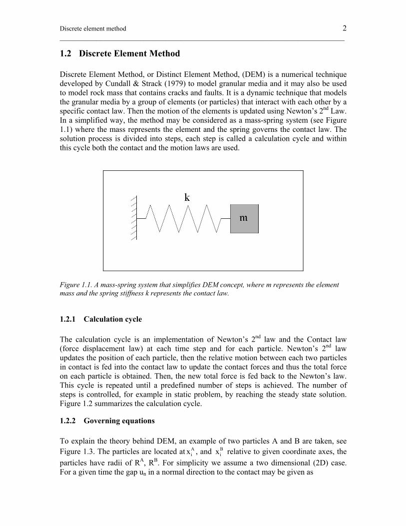
1.2 Discrete Element Method Discrete Element Method, or Distinct Element Method, (DEM) is a numerical technique developed by Cundall & Strack (1979) to model granular media and it may also be used to model rock mass that contains cracks and faults. It is a dynamic technique that models the granular media by a group of elements (or particles) that interact with each other by a specific contact law. Then the motion of the elements is updated using Newton’s 2nd Law. In a simplified way, the method may be considered as a mass-spring system (see Figure 1.1) where the mass represents the element and the spring governs the contact law. The solution process is divided into steps, each step is called a calculation cycle and within this cycle both the contact and the motion laws are used.
Figure 1.1. A mass-spring system that simplifies DEM concept, where m represents the element mass and the spring stiffness k represents the contact law.
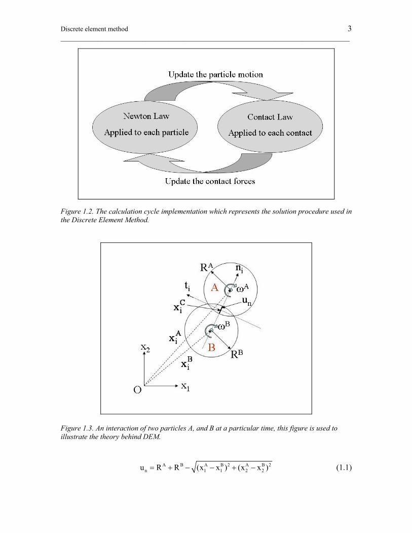
1.2.1 Calculation cycle The calculation cycle is an implementation of Newton’s 2nd law and the Contact law (force displacement law) at each time step and for each particle. Newton’s 2nd law updates the position of each particle, then the relative motion between each two particles in contact is fed into the contact law to update the contact forces and thus the total force on each particle is obtained. Then, the new total force is fed back to the Newton’s law. This cycle is repeated until a predefined number of steps is achieved. The number of steps is controlled, for example in static problem, by reaching the steady state solution. Figure 1.2 summarizes the calculation cycle.
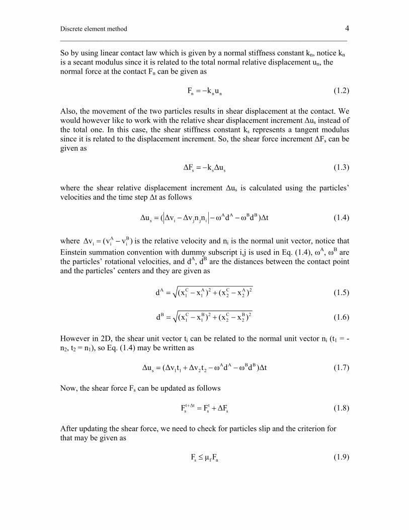
1.2.2 Governing equations To explain the theory behind DEM, an example of two particles A and B are taken, see Figure 1.3. The particles are located at A
ix , and Bix relative to given coordinate axes, the
particles have radii of RA, RB. For simplicity we assume a two dimensional (2D) case. For a given time the gap un in a normal direction to the contact may be given as
Discrete element method 3 ______________________________________________________________________________
Figure 1.2. The calculation cycle implementation which represents the solution procedure used in the Discrete Element Method.
Figure 1.3. An interaction of two particles A, and B at a particular time, this figure is used to illustrate the theory behind DEM. A B A B 2 A B 2
n 1 1 2 2u R R (x x ) (x x )= + − − + − (1.1)
Discrete element method 4 ______________________________________________________________________________
So by using linear contact law which is given by a normal stiffness constant kn, notice kn is a secant modulus since it is related to the total normal relative displacement un, the normal force at the contact Fn can be given as n n nF k u= − (1.2) Also, the movement of the two particles results in shear displacement at the contact. We would however like to work with the relative shear displacement increment Δus instead of the total one. In this case, the shear stiffness constant ks represents a tangent modulus since it is related to the displacement increment. So, the shear force increment ΔFs can be given as s s sΔF k Δu= − (1.3) where the shear relative displacement increment Δus is calculated using the particles’ velocities and the time step Δt as follows A A B B
s i j j iΔu (Δv Δv n n ω d ω d )Δt= − − − (1.4) where A B
i i iΔv (v v )= − is the relative velocity and ni is the normal unit vector, notice that Einstein summation convention with dummy subscript i,j is used in Eq. (1.4), ωA, ωB are the particles’ rotational velocities, and dA, dB are the distances between the contact point and the particles’ centers and they are given as A C A 2 C A 2
1 1 2 2d (x x ) (x x )= − + − (1.5) B C B 2 C B 2
1 1 2 2d (x x ) (x x )= − + − (1.6) However in 2D, the shear unit vector ti can be related to the normal unit vector ni (t1 = -n2, t2 = n1), so Eq. (1.4) may be written as A A B B
s 1 1 2 2Δu (Δv t Δv t ω d ω d )Δt= + − − (1.7) Now, the shear force Fs can be updated as follows t Δt t
s s sF F ΔF+ = + (1.8) After updating the shear force, we need to check for particles slip and the criterion for that may be given as s f nF μ F≤ (1.9)
Discrete element method 5 ______________________________________________________________________________
where μf is the friction coefficient between the two particles, and if Eq. (1.9) is violated the shear force is set to t Δt t Δt t
s f n sF μ F sign(F )+ += (1.10) After calculating Fn, and Fs at the contact C, the total contact force C
iF can be calculated as follows C
i n i s iF F n F t= + (1.11) This contact force will then be applied to the both particles as follows A C
i iF F= (1.12) B C
i iF F= − (1.13) The contact force C
iF will also cause moment M acting on the both particles which can be given as A C A C
3 jk j j kM e (x x )F= − (1.14) and B C B C
3 jk j j kM e (x x )F= − − (1.15) where eijk is the alternating tensor defined as
e123 = e231 = e312 = -e213 = -e132 = -e321 = 1, eijk = 0 otherwise.
It should be mentioned that in more realistic models, unlike the one shown in Figure 1.3, each particle will have more than one contact, so the contributions from all the contacts that lie on the same particle must be added to Eqs. (1.12) to (1.15). After getting the total force for each particle, we use Newton’s law to get the particle acceleration. Since we are still working with Figure 1.3, let us take particle A as an example. So the acceleration of particle A ( A
ia ) can be given as
A ex total
A i i ii A A
F F Fam m+
= = (1.16)
where mA is the particle mass, exiF is an external force applied to particle A, which can be
an act of gravity, pore pressure, or other type of loads defined by the user. Similarly, the rotational acceleration (αA) can be given a
A
AA
MαI
= (1.17)
Discrete element method 6 ______________________________________________________________________________
where IA is the moment of inertia of particle A, for example for a disk-shaped particle is given as
A A A 21I m (R )2
= (1.18)
After getting the values of the particle’s transitional and rotational accelerations, the values of the velocity and the rotational velocity can be updated using central-finite difference integration scheme as follows
Δt Δtt tA A A2 2
i i i(v ) (v ) a Δt+ −
= + (1.19) and
Δt Δtt tA A A2 2(ω ) (ω ) α Δt
+ −= + (1.20)
Finally, the particle’s position is updated as
ΔttA t Δt A t A 2
i i i(x ) (x ) (v ) Δt++ = + (1.21)
There are many other integration schemes that can be used instead of the above one, for example Munjiza (2004) lists many high-order schemes. Although these schemes can be more accurate than the above first-order one, they demand more computer memory and CPU time which is more costly in term of numerical modeling. Besides, the above scheme appears to be sufficient for our purpose, giving its simplicity and efficiency.
1.2.3 Mechanical damping Mechanical damping is a phenomenon inside the rocks that causes energy dissipation for example through fracturing or internal friction. Damping causes rocks, during mechanical loading, to reach the state of rest, or in numerical modeling term, the steady state solution. In DEM, damping may be applied to the particles as a viscous force acting on each contact which can be given as a function of shear and normal damping coefficients, cn, cs, as follows d
n n nF c Δv= (1.22) and d
s s sF c Δv= (1.23) where Δvn, Δvs, are the relative normal and shear velocities, respectively. These forces are then included in Eq. (1.11) as follows C d d
i n n i s s iF (F F )n (F F )t= − + − (1.24)
Discrete element method 7 ______________________________________________________________________________
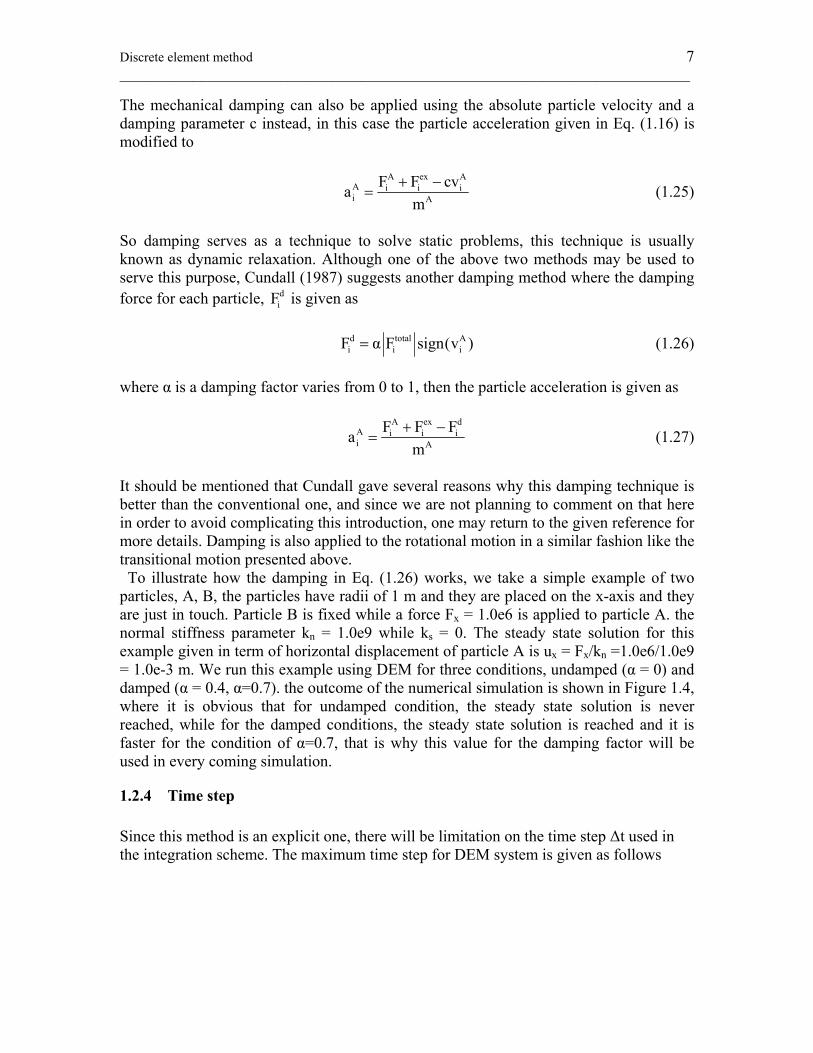
The mechanical damping can also be applied using the absolute particle velocity and a damping parameter c instead, in this case the particle acceleration given in Eq. (1.16) is modified to
A ex A
A i i ii A
F F cvam
+ −= (1.25)
So damping serves as a technique to solve static problems, this technique is usually known as dynamic relaxation. Although one of the above two methods may be used to serve this purpose, Cundall (1987) suggests another damping method where the damping force for each particle, d
iF is given as d total A
i i iF α F sign(v )= (1.26) where α is a damping factor varies from 0 to 1, then the particle acceleration is given as
A ex d
A i i ii A
F F Fam
+ −= (1.27)
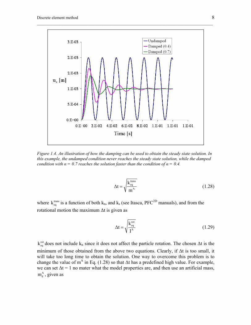
It should be mentioned that Cundall gave several reasons why this damping technique is better than the conventional one, and since we are not planning to comment on that here in order to avoid complicating this introduction, one may return to the given reference for more details. Damping is also applied to the rotational motion in a similar fashion like the transitional motion presented above. To illustrate how the damping in Eq. (1.26) works, we take a simple example of two particles, A, B, the particles have radii of 1 m and they are placed on the x-axis and they are just in touch. Particle B is fixed while a force Fx = 1.0e6 is applied to particle A. the normal stiffness parameter kn = 1.0e9 while ks = 0. The steady state solution for this example given in term of horizontal displacement of particle A is ux = Fx/kn =1.0e6/1.0e9 = 1.0e-3 m. We run this example using DEM for three conditions, undamped (α = 0) and damped (α = 0.4, α=0.7). the outcome of the numerical simulation is shown in Figure 1.4, where it is obvious that for undamped condition, the steady state solution is never reached, while for the damped conditions, the steady state solution is reached and it is faster for the condition of α=0.7, that is why this value for the damping factor will be used in every coming simulation.
1.2.4 Time step Since this method is an explicit one, there will be limitation on the time step Δt used in the integration scheme. The maximum time step for DEM system is given as follows
Discrete element method 8 ______________________________________________________________________________
Figure 1.4. An illustration of how the damping can be used to obtain the steady state solution. In this example, the undamped condition never reaches the steady state solution, while the damped condition with α = 0.7 reaches the solution faster than the condition of α = 0.4.
transeq
A
kΔt
m= (1.28)
where trans
eqk is a function of both kn, and ks (see Itasca, PFC2D manuals), and from the rotational motion the maximum Δt is given as
roteqA
kΔt
I= (1.29)
roteqk does not include kn since it does not affect the particle rotation. The chosen Δt is the
minimum of those obtained from the above two equations. Clearly, if Δt is too small, it will take too long time to obtain the solution. One way to overcome this problem is to change the value of mA in Eq. (1.28) so that Δt has a predefined high value. For example, we can set Δt = 1 no mater what the model properties are, and then use an artificial mass,
Adm , given as
Discrete element method 9 ______________________________________________________________________________
A transd eqm k= (1.30)
This mass is used in Eqs. (1.27) instead of the correct mass mA. Although using this artificial mass will speed up the simulation, the result is only valid for the steady state solution. This means that this technique can not be used for dynamic problems, but only for static problems.
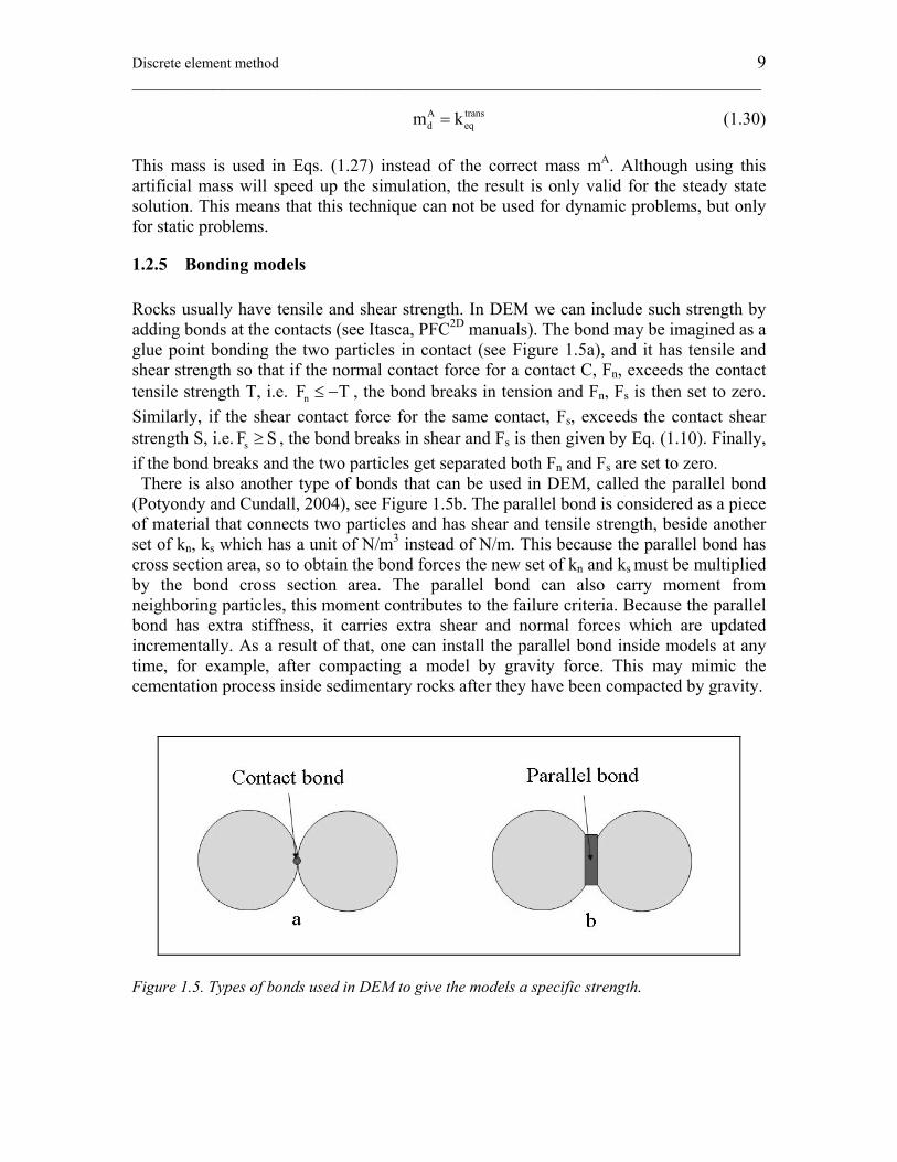
1.2.5 Bonding models Rocks usually have tensile and shear strength. In DEM we can include such strength by adding bonds at the contacts (see Itasca, PFC2D manuals). The bond may be imagined as a glue point bonding the two particles in contact (see Figure 1.5a), and it has tensile and shear strength so that if the normal contact force for a contact C, Fn, exceeds the contact tensile strength T, i.e. nF T≤ − , the bond breaks in tension and Fn, Fs is then set to zero. Similarly, if the shear contact force for the same contact, Fs, exceeds the contact shear strength S, i.e. sF S≥ , the bond breaks in shear and Fs is then given by Eq. (1.10). Finally, if the bond breaks and the two particles get separated both Fn and Fs are set to zero. There is also another type of bonds that can be used in DEM, called the parallel bond (Potyondy and Cundall, 2004), see Figure 1.5b. The parallel bond is considered as a piece of material that connects two particles and has shear and tensile strength, beside another set of kn, ks which has a unit of N/m3 instead of N/m. This because the parallel bond has cross section area, so to obtain the bond forces the new set of kn and ks must be multiplied by the bond cross section area. The parallel bond can also carry moment from neighboring particles, this moment contributes to the failure criteria. Because the parallel bond has extra stiffness, it carries extra shear and normal forces which are updated incrementally. As a result of that, one can install the parallel bond inside models at any time, for example, after compacting a model by gravity force. This may mimic the cementation process inside sedimentary rocks after they have been compacted by gravity.
Figure 1.5. Types of bonds used in DEM to give the models a specific strength.
Other numerical methods 10 ________________________________________________________________________
1.3 Other numerical methods Although this work is focusing on studying the possibilities for using DEM in reservoir geomechanics, it should be mentioned that there are other well-established methods that are currently used to model geomechanical behavior of hydrocarbon reservoirs. Such of these methods are, Finite Element and Finite Difference Methods (FEM & FDM). In this section, a brief introduction to those methods will be given to allows the reader to see the similarities and the differences between those methods and DEM.
1.3.1 Finite Element Method (FEM) The Finite Element Method (FEM) is used to solve partial differential equations by dividing a problem domain into several elements with specific shape (triangular, or rectangular). Then it uses a trial function (usually a simple one) as an approximation to the solution. The trial function works on each element. Since this approximation might be rough (depending on the trial function), increasing the number of elements in the domain will result in more accurate solution. There are several techniques used in FEM and the differences are usually based, for example, on what type of trial function is used. Some of those techniques (see Zienkiewicz et. al. 2000 & Kwon et. al. 1997) are Weighted Residual method, Energy Method, Rayleigh-Ritz Method, and Galerkin’s Method. In this section we will demonstrate the use of the last technique (Galerkin’s Method) to solve the problem of elastic solid, since this type of problem is encountered in reservoir geomechanics. So we start by writing the differential equations that describe the equilibrium of elastic solid and we limit our self by 2D problems as follows
xyxxx
σσ f 0x y
∂∂+ + =
∂ ∂ (1.31)
yy xyy
σ σf 0
y x∂ ∂
+ + =∂ ∂
(1.32)
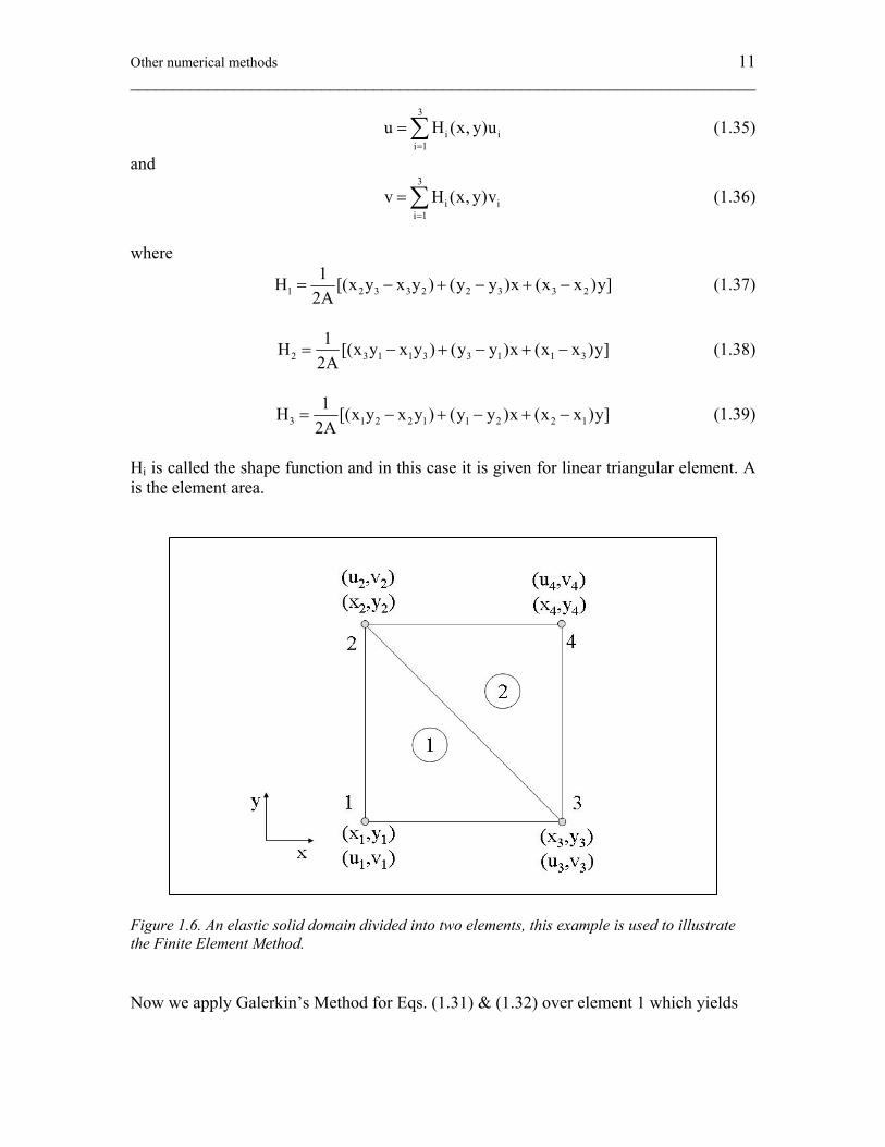
where σij are the stress tensors and fi are the body loads, i = x, y. let us assume that a domain we want to work on is a square and that it is divided into two triangular elements only, see Figure 1.6. Then a linear trial function is used to approximate the solution which is, in this case, given by a displacement field, u and v as follows 1 2 3u a a x a y= + + (1.33) 1 2 3v b b x b y= + + (1.34) For each element, Eqs. (1.33) & (1.34) can be written in term of nodal displacements of that element, for example, for element 1 in Figure 1.6 , one may write
Other numerical methods 11 ________________________________________________________________________
3
i ii 1
u H (x, y)u=
= ∑ (1.35)
and
3
i ii 1
v H (x, y)v=
= ∑ (1.36)
where
1 2 3 3 2 2 3 3 21H [(x y x y ) (y y )x (x x )y]
2A= − + − + − (1.37)
2 3 1 1 3 3 1 1 31H [(x y x y ) (y y )x (x x )y]
2A= − + − + − (1.38)
3 1 2 2 1 1 2 2 11H [(x y x y ) (y y )x (x x )y]
2A= − + − + − (1.39)
Hi is called the shape function and in this case it is given for linear triangular element. A is the element area.
Figure 1.6. An elastic solid domain divided into two elements, this example is used to illustrate the Finite Element Method. Now we apply Galerkin’s Method for Eqs. (1.31) & (1.32) over element 1 which yields
Other numerical methods 12 ________________________________________________________________________
32
1 1
xyxyxx
1 1 1 xy x
σσI [ω ( ) ω (f )] x y 0x y
∂∂= + + ∂ ∂ =
∂ ∂∫ ∫ (1.40)
and
32
1 1
xyyy xy
2 2 2 yy x
σ σI [ω ( ) ω (f )] x y 0
y x∂ ∂
= + + ∂ ∂ =∂ ∂∫ ∫ (1.41)
where ω1, ω2 are weighting functions and for the Galerkin’s Method are given as
1 ii
uω Hu
∂= =
∂ (1.42)
and
2 ii
vω Hv
∂= =
∂ (1.43)
Furthermore, to simplify the first parts of Eqs. (1.40) & (1.41), we use the Green’s theorem which may be proven by using integration by part and states that for two functions f (x, y), g (x, y) one may write
2 2 2 2
1 1 1 1
y x y x
xy x y x S
g ff x y g x y f g n Sx x
∂ ∂⋅ ⋅∂ ∂ = − ⋅ ⋅∂ ∂ + ⋅ ⋅ ⋅∂∂ ∂∫ ∫ ∫ ∫ ∫ (1.44)
The second term in the right-hand side of Eq. (1.44) represents the traction applied to the domain boundary S, this term is usually known as the Neuman boundary condition. Since in this example we are not planning to add any traction for simplicity reason, this part will be neglected. Now, we recall the following relations for the strain and the stress
xx xx
yy yy
xy xy
σ λ 2μ λ 0 εσ λ λ 2μ 0 εσ 0 0 μ ε
⎡ ⎤ ⎡ ⎤+⎡ ⎤⎢ ⎥ ⎢ ⎥⎢ ⎥= + =⎢ ⎥ ⎢ ⎥⎢ ⎥⎢ ⎥ ⎢ ⎥⎢ ⎥⎣ ⎦⎣ ⎦ ⎣ ⎦
Cε (1.45)
and
xx
yy
xy
uxεvεy
ε1 u v( )2 y x
⎡ ⎤∂⎢ ⎥
∂⎢ ⎥⎡ ⎤⎢ ⎥∂⎢ ⎥ = ⎢ ⎥⎢ ⎥ ∂⎢ ⎥⎢ ⎥⎣ ⎦ ⎢ ⎥∂ ∂
+⎢ ⎥∂ ∂⎣ ⎦
(1.46)
and by using Eqs. (1.35) & (1.36) we end up with
Other numerical methods 13 ________________________________________________________________________
131 2
1xx
231 2yy
2xy
33 31 1 2 2
3
uHH H0 0 vx x xεuHH Hε 0 0 0vy y y
εuH HH H H H
y x y x y x v
⎡ ⎤⎡ ⎤∂∂ ∂⎢ ⎥⎢ ⎥
∂ ∂ ∂ ⎢ ⎥⎢ ⎥⎡ ⎤⎢ ⎥⎢ ⎥∂∂ ∂⎢ ⎥ = =⎢ ⎥⎢ ⎥⎢ ⎥ ∂ ∂ ∂ ⎢ ⎥⎢ ⎥⎢ ⎥⎣ ⎦ ⎢ ⎥⎢ ⎥∂ ∂∂ ∂ ∂ ∂⎢ ⎥⎢ ⎥∂ ∂ ∂ ∂ ∂ ∂ ⎢ ⎥⎣ ⎦ ⎣ ⎦
eBU (1.47)
Also Eqs. (1.35) & (1.36) may be written in a matrix form as follows
1
1
1 2 3 2
1 2 3 2
3
3
uv
H 0 H 0 H 0 uu0 H 0 H 0 H vv
uv
⎡ ⎤⎢ ⎥⎢ ⎥⎢ ⎥⎡ ⎤⎡ ⎤
= =⎢ ⎥⎢ ⎥⎢ ⎥⎣ ⎦ ⎣ ⎦ ⎢ ⎥
⎢ ⎥⎢ ⎥⎢ ⎥⎣ ⎦
eNU (1.48)
Then we substitute Eqs. (1.42) to (1.44) into Eqs. (1.40) & (1.41), so we get
3 32 2
1 1 1 1
1 1xx xyx xy y
1 x
2 y2 2y x y xyy xy
ω ωσ σω fx y
x y x yω fω ωσ σ
y x
∂ ∂⎡ ⎤+⎢ ⎥ ⎡ ⎤∂ ∂⎢ ⎥∂ ∂ = ∂ ∂⎢ ⎥∂ ∂⎢ ⎥ ⎣ ⎦+⎢ ⎥∂ ∂⎣ ⎦
∫ ∫ ∫ ∫ (1.49)
By using Eqs. (1.45) to (1.48), Eq. (1.49) may be written as
3 32 2
1 1 1 1
x xy yx
yy x y x
f[ ] x y x y
f⎡ ⎤
∂ ∂ = ∂ ∂⎢ ⎥⎣ ⎦
∫ ∫ ∫ ∫T e TB CBU N (1.50)
and after applying the double integral, we end up with e e eK U =F (1.51) where Fe (the second term of Eq. (1.50)) is the nodal applied force for the element, and Ke = BTCBA is called the element stiffness matrix. This process is repeated for all the elements in the model (in this example only two elements), then a global stiffness matrix K is assembled such that the following set of linear equations is obtained KU=F (1.52)
Other numerical methods 14 ________________________________________________________________________
Finally, Eq. (1.52) is solved using algebra after applying the required load in F, and the required displacement constrain in U. Then, after obtaining the solution (represented by the nodal displacements U), the values of the stress and the strain can be calculated using the above equations.
1.3.2 Finite Difference Method The Finite Difference Method (FDM) is another common numerical method which is used to solve partial differential equations. Unlike FEM which depends on approximating the solution of the differential equation by a specific shape function, FDM depends on approximating the differential equation itself using Taylor’s expansion, for example. One of the advantages of FDM over FEM is the simplicity in deriving the solution, which of course will result in speeding up the solution time using computers. However, FDM uses structured mesh (usually rectangular grids) to cover the solution domain, and in some cases it is even difficult to have non-uniform grids size, which makes it difficult to solve problems that have domains of complex surfaces, that is why FEM is the method of choice in such problems. Yet in some problems, approximating the domain boundaries and interfaces with rectangular grids is considered a sufficient approximation, for example when simulating fluid flow in hydrocarbon reservoirs. Although FDM is considered an Eulerian method, because the solution inside each grid is changing while the grid itself remains fixed, another Lagragian type is also available which allows the use of unstructured, non-uniform grids. This type allows the grids to move with the solution, which makes it more suitable to solve problems of deforming solid, and since reservoir geomechanic is considered one of these problems, this type will be explained briefly downward, see Wilkins (1964) for more details. Let us start with Figure 1.7 which shows a grid made of 4 zones, each zone has 4 nodes. Now, at any time the equation of motion for a node, for example node a, may be written as (the zone stresses are applied as forces to each node using the zones’ edges)
t Δt t 1 t 2 ta a xx a e xx e a
a3 t 4 t 1 txx a d xx d a xy b a
2 t 3 t 4 txy a c xy c a xy a b
Δtx x [(σ ) (y y ) (σ ) (y y )m
(σ ) (y y ) (σ ) (y y ) (σ ) (x x )
(σ ) (x x ) (σ ) (x x ) (σ ) (x x )]
+ = − − + −
+ − + − − −
− − − − − −
(1.53)
and
t Δt t 1 t 2 ta a yy b a yy a c
a3 t 4 t 1 tyy c a yy a b xy a e
2 t 3 t 4 txy e a xy a d xy d a
Δty y [(σ ) (x x ) (σ ) (x x )m
(σ ) (x x ) (σ ) (x x ) (σ ) (y y )
(σ ) (y y ) (σ ) (y y ) (σ ) (y y )]
+ = − − + −
+ − + − − −
− − − − − −
(1.54)
where Δt is the time step, x, y are the node’s velocities, σij is the zones’ stress, and m is the node’s mass obtained form the conservation of mass equation. After obtaining the nodal velocities at the current time, the zones’ strain rate ijε for each zone ( say zone 1) can be updated as follows
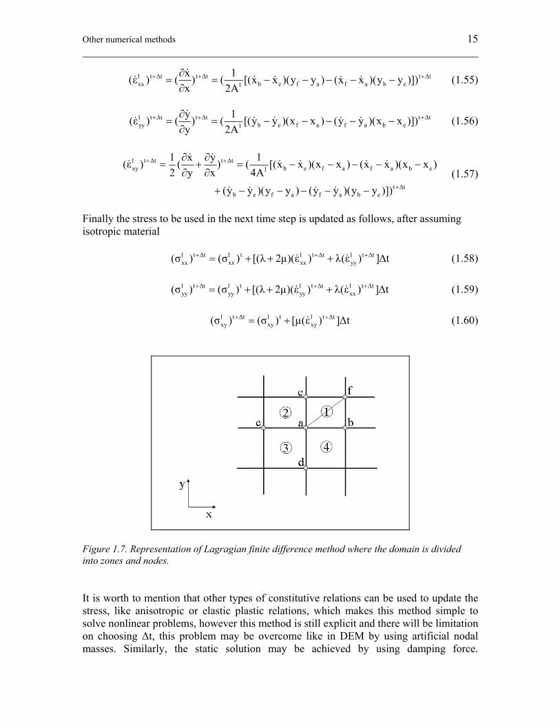
Other numerical methods 15 ________________________________________________________________________
1 t Δt t Δt t Δtxx b e f a f a b e1
x 1(ε ) ( ) ( [(x x )(y y ) (x x )(y y )])x 2A
+ + +∂= = − − − − −
∂ (1.55)
1 t Δt t Δt t Δtyy b e f a f a b e1
y 1(ε ) ( ) ( [(y y )(x x ) (y y )(x x )])y 2A
+ + +∂= = − − − − −
∂ (1.56)
1 t Δt t Δtxy b e f a f a b e1
t Δtb e f a f a b e
1 x y 1(ε ) ( ) ( [(x x )(x x ) (x x )(x x )2 y x 4A
(y y )(y y ) (y y )(y y )])
+ +
+
∂ ∂= + = − − − − −
∂ ∂
+ − − − − − (1.57)
Finally the stress to be used in the next time step is updated as follows, after assuming isotropic material 1 t Δt 1 t 1 t Δt 1 t Δt
xx xx xx yy(σ ) (σ ) [(λ 2μ)(ε ) λ(ε ) ]Δt+ + += + + + (1.58) 1 t Δt 1 t 1 t Δt 1 t Δt
yy yy yy xx(σ ) (σ ) [(λ 2μ)(ε ) λ(ε ) ]Δt+ + += + + + (1.59) 1 t Δt 1 t 1 t Δt
xy xy xy(σ ) (σ ) [μ(ε ) ]Δt+ += + (1.60)
Figure 1.7. Representation of Lagragian finite difference method where the domain is divided into zones and nodes. It is worth to mention that other types of constitutive relations can be used to update the stress, like anisotropic or elastic plastic relations, which makes this method simple to solve nonlinear problems, however this method is still explicit and there will be limitation on choosing Δt, this problem may be overcome like in DEM by using artificial nodal masses. Similarly, the static solution may be achieved by using damping force.
Reservoir geomechanics 16 ________________________________________________________________________
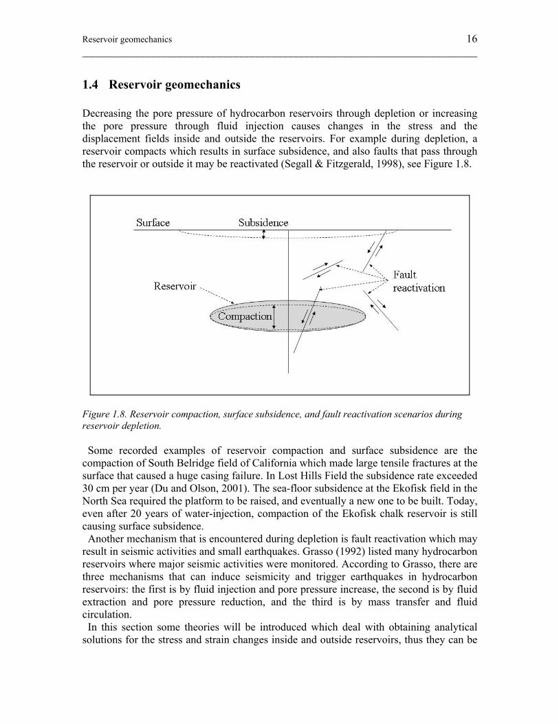
1.4 Reservoir geomechanics Decreasing the pore pressure of hydrocarbon reservoirs through depletion or increasing the pore pressure through fluid injection causes changes in the stress and the displacement fields inside and outside the reservoirs. For example during depletion, a reservoir compacts which results in surface subsidence, and also faults that pass through the reservoir or outside it may be reactivated (Segall & Fitzgerald, 1998), see Figure 1.8.
Figure 1.8. Reservoir compaction, surface subsidence, and fault reactivation scenarios during reservoir depletion. Some recorded examples of reservoir compaction and surface subsidence are the compaction of South Belridge field of California which made large tensile fractures at the surface that caused a huge casing failure. In Lost Hills Field the subsidence rate exceeded 30 cm per year (Du and Olson, 2001). The sea-floor subsidence at the Ekofisk field in the North Sea required the platform to be raised, and eventually a new one to be built. Today, even after 20 years of water-injection, compaction of the Ekofisk chalk reservoir is still causing surface subsidence. Another mechanism that is encountered during depletion is fault reactivation which may result in seismic activities and small earthquakes. Grasso (1992) listed many hydrocarbon reservoirs where major seismic activities were monitored. According to Grasso, there are three mechanisms that can induce seismicity and trigger earthquakes in hydrocarbon reservoirs: the first is by fluid injection and pore pressure increase, the second is by fluid extraction and pore pressure reduction, and the third is by mass transfer and fluid circulation. In this section some theories will be introduced which deal with obtaining analytical solutions for the stress and strain changes inside and outside reservoirs, thus they can be
Reservoir geomechanics 17 ________________________________________________________________________
used to calculate compaction and subsidence, also to study the possibilities of fault reactivation. Although those solutions are based on some simple assumptions, they can play a very significant rule in understanding a reservoir geomechanical response during fluid and stress change.
1.4.1 Nucleus of strain and Geertsma solution The differential equation that describes mechanical equilibrium of poroelastic media may be written as
2
j2i i
i j i
uμ Pμ u α f 0(1 2ν) x x x
∂ ∂∇ + − + =
− ∂ ∂ ∂ (1.61)
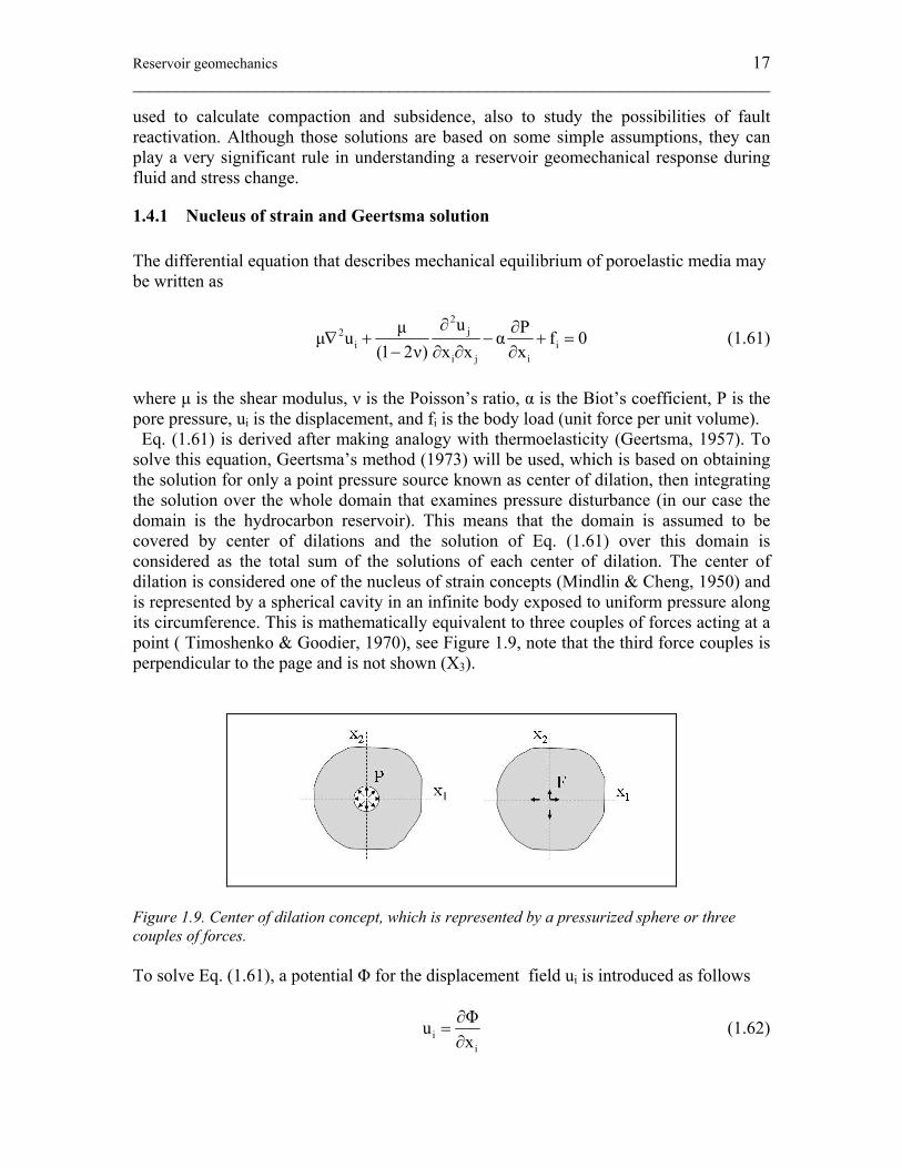
where μ is the shear modulus, ν is the Poisson’s ratio, α is the Biot’s coefficient, P is the pore pressure, ui is the displacement, and fi is the body load (unit force per unit volume). Eq. (1.61) is derived after making analogy with thermoelasticity (Geertsma, 1957). To solve this equation, Geertsma’s method (1973) will be used, which is based on obtaining the solution for only a point pressure source known as center of dilation, then integrating the solution over the whole domain that examines pressure disturbance (in our case the domain is the hydrocarbon reservoir). This means that the domain is assumed to be covered by center of dilations and the solution of Eq. (1.61) over this domain is considered as the total sum of the solutions of each center of dilation. The center of dilation is considered one of the nucleus of strain concepts (Mindlin & Cheng, 1950) and is represented by a spherical cavity in an infinite body exposed to uniform pressure along its circumference. This is mathematically equivalent to three couples of forces acting at a point ( Timoshenko & Goodier, 1970), see Figure 1.9, note that the third force couples is perpendicular to the page and is not shown (X3).
Figure 1.9. Center of dilation concept, which is represented by a pressurized sphere or three couples of forces. To solve Eq. (1.61), a potential Φ for the displacement field ui is introduced as follows
ii
Φux
∂=
∂ (1.62)
Reservoir geomechanics 18 ________________________________________________________________________
Then, by substituting Eq. (1.62) into Eq. (1.61) we end up with 2
mΦ c P∇ = (1.63) where cm is the uniaxial compaction coefficient and is given as
mα(1 2ν)c2μ(1 ν)
−=
− (1.64)
For a center of dilation located at point ξi, Eq. (1.63) becomes 2
m 1 1 2 2 3 3Φ c Pδ(x ξ )δ(x ξ )δ(x ξ )∇ = − − − (1.65) where δ(x) is the delta function, and the solution of Eq. (1.65) at any point x may be given as
1 1 2 2 3 3m1 2 3
δ(x ξ )δ(x ξ )δ(x ξ )c PΦ ξ ξ ξ4π R
− − −= − ∂ ∂ ∂∫∫∫ (1.66)
where 2 2 2
1 1 2 2 3 3R (x ξ ) (x ξ ) (x ξ )= − + − + − , and form Eq. (1.66) we get
mc PΦ4πR
= − (1.67)
Thus, based on Eq. (1.62) we obtain
m i ii 3
c P (x ξ )u4π R
−= (1.68)
This solution is only valid for infinite solid. However since we seek the solution for hydrocarbon reservoirs where a free surface exists, a solution for a semi-infinite solid is needed. Such a solution was derived by Mindlin & Cheng (1950) for a nucleus of strain in a thermoelastic media by assuming an imaginary nucleus of strain (center of dilation) on the opposite side of the free surface and at similar distance from it as the real one. Davies (2003) simplifies their solution so that the displacement for a semi-infinite solid
eiu can be written as a function of the displacements of the real iu∞ and the imaginary iu '∞
of the infinite solid as follows
e ii i i 3
3
u 'u u (3 4ν)u ' 2xx
∞∞ ∞ ∂
= + − +∂
(1.69)
where both iu∞ and iu '∞ can be obtained using Eq. (1.68) and if these expressions are substituted in Eq. (1.69) the Geertsma solution will be retrieved. However, since in this
Reservoir geomechanics 19 ________________________________________________________________________
thesis the study will focus on 2D problems, the above approach will be used to derive the solution for semi-infinite plane. In this case Eq. (1.65) reduces to 2
m 1 1 3 3Φ c Pδ(x ξ )δ(x ξ )∇ = − − (1.70) The solution for this equation can be given as (Timoshenko & Goodier, 1970),
m1 1 3 3 1 3
c PΦ δ(x ξ )δ(x ξ ) ln(R) ξ ξ2π
= − − ∂ ∂∫∫ (1.71)
where 2 2
1 1 3 3R (x ξ ) (x ξ )= − + − , and from Eq. (1.71) we get
mc PΦ ln(R)2π
= (1.72)
So the values of iu∞ and iu '∞ for infinite plane can be given as
m i ii 2
1
c P (x ξ )u2π R
∞ −= (1.73)
and
'
m i ii 2
2
c P (x ξ )u '2π R
∞ −= (1.74)
where 2 2
1 1 1 3 3R (x ξ ) (x ξ )= − + − and 2 22 1 1 3 3R (x ξ ) (x ξ )= − + + , then by substituting
Eqs. (1.73) & (1.74) into Eq. (1.69) and assuming x1 = x, x3 = z, we get
e 3 3 3 3mz 2 2 4
1 2 2
z ξ 4ν(z ξ ) (z 3ξ ) 4z(z ξ )c Pu [2π R R R
− + − + += + − (1.75)
e 1 3m 1 1x 2 2 4
1 2 2
4z(x ξ )(z ξ )c P (x ξ ) (x ξ )u [ (3 4ν)2π R R R
− +− −= + − − (1.76)
Then, by using Eqs. (1.45) & (1.46), expressions for the stresses can be obtained as follows (an expression for the shear stress σxz is not derived since it will not be used later)
2 3
e 3 3 3 3mz 2 2 4 4 6
1 2 1 2 2
2(z ξ ) 2(z ξ )(5z ξ ) 16z(z ξ )μc P 1 1σ [ ]2π R R R R R
− + − += − − − + (1.77)
2 3
e 3 3 3 3mx 2 2 4 4 6
1 2 1 2 2
2(z ξ ) 6(z ξ )(3z ξ ) 16z(z ξ )μc P 1 3σ [ ]2π R R R R R
− + − += − − + + − (1.78)
Reservoir geomechanics 20 ________________________________________________________________________
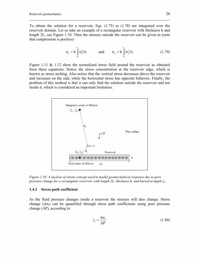
To obtain the solution for a reservoir, Eqs. (1.75) to (1.78) are integrated over the reservoir domain. Let us take an example of a rectangular reservoir with thickness h and length 2L, see Figure 1.10. Then the stresses outside the reservoir can be given as (note that compression is positive)
L L
e ez z x x
L L
σ h σ x and σ h σ x− −
= ∂ = ∂∫ ∫ (1.79)
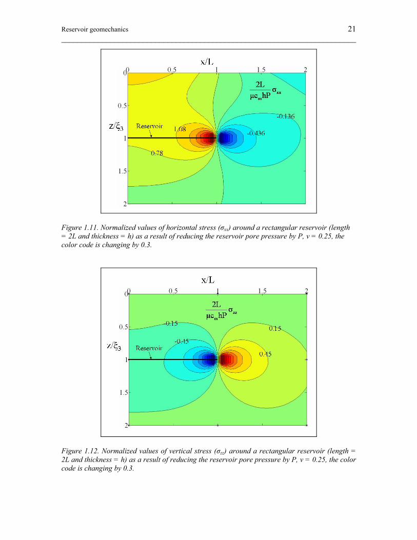
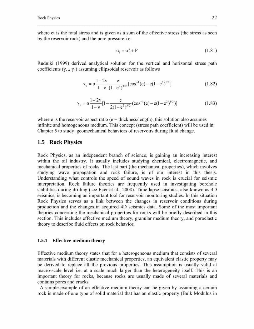
Figure 1.11 & 1.12 show the normalized stress field around the reservoir as obtained from these equations. Notice the stress concentration at the reservoir edge, which is known as stress arching. Also notice that the vertical stress decreases above the reservoir and increases on the side, while the horizontal stress has opposite behavior. Finally, the problem of this method is that it can only find the solution outside the reservoir and not inside it, which is considered an important limitation.
Figure 1.10. A nucleus of strain concept used to model geomechanical response due to pore pressure change for a rectangular reservoir with length 2L, thickness h, and buried at depth ξ3.
1.4.2 Stress path coefficient As the fluid pressure changes inside a reservoir the stresses will also change. Stress change (Δσi) can be quantified through stress path coefficients using pore pressure change (ΔP), according to
ii
σγΔPΔ
= (1.80)
Reservoir geomechanics 21 ________________________________________________________________________
Figure 1.11. Normalized values of horizontal stress (σxx) around a rectangular reservoir (length = 2L and thickness = h) as a result of reducing the reservoir pore pressure by P, ν = 0.25, the color code is changing by 0.3.
Figure 1.12. Normalized values of vertical stress (σzz) around a rectangular reservoir (length = 2L and thickness = h) as a result of reducing the reservoir pore pressure by P, ν = 0.25, the color code is changing by 0.3.
Rock Physics 22 ________________________________________________________________________
where σi is the total stress and is given as a sum of the effective stress (the stress as seen by the reservoir rock) and the pore pressure i.e. i iσ σ ' P= + (1.81) Rudniki (1999) derived analytical solution for the vertical and horizontal stress path coefficients (γv & γh) assuming ellipsoidal reservoir as follows
1 2 1/2v 2 3/2
1 2ν eγ α [cos (e) e(1 e ) ]1 ν (1 e )
−−= − −
− − (1.82)
1 2 1/2h 2 3/2
1 2ν eγ α [1 (cos (e) e(1 e ) )]1 ν 2(1 e )
−−= − − −
− − (1.83)
where e is the reservoir aspect ratio (e = thickness/length), this solution also assumes infinite and homogeneous medium. This concept (stress path coefficient) will be used in Chapter 5 to study geomechanical behaviors of reservoirs during fluid change.
1.5 Rock Physics Rock Physics, as an independent branch of science, is gaining an increasing interest within the oil industry. It usually includes studying chemical, electromagnetic, and mechanical properties of rocks. The last part (the mechanical properties), which involves studying wave propagation and rock failure, is of our interest in this thesis. Understanding what controls the speed of sound waves in rock is crucial for seismic interpretation. Rock failure theories are frequently used in investigating borehole stabilities during drilling (see Fjær et al., 2008). Time lapse seismics, also known as 4D seismics, is becoming an important tool for reservoir monitoring studies. In this situation Rock Physics serves as a link between the changes in reservoir conditions during production and the changes in acquired 4D seismics data. Some of the most important theories concerning the mechanical properties for rocks will be briefly described in this section. This includes effective medium theory, granular medium theory, and poroelastic theory to describe fluid effects on rock behavior.
1.5.1 Effective medium theory Effective medium theory states that for a heterogeneous medium that consists of several materials with different elastic mechanical properties, an equivalent elastic property may be derived to replace all the previous properties. This assumption is usually valid at macro-scale level i.e. at a scale much larger than the heterogeneity itself. This is an important theory for rocks, because rocks are usually made of several materials and contains pores and cracks. A simple example of an effective medium theory can be given by assuming a certain rock is made of one type of solid material that has an elastic property (Bulk Modulus in
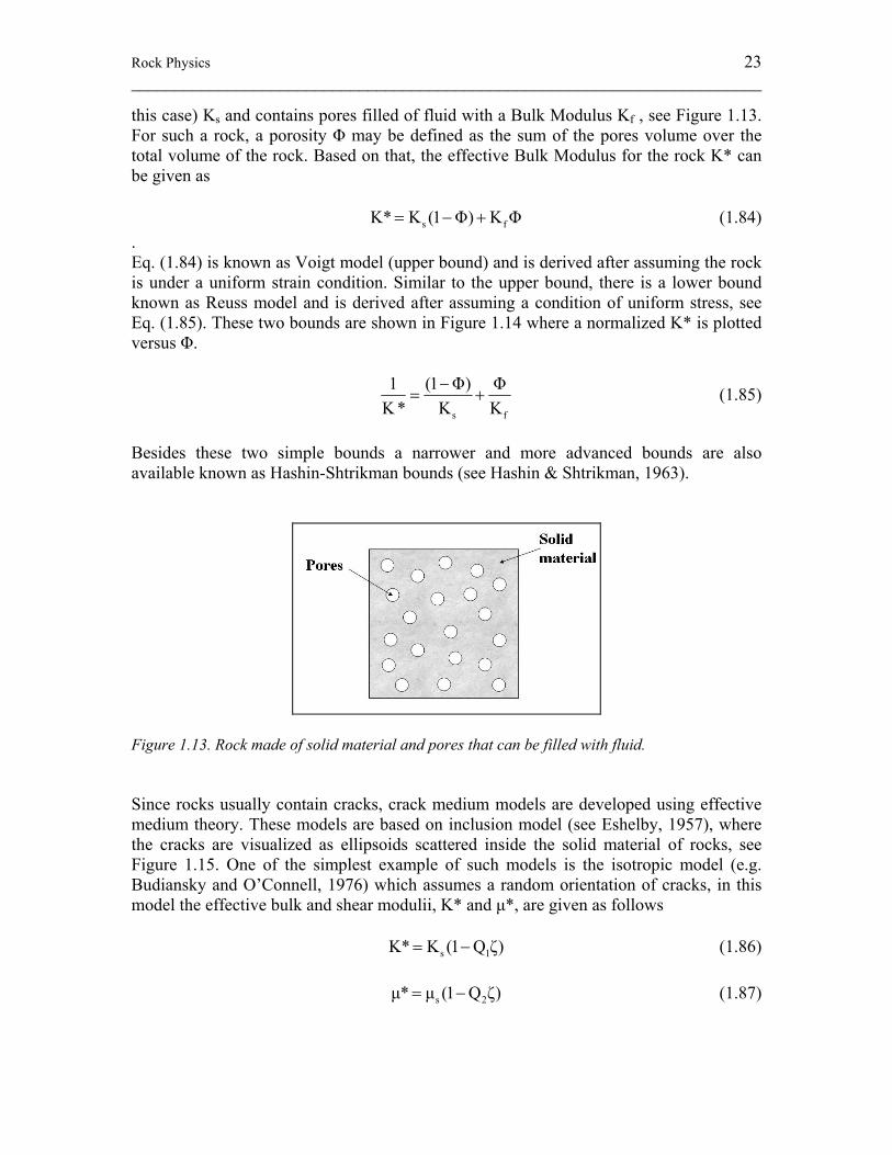
Rock Physics 23 ________________________________________________________________________
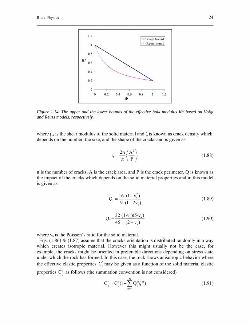
this case) Ks and contains pores filled of fluid with a Bulk Modulus Kf , see Figure 1.13. For such a rock, a porosity Φ may be defined as the sum of the pores volume over the total volume of the rock. Based on that, the effective Bulk Modulus for the rock K* can be given as s fK* K (1 Φ) K Φ= − + (1.84) . Eq. (1.84) is known as Voigt model (upper bound) and is derived after assuming the rock is under a uniform strain condition. Similar to the upper bound, there is a lower bound known as Reuss model and is derived after assuming a condition of uniform stress, see Eq. (1.85). These two bounds are shown in Figure 1.14 where a normalized K* is plotted versus Φ.
s f
1 (1 Φ) ΦK * K K
−= + (1.85)
Besides these two simple bounds a narrower and more advanced bounds are also available known as Hashin-Shtrikman bounds (see Hashin & Shtrikman, 1963).
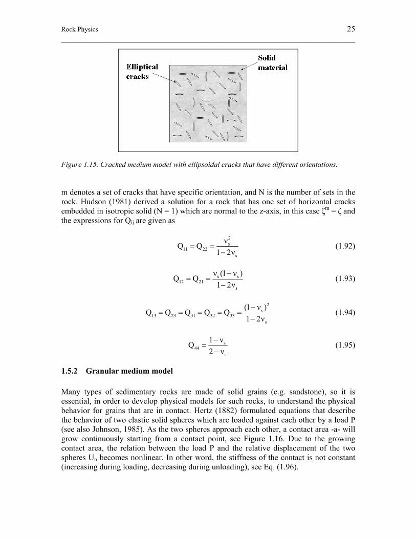
Figure 1.13. Rock made of solid material and pores that can be filled with fluid. Since rocks usually contain cracks, crack medium models are developed using effective medium theory. These models are based on inclusion model (see Eshelby, 1957), where the cracks are visualized as ellipsoids scattered inside the solid material of rocks, see Figure 1.15. One of the simplest example of such models is the isotropic model (e.g. Budiansky and O’Connell, 1976) which assumes a random orientation of cracks, in this model the effective bulk and shear modulii, K* and μ*, are given as follows s 1K* K (1 Q ζ)= − (1.86) s 2μ* μ (1 Q ζ)= − (1.87)
Rock Physics 24 ________________________________________________________________________
Figure 1.14. The upper and the lower bounds of the effective bulk modulus K* based on Voigt and Reuss models, respectively. where μs is the shear modulus of the solid material and ζ is known as crack density which depends on the number, the size, and the shape of the cracks and is given as
22n Aζ
π P= (1.88)
n is the number of cracks, A is the crack area, and P is the crack perimeter. Q is known as the impact of the cracks which depends on the solid material properties and in this model is given as
2s
1s
(1 ν )16Q9 (1 2ν )
−=
− (1.89)
s s2
s
(1-ν )(5-ν )32Q =45 (2 ν )−
(1.90)
where νs is the Poisson’s ratio for the solid material. Eqs. (1.86) & (1.87) assume that the cracks orientation is distributed randomly in a way which creates isotropic material. However this might usually not be the case, for example, the cracks might be oriented in preferable directions depending on stress state under which the rock has formed. In this case, the rock shows anisotropic behavior where the effective elastic properties *
ijC may be given as a function of the solid material elastic
properties sijC as follows (the summation convention is not considered)
N
* s m mij ij ij
m 1C C (1 Q ζ )
=
= −∑ (1.91)
Rock Physics 25 ________________________________________________________________________
Figure 1.15. Cracked medium model with ellipsoidal cracks that have different orientations. m denotes a set of cracks that have specific orientation, and N is the number of sets in the rock. Hudson (1981) derived a solution for a rock that has one set of horizontal cracks embedded in isotropic solid (N = 1) which are normal to the z-axis, in this case ζm = ζ and the expressions for Qij are given as
2s
11 22s
νQ Q1 2ν
= =−
(1.92)
s s12 21
s
ν (1 ν )Q Q1 2ν
−= =
− (1.93)
2
s13 23 31 32 33
s
(1 ν )Q Q Q Q Q1 2ν
−= = = = =
− (1.94)
s44
s
1 νQ2 ν
−=
− (1.95)
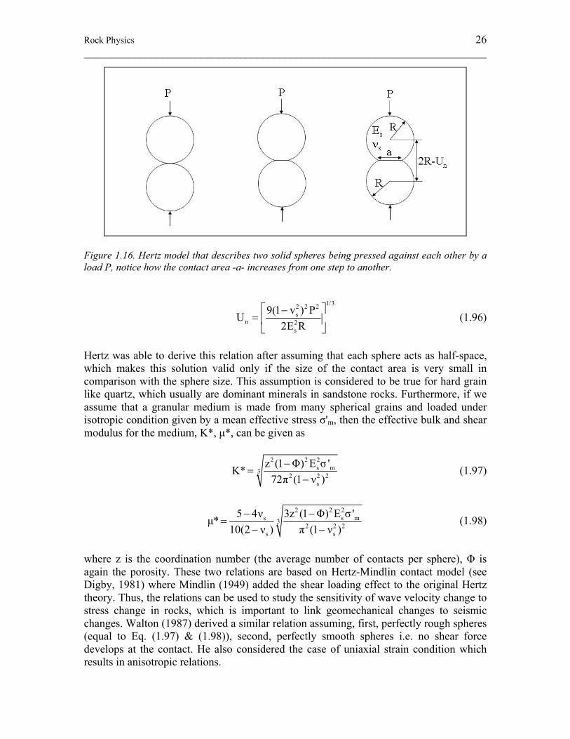
1.5.2 Granular medium model Many types of sedimentary rocks are made of solid grains (e.g. sandstone), so it is essential, in order to develop physical models for such rocks, to understand the physical behavior for grains that are in contact. Hertz (1882) formulated equations that describe the behavior of two elastic solid spheres which are loaded against each other by a load P (see also Johnson, 1985). As the two spheres approach each other, a contact area -a- will grow continuously starting from a contact point, see Figure 1.16. Due to the growing contact area, the relation between the load P and the relative displacement of the two spheres Un becomes nonlinear. In other word, the stiffness of the contact is not constant (increasing during loading, decreasing during unloading), see Eq. (1.96).
Rock Physics 26 ________________________________________________________________________
Figure 1.16. Hertz model that describes two solid spheres being pressed against each other by a load P, notice how the contact area -a- increases from one step to another.
1/32 2 2
sn 2
s
9(1 v ) PU2E R
⎡ ⎤−= ⎢ ⎥
⎣ ⎦ (1.96)
Hertz was able to derive this relation after assuming that each sphere acts as half-space, which makes this solution valid only if the size of the contact area is very small in comparison with the sphere size. This assumption is considered to be true for hard grain like quartz, which usually are dominant minerals in sandstone rocks. Furthermore, if we assume that a granular medium is made from many spherical grains and loaded under isotropic condition given by a mean effective stress σ'm, then the effective bulk and shear modulus for the medium, K*, μ*, can be given as
2 2 2
s m32 2 2
s
z (1 Φ) E σ 'K*72π (1 ν )
−=
− (1.97)
2 2 2
s s m32 2 2
s s
5 4ν 3z (1 Φ) E σ 'μ*10(2 ν ) π (1 ν )
− −=
− − (1.98)
where z is the coordination number (the average number of contacts per sphere), Φ is again the porosity. These two relations are based on Hertz-Mindlin contact model (see Digby, 1981) where Mindlin (1949) added the shear loading effect to the original Hertz theory. Thus, the relations can be used to study the sensitivity of wave velocity change to stress change in rocks, which is important to link geomechanical changes to seismic changes. Walton (1987) derived a similar relation assuming, first, perfectly rough spheres (equal to Eq. (1.97) & (1.98)), second, perfectly smooth spheres i.e. no shear force develops at the contact. He also considered the case of uniaxial strain condition which results in anisotropic relations.
Rock Physics 27 ________________________________________________________________________
1.5.3 Fluid effect The mechanical fluid effect on effective elastic properties of rocks is described by the poroelasticity theory, (see Biot, 1941 & 1962). The poroelasticity theory is based on macroscopic thermodynamics and hence neglects the shape of the pores in rocks and only looks to the fraction of the pore volume to the total volume of the rocks, which is usually known as a porosity Φ. One of the most significant equations in poroelasticity is the Biot-Gassmann equation, which enables us to estimate the contribution of the pore fluid stiffness to the total untrained stiffness of the rock. The equation defines the effective bulk modulus K* for a saturated rock made of a solid material with bulk modulus Ks, rock porosity Φ, and pore fluid stiffness kf as follows
2fr
sffr
f fr
s s
K(1 )KkK* K k KΦ 1 (1 Φ )
ΦK K
−= +
+ − − (1.99)
where Kfr is the framework (drained) bulk modulus for the rock i.e. the dry rock bulk modulus. This can be seen through Eq. (1.99), when there is no fluid in the rock (kf = 0), K* = Kfr. This equation assumes isotropic rock, monomineralic solid, and the fluid has no chemical effect on the framework bulk modulus. Notice that Kfr may be obtained from previous theory described above, or from mechanical test on a dry sample. On the other hand, poroelasticity theory shows no effect of the pore fluid on the shear modulus i.e. frμ* μ= (1.100) Eq. (1.99) is very important in estimating the effect of fluid substitution process inside a hydrocarbon reservoir during production on the stiffness property of the reservoir rock. Thus, it can serve as a link between saturation changes and seismic changes during reservoir monitoring studies.
1.6 Time-lapse seismics (4D seismics) Among other hydrocarbon reservoir monitoring techniques, time-lapse seismics (also known as 4D seismics) has emerged as a powerful reservoir monitoring tool (see e.g. Lumley, 2001). Some early successful studies of reservoir monitoring using 4D seismics showed its great potential. Such studies are, for example, Gullfaks field (Sønneland et al., 1997), and Fulmar field (Johnston et al., 1998) in the North Sea. The focus of those studies was to detect water-flushed zones by looking to seismic amplitude changes for the reservoir reflectors. By tracing the water movement and possible changes in oil-water contact (OWC), decision can be made for infill drilling to produce from bypass zones where no water flooding occurs. Not all reservoirs are suitable for 4D seismics monitoring. Therefore a feasibility study must be carried out before starting acquiring more seismic data. Lumley et al. (1997)
Time-lapse seismics 28 ________________________________________________________________________
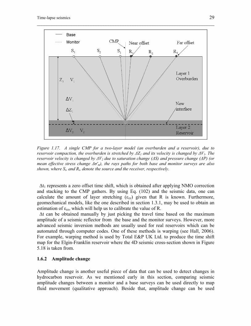
presented a technical risk spreadsheet which can be used to assess a reservoir potential for a time-lapse seismics study. The spread sheet includes several reservoir properties such as: fluid saturation, reservoir rock bulk modulus and porosity. For example, if a reservoir rock is stiff (high bulk modulus such as carbonate reservoir), detecting fluid change will be difficult. This can be explained by looking at Eq. (1.99), where if Kfr >> kf then K* ≈ Kfr regardless of fluid substitution during production. Another key point in time-lapse seismic study assessment is seismic repeatability issue. This means that the conditions of acquiring and processing a monitor seismic survey has to be similar to those of a base survey, so that the changes between the base and the monitor surveys are guaranteed to be only production-related and are not due to some seismic noise. Such factors that may affect seismic repeatability are; sea tides, changes in sea water temperature, noise from passing ships …etc. Marine seismic data can be acquired by two methods: Towed Seismic Streamer where a marine vessel pulls the hydrophones (receivers) line, or by Ocean Bottom Cable (OBC) where the receivers are installed on the sea floor. The second method has the advantage of recording S-wave as well as P-wave, however it is more expensive. The seismic data are, then, processed into common-midpoint (CMP) gathers, a most widely used processing technique. CMP concept will be used in the coming discussion. There are usually two ways used to exploit 4D seismics data, time shift and amplitude change. The following example will be used to explain those two ways briefly. Figure 1.17 shows a model made of two homogeneous layers, the upper layer represents the overburden and the lower layer represents the reservoir. Rays paths for a single CMP gather are also shown in the figure. Let us assume that the reservoir has been depleted, which causes saturation and pore pressure changes inside the reservoir, thus the velocity will increase. On the other hand, the reservoir compaction causes the overburden to stretch, which results in increasing the upper layer thickness and decreasing its velocity. The change in the upper layer thickness and velocity are denoted as; ΔZ1 and ΔV1, while the change in the lower layer velocity is ΔV2.
1.6.1 Time shift The change in ray path travel time between a monitor and a base surveys (see Figure 1.17) is called a time shift Δt. Landrø et al. (2004) shows that the time shift in a layer (say layer 1) Δt1 can be approximated as a function of the layer thickness change ΔZ1 and the velocity change ΔV1 as follows
1 1 1
1 1 1
Δt ΔZ ΔVt Z V
= − (1.101)
Hatchell et al. (2005) shows that Eq. (1.101) may be rewritten as follows
1zz
1
Δt (1 R)εt
= + (1.102)
where εzz = ΔZ1/Z1 is the vertical strain caused by layer stretching, R is a constant which relates ΔV1 to εzz by ΔV1/V1 = -Rεzz.
Time-lapse seismics 29 ________________________________________________________________________
Figure 1.17. A single CMP for a two-layer model (an overburden and a reservoir), due to reservoir compaction, the overburden is stretched by ΔZ1 and its velocity is changed by ΔV1. The reservoir velocity is changed by ΔV2 due to saturation change (ΔS) and pressure change (ΔP) (or mean effective stress change Δσ'm), the rays paths for both base and monitor surveys are also shown, where Si, and Ri, denote the source and the receiver, respectively. Δt1 represents a zero offset time shift, which is obtained after applying NMO correction and stacking to the CMP gathers. By using Eq. (102) and the seismic data, one can calculate the amount of layer stretching (εzz) given that R is known. Furthermore, geomechanical models, like the one described in section 1.3.1, may be used to obtain an estimation of εzz, which will help us to calibrate the value of R. Δt can be obtained manually by just picking the travel time based on the maximum amplitude of a seismic reflector from the base and the monitor surveys. However, more advanced seismic inversion methods are usually used for real reservoirs which can be automated through computer codes. One of these methods is warping (see Hall, 2006). For example, warping method is used by Total E&P UK Ltd. to produce the time shift map for the Elgin-Franklin reservoir where the 4D seismic cross-section shown in Figure 5.18 is taken from.
1.6.2 Amplitude change Amplitude change is another useful piece of data that can be used to detect changes in hydrocarbon reservoir. As we mentioned early in this section, comparing seismic amplitude changes between a monitor and a base surveys can be used directly to map fluid movement (qualitative approach). Beside that, amplitude change can be used
Time-lapse seismics 30 ________________________________________________________________________
quantitatively to discriminate between pressure and saturation changes for a given reservoir using AVO (Amplitude Versus Offset) analysis (see Landrø, 2001). Let us take the reservoir reflector that separate layer 1 and layer 2 shown in Figure 1.17 as an example. The amplitude change versus offset ΔRθ can be given using the AVO equation as follows 2
θ 0ΔR ΔR ΔG sin θ= + (1.103) where ΔR0 is AVO intersect (represents the zero offset amplitude change) and ΔG is the AVO gradient change, θ is the incident angle. The values of ΔR0 and ΔG can be obtained from near and far offset CMP gathers of 4D seismic data, see figure 1.17. Landrø (2001) shows that by using the values of ΔR0 and ΔG, one can write explicit expressions for fluid saturation and pore pressure changes (ΔS & ΔP) based on some Rock Physics models. It should be mentioned that Landrø (2001) assumed that the pressure change is equal to the mean effective stress change (ΔP = Δσ'm ), which is, according to Eq. (1.80), not necessary true, that is one of the reasons why reservoir geomechanic is needed in reservoir monitoring studies.

Chapter 2: Discrete element modeling 31 ________________________________________________________________________
2 Discrete element modeling of stress and strain evolution within and outside a depleting reservoir
*Published in Pure and Applied Geophysics. by Haitham Alassi, Rune Holt, and Liming Li. Vol. 163: 1-21, 2006.
2.1 Introduction Petroleum reservoir depletion leads to stress alteration within and outside the reservoir. During recent years it has become evident that such stress changes can have a profound impact on reservoir management (e.g., Teufel et al., 1991; Addis,1997; Kenter et al., 1998; Holt et al., 2004). Not only do they control purely mechanical deformation (reservoir compaction and surface subsidence), but they also impact petroleum recovery through compaction drive and through possible permeability changes. Furthermore, stress changes may affect the ability to drill stable wells, and the risks for onset of particle production or casing collapse throughout the life of the reservoir. In some cases, depletion-induced stress changes may be large enough to cause seismicity by activation of existing or generation of new faults. This may be utilized as a tool for reservoir performance monitoring (Maxwell and Urbancic, 2001). The main purpose of reservoir monitoring is to identify which parts of the reservoir that are produced, so that the production strategy can be tailored to the behavior of the reservoir. Today reservoirs are frequently monitored by ‘‘4-D’’ (also called time-lapse) seismics surveys. Clearly, stress sensitive wave velocities within a depleting reservoir or its surroundings may cause time-shifts that can be used as indicators of reservoir performance (Kenter et al., 2004). The economic impact of the issues above calls for modeling tools that can predict the evolution of stresses as a result of pore pressure changes associated with fluid extraction from the reservoir. Further, models need to be available that can also predict associated strains (compaction, subsidence, casing deformations), associated seismic velocity changes, and associated seismicity risk. There is currently no model that can be used to predict all these facets of the problem. Geomechanical simulators (Pande et al., 1990; Zienkiewicz, 1991; Jing and Hudson, 2002) addressing large scale problems like those described above are most often based on Finite Element (FEM) formulations, and are inherently static in the sense that they do not predict dynamic features like faulting. They do however predict plastic strain occurrence, but need to be re meshed in order to account for faulting. Although full poromechanical coupling is available (Settari and Mourits, 1994; Gutierrez and Lewis, 1998; Lewis et al., 2003; Koutsabeloulis and Hope, 1998; Osorio et al., 1998; Longuemare et al., 2002) in such models, at least in a staggered manner, a further link to seismic modeling is as yet absent. The motivation behind the work presented here is to explore the feasibility of applying an inherently dynamic model to this problem, namely a discrete element (DEM) approach. The DEM used here is the Particle Flow Code (PFC), which is available in 2-D and 3-D formulations, and which has been applied with success at grain scale (Cundall and Strack, 1979; Potyondy and Cundall, 2004), and also has been refined to incorporate poromechanical coupling (Shimizu, 2004; Li and Holt, 2004) and elastic wave
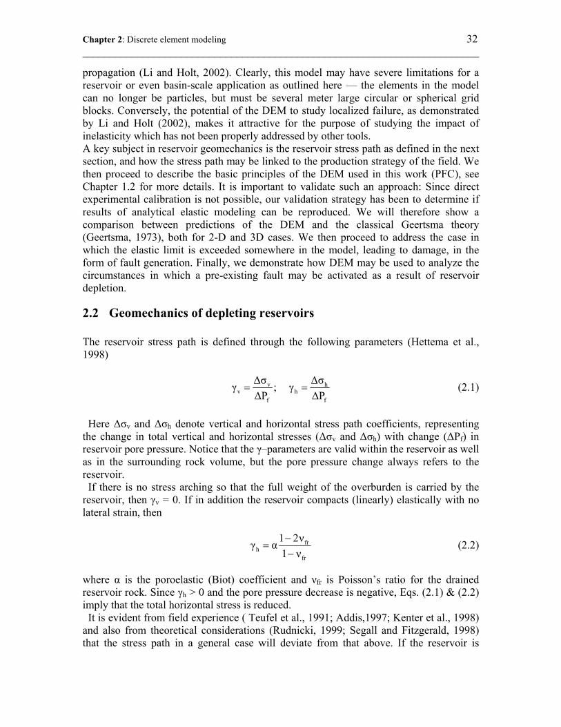
Chapter 2: Discrete element modeling 32 ________________________________________________________________________
propagation (Li and Holt, 2002). Clearly, this model may have severe limitations for a reservoir or even basin-scale application as outlined here — the elements in the model can no longer be particles, but must be several meter large circular or spherical grid blocks. Conversely, the potential of the DEM to study localized failure, as demonstrated by Li and Holt (2002), makes it attractive for the purpose of studying the impact of inelasticity which has not been properly addressed by other tools. A key subject in reservoir geomechanics is the reservoir stress path as defined in the next section, and how the stress path may be linked to the production strategy of the field. We then proceed to describe the basic principles of the DEM used in this work (PFC), see Chapter 1.2 for more details. It is important to validate such an approach: Since direct experimental calibration is not possible, our validation strategy has been to determine if results of analytical elastic modeling can be reproduced. We will therefore show a comparison between predictions of the DEM and the classical Geertsma theory (Geertsma, 1973), both for 2-D and 3D cases. We then proceed to address the case in which the elastic limit is exceeded somewhere in the model, leading to damage, in the form of fault generation. Finally, we demonstrate how DEM may be used to analyze the circumstances in which a pre-existing fault may be activated as a result of reservoir depletion.
2.2 Geomechanics of depleting reservoirs The reservoir stress path is defined through the following parameters (Hettema et al., 1998)
v hv h
f f
Δσ Δσγ ; γΔP ΔP
= = (2.1)
Here Δσv and Δσh denote vertical and horizontal stress path coefficients, representing the change in total vertical and horizontal stresses (Δσv and Δσh) with change (ΔPf) in reservoir pore pressure. Notice that the γ–parameters are valid within the reservoir as well as in the surrounding rock volume, but the pore pressure change always refers to the reservoir. If there is no stress arching so that the full weight of the overburden is carried by the reservoir, then γv = 0. If in addition the reservoir compacts (linearly) elastically with no lateral strain, then
frh
fr
1 2νγ α1 ν−
=−
(2.2)
where α is the poroelastic (Biot) coefficient and νfr is Poisson’s ratio for the drained reservoir rock. Since γh > 0 and the pore pressure decrease is negative, Eqs. (2.1) & (2.2) imply that the total horizontal stress is reduced. It is evident from field experience ( Teufel et al., 1991; Addis,1997; Kenter et al., 1998) and also from theoretical considerations (Rudnicki, 1999; Segall and Fitzgerald, 1998) that the stress path in a general case will deviate from that above. If the reservoir is
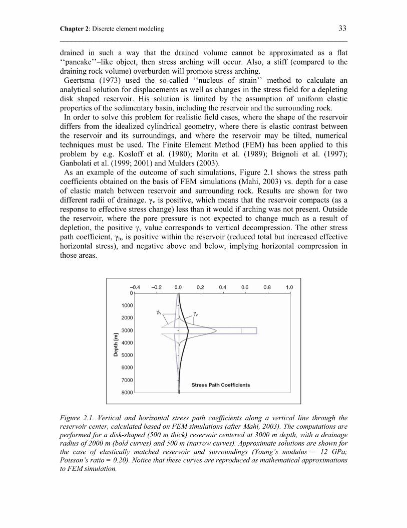
Chapter 2: Discrete element modeling 33 ________________________________________________________________________
drained in such a way that the drained volume cannot be approximated as a flat ‘‘pancake’’–like object, then stress arching will occur. Also, a stiff (compared to the draining rock volume) overburden will promote stress arching. Geertsma (1973) used the so-called ‘‘nucleus of strain’’ method to calculate an analytical solution for displacements as well as changes in the stress field for a depleting disk shaped reservoir. His solution is limited by the assumption of uniform elastic properties of the sedimentary basin, including the reservoir and the surrounding rock. In order to solve this problem for realistic field cases, where the shape of the reservoir differs from the idealized cylindrical geometry, where there is elastic contrast between the reservoir and its surroundings, and where the reservoir may be tilted, numerical techniques must be used. The Finite Element Method (FEM) has been applied to this problem by e.g. Kosloff et al. (1980); Morita et al. (1989); Brignoli et al. (1997); Ganbolati et al. (1999; 2001) and Mulders (2003). As an example of the outcome of such simulations, Figure 2.1 shows the stress path coefficients obtained on the basis of FEM simulations (Mahi, 2003) vs. depth for a case of elastic match between reservoir and surrounding rock. Results are shown for two different radii of drainage. γv is positive, which means that the reservoir compacts (as a response to effective stress change) less than it would if arching was not present. Outside the reservoir, where the pore pressure is not expected to change much as a result of depletion, the positive γv value corresponds to vertical decompression. The other stress path coefficient, γh, is positive within the reservoir (reduced total but increased effective horizontal stress), and negative above and below, implying horizontal compression in those areas.
Figure 2.1. Vertical and horizontal stress path coefficients along a vertical line through the reservoir center, calculated based on FEM simulations (after Mahi, 2003). The computations are performed for a disk-shaped (500 m thick) reservoir centered at 3000 m depth, with a drainage radius of 2000 m (bold curves) and 500 m (narrow curves). Approximate solutions are shown for the case of elastically matched reservoir and surroundings (Young’s modulus = 12 GPa; Poisson’s ratio = 0.20). Notice that these curves are reproduced as mathematical approximations to FEM simulation.
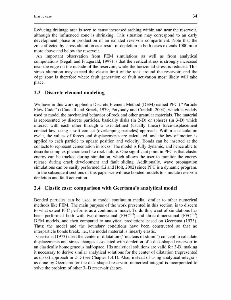
Elastic case 34 ________________________________________________________________________
Reducing drainage area is seen to cause increased arching within and near the reservoir, although the influenced zone is shrinking. This situation may correspond to an early development phase or production of an isolated reservoir compartment. Note that the zone affected by stress alteration as a result of depletion in both cases extends 1000 m or more above and below the reservoir. An important observation from FEM simulations as well as from analytical computations (Segall and Fitzgerald, 1998) is that the vertical stress is strongly increased near the edge on the outside of the reservoir, while the horizontal stress is reduced. This stress alteration may exceed the elastic limit of the rock around the reservoir, and the edge zone is therefore where fault generation or fault activation most likely will take place.
2.3 Discrete element modeling We have in this work applied a Discrete Element Method (DEM) named PFC (‘‘Particle Flow Code’’) (Cundall and Strack, 1979; Potyondy and Cundall, 2004), which is widely used to model the mechanical behavior of rock and other granular materials. The material is represented by discrete particles, basically disks (in 2-D) or spheres (in 3-D) which interact with each other through a user-defined (usually linear) force-displacement contact law, using a soft contact (overlapping particles) approach. Within a calculation cycle, the values of forces and displacements are calculated, and the law of motion is applied to each particle to update position and velocity. Bonds can be inserted at the contacts to represent cementation in rocks. The model is fully dynamic, and hence able to describe complex phenomena like rock failure. One significant point in PFC is that elastic energy can be tracked during simulation, which allows the user to monitor the energy release during crack development and fault sliding. Additionally, wave propagation simulations can be easily performed (Li and Holt, 2002) since PFC is a dynamic program. In the subsequent sections of this paper we will use bonded models to simulate reservoir depletion and fault activation.
2.4 Elastic case: comparison with Geertsma’s analytical model Bonded particles can be used to model continuum media, similar to other numerical methods like FEM. The main purpose of the work presented in this section, is to discern to what extent PFC performs as a continuum model. To do this, a set of simulations has been performed both with two-dimensional (PFC2-D) and three-dimensional (PFC3-D) DEM models, and then compared to analytical predictions based on Geertsma (1973). Thus; the model and the boundary conditions have been constructed so that no interparticle bonds break, i.e., the model material is linearly elastic. Geertsma (1973) used the center of dilatation (‘‘nucleus of strain’’) concept to calculate displacements and stress changes associated with depletion of a disk-shaped reservoir in an elastically homogeneous half-space. His analytical solutions are valid for 3-D, making it necessary to derive similar analytical solutions for the center of dilatation (represented as disks) approach in 2-D (see Chapter 1.4.1). Also, instead of using analytical integrals as done by Geertsma for the disk-shaped reservoir, numerical integral is incorporated to solve the problem of other 3- D reservoir shapes.
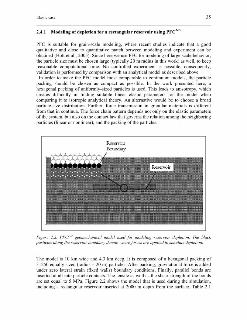
Elastic case 35 ________________________________________________________________________
2.4.1 Modeling of depletion for a rectangular reservoir using PFC2-D
PFC is suitable for grain-scale modeling, where recent studies indicate that a good qualitative and close to quantitative match between modeling and experiment can be obtained (Holt et al., 2005). Since here we use PFC for modeling of large scale behavior, the particle size must be chosen large (typically 20 m radius in this work) as well, to keep reasonable computational time. No controlled experiment is possible, consequently, validation is performed by comparison with an analytical model as described above. In order to make the PFC model most comparable to continuum models, the particle packing should be chosen as compact as possible. In the work presented here, a hexagonal packing of uniformly-sized particles is used. This leads to anisotropy, which creates difficulty in finding suitable linear elastic parameters for the model when comparing it to isotropic analytical theory. An alternative would be to choose a broad particle-size distribution. Further, force transmission in granular materials is different from that in continua. The force chain pattern depends not only on the elastic parameters of the system, but also on the contact law that governs the relation among the neighboring particles (linear or nonlinear), and the packing of the particles.
Figure 2.2. PFC2-D geomechanical model used for modeling reservoir depletion. The black particles along the reservoir boundary denote where forces are applied to simulate depletion. The model is 10 km wide and 4.3 km deep. It is composed of a hexagonal packing of 31250 equally sized (radius = 20 m) particles. After packing, gravitational force is added under zero lateral strain (fixed walls) boundary conditions. Finally, parallel bonds are inserted at all interparticle contacts. The tensile as well as the shear strength of the bonds are set equal to 5 MPa. Figure 2.2 shows the model that is used during the simulation, including a rectangular reservoir inserted at 2000 m depth from the surface. Table 2.1
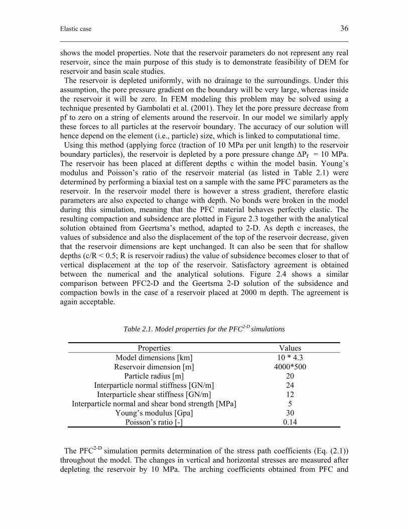
Elastic case 36 ________________________________________________________________________
shows the model properties. Note that the reservoir parameters do not represent any real reservoir, since the main purpose of this study is to demonstrate feasibility of DEM for reservoir and basin scale studies. The reservoir is depleted uniformly, with no drainage to the surroundings. Under this assumption, the pore pressure gradient on the boundary will be very large, whereas inside the reservoir it will be zero. In FEM modeling this problem may be solved using a technique presented by Gambolati et al. (2001). They let the pore pressure decrease from pf to zero on a string of elements around the reservoir. In our model we similarly apply these forces to all particles at the reservoir boundary. The accuracy of our solution will hence depend on the element (i.e., particle) size, which is linked to computational time. Using this method (applying force (traction of 10 MPa per unit length) to the reservoir boundary particles), the reservoir is depleted by a pore pressure change ΔPf = 10 MPa. The reservoir has been placed at different depths c within the model basin. Young’s modulus and Poisson’s ratio of the reservoir material (as listed in Table 2.1) were determined by performing a biaxial test on a sample with the same PFC parameters as the reservoir. In the reservoir model there is however a stress gradient, therefore elastic parameters are also expected to change with depth. No bonds were broken in the model during this simulation, meaning that the PFC material behaves perfectly elastic. The resulting compaction and subsidence are plotted in Figure 2.3 together with the analytical solution obtained from Geertsma’s method, adapted to 2-D. As depth c increases, the values of subsidence and also the displacement of the top of the reservoir decrease, given that the reservoir dimensions are kept unchanged. It can also be seen that for shallow depths (c/R < 0.5; R is reservoir radius) the value of subsidence becomes closer to that of vertical displacement at the top of the reservoir. Satisfactory agreement is obtained between the numerical and the analytical solutions. Figure 2.4 shows a similar comparison between PFC2-D and the Geertsma 2-D solution of the subsidence and compaction bowls in the case of a reservoir placed at 2000 m depth. The agreement is again acceptable.
Table 2.1. Model properties for the PFC2-D simulations
Properties Values Model dimensions [km] 10 * 4.3 Reservoir dimension [m] 4000*500
Particle radius [m] 20 Interparticle normal stiffness [GN/m] 24 Interparticle shear stiffness [GN/m] 12
Interparticle normal and shear bond strength [MPa] 5 Young’s modulus [Gpa] 30
Poisson’s ratio [-] 0.14 The PFC2-D simulation permits determination of the stress path coefficients (Eq. (2.1)) throughout the model. The changes in vertical and horizontal stresses are measured after depleting the reservoir by 10 MPa. The arching coefficients obtained from PFC and
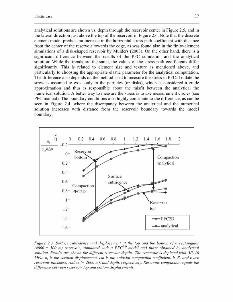
Elastic case 37 ________________________________________________________________________
analytical solutions are shown vs. depth through the reservoir center in Figure 2.5, and in the lateral direction just above the top of the reservoir in Figure 2.6. Note that the discrete element model predicts an increase in the horizontal stress path coefficient with distance from the center of the reservoir towards the edge, as was found also in the finite-element simulations of a disk-shaped reservoir by Mulders (2003). On the other hand, there is a significant difference between the results of the PFC simulation and the analytical solution: While the trends are the same, the values of the stress path coefficients differ significantly. This is related to element size and texture as mentioned above, and particularly to choosing the appropriate elastic parameter for the analytical computation. The difference also depends on the method used to measure the stress in PFC: To date the stress is assumed to exist only in the particles (or disks), which is considered a crude approximation and thus is responsible about the misfit between the analytical the numerical solution. A better way to measure the stress is to use measurement circles (see PFC manual). The boundary conditions also highly contribute to the difference, as can be seen in Figure 2.4, where the discrepancy between the analytical and the numerical solution increases with distance from the reservoir boundary towards the model boundary.
Figure 2.3. Surface subsidence and displacement at the top and the bottom of a rectangular (4000 * 500 m) reservoir, simulated with a PFC2-D model and those obtained by analytical solution. Results are shown for different reservoir depths. The reservoir is depleted with ΔPf 10 MPa. uz is the vertical displacement, cm is the uniaxial compaction coefficient, h, R, and c are reservoir thickness, radius (= 2000 m), and depth, respectively. Reservoir compaction equals the difference between reservoir top and bottom displacements.
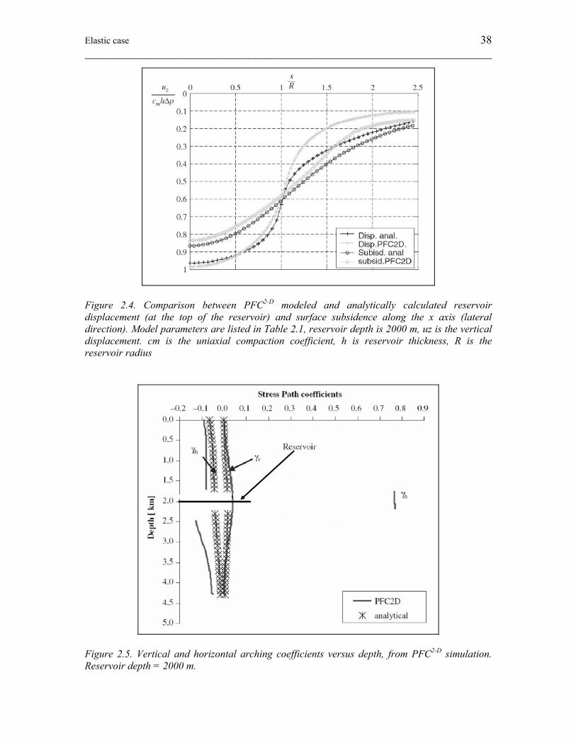
Elastic case 38 ________________________________________________________________________
Figure 2.4. Comparison between PFC2-D modeled and analytically calculated reservoir displacement (at the top of the reservoir) and surface subsidence along the x axis (lateral direction). Model parameters are listed in Table 2.1, reservoir depth is 2000 m, uz is the vertical displacement. cm is the uniaxial compaction coefficient, h is reservoir thickness, R is the reservoir radius
Figure 2.5. Vertical and horizontal arching coefficients versus depth, from PFC2-D simulation. Reservoir depth = 2000 m.
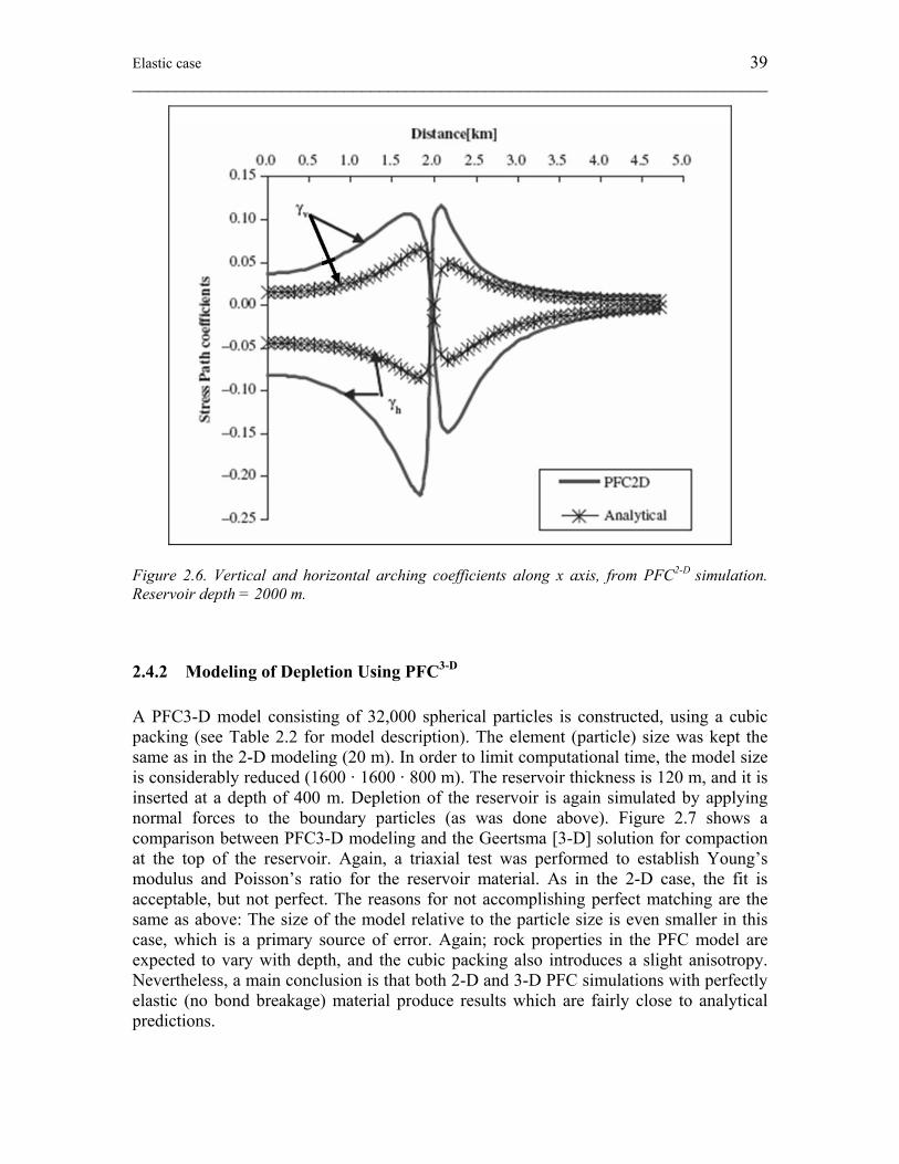
Elastic case 39 ________________________________________________________________________
Figure 2.6. Vertical and horizontal arching coefficients along x axis, from PFC2-D simulation. Reservoir depth = 2000 m.
2.4.2 Modeling of Depletion Using PFC3-D A PFC3-D model consisting of 32,000 spherical particles is constructed, using a cubic packing (see Table 2.2 for model description). The element (particle) size was kept the same as in the 2-D modeling (20 m). In order to limit computational time, the model size is considerably reduced (1600 · 1600 · 800 m). The reservoir thickness is 120 m, and it is inserted at a depth of 400 m. Depletion of the reservoir is again simulated by applying normal forces to the boundary particles (as was done above). Figure 2.7 shows a comparison between PFC3-D modeling and the Geertsma [3-D] solution for compaction at the top of the reservoir. Again, a triaxial test was performed to establish Young’s modulus and Poisson’s ratio for the reservoir material. As in the 2-D case, the fit is acceptable, but not perfect. The reasons for not accomplishing perfect matching are the same as above: The size of the model relative to the particle size is even smaller in this case, which is a primary source of error. Again; rock properties in the PFC model are expected to vary with depth, and the cubic packing also introduces a slight anisotropy. Nevertheless, a main conclusion is that both 2-D and 3-D PFC simulations with perfectly elastic (no bond breakage) material produce results which are fairly close to analytical predictions.
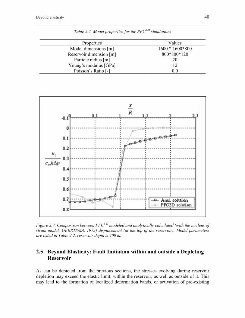
Beyond elasticity 40 ________________________________________________________________________
Table 2.2. Model properties for the PFC3-D simulations
Properties Values Model dimensions [m] 1600 * 1600*800
Reservoir dimension [m] 800*800*120 Particle radius [m] 20
Young’s modulus [GPa] 12 Poisson’s Ratio [-] 0.0
Figure 2.7. Comparison between PFC3-D modeled and analytically calculated (with the nucleus of strain model; GEERTSMA, 1973) displacement (at the top of the reservoir). Model parameters are listed in Table 2.2, reservoir depth is 400 m.
2.5 Beyond Elasticity: Fault Initiation within and outside a Depleting Reservoir
As can be depicted from the previous sections, the stresses evolving during reservoir depletion may exceed the elastic limit; within the reservoir, as well as outside of it. This may lead to the formation of localized deformation bands, or activation of pre-existing
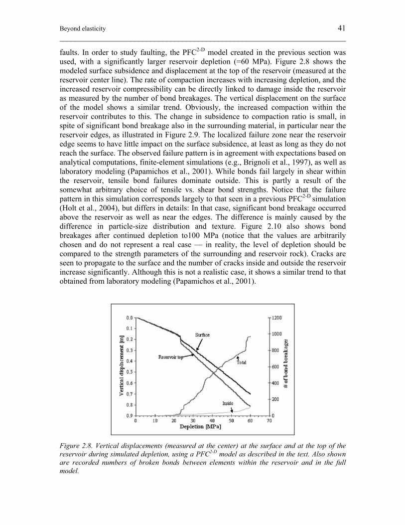
Beyond elasticity 41 ________________________________________________________________________
faults. In order to study faulting, the PFC2-D model created in the previous section was used, with a significantly larger reservoir depletion (=60 MPa). Figure 2.8 shows the modeled surface subsidence and displacement at the top of the reservoir (measured at the reservoir center line). The rate of compaction increases with increasing depletion, and the increased reservoir compressibility can be directly linked to damage inside the reservoir as measured by the number of bond breakages. The vertical displacement on the surface of the model shows a similar trend. Obviously, the increased compaction within the reservoir contributes to this. The change in subsidence to compaction ratio is small, in spite of significant bond breakage also in the surrounding material, in particular near the reservoir edges, as illustrated in Figure 2.9. The localized failure zone near the reservoir edge seems to have little impact on the surface subsidence, at least as long as they do not reach the surface. The observed failure pattern is in agreement with expectations based on analytical computations, finite-element simulations (e.g., Brignoli et al., 1997), as well as laboratory modeling (Papamichos et al., 2001). While bonds fail largely in shear within the reservoir, tensile bond failures dominate outside. This is partly a result of the somewhat arbitrary choice of tensile vs. shear bond strengths. Notice that the failure pattern in this simulation corresponds largely to that seen in a previous PFC2-D simulation (Holt et al., 2004), but differs in details: In that case, significant bond breakage occurred above the reservoir as well as near the edges. The difference is mainly caused by the difference in particle-size distribution and texture. Figure 2.10 also shows bond breakages after continued depletion to100 MPa (notice that the values are arbitrarily chosen and do not represent a real case — in reality, the level of depletion should be compared to the strength parameters of the surrounding and reservoir rock). Cracks are seen to propagate to the surface and the number of cracks inside and outside the reservoir increase significantly. Although this is not a realistic case, it shows a similar trend to that obtained from laboratory modeling (Papamichos et al., 2001).
Figure 2.8. Vertical displacements (measured at the center) at the surface and at the top of the reservoir during simulated depletion, using a PFC2-D model as described in the text. Also shown are recorded numbers of broken bonds between elements within the reservoir and in the full model.
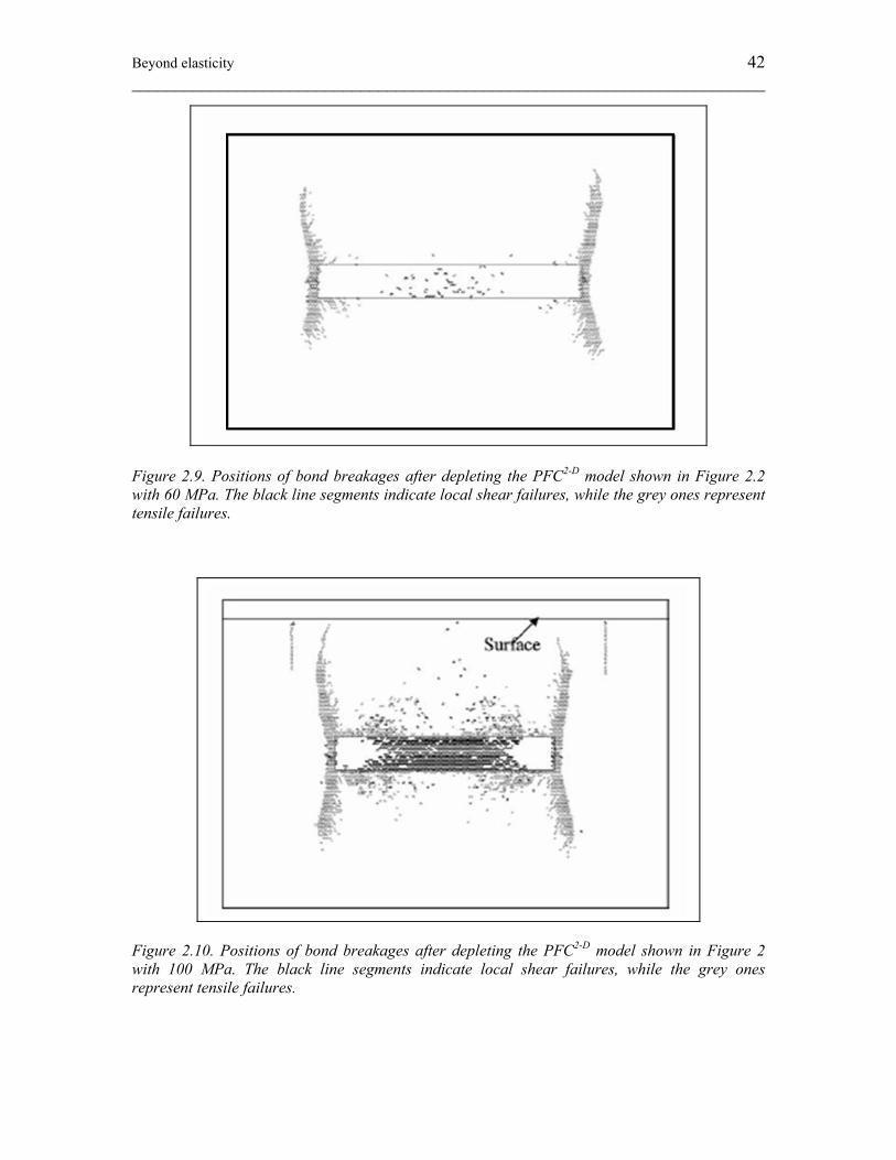
Beyond elasticity 42 ________________________________________________________________________
Figure 2.9. Positions of bond breakages after depleting the PFC2-D model shown in Figure 2.2 with 60 MPa. The black line segments indicate local shear failures, while the grey ones represent tensile failures.
Figure 2.10. Positions of bond breakages after depleting the PFC2-D model shown in Figure 2 with 100 MPa. The black line segments indicate local shear failures, while the grey ones represent tensile failures.
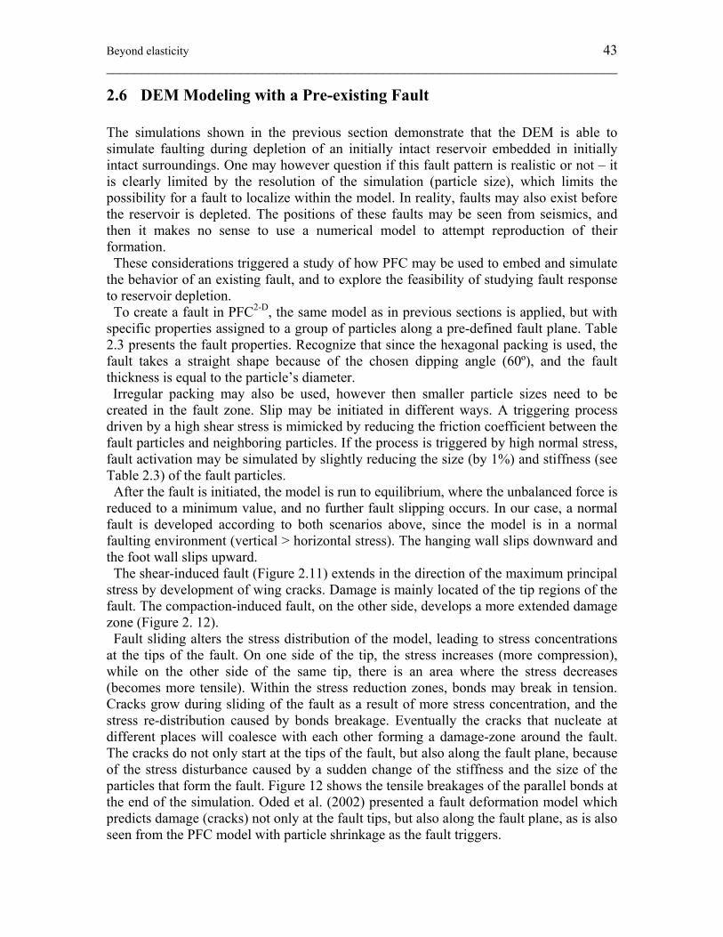
Beyond elasticity 43 ________________________________________________________________________
2.6 DEM Modeling with a Pre-existing Fault The simulations shown in the previous section demonstrate that the DEM is able to simulate faulting during depletion of an initially intact reservoir embedded in initially intact surroundings. One may however question if this fault pattern is realistic or not – it is clearly limited by the resolution of the simulation (particle size), which limits the possibility for a fault to localize within the model. In reality, faults may also exist before the reservoir is depleted. The positions of these faults may be seen from seismics, and then it makes no sense to use a numerical model to attempt reproduction of their formation. These considerations triggered a study of how PFC may be used to embed and simulate the behavior of an existing fault, and to explore the feasibility of studying fault response to reservoir depletion. To create a fault in PFC2-D, the same model as in previous sections is applied, but with specific properties assigned to a group of particles along a pre-defined fault plane. Table 2.3 presents the fault properties. Recognize that since the hexagonal packing is used, the fault takes a straight shape because of the chosen dipping angle (60º), and the fault thickness is equal to the particle’s diameter. Irregular packing may also be used, however then smaller particle sizes need to be created in the fault zone. Slip may be initiated in different ways. A triggering process driven by a high shear stress is mimicked by reducing the friction coefficient between the fault particles and neighboring particles. If the process is triggered by high normal stress, fault activation may be simulated by slightly reducing the size (by 1%) and stiffness (see Table 2.3) of the fault particles. After the fault is initiated, the model is run to equilibrium, where the unbalanced force is reduced to a minimum value, and no further fault slipping occurs. In our case, a normal fault is developed according to both scenarios above, since the model is in a normal faulting environment (vertical > horizontal stress). The hanging wall slips downward and the foot wall slips upward. The shear-induced fault (Figure 2.11) extends in the direction of the maximum principal stress by development of wing cracks. Damage is mainly located of the tip regions of the fault. The compaction-induced fault, on the other side, develops a more extended damage zone (Figure 2. 12). Fault sliding alters the stress distribution of the model, leading to stress concentrations at the tips of the fault. On one side of the tip, the stress increases (more compression), while on the other side of the same tip, there is an area where the stress decreases (becomes more tensile). Within the stress reduction zones, bonds may break in tension. Cracks grow during sliding of the fault as a result of more stress concentration, and the stress re-distribution caused by bonds breakage. Eventually the cracks that nucleate at different places will coalesce with each other forming a damage-zone around the fault. The cracks do not only start at the tips of the fault, but also along the fault plane, because of the stress disturbance caused by a sudden change of the stiffness and the size of the particles that form the fault. Figure 12 shows the tensile breakages of the parallel bonds at the end of the simulation. Oded et al. (2002) presented a fault deformation model which predicts damage (cracks) not only at the fault tips, but also along the fault plane, as is also seen from the PFC model with particle shrinkage as the fault triggers.
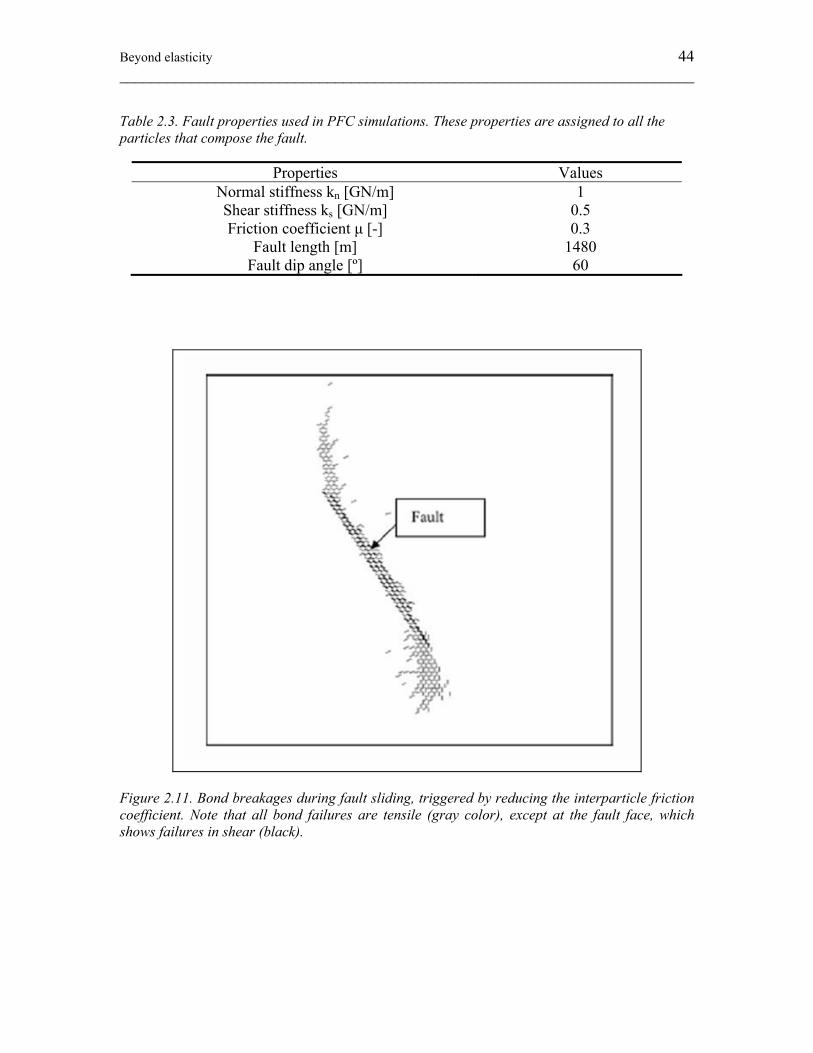
Beyond elasticity 44 ________________________________________________________________________
Table 2.3. Fault properties used in PFC simulations. These properties are assigned to all the particles that compose the fault.
Properties Values Normal stiffness kn [GN/m] 1 Shear stiffness ks [GN/m] 0.5 Friction coefficient μ [-] 0.3
Fault length [m] 1480 Fault dip angle [º] 60
Figure 2.11. Bond breakages during fault sliding, triggered by reducing the interparticle friction coefficient. Note that all bond failures are tensile (gray color), except at the fault face, which shows failures in shear (black).
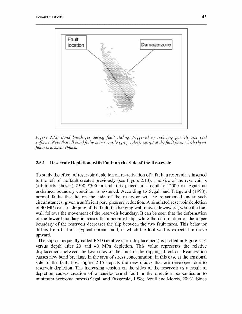
Beyond elasticity 45 ________________________________________________________________________
Figure 2.12. Bond breakages during fault sliding, triggered by reducing particle size and stiffness. Note that all bond failures are tensile (gray color), except at the fault face, which shows failures in shear (black).
2.6.1 Reservoir Depletion, with Fault on the Side of the Reservoir To study the effect of reservoir depletion on re-activation of a fault, a reservoir is inserted to the left of the fault created previously (see Figure 2.13). The size of the reservoir is (arbitrarily chosen) 2500 *500 m and it is placed at a depth of 2000 m. Again an undrained boundary condition is assumed. According to Segall and Fitzgerald (1998), normal faults that lie on the side of the reservoir will be re-activated under such circumstances, given a sufficient pore pressure reduction. A simulated reservoir depletion of 40 MPa causes slipping of the fault, the hanging wall moves downward, while the foot wall follows the movement of the reservoir boundary. It can be seen that the deformation of the lower boundary increases the amount of slip, while the deformation of the upper boundary of the reservoir decreases the slip between the two fault faces. This behavior differs from that of a typical normal fault, in which the foot wall is expected to move upward. The slip or frequently called RSD (relative shear displacement) is plotted in Figure 2.14 versus depth after 20 and 40 MPa depletion. This value represents the relative displacement between the two sides of the fault in the dipping direction. Reactivation causes new bond breakage in the area of stress concentration; in this case at the tensional side of the fault tips. Figure 2.15 depicts the new cracks that are developed due to reservoir depletion. The increasing tension on the sides of the reservoir as a result of depletion causes creation of a tensile-normal fault in the direction perpendicular to minimum horizontal stress (Segall and Fitzgerald, 1998; Ferrill and Morris, 2003). Since
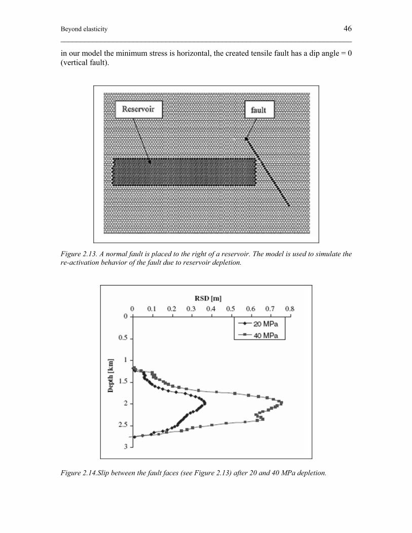
Beyond elasticity 46 ________________________________________________________________________
in our model the minimum stress is horizontal, the created tensile fault has a dip angle = 0 (vertical fault).
Figure 2.13. A normal fault is placed to the right of a reservoir. The model is used to simulate the re-activation behavior of the fault due to reservoir depletion.
Figure 2.14.Slip between the fault faces (see Figure 2.13) after 20 and 40 MPa depletion.
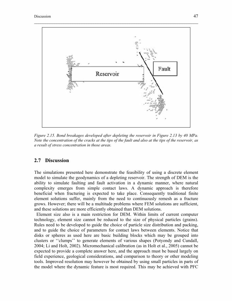
Discussion 47 ________________________________________________________________________
Figure 2.15. Bond breakages developed after depleting the reservoir in Figure 2.13 by 40 MPa. Note the concentration of the cracks at the tips of the fault and also at the tips of the reservoir, as a result of stress concentration in those areas.
2.7 Discussion The simulations presented here demonstrate the feasibility of using a discrete element model to simulate the geodynamics of a depleting reservoir. The strength of DEM is the ability to simulate faulting and fault activation in a dynamic manner, where natural complexity emerges from simple contact laws. A dynamic approach is therefore beneficial when fracturing is expected to take place. Consequently traditional finite element solutions suffer, mainly from the need to continuously remesh as a fracture grows. However; there will be a multitude problems where FEM solutions are sufficient, and these solutions are more efficiently obtained than DEM solutions. Element size also is a main restriction for DEM. Within limits of current computer technology, element size cannot be reduced to the size of physical particles (grains). Rules need to be developed to guide the choice of particle size distribution and packing, and to guide the choice of parameters for contact laws between elements. Notice that disks or spheres as used here are basic building blocks which may be grouped into clusters or ‘‘clumps’’ to generate elements of various shapes (Potyondy and Cundall, 2004; Li and Holt, 2002). Micromechanical calibration (as in Holt et al., 2005) cannot be expected to provide a complete answer here, and the approach must be based largely on field experience, geological considerations, and comparison to theory or other modeling tools. Improved resolution may however be obtained by using small particles in parts of the model where the dynamic feature is most required. This may be achieved with PFC
Discussion 48 ________________________________________________________________________
by utilizing a recent option (AC/DC) for automatic linkage of the DEM to a continuum (e.g., FEM or finite difference) model. In the PFC simulations shown here, poromechanical coupling was (for simplicity) not applied. This is however possible (Shimizu, 2004; Li and Holt, 2004), and would permit more realistic treatments of pressure gradients within a reservoir compartment and across faults. This also permits well drainage to be part of the model. Currently, only single phase fluid flow has been coupled to PFC, nonetheless this is not a fundamental limitation. Also, since wave propagation can be performed relatively easy with PFC (Li and Holt, 2002), direct simulations of seismic surveys as well as induced seismicity (Hazzard and Young, 2000) may be incorporated within the same scheme as the geomechanical and fluid flow simulations.
2.8 Conclusions We have demonstrated the feasibility of a Discrete Element Model (PFC) to simulate stress evolution and associated displacements resulting from pore pressure depletion of a producing reservoir. The model was calibrated in 2-D as well as 3-D for a case of perfect elasticity, when comparison could be made to analytical calculations by the nucleus of strain theory (Geertsma, 1973). The accuracy of the DEM is limited by element size, which here was 20 m (given by the radius of disk elements in 2-D; spheres in 3-D). While calculated compaction and subsidence were in good agreement with theory, the scatter in stress calculations was more significant. The results are also sensitive to particle sizedistribution and packing, indicating that more work is required to optimize the choices of these parameters and parameters controlling the contact law between particles. Also as with other numerical methods, the results are largely affected by the boundary conditions. Therefore the model must be refined to achieve better results. The simulations performed illustrate the ability of the DEM to generate localized faults when the elastic limit is exceeded somewhere in the model. As one would expect from analytical stress calculations and from previous numerical work, faulting is likely to take place in the surrounding near the edge of a depleting reservoir. When faults are known to exist prior to depletion and can be identified from seismic images, they may be embedded in the DEM model by selecting an array of particles with properties different from the surroundings. In our case, two options for numerical simulation of fault activation were considered; (i) reduced friction; (ii) reduced particle size and stiffness. Further work is required to find a geologically representative formulation for a fault in the DEM. We conclude that DEM, such as PFC, may provide useful insight into the dynamic behavior of a rock mass such as in the case of a depleting reservoir embedded in a sedimentary basin. In principle, fluid flow and elastic wave propagation may also be incorporated in this model. Only when faulting is expected to take place will DEM be beneficial compared to more traditional simulation approaches (like FEM). Improvements include reducing particle (element) size, particularly in zones where failure may occur. Linking of DEM to a continuum model appears to be a promising tool.
Chapter 3: Relating DEM parameters to rock properties 49 ________________________________________________________________________
3 Relating discrete element method (DEM) parameters to rock properties
*Part of this chapter is presented and published at the proceeding of FLAC/DEM Symposium, Minneapolis, USA, 2008. Another part is presented at EAGE conference, Vienna, 2006, and appeared in the Extended Abstract.
3.1 Introduction In Chapter 2 a feasibility study is presented to show the possibility of using DEM in large scale reservoir geomechanics. The study is conducted without looking into much detail about how to relate DEM parameters to conventional rock properties. For example, to obtain the values of the Young’s modulus E and the Poisson’s ratio ν, a biaxial test on a sample that resembles the geomechanical model material is performed. However, if we want to use DEM as a general method in reservoir geomechanics, general and concrete relations must be derived to relate DEM Parameters like kn, ks to rock properties like E and ν. In this chapter we will use an approach based on Walton’s model for granular media (1987) to derive such relations. In the first section, the Walton approach is revisited and used to derive a relatively general formula for the elastic constitutive relation Cijkl, the formula uses DEM parameters kn, ks for the contact normal and shear stiffness instead of the Hertz-Mindlin contact law used by Walton. Then, this formula is used to derive relations for dense packing of two types, hexagonal and square. A modification for the square packing is done to guarantee isotropic behavior. These relations are tested by dynamic and static tests, such as wave propagation in both homogeneous and heterogeneous media, also biaxial and reservoir geomechanical tests. After that, relations for a loose, dense packing are derived, and a technique is presented to show how many particles are needed to give isotropic packing. It is also shown that the dynamic behavior for the loose packing is different from the static one. For example, based on two dimensional simulation it is found that the dynamic Poisson’s ratio is limited to 0.25 (based on plane-strain condition) i.e. the maximum P-/S-wave velocity ratio is limited by Vp/Vs < 3 . The static Poisson’s ratio is however not limited by the same value. Empirical relations for the static behavior are derived based on observing numerical tests and some dimensional analysis. Next, a procedure for creating a failure envelope for DEM models is presented. The procedure relies on numerical simulations of Biaxial and Brazilian tests to extract the failure properties. Since until now we could not obtain failure relations for DEM similar to the elastic relations, one may use such a procedure to get the failure properties for the DEM models. Then, we show how one may construct a velocity model from a DEM geomechanical model to be used later in seismic modeling. In the last section, we study the effect of particle rotation on the elastic properties using Cosserat continuum theory.
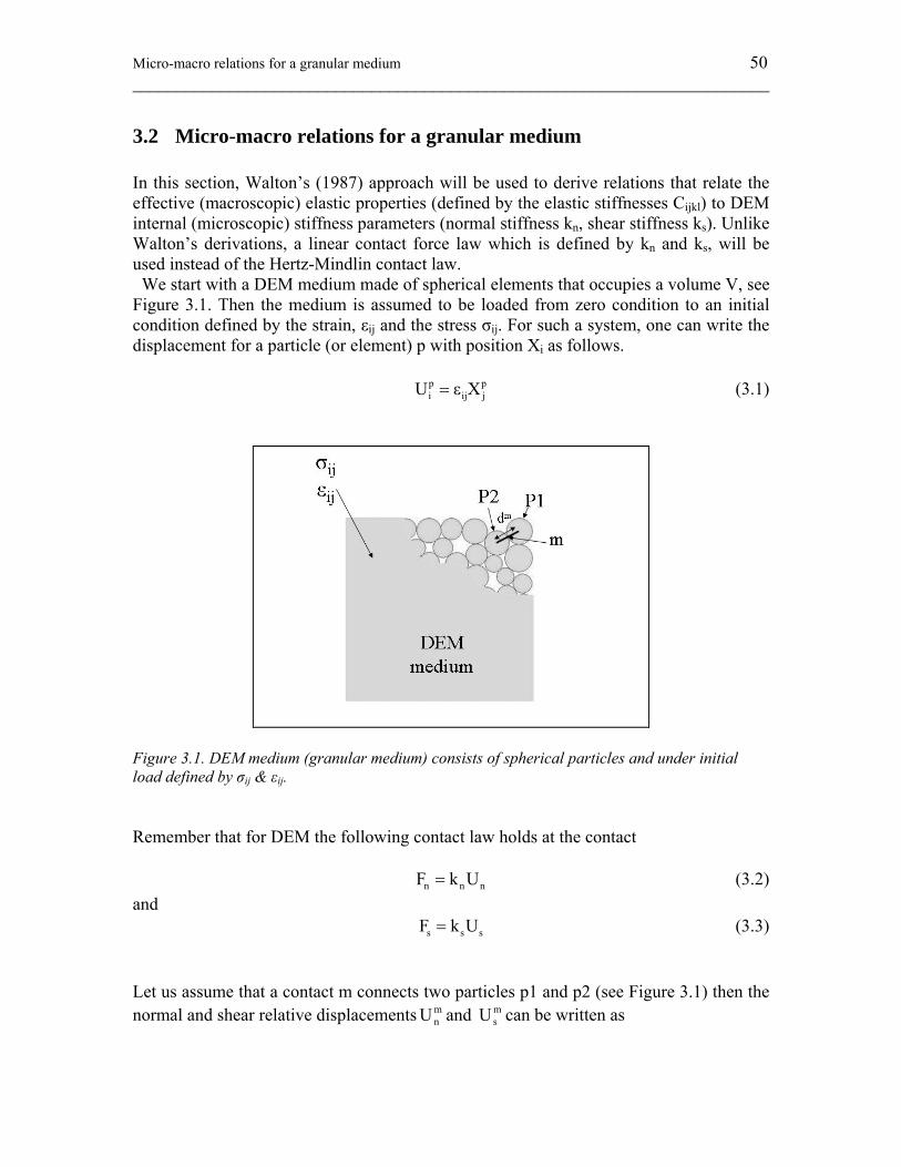
Micro-macro relations for a granular medium 50 ________________________________________________________________________
3.2 Micro-macro relations for a granular medium In this section, Walton’s (1987) approach will be used to derive relations that relate the effective (macroscopic) elastic properties (defined by the elastic stiffnesses Cijkl) to DEM internal (microscopic) stiffness parameters (normal stiffness kn, shear stiffness ks). Unlike Walton’s derivations, a linear contact force law which is defined by kn and ks, will be used instead of the Hertz-Mindlin contact law. We start with a DEM medium made of spherical elements that occupies a volume V, see Figure 3.1. Then the medium is assumed to be loaded from zero condition to an initial condition defined by the strain, εij and the stress σij. For such a system, one can write the displacement for a particle (or element) p with position Xi as follows. p p
i ij jU ε X= (3.1)
Figure 3.1. DEM medium (granular medium) consists of spherical particles and under initial load defined by σij & εij. Remember that for DEM the following contact law holds at the contact n n nF k U= (3.2) and s s sF k U= (3.3) Let us assume that a contact m connects two particles p1 and p2 (see Figure 3.1) then the normal and shear relative displacements m
nU and msU can be written as
Micro-macro relations for a granular medium 51 ________________________________________________________________________
m m mn i iU ΔU I= (3.4)
and m m m m
s(i) i n iU ΔU U I= − (3.5) where the relative displacement at the contact m
iUΔ is given as, m p1 p2
i ij j jΔU ε (X X )= − (3.6) The normal unit vector m
iI is given as
p1 p2
m i ii
m
X XId−
= (3.7)
dm is the contact length, i.e. distance between p1 and p2. The total force Fi at contact m can be written as m m m m m m m m m m
i n j j i s i j j iF k ΔU I I k (ΔU ΔU I I )= + − (3.8) or m m m m m m m m
i n s kl k l i m s ij j mF (k - k )(ε I I )I d k ε I d= + (3.9) Notice that summation Einstein convention with dummy subscript i,j,k,l is used in the above equations. Further more, by using Cauchy’s formula (see Walton, 1987), the average stress σij can be written as
c cij i j j i
S
1σ (X T X T ) S2V
= + ∂∫ (3.10)
where S represents the spheres’ surface, c
iX is the distance between a contact on the surface of a sphere and its center, and Ti is the surface traction. Since we have discrete element medium with distinct contacts being assumed as points, the integral in Eq. (3.10) can be replaced by summation. Besides, instead of summing over the spheres while measuring the stress we sum over the contacts. So Eq. (3.10) may be written as
Nc
m m m mij m i j m j i
m 1
1σ (d I F d I F )2V =
= +∑ (3.11)
Nc is the number of contacts inside the medium. Notice that since m c
m i id I 2X= , another factor ½ should appear in Eq. (3.11). However since we are summing over the contacts instead of the spheres, each contact is counted once. This is opposite to the case in Eq. (3.10) where each contact is counted twice. Now, by substituting Eq. (3.9) into Eq. (3.11), we end up with
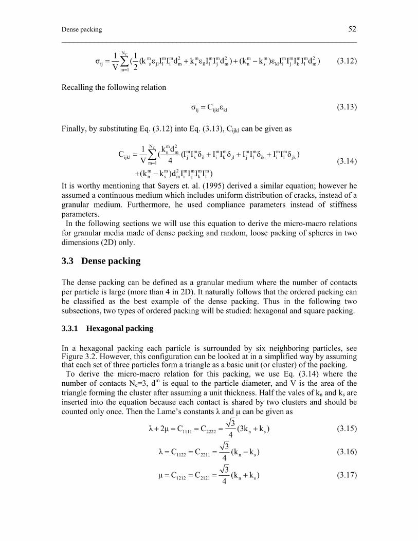
Dense packing 52 ________________________________________________________________________
CN
m m m 2 m m m 2 m m m m m m 2ij s jl l i m s il l j m n s kl i j k l m
m 1
1 1σ ( (k ε I I d k ε I I d ) (k k )ε I I I I d )V 2=
= + + −∑ (3.12)
Recalling the following relation ij ijkl klσ C ε= (3.13) Finally, by substituting Eq. (3.12) into Eq. (3.13), Cijkl can be given as
CN m 2m m m m m m m ms m
ijkl j k il i k jl j l ik i l jkm 1m m 2 m m m mn s m i j k l
k d1C ( (I I δ I I δ I I δ I I δ )V 4(k k )d I I I I )
=
= + + +
+ −
∑ (3.14)
It is worthy mentioning that Sayers et. al. (1995) derived a similar equation; however he assumed a continuous medium which includes uniform distribution of cracks, instead of a granular medium. Furthermore, he used compliance parameters instead of stiffness parameters. In the following sections we will use this equation to derive the micro-macro relations for granular media made of dense packing and random, loose packing of spheres in two dimensions (2D) only.
3.3 Dense packing The dense packing can be defined as a granular medium where the number of contacts per particle is large (more than 4 in 2D). It naturally follows that the ordered packing can be classified as the best example of the dense packing. Thus in the following two subsections, two types of ordered packing will be studied: hexagonal and square packing.
3.3.1 Hexagonal packing In a hexagonal packing each particle is surrounded by six neighboring particles, see Figure 3.2. However, this configuration can be looked at in a simplified way by assuming that each set of three particles form a triangle as a basic unit (or cluster) of the packing. To derive the micro-macro relation for this packing, we use Eq. (3.14) where the number of contacts Nc=3, dm is equal to the particle diameter, and V is the area of the triangle forming the cluster after assuming a unit thickness. Half the vales of kn and ks are inserted into the equation because each contact is shared by two clusters and should be counted only once. Then the Lame’s constants λ and μ can be given as
1111 2222 n s3λ 2μ C C (3k k )
4+ = = = + (3.15)
1122 2211 n s3λ C C (k k )
4= = = − (3.16)
1212 2121 n s3μ C C (k k )
4= = = + (3.17)
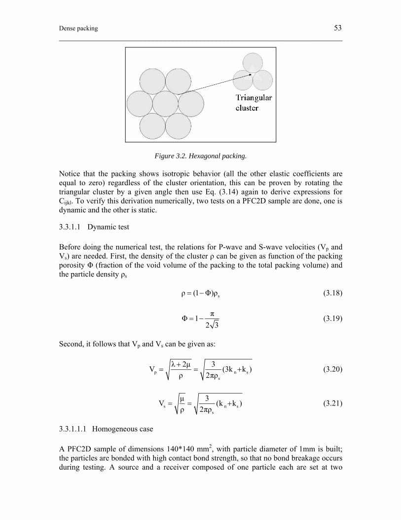
Dense packing 53 ________________________________________________________________________
Figure 3.2. Hexagonal packing. Notice that the packing shows isotropic behavior (all the other elastic coefficients are equal to zero) regardless of the cluster orientation, this can be proven by rotating the triangular cluster by a given angle then use Eq. (3.14) again to derive expressions for Cijkl. To verify this derivation numerically, two tests on a PFC2D sample are done, one is dynamic and the other is static.
3.3.1.1 Dynamic test Before doing the numerical test, the relations for P-wave and S-wave velocities (Vp and Vs) are needed. First, the density of the cluster ρ can be given as function of the packing porosity Φ (fraction of the void volume of the packing to the total packing volume) and the particle density ρs sρ (1 Φ)ρ= − (3.18)
πΦ 12 3
= − (3.19)
Second, it follows that Vp and Vs can be given as:
p n ss
λ 2μ 3V (3k k )ρ 2πρ+
= = + (3.20)
s n ss
μ 3V (k k )ρ 2πρ
= = + (3.21)
3.3.1.1.1 Homogeneous case A PFC2D sample of dimensions 140*140 mm2, with particle diameter of 1mm is built; the particles are bonded with high contact bond strength, so that no bond breakage occurs during testing. A source and a receiver composed of one particle each are set at two
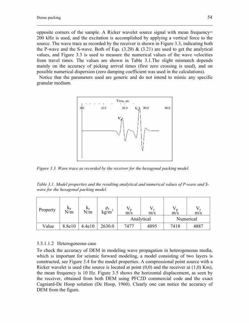
Dense packing 54 ________________________________________________________________________
opposite corners of the sample. A Ricker wavelet source signal with mean frequency= 200 kHz is used, and the excitation is accomplished by applying a vertical force to the source. The wave trace as recorded by the receiver is shown in Figure 3.3, indicating both the P-wave and the S-wave. Both of Eqs. (3.20) & (3.21) are used to get the analytical values, and Figure 3.3 is used to measure the numerical values of the wave velocities from travel times. The values are shown in Table 3.1.The slight mismatch depends mainly on the accuracy of picking arrival times (first zero crossing is used), and on possible numerical dispersion (zero damping coefficient was used in the calculations). Notice that the parameters used are generic and do not intend to mimic any specific granular medium.
Figure 3.3. Wave trace as recorded by the receiver for the hexagonal packing model. Table 3.1. Model properties and the resulting analytical and numerical values of P-wave and S-wave for the hexagonal packing model.
Vp m/s
Vs m/s
Vp m/s
Vs m/s Property kn
N/m ks
N/m ρs
kg/m3 Analytical Numerical
Value 8.8e10 4.4e10 2630.0 7477 4895 7418 4887
3.3.1.1.2 Heterogeneous case To check the accuracy of DEM in modeling wave propagation in heterogeneous media, which is important for seismic forward modeling, a model consisting of two layers is constructed, see Figure 3.4 for the model properties. A compressional point source with a Ricker wavelet is used (the source is located at point (0,0) and the receiver at (1,0) Km), the mean frequency is 10 Hz. Figure 3.5 shows the horizontal displacement, as seen by the receiver, obtained from both DEM using PFC2D commercial code and the exact Cagniard-De Hoop solution (De Hoop, 1960). Clearly one can notice the accuracy of DEM from the figure.
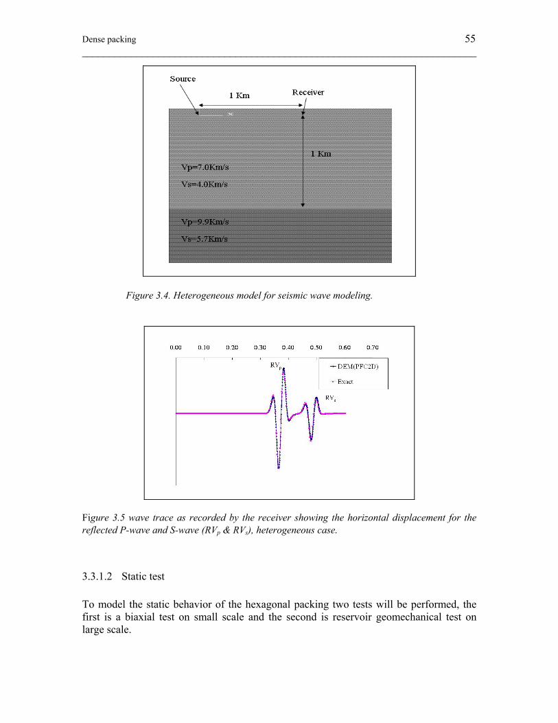
Dense packing 55 ________________________________________________________________________
Figure 3.4. Heterogeneous model for seismic wave modeling.
Figure 3.5 wave trace as recorded by the receiver showing the horizontal displacement for the reflected P-wave and S-wave (RVp & RVs), heterogeneous case.
3.3.1.2 Static test To model the static behavior of the hexagonal packing two tests will be performed, the first is a biaxial test on small scale and the second is reservoir geomechanical test on large scale.
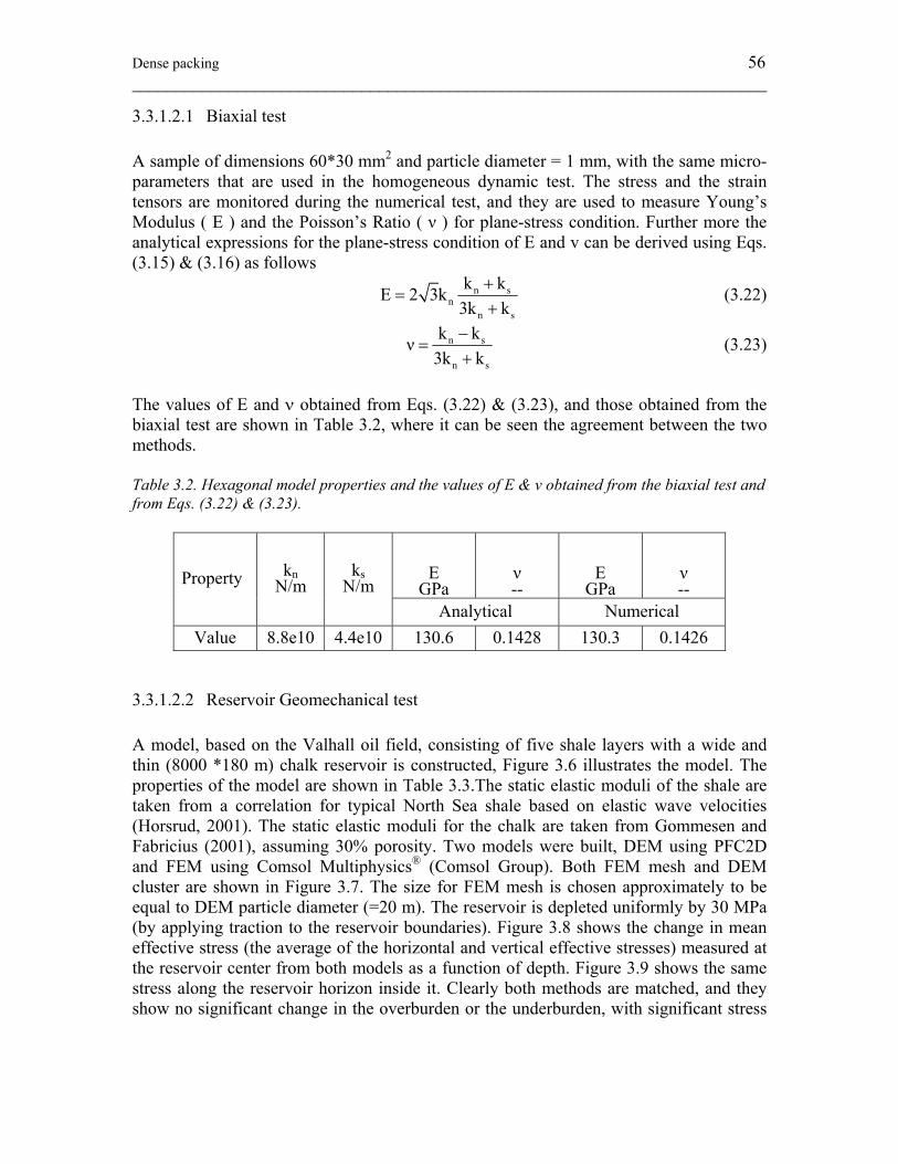
Dense packing 56 ________________________________________________________________________
3.3.1.2.1 Biaxial test A sample of dimensions 60*30 mm2 and particle diameter = 1 mm, with the same micro-parameters that are used in the homogeneous dynamic test. The stress and the strain tensors are monitored during the numerical test, and they are used to measure Young’s Modulus ( E ) and the Poisson’s Ratio ( ν ) for plane-stress condition. Further more the analytical expressions for the plane-stress condition of E and v can be derived using Eqs. (3.15) & (3.16) as follows
n sn
n s
k kE 2 3k3k k
+=
+ (3.22)
n s
n s
k kν3k k
−=
+ (3.23)
The values of E and ν obtained from Eqs. (3.22) & (3.23), and those obtained from the biaxial test are shown in Table 3.2, where it can be seen the agreement between the two methods. Table 3.2. Hexagonal model properties and the values of E & ν obtained from the biaxial test and from Eqs. (3.22) & (3.23).
E GPa
ν --
E GPa
ν -- Property kn
N/m ks
N/m Analytical Numerical
Value 8.8e10 4.4e10 130.6 0.1428 130.3 0.1426
3.3.1.2.2 Reservoir Geomechanical test A model, based on the Valhall oil field, consisting of five shale layers with a wide and thin (8000 *180 m) chalk reservoir is constructed, Figure 3.6 illustrates the model. The properties of the model are shown in Table 3.3.The static elastic moduli of the shale are taken from a correlation for typical North Sea shale based on elastic wave velocities (Horsrud, 2001). The static elastic moduli for the chalk are taken from Gommesen and Fabricius (2001), assuming 30% porosity. Two models were built, DEM using PFC2D and FEM using Comsol Multiphysics® (Comsol Group). Both FEM mesh and DEM cluster are shown in Figure 3.7. The size for FEM mesh is chosen approximately to be equal to DEM particle diameter (=20 m). The reservoir is depleted uniformly by 30 MPa (by applying traction to the reservoir boundaries). Figure 3.8 shows the change in mean effective stress (the average of the horizontal and vertical effective stresses) measured at the reservoir center from both models as a function of depth. Figure 3.9 shows the same stress along the reservoir horizon inside it. Clearly both methods are matched, and they show no significant change in the overburden or the underburden, with significant stress
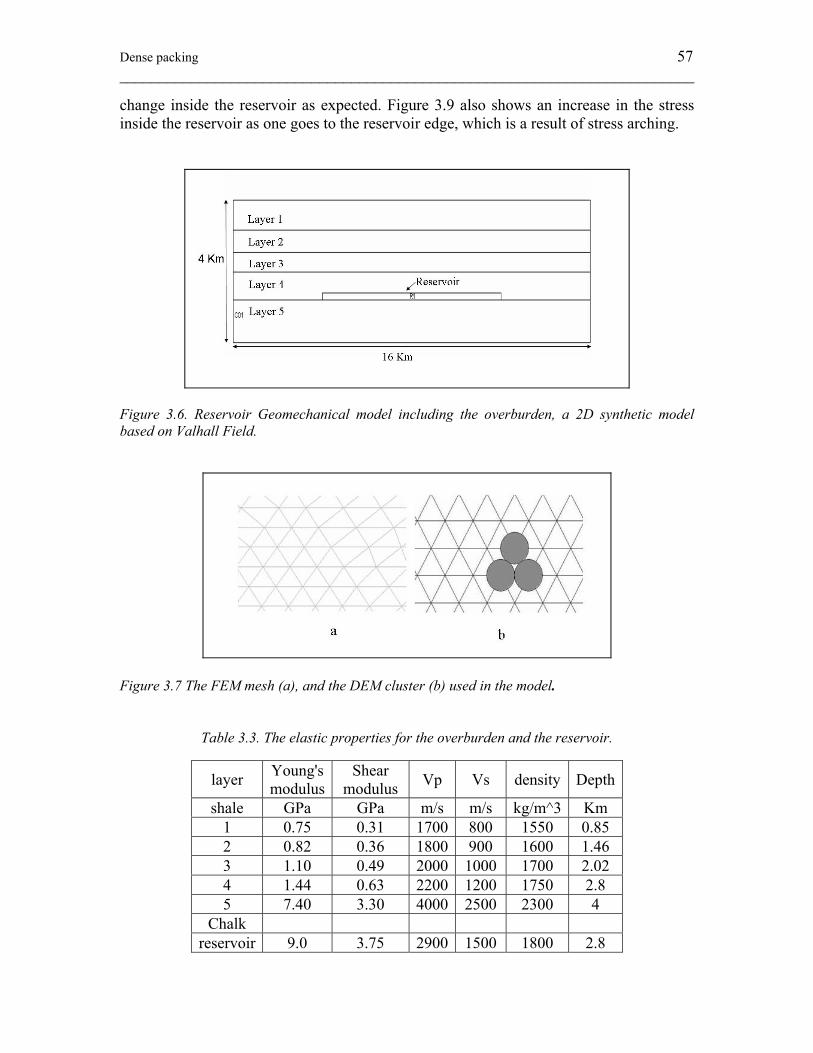
Dense packing 57 ________________________________________________________________________
change inside the reservoir as expected. Figure 3.9 also shows an increase in the stress inside the reservoir as one goes to the reservoir edge, which is a result of stress arching.
Figure 3.6. Reservoir Geomechanical model including the overburden, a 2D synthetic model based on Valhall Field.
Figure 3.7 The FEM mesh (a), and the DEM cluster (b) used in the model.
Table 3.3. The elastic properties for the overburden and the reservoir.
layer Young's modulus
Shear modulus Vp Vs density Depth
shale GPa GPa m/s m/s kg/m^3 Km 1 0.75 0.31 1700 800 1550 0.85 2 0.82 0.36 1800 900 1600 1.46 3 1.10 0.49 2000 1000 1700 2.02 4 1.44 0.63 2200 1200 1750 2.8 5 7.40 3.30 4000 2500 2300 4
Chalk reservoir 9.0 3.75 2900 1500 1800 2.8
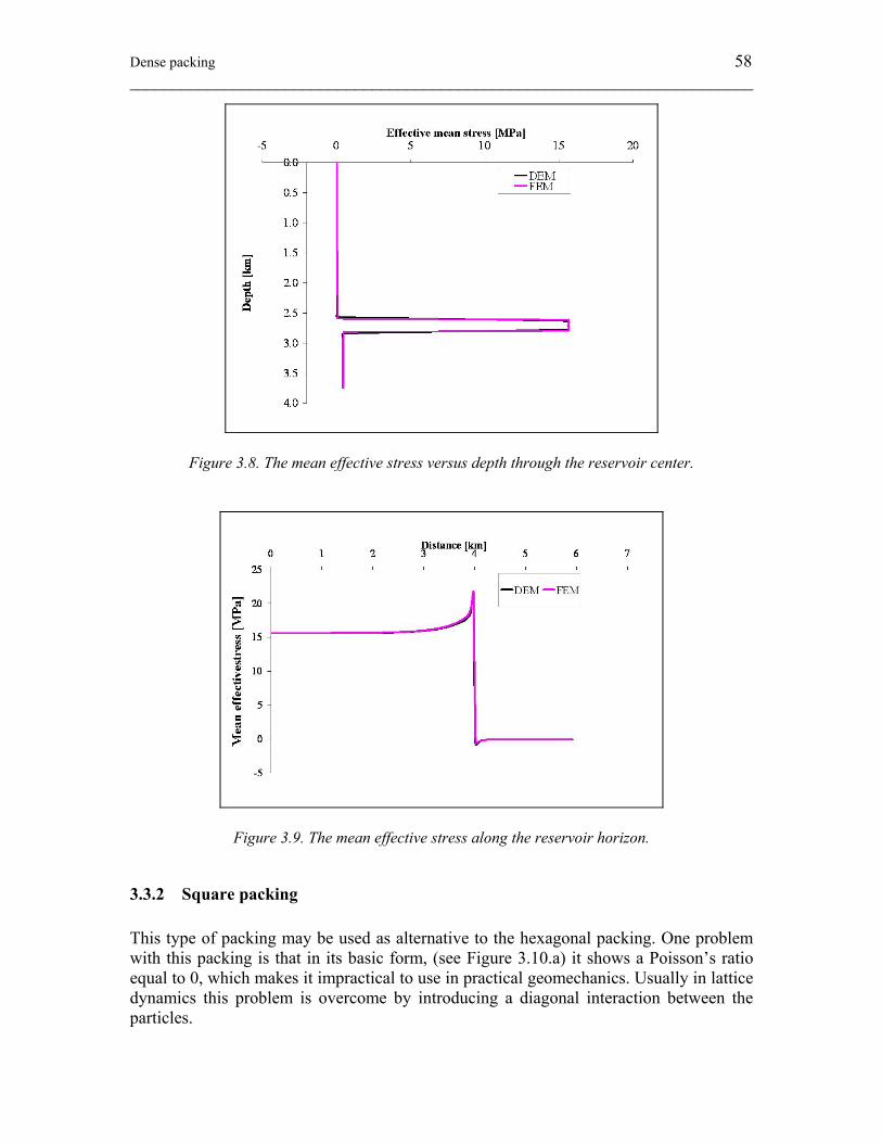
Dense packing 58 ________________________________________________________________________
Figure 3.8. The mean effective stress versus depth through the reservoir center.
Figure 3.9. The mean effective stress along the reservoir horizon.
3.3.2 Square packing This type of packing may be used as alternative to the hexagonal packing. One problem with this packing is that in its basic form, (see Figure 3.10.a) it shows a Poisson’s ratio equal to 0, which makes it impractical to use in practical geomechanics. Usually in lattice dynamics this problem is overcome by introducing a diagonal interaction between the particles.
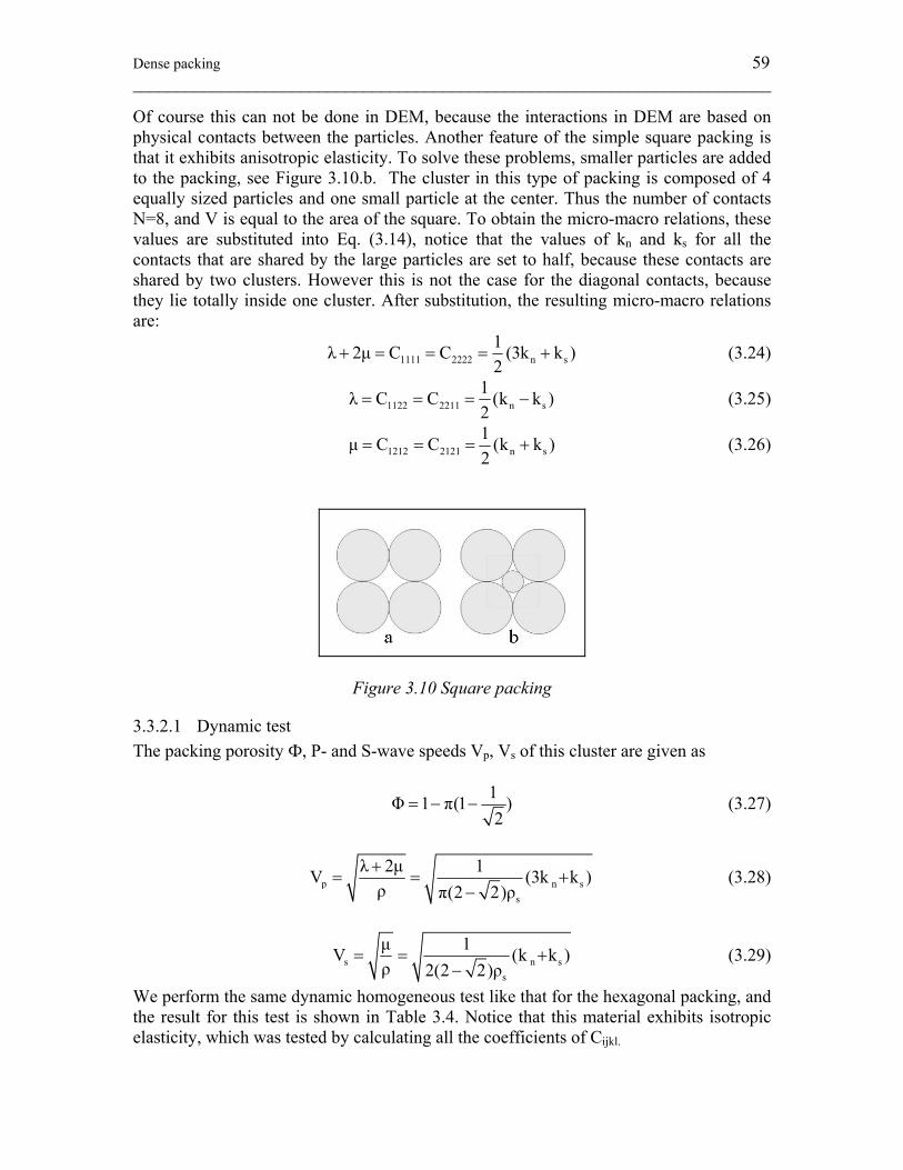
Dense packing 59 ________________________________________________________________________
Of course this can not be done in DEM, because the interactions in DEM are based on physical contacts between the particles. Another feature of the simple square packing is that it exhibits anisotropic elasticity. To solve these problems, smaller particles are added to the packing, see Figure 3.10.b. The cluster in this type of packing is composed of 4 equally sized particles and one small particle at the center. Thus the number of contacts N=8, and V is equal to the area of the square. To obtain the micro-macro relations, these values are substituted into Eq. (3.14), notice that the values of kn and ks for all the contacts that are shared by the large particles are set to half, because these contacts are shared by two clusters. However this is not the case for the diagonal contacts, because they lie totally inside one cluster. After substitution, the resulting micro-macro relations are:
1111 2222 n s1λ 2μ C C (3k k )2
+ = = = + (3.24)
1122 2211 n s1λ C C (k k )2
= = = − (3.25)
1212 2121 n s1μ C C (k k )2
= = = + (3.26)
Figure 3.10 Square packing
3.3.2.1 Dynamic test The packing porosity Ф, P- and S-wave speeds Vp, Vs of this cluster are given as
1Φ 1 π(1 )2
= − − (3.27)
p n ss
λ 2μ 1V (3k k )ρ π(2 2)ρ
+= = +
− (3.28)
s n ss
μ 1V (k k )ρ 2(2 2)ρ
= = +−
(3.29)
We perform the same dynamic homogeneous test like that for the hexagonal packing, and the result for this test is shown in Table 3.4. Notice that this material exhibits isotropic elasticity, which was tested by calculating all the coefficients of Cijkl.
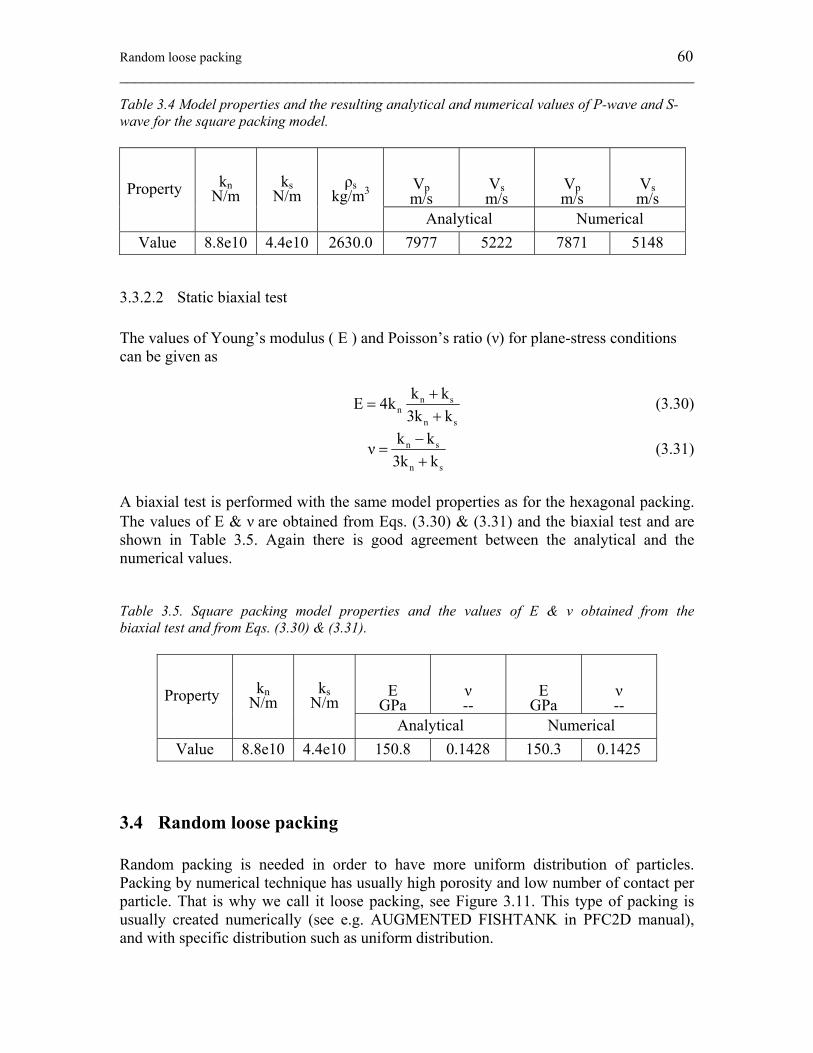
Random loose packing 60 ________________________________________________________________________
Table 3.4 Model properties and the resulting analytical and numerical values of P-wave and S-wave for the square packing model.
Vp m/s
Vs m/s
Vp m/s
Vs m/s Property kn
N/m ks
N/m ρs
kg/m3 Analytical Numerical
Value 8.8e10 4.4e10 2630.0 7977 5222 7871 5148
3.3.2.2 Static biaxial test The values of Young’s modulus ( E ) and Poisson’s ratio (ν) for plane-stress conditions can be given as
n sn
n s
k kE 4k3k k
+=
+ (3.30)
n s
n s
k kν3k k
−=
+ (3.31)
A biaxial test is performed with the same model properties as for the hexagonal packing. The values of E & ν are obtained from Eqs. (3.30) & (3.31) and the biaxial test and are shown in Table 3.5. Again there is good agreement between the analytical and the numerical values. Table 3.5. Square packing model properties and the values of E & ν obtained from the biaxial test and from Eqs. (3.30) & (3.31).
E GPa
ν --
E GPa
ν -- Property kn
N/m ks
N/m Analytical Numerical
Value 8.8e10 4.4e10 150.8 0.1428 150.3 0.1425
3.4 Random loose packing Random packing is needed in order to have more uniform distribution of particles. Packing by numerical technique has usually high porosity and low number of contact per particle. That is why we call it loose packing, see Figure 3.11. This type of packing is usually created numerically (see e.g. AUGMENTED FISHTANK in PFC2D manual), and with specific distribution such as uniform distribution.
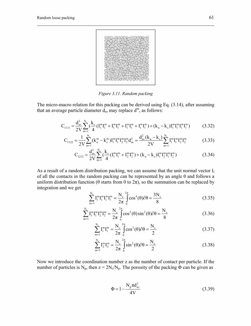
Random loose packing 61 ________________________________________________________________________
Figure 3.11. Random packing The micro-macro relation for this packing can be derived using Eq. (3.14), after assuming that an average particle diameter dav may replace dm, as follows:
cN2
m m m m m m m m m m m mav s1111 1 1 1 1 1 1 1 1 n s 1 1 1 1
m 1
d kC ( (I I I I I I I I ) (k k )I I I I )2V 4=
= + + + + −∑ (3.32)
c cN N2
m m m m m m 2 m m m mav n s1122 n s 1 1 2 2 m 1 1 2 2
m 1 m 1
d (k k )1C (k k )I I I I d I I I I2V 2V= =
−= − =∑ ∑ (3.33)
cN2
m m m m m m m mav s1212 1 1 2 2 n s 1 2 1 2
m 1
d kC ( (I I I I ) (k k )I I I I )2V 4=
= + + −∑ (3.34)
As a result of a random distribution packing, we can assume that the unit normal vector Ii of all the contacts in the random packing can be represented by an angle θ and follows a uniform distribution function (θ starts from 0 to 2π), so the summation can be replaced by integration and we get
c 2πN
m m m m 4c c1 1 1 1
m 1 0
N 3NI I I I cos (θ) θ2π 8=
= ∂ =∑ ∫ (3.35)
c 2πN
m m m m 2 2c c1 1 2 2
m 1 0
N NI I I I cos (θ)sin (θ) θ2π 8=
= ∂ =∑ ∫ (3.36)
c 2πN
m m 2c c1 1
m 1 0
N NI I cos (θ) θ2π 2=
= ∂ =∑ ∫ (3.37)
c 2πN
m m 2c c2 2
m 1 0
N NI I sin (θ) θ2π 2=
= ∂ =∑ ∫ (3.38)
Now we introduce the coordination number z as the number of contact per particle. If the number of particles is Np, then z = 2Nc/Np. The porosity of the packing Φ can be given as
2
p avN πdΦ 1
4V= − (3.39)
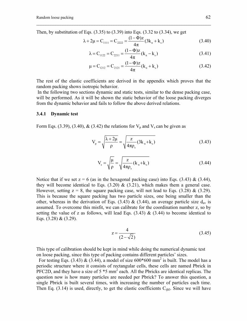
Random loose packing 62 ________________________________________________________________________
Then, by substitution of Eqs. (3.35) to (3.39) into Eqs. (3.32 to (3.34), we get
1111 2222 n s(1 Φ)zλ 2μ C C (3k k )
4π−
+ = = = + (3.40)
1122 2211 n s(1 Φ)zλ C C (k k )
4π−
= = = − (3.41)
1212 2121 n s(1 Φ)zμ C C (k k )
4π−
= = = + (3.42)
The rest of the elastic coefficients are derived in the appendix which proves that the random packing shows isotropic behavior. In the following two sections dynamic and static tests, similar to the dense packing case, will be performed. As it will be shown the static behavior of the loose packing diverges from the dynamic behavior and fails to follow the above derived relations.
3.4.1 Dynamic test Form Eqs. (3.39), (3.40), & (3.42) the relations for Vp and Vs can be given as
p n ss
λ 2μ zV (3k k )ρ 4πρ
+= = + (3.43)
s n ss
μ zV (k k )ρ 4πρ
= = + (3.44)
Notice that if we set z = 6 (as in the hexagonal packing case) into Eqs. (3.43) & (3.44), they will become identical to Eqs. (3.20) & (3.21), which makes them a general case. However, setting z = 8, the square packing case, will not lead to Eqs. (3.28) & (3.29). This is because the square packing has two particle sizes, one being smaller than the other, whereas in the derivation of Eqs. (3.43) & (3.44), an average particle size dav is assumed. To overcome this misfit, we can calibrate for the coordination number z, so by setting the value of z as follows, will lead Eqs. (3.43) & (3.44) to become identical to Eqs. (3.28) & (3.29).
4z(2 2)
=−
(3.45)
This type of calibration should be kept in mind while doing the numerical dynamic test on loose packing, since this type of packing contains different particles’ sizes. For testing Eqs. (3.43) & (3.44), a model of size 600*600 mm2 is built. The model has a periodic structure where it consists of rectangular cells, these cells are named Pbrick in PFC2D, and they have a size of 5 *5 mm2 each. All the Pbricks are identical replicas. The question now is how many particles are needed per Pbrick? To answer this question, a single Pbrick is built several times, with increasing the number of particles each time. Then Eq. (3.14) is used, directly, to get the elastic coefficients Cijkl. Since we will have
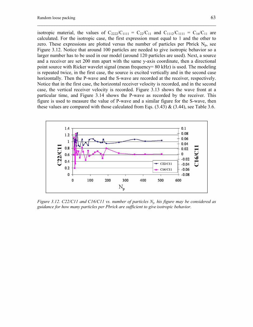
Random loose packing 63 ________________________________________________________________________
isotropic material, the values of C2222/C1111 = C22/C11 and C1112/C1111 = C16/C11 are calculated. For the isotropic case, the first expression must equal to 1 and the other to zero. These expressions are plotted versus the number of particles per Pbrick Np, see Figure 3.12. Notice that around 100 particles are needed to give isotropic behavior so a larger number has to be used in our model (around 120 particles are used). Next, a source and a receiver are set 200 mm apart with the same y-axis coordinate, then a directional point source with Ricker wavelet signal (mean frequency= 80 kHz) is used. The modeling is repeated twice, in the first case, the source is excited vertically and in the second case horizontally. Then the P-wave and the S-wave are recorded at the receiver, respectively. Notice that in the first case, the horizontal receiver velocity is recorded, and in the second case, the vertical receiver velocity is recorded. Figure 3.13 shows the wave front at a particular time, and Figure 3.14 shows the P-wave as recorded by the receiver. This figure is used to measure the value of P-wave and a similar figure for the S-wave, then these values are compared with those calculated from Eqs. (3.43) & (3.44), see Table 3.6.
Figure 3.12. C22/C11 and C16/C11 vs. number of particles Np. his figure may be considered as guidance for how many particles per Pbrick are sufficient to give isotropic behavior.
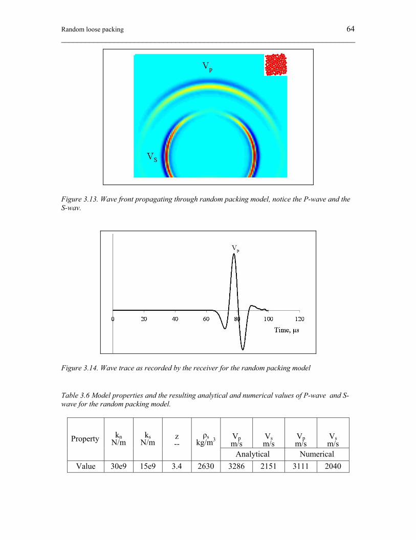
Random loose packing 64 ________________________________________________________________________
Figure 3.13. Wave front propagating through random packing model, notice the P-wave and the S-wav.
Figure 3.14. Wave trace as recorded by the receiver for the random packing model Table 3.6 Model properties and the resulting analytical and numerical values of P-wave and S-wave for the random packing model.
Vp m/s
Vs m/s
Vp m/s
Vs m/s Property kn
N/m ks
N/m
z --
ρs kg/m3
Analytical Numerical Value 30e9 15e9 3.4 2630 3286 2151 3111 2040
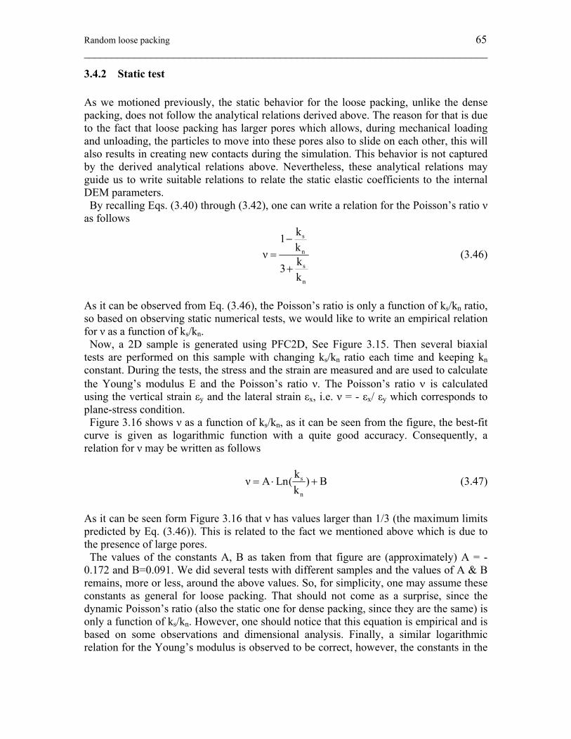
Random loose packing 65 ________________________________________________________________________
3.4.2 Static test As we motioned previously, the static behavior for the loose packing, unlike the dense packing, does not follow the analytical relations derived above. The reason for that is due to the fact that loose packing has larger pores which allows, during mechanical loading and unloading, the particles to move into these pores also to slide on each other, this will also results in creating new contacts during the simulation. This behavior is not captured by the derived analytical relations above. Nevertheless, these analytical relations may guide us to write suitable relations to relate the static elastic coefficients to the internal DEM parameters. By recalling Eqs. (3.40) through (3.42), one can write a relation for the Poisson’s ratio ν as follows
s
n
s
n
k1kν k3k
−=
+ (3.46)
As it can be observed from Eq. (3.46), the Poisson’s ratio is only a function of ks/kn ratio, so based on observing static numerical tests, we would like to write an empirical relation for ν as a function of ks/kn. Now, a 2D sample is generated using PFC2D, See Figure 3.15. Then several biaxial tests are performed on this sample with changing ks/kn ratio each time and keeping kn constant. During the tests, the stress and the strain are measured and are used to calculate the Young’s modulus E and the Poisson’s ratio ν. The Poisson’s ratio ν is calculated using the vertical strain εy and the lateral strain εx, i.e. ν = - εx/ εy which corresponds to plane-stress condition. Figure 3.16 shows ν as a function of ks/kn, as it can be seen from the figure, the best-fit curve is given as logarithmic function with a quite good accuracy. Consequently, a relation for ν may be written as follows
s
n
kν A Ln( ) Bk
= ⋅ + (3.47)
As it can be seen form Figure 3.16 that ν has values larger than 1/3 (the maximum limits predicted by Eq. (3.46)). This is related to the fact we mentioned above which is due to the presence of large pores. The values of the constants A, B as taken from that figure are (approximately) A = -0.172 and B=0.091. We did several tests with different samples and the values of A & B remains, more or less, around the above values. So, for simplicity, one may assume these constants as general for loose packing. That should not come as a surprise, since the dynamic Poisson’s ratio (also the static one for dense packing, since they are the same) is only a function of ks/kn. However, one should notice that this equation is empirical and is based on some observations and dimensional analysis. Finally, a similar logarithmic relation for the Young’s modulus is observed to be correct, however, the constants in the
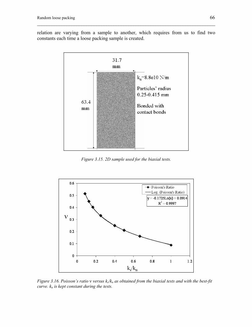
Random loose packing 66 ________________________________________________________________________
relation are varying from a sample to another, which requires from us to find two constants each time a loose packing sample is created.
Figure 3.15. 2D sample used for the biaxial tests.
Figure 3.16. Poisson’s ratio ν versus ks/kn as obtained from the biaxial tests and with the best-fit curve. kn is kept constant during the tests.
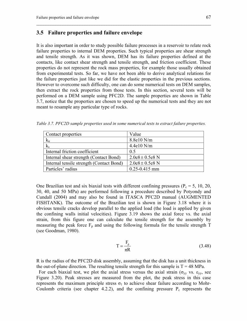
Failure properties and failure envelope 67 ________________________________________________________________________
3.5 Failure properties and failure envelope It is also important in order to study possible failure processes in a reservoir to relate rock failure properties to internal DEM properties. Such typical properties are shear strength and tensile strength. As it was shown, DEM has its failure properties defined at the contacts, like contact shear strength and tensile strength, and friction coefficient. These properties do not represent the rock mass properties, for example those usually obtained from experimental tests. So far, we have not been able to derive analytical relations for the failure properties just like we did for the elastic properties in the previous sections. However to overcome such difficulty, one can do some numerical tests on DEM samples, then extract the rock properties from those tests. In this section, several tests will be performed on a DEM sample using PFC2D. The sample properties are shown in Table 3.7, notice that the properties are chosen to speed up the numerical tests and they are not meant to resample any particular type of rocks. Table 3.7. PFC2D sample properties used in some numerical tests to extract failure properties.
Contact properties Value kn 8.8e10 N/m ks 4.4e10 N/m Internal friction coefficient 0.5 Internal shear strength (Contact Bond) 2.0e8 ± 0.5e8 N Internal tensile strength (Contact Bond) 2.0e8 ± 0.5e8 N Particles’ radius 0.25-0.415 mm
One Brazilian test and six biaxial tests with different confining pressures (Pc = 5, 10, 20, 30, 40, and 50 MPa) are performed following a procedure described by Potyondy and Cundall (2004) and may also be found in ITASCA PFC2D manual (AUGMENTED FISHTANK). The outcome of the Brazilian test is shown in Figure 3.18 where it is obvious tensile cracks develop parallel to the applied load (the load is applied by given the confining walls initial velocities). Figure 3.19 shows the axial force vs. the axial strain, from this figure one can calculate the tensile strength for the assembly by measuring the peak force Fp and using the following formula for the tensile strength T (see Goodman, 1980).
pFT
πR= (3.48)
R is the radius of the PFC2D disk assembly, assuming that the disk has a unit thickness in the out-of-plane direction. The resulting tensile strength for this sample is T = 48 MPa. For each biaxial test, we plot the axial stress versus the axial strain (σyy vs. εyy, see Figure 3.20). Peak stresses are measured from the plot, the peak stress in this case represents the maximum principle stress σ1 to achieve shear failure according to Mohr-Coulomb criteria (see chapter 4.2.2), and the confining pressure Pc represents the
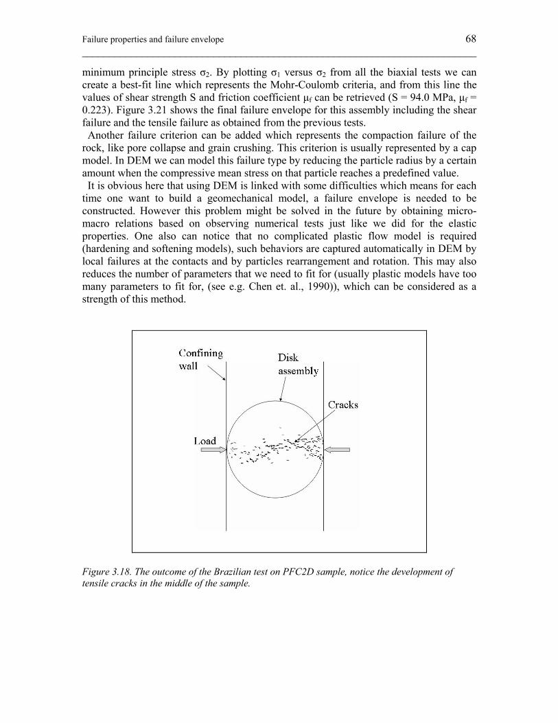
Failure properties and failure envelope 68 ________________________________________________________________________
minimum principle stress σ2. By plotting σ1 versus σ2 from all the biaxial tests we can create a best-fit line which represents the Mohr-Coulomb criteria, and from this line the values of shear strength S and friction coefficient μf can be retrieved (S = 94.0 MPa, μf = 0.223). Figure 3.21 shows the final failure envelope for this assembly including the shear failure and the tensile failure as obtained from the previous tests. Another failure criterion can be added which represents the compaction failure of the rock, like pore collapse and grain crushing. This criterion is usually represented by a cap model. In DEM we can model this failure type by reducing the particle radius by a certain amount when the compressive mean stress on that particle reaches a predefined value. It is obvious here that using DEM is linked with some difficulties which means for each time one want to build a geomechanical model, a failure envelope is needed to be constructed. However this problem might be solved in the future by obtaining micro-macro relations based on observing numerical tests just like we did for the elastic properties. One also can notice that no complicated plastic flow model is required (hardening and softening models), such behaviors are captured automatically in DEM by local failures at the contacts and by particles rearrangement and rotation. This may also reduces the number of parameters that we need to fit for (usually plastic models have too many parameters to fit for, (see e.g. Chen et. al., 1990)), which can be considered as a strength of this method.
Figure 3.18. The outcome of the Brazilian test on PFC2D sample, notice the development of tensile cracks in the middle of the sample.
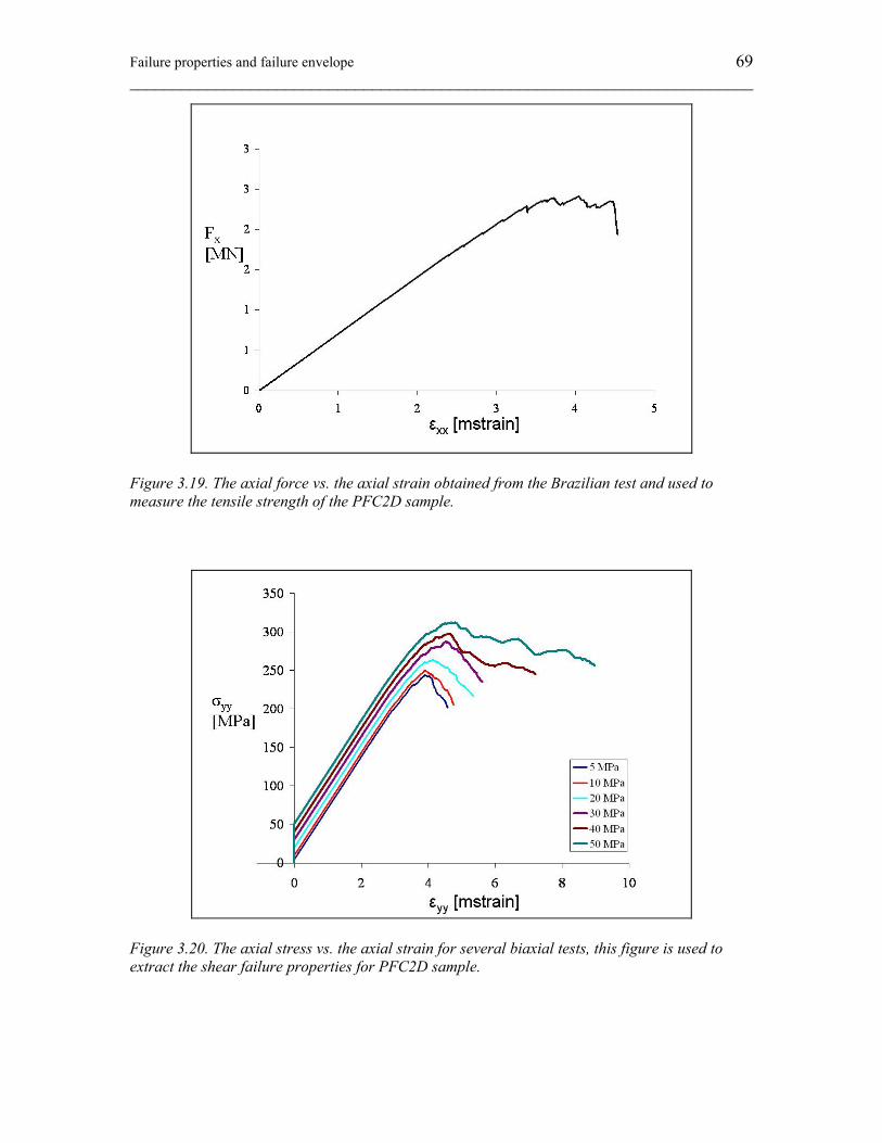
Failure properties and failure envelope 69 ________________________________________________________________________
Figure 3.19. The axial force vs. the axial strain obtained from the Brazilian test and used to measure the tensile strength of the PFC2D sample.
Figure 3.20. The axial stress vs. the axial strain for several biaxial tests, this figure is used to extract the shear failure properties for PFC2D sample.
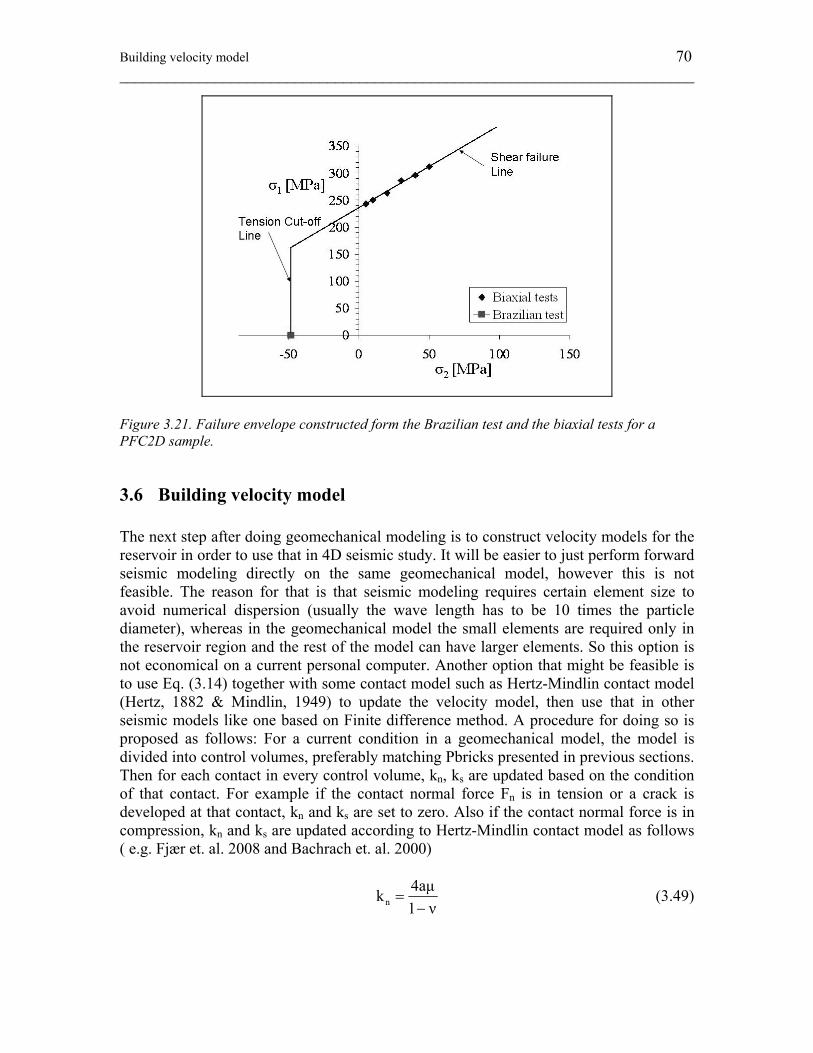
Building velocity model 70 ________________________________________________________________________
Figure 3.21. Failure envelope constructed form the Brazilian test and the biaxial tests for a PFC2D sample.
3.6 Building velocity model The next step after doing geomechanical modeling is to construct velocity models for the reservoir in order to use that in 4D seismic study. It will be easier to just perform forward seismic modeling directly on the same geomechanical model, however this is not feasible. The reason for that is that seismic modeling requires certain element size to avoid numerical dispersion (usually the wave length has to be 10 times the particle diameter), whereas in the geomechanical model the small elements are required only in the reservoir region and the rest of the model can have larger elements. So this option is not economical on a current personal computer. Another option that might be feasible is to use Eq. (3.14) together with some contact model such as Hertz-Mindlin contact model (Hertz, 1882 & Mindlin, 1949) to update the velocity model, then use that in other seismic models like one based on Finite difference method. A procedure for doing so is proposed as follows: For a current condition in a geomechanical model, the model is divided into control volumes, preferably matching Pbricks presented in previous sections. Then for each contact in every control volume, kn, ks are updated based on the condition of that contact. For example if the contact normal force Fn is in tension or a crack is developed at that contact, kn and ks are set to zero. Also if the contact normal force is in compression, kn and ks are updated according to Hertz-Mindlin contact model as follows ( e.g. Fjær et. al. 2008 and Bachrach et. al. 2000)
n4aμk1 ν
=−
(3.49)
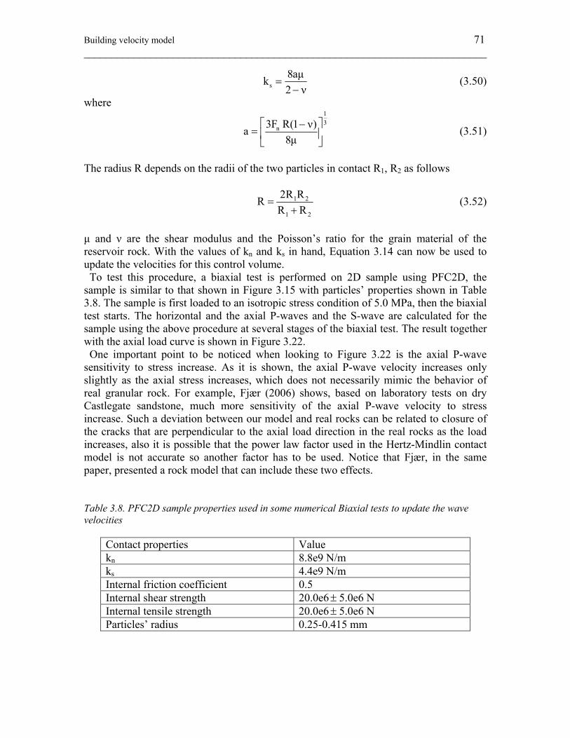
Building velocity model 71 ________________________________________________________________________
s8aμk2 ν
=−
(3.50)
where
13
n3F R(1 ν)a8μ
⎡ ⎤−= ⎢ ⎥
⎣ ⎦ (3.51)
The radius R depends on the radii of the two particles in contact R1, R2 as follows
1 2
1 2
2R RRR R
=+
(3.52)
μ and ν are the shear modulus and the Poisson’s ratio for the grain material of the reservoir rock. With the values of kn and ks in hand, Equation 3.14 can now be used to update the velocities for this control volume. To test this procedure, a biaxial test is performed on 2D sample using PFC2D, the sample is similar to that shown in Figure 3.15 with particles’ properties shown in Table 3.8. The sample is first loaded to an isotropic stress condition of 5.0 MPa, then the biaxial test starts. The horizontal and the axial P-waves and the S-wave are calculated for the sample using the above procedure at several stages of the biaxial test. The result together with the axial load curve is shown in Figure 3.22. One important point to be noticed when looking to Figure 3.22 is the axial P-wave sensitivity to stress increase. As it is shown, the axial P-wave velocity increases only slightly as the axial stress increases, which does not necessarily mimic the behavior of real granular rock. For example, Fjær (2006) shows, based on laboratory tests on dry Castlegate sandstone, much more sensitivity of the axial P-wave velocity to stress increase. Such a deviation between our model and real rocks can be related to closure of the cracks that are perpendicular to the axial load direction in the real rocks as the load increases, also it is possible that the power law factor used in the Hertz-Mindlin contact model is not accurate so another factor has to be used. Notice that Fjær, in the same paper, presented a rock model that can include these two effects. Table 3.8. PFC2D sample properties used in some numerical Biaxial tests to update the wave velocities
Contact properties Value kn 8.8e9 N/m ks 4.4e9 N/m Internal friction coefficient 0.5 Internal shear strength 20.0e6 ± 5.0e6 N Internal tensile strength 20.0e6 ± 5.0e6 N Particles’ radius 0.25-0.415 mm
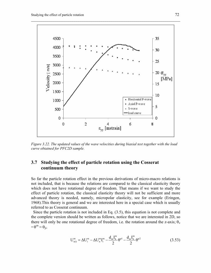
Studying the effect of particle rotation 72 ________________________________________________________________________
Figure 3.22. The updated values of the wave velocities during biaxial test together with the load curve obtained for PFC2D sample.
3.7 Studying the effect of particle rotation using the Cosserat continuum theory
So far the particle rotation effect in the previous derivations of micro-macro relations is not included, that is because the relations are compared to the classical elasticity theory which does not have rotational degree of freedom. That means if we want to study the effect of particle rotation, the classical elasticity theory will not be sufficient and more advanced theory is needed, namely, micropolar elasticity, see for example (Eringen, 1968).This theory is general and we are interested here in a special case which is usually referred to as Cosserat continuum. Since the particle rotation is not included in Eq. (3.5), this equation is not complete and the complete version should be written as follows, notice that we are interested in 2D, so there will only be one rotational degree of freedom, i.e. the rotation around the z-axis; θz
= θm ≈ θji.
m m
m m m m p1 p2m k m ks(i) i n i
d I d IU ΔU ΔU I θ θ2 2
= − − − (3.53)
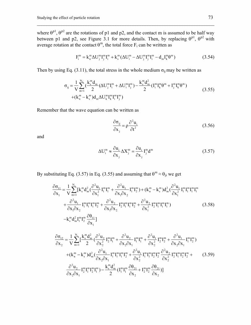
Studying the effect of particle rotation 73 ________________________________________________________________________
where θp1, θp2 are the rotations of p1 and p2, and the contact m is assumed to be half way between p1 and p2, see Figure 3.1 for more details. Then, by replacing θp1, θp2 with average rotation at the contact θm, the total force Fi can be written as m m m m m m m m m m m m
i n j j i s i j j i m kF k ΔU I I k (ΔU ΔU I I d I θ )= + − − (3.54) Then by using Eq. (3.11), the total stress in the whole medium σij may be written as
CN m m 2m m m m m m m m m ms m s m
ij j i i j i k j km 1m m m m m mn s m k k i j
k d k d1σ ( (ΔU I ΔU I ) (I I θ I I θ )V 2 2(k k )d ΔU I I I )
=
= + − +
+ −
∑ (3.55)
Remember that the wave equation can be written as
2
ij i2
j
σ uρx t
∂ ∂=
∂ ∂ (3.56)
and
m m m mi ii j j
j j
u uΔU ΔX I dx x
∂ ∂≈ =
∂ ∂ (3.57)
By substituting Eq. (3.57) in Eq. (3.55) and assuming that θm ≈ θji we get
cN 2 2 2m 2 m m m m m m 2 m m m m11 1 1 1s m 1 1 1 2 n s m 1 1 1 12 2
m 11 1 1 2 12 2 2
m m m m m m m m m m m m1 2 21 1 1 2 2 1 1 2 2 1 1 12
1 2 1 2 1
m 2 m m 11s m 1 2
1
σ u u u1 [k d ( I I I I ) (k k )d ( I I I Ix V x x x x
u u uI I I I I I I I I I I I )x x x x x
θk d I I ]x
=
∂ ∂ ∂ ∂= + + −
∂ ∂ ∂ ∂ ∂
∂ ∂ ∂+ + +
∂ ∂ ∂ ∂ ∂∂
−∂
∑
(3.58)
cN m 2 2 2 2 2m m m m m m m ms m12 2 2 1 12 1 1 1 2 2 1 22 2
m 12 2 2 1 2 2 12 2 2
m m 2 m m m m m m m m m m m m1 1 2n s m 1 1 1 2 1 1 2 2 2 1 2 22 2
2 1 2 2m 22
m m m m s m22 1 2 1
2 1
k dσ u u u u1 [ ( I I I I I I I I )x V 2 x x x x x x
u u u(k k )d ( I I I I I I I I I I I Ix x x x
k du I I I I ) (Ix x 2
=
∂ ∂ ∂ ∂ ∂= + + +
∂ ∂ ∂ ∂ ∂ ∂ ∂
∂ ∂ ∂+ − + +
∂ ∂ ∂ ∂
∂−
∂ ∂
∑
m m m m21 211 1 2 2
2 2
θ θI I I )]x x
∂ ∂+
∂ ∂
(3.59)
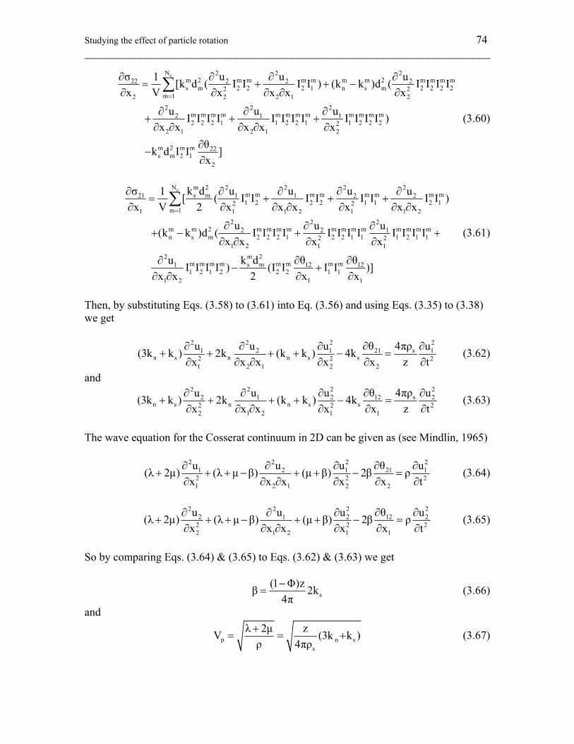
Studying the effect of particle rotation 74 ________________________________________________________________________
cN 2 2 2m 2 m m m m m m 2 m m m m22 2 2 2s m 2 2 2 1 n s m 2 2 2 22 2
m 12 2 2 1 22 2 2
m m m m m m m m m m m m2 1 12 2 2 1 1 2 2 1 1 2 2 22
2 1 2 1 2
m 2 m m 22s m 2 1
2
σ u u u1 [k d ( I I I I ) (k k )d ( I I I Ix V x x x x
u u uI I I I I I I I I I I I )x x x x x
θk d I I ]x
=
∂ ∂ ∂ ∂= + + −
∂ ∂ ∂ ∂ ∂
∂ ∂ ∂+ + +
∂ ∂ ∂ ∂ ∂∂
−∂
∑
(3.60)
cN m 2 2 2 2 2m m m m m m m ms m21 1 1 2 21 2 2 2 1 1 2 12 2
m 11 1 1 2 1 1 22 2 2
m m 2 m m m m m m m m m m m m2 2 1n s m 2 2 2 1 2 2 1 1 1 2 1 12 2
1 2 1 1m 22
m m m m s m11 2 1 2
1 2
k dσ u u u u1 [ ( I I I I I I I I )x V 2 x x x x x x
u u u(k k )d ( I I I I I I I I I I I Ix x x x
k du I I I I ) (Ix x 2
=
∂ ∂ ∂ ∂ ∂= + + +
∂ ∂ ∂ ∂ ∂ ∂ ∂
∂ ∂ ∂+ − + +
∂ ∂ ∂ ∂
∂−
∂ ∂
∑
m m m m12 122 2 1 1
1 1
θ θI I I )]x x
∂ ∂+
∂ ∂
(3.61)
Then, by substituting Eqs. (3.58) to (3.61) into Eq. (3.56) and using Eqs. (3.35) to (3.38) we get
2 2 2 2
s1 2 1 21 1n s n n s s2 2 2
1 2 1 2 2
4πρu u u θ u(3k k ) 2k (k k ) 4kx x x x x z t
∂ ∂ ∂ ∂ ∂+ + + + − =
∂ ∂ ∂ ∂ ∂ ∂ (3.62)
and
2 2 2 2
s2 1 2 12 2n s n n s s2 2 2
2 1 2 1 1
4πρu u u θ u(3k k ) 2k (k k ) 4kx x x x x z t
∂ ∂ ∂ ∂ ∂+ + + + − =
∂ ∂ ∂ ∂ ∂ ∂ (3.63)
The wave equation for the Cosserat continuum in 2D can be given as (see Mindlin, 1965)
2 2 2 2
1 2 1 21 12 2 21 2 1 2 2
u u u θ u(λ 2μ) (λ μ β) (μ β) 2β ρx x x x x t
∂ ∂ ∂ ∂ ∂+ + + − + + − =
∂ ∂ ∂ ∂ ∂ ∂ (3.64)
2 2 2 2
2 1 2 12 22 2 22 1 2 1 1
u u u θ u(λ 2μ) (λ μ β) (μ β) 2β ρx x x x x t
∂ ∂ ∂ ∂ ∂+ + + − + + − =
∂ ∂ ∂ ∂ ∂ ∂ (3.65)
So by comparing Eqs. (3.64) & (3.65) to Eqs. (3.62) & (3.63) we get
s(1 Φ)zβ 2k
4π−
= (3.66)
and
p n ss
λ 2μ zV (3k k )ρ 4πρ
+= = + (3.67)

Studying the effect of particle rotation 75 ________________________________________________________________________
s n ss
μ β zV (k k )ρ 4πρ+
= = + (3.68)
Notice that this result is the same like that derived previously. Now, if the particles are not allowed to rotate (i.e. constrain the particles rotation θ = 0), Eqs. (3.62) & (3.63) will
become equivalent to those of classical continuum which means cn s
(1 Φ)zμ (k k )4π−
= + ,
and cn s
(1 Φ)zλ (k k )4π−
= − , where “c” stands for “constrained”. However β is not zero and
still given by Eq. (3.66), that means the shear wave is given as
c
s n ss
μ β zV (k 3k )ρ 4πρ+
= = + (3.69)
and
c c
p n ss
λ 2μ zV (3k k )ρ 4πρ
+= = + (3.70)
If one compares Eq. (3.69) to Eq. (3.70) (or Eq. (3.67)), it can be seen that when ks > kn, Vs will be larger than Vp, which is unrealistic to isotropic elastic solid. However this behavior is a consequence of imposing a constrain on the particle rotation in the numerical model, which is considered unrealistic condition in real rocks (e.g. sandstone), because grains in these rocks do rotate. Finally, to test Eq. (3.69), a DEM model using PFC2D is built where ks is set three times the value of kn, then waves are allowed to propagate inside the model by applying directional force source. Figure 3.23 shows the wave front; notice how Vs propagates faster than Vp as predicted by Eq. (3.69).
Figure 3.23. Wave front propagating inside DEM 2D Model where the particles are not allowed to rotate and ks = 3kn, notice how the S-wave propagates faster than the P-wave.

76 ________________________________________________________________________
Chapter 4: A modified discrete element approach 77 ________________________________________________________________________
4 A modified discrete element approach
4.1 Introduction In the previous chapters (2 & 3) we show the potential of using DEM in both geomechanical modeling and seismic forward modeling, also a general technique to relate its internal constitutive parameters such as kn, ks to the conventional constitutive parameters such Young’s Modulus, Poisson’s Ratio, and the wave velocities Vp, and Vs is presented. The approach still has, first, a problem when it comes to feed the model with strength properties which are stress-based in the real life and are contact force-based in DEM. As it was shown, some numerical tests are needed to construct the failure envelope. Second, it is more difficult to construct a model and install initial conditions, like stress, using DEM than in the other well-established methods such as Finite Element (FEM) or Finite Difference Methods (FDM). Third, as it was shown in Chapter 3, DEM has a limitation on the maximum Vp/Vs ratio (limited by 3 ). Because of these hindrances, we decided to make some modifications on the original DEM. The modified approach works with clusters, where each cluster is made of three elements, unlike the original DEM which works with single element. At this stage the shear stiffness ks is neglected. Next the solution scheme for this approach is presented. Also a relation between the stress and the internal forces is obtained which enable us to define the failure properties just like in other continuum methods such as FEM, and FDM, and install the initial condition easily. Each cluster can have one of three states, intact cluster which behaves similar to FEM or DEM, failing cluster which behaves exactly like DEM, and interface cluster which is used to model faults and predefined fractures. The approach may be considered similar to other methods that work with fracturing like Numerical Manifold Method (Shi, 1991), The Combined Finite-Discrete element method (Munjiza, 2004), AC/DC in PFC2D v4.0 (Itasca Consultant Group). It should be mentioned that the theory behind this approach is based on DEM as presented by Cundall (1979). After that, the elastic behavior of this approach is compared to FEM using a simple reservoir geomechanical example. Also some fracture propagation examples are shown, the first example shows how the fracture propagates from the tips of initial horizontal crack during tensile test, and the second shows how wing-fractures are developed at the tips of inclined crack during compressive test. The final example shows the developments of the shear bands during biaxial test. These tests are done for validation. Then, a general approach is presented where ks is included. By including ks, the approach becomes more close to the original DEM. Also, with ks being included, element rotation has to be included. This of course raises the demand of computer power, however element rotation can affect fracture propagation and sliding (Liebowitz, 1968 & Ehlers, 2003), which might be interesting to see. Finally, fluid coupled method is presented based on Finite different method where the spatial discretization is achieved by a network of pipes. The method allows flow through fractures as they are developed in the geomechanical model.
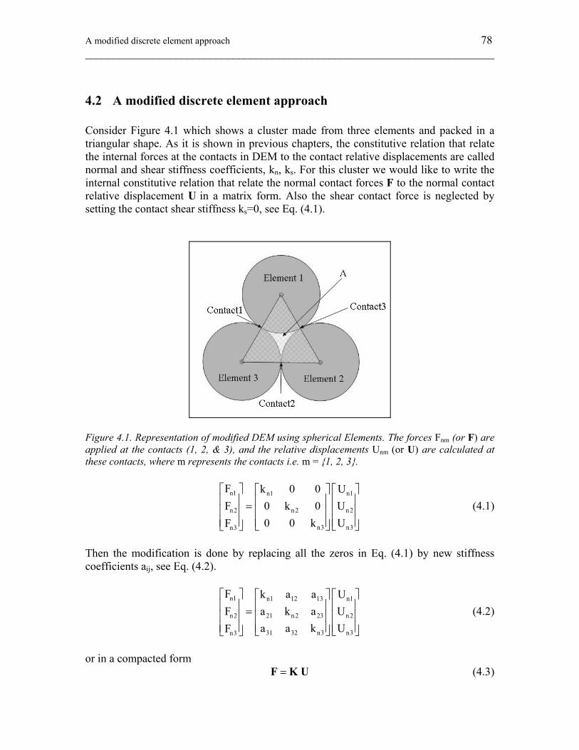
A modified discrete element approach 78 ________________________________________________________________________
4.2 A modified discrete element approach Consider Figure 4.1 which shows a cluster made from three elements and packed in a triangular shape. As it is shown in previous chapters, the constitutive relation that relate the internal forces at the contacts in DEM to the contact relative displacements are called normal and shear stiffness coefficients, kn, ks. For this cluster we would like to write the internal constitutive relation that relate the normal contact forces F to the normal contact relative displacement U in a matrix form. Also the shear contact force is neglected by setting the contact shear stiffness ks=0, see Eq. (4.1).
Figure 4.1. Representation of modified DEM using spherical Elements. The forces Fnm (or F) are applied at the contacts (1, 2, & 3), and the relative displacements Unm (or U) are calculated at these contacts, where m represents the contacts i.e. m = {1, 2, 3}.
n1 n1 n1
n2 n2 n2
n3 n3n3
F k 0 0 UF 0 k 0 U
0 0 k UF
⎡ ⎤ ⎡ ⎤ ⎡ ⎤⎢ ⎥ ⎢ ⎥ ⎢ ⎥=⎢ ⎥ ⎢ ⎥ ⎢ ⎥⎢ ⎥ ⎢ ⎥ ⎢ ⎥⎣ ⎦ ⎣ ⎦⎣ ⎦
(4.1)
Then the modification is done by replacing all the zeros in Eq. (4.1) by new stiffness coefficients aij, see Eq. (4.2).
n1 n1 12 13 n1
n2 21 n2 23 n2
31 32 n3 n3n3
F k a a UF a k a U
a a k UF
⎡ ⎤ ⎡ ⎤ ⎡ ⎤⎢ ⎥ ⎢ ⎥ ⎢ ⎥=⎢ ⎥ ⎢ ⎥ ⎢ ⎥⎢ ⎥ ⎢ ⎥ ⎢ ⎥⎣ ⎦ ⎣ ⎦⎣ ⎦
(4.2)
or in a compacted form F K U= (4.3)
A modified discrete element approach 79 ________________________________________________________________________
Remember that the stress σ = [σxx, σyy , σxy] may be written as a function of internal force as follows (recall Eq. (3.11))
2 2 2xx 11 1 21 2 31 3 n1
2 2 2yy 12 1 22 2 32 3 n2
xy 11 12 1 21 22 2 31 32 3 n3
I d I d I d F1 I d I d I d FA
I I d I I d I I d F
⎡ ⎤⎡ ⎤σ ⎡ ⎤⎢ ⎥⎢ ⎥ ⎢ ⎥σ = ⎢ ⎥⎢ ⎥ ⎢ ⎥⎢ ⎥⎢ ⎥ ⎢ ⎥σ ⎣ ⎦⎣ ⎦ ⎣ ⎦
(4.5)
or
1A
Tσ= M F (4.6)
A relation for the strain ε = [εxx, εyy, εxy] can be given by using Eqs. (3.4), (3.6), & (3.7) as
1 2 2xxn 11 1 12 1 11 12 1
2 2 2n 21 2 22 2 21 22 2 yy3 2 2 2n 31 3 32 3 31 32 3 xy
U I d I d I I dU I d I d I I dU I d I d I I d
⎡ ⎤⎡ ⎤ ⎡ ⎤ ε⎢ ⎥⎢ ⎥ ⎢ ⎥= ε⎢ ⎥⎢ ⎥ ⎢ ⎥⎢ ⎥⎢ ⎥ ⎢ ⎥ ε⎣ ⎦ ⎣ ⎦ ⎣ ⎦
(4.7)
or U= M ε (4.8) Remember also σ Cε= (4.9) So by using Eqs. (4.2), (4.5), (4.7), & (4.9), one may write (see also Ferrari et. al., 1997)
2 2 2 2 211 1 21 2 31 3 11 1 12 1 11 12 111 12 14 n1 12 132 2 2 2 2
21 22 24 12 1 22 2 32 3 21 n2 23 21 2 22 2 21 22 22 241 42 44 11 12 1 21 22 2 31 32 3 31 32 n3 31 3 32
I d I d I d I d I d I I dC C C k a a1C C C I d I d I d a k a I d I d I I dA
C C C I I d I I d I I d a a k I d I d
⎡ ⎤ ⎡ ⎤⎡ ⎤ ⎢ ⎥ ⎢ ⎥⎢ ⎥ ⎢ ⎥= ⎢ ⎥⎢ ⎥ ⎢ ⎥ ⎢ ⎥⎢ ⎥ ⎢ ⎥⎣ ⎦ ⎣ ⎦⎣ ⎦ 3 31 32 3I I d
⎡ ⎤⎢ ⎥⎢ ⎥⎢ ⎥⎢ ⎥⎣ ⎦
(4.10)
or in compacted form
T1C= M K MA
(4.11)
where K is the internal (cluster) constitutive relations (or micro-stiffness matrix), C is the material constitutive relations (or macro-stiffness matrix). A is the area of the cluster (or triangle), and the area is used instead of the volume, since we assume that each cluster has a unit thickness (in the out-of-plane direction), this will guarantee that the stress in Eq. (4.5) has the right unit. M is the unit normal vector matrix for the cluster, and Im1=cosθm, and Im2=sinθm, and the angle θm represents the normal vector orientation of the contact m inside the cluster. dm is the contact’s length (the distance between the two elements that are in contact).
A modified discrete element approach 80 ________________________________________________________________________
It is also possible to write Eqs. (4.10) & (4.11) in a different form as follows
1A
=C M'K (4.12)
where T
n1 12 13 21 n 2 23 31 32 n3[k a a a k a a a k ]=K is written in a vector
form instead, similarly [ ]T
11 12 14 21 22 24 41 42 44c c c c c c c c cC = . And M' is defined as
4 2 2 2 2 2 2 2 4 2 2 2 2 2 2 2 4 211 1 11 21 1 2 11 31 1 3 21 11 2 1 21 2 21 31 2 3 31 11 3 1 31 21 3 2 31 3
2 2 2 2 2 2 2 2 2 2 2 2 2 2 2 2 2 2 2 211 12 1 11 22 1 2 11 32 1 3 21 12 2 1 21 22 2 21 32 2 3 31 12 3 1 31 22 3 2 31 32 3
I d I I d d I I d d I I d d I d I I d d I I d d I I d d I d
I I d I I d d I I d d I I d d I I d I I d d I I d d I I d d I I d
=M'
2
3 2 2 2 2 3 2 2 2 2 3 211 12 1 11 21 22 1 2 11 31 32 1 3 21 11 12 2 1 21 22 2 21 31 32 2 3 31 11 12 3 1 31 21 22 3 2 31 32 32 212 11 12 21 1 2 12 31 1 3 22 11 2 1 22 21 2 22 31 2 3 32 11 3 1 32
2 2 2 2 2 2 2 2 2 2 2 2 2 21
I I d I I I d d I I I d d I I I d d I I d I I I d d I I I d d I I I d d I I d
I I I I d d I I d d I I d d I I d I I d d I I d d Id 221 3 2 32 31 3
2 2 2 2 2 2 2 2 4 212 12 22 1 2 12 32 1 3 22 12 2 1 22 2 2 22 32 2 3 32 12 3 1 32 22 3 2 32 3
2 2 2 2 3 2 212 11 1 12 2
2 2 2 2
4 2 2 2 2 2
1 22 1 2 12 31 32 1 3 22 11 12 2 1 22 21 2 22 31 3
2 2 41
3 22 2 3 32 11
I d d I I d
I I I d d I I d d I I d d I d d I I d d I I d d I I d d I d
I I d I I I d d I I I d d I I I d d I I d I I I d d I I
d
I 2 3 212 3 1 32 21 22 3 2 32 31 3
3 2 2 2 2 3 2 2 2 2 3 211 12 1 11 12 21 1 2 11 12 31 1 3 21 22 11 2 1 21 22 2 21 22 31 2 3 31 32 11 3 1 31 32 21 3 2 31 32 3
2 2 2 211 12 12 1 11 12 22 1 2 11 12 32 1 3 21 22 12 2 1
2
d d I I I d d I I d
I I d I I I d d I I I d d I I I d d I I d I I I d d I I I d d I I I d d I I d
I I I d I I I d d I I I d d I I I d d I2 2 2 2 2 2
1 11 12 21 22 11 12 31 32 21 22 11 12 21 22 31 32 31 32 11
2 2 2 2 2 3 221 22 22 2 21 22 32 2 3 31 32 12 3 1 31 32 22 3 2 31 32 3
2 2 211 12 1 2 1 3 2 1 21 22 2 2 3 3 112 31 32 3 2 321 2 12 32 3d I I I I I I I I
I I d I I I d d I I I d d I I I d d I I d
I I d d d d d d I I d d d d d d d I II I I I I I I I I I I I I I dI I
⎡⎢⎢⎢⎢⎢
⎣
⎤⎥⎥⎥⎥⎥
⎢ ⎥⎢ ⎥⎢ ⎥⎢ ⎥⎢ ⎥⎢ ⎥⎢ ⎥⎢ ⎥⎢ ⎥⎢ ⎥⎦
(4.13)
Notice that the elements are not necessary spherical, they can follow Voronoi’s shapes, which makes it easier to build more complicated models with the help of automatic mesh generation codes, see Figure 4.2. In the right side of this figure a cluster taken from the triangular mesh (or Voronoi’s diagram) is shown. The cluster has three edges (Eg1, Eg2, Eg3), this is true for any cluster made from such a triangular mesh and thus guarantees the applicability of above formulation. The figure also shows the unit normal vectors: I1i, I2i, and I3i used in the above formulation. Notice that columns (1, 5, & 9) in Eq. (4.13) can be obtained directly from Equation (3.14), whereas the rest are obtained as a result of introducing the new stiffness coefficients aij. In regular DEM these columns are set to zero. It is worth to mention that K in Eq. (4.11) is equivalent to element stiffness matrix Ke derived in Finite Element Method (FEM), where it is given as (see, for example, Kwon & Bang, 1997). e T AK B C B = where B is a shape function matrix. Notice our derivation is based 100 % on the Particle-Based Discrete Element Method as developed by Cundall, unlike the Finite Element Method where the derivation of the stiffness matrix is based on simplifying partial deferential equation using specific shape function. In fact, Hori et. al. (2005) derived a special shape function based on DEM and they showed that it is equal to linear shape function of triangular finite element, they called the method FEM-β. So in this case Ke ~ K, and B ~ M-1, where (-1) means the inverse. Later on, we will present a general modified DEM approach where ks will be included, in that case we may not expect that the resulted derivations will be equivalent to any FEM derivations.
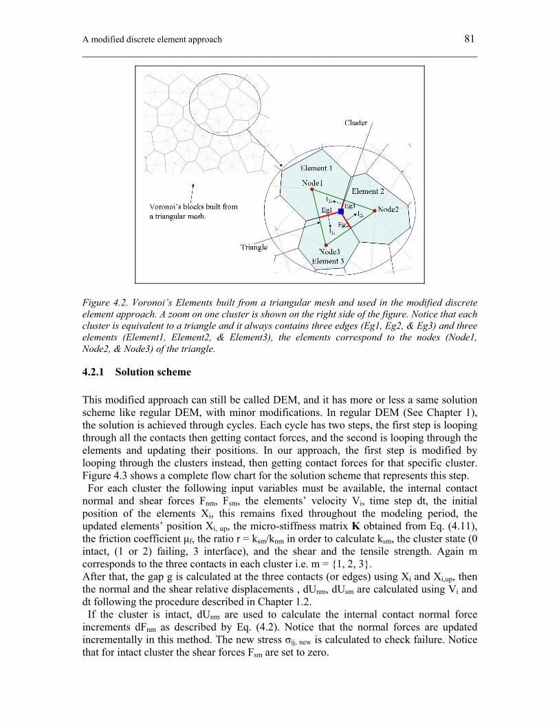
A modified discrete element approach 81 ________________________________________________________________________
Figure 4.2. Voronoi’s Elements built from a triangular mesh and used in the modified discrete element approach. A zoom on one cluster is shown on the right side of the figure. Notice that each cluster is equivalent to a triangle and it always contains three edges (Eg1, Eg2, & Eg3) and three elements (Element1, Element2, & Element3), the elements correspond to the nodes (Node1, Node2, & Node3) of the triangle.
4.2.1 Solution scheme This modified approach can still be called DEM, and it has more or less a same solution scheme like regular DEM, with minor modifications. In regular DEM (See Chapter 1), the solution is achieved through cycles. Each cycle has two steps, the first step is looping through all the contacts then getting contact forces, and the second is looping through the elements and updating their positions. In our approach, the first step is modified by looping through the clusters instead, then getting contact forces for that specific cluster. Figure 4.3 shows a complete flow chart for the solution scheme that represents this step. For each cluster the following input variables must be available, the internal contact normal and shear forces Fnm, Fsm, the elements’ velocity Vi, time step dt, the initial position of the elements Xi, this remains fixed throughout the modeling period, the updated elements’ position Xi, up, the micro-stiffness matrix K obtained from Eq. (4.11), the friction coefficient μf, the ratio r = ksm/knm in order to calculate ksm, the cluster state (0 intact, (1 or 2) failing, 3 interface), and the shear and the tensile strength. Again m corresponds to the three contacts in each cluster i.e. m = {1, 2, 3}. After that, the gap g is calculated at the three contacts (or edges) using Xi and Xi,up, then the normal and the shear relative displacements , dUnm, dUsm are calculated using Vi and dt following the procedure described in Chapter 1.2. If the cluster is intact, dUnm are used to calculate the internal contact normal force increments dFnm as described by Eq. (4.2). Notice that the normal forces are updated incrementally in this method. The new stress σij, new is calculated to check failure. Notice that for intact cluster the shear forces Fsm are set to zero.
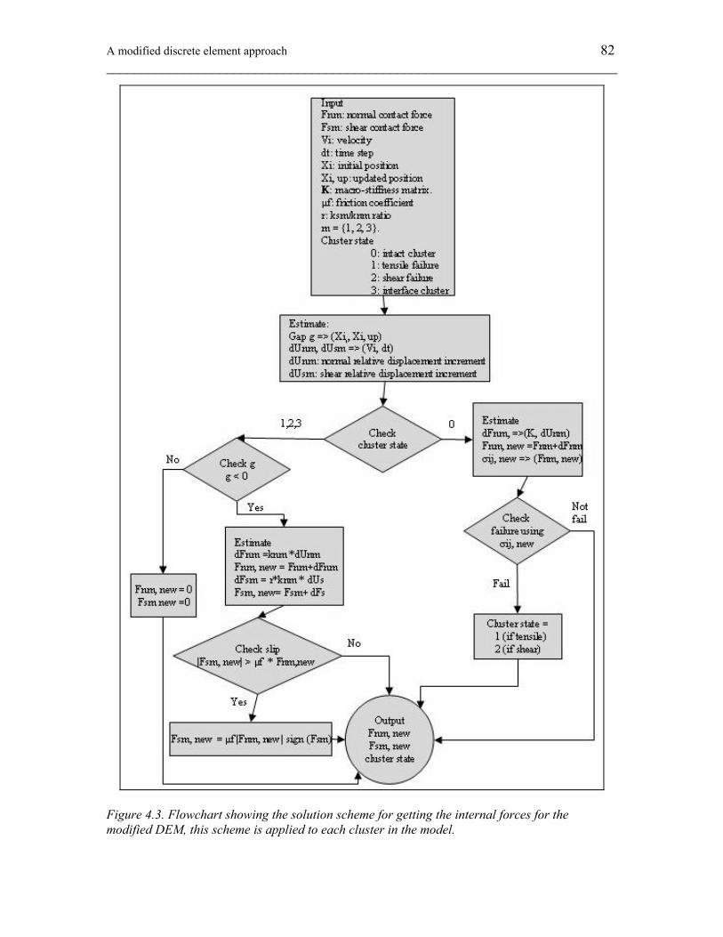
A modified discrete element approach 82 ________________________________________________________________________
Figure 4.3. Flowchart showing the solution scheme for getting the internal forces for the modified DEM, this scheme is applied to each cluster in the model.
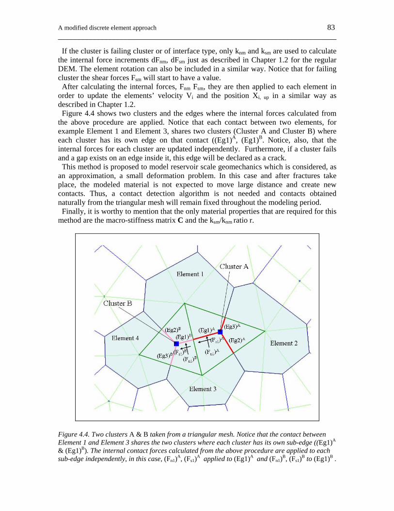
A modified discrete element approach 83 ________________________________________________________________________
If the cluster is failing cluster or of interface type, only knm and ksm are used to calculate the internal force increments dFnm, dFsm just as described in Chapter 1.2 for the regular DEM. The element rotation can also be included in a similar way. Notice that for failing cluster the shear forces Fsm will start to have a value. After calculating the internal forces, Fnm Fsm, they are then applied to each element in order to update the elements’ velocity Vi and the position Xi, up in a similar way as described in Chapter 1.2. Figure 4.4 shows two clusters and the edges where the internal forces calculated from the above procedure are applied. Notice that each contact between two elements, for example Element 1 and Element 3, shares two clusters (Cluster A and Cluster B) where each cluster has its own edge on that contact ((Eg1)A, (Eg1)B. Notice, also, that the internal forces for each cluster are updated independently. Furthermore, if a cluster fails and a gap exists on an edge inside it, this edge will be declared as a crack. This method is proposed to model reservoir scale geomechanics which is considered, as an approximation, a small deformation problem. In this case and after fractures take place, the modeled material is not expected to move large distance and create new contacts. Thus, a contact detection algorithm is not needed and contacts obtained naturally from the triangular mesh will remain fixed throughout the modeling period. Finally, it is worthy to mention that the only material properties that are required for this method are the macro-stiffness matrix C and the ksm/knm ratio r.
Figure 4.4. Two clusters A & B taken from a triangular mesh. Notice that the contact between Element 1 and Element 3 shares the two clusters where each cluster has its own sub-edge ((Eg1)A & (Eg1)B). The internal contact forces calculated from the above procedure are applied to each sub-edge independently, in this case, (Fn1)A, (Fs1)A applied to (Eg1)A and (Fn1)B, (Fs1)B to (Eg1)B .
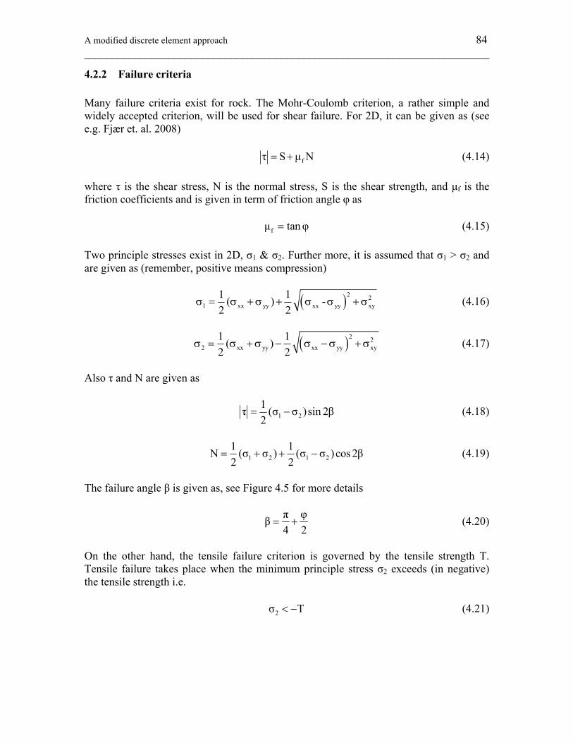
A modified discrete element approach 84 ________________________________________________________________________
4.2.2 Failure criteria Many failure criteria exist for rock. The Mohr-Coulomb criterion, a rather simple and widely accepted criterion, will be used for shear failure. For 2D, it can be given as (see e.g. Fjær et. al. 2008) fτ S μ N= + (4.14) where τ is the shear stress, N is the normal stress, S is the shear strength, and μf is the friction coefficients and is given in term of friction angle φ as fμ tanφ= (4.15) Two principle stresses exist in 2D, σ1 & σ2. Further more, it is assumed that σ1 > σ2 and are given as (remember, positive means compression)
( )2 21 xx yy xx yy xy
1 1( ) -2 2
σ = σ + σ + σ σ + σ (4.16)
( )2 22 xx yy xx yy xy
1 1( )2 2
σ = σ + σ − σ − σ + σ (4.17)
Also τ and N are given as
1 21τ (σ σ )sin 2β2
= − (4.18)
1 2 1 21 1N (σ σ ) (σ σ ) cos 2β2 2
= + + − (4.19)
The failure angle β is given as, see Figure 4.5 for more details
π φβ4 2
= + (4.20)
On the other hand, the tensile failure criterion is governed by the tensile strength T. Tensile failure takes place when the minimum principle stress σ2 exceeds (in negative) the tensile strength i.e. 2σ T< − (4.21)
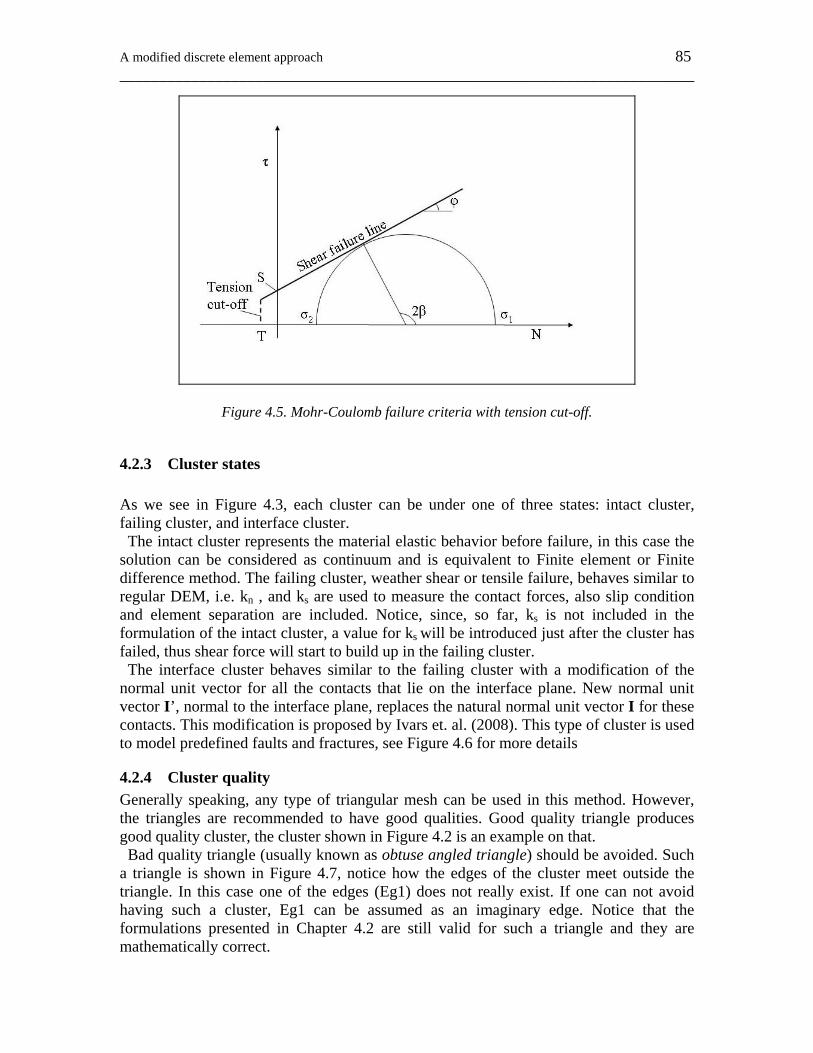
A modified discrete element approach 85 ________________________________________________________________________
Figure 4.5. Mohr-Coulomb failure criteria with tension cut-off.
4.2.3 Cluster states As we see in Figure 4.3, each cluster can be under one of three states: intact cluster, failing cluster, and interface cluster. The intact cluster represents the material elastic behavior before failure, in this case the solution can be considered as continuum and is equivalent to Finite element or Finite difference method. The failing cluster, weather shear or tensile failure, behaves similar to regular DEM, i.e. kn , and ks are used to measure the contact forces, also slip condition and element separation are included. Notice, since, so far, ks is not included in the formulation of the intact cluster, a value for ks will be introduced just after the cluster has failed, thus shear force will start to build up in the failing cluster. The interface cluster behaves similar to the failing cluster with a modification of the normal unit vector for all the contacts that lie on the interface plane. New normal unit vector I’, normal to the interface plane, replaces the natural normal unit vector I for these contacts. This modification is proposed by Ivars et. al. (2008). This type of cluster is used to model predefined faults and fractures, see Figure 4.6 for more details
4.2.4 Cluster quality Generally speaking, any type of triangular mesh can be used in this method. However, the triangles are recommended to have good qualities. Good quality triangle produces good quality cluster, the cluster shown in Figure 4.2 is an example on that. Bad quality triangle (usually known as obtuse angled triangle) should be avoided. Such a triangle is shown in Figure 4.7, notice how the edges of the cluster meet outside the triangle. In this case one of the edges (Eg1) does not really exist. If one can not avoid having such a cluster, Eg1 can be assumed as an imaginary edge. Notice that the formulations presented in Chapter 4.2 are still valid for such a triangle and they are mathematically correct.
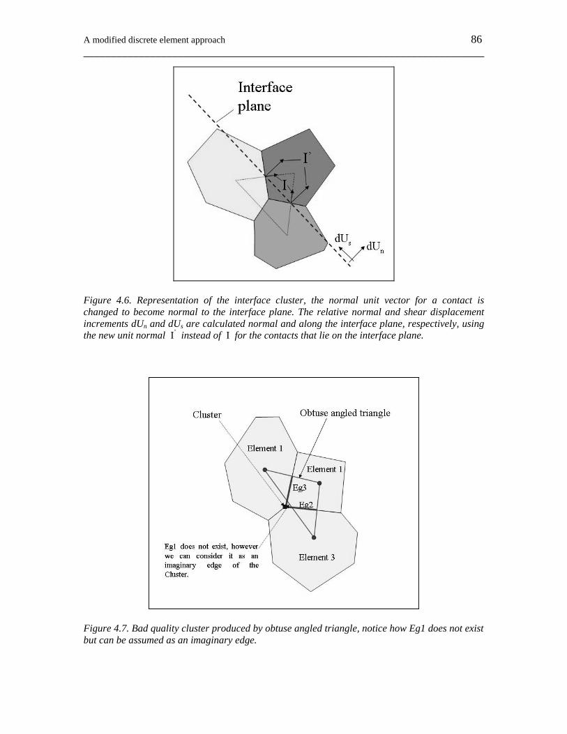
A modified discrete element approach 86 ________________________________________________________________________
Figure 4.6. Representation of the interface cluster, the normal unit vector for a contact is changed to become normal to the interface plane. The relative normal and shear displacement increments dUn and dUs are calculated normal and along the interface plane, respectively, using the new unit normal I’ instead of I for the contacts that lie on the interface plane.
Figure 4.7. Bad quality cluster produced by obtuse angled triangle, notice how Eg1 does not exist but can be assumed as an imaginary edge.
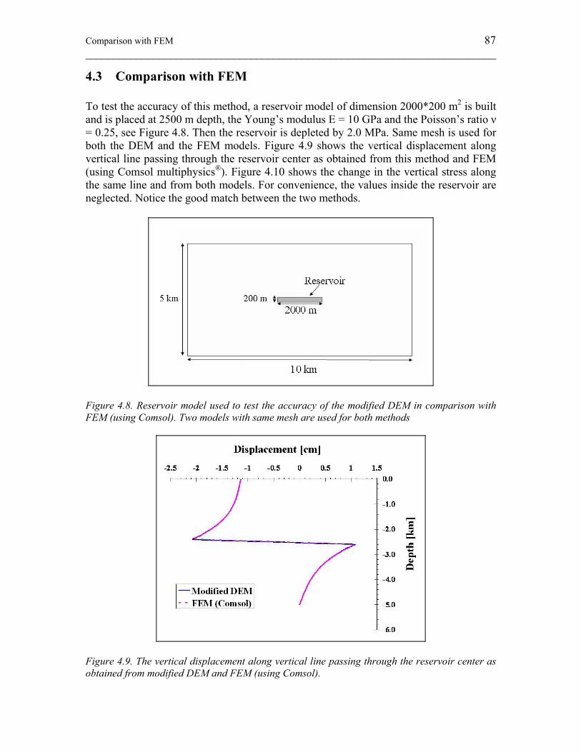
Comparison with FEM 87 ________________________________________________________________________
4.3 Comparison with FEM To test the accuracy of this method, a reservoir model of dimension 2000*200 m2 is built and is placed at 2500 m depth, the Young’s modulus E = 10 GPa and the Poisson’s ratio ν = 0.25, see Figure 4.8. Then the reservoir is depleted by 2.0 MPa. Same mesh is used for both the DEM and the FEM models. Figure 4.9 shows the vertical displacement along vertical line passing through the reservoir center as obtained from this method and FEM (using Comsol multiphysics®). Figure 4.10 shows the change in the vertical stress along the same line and from both models. For convenience, the values inside the reservoir are neglected. Notice the good match between the two methods.
Figure 4.8. Reservoir model used to test the accuracy of the modified DEM in comparison with FEM (using Comsol). Two models with same mesh are used for both methods
Figure 4.9. The vertical displacement along vertical line passing through the reservoir center as obtained from modified DEM and FEM (using Comsol).
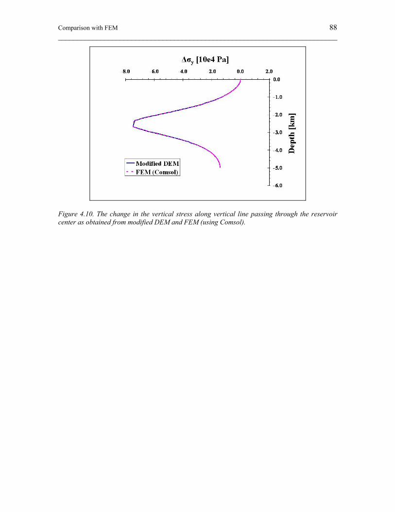
Comparison with FEM 88 ________________________________________________________________________
Figure 4.10. The change in the vertical stress along vertical line passing through the reservoir center as obtained from modified DEM and FEM (using Comsol).
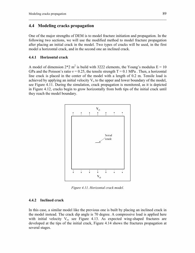
Modeling cracks propagation 89 ________________________________________________________________________
4.4 Modeling cracks propagation One of the major strengths of DEM is to model fracture initiation and propagation. In the following two sections, we will use the modified method to model fracture propagation after placing an initial crack in the model. Two types of cracks will be used, in the first model a horizontal crack, and in the second one an inclined crack.
4.4.1 Horizontal crack A model of dimension 2*2 m2 is build with 3222 elements, the Young’s modulus E = 10 GPa and the Poisson’s ratio ν = 0.25, the tensile strength T = 0.1 MPa . Then, a horizontal line crack is placed in the center of the model with a length of 0.2 m. Tensile load is achieved by applying an initial velocity Vo to the upper and lower boundary of the model, see Figure 4.11. During the simulation, crack propagation is monitored, as it is depicted in Figure 4.12, cracks begin to grow horizontally from both tips of the initial crack until they reach the model boundary.
Figure 4.11. Horizontal crack model.
4.4.2 Inclined crack In this case, a similar model like the previous one is built by placing an inclined crack in the model instead. The crack dip angle is 70 degree. A compressive load is applied here with initial velocity Vo, see Figure 4.13. As expected wing-shaped fractures are developed at the tips of the initial crack, Figure 4.14 shows the fractures propagation at several stages.
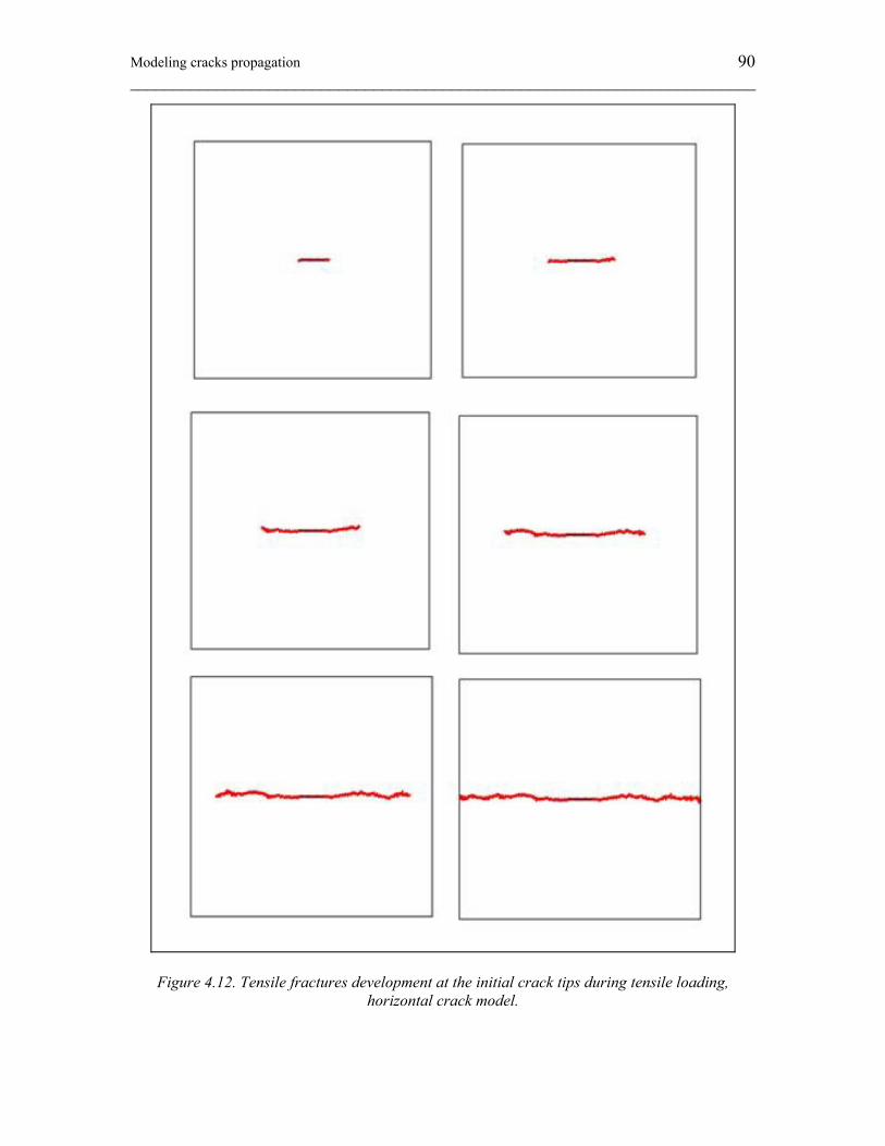
Modeling cracks propagation 90 ________________________________________________________________________
Figure 4.12. Tensile fractures development at the initial crack tips during tensile loading, horizontal crack model.
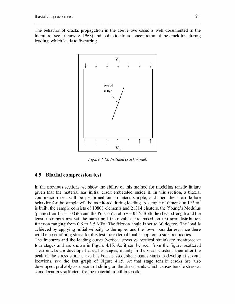
Biaxial compression test 91 ________________________________________________________________________
The behavior of cracks propagation in the above two cases is well documented in the literature (see Liebowitz, 1968) and is due to stress concentration at the crack tips during loading, which leads to fracturing.
Figure 4.13. Inclined crack model.
4.5 Biaxial compression test In the previous sections we show the ability of this method for modeling tensile failure given that the material has initial crack embedded inside it. In this section, a biaxial compression test will be performed on an intact sample, and then the shear failure behavior for the sample will be monitored during loading. A sample of dimension 1*2 m2 is built, the sample consists of 10808 elements and 21314 clusters, the Young’s Modulus (plane strain) E = 10 GPa and the Poisson’s ratio ν = 0.25. Both the shear strength and the tensile strength are set the same and their values are based on uniform distribution function ranging from 0.5 to 3.5 MPa. The friction angle is set to 30 degree. The load is achieved by applying initial velocity to the upper and the lower boundaries, since there will be no confining stress for this test, no external load is applied to side boundaries. The fractures and the loading curve (vertical stress vs. vertical strain) are monitored at four stages and are shown in Figure 4.15. As it can be seen from the figure, scattered shear cracks are developed at earlier stages, mainly in the weak clusters, then after the peak of the stress strain curve has been passed, shear bands starts to develop at several locations, see the last graph of Figure 4.15. At that stage tensile cracks are also developed, probably as a result of sliding on the shear bands which causes tensile stress at some locations sufficient for the material to fail in tensile.
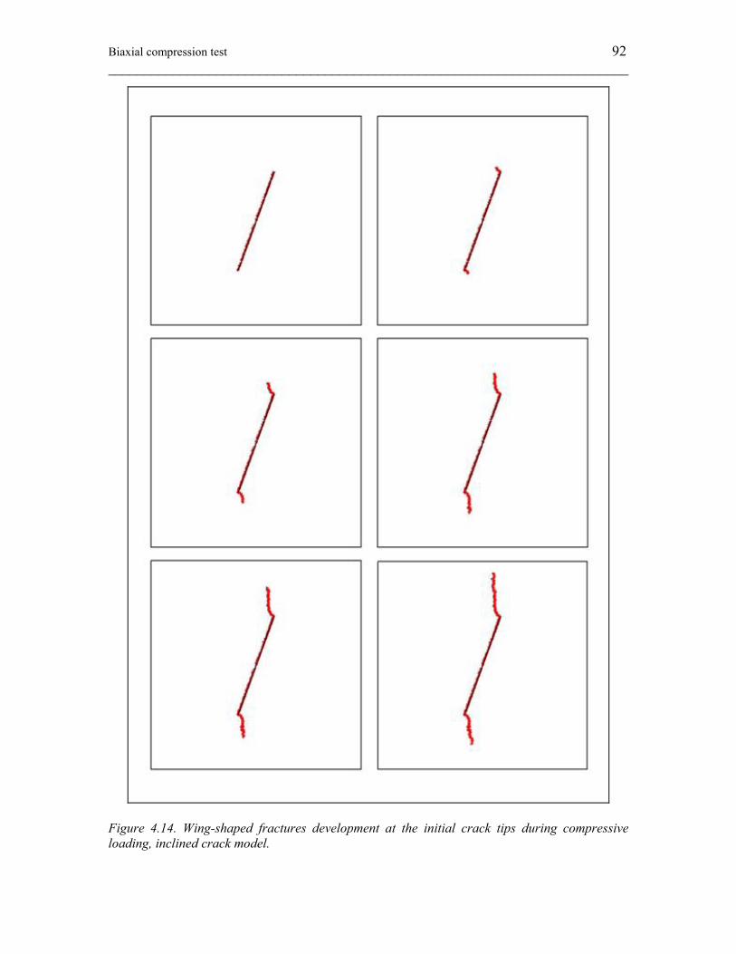
Biaxial compression test 92 ________________________________________________________________________
Figure 4.14. Wing-shaped fractures development at the initial crack tips during compressive loading, inclined crack model.
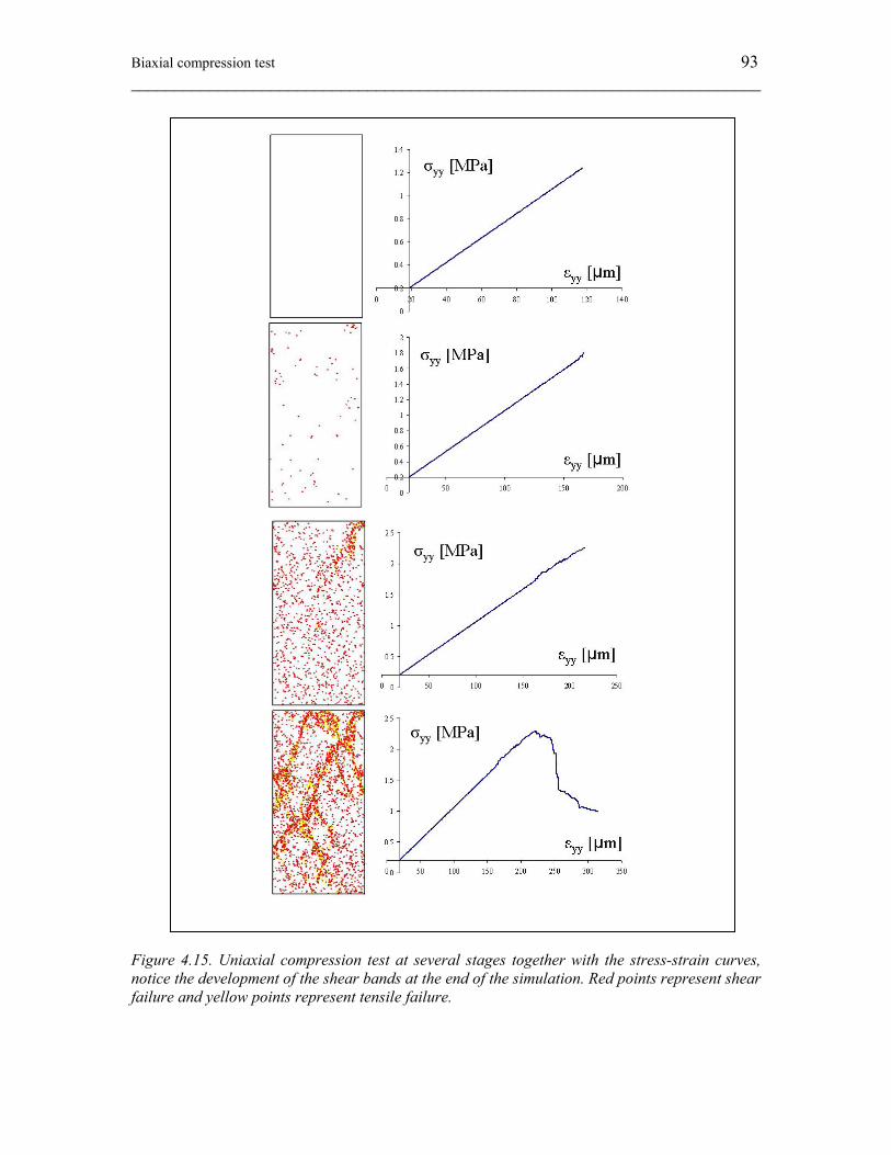
Biaxial compression test 93 ________________________________________________________________________
Figure 4.15. Uniaxial compression test at several stages together with the stress-strain curves, notice the development of the shear bands at the end of the simulation. Red points represent shear failure and yellow points represent tensile failure.
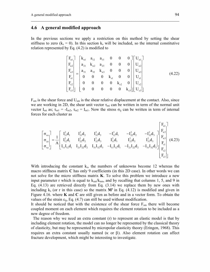
A general modified approach 94 ________________________________________________________________________
4.6 A general modified approach In the previous sections we apply a restriction on this method by setting the shear stiffness to zero (ks = 0). In this section ks will be included, so the internal constitutive relation represented by Eq. (4.2) is modified to
n1 n1 12 13 n1
n2 21 n2 23 n2
n3 31 32 n3 n3
s1 s1 s1
s2 s2 s2
s3 s3 s3
F k a a 0 0 0 UF a k a 0 0 0 UF a a k 0 0 0 UF 0 0 0 k 0 0 UF 0 0 0 0 k 0 UF 0 0 0 0 0 k U
⎡ ⎤ ⎡ ⎤ ⎡ ⎤⎢ ⎥ ⎢ ⎥ ⎢ ⎥⎢ ⎥ ⎢ ⎥ ⎢ ⎥⎢ ⎥ ⎢ ⎥ ⎢ ⎥
=⎢ ⎥ ⎢ ⎥ ⎢ ⎥⎢ ⎥ ⎢ ⎥ ⎢ ⎥⎢ ⎥ ⎢ ⎥ ⎢ ⎥⎢ ⎥ ⎢ ⎥ ⎢ ⎥⎢ ⎥ ⎢ ⎥ ⎢ ⎥⎣ ⎦ ⎣ ⎦ ⎣ ⎦
(4.22)
Fsm is the shear force and Usm is the shear relative displacement at the contact. Also, since we are working in 2D, the shear unit vector τmi can be written in term of the normal unit vector Imi as; τm1 = -Im2, τm2 = Im1. Now the stress σij can be written in term of internal forces for each cluster as
n1
n 22 2 2 2 2 2xx 11 1 21 2 31 3 12 1 22 2 32 3
n32 2 2 2 2 2yy 12 1 22 2 32 3 11 1 21 2 31 3
s1xy 11 12 1 21 22 2 31 32 3 11 12 1 21 22 2 31 32 3
s2
s3
FF
σ I d I d I d I d I d I dF1σ I d I d I d I d I d I dFA
σ I I d I I d I I d I I d I I d I I dFF
⎡ ⎤⎢ ⎥⎢ ⎥⎡ ⎤⎡ ⎤ − − −⎢ ⎥⎢ ⎥⎢ ⎥ = ⎢ ⎥⎢ ⎥⎢ ⎥⎢ ⎥⎢ ⎥⎢ ⎥ − − −⎣ ⎦ ⎣ ⎦ ⎢ ⎥⎢ ⎥⎢ ⎥⎣ ⎦
(4.23)
With introducing the constant ks, the numbers of unknowns become 12 whereas the macro stiffness matrix C has only 9 coefficients (in this 2D case). In other words we can not solve for the micro stiffness matrix K. To solve this problem we introduce a new input parameter r which is equal to ksm/knm, and by recalling that columns 1, 5, and 9 in Eq. (4.13) are retrieved directly from Eq. (3.14) we replace them by new ones with including ks (or r in this case) so the matrix M' in Eq. (4.12) is modified and given in Figure 4.16. where K and C are still given as before and in a vector form. To obtain the values of the strain εij, Eq. (4.7) can still be used without modification. It should be noticed that with the existence of the shear force Fsm there will become coupled moment on each element which requires the element rotation to be included as a new degree of freedom. The reason why we need an extra constant (r) to represent an elastic model is that by including element rotation, the model can no longer be represented by the classical theory of elasticity, but may be represented by micropolar elasticity theory (Eringen, 1968). This requires an extra constant usually named (κ or β). Also element rotation can affect fracture development, which might be interesting to investigate.
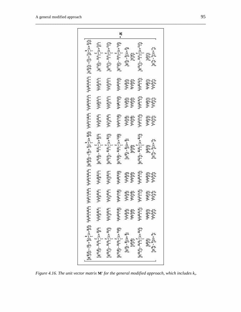
A general modified approach 95 ________________________________________________________________________
Figure 4.16. The unit vector matrix M' for the general modified approach, which includes ks.
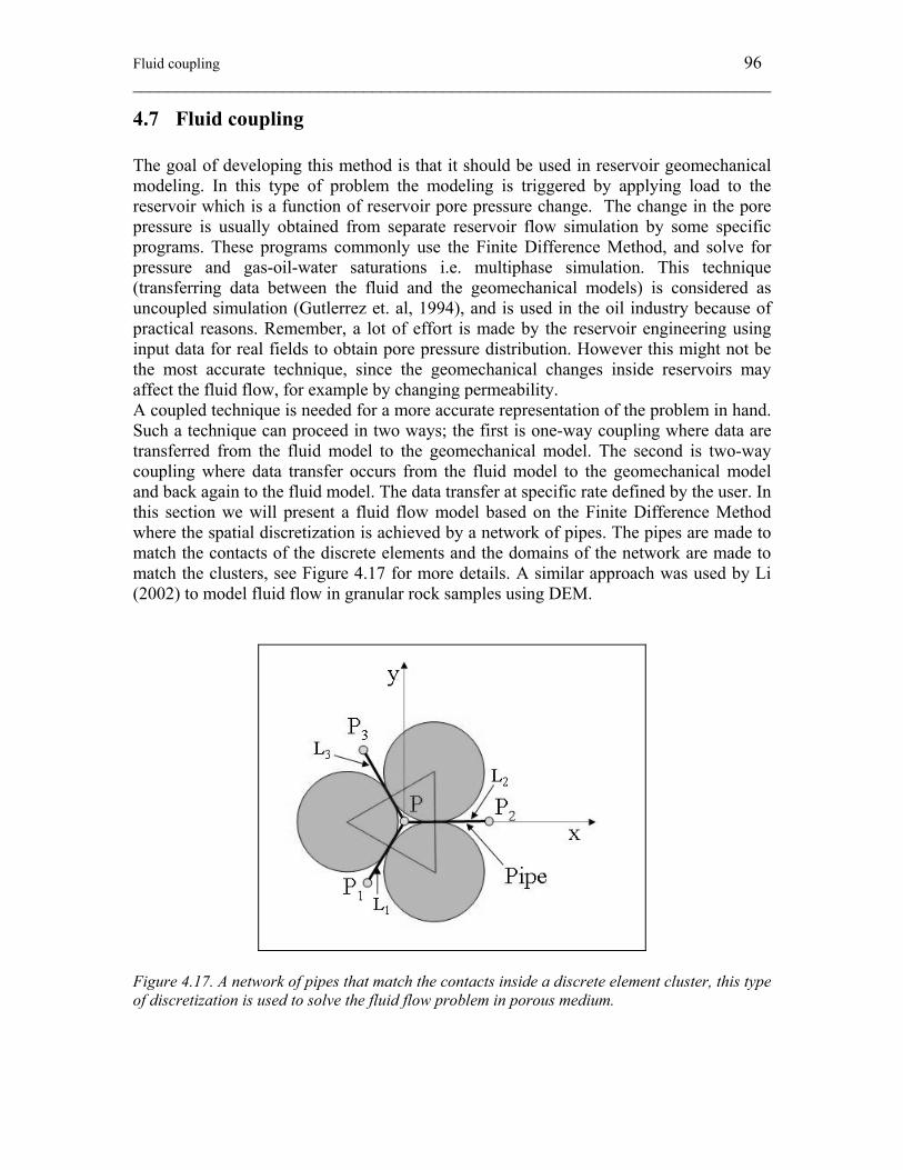
Fluid coupling 96 ________________________________________________________________________
4.7 Fluid coupling The goal of developing this method is that it should be used in reservoir geomechanical modeling. In this type of problem the modeling is triggered by applying load to the reservoir which is a function of reservoir pore pressure change. The change in the pore pressure is usually obtained from separate reservoir flow simulation by some specific programs. These programs commonly use the Finite Difference Method, and solve for pressure and gas-oil-water saturations i.e. multiphase simulation. This technique (transferring data between the fluid and the geomechanical models) is considered as uncoupled simulation (Gutlerrez et. al, 1994), and is used in the oil industry because of practical reasons. Remember, a lot of effort is made by the reservoir engineering using input data for real fields to obtain pore pressure distribution. However this might not be the most accurate technique, since the geomechanical changes inside reservoirs may affect the fluid flow, for example by changing permeability. A coupled technique is needed for a more accurate representation of the problem in hand. Such a technique can proceed in two ways; the first is one-way coupling where data are transferred from the fluid model to the geomechanical model. The second is two-way coupling where data transfer occurs from the fluid model to the geomechanical model and back again to the fluid model. The data transfer at specific rate defined by the user. In this section we will present a fluid flow model based on the Finite Difference Method where the spatial discretization is achieved by a network of pipes. The pipes are made to match the contacts of the discrete elements and the domains of the network are made to match the clusters, see Figure 4.17 for more details. A similar approach was used by Li (2002) to model fluid flow in granular rock samples using DEM.
Figure 4.17. A network of pipes that match the contacts inside a discrete element cluster, this type of discretization is used to solve the fluid flow problem in porous medium.
Fluid coupling 97 ________________________________________________________________________
As shown in Figure 4.17 each fluid domain has three pipes and the flow rate q in each pipe can be given using Darcy’s law as follows
ii i
i
kq (P P )L μ
= − (4.24)
where ki is the permeability of the pipe, Li is the pipe length, μ is the fluid viscosity, and P, Pi are the pressures of the domain of concern and the other connected domains, respectively. Now we can write an expression for Pi based on Taylor’s expansion as follows
2 2 2
2 2i i i i i i i2 2
i i i 1
1 P 1 P PP P x y x y O(x , y )2 x 2 y x y
∂ ∂ ∂= + + + +
∂ ∂ ∂ ∂ (4.25)
where O(xi,yi) is a first order error if a random mesh is used , and this error will be of third order if a uniform mesh is used like that shown in Figure 4.19a. However, for random mesh and as the mesh resolution increases the error terms may cancel each other and the total error becomes small. The flow rates qi to the domain will result in a fluid volume change in that domain which can be given as
f1 2 3
f
ΔV q q qΔt
= + + (4.26)
Δtf is a fluid time step, also the fluid compressibility cf can be given as
ff
f
V1cV P
∂= −
∂ (4.27)
The fluid volume Vf = ΦA, where Φ is the porosity and A is the domain area (since we are working in 2D). Also we define xi = Ii1Li and yi = Ii2Li, where Ii is the unit vector and Li is the length of the pipe (Ii1 = cosθi, Ii2 = sinθi). Then by using the approximation Δ ~ ∂ and the above equations one may write
2 22 2 2 2 2
f 11 1 1 21 2 2 31 3 3 12 1 1 22 2 22 2
2232 3 3 11 12 1 1 21 22 2 2 31 32 3 3
P 1 P 1 PAΦμc (I L k I L k I L k ) (I L k I L kt 2 x 2 y
PI L k ) (I I L k I I L k I I L k )x y
∂ ∂ ∂= + + + +
∂ ∂ ∂
∂+ + + +
∂ ∂
(4.28)
Recall that the partial differential equation for fluid flow in porous media may be given as
2 2 2
f xx yy xy2 2
P P P PΦμc k k kt x y x y
∂ ∂ ∂ ∂= + +
∂ ∂ ∂ ∂ ∂ (4.29)
Fluid coupling 98 ________________________________________________________________________
where kij is the permeability tensor for the porous media. So by comparing Eq. (4.28) and Eq. (4.29), one can obtain a relation between the permeability tensor kij and the permeability of the pipes for each cluster in a matrix form as follows
2 2 2xx 11 1 21 2 31 3 1
2 2 2yy 12 1 22 2 32 3 2
xy 11 12 1 21 22 2 31 32 3 3
k I L I L I L k1k I L I L I L k
2Ak 2I I L 2I I L 2I I L k
⎡ ⎤⎡ ⎤ ⎡ ⎤⎢ ⎥⎢ ⎥ ⎢ ⎥= ⎢ ⎥⎢ ⎥ ⎢ ⎥⎢ ⎥⎢ ⎥ ⎢ ⎥⎣ ⎦⎣ ⎦ ⎣ ⎦
(4.30)
4.7.1 Solution procedure The solution starts by finding the pipe permeability ki for each cluster using Eq. (4.30), one has to notice that each pipe shares two clusters (back to Figure 4.4) so the total permeability of a specific pipe is actually a contribution of two sub-pipes connected in series. After that, Eqs. (4.24) & (4.26) are used to calculate the change in the fluid volume for each cluster, and then the pore pressure is updated based on Eq. (4.27) as follows
new old ff
1P P ΔVAΦc
= + (4.31)
This is for one-way coupling, if two-way coupling is needed then Eq. (4.31) becomes
new old f vf
1P P (ΔV AΔε )AΦc
= + − (4.32)
Where Δεv is the change in volumetric strain as obtain from the geomechanical model during one fluid cycle (i.e. Δtf). Since the fluid pressure front is considered slow relative to the stress (wave) front in the rock, for each fluid time step (Δtf) the geomechanical model is run to equilibrium before starting another fluid time step. The geomechanical model uses the pressure distribution obtained from the fluid flow model as external load. Also, because this is an explicit solution, the smaller Δtf the more accurate the solution is, and there will be a restriction on the maximum value of Δtf to give a stable solution.
4.7.2 Restriction on the mesh quality As we have said before, a random (or non-uniform) mesh is preferable in this technique to produce a random distribution of discrete elements. Random mesh generation codes are usually used to build the models. However, the resulted mesh does not necessary have high quality. To give an example, Figure 4.18 shows two triangles which are taken from a random mesh. The triangle to the left has “good” quality and to right has “poor” one. To construct the pipes network for fluid flow, lines start from the middle of the triangle edges and perpendicular to those edges are created. Where these lines meet represents the fluid domain. Unlike the left triangle, the right triangle has its pipes met outside it. For such a case, one of the pipes’ permeability ki obtained from Eq. (4.30) will have negative
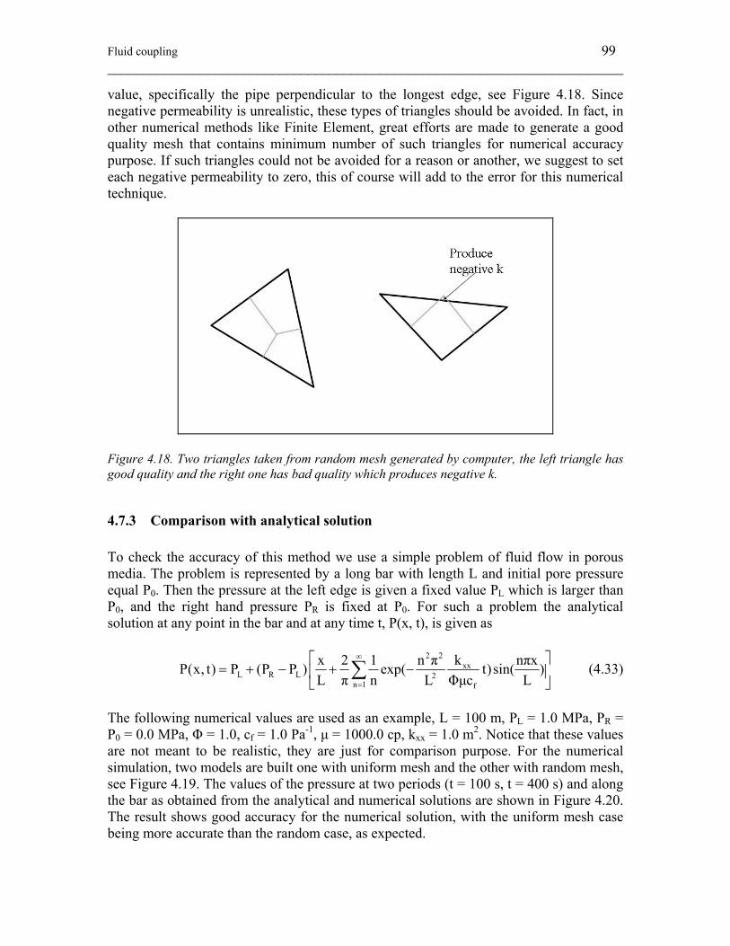
Fluid coupling 99 ________________________________________________________________________
value, specifically the pipe perpendicular to the longest edge, see Figure 4.18. Since negative permeability is unrealistic, these types of triangles should be avoided. In fact, in other numerical methods like Finite Element, great efforts are made to generate a good quality mesh that contains minimum number of such triangles for numerical accuracy purpose. If such triangles could not be avoided for a reason or another, we suggest to set each negative permeability to zero, this of course will add to the error for this numerical technique.
Figure 4.18. Two triangles taken from random mesh generated by computer, the left triangle has good quality and the right one has bad quality which produces negative k.
4.7.3 Comparison with analytical solution To check the accuracy of this method we use a simple problem of fluid flow in porous media. The problem is represented by a long bar with length L and initial pore pressure equal P0. Then the pressure at the left edge is given a fixed value PL which is larger than P0, and the right hand pressure PR is fixed at P0. For such a problem the analytical solution at any point in the bar and at any time t, P(x, t), is given as
2 2
xxL R L 2
n 1 f
kx 2 1 n π nπxP(x, t) P (P P ) exp( t)sin( )L π n L Φμc L
∞
=
⎡ ⎤= + − + −⎢ ⎥
⎣ ⎦∑ (4.33)
The following numerical values are used as an example, L = 100 m, PL = 1.0 MPa, PR = P0 = 0.0 MPa, Φ = 1.0, cf = 1.0 Pa-1, μ = 1000.0 cp, kxx = 1.0 m2. Notice that these values are not meant to be realistic, they are just for comparison purpose. For the numerical simulation, two models are built one with uniform mesh and the other with random mesh, see Figure 4.19. The values of the pressure at two periods (t = 100 s, t = 400 s) and along the bar as obtained from the analytical and numerical solutions are shown in Figure 4.20. The result shows good accuracy for the numerical solution, with the uniform mesh case being more accurate than the random case, as expected.
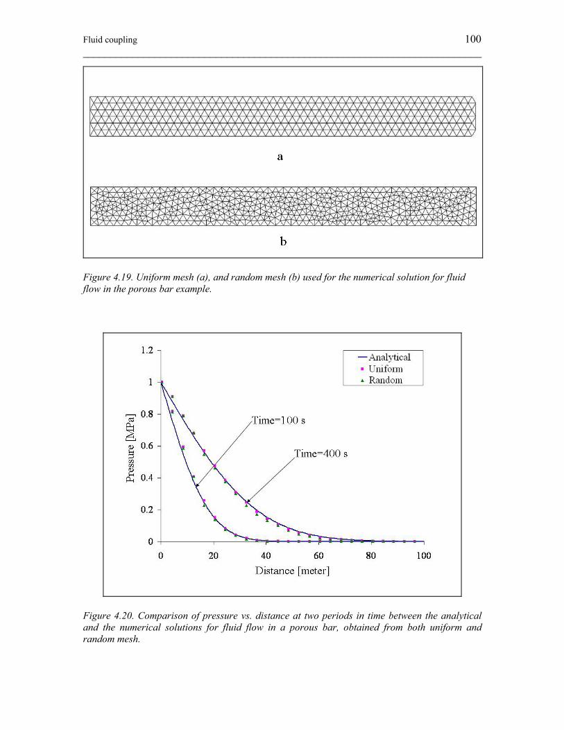
Fluid coupling 100 ________________________________________________________________________
Figure 4.19. Uniform mesh (a), and random mesh (b) used for the numerical solution for fluid flow in the porous bar example.
Figure 4.20. Comparison of pressure vs. distance at two periods in time between the analytical and the numerical solutions for fluid flow in a porous bar, obtained from both uniform and random mesh.
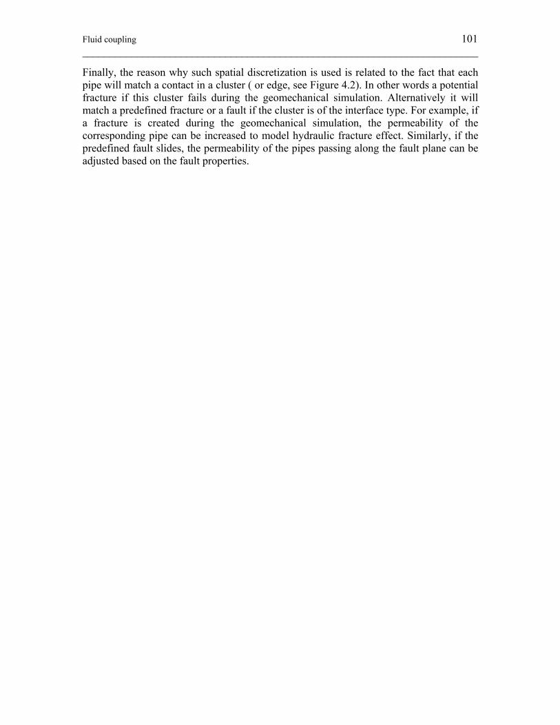
Fluid coupling 101 ________________________________________________________________________
Finally, the reason why such spatial discretization is used is related to the fact that each pipe will match a contact in a cluster ( or edge, see Figure 4.2). In other words a potential fracture if this cluster fails during the geomechanical simulation. Alternatively it will match a predefined fracture or a fault if the cluster is of the interface type. For example, if a fracture is created during the geomechanical simulation, the permeability of the corresponding pipe can be increased to model hydraulic fracture effect. Similarly, if the predefined fault slides, the permeability of the pipes passing along the fault plane can be adjusted based on the fault properties.

102 ________________________________________________________________________
Chapter 5: Reservoir geomechanical modeling 103 ________________________________________________________________________
5 Reservoir geomechanical modeling for some North Sea cases: A comparison to 4D seismics.
* Part of this chapter is presented and published in the Extended Abstract of EAGE Conference, Rome, 2008.
5.1 Introduction The modified discrete element approach presented in Chapter 4 will be used in this chapter to model reservoir geomechanical response to pressure change. Some real geological sections for hydrocarbon reservoirs taken from the North Sea will be used for that purpose. In the first section, the stress path coefficient presented in Chapter 1 is used to investigate the possibility of creating vertical or horizontal fractures during fluid injection. A numerical test on an elliptical reservoir will be provided as an example. Then a 2D synthetic section for the Gullfaks field in the North Sea is built, and fluid flow together with geomechanical modeling is implemented on this section. The modeling is triggered by injecting fluid into a horizontal well passing through the reservoir using the fluid-coupling approach described in Chapter 4. Because of the uncertainty in reservoir properties and other given data, two scenarios will be studied, the first one with low horizontal effective stress and the second one with low vertical effective stress. In both cases fracture development will be monitored. A time-lapse seismics cross section for Gullfaks field will be shown and compared to the above two scenarios based on an interpretation by Landrø et. al. (2001). Next, the stress path coefficient will be used to investigate the possibility of rock failure in hydrocarbon reservoirs during depletion i.e. pore pressure reduction. The most likely type of failure in this case is shear failure. After that, fault reactivation possibilities during reservoir depletion on two real reservoirs’ sections will be studied. The sections are taken from Elgin-Franklin gas reservoir provided by (Total E&P UK Ltd.).The study will focus on how faults may slide and how that can affect the stress field around the reservoir. The effects of the reservoir geometry including the reservoir compartments will also be studied. If such effects can be detected using time lapse seismic, then certain measure may be taken to avoid failure in well casing as a result of fault sliding, also this may help us to track which compartment is producing and which is not if the saturation change is not sufficient to give such information. It is still early, however, to say that fault reactivation, if it happens, may be detected by time lapse seismic. Finally, a time-lapse seismic cross section for Elgin-Franklin reservoir will be shown and compared to the geomechanical model. In the last section, we will show how the fractures that are developed inside the reservoir during fluid change may be converted to velocity change which in turn creates velocity models that can be used in seismic modeling for time-lapse seismics studies. Rock
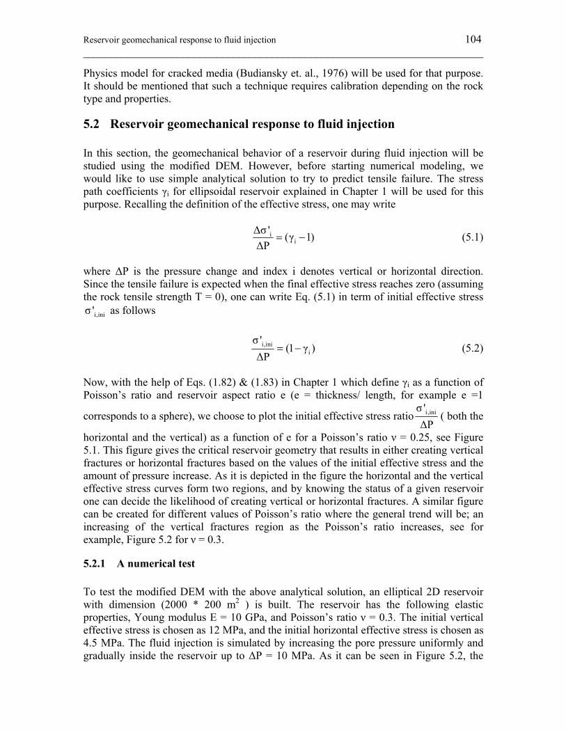
Reservoir geomechanical response to fluid injection 104 ________________________________________________________________________
Physics model for cracked media (Budiansky et. al., 1976) will be used for that purpose. It should be mentioned that such a technique requires calibration depending on the rock type and properties.
5.2 Reservoir geomechanical response to fluid injection In this section, the geomechanical behavior of a reservoir during fluid injection will be studied using the modified DEM. However, before starting numerical modeling, we would like to use simple analytical solution to try to predict tensile failure. The stress path coefficients γi for ellipsoidal reservoir explained in Chapter 1 will be used for this purpose. Recalling the definition of the effective stress, one may write
ii
Δσ ' (γ 1)ΔP
= − (5.1)
where ΔP is the pressure change and index i denotes vertical or horizontal direction. Since the tensile failure is expected when the final effective stress reaches zero (assuming the rock tensile strength T = 0), one can write Eq. (5.1) in term of initial effective stress
i,iniσ ' as follows
i,inii
σ '(1 γ )
ΔP= − (5.2)
Now, with the help of Eqs. (1.82) & (1.83) in Chapter 1 which define γi as a function of Poisson’s ratio and reservoir aspect ratio e (e = thickness/ length, for example e =1
corresponds to a sphere), we choose to plot the initial effective stress ratio i,iniσ 'ΔP
( both the
horizontal and the vertical) as a function of e for a Poisson’s ratio ν = 0.25, see Figure 5.1. This figure gives the critical reservoir geometry that results in either creating vertical fractures or horizontal fractures based on the values of the initial effective stress and the amount of pressure increase. As it is depicted in the figure the horizontal and the vertical effective stress curves form two regions, and by knowing the status of a given reservoir one can decide the likelihood of creating vertical or horizontal fractures. A similar figure can be created for different values of Poisson’s ratio where the general trend will be; an increasing of the vertical fractures region as the Poisson’s ratio increases, see for example, Figure 5.2 for ν = 0.3.
5.2.1 A numerical test To test the modified DEM with the above analytical solution, an elliptical 2D reservoir with dimension (2000 * 200 m2 ) is built. The reservoir has the following elastic properties, Young modulus E = 10 GPa, and Poisson’s ratio ν = 0.3. The initial vertical effective stress is chosen as 12 MPa, and the initial horizontal effective stress is chosen as 4.5 MPa. The fluid injection is simulated by increasing the pore pressure uniformly and gradually inside the reservoir up to ΔP = 10 MPa. As it can be seen in Figure 5.2, the
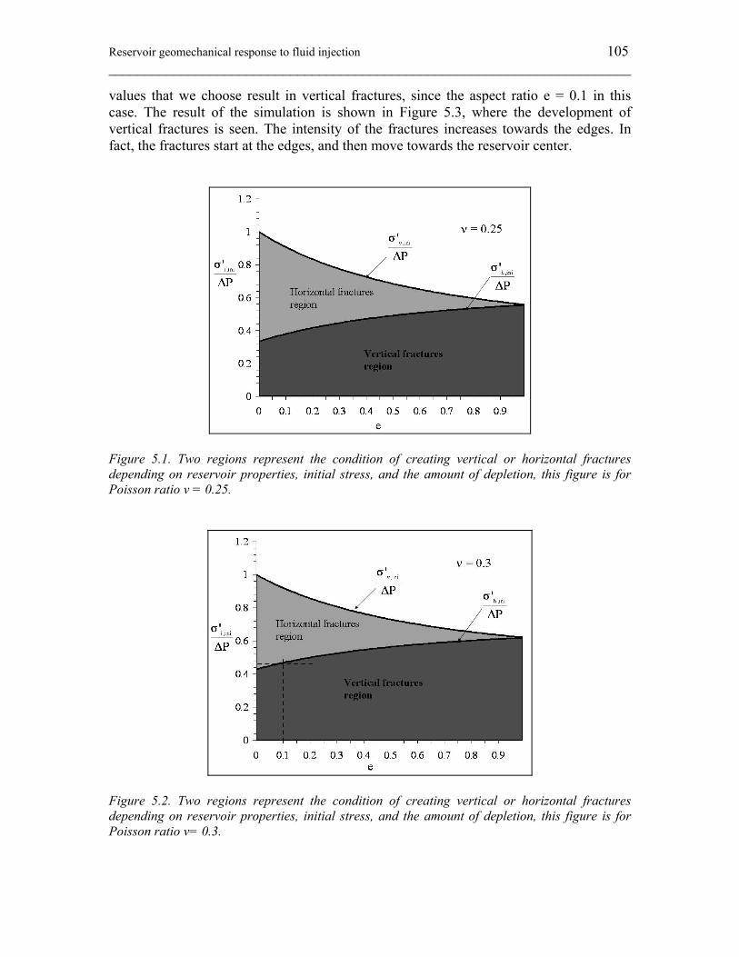
Reservoir geomechanical response to fluid injection 105 ________________________________________________________________________
values that we choose result in vertical fractures, since the aspect ratio e = 0.1 in this case. The result of the simulation is shown in Figure 5.3, where the development of vertical fractures is seen. The intensity of the fractures increases towards the edges. In fact, the fractures start at the edges, and then move towards the reservoir center.
Figure 5.1. Two regions represent the condition of creating vertical or horizontal fractures depending on reservoir properties, initial stress, and the amount of depletion, this figure is for Poisson ratio ν = 0.25.
Figure 5.2. Two regions represent the condition of creating vertical or horizontal fractures depending on reservoir properties, initial stress, and the amount of depletion, this figure is for Poisson ratio ν= 0.3.
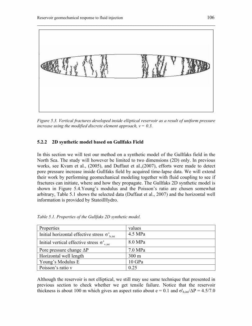
Reservoir geomechanical response to fluid injection 106 ________________________________________________________________________
Figure 5.3. Vertical fractures developed inside elliptical reservoir as a result of uniform pressure increase using the modified discrete element approach, ν = 0.3.
5.2.2 2D synthetic model based on Gullfaks Field In this section we will test our method on a synthetic model of the Gullfaks field in the North Sea. The study will however be limited to two dimensions (2D) only. In previous works, see Kvam et al., (2005), and Duffaut et al.,(2007), efforts were made to detect pore pressure increase inside Gullfaks field by acquired time-lapse data. We will extend their work by performing geomechanical modeling together with fluid coupling to see if fractures can initiate, where and how they propagate. The Gullfaks 2D synthetic model is shown in Figure 5.4.Young’s modulus and the Poisson’s ratio are chosen somewhat arbitrary, Table 5.1 shows the selected data (Duffaut et al., 2007) and the horizontal well information is provided by StatoilHydro. Table 5.1. Properties of the Gullfaks 2D synthetic model. Properties values Initial horizontal effective stress h,iniσ ' 4.5 MPa
Initial vertical effective stress v,iniσ ' 8.0 MPa Pore pressure change ΔP 7.0 MPa Horizontal well length 300 m Young’s Modulus E 10 GPa Poisson’s ratio ν 0.25
Although the reservoir is not elliptical, we still may use same technique that presented in previous section to check whether we get tensile failure. Notice that the reservoir thickness is about 100 m which gives an aspect ratio about e = 0.1 and σ'h,ini/ΔP = 4.5/7.0
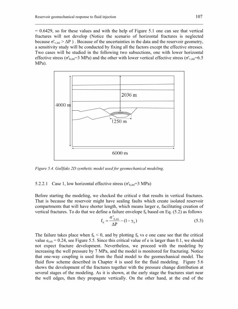
Reservoir geomechanical response to fluid injection 107 ________________________________________________________________________
= 0.6429, so for these values and with the help of Figure 5.1 one can see that vertical fractures will not develop (Notice the scenario of horizontal fractures is neglected because σ'v,ini > ΔP ) . Because of the uncertainties in the data and the reservoir geometry, a sensitivity study will be conducted by fixing all the factors except the effective stresses. Two cases will be studied in the following two subsections, one with lower horizontal effective stress (σ'h,ini=3 MPa) and the other with lower vertical effective stress (σ'v,ini=6.5 MPa).
Figure 5.4. Gullfaks 2D synthetic model used for geomechanical modeling.
5.2.2.1 Case 1, low horizontal effective stress (σ'h,ini=3 MPa) Before starting the modeling, we checked the critical e that results in vertical fractures. That is because the reservoir might have sealing faults which create isolated reservoir compartments that will have shorter length, which means larger e, facilitating creation of vertical fractures. To do that we define a failure envelope fh based on Eq. (5.2) as follows
h,inih h
σ 'f (1 γ )
ΔP= − − (5.3)
The failure takes place when fh < 0, and by plotting fh vs e one cane see that the critical value ecrit = 0.24, see Figure 5.5. Since this critical value of e is larger than 0.1, we should not expect fracture development. Nevertheless, we proceed with the modeling by increasing the well pressure by 7 MPa, and the model is monitored for fracturing. Notice that one-way coupling is used from the fluid model to the geomechanical model. The fluid flow scheme described in Chapter 4 is used for the fluid modeling. Figure 5.6 shows the development of the fractures together with the pressure change distribution at several stages of the modeling. As it is shown, at the early stage the fractures start near the well edges, then they propagate vertically. On the other hand, at the end of the
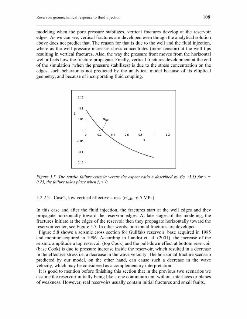
Reservoir geomechanical response to fluid injection 108 ________________________________________________________________________
modeling when the pore pressure stabilizes, vertical fractures develop at the reservoir edges. As we can see, vertical fractures are developed even though the analytical solution above does not predict that. The reason for that is due to the well and the fluid injection, where as the well pressure increases stress concentrates (more tension) at the well tips resulting in vertical fractures. Also, the way the pressure front moves from the horizontal well affects how the fracture propagate. Finally, vertical fractures development at the end of the simulation (when the pressure stabilizes) is due to the stress concentration on the edges, such behavior is not predicted by the analytical model because of its elliptical geometry, and because of incorporating fluid coupling.
Figure 5.5. The tensile failure criteria versus the aspect ratio e described by Eq. (5.3) for ν = 0.25, the failure takes place when fh < 0.
5.2.2.2 Case2, low vertical effective stress (σ'v,ini=6.5 MPa). In this case and after the fluid injection, the fractures start at the well edges and they propagate horizontally toward the reservoir edges. At late stages of the modeling, the fractures initiate at the edges of the reservoir then they propagate horizontally toward the reservoir center, see Figure 5.7. In other words, horizontal fractures are developed. Figure 5.8 shows a seismic cross section for Gullfaks reservoir, base acquired in 1985 and monitor acquired in 1996. According to Landrø et. al. (2001), the increase of the seismic amplitude a top reservoir (top Cook) and the pull-down effect at bottom reservoir (base Cook) is due to pressure increase inside the reservoir, which resulted in a decrease in the effective stress i.e. a decrease in the wave velocity. The horizontal fracture scenario predicted by our model, on the other hand, can cause such a decrease in the wave velocity, which may be considered as a complementary interpretation. It is good to mention before finishing this section that in the previous two scenarios we assume the reservoir initially being like a one continuum unit without interfaces or planes of weakness. However, real reservoirs usually contain initial fractures and small faults,
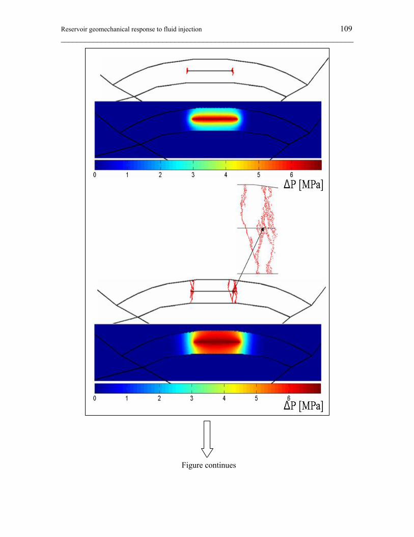
Reservoir geomechanical response to fluid injection 109 ________________________________________________________________________
Figure continues
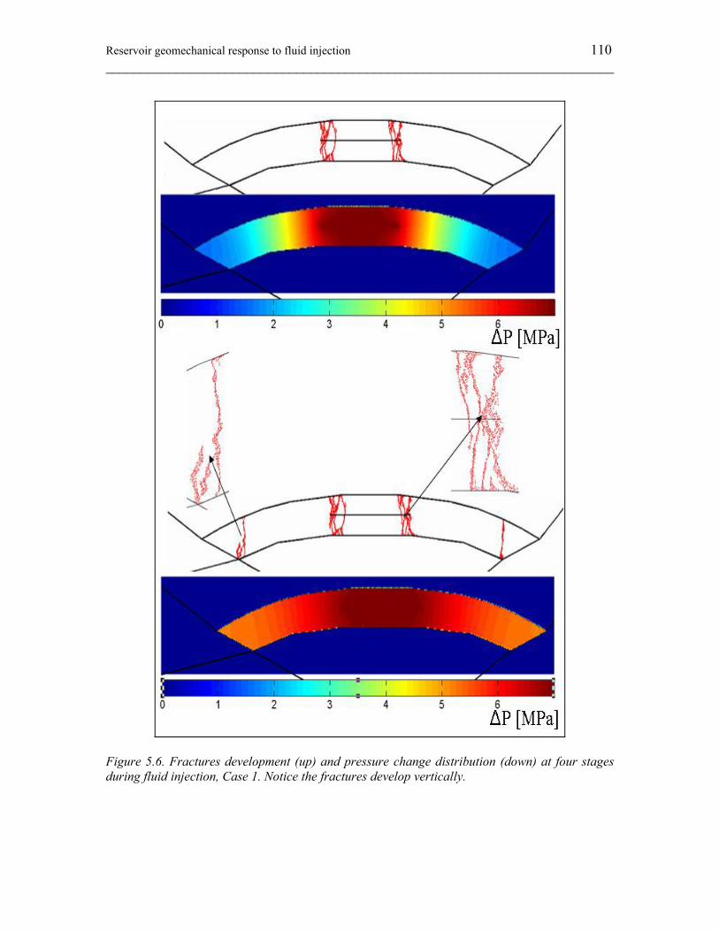
Reservoir geomechanical response to fluid injection 110 ________________________________________________________________________
Figure 5.6. Fractures development (up) and pressure change distribution (down) at four stages during fluid injection, Case 1. Notice the fractures develop vertically.
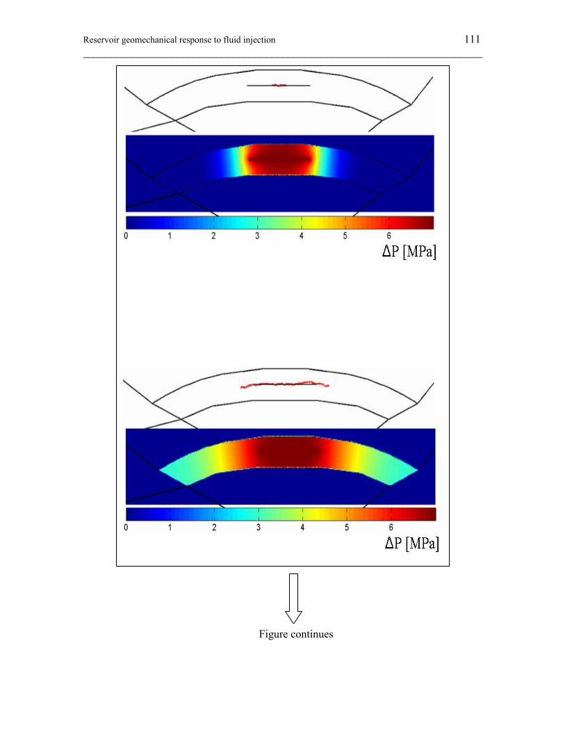
Reservoir geomechanical response to fluid injection 111 ________________________________________________________________________
Figure continues
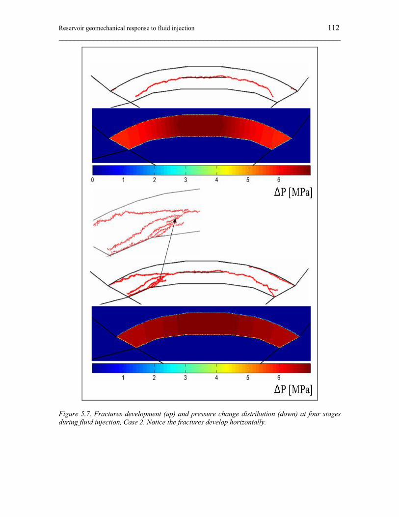
Reservoir geomechanical response to fluid injection 112 ________________________________________________________________________
Figure 5.7. Fractures development (up) and pressure change distribution (down) at four stages during fluid injection, Case 2. Notice the fractures develop horizontally.
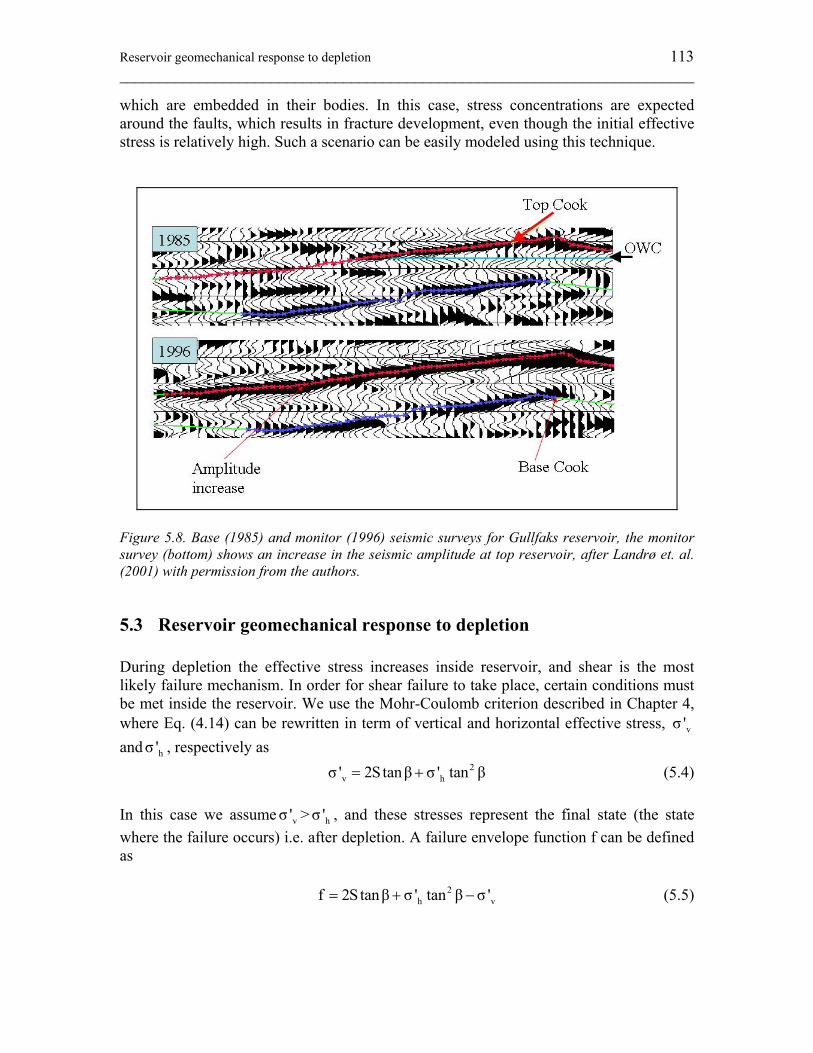
Reservoir geomechanical response to depletion 113 ________________________________________________________________________
which are embedded in their bodies. In this case, stress concentrations are expected around the faults, which results in fracture development, even though the initial effective stress is relatively high. Such a scenario can be easily modeled using this technique.
Figure 5.8. Base (1985) and monitor (1996) seismic surveys for Gullfaks reservoir, the monitor survey (bottom) shows an increase in the seismic amplitude at top reservoir, after Landrø et. al. (2001) with permission from the authors.
5.3 Reservoir geomechanical response to depletion During depletion the effective stress increases inside reservoir, and shear is the most likely failure mechanism. In order for shear failure to take place, certain conditions must be met inside the reservoir. We use the Mohr-Coulomb criterion described in Chapter 4, where Eq. (4.14) can be rewritten in term of vertical and horizontal effective stress, vσ ' and hσ ' , respectively as 2
v hσ ' 2S tanβ σ ' tan β= + (5.4) In this case we assume vσ ' > hσ ' , and these stresses represent the final state (the state where the failure occurs) i.e. after depletion. A failure envelope function f can be defined as 2
h vf 2S tanβ σ ' tan β σ '= + − (5.5)
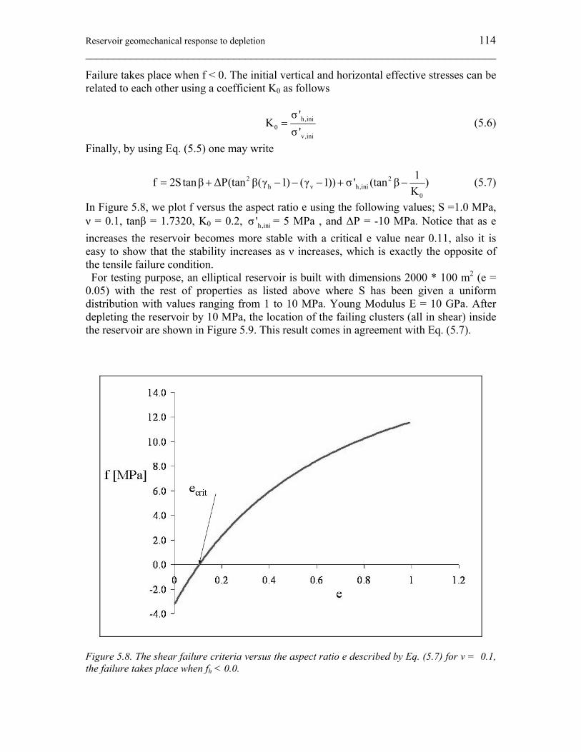
Reservoir geomechanical response to depletion 114 ________________________________________________________________________
Failure takes place when f < 0. The initial vertical and horizontal effective stresses can be related to each other using a coefficient K0 as follows
h,ini0
v,ini
σ 'K
σ '= (5.6)
Finally, by using Eq. (5.5) one may write
2 2h v h,ini
0
1f 2Stanβ ΔP(tan β(γ 1) (γ 1)) σ ' (tan β )K
= + − − − + − (5.7)
In Figure 5.8, we plot f versus the aspect ratio e using the following values; S =1.0 MPa, ν = 0.1, tanβ = 1.7320, K0 = 0.2, h,iniσ ' = 5 MPa , and ΔP = -10 MPa. Notice that as e increases the reservoir becomes more stable with a critical e value near 0.11, also it is easy to show that the stability increases as ν increases, which is exactly the opposite of the tensile failure condition. For testing purpose, an elliptical reservoir is built with dimensions 2000 * 100 m2 (e = 0.05) with the rest of properties as listed above where S has been given a uniform distribution with values ranging from 1 to 10 MPa. Young Modulus E = 10 GPa. After depleting the reservoir by 10 MPa, the location of the failing clusters (all in shear) inside the reservoir are shown in Figure 5.9. This result comes in agreement with Eq. (5.7).
Figure 5.8. The shear failure criteria versus the aspect ratio e described by Eq. (5.7) for ν = 0.1, the failure takes place when fh < 0.0.
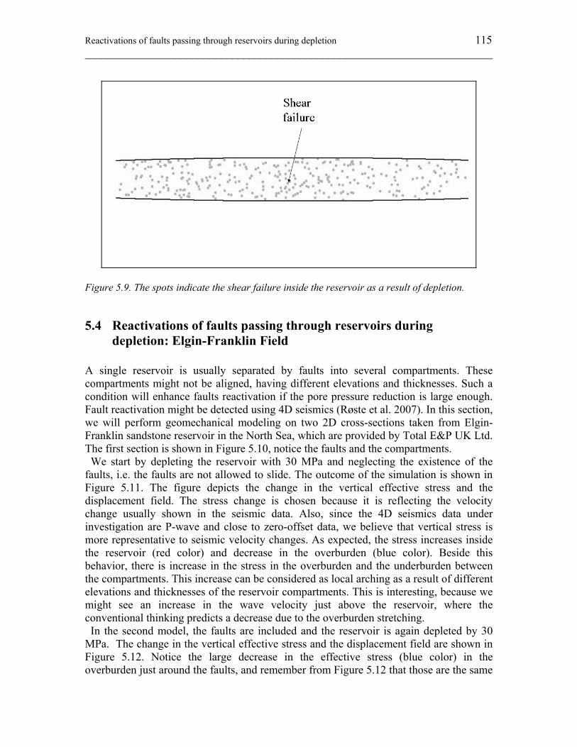
Reactivations of faults passing through reservoirs during depletion 115 ________________________________________________________________________
Figure 5.9. The spots indicate the shear failure inside the reservoir as a result of depletion.
5.4 Reactivations of faults passing through reservoirs during depletion: Elgin-Franklin Field
A single reservoir is usually separated by faults into several compartments. These compartments might not be aligned, having different elevations and thicknesses. Such a condition will enhance faults reactivation if the pore pressure reduction is large enough. Fault reactivation might be detected using 4D seismics (Røste et al. 2007). In this section, we will perform geomechanical modeling on two 2D cross-sections taken from Elgin-Franklin sandstone reservoir in the North Sea, which are provided by Total E&P UK Ltd. The first section is shown in Figure 5.10, notice the faults and the compartments. We start by depleting the reservoir with 30 MPa and neglecting the existence of the faults, i.e. the faults are not allowed to slide. The outcome of the simulation is shown in Figure 5.11. The figure depicts the change in the vertical effective stress and the displacement field. The stress change is chosen because it is reflecting the velocity change usually shown in the seismic data. Also, since the 4D seismics data under investigation are P-wave and close to zero-offset data, we believe that vertical stress is more representative to seismic velocity changes. As expected, the stress increases inside the reservoir (red color) and decrease in the overburden (blue color). Beside this behavior, there is increase in the stress in the overburden and the underburden between the compartments. This increase can be considered as local arching as a result of different elevations and thicknesses of the reservoir compartments. This is interesting, because we might see an increase in the wave velocity just above the reservoir, where the conventional thinking predicts a decrease due to the overburden stretching. In the second model, the faults are included and the reservoir is again depleted by 30 MPa. The change in the vertical effective stress and the displacement field are shown in Figure 5.12. Notice the large decrease in the effective stress (blue color) in the overburden just around the faults, and remember from Figure 5.12 that those are the same
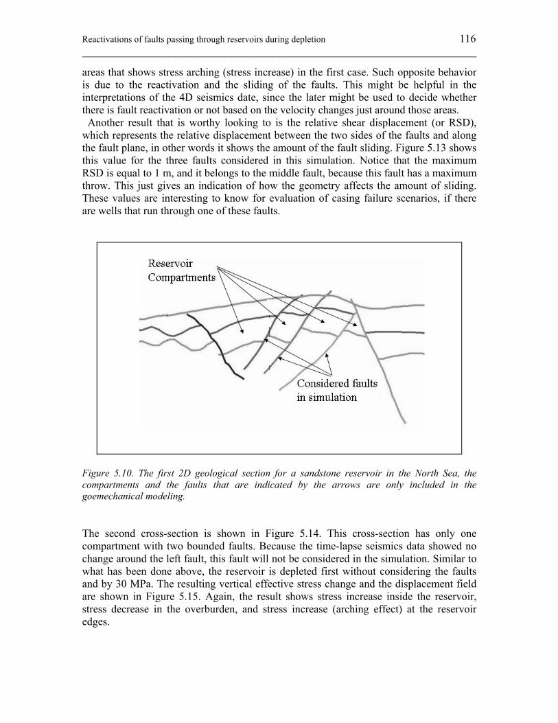
Reactivations of faults passing through reservoirs during depletion 116 ________________________________________________________________________
areas that shows stress arching (stress increase) in the first case. Such opposite behavior is due to the reactivation and the sliding of the faults. This might be helpful in the interpretations of the 4D seismics date, since the later might be used to decide whether there is fault reactivation or not based on the velocity changes just around those areas. Another result that is worthy looking to is the relative shear displacement (or RSD), which represents the relative displacement between the two sides of the faults and along the fault plane, in other words it shows the amount of the fault sliding. Figure 5.13 shows this value for the three faults considered in this simulation. Notice that the maximum RSD is equal to 1 m, and it belongs to the middle fault, because this fault has a maximum throw. This just gives an indication of how the geometry affects the amount of sliding. These values are interesting to know for evaluation of casing failure scenarios, if there are wells that run through one of these faults.
Figure 5.10. The first 2D geological section for a sandstone reservoir in the North Sea, the compartments and the faults that are indicated by the arrows are only included in the goemechanical modeling. The second cross-section is shown in Figure 5.14. This cross-section has only one compartment with two bounded faults. Because the time-lapse seismics data showed no change around the left fault, this fault will not be considered in the simulation. Similar to what has been done above, the reservoir is depleted first without considering the faults and by 30 MPa. The resulting vertical effective stress change and the displacement field are shown in Figure 5.15. Again, the result shows stress increase inside the reservoir, stress decrease in the overburden, and stress increase (arching effect) at the reservoir edges.
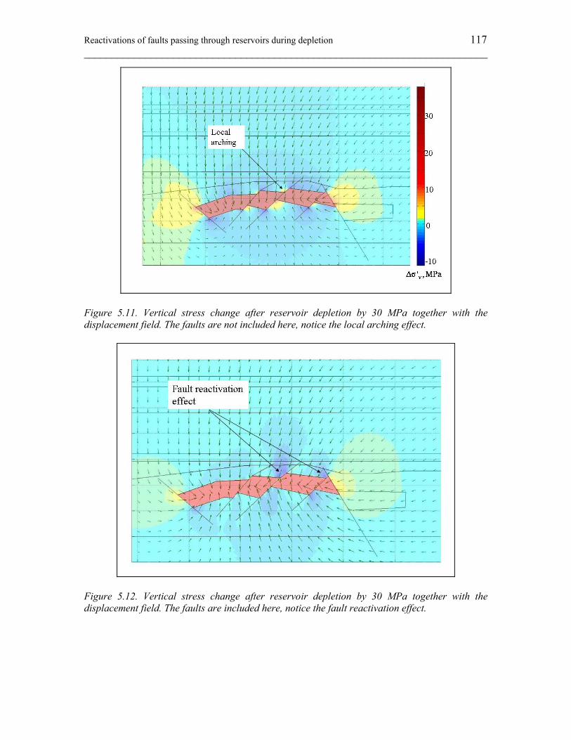
Reactivations of faults passing through reservoirs during depletion 117 ________________________________________________________________________
Figure 5.11. Vertical stress change after reservoir depletion by 30 MPa together with the displacement field. The faults are not included here, notice the local arching effect.
Figure 5.12. Vertical stress change after reservoir depletion by 30 MPa together with the displacement field. The faults are included here, notice the fault reactivation effect.
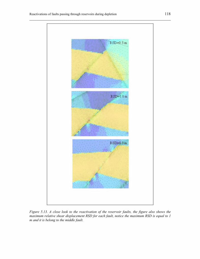
Reactivations of faults passing through reservoirs during depletion 118 ________________________________________________________________________
Figure 5.13. A close look to the reactivation of the reservoir faults, the figure also shows the maximum relative shear displacement RSD for each fault, notice the maximum RSD is equal to 1 m and it is belong to the middle fault.
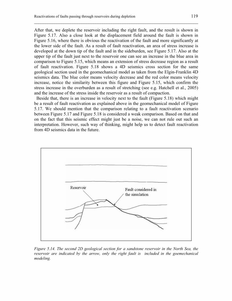
Reactivations of faults passing through reservoirs during depletion 119 ________________________________________________________________________
After that, we deplete the reservoir including the right fault, and the result is shown in Figure 5.17. Also a close look at the displacement field around the fault is shown in Figure 5.16, where there is obvious the reactivation of the fault and more significantly at the lower side of the fault. As a result of fault reactivation, an area of stress increase is developed at the down tip of the fault and in the sideburden, see Figure 5.17. Also at the upper tip of the fault just next to the reservoir one can see an increase in the blue area in comparison to Figure 5.15, which means an extension of stress decrease region as a result of fault reactivation. Figure 5.18 shows a 4D seismics cross section for the same geological section used in the geomechanical model as taken from the Elgin-Franklin 4D seismics data. The blue color means velocity decrease and the red color means velocity increase, notice the similarity between this figure and Figure 5.15, which confirm the stress increase in the overburden as a result of stretching (see e.g. Hatchell et al., 2005) and the increase of the stress inside the reservoir as a result of compaction. Beside that, there is an increase in velocity next to the fault (Figure 5.18) which might be a result of fault reactivation as explained above in the geomechanical model of Figure 5.17. We should mention that the comparison relating to a fault reactivation scenario between Figure 5.17 and Figure 5.18 is considered a weak comparison. Based on that and on the fact that this seismic effect might just be a noise, we can not rule out such an interpretation. However, such way of thinking, might help us to detect fault reactivation from 4D seismics data in the future.
Figure 5.14. The second 2D geological section for a sandstone reservoir in the North Sea, the reservoir are indicated by the arrow, only the right fault is included in the goemechanical modeling.
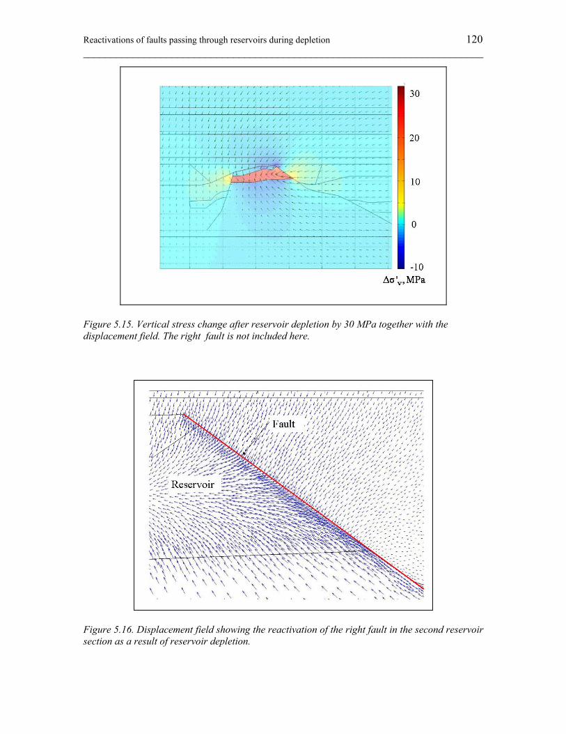
Reactivations of faults passing through reservoirs during depletion 120 ________________________________________________________________________
Figure 5.15. Vertical stress change after reservoir depletion by 30 MPa together with the displacement field. The right fault is not included here.
Figure 5.16. Displacement field showing the reactivation of the right fault in the second reservoir section as a result of reservoir depletion.
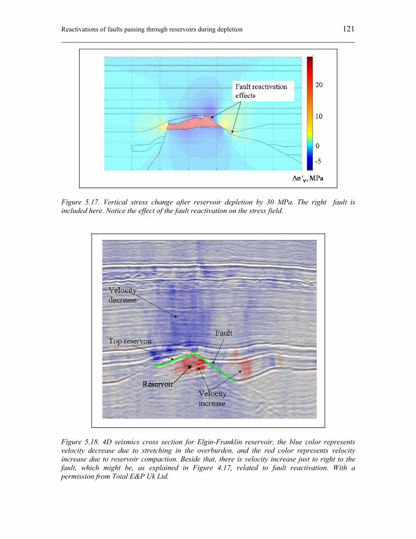
Reactivations of faults passing through reservoirs during depletion 121 ________________________________________________________________________
Figure 5.17. Vertical stress change after reservoir depletion by 30 MPa. The right fault is included here. Notice the effect of the fault reactivation on the stress field.
Figure 5.18. 4D seismics cross section for Elgin-Franklin reservoir, the blue color represents velocity decrease due to stretching in the overburden, and the red color represents velocity increase due to reservoir compaction. Beside that, there is velocity increase just to right to the fault, which might be, as explained in Figure 4.17, related to fault reactivation. With a permission from Total E&P Uk Ltd.
Building velocity model of Gullfaks synthetic model 122 ________________________________________________________________________
5.5 Building velocity model of Gullfaks model for time-lapse seismics study
After obtaining the amount and the distribution of fractures from the geomechanical model, it is now possible to use these fractures to update the velocity model for a time-lapse seismics study. One way of doing so is to divide the model into several control volumes, and then use Rock Physics models based on crack density and crack orientation to update the velocity model. However, this requires a very fine model so that there is a sufficient amount of control volumes. This is essential to avoid dependency on the size and the number of the control volumes chosen. As an alternative, we decided to choose each failing cluster as a control volume, remember each failing cluster has the possibility of having 0, 1, 2, or 3 cracks. Then an effective medium theory for a cracked medium explained in Chapter 1 (Budiansky et al., 1976) is used to update the velocity for each cluster. This model assumes isotropy. This approach results in copying the fractures as they are from the geomechanical model to the velocity models where the velocity change depends on (among other things) the number of cracks per cluster (0, 1, 2, or 3). Of course, such an approach requires calibration from some experimental or field data to assure that the contribution of these fractures resemble those in the real rocks. For Gullfaks 2D synthetic model, we use some published data to update the velocity model (Kvam et. al., 2005), where the values of P-wave and S-wave velocities in the reservoir are Vp = 2630 m/s, Vs = 1340 m/s, and the reservoir density is ρ = 2350 kg/m3. The velocity change model can now be easily constructed. Figure 5.19 shows the reduction in P-wave (up) and S-wave (down) velocities for the low horizontal effective stress scenario, the mean value of ΔVp = 400 m/s and of ΔVs = 100 m/s. Figure 5.20 shows the same thing but for low vertical effective stress scenario, where the mean value of ΔVp = 670 m/s and of ΔVs = 200 m/s. Of course, since the model needs calibration, the real values might differ from those shown in the figures.
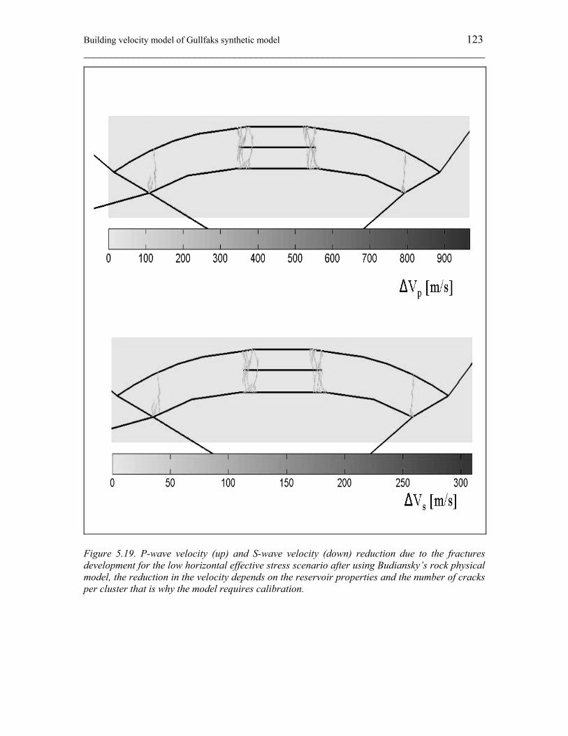
Building velocity model of Gullfaks synthetic model 123 ________________________________________________________________________
Figure 5.19. P-wave velocity (up) and S-wave velocity (down) reduction due to the fractures development for the low horizontal effective stress scenario after using Budiansky’s rock physical model, the reduction in the velocity depends on the reservoir properties and the number of cracks per cluster that is why the model requires calibration.
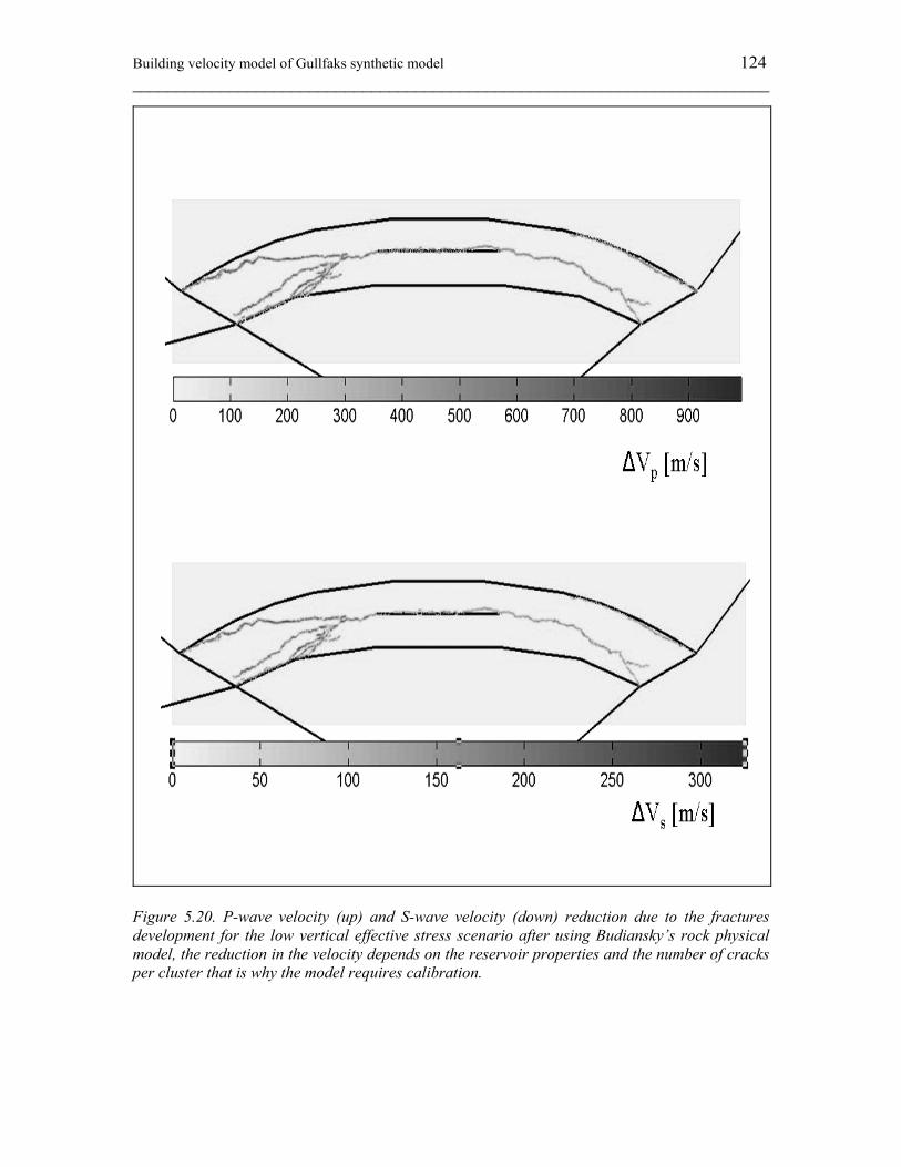
Building velocity model of Gullfaks synthetic model 124 ________________________________________________________________________
Figure 5.20. P-wave velocity (up) and S-wave velocity (down) reduction due to the fractures development for the low vertical effective stress scenario after using Budiansky’s rock physical model, the reduction in the velocity depends on the reservoir properties and the number of cracks per cluster that is why the model requires calibration.
Chapter 6: Conclusion 125 ________________________________________________________________________
6 Conclusion In Chapter 2 we showed the possibilities of using Discrete Element Method (DEM) in modeling reservoir geomechanics. For the elastic limit, the comparison of the displacement field between DEM and the analytical solution, derived in Chapter 1, was fairly good. The misfit was mainly related to the model boundary, which requires a larger model to be built, and since DEM is an expensive method in term of elements number, using continuum coarse grid, coupled with the DEM region, for the model far field is a possible solution. The main problem in fitting the stresses was related to the way the stress was measured, which was based on using the element area. In PFC, the best way to avoid such a problem is to use measurement circles to measure the stress, however this requires that each measurement circle contains a sufficient amount of elements, which was not practical for our coarse model. As it was shown in Chapter 3 that by taken the above points into consideration, a very good fit was achieved. The fracture development and fault reactivation, when modeling beyond the elasticity limit, came in agreement of what theory predicts, (see e.g. Segall et al., 1998). For example, by comparing Figure 2.9 to Figure 1.11, one can notice how the fracture propagation follows the contour of zero horizontal stress line. Relations to relate DEM parameters to rock properties were derived in Chapter 3. Such relations will facilitate feeding geomechanical models with correct properties. The relations were derived for two categories: dense packing, and loose random packing. For the dense packing, the dynamic and the static relations are the same, and a limitation on the maximum Vp/Vs is found (Vp/Vs < 3 ) which corresponds to a maximum Poisson’s ratio ν < 0.25 (plane strain). The static behavior for the loose random packing deviates from the dynamic behavior. The dynamic behavior can still be given by some analytical relation with the same limitation like that for the dense packing, while empirical relations for the static behavior have to be obtained based on numerical tests. It is also important to mention that the static Poisson’s ratio for loose random packing is not limited by 0.25. It was shown that if the particle rotation is prevented, a new expression for the shear wave has to be derived after using the Cosserat continuum theory, the new expression for the shear wave allows the shear wave to travel faster than the pressure wave, which is unrealistic for isotropic rocks. Based on the study performed in this thesis, we conclude that there are three main limitations hinder the use of (particle-based) DEM in modeling large-scale reservoir geomechanics. First, the maximum P-wave/S-wave ratio is limited by (Vp/Vs < 3 ). Second, it is difficult to derive relations for failure properties just like it was done for elastic properties, and numerical tests have to be done each time a geomechanical model is built. Third, there are always difficulties in building geomechanical models and installing complicated initial stress conditions, usually given for hydrocarbon reservoirs, using DEM. Because of the limitations described above, a modified discrete element approach was proposed. The modified approach works on clusters made of three elements each. For each cluster the micro stiffness matrix (K) are derived based on rock properties given by the macro stiffness matrix (C). K contains the regular normal stiffness parameters for all
Chapter 6: Conclusion 126 ________________________________________________________________________
contacts in the cluster knm, and the newly introduced stiffness parameters aij. The shear stiffness parameter is calculated using the ratio r (ksm = r * knm). That means in order to model any material using this method, one needs C and r as input parameters, beside that the shear and the tensile strengths are also required. Before failure the cluster behaves like continuum models (e.g. FEM, & FDM) and after failure the cluster behaves similar to regular DEM. The method was tested successfully by comparing it to FEM, and by performing crack propagation and uniaxial compression tests. For intact cluster, all the shear forces are set to zero, and the shear forces start to build up only when the cluster fails. However, in more generalized approach, the shear forces can be included before the cluster fails. In this case, the micro stiffness matrix (K) should be calculated using the procedure described in Chapter 4.6 instead, and the particle rotation has to be accounted for. Fluid coupling scheme (based on Finite Difference) to be used with the modified approach was proposed. In such a scheme, the domain is discretized into a network of pipes that match the contacts in the clusters. This will allow fluid flow through fractures (pipes) as they are developed. The scheme was tested successfully by comparing it to analytical solution. Analytical expressions for the stress path coefficients were used to study the condition of rock failure inside reservoirs during both fluid injection and depletion. It was shown that if the injected fluid pressure rises above the effective stresses, tensile failure may happen, depending on reservoirs properties and geometry. Then, the modified approach was used to model reservoir geomechanical behavior and the result of this modeling was compared to these analytical solutions. The method, then, was used to model a reservoir geomechanical response during fluid injection for a case study of Gullfaks field. The models showed possibilities of fractures development, these fractures may form vertically or horizontally depends on the initial effective stress. The fractures were also concentrated on the well’s and the reservoir’s edges. It was also shown that the fluid coupling and reservoir geometry play an important rule in controlling when and how the fractures develop, in a way that can not be predicted by the analytical solution alone. The result was compared to 4D seismics cross sections taken from Gullfaks field, and it was shown, according to the seismic data, that the horizontal fractures scenario is more likely the case. This comes in agreement with the goemechanical model, since the vertical stress path coefficient is much less than the horizontal one, which makes it more difficult for the vertical fracture to develop than for the horizontal one, see Figure 5.1 for more details. The modified discrete element approach was used to model the effect of fault reactivation on changing the stress field around reservoirs during depletion. Two cross sections taken from Elgin-Franklin field were used to study such a case. The result shows that if a fault is reactivated, the stress change around the reservoir is different from the case of no fault reactivation. The result for the geomechanical model of one of Elgin-Franklin cross-sections was compared to 4D seismics data for the same section, where it was noticed an increase of the wave velocity near the fault, which mimics the effect shown by the goemechanical model. To what extent, this seismic anomaly may correspond to fault reactivation remains unknown, since this anomaly might be just a noise, however such an interpretation may help us in the future when more 4D seismics data are coming.
References 127 ________________________________________________________________________
References Addis, M. A. 1997. The stress-depletion response of reservoirs. SPE 38720, 11 pp. Bachrach, R. & Davorkin, J. & Nur, A. M. 2000. Seismic velocities and Poisson’s ratio of
shallow unconsolidated sands. Geophysics, Vol. 65: 559-564. Biot, M. A. 1941. General theory of three-dimensional consolidation. J. Appl. Phys., 12:155-164. Biot, M. A. 1962. Mechanics of deformation and acoustic propagation in porous media. J. Appl.
Phys., 33:1482-1498. Brignoli, M., Pellegrino, A., Santarelli, F.J., Musso, G. and Barla, G. 1997. Continuous and
discontinuous deformations above compacting reservoirs; consequences upon the lateral extension of the subsidence bowl, Int. J. Rock Mech. and Min. Sci. 34 (3–4).
Budiansky, B. & O’Connell, R. J. 1976. Elastic moduli of a cracked solid. International journal of solid and structure, 12: 81-97.
Chen, W. F. & Mizuno, E. 1990. Nonlinear analysis in soil mechanics: theory and implementation. Elsevier B. V., Amsterdam.
Cundall, P.A. & Strack, O.D.L. 1979. A discrete numerical model for granular assemblies. Geotechnique 29(1): 47–65.
Cundall, P. A. 1987. “Distinct element models of Rock and soil structure”, in analytical and computational methods in engineering rock mechanics, Ch. 4: 129-163, E. T. Brown, Ed. London: Allen & Unwin.
Davies, J. H. 2003. Elastic field in a semi-infinite solid due to thermal expansion or a coherently misfitting inclusion. ASME Journal of Applied Mechanics. 70: 655-660.
De Hoop, A. T. 1960. The Surface Line Source Problem. Appl. Sci. Res. Vol. B8: 349-356. Digby, P. J. 1981. The effective elastic moduli of porous granular rocks. J. Appl. Mech., 48:803-
808. Du, J. & Olson, J. E. 2001. A poroelastic reservoir model for predicting subsidence and mapping
surface pressure fronts. Journal of Petroleum Science and Engineering. Vol. 30: 181-197. Duffaut, K. & Landrø, M. 2007. Vp/Vs ratio versus differential stress and rock consolidation – a
comparison between rock models and time-lapse AVO data. Geophysics, Vol. 72, N.5:C81-C94.
Elhers, W. & Ramm, E. & Diebels, S. & D’Addetta, G. A. 2003. From particle ensembles to Cosserat continua: homogenization of contact forces towards stresses and couple stresses. Int. J. Solids Structures, 40: 6681-6702.
Eringen, A. C. 1968. Theory of micropolar elasticity. In Fracture: an advanced treatise (Ed. Liebowitz, H.), Academic Press, Inc.
Eshelby, J. D. 1957. The determination of the elastic field of an ellipsoidal inclusion, and related problems. Proc. Roy. Soc. London ser., A241: 376-396.
Ferrari, M. & Granik, V. T. & Imam, A. & Nadeau, J. C. 1997. Advances in doublet mechanics. Springer.
Fjær, E. & Holt, R. M. & Horsrud, P. & Raaen, A. M. & Risnes, R. 2008. Petroleum related rock mechanics. Elsevier Science Publishers B.V.
Fjær, E. 2006. Modeling the stress dependence of elastic wave velocities in soft rocks. ARMA/USRMS 06-1070.
Gambolati, G. & Teatini, P. & Tomasi, L. 1999. Stress-strain analysis in productive gas/oil reservoirs. Int. J. Numer. Anal. Meth. Geomech. 23: 1495–1519.
Gambolati, G., Ferronato, M. & Teatini, P. & Deidda, R., & Lecca, G. 2001. Finite element analysis of land subsidence above depleted reservoirs with pore pressure gradient and total stress formulations, Int. J. Numer. Anal. Meth. Geomech. 25: 307-327.
Geertsma, J. 1957. A remark on the analogy between thermoelasticity and the elasticity of saturated porous media. Journal of Mechanics and Physics of Solids, Vol. 6: 13-16.
Geertsma, J. 1973. A basic theory of subsidence due to reservoir compaction: the homogeneous case. Trans. Royal Dutch Soc. Geol. & Mining Eng. 28: 43-62.
Gommesen, L. and Fabricius, I.L. 2001. Dynamic and static elastic moduli of North Sea chalk. Physics and Chemistry of the Earth, Part A, Solid Earth and Geodesy: 63-68.
Goodman, R. E. 1980. Introduction to Rock Mechanics. New York: John Wiley & Sons.
References 128 ________________________________________________________________________
Grasso, J. R. 1992. Mechanics of seismic instabilities induced by the recovery of hydrocarbons. Pure & Applied Geophysics, Vol. 139: 507.
Gutlerrez, M. & Hansteen, H. 1994. Fully coupled analysis of reservoir compaction and subsidence. SPE 28900.
Gutierrez, M. & Lewis, R.W. 1998. The role of geomechanics in reservoir simulation. SPE/ISRM 47392, In Proc. EUROCK’98, vol. II: 439-448.
Hall, S. A. 2006. A methodology for 7D warping and deformation monitoring using time-lapse seismic data. Geophysics, Vol. 71: O21-O31.
Hashin, Z. & Shtrikman, S. 1963. A variational approach to elastic behavior of multiphase materials. J. Mech. Solids. 11:127-140.
Hatchell, P. & Bourne, S. 2005. Rocks under strain: strain-induced time-lapse time shifts are observed for depleting reservoirs. The Leading Edge 24: 1222-1225.
Hazzard, J.F. & Young, R.P. 2000. Simulating acoustic emissions in bonded-particle models of rock. Int. J. Rock Mech. and Min. Sci. 37: 867-872.
Hertz, H. 1882. Über die Berühhrung fester elastischer Körper. J reine und angewandte Mathematik, 92:156-171.
Hettema, M.H.H. & Schutjens, P.M.T.M. & Verboom, B.J.M. & Gussinklo, H.J.1998. Productioninduced compaction of sandstone reservoirs: The strong influence of field stress. SPE50630, 8 pp.
Holt, R.M. & Flornes, O. & Li, L. & Fjær, E. 2004. Consequences of depletion-induced stress changes on reservoir compaction and recovery. In Proc.Gulf-Rock (eds.Arma/Narms) 04-589, ARMA/NARMS, 10 pp.
Holt, R.M. & Kjølaas, J. & Larsen, I. & Li, L. & Pillitteri, A.G. & Sønstebø, E.F. 2005. Comparison between controlled laboratory experiments and discrete particle simulations of rock mechanical behaviour, Int. J. Rock Mech. and Min. Sci. 42: 985-995.
Hori, M. & Oguni, K. & Sakaguchi, H. 2005. Proposal of FEM implemented with particle discretization for analysis of failure phenomena. J. Mech. Phys. Solid., 53: 681-703.
Horsrud, P. 2001. Estimating mechanical properties of shale from empirical correlations. SPE Drill. Complet., pp. 68-73
Hudson, J. A. 1981. Wave speed and attenuation of elastic waves in material containing cracks. Geophys. J. R. Astr. Soc., 64: 133-150.
Itasca Consulting Group Inc. 2004. PFC2D user’s manuals. Ivar, M. D. & Potyondy, D. O. & Pierce, M. & Cundall, P. A. 2008. The Smooth-Joint Contact
Model. 2-page extended abstract for 8th World Congress on Computational Mechanics (WCCM8), Venice, Italy.
Jing, L. & Hudson, J.A. 2002. Numerical methods in rock mechanics. Int. J. Rock Mech. and Min. Sci., 39:409-427.
Johnson, K. L. 1985. Contact mechanics. Cambridge University Press. Johnston, D. H. & McKenny, R. S. & Verbeek, J. & Almond, J.1998. Time-lapse seismic analysis
of Fulmar Field. The Leading Edge, 17: 1420-1428. Kenter, C.J. & Blanton, T.L. & Schreppers, G.M.A. & Baaijens, M.N. & Ramos, G.G. 1998.
Compaction study for Shearwater Field, SPE/ISRM 47280. In Proc. EUROCK’98, Vol. II: 63-68.
Kenter, C.J. & Beukel, A.V. D. & Hatshell, P. & Marno, K. & Molenaar, M. 2004. Evaluation of reservoir characteristics from timeshifts in the overburden, In Proc. Gulf-Rock (eds. Arma/Narms) 04-627, ARMA/NARMS.
Kosloff, D. & Scott, R.F. & Scranton, J.1980. Finite element simulation of Wilmington oil field subsidence: 1. Linear modeling. Tectonophysics 65: 339-368.
Koutsabeloulis, N. C. & Hope, S. A.1998. ‘‘Coupled’’ stress / fluid / thermal multi-phase reservoir simulation studies incorporating rock mechanics. SPE/ISRM 47393. In Proc. EUROCK’98 Vol. II: 449-454.
Kvam, Ø. & Landrø, M. 2005. Pore-pressure detection sensitivities tested with time-lapse seismic data. Geophysics, Vol. 70, N. 6: O39-O50.
Kwon, Young W. & Bang, Hyochoong. 1997. The finite element method using matlab. CRC Press Inc., New York.
Landrø, M. 2001. Discrimination between pressure and fluid saturation changes from time-lapse seismic data. Geophysics, Vol. 66: 836-844.
References 129 ________________________________________________________________________
Landrø, M. & Digranes, P. & Strønen, L. K. 2001. Mapping reservoir pressure and saturation changes using seismic methods-possibilities andlimitations. First Break, V. 19. 12.
Landrø. M. & Stammeijer, J. 2004. Quantitative estimation of compaction and velocity changes using 4D impedence and traveltime changes. Geophysics, Vol. 69: 949-957.
Lewis, R.W. & Makurat, A. & Pao, K.S. 2003. Fully coupled modeling of subsidence and reservoir compaction of North Sea oil fields. Hydrogeology J. 11:142-161.
Li, L. 2002. Particle scale reservoir mechanics. PHD Thesis, NTNU, Trondheim, Norway. Li, L. & Holt, R.M. 2002. Particle scale reservoir mechanics, Oil and Gas Science and
Technology-Revue de l’Institut Français du Pétrole 57: 525-538. Li, L. & Holt, R.M. 2004. A study on the calculation of particle volumetric deformation in a fluid
coupled PFC model. In Numerical Modeling in Micromechanics via Particle Methods (eds. Shimizu, Hart and Cundall), (A. A. Balkema 2004), pp. 273-279.
Liebowitz, H. 1968. Fracture: an advanced treatise. Academic Press, Inc. Longuemare, P. & Mainguy, M. & Lemonnier, P. & Onaisi, A. & Gérard, C. 2002).
Geomechanics inreservoir simulation: Overview of coupling methods and field case study. Oil and Gas Science andTechnology -Revue de l’Institut Français du Pétrole 57 : 471-483.
Lumley, D. E. & Behrens, R. A. & Wang, Z.1997. Assessing the technicalrisk of a 4-D seismic project. The Leading Edge, 16: 1287-1291.
Lumley, D. E. 2001.Time-lapse seismic reservoir monitoring. Geophysics, Vol. 66: 50-53. Mahi, A. 2003. Stress path of depleting reservoirs. MSc Thesis, NTNU (Norwegian University of
Science and Technology). Maxwell, S.C. & Urbancic, T. 2001. The role of passive microseismic monitoring in the
instrumented oil field, The Leading Edge, 636-639. Mindlin, R. D. 1949. Compliance of elastic body in contact. J. App. Mech., 16: 259-268. Mindlin R. D. & Cheng, D. H. 1950. Nuclei of strain in the semi-infinite solid. J. App. Phys.,
Vol. 21: 926. Mindlin, R. D. 1965. Stress function for a Cosserate continuum. Int. J. Solids Structures, Vol. 1 :
265-271. Morita, N. & Whitfill, D.L. & Nygaard, O. & Bale, A. 1989. A quick method to determine
subsidence,reservoir compaction, and in-situ stress induced by reservoir depletion. JPT Jan.89: 71-79.
Mulders, F. M. M. 2003. Modelling of stress development and fault slip in and around a producing gas reservoir. Ph.D. Thesis, TU Delft, Netherlands.
Munjiza, Ante. 2004. The combined finite-discrete element method. John Wiley & sons Ltd, England.
Oded, K. & Ze’ev, R. & Gidon, B. 2003. Faults and their associated host rock deformation: Part I.Structure of small faults in a quartz–syenite body, southern Israel, J. Struct. Geol. 25:1675-1689.
Osorio, J.G. & Chen, H.Y. & Teufel, L.W. & Schaffer, S.1998. A two-domain, 3-D, fully coupled fluidflow/geomechanical simulation model for reservoirs with stress-sensitive mechanical and fluid-flowproperties. SPE/ISRM 47397. In Proc. EUROCK’98, Vol. II: 455–464.
Pande, G. N. & Beer, G. & Williams, J. R. 1990. Numerical Methods in Rock Mechanics. Wiley. Papamichos, E. & Vardoulakis, I. & Heil, L. K. 2001. Overburden modeling above a compacting
reservoir using a trap door apparatus. Phys. Chem. Earth (A) 26: 69-74. Potyondy, D.O. & Cundall, P. A. 2004. A bonded particle model for rock. Int. J. Rock Mech. And
Min. Sci., 41:1329-1364. Rudnicki, J.W. 1999. Alteration of regional stress by reservoirs and other inhomogeneities:
Stabilizing or destabilizing?. Proc. Int. Congress on Rock Mechanics, eds. G. Vouille and P. Berest, ISRM, Vol. 3: 1629-1637.
Røste, Thomas & Landrø, Martin & Hatchell, Paul. 2007. Monitoring overburden layer changes and fault movements from time-lapse seismic data on the Valhall Field. Geophys. J. Int., Vol 170:1100-1118.
Sayers, C. M. & Kachanov, M. 1995. Microcrack-induced elastic wave anisotropy of brittle rocks. Journal of Geophysical Research, Vol 100 (No. B3): 4149-4156.
Segall, P. & Fitzgerald, S.D. 1998. A note on induced stress changes in hydrocarbon and geothermal reservoirs. Tectonophysics 289: 117-28.
Settari, A. & Mourits, F. M. 1994. Coupling of geomechanics and reservoir simulation models, Computer Methods and Advances in Geomechanics, 2151-2158.
References 130 ________________________________________________________________________
Shi GH. 1991. Manifold method of material analysis. In Transactions of the 9th Army Conference On Applied Mathematics and Computing, Report No. 92-1, U.S. Army Research Office.
Shimizu, Y. 2004 . Fluid coupling in PFC2-D and PFC3-D. In Numerical Modeling in Micromechanics via Particle Methods, (eds. Shimizu, Hart and Cundall) (A. A. Balkema 2004), pp. 281-287.
Sønneland, L. & Veire, H. H. & Raymond, B. & Signer, C. & Pedersen, L. & Ryan, S. & Sayers, C. 1997. Seismic reservoir monitoring on Gullfaks. The Leading Edge, 16: 1247-1252.
Teufel, L. W. & Rhett, D. W. & Farrell, H. E. 1991. Effect of reservoir depletion and pore pressure drawdown on in situ stress and deformation in the Ekofisk field. In Rock Mechanics as a Multidisciplinary Science (ed. J.C. Roegiers) (A.A. Balkema 1991), pp. 63-72.
Timoshenko, S. & Goodier, J. N. 1970. Theory of elasticity. McGraw-Hill. Wilkins, M. L. 1964. “Calculation of elastic-plastic flow”, in Methods in computational physics,
Fundamental methods in hydrodynamics, Vol. 3: 211-263. Academic Press, New York. Walton, K. 1987. The effective elastic moduli of a random packing of spheres. J. Mech. Phys.
Solid. 35(2): 213-226. Zienkiewicz, O. C. 1991. The Finite Element Method in Engineering Geoscience (4th edition).
McGraw-Hill. Zienkiewicz, O. C. & Taylor, R. L. 2000. The finite element method, The basic, Vol. 1.
Butterworth-Heinemann, Oxford.
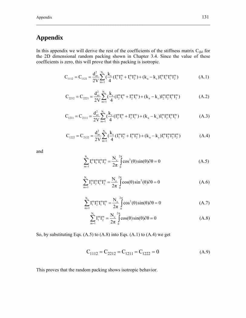
Appendix 131 ________________________________________________________________________
Appendix In this appendix we will derive the rest of the coefficients of the stiffness matrix Cijkl for the 2D dimensional random packing shown in Chapter 3.4. Since the value of these coefficients is zero, this will prove that this packing is isotropic.
cN2
m m m m m m m mav s1112 1121 1 2 1 2 n s 1 1 1 2
m 1
d kC C ( (I I I I ) (k k )I I I I )2V 4=
= = + + −∑ (A.1)
cN2
m m m m m m m mav s2212 2221 2 1 2 1 n s 2 2 1 2
m 1
d kC C ( (I I I I ) (k k )I I I I )2V 4=
= = + + −∑ (A.2)
cN2
m m m m m m m mav s1211 2111 2 1 2 1 n s 1 2 1 1
m 1
d kC C ( (I I I I ) (k k )I I I I )2V 4=
= = + + −∑ (A.3)
cN2
m m m m m m m mav s1222 2122 1 2 1 2 n s 1 2 2 2
m 1
d kC C ( (I I I I ) (k k )I I I I )2V 4=
= = + + −∑ (A.4)
and
c 2πN
m m m m 3c1 1 1 2
m 1 0
NI I I I cos (θ)sin(θ) θ 02π=
= ∂ =∑ ∫ (A.5)
c 2πN
m m m m 3c2 2 1 2
m 1 0
NI I I I cos(θ)sin (θ) θ 02π=
= ∂ =∑ ∫ (A.6)
c 2πN
m m m m 3c1 2 1 1
m 1 0
NI I I I cos (θ)sin(θ) θ 02π=
= ∂ =∑ ∫ (A.7)
c 2πN
m m c1 2
m 1 0
NI I cos(θ)sin(θ) θ 02π=
= ∂ =∑ ∫ (A.8)
So, by substituting Eqs. (A.5) to (A.8) into Eqs. (A.1) to (A.4) we get 1112 2212 1211 1222C C C C 0= = = = (A.9) This proves that the random packing shows isotropic behavior.