Doctoral Dissertation London Business School University of ...

1

Doctoral Dissertation

London Business School University of London

Essays on the decisions of investors and fund managers

Sam Wylie

March 1999

2

Acknowledgements

This thesis is dedicated to Tracey for her support and patience and to our sons

Reuben and Angus who came along in time to help finish.

For financial support I thank Mercury Asset Management, Salomon Brothers and

The Overseas Students Research Award Scheme. For data I thank John Morrell Pty

Ltd and the WM Company. For advice on institutional arrangements I am indebted

to many people but especially Nigel Foster, Graham Dixon, Mark Bradshaw, Gordon

Bagot and Linda-Jane Coffin.

For advice and helpful discussions I thank Walter Torous, Mark Britten-Jones,

Michael Brennan, Henri Servaes, David Pyle, James Dow, Dick Brealey and Krishna

Ramaswamy.

I am also grateful for valuable suggestions from my thesis examiners, Mario Levis

and Peter Spencer.

Finally, I thank my thesis supervisors Elroy Dimson and Narayan Naik for their

support and guidance.

Sam Wylie

3

Thesis abstract

This thesis studies aspects of equity market outcomes that may arise from the

existence of fundamental differences in the optimisation problems of private

investors and institutional investors.

The first essay reviews what is known and unknown about the differences in the

incentives of private investors and fund managers, and examines the significance of

those differences for market outcomes. The growth of delegated portfolio

management in the UK and the US is firstly documented. Then, the results of

empirical studies of incentives faced by fund managers, and resultant fund manager

trading behaviour, is surveyed. Next, the optimisation problems faced by private

investors and fund managers are contrasted. Finally, the essay presents conjectures

on the effect of differences in the incentives of private and institutional fund

managers on unexplained stock market phenomena.

In the second essay a dataset of the portfolio holdings of 268 UK equity mutual fund

managers is employed to test for herding among UK unit trust managers and at the

same time test the accuracy of the herding measures of Lakonishok, Shleifer and

Vishny (LSV 1992b) and Wermers (1995, 1999). Invalid assumptions in the LSV

and Wermers measures, which may be expected to bias the measures, are identified

and analysed.

A bootstrap re-sampling technique is developed to create replicated datasets which

exhibit approximately zero systematic herding but are drawn from populations in

which the invalid assumptions are relaxed. The results show that the LSV

assumption, that all managers short sell, biases the measure towards finding herding

in the smallest stocks, the largest stocks and stocks in which a small number of

managers trade during a period. Nonetheless, a significant amount of herding among

UK unit trust managers is found particularly in the smallest and largest market

capitalisation stocks. The Wermers measure is biased toward finding herding in all

subsets of the data which are formed on the basis of stock size or the number of

managers trading the stock during a period.

4

The final essay models the relationship between a fund manager’s portfolio

performance figures and an investor’s decision, each period, to either retain or fire

the fund manager. The investor must decide on the basis of evolving information

whether to abandon the current manager, and at cost K, engage the best alternative

manager. The model highlights the value of the real option to delay the decision by

one or more periods, after which some uncertainty about the quality of the manager

is resolved. In addition, the model partially explains why some investors wait a

seemingly irrational length of time before changing manager and shows the effect of

uncertainty over manager skill on the value of that real option. A closed form

solution is presented for the case of an investor deciding n periods after hiring the

manager and 2 periods from the investment horizon. Then simulation results are

provided for the case of an investor deciding n periods after hiring and 10 periods

from the investment horizon.

5

Contents

Table of contents

____________________________________________________________________

Contents 5

Table of contents 5

Table of tables 9

Table of figures 11

Chapter 1 Introduction 13

1.1 Theme and purpose of the thesis 13

1.2 Financial markets and the rise of delegated portfolio management 15

1.3 Herding 17

1.4 Hiring and firing 20

1.5 Overview of the funds management industry 23

1.5.1 Delegation of portfolio management 23

1.5.2 Investment vehicles and investment products 25

1.5.3 How portfolios are managed 29

1.5.4 A comparison of the UK and US investment management industries 31

1.6 Market efficiency assumptions 33

1.7 The remainder of the thesis 33

Chapter 2 Financial Markets and the Rise of Delegated Portfolio Management 35

2.1 Introduction 35

2.2 The rise of delegated portfolio management 37

2.2.1 The UK experience 37

2.2.2 The US experience 39

2.2.2.1 US retirement savings 42

2.2.2.2 US equity holdings by sector 42

2.2.3 Implications of UK and US data 45

2.3 A review of literature on fund manager incentives 46

2.3.1 Investment management fees 47

2.3.1.1 Description of management fees 47

6

2.3.1.2 Boilerplate nature of fees 49

2.3.1.3 Conclusions from studies of fees 49

2.3.2 The flow of money to mutual funds 50

2.3.2.1 The funds flow – portfolio performance relationship 50

2.3.2.2 Early studies of the performance-flow relationship 50

2.3.2.3 Modern studies of the performance-flow relationship 51

2.3.2.4 Non-linear studies of the performance-flow relationship 56

2.3.2.5 Causality in the portfolio performance – funds flow relationship 59

2.3.2.6 Other econometric issues in funds flow studies 60

2.3.2.7 Studies of fund manager employment termination 63

2.3.3 What is known about the incentives faced by fund managers? 65

2.3.4 Strategic behaviour and hedging by fund managers 73

2.4 A comparison of optimisation problems 75

2.4.1 Decision making 75

2.4.1.1 Objective function 76

2.4.1.2 Components of the maximisation problem 77

2.5 Conjectures about unexplained market phenomena 78

2.5.1 Dynamic hedging by fund managers 79

2.6 Concluding remarks 82

Chapter 3 Fund Manager Herding 106

3.1 Introduction 106

3.2 Types of herding 111

3.3 The LSV herding measure 115

3.4 Wermers herding measure 120

3.5 Concluding remarks 122

Chapter 4 Tests of the Accuracy of Herding Measures 124


4.2 Data 124

4.3 Methodology 133

4.3.1 Test of the short selling assumption in the LSV measure 133

4.3.2 Test of the invariance assumption in the LSV measure 136

4.3.3 Bootstrapping test of the Wermers measure 137

4.3.4 Re-ordering test of the Wermers measure 139

4.4 LSV measure applied to the UK dataset 139

7

4.5 Results of the accuracy tests of the LSV measure 143

4.5.1 The effect of the short selling assumption 143

4.5.1.1 Eliminating the ‘buy from zero holding’ records 143

4.5.1.2 Re-sampling from the basic binomial distribution 144

4.5.1.3 Re-sampling from one trinomial for each period 145

4.5.1.4 Grouping by size 146

4.5.2 The effect of the invariance assumption 147

4.6 Wermers measure applied to the UK dataset 148

4.7 Results of accuracy tests of the Wermers measure 150

4.7.1 The effect of mis-specification 150

4.7.2 The effect of calculating weights with average prices 151

4.8 Concluding remarks and future research 152

Chapter 5 The Pension Fund Industry 170


5.2 An overview of the UK pension fund industry 171

5.2.1 Pension funds and the economy 171

5.2.2 Defined benefit and defined contribution schemes 172

5.2.3 Control of the fund 173

5.2.4 Role of the trustee board 174

5.2.5 Agency structure of the pension fund industry 174

5.2.6 Funding levels 175

5.2.7 Fund management 176

5.2.8 Consultants and performance measurement 178

5.2.9 Information available to trustee boards 178

5.2.10 Role of the actuary 179

5.2.11 The US pension fund industry 179

5.3 A review of the finance literature on pension funds 180

5.3.1 Trustee board objectives 181

5.3.2 Defined benefit versus defined contribution 182

5.3.3 Funding asset allocation 183

5.3.4 Investment management decisions of trustee boards 186

5.3.5 Survivorship bias 187

Chapter 6 Hiring and Firing Fund Managers 189


8

6.2 A model of investors’ hiring and firing decisions 192

6.2.1 The structure and assumptions of the model 192

6.2.2 Illustration of the value of active management 198

6.2.2.1 Manager with permanent tenure 198

6.2.2.2 Option to change manager 201

6.2.2.3 Option to change the manager at any time 202

6.2.2.4 The Bellman functional equation 205

6.3 A two period model 206

6.3.1 The gamma-normal posterior distribution 210

6.3.2 Decomposition of the value of delegated portfolio management 213

6.3.2.1 Alternative model specification 217

6.4 Implications of a dismissal policy 218

6.4.1 Proposition 1: 218





6.4.6 Stationarity and equilibrium 224

6.4.7 Passive and active management 226

6.5 A simulation study 227

6.5.1.1 Purpose of the simulation 227

6.5.1.2 Nature of simulation 228

6.5.2 Simulation methodology 229

6.5.2.1 Calibration of the Montecarlo simulation 229

6.5.3 Representative investor case 230

6.5.3.1 Parameter choices 230

6.5.4 Uncertainty over the expected value of excess-to-benchmark returns 232

6.5.5 Level of prior information 233

6.5.6 Effect of the cost of changing manager 234

6.5.7 Effect of the risk free rate 235

6.6 Testable implications and future research 244

6.7 Concluding remarks on the hiring and firing model 245

Chapter 7 Concluding Remarks 247

References 255 ____________________________________________________________________

9

Table of tables

____________________________________________________________________

Table 2.1 Level of financial assets held by UK financial sectors (£bns) 83

Table 2.2 Level of financial assets held by UK financial sectors (% of UK GDP) 84

Table 2.3 UK equity holdings of UK financial sectors (£bns) 86

Table 2.4 Proportional ownership of UK equity market, private versus institutional investors (proportions sum to 100) 87

Table 2.5 UK equity holdings of UK financial sectors as a % of their total UK financial assets 88

Table 2.6 Net acquisition of UK equities by UK financial sectors (£bns) 90

Table 2.7 UK unit trust holdings 92

Table 2.8 Level of US financial assets held by US financial sectors ($bns) 93

Table 2.9 Level of US financial assets held by US financial sectors (% of US GDP) 94

Table 2.10 US equity holdings of US financial sectors ($bns) 96

Table 2.11 Percentage ownership of US equity market, private versus institutional investors 97

Table 2.12 US equity holdings of financial sectors as a % of their total US financial assets 99

Table 2.13 Net acquisition of US equities by US financial sectors ($bns) 101

Table 2.14 Acquisition of US equities by US households ($bns) 103

Table 2.15 Number of US mutual fund shareholder accounts (millions) 104

Table 4.1 Number of trusts reporting at each date 127

Table 4.2 Aggregate number of stocks held and average size of trusts 128

Table 4.3 Average asset levels of trusts by sector 129

Table 4.4 Average number of stocks held in trusts of different sectors 130

Table 4.5 Average number of buys and sells in representative periods 131

Table 4.6 Number and total market value of stocks in each log decile* 132

Table 4.7 Herding levels in UK unit trusts by LSV measure of herding 156

Table 4.8 Herding levels in UK unit trust sectors by LSV measure of herding 157

Table 4.9 Buy and sell herding levels by LSV measure of herding 158

10

Table 4.10 Herding levels by LSV measure of herding with ‘buy from zero holding’ occurrences omitted 159

Table 4.11 Results of bootstrap replication from basic LSV binomial distribution 160

Table 4.12 Results of bootstrap replication from single buy/hold/sell trinomial for each period 161

Table 4.13 Results of bootstrap replication from single buy/hold/sell trinomial, for each period, with no short selling 162

Table 4.14 Results of bootstrap replication from trinomial formed each period from size ranked groups 163

Table 4.15 Bootstrap replication from trinomials formed each period from size ranked groups with no short selling 164

Table 4.16 Bootstrap replication from trinomials formed from period, size and initial holding quintile groups with no short selling 165

Table 4.17 Herding levels in UK unit trusts by Wermers measure of herding 166

Table 4.18 Herding levels in UK unit trust sectors by Wermers measure of herding 167

Table 4.19 Estimated sampling distribution of Wermers measure under null conditions 168

Table 4.20 Wermers measure on datasets replicated by randomly re-allocating the identity of stocks 169

Table 6.1 Effect of uncertainty over m on dismissal level of x 232

Table 6.2 Effect of uncertainty over m on value of active management at x=0 233

Table 6.3 Effect of level of prior information on dismissal level of x 233

Table 6.4 Effect of level of prior information on value of active management at x=0 234

Table 6.5 Effect of K on dismissal level of x 234

Table 6.6 Effect of K on value of active management at x=0 235

Table 6.7 Effect of risk free rate on dismissal level of x 235

Table 6.8 Effect of risk free rate on value of active management at x=0 236

____________________________________________________________________

11

Table of figures

____________________________________________________________________

Figure 2.1 Fund manager incentive schedule 69

Figure 2.2 Shifts in the fund manager incentive schedule 72

Figure 2.3 Level of financial assets held by UK financial sectors (£bns) 85

Figure 2.4 Level of financial assets held by UK financial sectors (% of UK GDP) 85

Figure 2.5 Proportion of ownership of UK equity market, private versus institutional investors 89

Figure 2.6 UK equity holdings of UK financial sectors as a % of their total UK financial assets 89

Figure 2.7 Net acquisition of UK equities by UK financial sectors – 8 year average annual flows as a percentage of total equity market value 91

Figure 2.8 Level of US financial assets held by US financial sectors ($bns) 95

Figure 2.9 Level of US financial assets held by US financial sectors (% of US GDP) 95

Figure 2.10 % Ownership of US equity market, private versus institutional 98

Figure 2.11 % Ownership of US equity market, private versus institutional, by institutional type 98

Figure 2.12 US equity holdings of financial sectors as a % of their total US financial assets 100

Figure 2.13 Net acquisition of US equities by US financial sectors – 10 year average annual flows as a percentage of total equity market value 102

Figure 2.14 Acquisition of US equities by US households ($ bns) 103

Figure 2.15 US mutual fund shareholder accounts 104

Figure 2.16 Ratio of household domestic equity holdings to institutional domestic equity holdings in the UK and the US 105

Figure 6.1 Manager with permanent tenure 201

Figure 6.2 Option to change manager in current period only 202

Figure 6.3 Option to change the manager at any time 204

Figure 6.4 Decision times 207

Figure 6.5 The gamma normal prior distribution 210

Figure 6.6 Active versus passive management 225

12

Figure 6.7 Closed form values versus Montecarlo values 237

Figure 6.8 Montecarlo accuracy with varying numbers of draws 237

Figure 6.9 Value of active management for representative investor 238

Figure 6.10 Variation of option value of active management 238

Figure 6.11 Variation of value with level of sample information 239

Figure 6.12 Option value versus level of sample information 239

Figure 6.13 High uncertainty over value of m 240

Figure 6.14 Low uncertainty over the value of m 240

Figure 6.15 Strong prior information 241

Figure 6.16 Weak prior information 241

Figure 6.17 High cost of changing manager 242

Figure 6.18 Low cost of changing manager 242

Figure 6.19 High risk free rate 243

Figure 6.20 Low risk free rate 243

____________________________________________________________________

13

Chapter 1 Introduction

1.1 Theme and purpose of the thesis

The past three decades have seen the rise of funds management to a central position

in UK and US financial markets. In the equity markets of both countries the assets

managed by institutional investors now amount to over one half of the value of the

market.1 The consequences of the large scale delegation of portfolio decision making

by private investors to their chosen institutional investors, are not well understood.

They may be substantial; private investors and institutional investors face profoundly

different optimisation problems and can therefore be expected to undertake different

trades even if their information sets and initial conditions are identical.

An example can illustrate the differences in the incentives (objective function) faced

by private investors and fund managers. Suppose a private investor and an

institutional investor each hold 4 percent of their respective portfolios in a particular

stock which realises a return of 150 percent over the following period. For the

private investor the stock generates a 6 percent increase in end of period wealth, in

direct proportion to the initial weight of the stock in the portfolio. The effect of the

stock return on the fund manager’s end of period wealth is more complicated.

Among many differences, the two principal differences are, firstly, that end of period

wealth will be a non-linear function of the excess-to-benchmark return of the stock

rather than a linear function of total return. Empirical studies have revealed that even

though management fees generally increase linearly with the size of the fund, there is

a non-linear relationship between a fund’s excess-to-benchmark portfolio return and

the flow of new money to the fund. Secondly, the scale of a large fund can make the

manager’s end of period wealth (or investment management firm value) highly

sensitive to returns achieved.

1 The terms money manager, fund manager and institutional investor are used interchangeably in the

finance literature and that practice is continued here.

14

The point of this example is that private investors and fund managers face

fundamentally different incentives and can therefore be expected to behave

differently. The incentives of fund managers are shaped by the way that private

investors choose fund managers. The effect of these differences on market outcomes

is not well understood. The research reported in this dissertation seeks to understand

aspects of how financial market outcomes are related to decisions that arise from the

relationship between investors and their fund managers.

The first essay assesses the significance of the rise of delegated portfolio

management. The astonishing growth of managed funds is firstly documented. The

state of knowledge of fund manager incentives is then reviewed and the importance

of differences between the incentives of private and institutional investors are

analysed in the context of several unexplained equity market phenomena.

To better comprehend the market equilibrium and to decide whether differences in

incentives are important, we need to know whether investors can be clustered into

groups (in particular, private investors and institutional investors) which are

delineated by their trading behaviour. Empirical measures of herding are important

because a test for herding by a group of investors constitutes a test of whether the

group’s trading behaviour marks it as separate from the rest of the market.2 The

second essay develops and implements bootstrap methodology for testing the

accuracy of herding measures. The herding measures, suitably adjusted for

inaccuracies, are then used to test for the presence of herding among UK equity fund

managers.

The rise of institutional investment is the story of millions of individual investors

choosing between thousands of fund managers. But how investors make decisions

on hiring and firing fund managers has received surprisingly little attention in the

finance literature. The third essay models this decision process with the aim of

better understanding the down-side of fund managers’ incentive schedules and

2 Brown and Goetzmann (1997) form US mutual fund managers into ‘style’ groups by a method

which is analogous to k-means cluster analysis.

15

explaining seemingly curious aspects of investor behaviour in hiring and firing

managers.

1.2 Financial markets and the rise of delegated portfolio management

The initial studies of fund manager incentives focused on the principal-agent

problem faced by investors. The tools of agency theory were applied and developed

within the framework of delegated portfolio management. However, it was found

that the optimal contract design, as predicted by agency theory was not reflected in

actual contracts between private investors and institutional investors.3 The great

majority of contracts between investors and mutual fund or pension fund managers

are ‘boilerplates’ with no explicit performance related component.

Empirical studies of fund manager incentives followed which sought, among other

things, to characterise and parameterise the implicit incentives faced by fund

managers. There is now a body of work which in aggregate can help to define the

incentive structure faced by mutual funds. Chapter 2, the first essay, meets the need

for a paper that brings together the results of the empirical studies of fund manager

incentives studies. Further, it analyses the consequences for market outcomes of the

difference between the incentives of private investors and institutional investors.

The empirical studies of fund manager incentives can be formed into three

categories: fee structures in mutual and pension funds; the flow of funds to mutual

and pension funds; and strategic behaviour and hedging by fund managers. The

essay includes a detailed literature review which consolidates results from the several

strands of the literature and includes observations from the many discussions with

fund managers on this topic conducted in the course of the research that is presented

in this thesis.

The most significant element in shaping the incentives of a fund manager is the

manner in which portfolio performance modulates the volume of money managed by

3 Hedge funds, private banking services and limited partnerships are clear exceptions.

16

an investment management firm. New funds flow disproportionately to managers

who have performed strongly in recent periods. Consequently, the capitalised value

of future fees is highly dependent upon performance relative to the fund manager’s

peers. The relationship between performance and funds flow is non-linear with some

curious aspects, such as, the seemingly high tolerance of some investors for poor

performance and the preference of investors for fund managers with shorter track

records. These particular phenomena are partially explained in the Hiring and Firing

essay of chapters 5 and 6.

After consolidating the evidence on the nature of fund manager incentives, it is

examined in the framework of the optimisation problems faced by private investors

and institutional investors. The equivalent components of the optimisation problems

faced by members of these two groups are compared; including, objective function

(in which the incentives are embedded), opportunity set, constraints, choice variables

and initial conditions. The comparison allows a critical assessment of the findings of

the empirical studies and clarification of the differences between the incentives of

private investors and institutional investors.

Having established what empirical studies in aggregate can say about the differences

in incentives, the thesis examines aspects of how a market in which institutional

investors have a substantial role should be expected to differ from a market

comprised principally of private investors. The discussion focuses on evaluation of

managers against the performance of their peers, which ensures that private investors

and institutional investors have fundamentally different perceptions of risk. In turn

they may have different dynamic hedging demands, different perceptions of

corporate governance and different perceptions of optimal risk management by firms.

Further, in aggregate, private investors and institutional investors may choose

significantly different portfolios, which implies net trade between the groups.

The paper concludes with conjectures about how several unexplained phenomena in

equity markets may be partially explained by the differences in the incentives of

private investors and institutional investors. These conjectures are intended to form a

blueprint for ongoing research in this area.

17

1.3 Herding

In the finance literature ‘herding’ is taken to mean a group of investors trading the

same assets in the same direction at the same time. That is, trading correlated across

members of the group, in excess of that which arises simply from artefacts of the

market such as a rights issue. Previous empirical studies of herding have sought to

determine whether herding by institutional investors moves asset prices away from

‘fundamental’ values. However, a separate motivation for studying herding is that

empirical findings of herding are evidence that the market can be clustered into

groups of investors which are delineated by their different trading behaviour. If

private investors and institutional investors face significantly different incentive

schedules and solve correspondingly different portfolio choice problems, then we

should expect that in their trading behaviour the members of each group will on

average be more akin to each other than to members of the other group. Empirical

tests of herding by fund managers represent a test of that conjecture.

The objectives of the second essay (chapters 3 and 4) are fourfold. Firstly, to

develop a methodology for testing the accuracy of metrics which are based on

portfolio holdings data. Currently, portfolio holdings based measures of: herding;

portfolio performance; and window dressing; are simply assumed to return a value of

zero in the absence of the phenomenon being measured. The bootstrapping

methodology developed here allows an approximate calibration of such measures to

zero. Secondly, to apply the bootstrapping methodology to test the accuracy of

existing herding measures. Studies employing those measures have found significant

levels of herding by US pension fund and mutual fund managers. However, as

demonstrated in the essay there is reason to believe that the measures return positive

values even in the absence of herding. Thirdly, to apply the herding measures,

suitably adjusted for estimated bias, to data drawn from a country which has an

investment management industry comparable to that of the US; thereby, extending

the generality of empirical herding results. Finally, to provide a mathematical

formulation of herding that encompasses each of the several theoretical explanations

of fund manager herding. Further, to show that all of the theories have the same

fundamental explanation – the optimisation problems of individual fund managers

are related – but each theory simply concentrates on a different aspect of the

18

optimisation problem. In meeting these four objectives the essay makes

methodological, empirical and conceptual contributions to the literature on the

empirical study of herding.

The methodology of the accuracy tests is designed to overcome an obvious problem

in testing the accuracy of a measure in which the input is the whole dataset; we do

not have a large number of datasets which were drawn independently from the same

group of managers over the same period. Instead, a large number of independent

datasets are created by conditional bootstrap re-sampling. The re-sampling technique

is designed to ensure that: each re-sampled dataset exhibits zero systematic herding;

the invalid assumption that is being tested does not hold but other assumptions do;

and essential dataset characteristics that are not associated with herding are

preserved.

Applying a herding measure to each of the bootstrapped datasets builds up an

estimate of the sampling distribution of the measure under the null conditions of zero

herding. The mean of that empirical sampling distribution gives an estimate of the

degree of mis-calibration (the bias in the absence of herding) of the measure. In turn,

the mis-calibration is an estimate of the bias at the actual level of herding. Once an

estimate of the bias in the measure at the actual level of herding is available, then the

level of herding in the actual dataset can be measured and adjusted for the estimated

inaccuracy of the measure.

The dataset is comprised of the portfolio holdings of 268 UK equity unit trusts over

the period January 1986 to December 1993. It was compiled by Johnson Fry Pension

Fund Consulting from the biannual reports of unit trust managers to investors.4

There is a survivorship issue in that only unit trusts that were ‘alive’ in December

1992 are included. On the basis of results of previous empirical herding studies

survivorship bias is not considered a significant problem. Two major advantages of

the dataset are, firstly, that it contains UK data which allows the first test of herding

among UK fund managers. Secondly, UK data is ideal for testing the effect of a

4 Johnson Fry Pension Fund Consulting is now a part of John Morrell Pty Ltd.

19

short selling constraint because all UK unit trust managers are prohibited from

undertaking short sales.

The LSV measure is found to be biased toward a finding of herding as a result of its

dependence on the invalid LSV assumption that all managers short sell all stocks.

About one half of the herding found in stocks other than the very largest or very

smallest is explained by this bias. About one third of the herding found in the

smallest group of stocks, those outside the one thousand largest, is explained by the

bias induced by the short selling assumption.

The accuracy tests demonstrate significant problems with the Wermers (1995)

measure of herding. The likelihood of incorrect inference with the Wermers measure

is severe. In each subset of the data, formed on the basis of the market capitalisation

of stocks and the number of managers trading during the period, the estimated

probability of the measure returning a significant level of herding on a dataset where

no herding exists is 0.25 or more. When the unadjusted Wermers measure is applied

to the UK dataset, approximately one half of the level of herding found is accounted

for by the estimated bias of the measure.

The accuracy tests reported here are general rather than specific tests which have

three potential problems. Firstly, some herding may survive the re-sampling process

that is intended to replicate datasets drawn from managers which do not exhibit

systematic herding. Secondly, the replicated datasets may differ in some essential

characteristic from the actual dataset, so that the estimated sampling distributions are

not representative of the choices of the managers under conditions of no herding.

Finally, some error is introduced because the number of re-sampled datasets is finite.

As discussed in chapter 4, the accuracy tests are designed to mitigate these problems;

nonetheless, they must be born in mind when considering the results of the tests.

When the LSV and Wermers herding measures are suitably adjusted for their

estimated mis-calibration on the UK dataset, a significant degree of herding remains.

For example, where 20 managers trade a stock in a particular period the level of

herding is commensurate with an average of 14 of the managers buying or 12 of the

20

managers selling the stock.5 The results from both the adjusted LSV and adjusted

Wermers measures reveal that herding is increasing in the size of the stock and the

number of managers trading; as predicted by herding theory. A large amount of

herding is found among stocks with the smallest market capitalisation and most of

that herding appears as herding in buying of stocks rather than herding in selling of

stocks.

The herding essay tests the accuracy of the existing measures of herding and seeks to

adjust them for demonstrated mis-calibration. Ideally, the essay would propose an

improved measure of herding. However, in the finance literature herding is not a

precisely defined concept; which is a problem that is addressed in the essay. Rather

than propose another measure that seeks to catch all forms of herding, future herding

research should identify predictions of the principal theoretical explanations of

herding, and separate and test them. The objective of those tests being to illuminate

the causes of the herding and separate the competing theoretical explanations of the

existence of herding.

Other herding research might test for a link between herding and serial correlation in

stock returns. There is evidence in the empirical herding literature that fund

managers herding into stocks cause the price of the stocks to rise. It is conceivable

that a large increase in the price of a stock causes institutional investors to herd into

that stock, as a result of asymmetric dynamic hedging by fund managers. If a rise in

a stock price causes herding which in turn causes a rise in the stock price, then a

causal link between herding and stock price momentum will have been established.

1.4 Hiring and firing

The relationship between a fund manager’s portfolio performance and the flow of

funds to that manager, which is central to understanding fund manager incentives,

has been illuminated by recent empirical studies. Those studies take the macro

approach of modelling the effect of portfolio performance, and other variables, on

5 The asymmetry exists because there are more occurrences of manager buys than manager sells in the

dataset, as a result of the positive flow of funds to UK unit trusts during the dataset period.

21

aggregate fund flows. In contrast, at a micro level the flow of funds to and from

managers is determined by the decisions of individual investors. Those individual

agent level decisions, on which new managers to hire and which existing managers

to retain, in aggregate determine the flow of funds in the investment management

industry.

It is surprising then that the finance literature is so silent on how investors rationally

decide which managers to hire or when to fire a poor performing manager. There is

an extensive principal-agent literature which analyses the nature of optimal contracts

between investors and fund managers. But those studies seek to design optimal

contracts rather than model the investor’s decision problem.

The third essay (chapters 5 and 6) models the fund manager hiring and firing

decisions of individual investors, with three primary objectives. Firstly, to model at

the decision-theoretic level the relationship between fund manager portfolio

performance and investor hiring and firing decisions. Such a model may provide a

deeper understanding of how investors rank fund managers and how that ranking is

related to the moments of fund managers’ portfolio performance distributions.

Secondly, to better understand the downside of the incentive schedule faced by fund

managers. Empirical studies of mutual funds find that fund managers face

tournament-like incentive schedules where the new money goes to managers with

recent high performance but other managers may have relatively poor performance

and still retain the bulk of funds under management. The retention of poor

performing managers seems to go beyond what can be explained by transaction cost

or tax realisation explanations.

The model of investor hiring and firing decisions proceeds from two basic precepts.

The first is that investors view each manager within a universe of managers as a

separate project. The period by period portfolio return that a manager achieves, in

excess of the benchmark return, is the payoff to the project of choosing that manager.

There is a fixed per pound cost of initially choosing any manager or changing

managers (projects). Investors are assumed to simply choose the manager with the

highest initial value and then change managers when the value of the best alternative

manager exceeds the value of the current manager by more than the cost of changing

22

managers. Investment in the benchmark portfolio is a project which returns zero

excess return in every period. Therefore, the benchmark is a natural reference

project with zero value and active management is only chosen if it is a positive net

present value project.

The second basic precept is that investors have initial information on the moments of

the excess return distribution of the managers, upon which they base the choice of

manager. As the portfolio returns of the chosen manager are revealed over time they

are combined with the prior information and the perceived value of the manager

(project) is updated. If performance is a significant factor in determining whether to

retain the manager, the investor’s decision is naturally a Bayesian decision problem.

Naturally, because it is hard to imagine how investors could rationally choose

between active portfolio managers without some initial information on excess return

moments.

The Bayesian decision model is developed in a gamma-normal framework. The

excess return distributions of managers are assumed to be normal with unknown

mean and precision. The investor has a gamma-normal prior distribution over the

unknown parameters of the normally distributed excess return. It is shown that the

value of each manager (project) is the solution of a dynamic programming problem.

The investor’s decision is then modelled in two periods. N periods after the initial

choice of the manager, the investor is two periods from the investment horizon. At

that point the investor must decide whether to retain the manager or alternatively

choose another manager at cost K, whilst realising that the same decision must be

made one period from the horizon. A closed form solution for the value of the

existing manager (project) is found. The value function is decomposed into four

parts that have clear and intuitive meaning. An important, separable component of

the value function is the option to decide whether to retain or change the manager

after the next period’s excess return information is received. The option to decide

whether to change managers (projects) next period, after some uncertainty over the

manager’s ability has been resolved, has positive value which is formulated in the

two period model.

23

Several propositions are then presented which represent the contribution of the

model. It is shown that the value of the embedded real option to delay the decision

on changing managers partially explains why some investors hold on to poor

performing managers for so long. Next, the relation between the posterior precision

of the expected excess return and the option value is analysed. It is shown that this

relation partially explains the empirical observation that after controlling for size and

performance, more new money flows to managers with shorter investment records.

The model is then used to characterise the priors of investors who choose active

management over passive management. A further contribution of the essay is to

move discussion of the choice of fund managers beyond the notion that ‘100 quarters

of data are required to be 95 percent certain that a manager has positive excess

return.’ The model demonstrates that in hiring and firing decisions the degree of

certainty that a manager can ‘beat the index’ is determined endogenously. Finally, a

number of comparative statics results are presented.

A simulation study of the comparative static results from the two period model is

then presented for an investor who has a 10 period investment horizon. The real

option effects are shown to be of a magnitude that is significant economically.

1.5 Overview of the funds management industry

1.5.1 Delegation of portfolio management

Investors have many good reasons for delegating management of their investment

portfolios to professional portfolio managers. By pooling their funds, investors can

share the fixed costs of trading assets and administering their portfolios, and reduce

the marginal costs of transaction and administration by employing specialised labour

and capital.6 Moreover, certain financial assets are traded in units of such high value

6 Some investors may choose to delegate portfolio management because by pooling with other

investors they can share the cost of entering and exiting the market with those other investors. In

funds that have no explicit entry or exit costs, investors who seek to ‘time’ their entry and exit from

the market can unload some of their transaction costs onto the fund’s other investors who trade less

often.

24

or require such trading expertise that ordinary investors are forced to pool funds and

delegate management if they wish to invest in those asset classes. Real estate

investment trusts, bond funds and country funds are examples of both unit size and

requisite trading expertise.

Investors may also delegate management for reasons that are not closely related to

investment management. Financial service companies induce investors to delegate

their portfolio management by bundling that service with other financial products,

such as insurance, chequeing facilities, cash withdrawal or other consumer

transaction services. In addition, the tax code in both the US and the UK confers tax

advantages on investment in certain qualifying funds.7 In both countries the accrued

pension fund assets of many employees are placed with pension fund managers as a

matter of course.

Investors may also choose to delegate portfolio management because they believe

that their chosen manager has private information which will generate a superior

portfolio return. There are a multitude of studies of the investment performance of

fund managers. Whilst the results are somewhat mixed, the preponderance of studies

conclude that portfolios managed by institutional investors do not earn higher risk

adjusted returns, after expenses, than benchmark portfolios that replicate the return

of the market portfolio. Unfortunately, we are still unsure whether fund managers

‘add value’ because none of these studies has comprehensively demonstrated that

their performance measure returns zero in the absence of fund manager trading based

upon private information.

However, in terms of returns relative to the market portfolio, performance

measurement is a zero sum game and some aggregate conclusions can be drawn from

the simple arithmetic of the market.8 Say that institutional investors as a group

outperform the market portfolio after adjustment for risk and expenses. Then the

7 For instance 401(k) pension plans and Individual Retirement Accounts (IRAs) in the US, and

Personal Equity Plans (PEPs) and personal pensions in the UK.

8 See Wylie (1997) for a discussion of the measurement of fund manager performance and further

references.

25

return to the group of non-institutional (private) investors must fall short of the

market portfolio return by: the amount of the fund manager out-performance; plus all

trading execution costs of active managers and private investors; plus the expenses of

all the actively managed portfolios. The higher the proportion of the market’s value

which is managed by active managers, the more profound is this effect.

This simple idea helps to explain why some investors choose to pay the higher fees

of active management in markets where low fee, market replicating funds are

available. Investors who choose active portfolio management over passive portfolio

management must believe at least one of three things. Either, that the market

exhibits semi–strong informational inefficiency and the average fund manager out-

performs the market portfolio after risk and expense adjustment.9 Or, that the market

exhibits strong informational inefficiency where only some managers can form

private information sets and the investor can at least partially identify that subset of

managers. Or, that there is a dynamic interaction between private investors and

institutional investors; such as, provision of dynamic insurance between the groups,

which supports an efficient market equilibrium in which the two groups have

different average risk adjusted returns.

For many asset classes, the choice of active over passive management does not arise

because there are no passively managed portfolios that track the market return.

Moreover, for many investors the principal service of investment managers is the

informed allocation of funds to different asset classes which is by definition an active

exercise. Nonetheless, it remains a mystery why more money is delegated to active

rather than passive management in the UK and US equity markets.

1.5.2 Investment vehicles and investment products

The different types of investment vehicles available to investors reflect the different

purposes of those investments. Unit trusts and their US analogue mutual funds are

designed to pool the capital of small investors, such as households and small self

administered pension funds. Unit trusts and mutual funds are also known as open-

ended funds because the managers of the fund, with the agreement of the Trustees,

9 Where the average of fund manager performance is weighted by portfolio size.

26

can issue new units and redeem units to meet the demand of investors. In this way

cash flows into and out of mutual funds but the change in the price of units simply

reflects the change in market value of the underlying assets. The market value of the

trust’s assets, divided by the number of units on issue, plus brokerage costs, gives the

price at which units can be redeemed. The price at which units can be purchased is

the redemption price, plus stamp duty, plus the entry fee. In contrast, closed-end

trusts, also known as investment trusts, are listed on stock exchanges and the shares

are traded as with ordinary stocks.

Many investors work for companies that offer or mandate an employee pension plan.

The defining characteristic of corporate pension plans is whether the plan defines a

benefit that is a percentage of final salary, to be paid to the employee on an ongoing

basis upon retirement; or alternatively, defines a contribution that is a percentage of

the employee’s current salary and is paid into the employee’s retirement savings

account. Management of large defined benefit funds are typically delegated to

institutional investors who manage the fund as a separate (segregated) portfolio. The

fund may be divided among several institutional investors who specialise in different

investment approaches or asset classes. Institutional investors manage pension

money for multiple corporate clients. Smaller defined benefit plans generally

delegate the management of their pension assets to managers who pool the plan with

other small plans to achieve the administrative savings discussed previously. The

pooled fund will typically invest in unit trusts offered by the same investment

management firms.

Companies offering or mandating defined contribution pension plans usually invite a

small number of investment management firms to offer their unit trusts to the

employees as the pension investment vehicle. The firm then pays the defined

contribution into the unit trusts chosen by the employee. In the US this type of

pension investing, in 401(k) plans, is partially responsible for the massive expansion

of the volume of money invested in mutual funds. In the UK and US many

individuals who are not part of corporate pension plans have private pension plans

which again are usually invested in unit trusts and receive special tax treatment.

27

This thesis is concerned with the decisions of investors and fund managers. Unless

otherwise specified investors refers to private individuals, who are saving for future

consumption, and corporations which are providing pension plans for employees.

Unless otherwise specified, fund manager or institutional investor or investment

management firm refers to the principal to whom private individuals and

corporations delegate their savings and pension assets respectively. There are,

nonetheless, a number of other organisations in which portfolios are managed.

Insurance firms have very large portfolios of financial assets and managing those

portfolios professionally is one of the core competencies of insurance firms.

However, households and corporations do not usually choose between insurance

products on the basis of portfolio performance – if they do it is because of bundling

of insurance and investment products.10 Consequently, the management of portfolios

in insurance firms does not generate the decisions that are the focus of this thesis.

Hedge funds provide specialist and highly active management of funds, which is

essentially a private service to wealthy individuals. They are usually very active in

terms of volume of assets traded and may take highly leveraged, high risk positions

to maximise the return to private information or arbitrage opportunities identified by

the hedge fund manager. Unlike unit trust or pension fund managers, the contracts of

hedge fund managers’ with investors contain explicit performance related

components. Master limited partnerships are US based investment vehicles which

confer preferential tax treatment on up to 499 partners in a portfolio. The General

Partner is essentially the manager of the assets and receives incentive based fees for

that service. Master limited partnerships mostly invest in high risk portfolios of

private equity, such as, leverage buy out stakes and venture capital positions. Whilst

of interest in terms of manager incentives and investor decisions, hedge funds and

master limited partnerships operate essentially in a private market and are not a large

part of overall delegated portfolio management.

There are now a huge number of fund managers vying for the funds of investors.

Between 1985 and 1995 the number of US mutual fund investment management

firms increased from 252 to 558 and the number of funds increased from 1528 to

10 The portfolio performance of insurance fund managers is not readily available to households.

28

5761.11 That compares to 2907 companies listed on the New York Stock Exchange

(NYSE) at the end of 1996.12 Corporate pension plan trustees also face a large field

of institutional investors eager to manage their money.

From an investor’s perspective fund managers are differentiated by several

characteristics. Firstly, the asset class in which the manager invests. Investors can

choose unit trusts or pension managers that invest in equities, bonds, real estate or

commodities in most every major market or region of the world. Within these asset

classes fund managers are further differentiated by the investment style of their

portfolio. These styles are numerous, loosely defined and overlap considerably.

They include growth, aggressive growth, value, general, high market capitalisation,

small market capitalisation, contrarian, recovery, special situations and many others.

Funds are also classified by their investment objective which may include the degree

of income versus capital growth that is sought, or the balance between equities,

bonds and other asset classes. Other funds are simply defined by the industry sector

in which they invest, such as, high tech or health care.

The terms investor and fund manager do not nearly describe all the roles fulfilled

within the unit trust and pension fund industries. The diversity of roles and the depth

of agency within the investment industry is best illustrated by example. Take, for

instance, the decision path in a defined benefit pension fund. The company makes

monthly contributions to fund the corporate pension plan. The trustee board is

required to represent the interests of the beneficiaries of the fund, who are current

and previous employees of the firm. The trustee board chooses an investment

management firm to manage the pension fund. Therefore, the trustee board is the

agent of the beneficiaries and the principal of the investment management firm.

Within the investment management firm an employee is assigned the role of

portfolio manager. So the investment management firm is the agent of the trustee

board and principal of the employee fund manager. Of course, the portfolio manager

then chooses financial assets, which are issued by companies and institutions which

themselves have management who ultimately choose real projects in which to invest

11 Mutual Fund Fact Book 1996.

12 NYSE Fact Book 1996.

29

the pension money. Between the trustee board and the investment management firm

stand consultants who advise trustee boards on the choice of investment management

firms. Further, the portfolio return is independently measured and reported by a

performance measurement agency.

These relationships are mirrored in the unit trust industry. Many investors employ

independent financial advisors to assist with, among other things, the choice of unit

trust. The chosen investment management firm determines which of its employees

manages that trust. Independent measurement agencies report the performance of the

unit trust. The investment management industry is characterised by a series of

choices: investors choosing investment management firms, who choose portfolio

managers, who choose financial assets. In this context it is natural to study the

industry in terms of decisions and incentives.

1.5.3 How portfolios are managed

Active portfolio managers can add value in three ways: by asset allocation; market

timing; or stock selection. Asset allocation is a decision that no investor can avoid.

However, many investors delegate this decision to a fund manager, as is the case

with many UK pension funds or investors that choose ‘balanced’ unit trusts. Or the

investor makes an allocation of funds between asset classes and then chooses one or

more specialist managers in each class, as do many US pension plans. Within an

investment class an investment manager can add value by timing the market. This

involves holding less cash and increasing the portfolio’s exposure to market risk

when the manager believes the market return in the next period will be above its long

run average, and the converse when the market return is expected to be historically

low. Market timers are concerned with factors that affect the market as a whole.

Stock selectors, in contrast, seek to identify individual assets or sectors of the market

that will exhibit returns in the next period that exceed the return commensurate with

30

their exposure to priced risk factors.13 In this case the manager is searching for

information that is idiosyncratic to the stock or sector.

An optimal asset allocation is an investor specific exercise. It depends upon, firstly,

the relationship between the investor’s expected utility of wealth (or firm value) and

the moments of the portfolio return distribution. Secondly, upon the investor’s time

discount rate and the loss function associated with being unable to meet anticipated

consumption requirements (or firm liabilities) in the future. Asset allocation is

essentially the solution of an investor specific dynamic optimal control problem.

Market timing is also an essentially quantitative problem. The manager must model

a relation between measurable economic variables and the market return, to obtain an

expected market return for the next period which is conditioned on those variables.

Stock selection can also be purely quantitative. Managers taking this approach must

have (or give the impression of having) either new quantitative techniques or a

proprietary dataset in order to delineate themselves from other managers and sustain

a competitive advantage. However, most stock selecting managers undertake

‘fundamental’ analysis to arrive at estimates of the future returns on individual

stocks. The inputs to this analysis are publicly available information and semi-

private information derived from private briefings, company visits and the like.

Another conceivable approach to asset management is to ignore information on

specific assets or economic variables and instead act strategically in the asset

management ‘game’ by trading only on the basis of an understanding of the position

and behaviour of other institutional and private investors. However, this approach is

not common.

The 1996 Fund Management Survey of the UK Institutional Fund Managers

Association, reports that 77 of its 79 members managed a total of over £1,500

13 Managers are also looking for stocks that will under-perform. But managers can only directly

benefit from that information if they already hold the stock or the fund’s trust deed allows them to

hold derivative securities or short positions.

31

billion.14 These funds are heavily concentrated in the largest investment management

firms: the top quartile manages 66 percent of the funds and the bottom quartile

manages 4 percent. The investment management firms manage £423 billion on

behalf of UK corporate pension clients and £103 billion in unit trust funds. The

ownership structure of the investment management firms is quite diverse. Most of

the largest investment management firms are the investment management arms of

other financial services companies such as investment banks, commercial banks and

insurance companies. Others are separately listed or privately owned companies.

Investment management firms are the employers of portfolio managers. On average

the investment management firms of the IFMA survey employed 62 investment staff;

a category which includes analysts, portfolio managers and trading desk staff. The

investment management firms managed an average of 48 separate pension fund

portfolios and 18 unit trust portfolios each. Pension fund portfolios averaged £114

million and unit trust portfolios £50 million.

1.5.4 A comparison of the UK and US investment management industries

The investment management industries in the two countries are similar in most

respects, so it is easier to describe their differences. Both the UK and the US have

large corporate pension fund sectors. In both countries there is a trend for

corporations to wind up their defined benefit plans, or more commonly close them to

new members, in favour of defined contribution plans. This trend is more advanced

in the US where nearly one half of pension funds by investment volume are in

defined contribution plans. UK pension funds are more heavily invested in equities

and have a greater proportion of the fund invested in foreign assets.

In the US, the accrued pension benefits of beneficiaries are guaranteed up to a limit

set by a Federal Government agency called the Pension Benefits Guarantee

Corporation (PBGC). There is no analogue to the PBGC in the UK. This may

14 (Wylie 1996b) The author advised on the construction of the survey, compiled and analysed the

data and wrote the report in its entirety. The IFMA survey was sent to the 79 members of the IFMA

which constituted the largest investment management firms based in London in March 1996.

32

partially explain the profound asset allocation herding of UK pension funds.15 US

pension funds are highly varied in their asset allocation. Another stark difference in

pension fund management in the two countries is that many UK trustee boards

choose a single investment management firm which makes asset allocation decisions

within constraints and manages the fund as a single portfolio. US corporations, in

contrast, almost always make their own asset allocation choices and then choose one

or more managers for each asset class and perhaps even one manager for each

desired investment style within an asset class. US pension fund management is

correspondingly more specialised and management is less concentrated than in the

UK where five investment management firms manage over one half of all pension

fund assets.

The most striking difference between the unit trust industry in the UK and the mutual

fund industry in the US is scale. In 1996, US mutual funds managed $1,346 billion

of equities listed on the NYSE, whereas UK unit trusts in total managed less than one

eighth of that figure. The difference is partially explained by the larger role of

defined contribution plans in the US which use mutual funds as their investment

vehicles. Another striking difference is the near absence of actively managed UK

unit trusts that charge no entry fee or exit fee. In the US approximately one half of

all domestic equity funds are no load. Whereas few UK domestic equity unit trusts

charge an entry fee of less than 4 percent. Finally, index funds – funds that replicate

market portfolio weights or track the market return – form a larger proportion by

volume of US managed funds.

15 The WM Company’s 1995 study of asset allocation herding found that among UK pension plans

managed as single balanced portfolios, the interquartile range of portfolio weights allocated to UK

equities was only 4 percent. This herding is not just a curiosity. Defined benefit pension fund assets

amount to over one half of UK GDP. Asset allocation herding may serve the interests of: investment

managers, through mitigation of the risk of comparative performance evaluation; company security

holders, through reduced risks that a company will face contribution increases which competitors do

not face; and beneficiaries because if many funds become insolvent simultaneously the UK

Government may be forced to act in the beneficiaries’ favour which represents an implicit

guarantee. However, from the point of view of the nation, asset allocation herding looks rather like

putting too many eggs in one basket.

33

1.6 Market efficiency assumptions

As discussed previously, the choice of active management by some investors appears

to indicate that those investors believe that the market is sufficiently inefficient that

fund managers can earn risk adjusted returns that exceed the management fees and

expenses. Grossman and Stiglitz (1980) formulate the intuitive notion that as a

market approaches efficiency, the magnitude of the force moving it toward efficiency

approaches zero. Hence a perfectly efficient market even in the weak form is never

attained. Fama (1991) argues that the interesting question is not whether the market

is perfectly efficient but rather how close to efficiency it is. However, none of the

research presented in this thesis is directed toward determining the degree of

efficiency of financial markets.

In the following chapters it is nowhere assumed that financial markets deviate

substantially from efficiency. At several points it is argued or assumed that the

actions of some agents are consistent with those agents believing that the equity

market is substantially inefficient. It is reasonable when studying outcomes in the

market to make assumptions about the beliefs of agents that are consistent with their

behaviour even if there is no objective reason to believe that those beliefs are correct.

This approach is consistent with the view of optimal contracting taken here. The

thesis is not concerned with the question of whether investors are acting sub-

optimally, by ignoring the recommendations of the optimal contracting literature and

entering into contracts which have no explicit performance related components. It is

simply taken as an empirical fact that pension fund and unit trust contracts do not

typically contain these provisions and no further consideration is given to the matter

because it is not the focus of the research. Likewise, the thesis attempts to explain

decisions of investors and fund managers, in optimisation frameworks in which their

beliefs about market efficiency are taken as given.

1.7 The remainder of the thesis

The remainder of the thesis is set out as follows.

34

Chapter 2 contains the first essay on financial markets and the rise of delegated

portfolio management. This chapter: documents the rise of delegated portfolio

management in the UK and US; reviews the empirical literature on fund manager

incentives; contrasts the optimisation problems faced by private and institutional

investors; and presents conjectures on the relationship between differences in private

investor and institutional investor incentives and unexplained equity market

phenomena.

Chapter 3 contains the first part of the second essay which studies the accuracy of

measures of herding. The theoretical and empirical herding literature is first

reviewed. Then the nature of herding theories and herding measures is analysed.

Chapter 4 presents the dataset employed in the study of herding and discusses the

strengths and weaknesses of the data. The methodology of the accuracy tests is

discussed. The herding measures are applied to a UK portfolio holdings dataset.

Finally, the results of the accuracy tests are presented and discussed at length.

Chapter 5 contains the first part of the third essay which studies the hiring and firing

of pension fund managers. To begin, a detailed discussion of the UK pension fund

industry is presented.

Chapter 6 presents the model of investors hiring and firing decisions. The model is

developed as a dynamic programming problem. Then a two period model is

developed and a closed form solution attained. Propositions which summarise the

significant results of the model are presented. Finally, results of a simulation study

of the comparative statics results are presented for an investor who has an investment

horizon of 10 years.

Chapter 7 summarises the contribution and meaning of the thesis. It concludes with

a discussion of studies that follow from the research presented here.

35

Chapter 2 Financial Markets and the Rise of Delegated Portfolio Management

2.1 Introduction

In several branches of finance it is assumed that investors can be differentiated in

some fundamental way. For example, many models assume that there are informed

and uninformed traders in the market. Other studies assume that investors differ by

their investment horizons, tax status, location, trading costs, risk preferences or

endowments. It is accepted that the portfolio choices of investors, and hence the

dynamic market equilibrium, reflect this diversity.

However, there are few studies of the market equilibrium which recognise that two

investors can hold the same stock, in the same weight in their respective portfolios,

and yet face radically different relationships between price changes in the stock and

their end of period wealth.16 Nonetheless, there is now a body of empirical studies

which, in totality, demonstrate that the portfolio pay-offs to private investors and

institutional investors differ in this way. Cohen (1998) directly addresses the

question of differences in the incentives faced by private and institutional investors.

He uses the US Federal Reserve Federal Flow of Funds data to examine the

aggregate holdings of US equities by private investors and institutional investors and

how they relate through time. The main finding is that institutional investors reduce

their holdings of US equities and private investors correspondingly increase their

holdings after rises in the market.

The difference in the incentives of private and institutional investors might have little

impact on market outcomes if not for two facts. Firstly, because they face different

state contingent pay-offs, private and institutional investors can be expected, all other

things equal, to choose different portfolios and have different hedging demands.

Consequently, every time a private investor delegates the management of a portfolio

to an institutional investor the market equilibrium is altered.

36

Secondly, neither group has an insignificant role in the market. Since the mid 1960s,

financial markets in the UK and US have witnessed a massive transit of the control

of portfolios of financial assets from households to investment management firms.

The purpose of this essay is to argue that the transfer of the control of portfolios of

equities represents a significant structural change in the markets for those securities

because of the fundamental differences in the incentives faced by private investors

and institutional investors. Moreover, this diversity in the incentives faced by

portfolio decision makers may be the key to understanding certain aspects of the

dynamic market equilibrium.

The tables and figures at the end of this chapter illustrate the rise of delegated

management of equity portfolios in the UK and US. The purpose is to collate data

that documents the transition of control of equities in the UK and US; then to review

what is known about the differences in incentives faced by institutional and private

investors and then discuss why those differences should be expected to impact equity

market equilibrium. The data does not explain why so many households have chosen

to delegate management of all or part of their investment in equities. Nor does the

data show whether the forces driving this transfer are the same in the UK and the US.

Those questions are obviously of interest in their own right but are not central to the

questions of this chapter.

In this context, a prime motivation for studying the history of the transfer of control

of equities, even without studying the cause of that transfer, is to do with the effect of

the rise of delegated portfolio management on long term studies of the equity market

equilibrium. If the level of ownership of equities by institutional investors versus

private investors significantly affects the market equilibrium, then tests of equity

market equilibrium phenomena that do not account for the changing level of

ownership may be mis-specified.

16 Brennan (1993) addresses the differences in the incentives faced by fund managers and private

investors in a general equilibrium framework similar to that of the CAPM.

37

2.2 The rise of delegated portfolio management

In this section a series of tables and charts illustrate the rise of delegated portfolio

management to a prominent position in the financial markets of the US and UK. For

ease of exposition, all tables and figures referred to in the text are presented at the

end of this chapter.

2.2.1 The UK experience

Table 2.1 and figure 2.3 show the level of UK financial assets held by various types

of financial intermediaries in the UK economy. Those intermediaries can be grouped

into three principal sectors. Investment management encompasses pension funds,

unit trusts and insurance companies. The banking sector comprehends UK banks

and building societies. Other sectors are the household sector and the foreign sector.

Since 1967 the assets of financial intermediaries in the UK have expanded a great

deal. Table 2.2 and the corresponding figure 2.4 show the level of financial assets of

UK financial sectors since 1967 as percentages of UK GDP. The investment

management sector has grown from 47 percent of GDP in 1967 to 202 percent at the

end of 1997. The annualised geometric mean growth rate of the investment

management sector in the period 1969 to 1997 was 15.7 percent versus 10.6 percent

for nominal GDP.

Assets in the banking sector have grown at a marginally faster rate than those in the

investment management sector. They grew from 64 percent of GDP at the end of

1967 to 264 percent in 1997 at an annualised rate of 15.8 percent. The assets of the

banking sector include non-sterling denominated assets, and likewise for bank sector

liabilities. These figures record the growth of London as a centre for international

banking in the period.

The total market capitalisation of listed UK equities grew at 15.4 percent per annum

in the period 1967 to 1997. Table 2.3 shows the level of UK equity holdings in the

investment management, foreign and household sectors in the period 1967 to 1997.

The equity holdings of the investment management sector grew at 17.6 percent per

38

annum versus a growth rate of only 11.8 percent for the UK equity holdings of the

UK household sector in the period December 1975 to December 1997.

Table 2.4 shows that if the UK equity holdings of the investment management,

foreign and household sectors are summed, then the proportion of that sum held by

the household sector fell from 49 percent at the end of 1979 to 20 percent in 1997.

The corresponding figures for the investment management sector are a rise from 41

to 57 percent.17 The proportion of equities in pension funds rose from 23 to 27

percent from 1979 to 1997. The corresponding figures for unit trusts are 4 percent to

7 percent, and for insurance companies (long term funds) the rise is from 14 percent

to 23 percent. Figure 2.5 illustrates the changing proportions of UK equities held by

the components of the investment management sector and the foreign and household

sectors.18

Table 2.5 and figure 2.6 show the UK equity holdings of UK financial sectors as a

percentage of their total financial assets. UK pension funds have not much changed

17 Ideally the changes in the relative equity holdings of institutional versus private investors would be

illustrated in terms of the percentage of the market capitalisation of the UK equity market held by

each group over time, as is done when describing the rise of delegated portfolio management in the

US in the next section. However, because of double counting in the Office for National Statistics

equity levels series, the sum of equity holdings of the investment management, foreign and household

sectors exceeds the total market capitalisation of UK listed equities in several years between 1967 and

1997. There is no straight forward way of undoing the double counting.

18 The investment management sector as defined here includes insurance companies. As shown in

table 2.3 insurance companies, long term funds in particular, in aggregate hold a large portion of the

UK equity market. Equity portfolio management is a core competency for many insurance

companies. Insurance companies are included in the investment management sector because a large

part of the equities managed by insurance companies are part of the assets of pooled pension schemes

managed by insurance companies or personal pension products. Other equity portfolios of insurance

companies principally support the savings function of products that bundle savings and insurance

services. The pension and savings related equity portfolios of insurance companies are substitutes for

portfolio management that households could otherwise undertake on their own behalf without any

delegation of portfolio management, which is the central interest of this section. However, it should

be noted that a part of the equity holdings of insurance companies relates to risk sharing rather than

savings and those equity holdings do not represent portfolios that individual households could manage

on their own behalf.

39

the allocation of their assets to UK equities over the period of interest. In 1968 their

allocation was 52 percent and at year end 1997 it was 52 percent. The increase in the

proportion of equities held by pension funds reflects their increase in total assets

managed rather than asset allocation change. In contrast insurance companies have

increased the percentage of their assets held in UK equities from 17 percent in 1967

to 42 percent in 1997. The increased allocation of insurance companies is consistent

with their increased role as managers of pooled pension funds and products for

personal pensions.

Table 2.6 shows the net acquisition of UK equity holdings of UK financial sectors on

an annual basis from 1966 to 1997. Figure 2.7 presents the annual net flow of

equities, averaged over eight year periods, to UK financial sectors as a percentage of

the total year end market capitalisation of listed UK equities. Households have been

net sellers of equities in all but three years in the period 1966 to 1997. Figure 2.7

highlights the massive flow of equities to pension funds from the mid 1960s through

to the late 1980s. In the periods 1966-73, 1974-81 and 1982-89 the annual net

purchases of UK equities by pension funds as a percentage of end of year total UK

equity market value was 1.5 percent, 3.1 percent and 1.8 percent respectively. The

flow equities to insurance companies has been on a smaller scale but more consistent

in time, averaging between 0.9 and 1.0 percent of total market value per annum over

the periods 1974-81, 1982-89 and 1990-1997.

Flows to unit trusts have been consistent and positive in each period but at a lower

level than pension funds and insurance companies. Nonetheless, unit trust holdings

have grown at 17.3 percent per annum from a low base. Table 2.7 records the

number of unit trust holdings of households, pension funds and other investors. The

number of holdings increased by 80 percent from 5 million to 9 million in the four

years from year end 1993.

2.2.2 The US experience

Table 2.8, and its corresponding figure 2.8, show the financial asset levels of the

various US financial sectors at year end in the period 1967 to end of year 1998.

These sectors are a subset of the financial sectors defined in the US Federal

Reserve’s Flow of Funds publication. They are the sectors which hold a large

40

volume of financial assets; other than, households, non-profit organisations, and

federal government agencies. For the purpose of this section the sectors can be

grouped as follows. Pension funds of both public and private organisations, plus

mutual funds and money market funds, plus bank personal trusts and estates make up

the investment management sector. Commercial banks and the savings institutions

combined constitute the bank sector. The insurance and foreign sectors remain

separate sectors. Figure 2.9 depicts the level of financial assets of the different

sectors in nominal terms.

There is a degree of double counting in tables 2.8 and 2.9. At the end of 1998,

private pension funds held $564 billion in mutual fund shares, $58 billion in money

market funds and $31 billion in deposits with the bank sector. Insurance companies

held $31 billion in mutual fund shares and $112 billion in money market fund shares.

For simplicity this double counting is only considered in what follows where its

effect is material to the discussion.

Between December 1969 and December 1998 the total financial assets in the sectors

reported in table 2.8 grew at a geometric average rate of 11.0 percent per annum. In

the same period nominal US GDP grew at 7.7 percent per annum. The 11.0 percent

growth rate of financial sector assets is not simply the result of high asset returns in

this period. To see this consider the following factors. The percentage growth figure

is derived from holdings of assets with high and low historical returns and periods of

high returns to financial assets and periods of low returns. Moreover, a 31 year

period must be a significant portion of the investment horizon of many investors,

meaning that funds flow out to meet the savings objectives of investors as well as

flowing in.19

The growth of total assets masks the disparity in growth of the different financial

sectors. The growth rates of the investment management sector and foreign sector, at

19 Poterba (1998) looks at the question of whether de-cumulation of financial assets by ‘baby

they grow older and leave the workforce will lead to a reduction in asset returns. He

finds little support for large scale de-cumulation in the foreseeable future.

41

13.3 and 15.0 percent respectively in the period 1969 to 1998, are much higher than

those of the bank sector and insurance sectors at 8.2 percent and 9.9 percent.

The structural change in financial intermediation that has occurred in the US is also

apparent in figure 2.9. In 1969 the combined financial assets of private pension

funds, state and local government pension funds, mutual funds, money market funds

and bank personal trusts and estates, amounted to only 35 percent of the GDP of the

US.20 By the end of 1998 that figure was 152 percent of GDP.21 In contrast, the

combined financial assets of commercial banks, savings and loans institutions,

mutual savings banks and credit unions increased only modestly as a percentage of

GDP, going from 73 percent in 1967 to 83 percent at the end of 1998. In 1969, the

market value of financial assets held by the US investment management sector was

less than one half that of the bank sector. At the end of 1998, assets under

investment management exceeded bank sectors assets by 82 percent. This change in

the ratio of value of assets controlled by investment managers versus banks

represents a fundamental change in the flow of savings to productive projects and the

governance and oversight of capital in the US economy.

From nominal growth rates it is difficult to assess the real magnitude of the growth of

assets under institutional management. Table 2.9 shows the level of assets in the

Federal Reserve defined sectors as a percentage of US gross domestic product

(GDP). Figure 2.9 is a comparative depiction of the same data. It is clear from this

figure that delegated portfolio management in the US (the bottom five series in figure

2.9) has grown rapidly as a proportion of GDP only since the early 1980s, and that

growth has continued through 1998. The growth in assets under management

20 1969 is the beginning date for this comparison because that is the year in which Federal Flow of

Funds reports the assets of bank personal trusts and estates as a separate series rather than including

them in the assets of the personal sector.

21 These figures are adjusted for the double counting discussed previously in section 2.2.2.

42

reflects, and at the same time may have been a cause of, the high returns to US

financial assets since 1980.22

2.2.2.1 US retirement savings

Pension reserves, which are financial claims of US households, have risen from $195

billion (23 percent of GDP) at the end of 1967 to $8,770 billion (103 percent of

GDP) at the end of 1998. Those 1998 household claims are the liabilities of private

pension funds ($4,355 billion), state and local government pension funds ($2,371

billion), life insurance companies ($1,401 billion) and the US Federal Government

($643 billion).23

Of the $3,233 billion invested in mutual funds and money market funds at the end of

1996, $334 billion was from the 401(k) plans of private pension funds (counted here

as part of private pension fund assets), and a further $620 billion was invested by

households in mutual funds through Individual Retirement Accounts (IRAs). The

volume of funds invested under Keogh plans (for self employed persons) is tax data

that is not readily available. Therefore, putting the Federal Government and

insurance company liabilities to one side, the percentage of financial assets held by

the investment management sector, that arise from corporate, government or

household, tax preferred pension schemes, was at least 74 percent at the end of 1996.

2.2.2.2 US equity holdings by sector

Table 2.10 presents the holdings of US equities by US financial sectors, including

households. Table 2.11 presents the percentage of direct ownership of the US equity

market by private versus institutional owners. Figures 2.10 and 2.11 depict this data

graphically. In 1969, 69 percent of the US equity market was directly held by

households, 26 percent by US institutional investors and 3 percent by foreigners. By

the end of 1998 those figures were 41 percent, 51 percent and 7 percent

22 Warther (1995), Edwards and Zhang (1998) and Edelen and Warner (1999) find a strong

relationship between flows to US mutual funds and returns to US financial assets.

23 Source is the Federal Reserve Flow of Funds, Fourth Quarter 1998.

43

respectively.24 Figure 2.10 shows that the migration of equities from household

portfolios to institutional portfolios shows little sign of abating. Figure 2.11 shows

the change since 1969 in the percentage of the US equity market held by the different

components of the investment management sector. In particular, the figure

highlights the decline in the importance of bank personal trusts and estates as equity

managers and the rise of mutual funds and SLGE retirement funds.

This trend is not just the inevitable result of institutional investors having more

money under management. Table 2.12 displays the US equity holdings of US

financial sectors as a percentage of their total financial assets. The table shows that

the increased demand of institutional management for US equities reflects three

major trends. Firstly, state and local government employee funds have increased

their aggregate portfolio weight in equities from just 7 percent in 1967 to 62 percent

in 1998 as depicted in figure 2.12. Consequently, the percentage of the US equity

market held in these funds has risen from 0.5 percent in 1967 to 10.3 percent in 1997.

The asset allocation change in state and local government employee funds represents

a major change in risk borne by the tax payers who ultimately insure those funds.25

Secondly, the percentage of the US equity market held by private pension funds

increased from 6.1 percent in 1967 to 14.5 percent at the end of 1998. The increase

occurred despite the fact that asset allocation to US equities of private pension funds

increased only slightly over the period. Such is the scale of the increase in assets of

private pension funds.

Finally, a huge volume of money has flowed into US equity mutual funds in the

1990s. In the period 1991 to 1998 the value weighting of US equities in the

aggregate portfolio of US mutual funds has increased from 38 percent to 68 percent.

Further, the percentage of the US equity market held by these funds has increased

from 6.4 percent to 16.3 percent. In just seven years in the 1990s, an additional 10

percent of the US equity market came under the control of mutual fund managers.

24 Where institutional investors means the investment management sector plus the insurance sector.

25 State and local government employee (SLGE) funds are not insured by the US Pension Benefits

Guarantee Corporation (PBGC).

44

Tables 2.13 and 2.14 and the corresponding figures 2.13 and 2.14 illustrate the

dynamic process by which equities have been transferred year by year from the

household sector to institutional investors. Table 2.13 shows that in every year since

1977 US households have been net sellers of US equities.

Figure 2.13 captures the flows of equity ownership between the different categories

of owners in five periods since 1949. For each category of stock ownership, the

annual net flow of equities, as a percentage of the total capitalisation of the equity

market, is averaged over 10 year periods and presented in figure 2.13. In the period

1949-58 listed corporations were the only net sellers of stocks, all other categories

including households were net buyers. Listed corporations were net sellers in each

10 year period except 1979-88; a period when US corporations undertook massive

share repurchase programs. In each of the four periods after 1958 households were

net sellers of US equities. In the period 1979-88 the average annual sale of equities

by US households was 2.8 percent of the end of year total market capitalisation of

US listed equities.26

Table 2.13 shows the transit of equities from household portfolios to mutual funds

accelerating through the 1990s. Table 2.14 however, shows that the reduction in

exposure of US households to US equity market risk is in part offset by the

ownership of US mutual funds by US households. In 1996 direct purchases of US

equities by US households was -$281 billion but after accounting for household

ownership of mutual funds the reduction was only -$67 billion.

The flow of money to US mutual funds accelerated through the 1990s to 1997.

Table 2.15 and the accompanying figure 2.15 record the astonishing increase in the

volume of funds managed by US mutual funds and the number of mutual fund

26 Figures 2.10 and 2.13 taken together pose an interesting question. The percentage of US listed

equities, by market capitalisation, owned by US households was 58.2 percent at year end 1979 falling

to 40.7 percent at the end of 1998. In the first 10 years of that period households were net sellers of

2.8 percent of the market to other parties. In the next 10 years the figure averages to 1.9 percent. This

result is made possible in part by the volume of IPOs in this period. In an IPO, an entrepreneur may

be counted as a household which is selling a newly listed equity. The part of the IPO retained by the

entrepreneur increases the recorded equity ownership of households.

45

accounts. US households had 119 million mutual fund accounts (nearly one for each

of the 126 million full time workers in the US labour force) and 32 million money

market fund accounts at the end of 1997.

There is no readily available breakdown of foreign investment in US financial assets

into investments of foreign private investors and foreign institutional investment.

However, given the large fixed cost associated with active overseas investment it is

reasonable to assume that a high percentage of foreign held US financial assets are

controlled by foreign institutional investors. In fact, because of the now substantial

position of foreign investors in US financial assets, the proportion of the US financial

markets controlled by institutional investors may be understated here.

2.2.3 Implications of UK and US data

The UK and US data suggest that the observed large scale delegation of the

management of equities portfolios is driven by some aspect of saving for retirement.

In both countries the growth of portfolios managed for the provision of retirement

income is a large part of the total growth of institutional equity portfolios.

A natural question is why private investors have chosen to save for retirement

income through institutionally managed portfolios rather than just manage their own

portfolio. Asymmetric information, taxes, transactions costs and administrative costs

explain much of the demand for financial intermediation in general and each of those

factors may be important here. It may be possible to estimate the relative effects of

changes in information asymmetry, the tax code and costs on the transfer of the

control of equity portfolios. Although, identifying and separating changes in

information asymmetry and transactions cost, and establishing their causality in

relation to the volume of institutional management of equities would be difficult.

The question of why investors choose to delegate portfolio management is

intrinsically interesting but not central to the question addressed in this essay; which

is, how has the equity market equilibrium been affected by the transfer of control of

equities from private investors to institutional investors?

The UK and the US data discussed above shows that since 1967 there has been a

substantial transfer of control of equities from private investors to institutional

46

investors in both the UK and the US. Figure 2.16 shows the ratio of household

sector domestic equity holdings to institutional domestic equity holdings in both the

UK and the US from 1975 to 1996. At the beginning of that period the UK ratio was

1.55 and the US ratio 1.66.

The UK ratio of private to institutional equity holdings fell rapidly in the next four

years, principally as a result of pension fund buying of domestic equities in the UK,

as depicted in figure 2.7. The UK ratio continued downward to 0.35 by year end

1997. The US ratio fell to 0.8 at the end of 1998. However, during the period year

end 1985 to year end 1992 the US ratio rose from 1.10 to 1.36. It has been in steep

decline since then.

Whilst the UK ratio of private to institutional domestic equity holdings was only

slightly below that of the US ratio in 1975, in 1996 it was less than one half that of

the US and has been little changed since 1991. The decline in the US ratio shows no

sign of abating. In both 1997 and 1998 the net sales of equities by US households

exceeded $500bn.

A comparison of figures 2.4 and 2.9 shows that in both the US and the UK the rapid

rise of investment management assets as a percentage of GDP began in the early

1980s. The future path of the ratio of private to institutional equity holdings in the

US and UK is not clear. We should anticipate that corporate and government

pension plans will become more mature in their liability structure over time. In

which case the net contribution to these funds will fall as beneficiary payments

increase. Moreover, as the structure of their liabilities matures, pension plans can be

expected to hold a greater portfolio weight in bonds and credit market instruments, to

match asset income to a more precisely estimated liability stream.

2.3 A review of literature on fund manager incentives

The term incentives means the relationship between outcomes, over which an

economic agent has some control, and the associated reward which accrues to that

agent as a result of the outcome. This thesis is concerned with the difference

47

between the incentives faced by private investors and institutional investors and the

decisions and concomitant market outcomes that arise from those differences.

For private investors managing a portfolio on their own behalf, incentives are straight

forward. Under reasonable assumptions, the investor can be expected to choose a

portfolio that maximises the sum (integral) of discounted expected utilities over the

agent’s lifetime; with the maximum attained under the assumption that at all future

decision points an optimal portfolio is chosen, whatever the future time or state. This

dynamic programming problem is addressed in many studies, the most important of

which are the Intertemporal Capital Asset Pricing Model (ICAPM) of Merton (1973)

and the Consumption CAPM of Breeden (1979).

A simplifying aspect of the private investor’s portfolio choice problem is the one-to-

one relationship between changes in the market value of the portfolio held and

changes in the investor’s end of period wealth. Under reasonable assumptions about

consumption or dis-saving, the value of the private investor’s portfolio at any future

date is an uncomplicated function of the interim total returns on the portfolio. In this

sense the incentives of the private investor are very simple. Moreover, the same

basic incentive structure applies whether the investor is a corporation, which seeks to

maximise firm wealth, or a government authority, which seeks to minimise future tax

collection.

2.3.1 Investment management fees

The incentives of fund managers are more complicated. The first component of an

investment manager’s incentives are the management fees received each period.

Fees are related to portfolio outcomes by the explicit clauses of the investment

management contract between the investor and fund manager.

2.3.1.1 Description of management fees

There are a variety of fees levied on private investors by mutual fund and pension

fund managers. Virtually every contract includes a flat fee which is a percentage of

the value of the portfolio managed in a period. Lakonishok, Shleifer and Vishny

(1992a) studied US equity pension fund managers and found that one half of all

contracts have flat fees of between 43 and 56 basis points. Halpern and Fowler

48

(1991) surveyed 133 of the largest state and local government schemes. They

observed fees of 25 to 40 basis points for active equity management of portfolios of

$250 million or more. The fees they observed were: higher for management of

portfolios of international assets; lower for fixed income management (5-10 basis

points); and as low as zero basis points for passive management of large US equity

portfolios. They also found that managers have concave fee schedules, with lower

fees for larger portfolios.

A November 1994 survey by Pensions Management Magazine, found that UK

pension fund managers on average charge 21 basis points for managing funds above

200 million pounds. Fees are higher for management of smaller amounts, with an

average fee of 51 basis points for management of 10 million pounds. Fees for

managing overseas equity portfolios in developed markets averaged 57 basis points

and for emerging markets the figure was 67 basis points. Fees for passive

management of large UK equity portfolios were as low as 3 basis points.

Investors in mutual funds choose between managers who charge a variety of fees,

including, management, advisory, entry, redemption, exchange and 12b-1 fees.

Investment management firms may levy exchange fees when investors transfer funds

between mutual fund products offered by that house. Since 1980 the US Securities

Exchange Commission has allowed mutual fund managers to deduct 12b-1 fees for

marketing of the fund. Kihn (1996) finds that nearly 50 percent of US mutual funds

levy this annual fee and the median non-zero fee charged is 20 basis points. Further,

50 percent of US mutual funds charge a front end load (entry fee). Kihn found a

median non-zero entry fee of 330 basis points. The majority of actively managed

UK unit trust managers charge an entry fee of between 400 and 600 basis points.

Kihn argues that the division of the mutual fund industry into managers who charge

entry fees and those who do not is explained by the higher quality service provided

by mutual funds with entry fees. A more convincing explanation is provided by

Chordia (1996) who argues that mutual funds provide investors with insurance

against unexpected liquidity shocks. Redemptions are netted against purchases in a

mutual fund. But even if assets must be sold to meet the liquidity shock, the

transaction cost is shared amongst the investors. As a result, funds which have lower

49

entry fees are forced to hold higher cash reserves to prevent buy and hold investors

bearing the cost of market timers entering and leaving the market. Then, because

they are not fully invested, zero load funds have lower expected returns.

2.3.1.2 Boilerplate nature of fees

Some of the most interesting aspects of empirical studies of investment management

fees relate to what is not found. Since 1985 the Securities Exchange Commission

has permitted investment advisors registered under the Investment Advisers Act of

1940 to charge fees which are a fraction of the capital gain of the client assets.27

However, most institutional managers of mutual fund or pension fund money are

employed on fixed fee contracts (Ippolito 1992, Lakonishok, Shleifer and Vishny

1992a, Golec 1992, Goode 1993). In a study of mutual fund contracts, Golec found

that only 29 of 476 mutual fund managerial contracts contain performance based fee

components. Ippolito found that of 373 funds checked in 1988 only 18 used

incentive fees.

Another surprising finding is the uniformity of fees charged by fund managers. We

might expect managers to vary their fees to match market demand for their service,

or that managers might discriminate between investors in charging fees to capture the

maximum amount of investors’ economic surplus. But instead LSV (1992a) and

Golec find little variation in fees levied by pension managers and mutual funds

(except the entry fee).

2.3.1.3 Conclusions from studies of fees

Taken together these studies portray a mutual fund and pension fund investment

management industry in which the fees charged by managers over a period (fund

manager revenue), is a fixed fraction of the funds under management. Moreover,

fees vary little across managers and typically do not have significant performance

related components. Under these circumstances the future stream of income to

managers is directly determined by the future value of funds under management at

27 US registered mutual funds are authorised to use incentive compensation fees under section 205 of

the Investment Advisers Act (1990). Compensation must rise or fall symmetrically about the

benchmark. The benchmark must be a recognised market index.

50

each date. Therefore, if the per pound cost of management is constant or falling in

the value of funds managed, then increases in fund manager wealth or firm value

arise principally from flow of new funds to managers. The incentives of fund

managers are thus characterised. The variables that determine the flow of funds to

managers are the variables that the manager will wish to control. Important

exceptions to this characterisation of the investment management industry are hedge

funds (Goetzmann, Ingersoll and Ross, 1997), private banking services and private

equity partnerships (Gompers and Lerner, 1997) in which incentive fees are charged.

2.3.2 The flow of money to mutual funds

2.3.2.1 The funds flow – portfolio performance relationship

Fund managers face implicit incentives, in addition to the explicit incentives of the

investment management contract, because existing contracts may be terminated, or

new contracts may be initiated, on the basis of portfolio outcomes. As a result of

these implicit incentives the relationship between the wealth of a fund manager (or

investment management firm value) at a future date, and the interim portfolio

returns, cannot be assumed to have the same simple structure found in the private

investor’s problem. The empirical studies of fund manager incentives seek to model

the relationship between portfolio outcomes and the flow of funds to institutional

investors. That performance –flow relationship is a crucial input to understanding

fund manager incentives; although, most of the performance-flow studies do not

make a connection between their results and fund manager incentives. Those studies

are reviewed in this section.

2.3.2.2 Early studies of the performance-flow relationship

Despite the positive flow of cash from investors to the mutual fund industry in every

year since 1940, few rigorous studies of the determinants of mutual fund flows were

conducted in the fifty years before 1990. A study prepared by the Wharton School in

1962 created contingency tables to determine whether the top half of the universe of

funds, ranked by total return in one period, received more new money in the next

period than the bottom half. The Wharton study found no evidence of performance

determining the flow of money to balanced funds and only a weak relationship in

equity funds. Williamson (1970) found no significant relationship between funds

51

flow and portfolio performance in a sample of 15 funds. In contrast, Friend, Blume

and Crockett (1970) found a significant positive correlation between mutual fund

returns in one period and net sales of shares by the mutual fund in the next period.

The Sharpe (1964), Lintner (1965) and Treynor (1961) development of the Capital

Asset Pricing Model (CAPM) promised the technology to adjust the performance of

portfolios for market risk. This new technology was employed in Jensen’s (1968)

study of the risk adjusted performance of US equity mutual fund managers. The

Jensen measure of performance is the intercept in the ordinary least squares

regression of portfolio return less the risk free rate, on the market return less the risk

free rate.

Surprisingly, another ten years elapsed between the development of risk adjustment

techniques and their use in the study of the performance-flow relationship. Smith

(1978) ranked 74 US equity mutual funds by their performance in one period and

then the growth of funds managed in the next period; where portfolio performance

was measured by both the Jensen measure and the Forbes annual rating of the fund.

Rank correlations provided no statistically significant evidence of a positive

correlation between portfolio performance in one period and growth of funds under

management in the next period. Woerheide (1982) found negative parameter values

in a regression of the growth rate of mutual funds on fund portfolio returns lagged up

to four years. However, the portfolio returns are not adjusted for risk.

The papers discussed to this point are the first generation of funds flow – portfolio

performance studies. These early studies found either no connection or only a weak

connection between portfolio performance and the flow of new money to funds,

which may explain the subsequent hiatus in funds flow research. With the exception

of Smith (1978), the importance of these early studies is reduced by the small

number of funds in the datasets and the inadequate adjustment of returns for risk.

2.3.2.3 Modern studies of the performance-flow relationship

The next generation of funds flow – performance studies began with the Zeckhauser,

Patel, Hendricks (ZPH 1991) study of the growth of funds managed by 96 no load,

growth mutual funds in the period 1976 to 1987. They seek to characterise and

52

explain irrational behaviour by economic agents in financial markets, and flows to

mutual funds are taken to be one manifestation of irrational behaviour. The

following equation is estimated.

Equation 2.1

Flowit = αt + β1 Flowit-1 + β2 Sizeit-1 + β3 Returnit-1 + β4 Rankit-1 + εit

Where Flow = the net dollar inflow after accounting for growth in existing assets

Return = the total return net of expenses and fees

Size = the dollar value of the fund

Rank = the order of the fund in a ranking of funds by Return

i, t = subscripts to represent the identity of the fund and the time period respectively.

The specification of equation 2.1 is flawed; an obvious problem is that Flowit-1 is a

function of Returnit-1. Another shortcoming is the pooling of panels of data without

any provision for variation in funds flow by year. Nonetheless, some of the results

are interesting. The coefficient on lagged flow, in a univariate regression, is 0.75 and

is highly significant. This result, with an R2 of 0.73, suggests that important

variables are missing from equation 2.1. When both Return and Rank are included in

the regression, β3 is significantly negative and β4 is significantly positive. If not for

the model mis-specification, this result might indicate that Rank is a more important

determinant of funds flows than absolute Return.

Santini and Aber (1996) find that rankings in Forbes’ magazine have greater

explanatory power than performance measures in predicting fund flows. In addition,

they argue that due to higher advertising levels and perceptions of reliability, large

funds should grow more quickly, other things equal.

The motivation for the Ippolito (1992) study of the flow of investors’ money to US

mutual funds is to better understand how consumers react to less-than-promised

53

quality in a purchased product. The flows to 143 US equity mutual funds over the

period 1965-1984 are studied in the following fixed effects model.

Equation 2.2

Git = C1 Vi,t-1 + C2 Vi,t-2 + C 3Vi,t-3 + dF + eY + αit

Where Git = The ratio of net sales to beginning of period assets for fund i in period t

Vi,t-1 = Jensen’s α for fund i in period t-1

F = Dummy variable for fund specific effects

Y = Dummy variable for year specific effects.

The results show that risk adjusted portfolio returns, lagged up to three years, are

significant in explaining fund flows. A fund that achieved a return of 2 percent in

excess of that commensurate with market risk, over each of three years, on average

grows 1.4 percent faster than a fund with a Jensen’s α of zero. The finding by

Ippolito that risk adjusted returns from several years before the current period are

significant determinants of funds flow, differs from the findings of previous studies

that only the portfolio return in the immediately previous period is significant.

Two results from Ippolito’s study have a bearing on the down-side risks faced by

fund managers. Firstly, Ippolito divides the data into observations for which the fund

has a positive Jensen α measured over five years and those for which the fund has a

negative α over five years. Then separate regressions are run on the two sets of

observations. In the first dataset the coefficient on the five year alpha (measured in

percent) is 0.90 and on the second group it is 0.35. The results reveal an asymmetry

in the response of fund flows to positive and negative portfolio performance.

Secondly, in Ippolito’s dataset 31 funds were merged with other funds over the 20

year dataset period. A logistic examination of the relation between mergers and poor

performance estimates that a fund with a Jensen α of –5.0 percent, measured over

54

five years, has a 50 percent higher probability of merger in the next year than a fund

with the population average α.

Goetzmann, Greenwald and Huberman (GGH 1992) undertake the first large scale

estimation of the funds flow – portfolio performance relationship, with a study of

230 ‘seasoned’ funds that survived the period 1976 to1989. The net dollar inflow in

each fund, after accounting for growth of existing assets, is regressed on the total

return of the fund in the current and each of the previous three years, and the

dependent variable lagged by one, two and three years. GGH argue that the flow of

funds should be measured as dollar growth rates, rather than a percentage of assets

managed, because otherwise the results will be dominated by small fund growth rates

which are either unsustainably high or omitted due to survivorship bias. A

consequence of studying flows in dollar terms is that the parameters of the regression

are dependent upon the total flow of money to mutual funds in a year. Therefore

cross-sectional regressions cannot be pooled across years. GGH estimate an

equation for each year in the dataset. They find that flows in the current period are

significantly dependent upon the total return lagged by one year (but not the current

year or longer lags), and the flow of funds in each of the previous three years.

Lakonishok, Shleifer and Vishny (LSV 1992a) focus on the pension fund industry.

They study the relationship between the relative performance of US equity pension

fund managers and the number of new pension fund management mandates captured

by those managers. The dataset covers 359 investment management firms in the

period 1985 to1989. For each 1 percent that the return of a manager exceeded the

value weighted return to the universe of managers over the previous three years, the

number of new mandates signed the next year increases by 1.3 percent.

Berkowitz and Kotowitz (1993) study the flow of money to Canadian mutual funds.

They estimate the parameters in the following equation on observations of an

unbalanced panel of about 40 mutual funds in the period 1977 to 1986.

Equation 2.3

lnPit+1 = const + β1 lnPit + β2 Rit + β3 Rit-1 + β3 Rit-2 + Dummies + εit

55

Where Pit+1 = the value of assets held by fund i at the end of period t+1

Rit = is the risk adjusted return of fund i in period t

Dummies = represents dummy variables for large funds, load funds, and each of the years in the dataset.

This specification reflects the benefits of using levels rather than returns, and

separating out the effects of individual years, that are noted by Goetzmann,

Greenwald and Huberman (1992). The results show a stronger relationship between

flows and portfolio returns than previous studies. A fund that achieved a Jensen α of

2 percent in each of the previous three years would expect a net flow of new funds of

4.8 percent of the current value of the fund in the current year.

Rockinger (1995) studies the flow of money to US mutual funds in a dynamic panel

data model which nests previous models of Zeckhauser, Patel and Hendricks (1991),

Ippolito (1992) and Sirri and Tufano (1998). The model has the following structure.

Equation 2.4

git = α + gi,t-1γ +xítβ + zíδ + uit

uit = ui + λt + ξJ + vit

vit = ρvit-t + wit

Where git = the growth rate of the assets of mutual fund i during period t attributable to net sale of fund shares

xít = factors that vary across funds and through time, including measures of the performance of the fund in previous periods

zÍ = variables characteristic of individual mutual funds, such as fees, expense ratio, turnover ratio

uI = a fund specific residual effect

λt = time specific residual effect

56

ξJ = investment style specific residual effect.

The Ippolito (1992) measure is obtained if the dynamics of the residual effect and the

investment style effects are eliminated (ρ = 0 and ξJ = 0) and x´it is set to [pi,t-1, pi,t-2,

pi,t-3]´ where pi,t-1 is the portfolio performance in the previous period. Rockinger

shows that these restrictions introduce inconsistency in parameter estimates.

Rockinger finds that a 1 percent higher alpha (Jensen’s 1968 measure) in one period,

on average causes a 6.6 percent increase in the growth rate of the fund next period.

This is a substantially higher sensitivity to fund performance than found in most

previous studies. However, the results also show that the rank of the mutual fund

within its investment objective group is the most important determinant of increased

flow of money to mutual funds (Zeckhauser, Patel and Hendricks, 1991, Rockinger,

1995, Santini and Aber, 1996). Rockinger finds that larger funds, other things equal,

grow less quickly, however this effect is only important for the largest funds.

2.3.2.4 Non-linear studies of the performance-flow relationship

Sirri and Tufano (1998) study 690 US equity mutual funds in the period 1971 to

1990. They find that investors base their choice of mutual fund upon historical

investment performance, fees charged and services provided. However, the main

contribution of their paper is to demonstrate that the relationship between funds flow

and risk adjusted returns is non-linear and should be estimated as such.

Sirri and Tufano look at the performance sensitivity of fund flows for funds with

recent extreme performance. The very highest performers enjoy growth rates many

times those of other funds. Funds are ranked each year by portfolio return and then

formed into twenty groups, with funds in group twenty having the highest returns.

The growth of the funds in each group in the following year is then examined.

Groups 1-18 show little variation, but group 19, and especially group 20, have huge

growth (55 percent in group 20). For all other groups there is almost no relationship

between performance and flow of funds. This is a powerful result which surely

demonstrates that an assumption of linearity in the flow – performance relationship

57

leads to an underestimation of the sensitivity of funds flow to portfolio performance

for the highest ranked funds.

Sirri and Tufano then conduct the following piecewise linear regression to explain

the flow of money to funds in the bottom 20 percent, middle 60 percent and top 20

percent by portfolio performance.

Equation 2.5

FLOWi,t = α + β1 TNAi,t-1 + β2 OBJFLOWt + β3 Ranki,t-1 + γ1 LOWPERFi,t-1 + γ2 MIDPERFi,t-1 + γ3 HIGHPERFi,t-1 + εit

Where FLOWi,t = percentage growth of fund i in period t after accounting for growth of existing funds

TNAi,t-1 = asset value of fund i at the end of period t-1

OBJFLOWt = aggregate flow of funds the investment management category of fund i in period t

RANKi,t-1 = portfolio performance rank of fund i [0,1] amongst all funds in period t-1

LOWPERFi,t-1 = Min (Ranki,t-1 , 0.2)

MIDPERFi,t-1 = Min (0.6 , RANKi,t-1 – LOWPERFi,t-1)

HIGHPERFI,t-1 = RANKi,t-1 – (LOWPERFi,t-1 + MIDPERFi,t-1).

Sirri and Tufano report the regression results for five different measures of return

upon which the ranks are formed: total return over 1 year; total return over 3 years;

excess to index return over 1 year; Jensen’s alpha over 1 year; and Jensen’s alpha

over 5 years. In each of the five regressions the parameters on HIGHPERF and

MIDPERF are highly significant and the parameters on LOWPERF are insignificant.

The parameter values on HIGHPERF are much the largest. The parameters indicate

that the flow of money to mutual funds is convex in the performance rank of the fund

in the previous year. When the funds are ranked by total portfolio return over one

year, then for the top 20 percent of funds a 5 percentile increase in rank leads on

58

average to a 9 percent increase in the flow of funds in the next year. The regressions

also indicate that, other things equal, smaller funds grow at a faster rate.

Chevalier and Ellison’s (1997a) study of mutual fund flows seeks to estimate the

functional form of the relationship between the portfolio performance of a mutual

fund and the flow of investors’ money to that mutual fund. Most other studies of

mutual fund flows assume a linear relationship between the growth rate of funds and

the explanatory variables. The exceptions being Ippolito and Sirri and Tufano who

assume piecewise linear models with two and three segments respectively. With data

on 839 US equity funds, Chevalier and Ellison (1997a) firstly reject a piecewise

linear model and then fit the following semi-parametric model.

Equation 2.6

Flowit+1 = (1 + Σk γk Age_kit) f(rit - rmt) + Σk δk Age_kit + α’Xit + εit

Where Flowit+1 = the percentage growth in assets attributable to net purchase of shares

Age_kit = a dummy variable for the age of the fund

rit - rmt = the excess return of the mutual fund portfolio over the market portfolio

f( ) = non-linear function which is to be estimated

Xit = a vector of additional explanatory variables which includes rit-1-rmt-1, rit-2 – rmt-2, growth in mutual fund industry assets and the log of fund size.

A three step kernel estimation process is implemented to estimate the value of α

coefficients, then δ and γ coefficients, and finally the function f. The result is an

estimate of a functional relationship between growth of funds managed by a fund and

the excess market return in the previous year rit - rmt; whilst holding constant the

excess return in previous years, the flow of funds to all mutual funds and the mutual

fund size. The results indicate that the flow of new funds is a convex function in

positive values of the excess return rit - rmt and a concave function in negative values

of rit - rmt. A mutual fund which: is two years old; had an excess-to-benchmark

59

return of 10 percent this year; had zero excess returns in the past two years; and

matched the geometric mean of fund sizes; would be expected to grow by 55 percent

next year if the industry growth were zero. This result corroborates the finding of

Sirri and Tufano that the growth of the highest ranked funds is very large.

Chevalier and Ellison also estimate a linear model of funds flow. The results show

that for a two year old fund, each percent of excess return increases the growth of

funds under management by 3.3 percent. This result shows that the linear model

understates the sensitivity of funds flow to performance for the highest ranked funds.

A curious result is that, other things equal, the flow of money to mutual funds with

shorter histories is greater. This result matches a similar finding by Ippolito. A

partial explanation of this phenomena is provided by the Hiring and Firing model in

chapter 6.

2.3.2.5 Causality in the portfolio performance – funds flow relationship

Implicit in the results of studies of the portfolio performance – funds flow

relationship that are reviewed here is the assumption that variation in portfolio

performance causes variation in the volume of funds that flow to those portfolios.

The relationship may be more complicated because we might expect fund managers

with large cash flows to earn higher returns for several reasons. Managers with large

positive cash flows can hold smaller cash balances than other managers and hence

have a higher expected return for their portfolio. The new funds must be invested

and hence incur transactions costs, however, in the US, a fund that is growing

quickly typically has less unrealised capital gains tax which is attractive to new

investors in high tax brackets.

Spitz (1970) looked at whether investors choose funds that subsequently perform

well. A significant link was not established. More recently Gruber (1996) finds that

new money on average earns a higher return than money already invested in mutual

funds. Gruber postulates the existence of clienteles of sophisticated investors who

change funds from time to time and unsophisticated investors who earn lower

returns. Zheng (1999) finds that mutual fund investment strategies that follow the

flow of money earn significantly positive risk adjusted excess returns.

60

The findings of Gruber and Zheng support to some extent the notion that the flow of

funds to portfolios influences the subsequent returns of those portfolios. The

findings of Sirri and Tufano (1998) and Chevalier and Ellison (1997a) regarding the

flow of money to the best performed managers is so strong that it is difficult to argue

that flows causing returns is the full story. However, feedback from flows to returns

is plausible and appears to have some empirical support. If this feedback is

substantial then all the tests reported here have endogeneity on both sides and are

therefore not correctly specified tests.

2.3.2.6 Other econometric issues in funds flow studies

The studies reviewed to this point are essentially the same in that they seek to

determine the relationship between the flow of money to mutual funds by the

application of regression techniques to panel datasets. Econometric issues are crucial

in assessing the veracity of these studies. As always, the first issue is model

specification. The most obvious inadequacy of most of the studies is the assumption

of a linear relationship between flows and portfolio performance.

There seems to be no reason to assume a linear relationship. Ippolito (1992), Sirri

and Tufano (1998), and Chevalier and Ellison (1997a) comprehensively reject the

assumption of linearity. Their combined results indicate that flow of money to

mutual funds is convex in positive risk adjusted returns of the fund. In this case,

linear models will overestimate the sensitivity of flows to small positive portfolio

returns and underestimate the sensitivity of flows to large returns. Further, rank

correlation tests, such as that by Smith (1978) have less power if the performance-

flow relationship is non-linear.

Sirri and Tufano find that only the top 10 percent of funds, ranked by portfolio

returns, exhibit a strong correlation between performance and growth. This finding

is consistent with investors’ mutual fund choices being influenced by the rank of a

mutual fund versus a peer group. However, the implication is that all the ‘action’ is

in the few funds with the highest performance in each investment category. If that is

true then an estimation procedure that equally weights all observations is

inappropriate. It is difficult to say why the studies do not simply include the square

61

and cube of excess-to-benchmark returns. It may be better to guess the form of non-

linearity and proceed on that basis than just assume linearity.

Another specification issue is the inclusion of fixed effects. The panels of data

employed in performance-flow studies present difficult econometric problems which

are glossed over for the most part. Studies that simply pool the cross-sectional fund

data and do not include fund, investment management objective and year effects are

not properly specified. That includes all of the studies before 1990. But there are

other problems, such as, omitted variables. The omitted variables problem can be

mitigated by the inclusion of lagged variables, but then there is no standard way to

evaluate the significance of the lag coefficients in panel data.

It is difficult to assess the importance of survivorship bias in these studies. If the

funds missing from a dataset are those that experienced low growth of assets and low

returns then the estimated regression parameters will understate the magnitude of the

correlation between funds flows and portfolio returns. Grinblatt and Titman (1988)

find that survivorship bias in mutual fund datasets is not large in absolute terms; the

total return of surviving funds exceeds the total return of all funds by one percent.

But one percent is important in terms of the rank of funds. Moreover that average of

one percent may represent large under-performance by a few funds.

Survivorship bias may at least partially explain the asymmetry of the funds flow –

portfolio performance relationship, where the best performed funds receive most of

the new money but the poor performing funds lose little. Goetzmann, Greenwald

and Huberman argue that if funds with low returns and consequent large outflow of

money are absent from a dataset then a spurious asymmetry in the relationship will

arise. The magnitude of survivorship bias in regression studies of the funds flow –

performance relationship is unknown but it seems reasonable to assume that

survivorship bias leads to an understatement of the strength of the relationship

between under-performance by a manager and the flow of money out of that

manager’s fund.

Whether the dependent variable is a percentage change in funds managed or a dollar

change, it is measured with considerable inaccuracy. This measurement error does

62

not bias parameter estimates but does lead to overstatement of t values. However, if

lagged dependent variables are included then parameter values are biased towards

zero, causing an understatement of the strength of the funds flow – portfolio

performance relationship.

Ideally we want to estimate the relationship between the performance over several

previous periods and the growth in fund manager wealth or firm value in this period.

This objective poses several problems which have not yet been solved. Chevalier

and Ellison estimate the increase in funds under management as a function of rit - rmt,

but to characterise fund manager incentives we really need the capitalised value of

future fees as a function of rit-rmt, rit-1-rmt-1, rit-2-rmt-2 and longer lags. This requires the

estimation of a multivariate function rather than a univariate function as in Chevalier

and Ellison.

A problem faced by all of these estimation attempts is that we want to accurately

estimate the function over a wide range of returns but there are only a few funds that

achieve very high excess returns and very low excess returns. A great deal of data is

required to accurately estimate the relationship between very high or very low

performance.

There is a more fundamental problem in empirically estimating the incentives faced

by fund managers. The required relationship is between performance in the next

period and the wealth of the fund manager. To estimate that relationship we need to

know how excess return this period affects changes in funds managed next period

and all future periods; assuming that fund managers choose wealth maximising

portfolios at each future date. The point here is that the return this period affects

fund manager wealth not only because funds under management increase but because

the choice set faced by the manager changes.

Another way to explain this point is as follows. Chevalier and Ellison estimate a

relationship between performance this period and fund growth last period. The

expected growth in total funds next period is therefore estimated. If the value of an

investment management firm is directly proportional to size, then the increase in

wealth associated with the excess return achieved (the incentive schedule) has been

63

estimated. However, a mutual fund with $100 million in assets which has a history

of high performance may have a higher value than a fund with a poor performance

history. In that way the return this period affects the value not only through the size

of the fund but through future options for the fund manager.

Chevalier and Ellison estimate that a mutual fund which: is two years old; achieved

zero excess returns in the past two years; matched the geometric mean of fund sizes;

and achieved an excess return of 10 percent; would be expected to grow by 55

percent next year if the industry growth were zero. This example illustrates a

problem with the approach taken by all the studies mentioned here. In solving their

optimisation problems fund managers give greater weight to low probability events

(high and low excess portfolio returns) because of the non-linearity in their incentive

schedule. However, these are the points that are estimated with the least accuracy.

With the current estimation techniques it will always be difficult to estimate the

degree of convexity of the fund manager’s incentive schedule simply because

extreme returns are unusual.

2.3.2.7 Studies of fund manager employment termination

Two studies apply limited dependent variable techniques to study the relationship

between the portfolio performance of mutual funds and change of manager of the

fund. Khorana (1996) studies portfolio managers and the investment management

firms that employ them. In particular, 339 observations of the replacement of the

portfolio manager of a US mutual fund is created and a logit analysis is undertaken to

identify the variables that determine the probability that a mutual fund will

experience a change of manager in a particular period. The following equation is

estimated.

Equation 2.7

P Replacement = + PCASSET + AR + 0 i -1 -1i=0 ib g α β ετ τ

3∑

Where: P(replacement) = the probability that the portfolio manager is replaced in the current period

64

PCASSETτ-1 = the percentage growth in the portfolio asset value, adjusted for growth of existing assets and the growth of funds with the same investment objective

ARτ-1 = adjusted portfolio return where the adjustment is for either market risk or the return of the universe of peer managers.

In regressions where asset growth and portfolio performance are both included,

Khorana finds that the parameters on both are negative and significant. Each percent

of asset growth, above that of the weighted average of peer funds, in either of the

past two periods, is estimated to decrease the probability of dismissal by about 14

percent. One percent of risk adjusted excess portfolio returns in the previous year

decreases dismissal probability by 8 percent and for one year further back the

reduction is 3 percent. The results indicate that only recent performance is important

in these decisions.

Results from logit studies which use panel datasets are problematic at best. Ordinary

least squares parameters are not biased if the missing regressors are orthogonal to

included regressors. However, in logit studies, parameter estimates are not

consistent if there are missing variables, which seems very plausible in this simple

model which has a pseudo R2 of about only 0.16. Another questionable aspect of

Khorana’s results is the large negative intercept values. If a fund experiences zero

asset growth and zero adjusted return over the previous and lagged periods, which

would presumably represent a fairly typical observation, then the probability of the

manager being dismissed is estimated as –1.8.

Chevalier and Ellison (1997b) undertake a probit analysis of the turnover of mutual

fund portfolio managers which is very similar to that of Khorana (1996). From the

Morningstar Mutual Funds on Disc CD ROMs they identify 348 manager turnover

events in the years 1992 to 1994. Like Khorana they find that risk adjusted returns

are highly significant in explaining the probability of turnover of a manager in a

period and that the performance of the manager in the past year is much more

important than other years in this decision.

65

To estimate the importance of the length of a manager’s service in the industry, the

product of risk adjusted return and age less median age of peer managers is included

as an explanatory variable. The probit analysis suggests that, a manager of average

age, whose portfolio return lags the mean return of investment category peers by 10

percent, is 6 percent more likely to turn over than the average manager. However, a

manager with the same performance who is 10 years younger is 12 percent more

likely to turnover than the average manager.

2.3.3 What is known about the incentives faced by fund managers?

The purpose of studying fund manager incentives in this essay is to better understand

how the trading behaviour of institutional investors differs from that of private

investors as a result of differences in their incentives. Moreover, to understand what

those differences mean for market outcomes. The previous sections of this essay

reviewed studies of the relationship between the portfolio performance of a fund

manager and the flow of money into that manager’s fund. What then do these

performance-flow studies tell us about the incentives faced by fund managers?

To understand fund manager maximising behaviour, what is needed is an objective

function that relates a manager’s choice variables to the quantity that the manager

wishes to maximise. For instance, the manager’s expected lifetime utility of

consumption (or the value of the investment management firm) as a function of: the

asset weights of the chosen portfolio; or the estimated moments of the total return of

the chosen portfolio; or the estimated moments about the excess-to-benchmark

return. The results of the performance-flow studies take us part of the way toward

understanding those relationships.

Consider, equation 2.8, which shows the maximisation problem of a manager that

chooses portfolio weights to maximise expected lifetime utility of consumption (see

Ingersoll 1987). The solution to this dynamic programming problem is a function

which relates optimal portfolio weights to state variables of the problem.

66

Equation 2.8

J = Max U C W .

1+ r +

B W .

1+ r0 t=0

T-1 t t

adj

t

T

adj

Tpt , tω Ω

Ε ΣRSTUVW

FHGG

IKJJ

L

NMMM

O

QPPP

0

b gc hd i

b gd i

Where Jt = expected utility of lifetime consumption at time t

ωpt = the optimal portfolio weight vector at time t

Ωt = all control variables other than portfolio choice; such as, expenditure on research or expenditure on advertising

Et = expectation conditioned on the time t information set

T = number of periods to the investment horizon

U = the manager’s utility of consumption as a function of wealth

Ct = the manager’s consumption in the period beginning at time t

Wt = manager’s wealth at time t

1+radj = the risk adjusted discount factor

B = the manager’s utility of bequeathing wealth.

The significance of the performance-flow studies for the maximisation problem is in

understanding the functional form of end of period wealth W(.). In the private

investor’s optimal portfolio choice problem, wealth at time t is a simple function of

the time 0 wealth, consumption to time t and portfolio returns to time t. Equation 2.9

shows the simple law of motion followed by the state variable wealth in the private

investor’s dynamic optimisation problem. It is typically assumed that consumption

is a simple monotonic function of beginning of period wealth.

Equation 2.9

W = W - C W rt t-1 t-1 t-1 t-1b g 1+

Where rt-1 = total return on the investors personal wealth portfolio in the period beginning at time t-1.

67

at time t-1.

The performance-flow studies show that the relationship between portfolio return

and wealth is more complicated for the fund manager. The law of motion of the state

variable wealth in the manager’s dynamic optimisation problem is correspondingly

more complex. To simplify, it might be assumed that the wealth of a manager (or

alternatively the value of an investment management firm) is a linear function of the

value of money managed.28 In that case, the net flow of money into a manager’s fund

is directly proportional to increases in end of period wealth. The law of motion

governing fund manager wealth is then as shown in equation 2.10.

Equation 2.10

W = W - C W r + W F r , t t-1 t-1 t-1 t-1 t-1 pt-1 t 1b g d i1+ −∆

Where F = percentage growth of the manager’s portfolio which results from the net flow of new money to the portfolio

rpt-1 = return to the managed portfolio (as opposed to the fund managers personal wealth portfolio) in the period starting at time t-1

∆t-1 = all variables determining the flow of funds in the period beginning at t-1 other than rt-1.

To determine the existence of, and form of, a solution to the fund manager’s

problem, and then compare it to the solution of the private investor’s problem, a

functional form must be assumed for the performance-flow relationship F(rt-1 , ∆).

This task is left to follow up research. It is assumed here that a unique solution to the

manager’s problem exists and has the property that the expected lifetime utility of the

28 This assumption implies that there is no finite optimum size of the fund – the manager simply seeks

to maximise the volume of funds under management. The assumption ensures that the manager

portfolio choice problem does not include a simultaneous consideration of costs and revenues. If the

precision of a manager’s estimates of asset return moments is related to the amount spent on research,

then the portfolio choice and research costs will be determined simultaneously. The problem is not

considered here.

68

manager at time t is concave in the Wt. The solution is a function which solves the

functional equation.

Equation 2.11

J W = U C W + E J W

r 0 0 0 0

0 1 1

adj

b g b g b g1+

Where W = W - C W r + W F r , 1 0 0 0 0 0 p0b g d i1 0+ ∆

The performance-flow studies model F(.), the percentage increase in the value of a

manager’s portfolio from net flow of new money, as a function of rt-1, which is the

portfolio performance in the previous period, and other variables ∆t-1; which include

lags of portfolio performance. Figure 2.1 depicts a relationship between portfolio

performance in the current period and the manager’s wealth (or the firm value) at the

end of the current period. This relationship can be thought of as the incentive

schedule that the manager faces in choosing the optimal portfolio. It relates an

outcome over which the manager has some control, the portfolio performance, to the

reward to the manager, namely, the manager’s end of period wealth. The figure

summarises the contribution of performance-flow studies to the understanding of

fund manager incentives.

69

Figure 2.1 Fund manager incentive schedule

Various measures of portfolio performance are employed in the empirical mutual

fund flow studies. The measure with the most explanatory power over the flow of

funds is the rank of the manager within the group of managers which have the same

investment management objective (aggressive growth, growth, income, small cap

etc.), where rank is formed on the basis of total return over the previous period. This

result is intuitive in that much of the fund performance information presented to

investors by investment journals and investment advisors is in the form of rankings;

such as, ‘#1 fund’, ‘top decile performance’, ‘top quartile performance in every three

year rolling window since 1986’ etc. The performance-flow studies indicate that

whether the rank is formed on the basis of risk adjusted returns, or alternatively

unadjusted total returns, makes little difference. In the pension fund industry,

performance results are usually presented in terms of the rank of the manager’s

performance within the universe of peer managers. Again results are typically not

adjusted for risk.

The performance-flow studies show that the excess-to-benchmark return of the

portfolio also has significant explanatory power over the flow of funds. It is not

clear to what degree the excess-to-benchmark return is a signal of manager quality

which is considered by investors, rather than a proxy for the rank of the manager’s

return within a peer group. Ideally, in modelling the incentive schedule of a fund

W1

-100 0 rp0 - rm0

70

manager, portfolio performance would be represented by the rank of the manager’s

performance. However, in this essay the excess-to-benchmark return is chosen

instead because of its far greater analytical tractability.

The shape of the incentive schedule has the following features which are drawn from

the results of the studies of Ippolito (1992), Sirri and Tufano (1998), and Chevalier

and Ellison (1997a). The schedule is convex in positive portfolio performance and

concave in negative portfolio performance. Only the best performed funds over the

last period have a substantial flow of funds to the manager’s portfolio. The degree of

concavity in under-performed funds is muted compared to the convexity of flows in

highly performed funds. This result may be explained by the cost of changing

managers, cognitive dissonance and survivorship bias.29 Unfortunately, the results of

the performance-flow studies do not provide any functional characterisation of the

manager’s incentive schedule.30 Further study is required to estimate a functional

form for the fund manager incentive schedule that is amenable to analysis.

The schedule depicted in figure 2.1 is drawn with several important variables held

constant including, lagged portfolio performance values and the level of marketing

effort. The estimation procedure of Chevalier and Ellison shows that the schedule is

steeper for younger funds, meaning that for the same excess return the growth of the

fund is greater. The performance-flow studies show that mutual fund investors

consider the returns in at least the three previous years when choosing mutual funds

in which to invest. This means that the manager’s incentive schedule is drawn for a

particular performance history and if that history is changed, then the schedule will

be altered; certainly in location and perhaps in shape.

29 The cost of changing managers includes the extra taxes arising from early realisation of capital

gains. Further, the loss of the real option to delay a decision about whether to withdraw funds from

the manager until some uncertainty about the manager’s capacity to add value has been resolved; as

discussed in chapter 6.

30 Simple polynomial, exponential or trigonometric functions have the form depicted in figure 2.1

over appropriate ranges. For instance, a polynomial such as W1 = W0(1+rpt) +(rt-1)3; an exponential

function such as W1 = W0(1+rpt) + exp(rt-1) – exp(-rt-1); or a trigonometric function W1 = W0(1+rpt) +

tan-1 (rt-1).

71

In studying the dynamic hedging behaviour of fund managers it is precisely the

changes in the performance history of the manager’s portfolio that are of interest.

Consider the following example. Assume that the percentage growth in a manager’s

portfolio is proportional to the cube of the sum of excess-to-benchmark returns in the

previous three years, where growth can take the percentage values (-100 , ∞).

Further, that the fund manager’s wealth is directly proportional to the value of the

fund’s assets and the manager’s consumption in each period is zero. Fund manager

wealth at t and t+1 is as shown in equation 2.12.

Equation 2.12

W = W 1+ r + W K r - r + r - r + r - rt t-1 pt-1 t-1 pt-1 mt-1 pt-2 mt-2 pt-3 mt-3d i d i3

W = W 1+ r + W K r - r + r - r + r - rt+1 t pt t pt mt pt-1 mt-1 pt-2 mt-2d i d i3

Where F(rt-1, . ) = K(rpt-1 – rmt-1 + rpt-2 – rmt-2 + rpt-3 – rmt-3)3

In going from the incentive schedule at time t-1 to that at time t, there are two effects.

Firstly, the schedule is moved ‘up’ by the positive values of rpt which increase the

value of the portfolio assets and, in proportion, the manager’s wealth. The second

effect is that the schedule is moved to the left if rpt-rmt > rpt-3-rmt-3. That is, when the

window moves forward one year, if the performance figures that drop out are

exceeded by those that come into the window, then the schedule moves to the left.

Conversely, if rpt-rmt < rpt-3-rmt-3 then the schedule moves to the right in the incentive

schedule diagram. Another way to conceptualise the shift in the incentive schedule

is to note that the point of inflexion of the curve moves from Wt-1(1+rpt-1) , -(rpt-2-rmt-

2 + rpt-3-rmt-3) at time t-1 to Wt(1+rpt) , -(rpt-1-rmt-1 + rpt-2-rmt-2) at time t. This

dynamic response of the incentive schedule provides a framework in which to

analyse the dynamic hedging of fund managers. Figure 2.2 depicts two cases of

shifts in the incentive schedule. Curve A is the schedule at time t. Curve B is the

72

schedule at time t+1 where Wt > Wt-1 and rpt-rmt > rpt-3-rmt-3. Curve C is the schedule

at time t+1 where Wt > Wt-1 and rpt-rmt < rpt-3-rmt-3.31

The shape of the manager’s incentive schedule and the shifting of the schedule

through time lead to two important conclusions. The first arises from the asymmetry

Figure 2.2 Shifts in the fund manager incentive schedule

B A C

Wt+1, Wt

rp1-rm1, rp1-rm0

of the schedule, which is concave in negative portfolio performance and convex in

positive portfolio performance. This ensures that, other things equal, risk averse

managers will place a higher value than private investors on securities that have

return distributions which are skewed to the right. The significance for market

outcomes of this preference heterogeneity across investors is discussed in section 2.5

The second conclusion relates to the reaction of fund managers after high portfolio

performance. It is often postulated in the finance literature that if a manager, who is

remunerated on the basis of calendar year portfolio return, experiences high returns

early in the year, then the manager will reduce risk as the year end approaches to

‘lock in’ portfolio returns. Conversely managers with poor performance are

postulated to increase portfolio risk.

31 Changes in the shape of the incentive schedule arising from an increase in fund size, for instance,

are being ignored here.

73

To analyse this question assume that the manager has a subjective probability

distribution over rpt-1 - rmt-1 which is unchanged by the manager’s evolving portfolio

performance history. Further, assume that the manager’s utility function exhibits

constant relative risk aversion, so that changes in the manager’s wealth does not

affect portfolio choice. Under these conditions, consider a manager whose incentive

schedule relates end of period wealth to the arithmetic average of excess-to-

benchmark return over the four quarters of a calendar year. If after three quarters the

average is large and positive then the fund manager’s incentive schedule will have

moved to the left. This shift moves the convex portion of the incentive schedule

toward the centre of the probability distribution of rpt-1 - rmt-1 in which case the

manager will increase the variance of the portfolio. We might then expect managers

with high performance up to the third quarter to take on more risk and managers with

poor performance to reduce risk.

2.3.4 Strategic behaviour and hedging by fund managers

The results of the performance-flow studies, in aggregate, can be used to characterise

incentive schedules for fund managers. The incentive schedules of fund managers

determine how they modify the risk of the managed portfolio; that is, how they hedge

their exposure. Several studies examine how managers react to changes in their

evolving portfolio performance histories.

Orphanides (1996) studies risk taking behaviour of US mutual fund portfolio

managers that results from the agency relationship between a portfolio manager and

the investment management firm that employs that manager. In each quarter of the

periods 1976 to 1993 the variation of a manager’s portfolio return, about the median

return of the universe of peer managers, is estimated from daily returns as the

portfolio ‘risk’. Then the quarterly risk is regressed on: the calendar-year-to-date

excess return of the portfolio multiplied by dummies for each quarter; plus the square

and cube of those excess returns with multiplicative dummies; plus other fund-

specific terms.

The study finds the following patterns in the risk taking behaviour of US equity

mutual fund managers. There is substantial seasonal variation of the risk in

managers’ portfolios with the level of risk highest in the first quarter. Fund

74

managers with high excess returns early in the calendar year reduce their portfolio

risk as the year goes on, but this effect is only significant in the later years of the

period covered by the dataset. In contrast, managers with negative excess returns

early in the year on average increase the risk of their portfolios but this pattern is

only observed in the early years of the dataset period.

Orphanides argues that for many portfolio managers the annual bonus is capped at

some multiple of their salary and therefore managers with high performance early in

the year face an effective incentive schedule which is concave in their excess returns

for the rest of the year. An alternative explanation is that high performance leads to

increased wealth and in turn greater risk aversion, which counteracts the effect

shifting the incentive schedule to the left.

In an attempt to explain the ‘January effect’, Cuny, Fedenia and Haugen (1995)

examine the year-end trading behaviour of fund managers and find that some

managers of mutual funds and pension funds track the S&P 500 index towards the

end of the year and then re-establish their ‘bets’ in the new year.

In the study of manager turnover, Khorana (1996) finds that mutual funds which

experience a change of fund manager exhibit significantly higher levels of market

and total risk in the periods leading up to the departure than a sample of funds

matched by investment objective in which managers do not depart. The causality of

fund manager departure and increased portfolio volatility is not precisely determined

in the study. Nonetheless, it appears that managers act as though their tenure

represents an option with limited downside risk. A finding in the Khorana study that

impacts on the Hiring and Firing essay in chapters 5 and 6 is that, other things equal,

a manager is less likely to depart, the higher the volatility of the assets managed.

Chevalier and Ellison (1997b) use the portfolio holdings of 839 mutual funds in

September and December to study how fund managers modulate the risk of their

portfolio in the face of changing incentives. They find that between September and

December mutual fund managers change the risk of their portfolios in a way that is

consistent with the incentives faced in September.

75

In each of these studies of the reaction of fund managers to an evolving performance

history, the risk faced by the fund manager is characterised in terms of the managed

portfolio’s total variance or the variance of the excess-to-benchmark return. Yet the

asymmetry of the manager’s incentive schedule, with convexity on one side and

concavity on the other, may induce the most interesting aspects of dynamic hedging

by fund managers. We should expect the effects of asymmetry to result from the

third moment of managers’ portfolio returns rather than the second.

Ross (1998) looks at how the concavity of an investors utility function is altered

when the incentive schedule is convex. He finds the surprising result that the risk

aversion of an investor is not necessarily increased when the incentive schedule goes

from linear to convex.

2.4 A comparison of optimisation problems

In this section the optimisation problems of private investors and institutional

investors are compared with a view to identifying differences that may lead to

different trading behaviour. The discussion proceeds through all of the components

of the basic portfolio choice problems faced by these economic agents. This exercise

helps to separate differences in the behaviour of the two types of investor that arise

from heterogeneous incentives, which is the focus of this dissertation, from the

trading differences that arise from other factors. The discussion also serves as

background to the chapter 3 analysis of the theoretical explanations of fund manager

herding.

2.4.1 Decision making

Private investors can be assumed to choose their own portfolios. A great deal of

advice is proffered by brokers and other intermediaries but essentially the private

investors take asset choice and timing decisions for their own portfolios.

As discussed in chapter 1, delegated portfolio management typically involves two

levels of agency and therefore two levels of decision making. The first level is the

investment management firm and the second is the individual fund managers who are

76

the employees of that firm. The allocation of decision making rights to each level

varies widely across fund management firms. Often the investment management

firm will set asset allocation guidelines, if that is an issue, and be active in market

timing decisions. In addition, the firm may form lists that define the set of assets that

can or cannot be held.

A more important distinction between the decisions taken by individual fund

managers and the investment management firm is that the firm must take decisions

across a set of funds which, from the firm’s perspective, form a portfolio of options.32

A tractable approach to studying the effects of delegated portfolio management is to

recognise only one level of decision making in the investment management firm.

Then, consider the decision maker to be the investment management firm when

studying the interaction between funds within the firm, and to consider the decision

maker to be an individual fund manager when studying the effect of the choice of

individual assets at the portfolio level.

2.4.1.1 Objective function

The assumption that private investors maximise expected utility arises directly from

the theory of choice under uncertainty which is founded on a remarkably modest set

of axioms over how individuals rank payoff distributions.33 If the fund manager is

taken to be an individual, then the objective is again the maximisation of expected

utility. However, if the fund manager is taken to be an investment management firm

and the assumptions of the Fisher Separation Theorem are valid, then the objective

function is the maximisation of firm value. In a problem in which maximisation of

the value of the firm is the objective, all of the portfolios managed by the firm must

32 The mutual funds form an option for the investment management firm because a poor performing

fund can be merged into other funds, with another fund started in its place. Other managed portfolios

are less option like but nonetheless represent a degree of freedom in the investment management

firm’s optimisation problem. For instance, if the firm has information which is correlated with the

future price of a particular stock, and it is known that the firm’s intended buying will move the price

up, then the information must be budgeted across the funds.

33 See Kreps (1990), Huang and Litzenberger (1988), or Ingersoll (1987) for comprehensive

discussions of the theory of choice under uncertainty.

77

be considered jointly. For instance, if a firm has two funds, one of which holds none

of stock A and the other fund holds twice the index weighting in stock A, then what

is the firm’s exposure to stock A?

The performance-flow studies reviewed in section 2.3 showed that the incentives

faced by fund managers differ fundamentally from those faced by private investors in

at least four respects. Firstly, fund manager payoffs are dependent upon relative

rather than absolute returns. Secondly, the relationship between the return on an

individual stock and end of period wealth is linear for a private investor, but highly

non-linear for an institutional investor, with convex and concave components.

Thirdly, there is a one-to-one relation between the end of period wealth of a private

investor and the increases in the value of the portfolio held. The fund manager’s

wealth will typically be much more sensitive to portfolio returns because the

portfolio is typically a large multiple of the fund manager’s wealth. But also because

small increases in portfolio returns can move the manager a long way up the ranking

against peers. Finally, private investors will typically have considerably longer term

investment horizons than institutional investors.34 The empirical performance-flow

studies suggested that the importance of performance results in determining the flow

of funds to a manager decreases rapidly with the age of the performance.

2.4.1.2 Components of the maximisation problem

The major components of the portfolio choice problem are the estimated moments of

the return on assets, the state variables, the asset choice set and constraints on the

choice set. Investors undertake research with the intention of increasing the

precision of estimates of asset return moments. The amount of resources deployed in

uncovering mispriced securities is an outcome of the maximisation problem.

However, because of their relatively short investment horizons, when choosing assets

to research, fund managers must be cognisant of the speed of price discovery in

assets. Consequently, fund managers may have a tendency to research the same

assets (Brennan 1990). This effect is an example of how the maximisation problems

34 When the Author explained to a fund manager that a proposed programme of doctoral research

would take up to 3 years, the fund manager replied that he could quite conceivably be sacked, hired

elsewhere and become a rising star all within that time frame.

78

of fund managers are linked in a way that the maximisation problems of private

investors are not. Chapter 3 discusses the causes of fund manager herding in a

maximisation framework.

The important state variables for both groups are asset prices and investor wealth.

The fund manager’s problem is slightly different in that the portfolio performance

history enters the problem as a state variable which is a function of past asset prices

and past portfolio weight choices. The private investor’s problem does not have this

dimension of portfolio return history entering the problem, except through wealth.

The asset choice set in the portfolio choice problem of many fund managers is

constrained by a prohibition on holding derivative securities or selling assets short.

Fund managers who have an incentive schedule which is convex in positive excess-

to-benchmark returns and concave in negative excess-to-benchmark returns, will

value securities with convex payoff schedules such as stock options. Of course such

managers can synthesise the returns to stock options by dynamic trading strategies.

The constraint on short selling may affect a manager’s search for mispriced securities

since information that a stock’s price will fall is of little value to a manager if short

sales are prohibited and the stock is not already held.

In both the US and UK, courts hold fund managers to a ‘prudent person rule’. By

this rule fund managers must be able to demonstrate ex-poste that their portfolio

choices were consistent with the choices of a prudent person. Many investment

professionals believe that fund managers would deploy more resources on

researching the returns of smaller stocks, which are less efficiently priced, were it not

for the prudent person rule.

2.5 Conjectures about unexplained market phenomena

The rise of delegated portfolio management represents a major change in the

composition of decision makers in the market. How might we expect a market in

which institutional investors have a dominant role to differ from that in which

institutional investors are absent? In considering outcomes in financial markets, such

79

as asset price dynamics or the pricing of assets, the finance literature gives little

consideration to who controls the ownership of the assets.

In this section several equity market anomalies are considered in the light of the

findings and considerations of the previous sections of this essay. The ideas

expressed here are intended to form the basis for ongoing research. Future research

will flow from an understanding of the rise of delegated portfolio management.

However, when reviewing the results of existing research the rise of delegated

portfolio management should also be carefully considered. Many of the most

influential empirical studies in finance span a part or all of the period (1967-1998) in

which the control of 28 percent of the US equity market has passed from private

investors to institutional investors and foreign investors. If the trading behaviour of

fund managers is fundamentally different from that of private investors then these

studies span a period in which the structure of the market is changing, but make no

allowance for that change.

2.5.1 Dynamic hedging by fund managers

The performance-flow studies reviewed in section 2.3 indicate that investors evaluate

fund managers on the basis of portfolio performance. The best measure of

performance appears to be the rank of the manager’s total return within the universe

of peer managers, but excess-to-benchmark returns are an adequate proxy for the

analytically intractable rank variable. Where performance is measured relative to an

investable benchmark portfolio, the manager may reduce the variance of the excess

return to zero by holding the benchmark portfolio.35 However, we should expect

managers to trade even if they have zero information simply because a buy and hold

strategy would reveal that the manager has no information (Dow and Gorton 1997).

35 If the manager is measured relative to a universe of peers then the manager can reduce performance

risk to nearly zero by holding the value weighted portfolio of the universe of managers. Some

managers who work for large investment management firms consider their effective remuneration

benchmark to be the ‘house return’. In that case the manager can hedge by holding the weighted

average portfolio of the all firm’s managers within the relevant asset class.

80

In solving the portfolio choice problem in continuous time fund managers will

choose portfolio weight vectors that differ from the index and reflect the precision of

the manager’s private information in each asset and the incentive schedule faced.

The difference between the benchmark vector of asset weights and the manager’s

vector is the vector of manager ‘bets’ against the index. As the price vector evolves

and the manager’s portfolio performance history evolves, the manager will

dynamically hedge by trading to a new portfolio weight vector.

To simplify, consider the following situation. Assume that a manager knows with

certainty that if the portfolio return is more than x percent below the benchmark

return then the manager will be dismissed, which entails a fall in end of period

wealth to zero. In this stylised scenario, the manager has a classic discrete portfolio

insurance problem.36 The difference between portfolio insurance for fund managers

and for private investors is that for fund managers the risk free asset is the

benchmark portfolio (Brennan 1993).

The manager will choose a vector of bets at the beginning of the period and then alter

those bets to maximise end of period expected utility conditional upon the excess-to-

benchmark return not falling below –x. Now consider a stock Y which has a market

capitalisation that is 2 percent of the index. Then consider two managers that face

the incentive schedule described above and are identical in every respect except their

heterogeneous information signals for stock Y. Assume that the managers have risk

preferences that exhibit constant absolute risk aversion. Manager A initially holds

none of stock Y and therefore has a 2 percent bet against stock Y. Manager B’s

initial portfolio initially holds 4 percent in stock Y. The managers have zero

information on all other stocks. The rest of their portfolio is held in index

proportions and is not traded except for liquidity purposes.

36 See Grossman and Zhou (1996) for an equilibrium analysis of the market outcomes that arise from

the market being divided into portfolio insurers and non-insurers. However, they are not examining

the effect of delegated portfolio management. Their portfolio insurers are insuring against low total

returns rather than low excess-to-benchmark returns.

81

The price vector evolves over the period and the return of stock Y exceeds the index

return by 200 percent. Then, assuming that managers’ expectations over future stock

returns are unchanged, how will the managers react? To dynamically hedge,

manager A will sell all other stocks in index proportion and buy stock Y. Likewise,

manager B will sell the riskless asset, the market index, and take a larger bet in Y to

dynamically replicate the option on stock Y.

The profound result of this ‘thought experiment’ is that when stock prices rise

significantly, then to dynamically hedge, all managers are induced to buy the stock,

whether they bet for or against the stock. Moreover, there is an asymmetry to this

dynamic hedging. If the price of stock Y was to fall sharply rather than rise sharply,

then manager B would be induced to buy the stock but manager A cannot sell the

stock because of the short sales constraint that most managers face.

What market phenomena could this manager dynamic hedging effect explain?

Firstly, if large changes in a stock’s price induce fund managers to trade in the same

direction then we should expect to see fund manager herding in those stocks. The

testable implication is that more herding should be found in larger stocks. That

hypothesis is tested in detail in the herding essay of chapters 3 and 4 and is shown to

be correct for UK unit trust managers. A second testable prediction is that after

controlling for size, herding should be greater in those stocks in which fund

managers have the largest bets. That implication will be tested in ongoing research.

Secondly, if the fund managers herding into stocks that have changed significantly in

price creates price pressure, then we should expect to see serial correlation in stock

prices. This effect has been widely observed.37 The testable implication is that the

effect should be greater in large stocks and stocks in which fund managers take the

largest bets. Sias and Starks (1997) find that, after conditioning for size, daily serial

correlation in stock prices is monotonically increasing in the proportion of a stock

that is held by institutional investors.

37 See, for instance, Jagadeesh and Titman (1993) or Lo and MacKinlay (1990).

82

Finally, consider who is on the other side of these dynamic hedging trades. We

should expect the dynamic hedging demand for stocks to be met by private investors

who are concerned with total returns and not excess-to-benchmark returns. If private

investors provide this dynamic insurance to fund managers, then when we measure

the performance of fund managers versus index benchmarks we should not be

surprised to see that fund managers under-perform the benchmark even after

accounting for fees, expenses and traditional risk factors.

2.6 Concluding remarks

The purpose of this essay is to highlight the importance of the rise of delegated

portfolio management. In the first section the massive transfer of the control of

financial assets in the UK and US is documented in a series of tables and figures.

The essay then brings together results from a large number of empirical studies of the

flow of funds to managers who have achieved high relative performance in previous

periods. It is shown that these fund flows characterise the incentives that are faced

by fund managers. Those incentives are significantly different from the incentives

faced by private investors.

Finally, the effect of the differences in incentives for unexplained market phenomena

are discussed. The most important observation results from a thought experiment on

dynamic herding, namely, that when large changes in prices occur, fund managers

are all induced to trade in the same direction. Of course, the subsequent shift in price

arising from price pressure undoes the hedging effect for managers who had small

bets against the index and those managers meet some of the hedging demand.

Nonetheless, we should expect to see fund manager herding arising from dynamic

hedging of pay-offs that are different to those faced by private investors.

Two other interesting results then follow. Firstly, dynamic hedging may be a cause

of serial correlation in stock prices. Secondly, the provision of dynamic insurance by

private investors to institutional investors may partially explain the under-

performance of fund managers. These three concepts will be the subject of hopefully

fruitful further research.

83

Table 2.1 Level of financial assets held by UK financial sectors (£bns)

Pension funds

Unit trusts Insurance companies – long-term

funds

Insurance companies

– other than long-term

funds

Building societies

Banks

1967 7 1 11 1 8 19

1968 8 1 12 1 8 22

1969 8 1 13 1 9 28

1970 9 1 14 2 12 34

1971 12 2 15 2 13 40

1972 14 2 17 3 15 53

1973 12 2 20 3 18 75

1974 10 1 21 4 20 88

1975 16 3 23 5 24 108

1976 21 3 24 5 28 136

1977 30 3 34 7 35 145

1978 35 4 38 8 40 167

1979 42 4 43 10 46 200

1980 54 5 54 12 54 233

1981 63 6 61 13 62 332

1982 84 8 80 16 75 411

1983 111 12 96 19 87 480

1984 139 15 114 21 103 604

1985 168 20 130 21 122 590

1986 211 32 159 34 142 704

1987 228 36 173 35 162 729

1988 267 42 198 40 193 817

1989 339 58 246 48 190 1014

1990 303 46 232 44 222 1031

1991 344 55 276 48 247 1011

1992 382 64 328 54 265 1153

1993 481 96 434 63 280 1211

1994 443 92 404 62 297 1286

1995 509 113 495 75 297 1481

1996 544 132 550 96 301 1536

1997 657 158 678 97 138 1943

Source: Office for National Statistics – Financial Statistics

84

Table 2.2 Level of financial assets held by UK financial sectors (% of UK GDP)

Pension funds Unit trusts Insurance companies –

long-term

funds

Insurance companies – other than long-term

funds

Building societies

Banks

1967 16 2 26 3 19 46

1968 18 3 27 3 19 51

1969 17 3 27 3 20 58

1970 17 2 27 3 22 65

1971 20 3 26 4 23 69

1972 21 4 26 4 24 82

1973 17 2 27 4 24 101

1974 12 1 25 4 24 105

1975 15 2 22 4 23 102

1976 16 2 20 4 22 109

1977 20 2 23 5 24 99

1978 21 2 23 5 24 99

1979 21 2 22 5 23 101

1980 23 2 23 5 23 101

1981 25 2 24 5 24 130

1982 30 3 29 6 27 147

1983 36 4 31 6 29 158

1984 43 5 35 6 32 185

1985 47 6 36 6 34 165

1986 55 8 41 9 37 183

1987 54 9 41 8 38 172

1988 57 9 42 9 41 173

1989 66 11 48 9 37 197

1990 55 8 42 8 40 187

1991 60 10 48 8 43 176

1992 64 11 55 9 44 193

1993 76 15 69 10 44 192

1994 66 14 60 9 44 192

1995 72 16 70 11 42 210

1996 73 18 74 13 41 207

1997 83 20 86 12 18 247


85

Figure 2.3 Level of financial assets held by UK financial sectors (£bns)


Figure 2.4 Level of financial assets held by UK financial sectors (% of UK GDP)


0

50

100

150

200

250

300

350

400

450

500

1967

1970

1973

1976

1979

1982

1985

1988

1991

1994

1997

% o

f U

K G

DP

Banks

Building societies

Insurance companies – otherthan long term funds

Insurance companies – longterm funds

Unit trusts

Pension funds

0

500

1000

1500

2000

2500

3000

3500

4000

1967

1970

1973

1976

1979

1982

1985

1988

1991

1994

1997

£ bi

llion

Banks

Building societies

Insurance companies -other than long-term funds

Insurance companies -long-term funds

Unit trusts

Pension funds

86

Table 2.3 UK equity holdings of UK financial sectors (£bns )

Pension

funds

Unit trusts Insurance companies

– long-

term funds

Foreign1 Household

sector2

1967 3 1 2 na na

1968 4 1 2 na na

1969 4 1 3 na na

1970 4 1 3 na na

1971 6 2 3 na na

1972 8 2 4 na na

1973 6 1 4 na na

1974 3 1 4 na na

1975 7 2 4 na 21

1976 9 2 6 na 25

1977 13 3 9 na 30

1978 15 3 10 na 31

1979 18 3 11 8 38

1980 24 3 15 6 38

1981 28 4 17 7 45

1982 36 4 22 8 54

1983 48 6 28 8 61

1984 65 8 36 15 68

1985 82 11 43 25 96

1986 106 16 56 45 122

1987 117 21 59 40 129

1988 126 22 67 32 118

1989 158 29 88 40 146

1990 142 26 81 55 124

1991 174 30 102 66 114

1992 202 33 122 88 125

1993 251 50 167 128 151

1994 219 43 159 119 156

1995 257 59 199 145 169

1996 276 68 223 165 190

1997 340 87 283 295 246

Sources: Office for National Statistics – Financial Statistics 1 The ONS series on the equity holdings of the foreign sector begins in 1979 2 The ONS series on the equity holdings of the household sector begins in 1975

87

Table 2.4 Proportional ownership of UK equity market, private versus institutional investors (proportions sum to 100)

Pension funds

Unit trusts Insurance companies -- long-term

funds

Total of UK institutional

investors

Foreign Household sector

1974 10 2 12 na na 76

1975 21 5 13 39 na 61

1976 21 4 14 39 na 61

1977 24 5 17 45 na 55

1978 26 5 17 48 na 52

1979 23 4 14 41 10 49

1980 28 4 17 49 7 44

1981 28 4 17 48 7 45

1982 29 4 18 51 6 43

1983 32 4 18 54 6 40

1984 34 4 19 57 8 35

1985 32 4 17 53 10 37

1986 31 5 16 52 13 35

1987 32 6 16 54 11 35

1988 35 6 18 59 9 32

1989 34 6 19 60 9 32

1990 33 6 19 58 13 29

1991 36 6 21 63 14 23

1992 35 6 21 63 15 22

1993 34 7 22 63 17 20

1994 31 6 23 61 17 22

1995 31 7 24 62 17 20

1996 30 7 24 61 18 21

1997 27 7 23 57 24 20


88

Table 2.5 UK equity holdings of UK financial sectors as a % of their total UK financial assets

Pension funds Unit trusts Insurance companies --

long-term funds

1967 44 86 17

1968 52 88 19

1969 49 84 20

1970 47 83 21

1971 54 87 21

1972 56 81 23

1973 46 79 21

1974 31 70 18

1975 46 72 19

1976 42 67 24

1977 44 74 27

1978 44 71 26

1979 42 70 25

1980 44 68 27

1981 44 60 28

1982 43 57 28

1983 44 51 29

1984 47 54 31

1985 49 54 33

1986 50 51 35

1987 52 56 34

1988 47 53 34

1989 47 50 36

1990 47 55 35

1991 50 54 37

1992 53 52 37

1993 52 52 38

1994 49 47 39

1995 50 52 40

1996 51 51 41

1997 52 55 42


89

Figure 2.5 Proportion of ownership of UK equity market, private versus

institutional investors

Note: The ONS series on the equity holdings of the foreign sector begins in 1979.

Source: Office for National Statistics – Financial Statistics Figure 2.6 UK equity holdings of UK financial sectors as a % of their total UK

financial assets


0

10

20

30

40

50

60

70

80

90

100

1967 1977 1987 1997

% o

f to

tal f

inan

cial

ass

ets

Pension funds

Unit trusts

Insurance companies- long-term funds

0

10

20

30

40

50

60

70

80

90

10019

75

1977

1979

1981

1983

1985

1987

1989

1991

1993

1995

1997

% O

wne

rshi

p

Foreign

Insurance companies --long-term funds

Unit trusts

Pension funds

Households

90

Table 2.6 Net acquisition of UK equities by UK financial sectors (£bns)

Pension

funds

Unit trusts Insurance companies –

long-term

funds

Foreign Household

sector

1966 0.20 0.08 0.08 -0.05 -0.08

1967 0.26 0.08 0.15 -0.02 -0.12

1968 0.38 0.19 0.05 0.03 -0.03

1969 0.25 0.13 0.11 0.11 -0.15

1970 0.43 0.05 0.09 0.02 -0.21

1971 0.56 0.07 0.38 0.07 -0.35

1972 0.66 0.08 0.39 0.11 -0.23

1973 0.26 0.06 0.16 0.14 -0.55

1974 0.06 0.01 0.06 0.15 0.07

1975 1.33 0.24 0.19 0.18 -0.33

1976 1.15 0.04 0.18 0.23 -0.46

1977 1.59 0.12 0.42 0.53 -0.54

1978 1.48 0.02 0.62 -0.08 -0.40

1979 1.57 0.01 0.75 0.51 -0.68

1980 2.32 -0.03 0.81 -0.06 -0.61

1981 2.01 0.03 0.95 0.37 -0.04

1982 2.57 0.16 1.36 0.75 -0.35

1983 1.88 0.25 0.89 0.06 -0.03

1984 3.88 0.51 1.26 1.18 -1.37

1985 4.41 1.11 2.26 3.44 -2.56

1986 4.16 1.74 2.27 3.58 -0.74

1987 8.38 3.57 2.78 3.39 -3.90

1988 2.27 1.41 2.68 6.32 -5.59

1989 0.94 0.72 3.26 3.46 -2.30

1990 7.91 0.88 5.64 2.70 -10.33

1991 7.86 1.88 8.48 3.44 -3.54

1992 0.57 0.62 3.39 10.46 2.42

1993 -3.21 5.81 11.14 17.27 -6.17

1994 0.37 5.73 8.92 3.73 2.24

1995 -6.88 3.43 4.03 8.10 -7.70

1996 -7.14 4.94 6.73 9.43 -6.37

1997 -14.93 7.96 6.17 9.15 -9.98

Source: Office for National Statics – Financial Statistics; Datastream

91

Figure 2.7 Net acquisition of UK equities by UK financial sectors – 8 year average annual flows as a percentage of total equity market value

Source: Office for National Statics – Financial Statistics; Datastream

-1.5

-1

-0.5

0

0.5

1

1.5

2

2.5

3

3.5

1966

-73

1974

-81

1982

-89

1990

-97

% o

f T

otal

Equ

ity

Mar

ket

Val

ue

Pension funds

Unit Trusts

Insurance Companies-- Long-Term Funds

Foreign

Households

92

Table 2.7 UK unit trust holdings

Year Number of unit trust holdings

(mns)

Net purchases of units trust shares

(£bns)

Total Funds

(£bns)

1968 2.2 na 0.8

1969 2.4 na 1.3

1970 2.4 na 1.3

1971 2.3 na 1.2

1972 2.3 na 1.9

1973 2.2 na 2.3

1974 2.2 na 1.8

1975 2.2 0.2 1.0

1976 2.1 0.2 2.5

1977 2 0.1 3.5

1978 2 0.2 3.9

1979 1.8 0.1 3.9

1980 1.7 0.1 5.0

1981 1.8 0.5 5.9

1982 1.8 0.6 7.8

1983 2 1.5 11.7

1984 2.2 1.4 15.1

1985 2.6 2.5 20.3

1986 3.4 5.2 32.1

1987 5 6.3 36.3

1988 4.9 1.8 41.6

1989 4.8 3.9 58.2

1990 4.6 0.4 46.3

1991 4.5 2.8 55.1

1992 4.4 0.6 63.9

1993 5 9.1 95.6

1994 6.1 8.3 91.8

1995 6.6 6.9 112.6

1996 8 10.0 131.9

1997 9 10.2 157.7


93

Table 2.8 Level of US financial assets held by US financial sectors ($bns) Private

pension funds1

SLGE retirement

funds2

Mutual funds

Money market funds3

Bank personal trusts and estates4

Insurance companies

- life & other

Banks and depository

institutions5

Foreign

1967 98 43 44 na na 214 625 78

1968 111 48 51 na na 228 685 88

1969 114 53 48 na 130 237 721 94

1970 124 60 47 na 132 252 788 99

1971 147 69 55 na 156 274 892 127

1972 182 81 59 na 179 301 1028 152

1973 180 85 47 na 166 316 1162 159

1974 178 88 35 2 138 325 1266 206

1975 244 104 43 4 159 358 1374 220

1976 275 119 47 4 185 409 1522 268

1977 297 131 46 4 182 458 1716 319

1978 351 152 46 11 193 518 1951 390

1979 413 168 52 45 215 581 2151 437

1980 504 197 62 76 245 646 2342 516

1981 530 223 60 186 248 702 2519 541

1982 658 261 77 220 264 780 2682 596

1983 801 305 112 180 293 868 2995 702

1984 861 350 136 232 306 948 3412 816

1985 1207 399 246 242 358 1095 3779 974

1986 1262 477 427 291 404 1260 4150 1178

1987 1328 524 480 314 414 1410 4448 1355

1988 1375 609 501 335 444 1587 4773 1576

1989 1584 767 590 425 515 1763 4929 1885

1990 1572 920 608 493 522 1901 4856 2009

1991 1860 1032 770 535 608 2076 4799 2163

1992 1959 1168 993 540 630 2208 4955 2336

1993 2193 1256 1375 560 661 2423 5178 2705

1994 2352 1294 1477 603 670 2563 5453 2905

1995 2755 1518 1853 745 775 2828 5812 3466

1996 3155 1715 2342 891 842 3052 6067 4152

1997 3705 2094 2989 1049 1055 3418 6553 4660

1998 4331 2344 3626 1334 1263 3672 7073 5410

Source: The US Federal Reserve Flow of Funds 1 Note that at the end of 1998 private pension plans held $58bn in money market funds; $31bn with savings institutions; and $564bn in mutual fund shares. Insurance companies held $112bn in money market funds and $31bn in mutual funds. Foreign investors held $343bn in US currency and deposits at US banks. 2 SLGE is ‘State and Local Government Employee.’ 3 Money market funds came into existence in 1973. 4 Before 1969, ‘Bank Personal Trust & Estate’ is not separated from ‘Bank & Depository Institutions.’ 5 Includes commercial banks, savings and loan associations, mutual savings banks and credit unions.

94

Table 2.9 Level of US financial assets held by US financial sectors (% of US GDP)

Private pension

funds 1

SLGE retirement

funds 2

Mutual funds

Money market

funds 3

Bank personal trusts and estates 4

Insurance companies

- life & other

Total of institutional

investors

Banks and depository

institutions 5

Foreign

1967 12 5 5 na na 26 22 75 9

1968 12 5 6 na na 25 23 75 10

1969 12 5 5 na 13 24 35 73 10

1970 12 6 5 na 13 24 35 76 10

1971 13 6 5 na 14 24 38 79 11

1972 15 7 5 na 14 24 41 83 12

1973 13 6 3 na 12 23 35 84 11

1974 12 6 2 0 9 22 29 85 14

1975 15 6 3 0 10 22 34 84 13

1976 15 7 3 0 10 22 35 84 15

1977 15 6 2 0 9 23 33 85 16

1978 15 7 2 0 8 23 33 85 17

1979 16 7 2 2 8 23 35 84 17

1980 18 7 2 3 9 23 39 84 19

1981 17 7 2 6 8 23 40 81 17

1982 20 8 2 7 8 24 46 83 18

1983 23 9 3 5 8 25 48 85 20

1984 22 9 3 6 8 24 48 87 21

1985 29 10 6 6 9 26 59 90 23

1986 29 11 10 7 9 28 65 94 27

1987 28 11 10 7 9 30 65 95 29

1988 27 12 10 7 9 31 65 95 31

1989 29 14 11 8 9 32 71 91 35

1990 27 16 11 9 9 33 72 85 35

1991 31 17 13 9 10 35 81 81 37

1992 31 19 16 9 10 35 85 79 37

1993 33 19 21 9 10 37 92 79 41

1994 34 19 21 9 10 37 92 78 42

1995 38 21 26 10 11 39 105 80 48

1996 41 22 31 12 11 40 117 79 54

1997 46 26 37 13 13 42 135 81 58

1998 51 28 43 16 15 43 152 83 64

Source: The US Federal Reserve Flow of Funds 1 Note that at the end of 1998 private pension plans held $58bn in money market funds; $31bn with savings institutions; and $564bn in mutual fund shares. Insurance companies held $112bn in money market funds and $31bn in mutual funds. Foreign investors held $343bn in US currency and deposits at US banks. 2 SLGE is ‘State and Local Government Employee.’ 3 Money market funds came into existence in 1973. 4 Before 1969, ‘Bank Personal Trust & Estate’ is not separated from ‘Bank & Depository Institutions.’ 5 Includes commercial banks, savings and loan associations, mutual savings banks and credit unions.

95

Figure 2.8 Level of US financial assets held by US financial sectors ($bns)

0

5000

10000

15000

20000

25000

30000

35000

1967

1969

1971

1973

1975

1977

1979

1981

1983

1985

1987

1989

1991

1993

1995

1997

$ bi

llion

s

Foreign

Banks anddepositoryinstitutionsInsurancecompanies - life &otherBank personaltrusts and estates

Money marketfunds

Mutual funds

SLGE retirementfunds

Private pensionfunds

Source: The US Federal Reserve Flow of Funds

Figure 2.9 Level of US financial assets held by US financial sectors (% of US GDP)

0

50

100

150

200

250

300

350

400

1967

1969

1971

1973

1975

1977

1979

1981

1983

1985

1987

1989

1991

1993

1995

1997

% o

f U

S G

DP

Foreign

Banks anddepositoryinstitutionsInsurancecompanies - life &otherBank personal trustsand estates

Money marketfunds

Mutual funds




96

Table 2.10 US equity holdings of US financial sectors ($bns) Private

pension funds

SLGE retirement

funds 1

Mutual funds


Insurance companies - life & other

Households Foreign Market value of US listed equities

1967 51 4 40 na 24 682 26 835

1968 61 6 46 na 28 815 30 996

1969 61 7 41 89 26 587 27 850

1970 67 10 40 88 28 573 27 841

1971 89 15 49 106 37 651 31 988

1972 108 22 52 124 55 814 39 1220

1973 94 20 38 107 45 598 34 949

1974 75 16 26 76 34 373 24 637

1975 108 24 34 92 42 499 35 846

1976 125 30 37 109 55 637 43 1042

1977 124 30 32 100 49 543 40 929

1978 150 33 32 104 54 550 42 978

1979 175 37 35 113 64 675 48 1160

1980 234 44 42 135 78 903 65 1514

1981 218 48 37 125 78 810 64 1403

1982 283 60 49 134 92 870 76 1588

1983 350 90 74 152 110 984 96 1889

1984 359 97 81 146 105 914 96 1825

1985 494 120 114 171 131 1128 126 2319

1986 499 150 161 164 137 1418 170 2746

1987 507 170 182 156 145 1382 176 2763

1988 485 220 188 172 160 1640 198 3115

1989 593 300 251 207 190 1964 276 3832

1990 562 296 233 190 178 1795 251 3537

1991 748 392 309 234 250 2578 299 4866

1992 808 447 401 217 271 2920 329 5458

1993 938 534 607 181 329 3221 373 6258

1994 996 543 710 167 358 2990 398 6240

1995 1238 754 1025 225 450 3995 528 8331

1996 1491 956 1470 249 559 4528 657 10061

1997 1864 1306 2019 401 746 5333 916 12959

1998 2232 1592 2523 538 950 6280 1110 15438

Source: US Federal Reserve Flow of Funds 1 SLGE is ‘State and Local Government Employee’. 2 Before 1969, ‘Bank Personal Trust & Estate’ is not separated from ‘Bank & Depository Institutions’.

97

Table 2.11 Percentage ownership of US equity market, private versus institutional investors

Private pension funds

SLGE retirement

funds 1

Mutual funds


Insurance companies

- life & other

Total of US institutional

investors

Households Foreign

1967 6 0 5 0 3 14 82 3

1968 6 1 5 0 3 14 82 3

1969 7 1 5 10 3 26 69 3

1970 8 1 5 10 3 28 68 3

1971 9 2 5 11 4 30 66 3

1972 9 2 4 10 5 30 67 3

1973 10 2 4 11 5 32 63 4

1974 12 3 4 12 5 36 59 4

1975 13 3 4 11 5 35 59 4

1976 12 3 4 10 5 34 61 4

1977 13 3 3 11 5 36 58 4

1978 15 3 3 11 6 38 56 4

1979 15 3 3 10 6 37 58 4

1980 15 3 3 9 5 35 60 4

1981 16 3 3 9 6 36 58 5

1982 18 4 3 8 6 39 55 5

1983 19 5 4 8 6 41 52 5

1984 20 5 4 8 6 43 50 5

1985 21 5 5 7 6 44 49 5

1986 18 5 6 6 5 40 52 6

1987 18 6 7 6 5 42 50 6

1988 16 7 6 6 5 39 53 6

1989 15 8 7 5 5 40 51 7

1990 16 8 7 5 5 41 51 7

1991 15 8 6 5 5 40 53 6

1992 15 8 7 4 5 39 53 6

1993 15 9 10 3 5 41 51 6

1994 16 9 11 3 6 44 48 6

1995 15 9 12 3 5 44 48 6

1996 15 10 15 2 6 47 45 7

1997 14 10 16 3 6 49 41 7

1998 14 10 16 3 6 51 41 7

Source: US Federal Reserve Flow of Funds data.

1 SLGE is ‘State and Local Government Employee’. 2 Before 1969, ‘Bank Personal Trust & Estate’ is not separated from ‘Bank & Deposi

98

Figure 2.10 % Ownership of US equity market, private versus institutional

0%

20%

40%

60%

80%

100%

1969

1971

1973

1975

1977

1979

1981

1983

1985

1987

1989

1991

1993

1995

1997

% O

wne

rshi

p

Other

Foreign

US institutionalinvestors

Households


Figure 2.11 % Ownership of US equity market, private versus institutional, by institutional type

0%

20%

40%

60%

80%

100%

1969

1971

1973

1975

1977

1979

1981

1983

1985

1987

1989

1991

1993

1995

1997

% O

wne

rshi

p

Other

Foreign

Insurancecompanies - life &otherBank personaltrusts & estates

Mutual funds




99

Table 2.12 US equity holdings of financial sectors as a % of their total US financial assets


SLGE retirement

funds 1

Mutual funds Bank personal trusts & estates 2

Insurance companies - life and other

Foreign

1967 47 7 83 na 10 22

1968 52 9 91 na 11 33

1969 55 12 90 68 12 34

1970 54 14 85 67 11 29

1971 54 17 85 68 11 27

1972 61 22 89 69 14 24

1973 59 27 88 64 18 26

1974 52 24 81 55 14 21

1975 42 18 74 58 10 12

1976 44 23 79 59 12 16

1977 45 25 79 55 13 16

1978 42 23 70 54 11 13

1979 43 22 70 53 10 11

1980 42 22 67 55 11 11

1981 46 22 68 50 12 13

1982 41 22 62 51 11 12

1983 43 23 64 52 12 13

1984 44 30 66 48 13 14

1985 42 28 60 48 11 12

1986 41 30 46 41 12 13

1987 40 31 38 38 11 14

1988 38 32 38 39 10 13

1989 35 36 38 40 10 13

1990 37 39 43 36 11 15

1991 36 32 38 38 9 12

1992 40 38 40 34 12 14

1993 41 38 40 27 12 14

1994 43 43 44 25 14 14

1995 42 42 48 29 14 14

1996 45 50 55 30 16 15

1997 47 56 63 38 18 16

1998 50 62 68 43 22 20

Source: The US Federal Reserve Flow of Funds 1 SLGE is ‘State and Local Government Employee’.

2 Before 1969, ‘Bank Personal Trust & Estate’ is not separated from ‘Bank & Depository Institutions’.

100

Figure 2.12 US equity holdings of financial sectors as a % of their total US financial assets


0

10

20

30

40

50

60

70

80

90

100

1969 1978 1988 1998

% o

f to

tal f

inan

cial

ass

ets


SLGE retirement funds

Mutual funds

Bank personal trusts & estates

Insurance companies - life andother

Foreign

101

Table 2.13 Net acquisition of US equities by US financial sectors ($bns) Private

pension funds

SLGE retirement

funds 1

Mutual funds

Bank personal trusts & estates 2

Insurance companies

– life & other

Foreign Households Listed corporations

1967 4.6 0.7 1.8 0 1.3 0.7 -5.5 -2.9

1968 4.8 1.3 2.5 0 2.1 2.1 -10.6 -2.5

1969 5.4 1.8 1.8 8.1 2.3 1.6 -15.7 -6.5

1970 4.6 2.1 1.2 0.8 2.6 0.7 -4.4 -6.3

1971 8.9 3.2 0.4 6.6 6.5 0.8 -11.7 -15.7

1972 12.1 3.7 -1.8 4.4 6.8 2.4 -13.8 -14.2

1973 4.1 3.4 -2.2 7.4 5.7 2.8 -10.5 -13.7

1974 1.8 2.6 -0.4 1.8 1.4 0.2 -3.5 -5.2

1975 7.5 2.4 -0.9 -9.6 1.4 3.1 5 -7.8

1976 6.3 3.1 -2.4 0.4 4 0.9 3.6 -12.6

1977 8.1 3.7 -3.7 0.2 2.3 1.3 -7 -5

1978 9.8 2.6 -1.6 0.9 1.9 1.3 -12.1 -3

1979 13.3 4.1 -2.8 -6 3.6 1 -17.3 4.4

1980 16.4 5.3 -1.8 -7.2 3.5 4.2 -4.3 -14.5

1981 17.3 7.1 -0.6 2.2 4.4 4.8 -45.1 10.4

1982 21.9 6 3.5 -8.2 5.1 3.7 -24.1 -7.6

1983 7.1 20 13.7 -5.9 5.5 5 -22.6 -26.7

1984 -4.8 7.3 5.9 -4.9 -4 -3.4 -66.6 72.6

1985 10.6 28.6 10.3 -12.8 2.8 4.4 -111.2 65

1986 -12.6 24 20.2 -31.7 -2.4 17.9 -87.9 65.9

1987 -0.2 31.8 26.9 -4.8 8.4 15 -132.5 57.2

1988 5.6 21 -16 -5.2 0.2 -2.9 -111.2 102.6

1989 -38.9 2.9 1.2 -5.2 17.6 9 -84.3 98

1990 -4.4 13.2 14.4 0.5 -12.7 -16 -26 37.7

1991 6.9 31.2 48.5 -8.6 15.8 10.4 -33.3 -76.9

1992 30.8 21 59.8 -37 12 -5.6 23.6 -105.4

1993 14.9 44.3 115.3 -55.2 37.1 20.9 -55.6 -137.7

1994 -1.7 29.3 100.8 -8.8 62.9 0.9 -159.8 -24.6

1995 5.9 41.3 87.4 1.6 18 16.6 -192 3.5

1996 -9.6 52.2 193 -17.3 35.3 11 -281.5 7

1997 -16.1 53.5 166.8 72.3 95.2 64.2 -513.9 79

1998 -52.7 65.7 143.5 45.9 87 42.5 -500 178.4

Source: The US Federal Reserve Flow of Funds 1 SLGE is ‘State and Local Government Employee’.

2 Before 1969, ‘Bank Personal Trust & Estate’ is not separated from ‘Bank & Depository Institutions’.

102

Figure 2.13 Net acquisition of US equities by US financial sectors – 10 year average annual flows as a percentage of total equity market value

-3.5

-3

-2.5

-2

-1.5

-1

-0.5

0

0.5

1

1.5

2

1949

-58

1959

-68

1969

-78

1979

-88

1989

-98

% o

f T

otal

equ

ity

mar

ket

valu

ePrivate pension funds


Mutual funds

Bank personal trustsand estates

Insurance companies -life & other

Foreign

Households

Listed corporations


103

Table 2.14 Acquisition of US equities by US households ($bns) Year Direct purchases Purchases made

through mutual funds

Net purchases

1984 -74 5 -69

1985 -121 10 -110

1986 -128 20 -108

1987 -134 32 -103

1988 -114 -10 -124

1989 -103 3 -100

1990 -32 14 -18

1991 -30 48 18

1992 12 59 72

1993 -112 124 12

1994 -156 125 -31

1995 -206 97 -109

1996 -281 214 -67

Source: Investment Company Institute, Mutual Fund Fact Book 1996

Note: The data series of the net purchase of equities by US households in this table does not precisely match that of table 2.13 which is derived from the more authoritative US Federal Reserve Flow of Funds data.

Figure 2.14 Acquisition of US equities by US households ($ bns)

-400

-300

-200

-100

0

100

200

300

1984

1985

1986

1987

1988

1989

1990

1991

1992

1993

1994

1995

1996

$ bi

llion

s

Direct purchases

Purchases madethrough mutualfunds

Net purchases


104

Table 2.15 Number of US mutual fund shareholder accounts (millions) Year Stock and bond

funds Money market

funds1

1970 11 n/a

1972 11 n/a

1974 10 0

1976 9 0

1978 8 1

1980 7 5

1982 8 13

1984 14 14

1986 30 16

1988 36 18

1990 40 23

1992 57 24

1994 90 25

1996 119 32

Source: Investment Company Institute, Mutual Fund Fact Book 1996 1 Money market funds came into existence in 1973.

Figure 2.15 US mutual fund shareholder accounts

0

20

40

60

80

100

120

140

160

1970

1972

1974

1976

1978

1980

1982

1984

1986

1988

1990

1992

1994

1996

Num

ber

of a

ccou

nts

(mill

ions

)

Money marketfunds

Stock and bondfunds


105

Figure 2.16 Ratio of household domestic equity holdings to institutional domestic equity holdings in the UK and the US


The US Federal Reserve Flow of Funds

0

0.2

0.4

0.6

0.8

1

1.2

1.4

1.6

1.8

2

1975

1977

1979

1981

1983

1985

1987

1989

1991

1993

1995

1997

Rat

io

US

UK

106

Chapter 3 Fund Manager Herding

3.1 Introduction

Why do we care whether fund managers ‘herd’ in their purchases and sales of

financial assets? A principal reason is that herding is evidence that institutional

investors behave differently from private investors. Previous empirical studies of

herding have sought to determine whether institutional investors, by trading in the

same direction at the same time, move asset prices away from ‘fundamental’ values.38

However, a separate motivation is that empirical findings of herding are evidence

that the market can be clustered into groups of investors which are delineated by

their different trading behaviour.39

Private investors and institutional investors seem to be two such distinct groups. A

simple example can illustrate one major difference between them - incentives.

Suppose a private investor and a fund manager each hold 4 percent of their

respective portfolios in a particular stock which realises a return of 150 percent over

a period. For the private investor the stock contributes a 6 percent increase to end of

period wealth, in direct proportion to the initial weight of the stock in the portfolio.

The effect of the stock return on the fund manager’s end of period wealth is more

complicated. Firstly, it will be non-linear in the excess-to-benchmark return of the

stock; because even though management fees generally increase linearly with the

size of the fund, there is a non-linear relationship between a fund’s excess-to-

benchmark return and the flow of new money to the fund.40 Secondly, the scale of a

large fund can make the manager’s end of period wealth (or investment firm value)

highly sensitive to returns achieved.

38 See Lakonishok, Shleifer and Vishny (1992b), Grinblatt, Titman and Wermers (1995), Wermers

(1995, 1999), Kodres and Pritsker (1995).

39 A condensed version of this essay exists as a working paper Wylie (1996b).

40 See Orphanides (1996), Chevalier and Ellison (1997a), Khorana (1996), Rockinger (1995), Sirri and

Tufano (1992), Zeckhauser, Patel and Hendricks (1991).

107

The point of this example is that since institutional investors face fundamentally

different incentives from those of private investors they can be expected to behave

differently. It is surprising then that finance theory does not put more emphasis on

the existence of groups of investors that differ in their investment and trading

behaviour. Most portfolio management and investment theory assumes that the gain

to the representative investor is simply the increase in value of the portfolio held -

which implicitly assumes that the representative investor is not an institutional

investor. Consider, for example, the investor in the CAPM or the informed trader in

the Kyle model of market microstructure. Clearly neither are institutional investors

because their end of period wealth changes in direct proportion to the total return on

the financial assets held.41

To better comprehend the market equilibrium we need to know whether investors

can be clustered into groups (such as private investors and institutional investors) by

their trading behaviour. The manner in which such groups interact with each other

may be central to understanding phenomena such as: overshooting in asset prices; net

trade between groups arising from dynamic insurance of the different risks they face;

and differences in investment performance of the groups as a result of net trade and

aggregate provision of insurance. In this context the importance of herding studies is

that a test for herding by a group of investors constitutes a test of whether the group’s

trading behaviour is significantly different from that of the rest of the market42.

Herding by a group of investors is generally taken to mean that individual investors

do not act solely on the basis of their private information, but instead, give some

precedence in their decision-making to the decisions of other members of the group,

and consequently the members of the group act in concert. Empirical studies have

focused on herding among fund managers, rather than other groups of investors. The

characteristics of a group of investors that are identified by herding theory as causes

of herding, such as correlated information signals or relative performance evaluation,

are assumed in the existing literature to be found predominantly in institutional

41 Brennan (1993) addresses this issue in the CAPM framework.

42 Brown and Goetzmann (1997) form US mutual fund managers into ‘style’ groups by a method

which is analogous to k-means cluster analysis.

108

investors rather than private investors. Moreover, as a practical matter little data is

available on the trading behaviour of other groups of investors.

The Lakonishok, Shleifer and Vishny (LSV 1992b) measure of herding is based on

the degree to which investors in the group trade on the same side of the market, as

compared to that which would be expected by pure chance. LSV find weak evidence

of herding among US equity pension fund managers, with more herding in small

market capitalisation stocks43. Using the LSV measure, Grinblatt, Titman and

Wermers (GTW 1995) find stronger evidence of herding by US mutual fund

managers in stocks that are traded by large numbers of managers in a period.

Wermers (1999), using 20 years of US mutual fund data finds evidence of herding by

US mutual funds, but little variation in the herding level with the number of

managers trading the stock in a period. Choe, Kho and Stulz (1999) use the LSV

measure to study herding by foreign investors in the Korean equity market in 1997.

They find very large levels of herding for some subsets of the data.

Wermers (1995) develops a different measure of herding based on the correlation

between the portfolio weight changes of two randomly formed sub-groups of the

investors. The Wermers measure applied to the GTW mutual fund data also

measures substantial levels of herding, which increases with the number of funds

trading. Kodres and Pritsker (1995) examine herding in the futures market and find

that institutions herd in their holdings of futures contracts, but the herding does not

explain a large part of the changes in their positions.

43 Empirical studies of the existence of fund manager herding began with the Friend, Blume and

Crockett (1970) study of mutual funds which found, for the brief period studied, that managers buy

stocks that were previously bought by successful managers. Kraus and Stoll (1972) examined the

monthly trades of 229 institutional investors between January 1968 and September 1969. They

reported large monthly net trade, in some stocks, between the group of institutional investors and the

rest of the market. Klemkosky (1977) examined the relationship between the net trades of a group of

large institutional investors and the returns of securities before and after the measured period. He

found evidence of herding by institutional investors that was consistent with ‘overshooting’ of stock

prices; the herding was manifested in net buying of stocks that had recently risen in price and net

selling of stocks that had recently peaked in price.

109

The studies of LSV, GTW and Wermers suggest that herding measures can identify:

groups of investors whose trades are significantly correlated; the types of stocks in

which this herding occurs; and intertemporal effects such as feedback trading

(positive serial correlations in the portfolio weight changes of a single group) and

cascades (positive serial cross-correlations in portfolio weight changes between two

groups). Measures of herding appear to have a broad application in studies of the

dynamic equilibrium of the market. A clear finding of the empirical studies is that

groups of fund managers, particularly mutual fund managers, can be separated from

the rest of the market by their trading behaviour.

In order to obtain an expected value of zero in the absence of herding the LSV and

Wermers measures are constructed with strong implicit assumptions. However, as

shown in the next section some of these assumptions are not sustained in real

datasets. It is counterfactually assumed that all managers may short sell all stocks.

Further it is assumed that when a manager trades a certain stock in a period, the ex

ante probability of the manager buying rather than selling that stock is not dependent

on either the manager’s initial weight in the stock or the amount of new money that

the manager must invest during the period.

The primary purpose of this study is to determine whether the empirical herding

literature is well founded by testing whether the principal measures of herding are

accurate. That is, whether those measures find a statistically and economically

significant level of herding where no herding exists. Or if herding does exist,

whether the measures substantially overstate the level of herding present.

Ideal data for a test of the accuracy of herding measures would be a large number of

independent datasets of trading decisions, drawn from a group of investors, that is

known to exhibit no herding. Applying the herding measure to each such dataset

would create an estimate of the sampling distribution of the herding measure under

conditions of zero herding. The herding measurements on the independent datasets

would allow estimates of, firstly, the probability of a false positive finding of

herding, and secondly, the expected value of the herding measure in the absence of

herding. A feasible alternative approach is to start with an actual dataset of the net

110

trades of a group of investors, and from it, randomly create independent datasets

which exhibit approximately zero systematic herding.

In this study a dataset of the portfolio holdings of 268 UK equity unit trusts, in the

period January 1986 to December 1993, is employed to test the accuracy of the

herding measures of LSV and Wermers (1995). The required zero herding datasets

are formed by re-sampling from the actual dataset. The re-sampling techniques,

principally bootstrapping, are designed with the objective of maintaining in the new

datasets as much of the essential characteristics of the actual dataset as possible,

whilst still eliminating all systematic herding. To separate the effect of different

invalid assumptions on the accuracy of the herding measures, various re-sampling

techniques are implemented to produce datasets in which the different invalid

assumptions are relaxed.

The LSV measure is first applied to the actual dataset, without adjustment for

inaccuracy. A significant amount of herding is found which is increasing in the

number of funds that trade the stock during the period. The measured level of

herding is higher for the smallest and the largest market capitalisation stocks. For the

subset of the data where 20 or more managers traded the stock over the particular

period, the level of herding is commensurate with an average of between 13 and 14

of 20 managers trading on one side of the market.

The first accuracy test examines the effect of the invalid short sales assumption

which is implicit in the LSV measure. On 1,000 datasets, constructed to exhibit no

short selling and approximately zero systematic herding, the LSV measure finds an

average level of herding which is positive and large in certain categories of stocks.

That is, when short selling is ruled out the LSV measure is not calibrated to zero.

For stocks that lie, in market capitalisation, between the largest and smallest stocks,

much of the herding found can be attributed to the false LSV assumption that all fund

managers can sell stocks short. Moreover, about a third of the herding found in the

smallest market capitalisation stocks is attributable to the LSV short selling

assumption. Nonetheless, the herding levels found in the UK dataset exceed the 95th

percentile of the sampling distribution in every major subset of the dataset.

111

The Wermers measure, when applied to the actual trading decisions of UK equity

mutual fund managers finds a surprisingly strong level of herding in some subsets of

the data. For example, when the funds are randomly divided into two groups and

formed into two value weighted portfolios, in the subset of the dataset where 15 or

more managers trade a stock during a period, the sample ‘correlation’ between

weight changes in the portfolios is 0.24.

The accuracy of the Wermers measure is similarly tested by transforming the data to

eliminate systematic herding. To test for the effect of mis-specification of the test for

correlation, bootstrap re-sampling of the portfolio weight changes in each

observation is undertaken. Results from 200 replications show that, for large stocks

and where more than 10 managers trade a stock in a period, the Wermers measure is

substantially biased towards finding herding and severely overstates the level of

herding in the actual dataset. Nonetheless, when the results of applying the Wermers

measure to the actual dataset are compared to the estimated zero herding sampling

distribution, the hypothesis of no herding among the UK equity unit trust managers is

again rejected.

With this study of herding among equity mutual fund managers in a large market

outside the US, the results of the empirical herding literature are made more general.

Herding is found where a large proportion of the managers trade a stock, and in their

trading of largest and smallest stocks. The foundation of the empirical herding

literature is strengthened because in this study the distribution of the herding

measures under the null assumption of no herding is estimated empirically rather

than simply assumed. Finally, the techniques developed here for re-sampling datasets

of trading decisions can easily be adapted to empirically estimate the sampling

distribution of other measures based upon portfolio holdings data, such as, measures

of fund manager performance, window dressing or performance persistence.

3.2 Types of herding

A natural approach to the analysis of herding is to begin with the individual

investors’ decisions to trade and then search for forces that align or polarise their

actions to create the aggregate effect of herding. Fund managers face a stochastic

112

dynamic optimisation problem which we can assume for simplicity is solved once

every period. The manager seeks to maximise an objective function, such as

expected utility of end of period wealth or the value of the investment management

firm, by choosing stocks from the choice set, subject to constraints such as no short

sales. The information set of the manager is processed to estimate the moments of

stock returns, which along with initial conditions are the input to the objective

function.

There are several explanations for the existence of fund manager herding, each of

which derive from a part of the manager’s optimisation problem.44 Firstly, relative

performance evaluation of managers causes the portfolio holdings of one manager to

enter the objective function of another manager, which in turn may lead to positive

correlation between the trades of managers. Scharfstein and Stein (1990) argue that

when the quality of managers’ decisions are assessed, then for the same payoff to the

principals, a consensus decision is taken to be a stronger signal of quality than a

contrarian decision. Maug and Naik (1996) show that a manager whose payoffs

depend on returns which are measured relative to the return on assets held by other

managers, may choose to ignore some private information and herd with the other

managers.

Secondly, positive correlation of the trading decisions of managers can arise from

overlap in their information sets. Models by Brennan (1990), Froot, Scharfstein,

Stein (1992) and Hirshleifer, Subrahmanyam and Titman (1994) recognise that when

valuing private information investors consider the probability that the information

will be incorporated into the price of the asset within their investment horizon. This

effect may lead managers to research the same stocks and therefore derive their

estimates of stock return moments from partially correlated private information sets.

Thirdly, managers may augment their information sets with inferences from the

trades of those other managers who are perceived to be informed. Bikhchandani,

Hirshleifer and Welch (1992) provide the seminal ideas for herding theories based on

44 Devenow and Welch (1996) comprehensively review herding theory and provide a similar

categorisation of herding theory.

113

local conformity. Banerjee (1992) applies these ideas to explain herding as an

informational cascade. In addition, fund managers may take decisions on the basis of

the same public information. In particular, they may follow the same strategies

based on public information, such as momentum, contrarian or earnings surprise

strategies.

Mathematical definitions of herding implied by the herding theories are set out in

equations 3.1, 3.2 and 3.3 below. If herding arises from relative performance

evaluation then the portfolio weight changes of individual managers should be

positively correlated with the changes of the other managers after conditioning on

overlapping information sets. In contrast, if herding arises from informational

cascade then positive conditional correlation should be found only between

individual managers and other managers that are perceived to be informed. If

correlated information sets are the sole explanation of herding, then the portfolio

weight changes of individual managers should be unconditionally correlated with the

aggregate changes of the remaining managers but, after conditioning on the shared

information, the correlation should be zero.

Equation 3.1

Relative performance evaluation corr w w Iitj

itu

t∆ ∆, > 0

Equation 3.2

Informational cascade corr w w I witj

itu

t itu∆ ∆ ∆, ,′ ′′ > 0 (3.2a)

corr w w I witj

itu

t itu∆ ∆ ∆, ,′′ ′ ≤ 0 (3.2b)

Equation 3.3

Correlated information corr w witj

itu∆ ∆, > 0 (3.3a)

corr w w Iitj

itu

t∆ ∆, = 0 (3.3b)

114

Where ∆witj = the change in portfolio weight of manager j, in stock i, in period t

∆witu = the change in portfolio weight of the full group of managers (excluding

manager j), in stock i, in period t

∆witu′ = the change in portfolio weight of the sub group of managers perceived to be

informed (excluding manager j), in stock i, in period t

∆witu′′ = the change in portfolio weight of the sub group of managers perceived to be

uninformed (excluding manager j), in stock i, in period t

It = the union of managers’ information sets for stock i to the end of period t (other than portfolio change information).

There are, however, other means by which the trading of fund managers may become

correlated, which are apparent when herding is considered in a framework of the

portfolio choice problem of individual managers, but are not generally considered to

be herding. Firstly, changes in the opportunity set faced by managers can induce

them to trade in the same direction. Consider for example small stocks. Because

fund managers on average hold more than the market weight in larger stocks, as

small stocks get larger there is a net flow of these stocks from private investors to

institutional investors.45 These trades are clearly correlated across managers.

Another example is dividend yield. When the yield of a previously low yielding

stock rises sufficiently, the stock moves into the domain of income managers who

may then buy the stock in concert. Secondly, changes in the scale of the optimisation

problem faced by individual managers may lead to correlated trading. Fund

managers who hold those stocks which realised high abnormal positive returns in the

previous period receive more of the new money in the current period, and therefore

have a liquidity need to buy. If these managers maintain their existing portfolio

weights by investing the new money in stocks that they already hold, then they will

on average trade in the same direction.46

Changes in the issued capital of a stock are another form of variation in the

managers’ opportunity set. IPOs, seasoned equity issues, stock repurchases,

45 See Lakonishok, Shleifer, Thaler and Vishny (1991)

46 Wermers calls this a scale effect.

115

delistings etc., generate positively correlated trading which is an illusion of herding.

Fortunately, in portfolio holdings data observations surrounding equity issues, stock

buy-backs, capital payouts and birth and death of stocks can be ignored, and the

effects of other capital changes can be routinely undone.

To summarise, correlated trading arising from the polarisation of the trading

decisions of individual managers may be of three types. Firstly, managers making

their decisions on the basis of other managers’ decisions because of relative

performance evaluation or informational cascade. Secondly, positive correlation

between managers’ decisions as a result of overlapping private or public information

sets. These sources of correlated trading are considered to be herding because they

result from managers’ cognisance of the actions of other managers when making

their trading decisions. Finally, correlated trading arises from the market artefacts of

changes in the characteristics of stocks and changes of scale in the holdings of some

managers. These effects are not considered to be herding and must be controlled for

in accurate measures of herding.

From an experimenter’s perspective, a manager’s portfolio choice decision for each

stock, in each period, is the realisation of a stochastic process, the exact form of

which is unknown. Portfolio holdings datasets record these realisations in panels of

data, one for each date, which show how many shares in each stock were held by

each fund at that date. The task in measuring herding is to test for independence of

the trading decisions of managers whilst controlling for effects that are not herding,

and if independence is rejected, then to summarise the degree of joint dependence

between the trades of the managers in the group. The herding measure of LSV and

Wermers employ non parametric methods for this purpose.

3.3 The LSV herding measure

LSV simplify the task by transforming the managers’ portfolio choice decision for a

stock to an ordered categorical variable, which takes one of three outcomes; either

buy, hold or sell. The basic unit of data is a stock-period-manager observation,

denoted here by xitj, which records whether stock i, in period t, was either bought,

held or sold by manager j. From the experimenter’s perspective, the probability

116

distribution of this trichotomous variable may be conditioned by several other

variables, including: the manager’s information set; the observed trading decisions of

other managers; the manager’s initial holding in the stock; and the amount of new

money that the manager must invest.

LSV consider only those observations where the outcome is a buy or a sell. This

conditioning on the occurrence of a trade reduces the observed trading direction to

the outcome of a Bernoulli trial. LSV further assume that Prob(Xitj = buy Xit

j = buy

or Xitj = sell), denoted here by pit

j, is a constant, pt, for any random variable xitj in

period t. That is, conditional on a trade occurring, the probability that the outcome is

a buy (the propensity to buy) is the same for the trading of all managers, in all stocks,

in any one period. It is further assumed that, in the absence of herding, each of the

Bernoulli trials is independent of all other trials. Under these assumptions, if nit is

the number of managers who trade stock i in period t, and bit is the number of

managers who buy the stock, then bit is the outcome of a random draw from a

binomial distribution with probability parameter pt and dimension nit.

The LSV test of herding rests upon the following proposition. In the absence of

herding the expected number of managers who buy a stock in a period, as a

proportion of those who trade that stock, has the same value, pt, for all stocks. If

significant cross sectional variation in this proportion is found, then the null of no

herding can be rejected. The herding in stock i, in period t, is measured as follows.

Equation 3.4

H = b

n - -

b

n - it

lsv it

itt

it

ittρ ρΕ

Where E is the expectation operator

ρt is the sample estimate of the probability parameter pt, where ρt = Σibit/Σinit.

117

The value bit/nit - ρt is the magnitude of the difference between the observed ratio

of buys to trades and the expected value of that ratio under the null of no herding.

This magnitude will be large if the trading of managers is polarised in the direction

of either buying or selling. The estimated variance of the herding statistic in one

stock-period, VarHit, is easily calculated from the values of bit , nit and ρt. The

overall herding statistic Hlsv is simply the average of the herding statistic over all

stock-periods of interest.

Equation 3.5

∑ ∑= =

T

1t

N

1it

itlsv t

N

H

T

1 = H

Where Nt is the number of stocks considered in the period t

T is the number of periods.

Under the LSV null, this statistic is approximately normally distributed (by the

Lindberg-Feller version of the Central Limit Theorem) with variance as per equation

3.6. Hypothesis testing is therefore straightforward.

Equation 3.6

VarH = 1

T

VarH

Nlsv

2it

t2i 1

N

t 1

T t

== ∑∑

The several different sources of herding predicted by herding theory are captured by

this measure. If relative performance evaluation or informational cascade induce

positive correlation between the trades of the managers, then the variance of bit is

greater than the null condition variance of nit pt (1-pt). Otherwise, if the information

sets of individual managers are correlated, then the expected value of bit is

118

conditioned on that information.47 In each case unexpectedly large numbers of

managers trading in one direction will be found.

However, the LSV measure should be expected to find herding where none exists for

two reasons. Firstly, Hit is calculated using the sample quantity ρt rather than its

population counterpart pt. Therefore, Ε[Hit] is not zero, which means that the CLT is

not applicable. Moreover, because of the absolute value operation, both positive and

negative values of (ρt - pt) can lead to positive bias in Hit; meaning that the

estimation error need not go to zero as we average Hit across stocks and dates.

Secondly, the LSV measure starts with the observations where a trade is known to

have occurred and the random outcome of interest is whether the manager bought or

alternatively sold the stock in the period. But the beginning of period holding in the

stock is also known. Therefore, it is implicitly assumed that all managers can short

sell all stocks because otherwise in those observations where the initial holding is

zero, the manager’s decision is not a random outcome it must be a buy.48

The short sales constraint restricts the number of ‘sell’ occurrences in a stock-period

to be no more than the number of managers who initially hold the stock. In terms of

the distribution of bit, the short sales constraint imposes a left truncation. In contrast,

the LSV measure is calculated assuming a binomial distribution of bit. Therefore, on

real datasets drawn from groups of managers, few if any of whom can undertake

short sales, the expected value of the LSV measure need no longer be zero. If none

of the managers who trade in a stock-period initially hold the stock then all the trades

must be buys, so the measure must return a non-negative value. However, in other

cases where some managers have positive initial holdings, the short sales constraint

can lead to an expected value of the LSV measure which is negative in the absence

of herding, because the truncation reduces the overall probability mass in the tails of

the distribution of bit.

47 Changes in the characteristics of stocks, such as the transition of small stocks to large stocks are

likewise manifested as changes in the expected value of bit.

48 UK unit trust managers are prohibited from undertaking short sales. US mutual fund managers may

only undertake short sales if such trades are foreshadowed in the fund prospectus.

119

Two other reasons that the distribution of bit does not have the assumed binomial

distribution, even in the absence of herding, are apparent. Managers whose weight in

a stock is already comparatively large at the beginning of the period are more likely

to sell than other managers, because of mean reversion in portfolio weights. Further,

empirical studies show that mutual fund managers who have recent high performance

relative to their peers receive more of the new money to manage, as discussed at

length in section 2.3. They therefore have a higher propensity to buy stocks than

poor performing managers. We might therefore expect that pitj, the probability that

manager j buys rather than sells stock i in period t, is conditioned by both the size of

the manager’s initial holding in the stock and the manager’s liquidity need to buy

stocks. Tests of the dataset strongly reject a hypothesis of no variation in pitj by

manager or initial holding.49

When the propensity to buy varies by initial holding and/or across managers, bit is no

longer binomially distributed. The distribution of bit is not centred on pt, making

extreme values more likely, but the variance of the distribution may be larger or

smaller than in the assumed binomial distribution. The direction and size of a bias,

induced by the assumptions on short selling and the variation in pitj by manager and

initial holding, is an empirical question. The question can be addressed by

estimating the sampling distribution of Hlsv under the null hypothesis of no herding

with the invalid assumptions relaxed.

49 To test for variation in pt across managers, the value of pt is estimated for each manager in each

period covered by the dataset (the dataset is described in chapter 4). The null hypothesis that pt is the

same for all managers at any particular date is rejected at the 95 percent significance level in all but

two of 90 periods. To test for variation in pt by the initial holding of managers, stock-period-manager

observations for which the initial holding of the stock is positive are grouped by stock-periods. For

each such group, the observations are formed into quintiles by the initial weight of the stock in the

manager’s portfolio. Retaining the quintile marker, the full set of observations are regrouped into the

90 reporting periods and the value of pt is calculated for each quintile in each period. The null

hypothesis of no variation in pt by initial holding in the stock is rejected at the 95 percent significance

level in all 90 periods.

120

3.4 Wermers herding measure

Wermers (1995) develops a herding measure which is based on the following idea.

If a group of investors are randomly divided into two subgroups, then in the absence

of herding the aggregate changes in portfolio weights of the two subgroups have zero

correlation in each period. Wermers randomly divides the fund managers in the

dataset into two groups, A and B.50 The value-weighted vector of portfolio weights

of each group is formed for each of the T+1 reporting dates. These vectors are then

differenced to give T vectors of portfolio weight change for each group. The

Wermers measure of herding is the average over the T periods of the sample

correlation of portfolio weight changes of the two groups.

There is a powerful geometric intuition for the measure. Starting with group A, the

vector of portfolio weights at any time t is a point in the n dimensional asset space,

on the unit simplex. There are T such points mapping out the path taken by group A

over time. The vector between any two sequential points is the portfolio change

vector for that period. The same is true for group B. Under the null of no herding

the direction of the portfolio change vectors of groups A and B should be unrelated.

It follows that the cosine of the angle between the portfolio change vectors of the two

groups in any period should have an expected value of zero. Essentially, Wermers

estimates the cosine of these angles and compares their average to zero. This idea is

expressed in equation 3.7, where the change in stock i’s weight in group j, in period

t, is ∆witj. T is the number of periods.51 It is assumed by Wermers that the

unconditional expectation of all portfolio weight changes is zero.

50 Wermers uses stratified random sampling to divide the two groups, controlling for families of funds

and the investment objective.

51 I simply average the cosines as in equation 4. Wermers, however, prefers to average the

denominator terms and then apply this average as the scaling factor for all periods (with the stated

intention of reducing the standard error of the estimate), as shown in equation 4a.

( )

( ) ( )H =

T

w w

1

Tw w

wt

i itA

itB

t i itA

i itB

1

2 21

2

∑∑

∑ ∑ ∑

( )( )∆ ∆

∆ ∆

(4a)

121

Equation 3.7

( )

( ) ( )( )H =

T

w w

w w

Wt

i itA

itB

i itA

i itB

1

2 21

2

∑∑

∑ ∑

( )( )∆ ∆

∆ ∆

Wermers shows the conditions under which this measure is equivalent to the LSV

measure. Consequently, as with the LSV measure, the accuracy of the Wermers

measure may rely upon assumptions that are not sustained in real datasets. A study

of the accuracy of the measure by analytical derivation of the mean of the sampling

distribution under various assumptions is infeasible for several reasons. Most

importantly, the portfolio weight change observations (∆witA,∆wit

B) are drawn from

probability distributions the form of which are unknown and not easily modelled.

However, it is clear that these distributions are conditioned by characteristics of the

stock, including size, and by the beginning of period holding of each group in the

stock.52 The distributions also exhibit data truncation because of the omission of

observations where one or both of the groups do not trade the stock during the

period. If short sales are prohibited then the distribution from which the portfolio

weight changes are drawn are left censored. Geometrically, the short sales constraint

confines the portfolio weight vectors to the first quadrant of the asset space.

It is standard practice to average ratios in empirical work to reduce the effect of outliers. However, in

this case the cosine terms which are averaged in equation 4 can only range from -1 to +1. There are

good reasons for choosing equation 4 rather than equation 4a as the measure. Firstly, equation 4

retains the useful intuition of a null where the cosine of the angle between the portfolio changes is on

average zero. Secondly, in equation 4a the terms in the time series average are clearly not

independent because they share the same denominator, so straight-forward hypothesis testing based on

t-values calculated from time series standard errors is not appropriate. Therefore, in this paper the

Wermers measure is calculated as per equation 4.

52 Tests for cross-sectional heteroscedasticity in the portfolio weight changes rejected the null of

homoscedasticity in all periods for both groups A and B. Further, in regressions of the portfolio

weight changes of group A on the portfolio weight changes of group B and the initial holding of group

A, the co-efficient on the initial holding of group A is significant at the 1 percent level.

122

Another potential problem is the use of average prices in calculating portfolio

weights. Portfolio weight changes over a period result from both changes in the

number of shares held in each stock, as desired, but also from changes in prices.

Changes in the price vector shift the portfolio weight vectors of groups A and B and

also the market portfolio in related directions; which may create an illusion of

herding. To mitigate this problem Wermers uses the same price vector to calculate

both the beginning and end of period portfolio weight vectors. Mid-prices, the

simple average of beginning and end of period prices, are chosen for this purpose –

but other choices would be equally valid. However, it is not possible to cleanly

separate quantity and price effects in weight changes derived from portfolio holdings

that are recorded at discrete time points. Changes in the price vector will induce

changes in portfolio holdings vectors of both groups, which may be correlated.

Therefore, the use of mid-prices may lead to a positive mean for the Wermers

measure in the absence of herding.

The inaccuracy in the Wermers measure arising from mis-specification of the

measure of correlation, and from the use of mid-prices can be determined empirically

by estimating the sampling distribution of the measure on datasets that are

constructed to exhibit zero systematic herding.

3.5 Concluding remarks

A test for herding by a group of investors amounts to a test of whether that group can

be differentiated from the rest of the market by it’s trading behaviour. The herding

measures of LSV and Wermers can capture the correlated trading of fund managers

that is postulated by the three principal theoretical explanations of the existence of

herding; which are, relative performance evaluation, informational cascade; and

correlated information theories.

It is argued in this chapter that invalid assumptions in LSV and Wermers measures

may significantly bias the measures toward finding herding where no herding exists.

The LSV and Wermers measures may also record correlated trading that is not

considered herding, such as, fund managers with new money scaling up their

123

portfolios, or correlated trading arising from changing characteristics of stocks (small

stocks becoming large stocks, for instance).

The next chapter employs the LSV and Wermers measures to test for herding among

a group of UK unit trust managers and conducts tests of the effects of the invalid

assumptions on the accuracy of these measures.

124

Chapter 4 Tests of the Accuracy of Herding Measures

4.1 Introduction

This is the second of two chapters which comprise the essay on tests of the accuracy

of herding measures using UK data. Chapter 3 motivated the study of herding

among UK unit trust managers as a test of whether those managers can be delineated

from the rest of the UK equity market on the basis of their behaviour in trading UK

equities.

This chapter fulfils three of the four purposes of this study. Firstly, to develop a

methodology for testing the accuracy of metrics which are based on portfolio

holdings data. Secondly, to apply the bootstrapping methodology to test the

accuracy of existing herding measures. Thirdly, to apply the herding measures,

suitably adjusted for estimated bias, to data drawn from a country which has an

investment management industry comparable to that of the US; thereby, extending

the generality of empirical herding results.

4.2 Data

The primary data for this study is a record of the portfolio holdings of 268 UK equity

mutual funds, as contained in semi-annual reports to investors over the period

January 31, 1986 to December 31, 1993.53 For a fund to be classified as an UK

equity mutual fund it must have more than 90 percent of its holdings in stocks listed

on the London Stock Exchange. All other data required for the study, including

prices, market-values and capital changes are taken from the London Business

School’s London Share Price Database (LSPD). Dimson and Marsh (1983) provides

a detailed description of the LSPD.

53 The portfolio holdings data for this study was provided by John Morrell and Associates of London.

125

The dataset contains semester data, meaning that for each full year during which a

fund appears in the dataset, two snapshots of portfolio holdings are recorded. UK

fund managers choose the two calendar months in which they report to their

investors each year, and so they declare their portfolio holdings on either a January -

July cycle or a February - August cycle, etc. Each fund manager falls into one of six

reporting cycles and these cycles overlap. The 268 funds (that is, 268 managers) are

managed by 99 separate investment management firms. The average size of each

fund is £93 million. Tables 4.1 to 4.6, at the end of this section, provide a further

description of the data.

The basic unit of variation in this study is a manager’s holding in a particular stock

on a particular date. The dataset is composed of 96 panels of data, being one for

each month between January 1986 and December 1993 inclusive. These panels

record 237,185 non-zero portfolio entries across all stocks, periods and managers.

Of those records, 685 could not be matched to the LSPD dataset and were

consequently excluded. There were 3,469 ‘cash’ records which were deleted. The

95 records of stocks holdings of less than 100 shares were deleted because they were

unlikely to help extend our understanding of herding by UK fund managers. Then

2,151 occurrences, of a single stock appearing more than once in a single portfolio,

were consolidated into a single holding.

Next, the portfolios of each manager at sequential dates were differenced to

determine whether a particular stock was bought (from an initial holding of zero),

increased (from a positive initial holding), held, decreased or sold (leaving a holding

of zero). In this process of determining the direction of trades, the dataset has been

adjusted to ensure that basic changes to the opportunity set of fund managers,

resulting from capital changes of stocks, are not measured as herding. The effects of

stock splits and scrip issues on prices and number of shares held are reversed using

weights that are calculated for this purpose in the LSPD. Stock-periods that coincide

with equity issues, stock buy-backs or capital payouts are deleted. There were

14,741 such occurrences. Finally, stock-periods that cover a period that begins or

ends within six months of the birth or death of a stock are also removed. There were

10,708 such occurrences. What remains are 234,689 records comprised of 41,774

buys, 42,774 increases, 78,369 holds, 32,982 decreases, and 39,287 sells. These

126

figures do not include the observations of a manager beginning and ending a period

with a zero holding in a stock – the vast majority of observations.

The dataset includes UK equity mutual funds that existed in December 1992. It is

conceivable that studying only the survivors creates an illusion of herding because

the survivors are more likely to have avoided strategies that led to termination or

merger of other funds. With a dataset of portfolio holdings of 274 US equity mutual

funds over a 10 year period, Wermers finds that the herding results are much the

same whether or not the dataset includes only funds that survived the entire period.

It therefore appears that survivorship bias is not an important issue in studies of

herding by mutual fund managers.

Empirical tests of herding require data on the purchases and sales of financial assets

by fund managers. Unfortunately, large datasets on the transactions of fund

managers are not readily available. Instead the beginning and end of period holdings

of mutual fund managers are differenced to reveal the net transactions over each

period. The net transactions proxy for the actual transactions. Obviously if a trade is

partially or wholly reversed within the reporting period then the complete transaction

is not captured.

127

Table 4.1 Number of trusts reporting at each date

Reporting cycles Beginning date of period

Jan-July Feb-Aug Mar-Sep Apr-Oct May-Nov Jun-Dec Total

31-Jan-86 15 21 27 33 21 16 133

31-Jul-86 17 22 34 34 24 18 149

31-Jan-87 18 26 40 39 30 20 173

31-Jul-87 20 31 42 40 31 23 187

31-Jan-88 22 30 47 44 37 26 206

31-Jul-88 25 33 49 47 37 29 220

31-Jan-89 27 37 52 48 39 31 234

31-Jul-89 30 39 53 50 40 34 246

31-Jan-90 31 40 56 49 42 35 253

31-Jul-90 32 44 56 49 41 36 258

31-Jan-91 33 43 56 49 42 36 259

31-Jul-91 32 44 57 49 40 36 258

31-Jan-92 32 44 57 49 40 36 258

31-Jul-92 32 44 56 47 36 38 253

31-Jan-93 33 43 54 48 37 38 253

31-Jul-93 34 43 54 47 35 35 248

Average 27 37 49 45 36 30 224

Table 4.1 shows the number of trusts reporting in each of the 96 overlapping six

month periods of the dataset. The dataset contains more portfolio reports in the later

years of the dataset. Moreover, there is variation in the number of funds reporting

across reporting cycles with the largest number of trusts in the Mar-Sep cycle and the

Apr-Oct cycle.

128

Table 4.2 Aggregate number of stocks held and average size of trusts

Beginning date of period

Total number of stocks held

by trusts

Total assets of trusts (£mn)

Number of trusts

reporting

Average assets of trusts

(£mn)

31-Jan-86 924 6,521 133 49

31-Jul-86 927 7,953 149 53

31-Jan-87 952 11,902 173 69

31-Jul-87 992 13,673 187 73

31-Jan-88 1,068 13,468 206 65

31-Jul-88 1,137 14,681 220 67

31-Jan-89 1,161 17,469 234 75

31-Jul-89 1,210 18,850 246 77

31-Jan-90 1,207 18,299 253 72

31-Jul-90 1,201 16,699 258 65

31-Jan-91 1,234 19,982 259 77

31-Jul-91 1,220 21,636 258 84

31-Jan-92 1,210 21,484 258 83

31-Jul-92 1,223 20,731 253 82

31-Jan-93 1,279 24,715 253 98

31-Jul-93 1,294 28,175 248 114

Average 1,140 17,265 224 75

Table 4.2 shows that the total value of the stocks held by the unit trusts recorded in

the dataset increased by over a factor of four from the first to the last date. Table 2.3

of chapter 2 shows the total market value of UK equities held by all UK unit trusts at

year end in the period 1967 to 1997. At year end 1985 the UK unit trusts held £11

billion pounds in UK equities and at year end 1993 the figure was £50 billion. The

corresponding figures for the dataset are £6.5 billion and £28 billion. Hence the

dataset is representative of UK equity unit trusts in that it records more than half of

the UK equities held by UK unit trusts in the period January 1986 to Dec 1993.

Moreover, there are unit trusts that hold UK equities but have less than 90 percent of

their assets in UK equities and are therefore not classified as UK equity unit trusts.

129

Table 4.3 Average asset levels of trusts by sector


General (£mn)

Growth (£mn)

Income (£mn)

Small Companies

31-Jan-86 69 35 48 16

31-Jul-86 77 36 53 18

31-Jan-87 112 46 61 24

31-Jul-87 122 50 63 30

31-Jan-88 113 41 60 30

31-Jul-88 121 39 60 33

31-Jan-89 141 42 66 35

31-Jul-89 147 45 67 31

31-Jan-90 147 43 63 22

31-Jul-90 130 39 55 19

31-Jan-91 160 46 63 23

31-Jul-91 172 51 67 29

31-Jan-92 168 52 67 30

31-Jul-92 167 51 67 27

31-Jan-93 199 60 83 34

31-Jul-93 230 70 100 41

Average 142 47 65 28

Table reports trust asset values for the main trust sectors in the dataset. The average

portfolio size of each of the sectors increases over the period covered by the dataset,

but at different rates. The General sector portfolios are much the largest and increase

the most in size over the period.

130

Table 4.4 Average number of stocks held in trusts of different sectors


General Growth Income Small Companies

31-Jan-86 72 49 63 51

31-Jul-86 72 49 61 57

31-Jan-87 80 53 61 60

31-Jul-87 81 53 62 70

31-Jan-88 83 51 63 68

31-Jul-88 81 51 60 71

31-Jan-89 79 51 57 68

31-Jul-89 79 54 57 61

31-Jan-90 79 54 58 54

31-Jul-90 77 54 58 53

31-Jan-91 78 58 60 58

31-Jul-91 80 59 61 60

31-Jan-92 80 58 60 61

31-Jul-92 81 58 61 63

31-Jan-93 83 63 64 75

31-Jul-93 87 65 65 77

Average 80 55 61 63

Table 4.4 shows the average number of stocks held in the portfolios of trusts in the

different investment sectors over the period covered by the dataset. With the

exception of income trusts the average number of stocks in the portfolios increased

over the period covered by the dataset. The average number of stocks held is

suggestive of heavily diversified portfolios.

131

Table 4.5 Average number of buys and sells in representative periods


Trade direction

General Growth Income Small Companies

Buy 29 20 26 23 31-Jan-86

Sell 18 17 17 18

Buy 32 24 27 29 31-Jul-86

Sell 25 18 19 25

Buy 29 20 25 27 31-Jan-88

Sell 25 20 21 21

Buy 32 21 23 29 31-Jul-88

Sell 28 20 23 25

Buy 26 22 23 15 31-Jan-90

Sell 25 18 19 20

Buy 27 23 24 22 31-Jul-90

Sell 23 20 20 19

Buy 31 23 28 20 31-Jan-92

Sell 28 23 22 16

Buy 29 25 28 22 31-Jul-92

Sell 31 24 25 24

Table 4.5 shows the average number of buy and sell occurrences for portfolios in the

different sectors for the even years in the dataset. There is not much variation year to

year in the total number of trades. However, the tables show more trades in the

second half of each of the years than in the first half. There is also some variation

across the sectors with more trades in the General sector portfolios, which may

reflect the larger size of those portfolios and the larger number of stocks held by

them.

132

Table 4.6 Number and total market value of stocks in each log decile*

31-Jan-86 31-Jan-88 31-Jan-90 31-Jan-92 Stock size

decile # of

stocks

(£mn) # of

stocks

(£mn) # of

stocks

(£mn) # of

stocks

(£mn)

1 10 58,287 10 82,642 10 103,628 10 137,965

2 8 21,391 8 31,046 8 38,068 8 61,705

3 15 26,697 15 38,905 15 47,271 14 69,732

4 26 29,485 26 45,819 27 52,045 27 70,282

5 48 33,510 49 53,291 50 56,549 46 67,662

6 87 28,926 87 46,985 90 45,500 85 63,236

7 157 23,986 158 38,314 165 36,021 152 47,449

8 284 17,646 286 29,657 300 25,536 275 31,736

9 514 10,829 518 19,841 545 15,164 495 16,369

10 930 4,550 939 8,967 994 6,772 892 5,944

*The first decile contains the 10 largest stocks. Otherwise the cut off for decile n is calculated as

10(S/10)(n-1)/9 where S is the total number of stocks listed at that date.

Table 4.6 reports descriptive statistics for the size deciles that are employed in the

accuracy tests of the LSV herding measure. The table entries demonstrate that the

market value of UK listed stocks is heavily concentrated in the very largest stocks.

For this reason the deciles are formed on the basis of the log of the size rank rather

than a more conventional division into 10 groups with an equal number of stocks.

The number of stocks in each of the log deciles is fairly stable over the period of the

dataset.

133

4.3 Methodology

4.3.1 Test of the short selling assumption in the LSV measure

It is argued in chapter 3 that the LSV measure of herding may be significantly biased

in measuring herding among managers that face a short selling constraint; returning

positive herding values where no herding exists. Moreover, the sampling distribution

of the herding measure under the null condition of no herding is not analytically

tractable. An alternative is to empirically estimate a sampling distribution of the

LSV herding measure on the trading of the managers of interest under the null

condition.

The required sampling distribution, under the null of no herding, can be

approximated by a re-sampling approach. An ideal re-sampling method would have

the following properties. Firstly, it would deduce the exact trinomial distribution

from which each stock-period-manager observation was drawn, under conditions of

no herding. Then zero herding datasets would be re-sampled and measured by the

LSV measure to form a sampling distribution which is arbitrarily close to its

asymptotic form.

There are three impediments to obtaining this ideal. Firstly, and most importantly,

we cannot be sure that the re-sampled datasets are completely free of systematic

herding. Some systematic herding may survive the process of estimating the

trinomial distributions and re-sampling from them. Secondly, with a finite dataset

the estimated trinomials will not capture all of the distinguishing characteristics of

the managers and stocks of interest. Therefore, when comparing the LSV results on

the actual dataset to the estimated zero herding sampling distribution, to some

(unknown) extent, we are not comparing apples with apples. Finally, there is re-

sampling error which is decreasing in the number of re-sampled datasets (1,000 in

this case).

What is proposed here is a general test of the LSV measure, using an approximation

of the zero herding sampling distribution. When comparing the LSV test results to

the estimated sampling distribution, the shortcomings of the process by which the

sampling distribution was estimated must be considered. Nonetheless, there are

134

specific reasons to think that the LSV measure is biased and the re-sampling

procedure that is presented here is designed to highlight the effects of those

problems. The problems relate to specific assumptions; that managers can short sell

and that the propensity to buy is not conditioned by a manager’s initial holding of the

stock. To highlight the effect of those invalid assumptions the zero herding re-

sampling distribution is estimated with and without those assumptions in place. In

this way some control is imposed to arrive at an estimate of the effect of the invalid

assumptions.

The two principal requirements of the re-sampling procedure are, firstly, that herding

is eliminated, and secondly, that the re-sampling preserves the essential

characteristics of the actual dataset that are not associated with herding. Starting

with the herding elimination requirement, there are two sources of herding to

eliminate – unconditional correlation between managers’ trades and conditional

correlation.

Managers’ trades may be correlated because of correlated signals regarding future

stock values, or because of a scale effect (managers with new money replicating

existing portfolios) or because of changing stock characteristics (small stocks getting

bigger) or other information that conditions the trinomials from which the managers’

trade directions are drawn. This correlation is unconditional because after

conditioning on this information (the correlated signals about future returns, or the

identity of the managers with new money, or the identity of stocks with changing

characteristics) the correlation is zero. Conditional correlation exists even after

conditioning on those three sources of conditioning information. Conditional

correlation may arise from comparative performance evaluation or informational

cascade.

Both sources of correlation must be eliminated by the re-sampling procedure. We

can be confident that conditional correlation will be eliminated by the independence

of the draws in the re-sampling. Unconditional correlation is more problematic.

The basic unit of data to be re-sampled is the trade direction, Xitj ∈ buy, sell, hold,

of a stock i, during period t, by manager j. Each such stock-period-manager

135

observation is replaced by a draw from an estimate of the probability distribution,

Pitj(xit

j) that would prevail in the absence of herding. The trinomial distributions are

estimated by forming the buy/hold/sell observations of the actual dataset into groups

and taking the proportion of buy observations as the probability of a buy, and

likewise for hold and sell probabilities. This process will only eliminate

unconditional correlation if the conditioning information averages (integrates) to an

expected value of zero over all observations in the group. It is therefore crucial that

criteria used to form groups (dates, stock size, initial holding levels) not be correlated

with conditioning information that is associated with herding. This concept is

revisited in the results section.

The purpose of grouping the observations before estimating the trinomials is to

preserve essential characteristics and to relax the invalid assumptions. In the test of

the short selling assumption three levels of grouping are imposed. Firstly, the data is

divided into the 15 six month periods within which each trust reports its holdings

once. The first period is 31 January 1986 to 30 June 1986, the next is 31 July 1986

to 31 December 1986, and so on. The next criteria is size. In each period the stocks

are divided into size deciles. The market value of UK stocks is heavily concentrated

in the largest stocks and the number of trades is commensurately larger in those

stocks. To even out the number of observations across groups, the size deciles are

formed by the log of the size rank of the stock, with the requirement that the first

decile include the 10 largest stocks. The cut-off for the other nine deciles is

10(S/10)(n-1)/9 where n is the decile and S is the total number of stocks listed at that

date.

The period and size criteria generate 150 groups. These criteria are intended to

preserve characteristics of the actual dataset that are not associated with herding.

The third criteria is that all stocks that have an initial holding of zero are placed in a

separate group. The trinomials estimated from the zero-initial-holding groups have

an estimated probability of ‘sell’ observations that is zero by construction. Thus

relaxing the invalid assumption that all managers undertake short selling. The zero

herding sampling distribution is estimated with and without this third grouping into

positive and zero initial holdings. This control of the presence of the assumption

136

permits an estimate of the effect of the short selling assumption on the accuracy of

the LSV herding measure.

4.3.2 Test of the invariance assumption in the LSV measure

It is explicitly assumed in the construction of the LSV measure that in the absence of

herding the propensity of managers to buy rather than sell, denoted pitj, is invariant

across stocks and managers in any one period. The propensity to buy is defined as

pitj = Pit

j(Xitj = buy)/[Pit

j(Xitj = buy) + Pit

j(Xitj = sell)]. Chi square tests of invariance of

the propensity to buy strongly reject the assumptions that pitj does not vary with a

manager’s initial holding in a stock or, separately, the identity of the manager.

The effect of variation in pitj with a manager’s initial holding in a stock is tested here.

It is reasonable to assume that there is mean reversion in the portfolio holdings

weights of managers. We might expect that managers with high initial holdings have

lower propensities to buy than managers with lower initial holdings of the stock.

When the propensity to buy varies by initial holding, bit is no longer binomially

distributed. The mean and the variance of the distribution of bit is affected by the

variation in propensity to buy. Whether extreme values of bit/nit are made more

rather than less likely by variation in managers’ initial holdings in a stock is an

empirical question.

The effect of the invariance assumption is tested by imposing another level of

grouping to include the initial holding level. In each stock-period the non-zero initial

holdings of the stock are ranked and formed into quintiles. If the number of initial

holdings that is positive is less than 5 then all non-zero holdings in that stock period

are assigned to the middle quintile. Each period/size group is then divided into six

groups. One for zero initial holdings and five for the initial holding quintiles. As

before, trinomials are estimated for each group and the trade direction of the stock-

period-manager combinations that comprise the group are redrawn from that group’s

estimated trinomial.

The effect of variation in pitj by manager identity is not measured here. The effect

could be incorporated by estimating a trinomial distribution for each individual

observation within a group. This can be achieved by fitting a probit estimation to the

137

categorical observations of buys, holds and sells within the group. When this was

done, the dummy variables for many of the managers were found to be highly

insignificant, thus calling into question the validity of the estimation. Omitting some

but not all of the managers is unsatisfactorily arbitrary. The effect of variation in pitj

by manager is likely to be qualitatively similar to the effect of variation by initial

holding. Therefore, variation by manager was not tested, and grouping rather than

probit estimation was employed to estimate the effect of variation in pitj by initial

holding.

4.3.3 Bootstrapping test of the Wermers measure

The probability distribution of a manager’s change in a stock’s portfolio weight

during a period is conditional on the manager’s initial holding in the stock. The most

extreme case is where the manager has no initial holding in a particular stock and

short sales are prohibited; in which case negative changes in portfolio weight have

zero probability. However, the Wermers measure of correlation between the

portfolio weight changes of two groups of managers has no sample mean term.

Therefore, the measure need not have an expected value of zero in the absence of

herding. To determine whether the short sales constraint results in a significant bias

in the Wermers measure we require an estimate of the sampling distribution of the

measure on a dataset which is constructed to have no systematic herding, which

maintains the essential characteristics of the actual dataset, and for which the short

sales constraint prevails. Again, the sampling distribution is created by a cycle of

transforming the dataset by bootstrap re-sampling and then applying the herding

measure, in this case the Wermers measure.

In the Wermers measure the basic unit of data, denoted ∆witj, is the change in

portfolio weight in stock i of manager j during a period t (a stock-period-manager

observation). To transform the dataset, the portfolio weight change of each

observation is replaced by a random draw from an empirical estimate of its

probability distribution Pitj(∆wit

j). To estimate Pitj(∆wit

j) the set of stock-period-

manager observations which contain a stock among the 2,000 largest stocks at the

beginning of the period, is first divided into 146 groups by the market capitalisation

of the stock. Firstly, each observation is allocated a rank on the basis of the size of

138

the stock at the beginning to the period, with the largest stock allocated a rank of 1

and the smallest of the stocks considered, a rank of 2,000. The observations which at

the beginning of the period contained one of the 20 largest stocks are formed into 20

groups by their rank. The next 180 largest stocks are divided into 36 groups - five

ranks per group. The next 1,800 largest stocks are divided into 90 groups - 20 ranks

per group. Each of these 146 groups are then divided into two groups by whether the

holding of the stock is positive or zero at the beginning of the period.

To randomly transform the dataset, the portfolio weight change in each observation

is replaced by the portfolio weight change of an observation drawn randomly, with

replacement, from the same group of observations. This replacement procedure

constitutes a draw from the estimate of the probability distribution of the portfolio

weight change after conditioning on stock size and whether the initial holding is

positive.

As discussed in the previous section, the conditional correlation between the

portfolio weight changes of managers is eliminated by the independence of the

draws. The unconditional correlation is eliminated in estimating Pitj(∆wit

j) if the

conditioning information regarding correlated signals on future stock returns, stock

characteristic changes and manager performance is averaged to zero across the

observations in each group. In that case any measured correlation arises either from

chance or from features of the herding measure itself; in particular, mis-specification

of the test and/or use of average prices to calculate portfolio weights.

The empirical estimate of the sampling distribution of the Wermers herding measure

is constructed by undertaking 200 repetitions of the cycle of transformation and

measurement. The bootstrapping literature provides little guidance on the minimum

number of replications for adequate estimates of the sampling distribution. However,

200 or more replications is generally considered adequate for an estimate of the

standard error of the sampling distribution.54 Because the Wermers measure is the

average of 90 sample correlations we can rely on the central limit theorem to ensure

that the sampling distribution is approximately normal.

54 See Efron and Tibshirani (1993)

139

4.3.4 Re-ordering test of the Wermers measure

The bootstrapping test of the Wermers measure does not tell us whether any bias that

is found results from mis-specification, as opposed to the use of mid-prices, in

calculating portfolio weights. To separate the effects, a transformation is undertaken

which accentuates the effect of using mid-prices and attenuates other sources of bias.

In each stock-period-manager observation the stock identity is replaced with that of

another stock which is drawn, without replacement, from a stock in the same size

group of 10 stocks, where size is the market capitalisation of the stock at the

beginning of the particular period. This transformation involves rearrangement of

the data rather than re-sampling. Thinking of the data in terms of stock-periods, the

transformation takes 10 stocks in one period where the stocks are adjacent in size

ranking, and then for any one manager the 10 observations in those stocks are

transformed by randomly swapping the stock identities between the observations.

This transformation is an averaging process which reduces the occurrence of highly

polarised trading by the managers in those stock-periods. In that way any effect from

conditioning of the probability distribution of portfolio changes is attenuated and the

effect of changes in prices (rather than weights) is accentuated. Again, an estimate

of the sampling distribution of the measure under these conditions is created by

repeated re-ordering and application of the Wermers measure to the re-ordered

dataset.

4.4 LSV measure applied to the UK dataset

Table 4.7 reports the results of applying the LSV herding measure to the dataset of

268 UK equity mutual fund managers. Results are reported for the entire dataset,

and subsets of the observations formed on the basis of the number of managers who

trade in a stock-period and the market capitalisation rank of the stock (where the

largest stock at the beginning of the period has a rank equal to 1). For comparison,

results are also reproduced from the LSV (1992b) and Wermers (1999) studies of US

pension funds and US mutual funds respectively.

For the entire UK dataset the level of herding is 2.6 percent. The herding figure rises

with the number of managers trading to 6.9 percent when 20 or more managers trade

140

the stock in a period. These results suggest that whatever causes a large proportion

of managers to trade also causes them to herd. The average, over all periods in the

dataset, of the propensity to buy (pt) is 0.58, reflecting the strong flow of money into

the funds over the period. When pt = 0.58 and the number of managers trading is 20,

a herding figure of 6.9 percent or more arises if 14 or more managers buy or 12 or

more managers sell. Where more than 10 managers trade a stock in a period, the

level of herding found in the UK dataset is 3.3 percent. Wermers finds a figure of

3.6 percent for the equivalent stock-periods in the US mutual fund dataset. The level

of herding in UK unit trusts is similar to that found in US mutual funds by Wermers.

This finding broadens the generality of previous results on herding in mutual funds.55

For herding to be a fund manager driven phenomenon, the polarising forces that

align the trades of a group of fund managers must act more strongly upon those

managers than other investors, so that the rest of the market (and prices) react to the

fund managers’ behaviour. The trading pressure created by the manag

demand can be equilibrated by trade with the rest of the market and/or price changes

that reduce the managers’ net trading demand. If the funds managed by the group of

managers is a small part of the total market then prices may change little. Otherwise,

if the group of managers forms a large component of the total market then the

polarised demand of fund managers may be resolved largely by price changes.

Price changes resulting from the aggregate demand of managers reduce the forces

that polarise the managers’ demand, creating a negative feedback effect.56 For this

reason it would be surprising if we were to find a large degree of fund manager

herding where fund managers are a large part of the market (as is the case in the

UK). Given a negative feedback effect of price changes, the herding figure of 6.9

55 The comparison between the UK and US results is not direct. The number of managers reporting

per period is greater in the studies on US data, the reporting by US fund managers is quarterly and the

UK stock market is more concentrated in the largest stocks.

56 If herding arises because one manager undertakes a large trade and other managers are counter

parties to it, then herding could exist with no net trade between the managers and the rest of the

market. However, in the UK dataset there are few occurrences of managers herding in one direction

and their net trade being in the other direction.

141

percent is surprisingly large. Moreover, since it may be impossible to separate price

changes resulting from the polarising forces acting on managers from other causes of

price changes, the importance of studying these forces in terms of correlated trading

is apparent.

Table 4.7 shows that the highest levels of herding are found in the largest stocks and

the smallest stocks. Amongst the five largest stocks by market capitalisation the

level of herding is 4.1 percent. Amongst stocks outside the 1,000 largest, the level of

herding found is 6.2 percent. LSV in studying US pension fund managers’ trades

find a level of herding of 6.1 percent among the quintile of smallest stocks. Wermers

finds a figure of 6.2 percent for the quintile of smallest stocks amongst stocks that

are traded by 5 or more US fund managers in a period. LSV and Wermers do not

find that herding is increasing with market capitalisation of stocks. However, they

do not break down the largest quintile of US listed equities to see whether the

herding is increasing among the very largest stocks.

If herding results from relative performance evaluation, then managers should be

mostly concerned about the trades of other managers in large stocks which have the

most weight in the performance benchmark (unless they are small cap managers).

Further, if herding is explained by managers acting on shared information then we

might again expect more herding in larger stocks, because large stocks are followed

by more analysts and there is more information on large stocks in the public domain.

However, there is little in the theoretical explanations of herding that predicts high

levels of herding among the smallest stocks by market capitalisation.

Table 4.8 reports the results of testing for herding among managers with the same

investment management objective. Herding is low in these categories for stock-

periods where a small number of funds trade. In the UK data, when the number of

managers trading is 10 or more, the herding in the investment categories is higher

than the overall level of herding. The UK results are consistent with the hypothesis

that relative performance evaluation causes herding, so that managers who are

measured against the same investment category benchmarks herd more strongly with

each other than with other managers. However, an alternative explanation is that the

managers with the same investment management objective are simply reacting at the

142

same time to changing characteristics of stocks, such as price earnings ratio or book

to market ratio.

The stock-periods can be divided on the basis of buy or sell herding. Buy herding

stock-periods are those where (b/n-pt)>0, and likewise sell stock-periods are those

where (b/n-pt)<0. These results indicate that over the whole dataset, most of herding

is on the buy side. That is, most of the herding is managers herding into stocks rather

than out of them. Moreover, this is particularly true of smaller stocks. For stocks

outside the 100 largest, the aggregate level of herding is 2.7 percent, which is much

the same as the 2.6 percent level of the whole dataset. However, that 2.7 percent

breaks down as 5.2 percent on the buy side and only 0.7 percent on the sell side.

This dichotomy is even more acute amongst the smallest stocks. For stocks outside

the 1,000 largest the buy side herding is 12.1 percent and sell side is 1.2 percent. For

the largest stocks and stocks where a large number of managers trade in a period the

difference between buy-side and sell-side herding levels is much smaller.

These results suggest that managers herd when buying into small stocks or increasing

their holdings of these stocks but then reduce their holdings with less conformity. It

is also consistent with a spurious finding of herding arising from the scale effect,

although it seems unlikely that a scale effect creates the stark difference in buy and

sell herding among the smallest stocks. Amongst the smallest stocks Wermers finds

a different result. His finding of 6.2 percent herding among the smallest quintile of

stocks breaks down to 3.7 percent on the buy side and 8.1 percent on the sell side.

The results of tables 4.7, 4.8 and 4.9 indicate that herding is episodic in that it is

strongly increasing in the number of managers trading. This suggests that herding is

caused by shared information since the arrival of information is also intermittent. In

contrast, comparative performance appraisal is ever present. Herding by UK unit

trust managers is higher in the extremes of market capitalisation, but relatively

constant otherwise.

When interpreting results of the LSV measure across subsets where different

numbers of managers trade we should note that the measure is intrinsically

dependent on the number of managers trading. To illustrate, consider a dataset

143

containing 100 managers who always trade in the same direction. If pt = 0.5, then in

a stock-period where all 100 managers trade the LSV measure is 46 percent. If only

10 of the 100 managers trade then the figure is 37 percent, and if only 2 trade then

the figure is 25 percent.57 So for a given level of correlation among the trades of

managers, some increase in the level of herding with the number of managers trading

is expected. By comparing the level of herding found in the actual dataset to an

estimate of the empirical sampling distribution, this effect can be accounted for.

4.5 Results of the accuracy tests of the LSV measure

4.5.1 The effect of the short selling assumption

The purpose of the tests reported in this section is to estimate a sampling distribution

of the LSV measure under the null conditions of no herding, firstly with, and then,

without, the short sales assumption relaxed.

4.5.1.1 Eliminating the ‘buy from zero holding’ records

First consider another, specific, test of the effect of the short selling constraint. Since

the short selling problem is associated with observations where the manager is

known to have traded a stock in the period but the initial holding was zero, we could

simply eliminate those data points. We would then start with a dataset that included

only observations where the manager bought from an initially positive position, left

the initially positive holding unchanged or sold the stock in the period.

The results of applying the LSV measure to the UK dataset with the ‘buy from zero

holding’ observations removed are reported in table 4.10. The results are

substantially different to those in table 4.7 which report the LSV measure on the

whole dataset. The results seem to indicate much higher levels of herding in trades

that exclude buys from a zero holding. However, examination of the herding at the

57 The LSV measure for one stock period is H = b

n - -

b

n - it

lsv it

itt

it

ittρ ρΕ . For a given value of

bit/nit , the second term in this equation is decreasing in nit.

144

individual stock-period level rather than averages shows that these results are

spurious.

The problem is as follows. For the largest stocks many managers hold a position in

the stock over long periods of time; decreasing or increasing their holding but

seldomly buying from an initial holding of zero. So for the largest stocks,

elimination of the buy from zero holding records does not greatly change the

observations of buying and selling but it does greatly change pt which is reduced

from an average across periods of 0.58 to an average of 0.39. This reduction creates

the illusion of high levels of herding among the largest stocks. For example, table

4.9 shows that of the 25 stock-periods in which 30 or more managers trade, 18 are on

the buy side and 7 on the sell side. Table 4.10 shows that after eliminating the buy

from zero holding records there are 11 stock-periods in which 30 or more managers

trade. Of those 11 stock-periods, 9 are buy-side herding and 2 are sell-side. The

observations where managers buy are still numerous enough to increase the number

of stock-periods that are buy-side.

Because the omission of buy from zero holding records has a different effect on

different stock periods, it is not a suitable means of estimating the effect of the

invalid short sales assumption. There are two other good reasons for pursuing a re-

sampling approach rather than just eliminating the buy from zero holding records.

Firstly, in addition to estimating bias caused by problems with the LSV measure, we

want to know whether zero herding can be rejected at the 95 percent level. For that

purpose we need a sampling distribution rather than just a measure on a reduced

dataset. Secondly, the most important results might be in the buy from zero holding

observations. So a means of estimating the bias and compensating for that bias, in a

measure on the entire dataset is desirable.

4.5.1.2 Re-sampling from the basic binomial distribution

The first step is to estimate the sampling distribution of the LSV measure by simply

redrawing from an estimate of the binomial distribution for each stock-period. For

each date the value of pt was estimated as ρt = Σibit/Σinit. Re-sampled datasets are

then constructed by replacing each observation, in which a trade occurs in the actual

dataset with a draw from a Bernoulli distribution with parameter ρt, being the

145

estimated probability of a buy in that period. The results of applying the LSV

measure to 1,000 replicated datasets are reported in table 4.11.

The expected value of the LSV measure is not zero, even in this simple binomial set-

up for the following reason. The value of ρt in equation 3.4 is an estimate of pt. That

estimate is unbiased but contains errors. The effect of those errors is systematic

because of the absolute value operations in equation 3.4. We might expect that this

effect will be small in large datasets and that expectation is born out in the table 4.11

results. The bias caused by systematic errors in estimating pt is small for all subsets

of the stock-periods. For the stock-periods where a large number of managers trade,

and for the smallest stocks, the 95th percentile of the sampling distribution exceeds 1

percent.

4.5.1.3 Re-sampling from one trinomial for each period

The next step is to estimate the trinomial distributions which are the probability

distributions of the trade directions of the managers under conditions of no

systematic herding. For this purpose all observations in the dataset were formed into

15 separate groups. One group for each six month period in the dataset, with the first

period being January 31, 1986 to June 30, 1986. Each manager reports their

portfolio holdings no more than once in each period. Observations where a

manager’s initial holding was zero and no trade was made during the period are

included.

In each group the proportion of buy/hold/sell observations give the estimated

trinomial of those events. Each observation is then randomly redrawn from the

trinomial of its group. The LSV is applied and the process is repeated 1,000 times.

Summary statistics of the sampling distribution that is estimated in this way are

reported in tables 4.12 and 4.13. For table 4.13 each of the 15 period groups was

divided into one group for observations where the initial holding was zero and those

where it was positive. Therefore, the results in tables 4.12 and 4.13 give a

comparison of the estimated sampling distribution of the LSV measure under null

conditions of no herding, with and without short selling in the replicated datasets.

146

Table 4.12 reports sampling distributions with means of approximately zero. The

95th percentile values are all small except for the largest stocks. The ‘size rank of

stock’ panel shows that a finding of 2.7 percent herding in the five largest stocks has

a 5 percent probability even if the managers do not systematically herd. What causes

these spurious results among the largest stocks is not clear. It may be the systematic

effect of errors in estimating pt or it may be another effect that has been overlooked.

The results of table 4.13 suggest that the invalid short selling assumption is

important. The sampling distribution of the average level of herding in stock periods

where 20 or more managers trade has a mean of 7.8 percent and the 95th percentile is

9.4 percent. The corresponding mean and 95th percentile of the sampling distribution

for the stocks outside the 1,000 largest is 7.7 percent and 8.2 percent.

4.5.1.4 Grouping by size

However, in the datasets replicated for the table 4.13 sampling distributions,

important characteristics of the managers and stocks of the actual dataset are not

preserved. In particular differences in the probability of ‘hold’ occurrences between

large and small stocks.

A further level of grouping is introduced to capture the effect of size on the

probability distributions from which trade directions are drawn. In each period the

stocks are divided into deciles by their market capitalisation rank. The market

capitalisation of stocks on the London Stock Exchange is highly concentrated in the

largest stocks (see table 4.6). Consequently, if groups were formed on the basis of

size deciles, then the first decile would encompass roughly the 200 largest stocks,

most of the aggregate market capitalisation of stocks and most of the trades in the

dataset. Instead, deciles are formed from the log of the size rank of stocks with the

constraint that the first decile (of largest stocks) contains 10 stocks as described in

the methodology section.

Tables 4.14 and 4.15 show summary statistics of the sampling distribution created

from applying the LSV measure to 1,000 datasets which were re-sampled from the

period/size/initial holding groups. Table 4.14 shows the results where short selling is

assumed and table 4.15 shows results where that assumption is relaxed. With the

147

short selling assumption in place the average level of herding found is small. Where

more than 25 managers trade, the mean of the sampling distribution is 1.1 percent

and the 95th percentile is 3.0 percent. As with table 4.12 results, the origin of these

biases is not clear, but the systematic effect of errors in estimating pt is one source.

Another possibility is that there is significant migration of stocks from low deciles to

high deciles, and vice versa, over time. The illusion of herding that can result from

small cap managers selling in unison stocks that become too large for their portfolios

is not eliminated when stock-periods are grouped by size. However, that effect is not

considered to be herding, so in a test like this it is desirable that it be captured in the

mean of the sampling distribution in the absence of herding.

Table 4.15 shows the effect of relaxing the short selling assumption. Comparing

tables 4.13 and 4.15 we can see the need for size grouping. The mean and 95th

percentile values of the sampling distributions are substantially reduced. They are

nonetheless significant. Comparing tables 4.7 and 4.15 it appears that a significant

amount of the herding found in certain subsets of the stock-periods is a result of the

LSV assumption that managers can short sell. In particular, for stocks outside the

largest and smallest stocks, where rank is between 20 and 100, the mean of the

sampling distribution is more than one half of the herding found on actual datasets.

Further, the 95th percentile of the sampling distribution is high for some subsets of

the stock-periods. Where the number of managers trading exceeds 30, the 95th

percentile is 4.8 percent. For stocks with a market capitalisation rank of more than

1,000 (that is, the smallest stocks), the mean of the sampling distribution under

simulated conditions of zero herding is more than one third of the herding measured

in the actual dataset.

Nonetheless, in each subset the level of herding found on the actual dataset exceeds

the 95th percentile of the sampling distribution under conditions of zero herding.

4.5.2 The effect of the invariance assumption

It is assumed in the LSV measure that the propensity to trade, pt , has the same value

for all stock-period-manager observations in the same period. However, in the

dataset there is significant variation in pt by the relative size of the initial holding of

148

the stock. To test the effect on the LSV measure of relaxing this assumption, an

estimate of the sampling distribution of the LSV measure is created under the

conditions of: no systematic herding; no short sales; and variation in pt by initial

holding. The 1,000 replicated datasets are created by re-sampling from the

probability distribution of the trade direction for each observation, which is estimated

by grouping all observations by the four criteria of period, size, initial holding

quintile and whether the initial holding is positive or alternatively zero. The

summary statistics of the sampling distribution of subsets of the stock-periods of

1,000 re-sampled datasets are reported in table 4.16. The grouping and re-sampling

was conducted for the five log deciles of largest stocks, which equates roughly to the

100 largest stocks. Comparing table 4.16 to 4.15 in the subsets where size rank is

less than 100, the main result is that the effect of variation in the propensity to buy

across observations in a period is small. When variation in pitj is included in the

trinomials from which the observations are redrawn, the effect is to slightly reduce

the mean and 95th percentile values of the re-sampling distribution under conditions

of zero herding.

4.6 Wermers measure applied to the UK dataset

Tables 4.17 and 4.18 report the results of applying the Wermers herding measure to

the dataset of 268 UK equity mutual fund managers. The Wermers results are shown

for different subsets of the data which are formed on the basis of the number of

managers trading and the market capitalisation rank of the stocks. Results are also

reproduced, for comparison, from the Wermers (1995) study of US mutual funds. In

the Wermers measure the managers are randomly divided into two groups and the

correlation between the aggregate portfolio weights changes of the groups is

measured. In this study, to reduce the variation in the results which arises from the

essentially arbitrary division of the managers, the reported results, including the t-

values, are the average from measuring 10 separate divisions of the managers.

149

For the entire dataset the level of herding is 0.10. This is an estimate of the

correlation in the portfolio weight changes of the two groups of managers.58 This

figure rises steeply with the number of managers trading the stock in a period, to 0.24

when 15 or more managers trade the stock.59 Wermers also finds large correlations

when measuring US mutual funds. The herding levels found in the subsets formed

by the number of managers trading are in every case significant at the 95 percent

level.

The measured herding is increasing in the market capitalisation rank of the stock,

from 0.06 with a t-value of 4.9 for stocks below the 100 largest, to 0.15 with a t-

value of 5.6 for stocks in the 50 largest. However, within the largest 50 stocks (over

half the market by value) the herding results do not vary with stock size. The

measured level of herding is more pronounced in subsets of the data where many

managers trade during a period than subsets where the stocks are very large.

Table 4.18 reports the Wermers measure of herding in the subsets of the data

classified by the investment objective of the managers. The results are mixed. The

Growth-Income and Income managers appear to herd strongly with the level of

herding increasing to 0.25, in both cases, in stock-periods where 10 or more

managers trade. This figure is larger than the corresponding subset of all managers.

58 The UK managers report their portfolio holdings on a cycle of either January-July, February-August

etc. There are 90 overlapping six month periods between January 1986 and December 1993 inclusive.

On average 40 managers report in each of the 90 periods. The Wermers measure is calculated for

each period and then averaged. The t values are the average divided by the standard error of the 90

values. Under the Wermers assumption of no correlation between managers’ trades, the 90 values are

uncorrelated. So the t tests are valid under their null conditions, but the overlapping nature of the data

should be considered in interpreting the results.

59 If the data exhibits heteroscedasticity, then the square of the correlation is not the R2 value in an

equivalent regression of portfolio weight changes in group A on the changes in group B. We might

expect heteroscedasticity because the stocks vary in size, the explanatory power of the regression

varies across observations and the data is aggregated. Unreported results showed that there is

significant heteroscedasticity in the portfolio weight changes across stocks in each group in a single

period. For this reason we should only interpret the square of the Wermers measure as an R2 in the

tightly defined subsets, such as the stock quarters in which the stock is among the 20 largest.

150

The Growth managers do not exhibit this pattern. When more than 10 Growth

managers trade the level of herding is insignificant.

In the geometric interpretation of the Wermers measure the finding of strong herding

among managers in large stocks means that in the asset space of large stocks the

portfolio weight vectors of the two groups of managers track each other through

time. We might think that this effect arises simply because both groups track the

index over time (buying stocks that become larger over time for instance). However,

unreported tests show that when the group A portfolio weight changes are regressed

on the Group B changes there is no difference in the regression results whether or not

the portfolio weight changes of the market index are included in the regression.

4.7 Results of accuracy tests of the Wermers measure

4.7.1 The effect of mis-specification

The Wermers measure assumes that the unconditional expected value of the portfolio

weight changes in a stock is zero. Therefore no sample average term is included in

the measure of correlation. This means that the expected sample correlation between

the portfolio weight changes in two stocks can be non-zero, even when no systematic

herding exists, if the expected value of the weight change is a function of the initial

holding in the stock. The most extreme case is where neither group initially holds

the stock but they both buy - the cross product of their portfolio changes must be

positive.

An estimate of the sampling distribution of the Wermers measure on a dataset which

is constructed to exhibit no herding and in which no short selling is present, is

created by measuring each of 200 replicated datasets with the Wermers measure.

Table 4.19 reports the summary statistics of the estimated sample distribution for the

subsets of the stock-periods which are formed on the basis of the number of

managers trading and the market capitalisation rank of the stock.

For each of the 200 replicated datasets the level of herding and associated t-value, is

calculated by the Wermers method. The second row of each panel reports the

151

percentage of the measurements of the 200 replications that yield a t-value of two or

more. The results show that incorrect inference of the existence of herding, when no

systematic herding exists is a real danger with the Wermers measure. In only one of

the subsets (where the number of managers trading is greater than 20) is the

proportion of incorrect inferences less than 50 percent.

A comparison of tables 4.18 and 4.19 indicates that the miscalibration of the

Wermers measure is severe. For all but one of the subsets of the stock-periods

reported in table 4.19, the average level of herding found in the 200 re-sampled

datasets, is at least one half of the herding found by the Wermers measure in the

actual dataset.

We can, however, say from the simulation results that the Wermers measure finds a

significant level of herding in the UK fund manager dataset. For all but the n=20

subset of the stock-periods, the level of herding measured in the actual data is more

than two (estimated) standard deviations above the mean in the corresponding

estimated sampling distribution of the dataset transformed to eliminate herding.

Hypothesis tests with the estimated sampling distribution are in this case undertaken

with t-values because the 200 bootstrapping replications are not sufficient for tests

against the estimated 95th percentile. The Wermers measure of each replication is the

average of the sample correlation in 90 independent samples so we can appeal to the

Central Limit Theorem to justify the use of t-values. The estimates of the skewness

and kurtosis of the sampling distribution for each stock-period subset are reported in

table 4.19 and do not invalidate the use of t-values.

4.7.2 The effect of calculating weights with average prices

The miscalibration in the Wermers measure found in the bootstrapping test may arise

from mis-specification, the use of the average of beginning and end of period prices

in calculating portfolio weights, or some other factor. To separate the effects, the

dataset is transformed to eliminate herding and accentuate changes in weights arising

from price changes as opposed to changes in the number of stocks held. To

transform the dataset, in each stock-period-manager observation the stock identity is

replaced with that of another stock which is drawn, without replacement, from a

stock in the same size group of 10 stocks. Table 4.20 reports the summary statistics

152

of the estimated sample distribution for the subsets of the stock-periods which are

formed on the basis of the number of managers trading and the market capitalisation

rank of the stock.

The results in table 4.6 show that on the transformed dataset the Wermers measure

does not find any significant herding. However, for some subsets of the dataset, the

estimated standard deviation of the sampling distribution is quite large. Where the

number of managers trading is at least 20 the estimated mean of the sampling

distribution is 0.05 and the estimated standard deviation is 0.09. On this subset of

the actual dataset the Wermers measure records a level of herding of 0.24. So we

can still reject the null hypothesis of no herding at the 5 percent level. For most of

the other subsets the mean and standard deviation are not large compared to those in

table 4.19.

We can conclude from this re-ordering test that there is some bias in the Wermers

measure other than that caused by the short sales assumption. That bias may be

induced by the use of average prices but in any case it is not large for most subsets of

the UK unit trust dataset.

4.8 Concluding remarks and future research

This chapter meets three of the four aims of the essay on tests of the accuracy of

herding measures using UK data. Firstly, to determine whether the empirical herding

literature is well founded. This is done by testing whether the principal measures of

herding of LSV and Wermers are accurate. That is, whether those measures find

herding where no herding exists. Or if herding does exist, whether the measures

overstate the level of herding present.

Secondly, to extend the empirical herding literature to an economy, outside the US,

which has a comparable investment management industry - in this case the UK.

Thirdly, to develop and demonstrate techniques for empirically estimating the

sampling distribution of a metric that is derived from portfolio holdings. In this case

the measure is of herding but it could just as easily be a measure of fund manager

153

performance or performance persistence or any other measure derived from portfolio

holdings data.

It is common in the finance literature for researchers to develop a metric to measure

some phenomenon and then simply assume that in its absence the expected value of

the metric is zero. In the investment management literature this is the standard

approach for measures of herding, fund manager performance, performance

persistence and the like. When computing power was limited this was the necessary

approach. But now, for most measures in investment management, researchers

should be able to estimate the distribution of their measures under simulated null

conditions to better determine whether the measure is properly calibrated.

Chapters 3 and 4 seek to analyse measures of herding from the perspective that

herding by fund managers arises because all fund managers face basically the same

portfolio choice problem. It is argued in chapter 3 that the existing explanations of

herding are each derived from one part of the manager’s portfolio choice problem.

Relative performance appraisal may cause the asset holdings of other managers to

enter a manager’s objective function, resulting in positive correlation of managers’

trades. Shared information may lead to positive correlation if managers collect and

process information in the same way, or the information is simply the trades

undertaken by other managers. Changes in the characteristics of stocks affect the

opportunity set of all managers causing positive correlation in trades. Finally,

managers with new money replicating their portfolios represents a change of scale in

the portfolio choice problem which may also cause positive correlation.

When herding is viewed from this perspective it is clear that there are assumptions in

the LSV and Wermers measures that are not only counterfactual for some datasets

but potentially the source of significant bias. The tests reported here seek to isolate

the effects of invalid assumptions in the LSV measure that all managers can short

sell all stocks and that there is no variation in pitj with the initial holding of the stock.

The results indicate that for certain subsets of the dataset the short sales assumption

leads to an overstatement of the level of herding. Further, that the effect of the

variation in pitj due to different initial holdings is to understate the level of herding,

though this effect is small enough to be ignored.

154

The bootstrapping tests reveal the high probability of finding herding, where none

exists, when using the Wermers measure. The severe miscalibration of the measure

for the dataset results from the mis-specification of the test, a part of which is caused

by the assumption that all managers can sell all stocks short.

In interpreting the results of the tests of short selling and variance of pitj the

shortcomings of these tests must be born in mind. Firstly, we cannot be certain that

the grouping and re-sampling technique eliminates all systematic herding from the

re-sampled datasets. Thus part of the mean of the herding measure applied to the

replicated datasets may be systematic herding that has survived the grouping and re-

sampling. The LSV tests are built up a step at a time in an attempt to ensure that

systematic herding is not surviving and to isolate the effect of the invalid

assumptions that are being tested.

Secondly, are we comparing apples with apples? Not all the essential characteristics

of the actual dataset that are not associated with herding survive the grouping and re-

sampling. Because the re-sampled data is a stylised version of the actual dataset the

effect of invalid assumptions on the herding measurement in those datasets is only an

approximation of the effect on the actual dataset.

Finally, only 1,000 new datasets are created in each LSV test and 200 in the

Wermers test. The 200 replications of the test of the Wermers measure only support

estimates of the standard deviation of the sampling distribution rather than estimates

of the 95th percentile. However, these results are compelling in their portrayal of

mis-specification of the Wermers measure; so, an increase in the number of

replications appears unlikely to change the nature of the accuracy test results.

This study of UK fund managers reinforces the findings of existing studies that fund

managers herd in their trading of stocks. Further, that a significant amount of

herding is found in the smallest stocks. This study looks at herding in the very

largest stocks and finds that it is increasing in market capitalisation. By testing the

accuracy of the measures upon which these studies are based, the foundation of

empirical herding literature is strengthened by the results reported here.

155

The finance literature does not contain a precise definition of herding. The implicit

assumption in both the LSV and Wermers herding measures is that herding is a

positive contemporaneous cross sectional correlation in the trading of pairs of

investors in the group, which arises for any reason other than changes to the issued

capital of stocks. The broadness of this definition affects the usefulness of the results

of the LSV and Wermers measures. There is substantial evidence that herding exists

among certain groups of fund managers in subsets of the data but little can be said

about the causes of herding. To understand the consequences of herding a better

empirical understanding of the causes is needed. Future tests of the causes of

herding should be against more specific null hypotheses.

156

Table 4.7 Herding levels in UK unit trusts by LSV measure of herding

Hlsv is the level of herding as measured by the LSV measure

number is the number of stock-period combinations over which herding is measured and then averaged

Number of managers trading in the period

n>2 n>5 n>10 n>15 n>20 n>25 n>30

Hlsv 0.026* 0.025 0.033 0.043 0.069 0.090 0.080

number 27,014 10,522 3,342 1,007 302 101 25


2<n<5 5<n<10 10<n<15 15<n<20 20<n<25

Hlsv 0.026 0.021 0.028 0.032 0.059

number 16,492 7,180 2,335 705 201

Size rank of stock

r<5 r<10 r<20 r<50 r<100

Hlsv 0.041 0.028 0.023 0.020 0.021

number 466 890 1,690 3,991 7,682

Size rank of stock

r>100 r>200 r>500 r>1000

Hlsv 0.027 0.032 0.044 0.062

number 19,332 14,031 6,004 1,247

Comparative results from US studies

US Pension Funds** US Mutual Funds***

n>1 n>10 n>20 n>5 n>10 n>20 n>30

Hlsv 0.027 0.020 0.021 0.034 0.036 0.034 0.033

number na na na 109,486 67,252 34,704 21,571

* t values are not reported because all of the results are highly significant

** US pension fund data is from Lakonishok, Shleifer and Vishny (1992a)

*** US mutual fund data is from Wermers (1999)

157

Table 4.8 Herding levels in UK unit trust sectors by LSV measure of herding



Number of managers trading in the period Size rank of stock

n>2 n>5 n>10 r<20 r<100 r>100 r>1000

Funds in the ‘general’ sector

Hlsv 0.013* 0.022 0.076 0.017 0.012 0.027 0.077

number 10,704 2,055 55 1,496 5,877 4,827 49

Funds in the ‘growth’ sector

Hlsv 0.013 0.018 0.045 0.009 0.010 0.016 0.032

number 10,776 1,719 62 1,462 5,473 5,303 136

Funds in the ‘income’ sector

Hlsv 0.033 0.043 0.059 0.043 0.034 0.033 0.060

number 9,852 2,137 166 984 4,173 5,679 133

* t values are not reported because all of the results are highly significant

158

Table 4.9 Buy and sell herding levels by LSV measure of herding

Hlsv(buy) = Íb/n-p Í - EÍb/n-p Í averaged over stock periods of interest, where (b/n-pt) ≥ 0

Hlsv(sell) = Íb/n-p Í - EÍb/n-p Í averaged over stock periods of interest, where (b/n-pt) £ 0



n>2 n>5 n>10 n>15 n>20 n>25 n>30

Hlsv(buy) 0.044 0.022 0.038 0.048 0.068 0.095 0.084

number 12,566 5,486 1,840 591 191 66 18

Hlsv(sell) 0.010 0.027 0.026 0.036 0.072 0.080 0.071

number 14,448 5,036 1,502 416 111 35 7


2<n<5 5<n<10 10<n<15 15<n<20 20<n<25

Hlsv(buy) 0.060 0.014 0.033 0.039 0.053

number 7,080 3,646 1,249 400 125

Hlsv(sell) 0.001 0.028 0.023 0.023 0.068

number 9,412 3,534 1,086 305 76

Size rank of stock

r<5 r<10 r<20 r<50 r<100

Hlsv(buy) 0.045 0.035 0.030 0.027 0.025

number 267 496 953 2,081 3,899

Hlsv(sell) 0.036 0.020 0.015 0.011 0.017

number 199 394 737 1,910 3,783

Size rank of stock

r>100 r>200 r>500 r>1000

Hlsv(buy) 0.052 0.063 0.087 0.121

number 8,667 6,203 2,695 570

Hlsv(sell) 0.007 0.007 0.009 0.012

number 10,665 7,828 3,309 677

159

Table 4.10 Herding levels by LSV measure of herding with ‘buy from zero holding’

occurrences omitted




n>2 n>5 n>10 n>15 n>20 n>25 n>30

Hlsv 0.018 0.029 0.045 0.082 0.106 0.12 0.172

number 21,440 7,275 1,796 469 146 43 11


2<n<5 5<n<10 10<n<15 15<n<20 20<n<25

Hlsv 0.013 0.024 0.032 0.071 0.101

number 14,165 5,479 1,327 323 103

Size rank of stock

r<5 r<10 r<20 r<50 r<100

Hlsv 0.062 0.051 0.041 0.027 0.023

number 458 874 1,641 3,808 7,232

Size rank of stock

r>100 r>200 r>500 r>1000

Hlsv 0.016 0.017 0.020 0.019

number 14,208 9,740 3,750 679

160

Table 4.11 Results of bootstrap replication from basic LSV binomial distribution


n>2 n>5 n>10 n>15 n>20 n>25 n>30

Hlsv -0.000 -0.000 -0.000 -0.000 -0.000 -0.000 -0.001

t value -5.2 -7.3 -6.9 -5.3 -2.6 -1.3 -1.6

number 27,014 10,522 3,342 1,007 302 101 25

95 pct 0.002 0.002 0.002 0.003 0.006 0.0100 0.017


2<n<5 5<n<10 10<n<15 15<n<20 20<n<25 25<n<30

Hlsv -0.000 0.000 0.000 0.000 0.000 0.000

t value -2.6 -4.7 -5.3 -4.6 -2.3 -0.7

number 16,492 7,180 2,335 705 201 76

95 pct 0.002 0.002 0.003 0.004 0.007 0.011

Size rank of stock

r<5 r<10 r<20 r<50 r<100

Hlsv -0.000 -0.000 -0.000 -0.000 -0.000

t value -3.2 -4.6 -4.3 -4.7 -5.4

number 444 868 1,668 3,969 7,660

95 pct 0.006 0.005 0.004 0.003 0.002

Size rank of stock

r>100 r>200 r>500 r>1000

Hlsv -0.000 -0.000 -0.000 -0.000

t value -3.4 -2.5 -1.5 -2.0

number 19,332 14,031 6004 1,247

95 pct 0.002 0.003 0.004 0.010

161

Table 4.12 Results of bootstrap replication from single buy/hold/sell trinomial for

each period


n>2 n>5 n>10 n>15 n>20 n>25 n>30

Hlsv -0.000 -0.000 0.002

t value -4.9 -2.3 0.7

number 28,826 9,632 2,626

95 pct 0.001 0.005


2<n<5 5<n<10 10<n<15 15<n<20 20<n<25 25<n<30

Hlsv -0.000 -0.000 0.002

t value -4.7 -2.3 0.7

number 19,194 7,006 1,962

95 pct 0.001 0.005

Size rank of stock

r<5 r<10 r<20 r<50 r<100

Hlsv 0.001 0.001 -0.000 -0.000 -0.000

t value -1.7 -1.5 -0.1 -0.7 -1.2

number 443 871 1,703 4,137 8,071

95 pct 0.027 0.019 0.014 0.009 0.006

Size rank of stock

r>100 r>200 r>500 r>1000

Hlsv -0.000 -0.000 -0.000 -0.000

t value -4.9 -4.6 -4.7 -3.9

number 20,753 14,266 5,340 1,046

95 pct 0.002 0.002 0.002 0.002

162

Table 4.13 Results of bootstrap replication from single buy/hold/sell trinomial, for each period, with no short selling


n>2 n>5 n>10 n>15 n>20 n>25 n>30

Hlsv 0.030 0.036 0.056 0.071 0.078 0.081

t value 951.8 848.3 670.7 429.0 252.2 122.9

number 32,250 7,823 1,573 350 85 18

95 pct 0.031 0.039 0.061 0.080 0.094 0.115


2<n<5 5<n<10 10<n<15 15<n<20 20<n<25 25<n<30

Hlsv 0.028 0.031 0.052 0.068 0.077 0.080

t value 713.5 602.4 528.1 347.1 217.7 116.0

number 24,427 6,250 1,224 265 67 16

95 pct 0.030 0.034 0.057 0.078 0.095 0.116

Size rank of stock

r<5 r<10 r<20 r<50 r<100

Hlsv 0.059 0.057 0.050 0.041 0.036

t value 318.0 421.8 464.8 557.3 654.1

number 443 859 1,633 3,824 7,295

95 pct 0.069 0.064 0.055 0.045 0.039

Size rank of stock

r>100 r>200 r>500 r>1000

Hlsv 0.028 0.030 0.042 0.077

t value 736.0 675.7 742.1 877.7

number 24,930 20,020 11,653 4,675

95 pct 0.030 0.032 0.045 0.082

163

Table 4.14 Results of bootstrap replication from trinomial formed each period from size ranked groups


n>2 n>5 n>10 n>15 n>20 n>25 n>30

Hlsv 0.001 0.002 0.003 0.006 0.010 0.011

t value 37.6 50.7 59.5 70.6 58.6 29.0

number 28,826 9,632 2,626 664 169 31

95 pct 0.003 0.004 0.006 0.011 0.018 0.030


2<n<5 5<n<10 10<n<15 15<n<20 20<n<25 25<n<30

Hlsv 0.001 0.001 0.002 0.005 0.009 0.011

t value 20.5 28.3 33.6 47.9 49.4 28.7

number 19,194 7,006 1,962 494 139 28

95 pct 0.003 0.003 0.006 0.011 0.019 0.032

Size rank of stock

r<5 r<10 r<20 r<50 r<100

Hlsv 0.006 0.005 0.006 0.003 0.002

t value 41.9 55.0 76.3 59.1 46.7

number 443 871 1,703 4,137 8,071

95 pct 0.013 0.010 0.010 0.006 0.004

Size rank of stock

r>100 r>200 r>500 r>1000

Hlsv 0.001 0.001 0.001 0.001

t value 21.1 19.3 9.9 6.2

number 20,753 14,266 5,340 1,046

95 pct 0.003 0.004 0.006 0.012

164

Table 4.15 Bootstrap replication from trinomials formed each period from size ranked groups with no short selling


n>2 n>5 n>10 n>15 n>20 n>25 n>30

Hlsv 0.015 0.013 0.010 0.010 0.011 0.013 0.017

t value 476.6 356.7 197.9 121.9 76.3 56.3 30.3

number 27,741 9,937 3,011 854 249 73 15

95 pct 0.017 0.015 0.013 0.015 0.018 0.025 0.048


2<n<5 5<n<10 10<n<15 15<n<20 20<n<25 25<n<30

Hlsv 0.017 0.014 0.010 0.010 0.010 0.012

t value 366.9 304.3 156.4 96.6 54.7 45.5

number 17,804 6,926 2156 605 176 59

95 pct 0.019 0.016 0.013 0.016 0.020 0.026

Size rank of stock

r<5 r<10 r<20 r<50 r<100

Hlsv 0.008 0.010 0.013 0.014 0.013

t value 62.1 100.1 157.9 242.1 295.3

number 444 869 1,687 4,072 7,919

95 pct 0.015 0.016 0.017 0.016 0.015

Size rank of stock

r>100 r>200 r>500 r>1000

Hlsv 0.016 0.015 0.015 0.022

t value 393.6 283.2 161.4 98.4

number 19,812 13,904 5,543 998

95 pct 0.019 0.018 0.019 0.033

165

Table 4.16 Bootstrap replication from trinomials formed from period, size and initial holding quintile groups with no short selling


n>2 n>5 n>10 n>15 n>20 n>25 n>30

Hlsv 0.013 0.010 0.008 0.008 0.008 0.010 0.013

t value 10.5 8.0 4.9 3.4 2.1 1.4 0.8

number 8,610 6,857 2,986 933 273 80 17

95 pct 0.015 0.012 0.011 0.012 0.015 0.021 0.039


2<n<5 5<n<10 10<n<15 15<n<20 20<n<25 25<n<30

Hlsv 0.024 0.012 0.008 0.008 0.008 0.009

t value 6.5 6.2 3.7 2.6 1.6 1.1

number 1,752 3,871 2,053 660 193 64

95 pct 0.030 0.015 0.011 0.013 0.016 0.022

Size rank of stock

r<5 r<10 r<20 r<50 r<100

Hlsv 0.004 0.006 0.010 0.012 0.012

t value 1.0 2.0 4.2 7.1 9.4

number 444 870 1,695 4,112 8,027

95 pct 0.011 0.011 0.014 0.015 0.014

166

Table 4.17 Herding levels in UK unit trusts by Wermers measure of herding

HW is the level of herding as measured by the Wermers measure

number is the number of stock-periods in each calculation of the Wermers correlation


n>2 n>5 n>10 n>15 n>20

HW 0.10 0.12 0.17 0.24 0.24

t value 6.0 5.9 4.5 4.4 2.6

number 251 114 37 14 5


2<n<5 5<n<10 10<n<15 15<n<20

HW 0.03 0.07 0.12 0.21

t value 2.4 5.0 3.6 3.7

number 182 78 26 10

Size rank of stock

r<5 r<20 r<50 r<100 r>100

HW 0.15 0.15 0.15 0.12 0.06

t value 2.7 4.3 5.6 5.6 4.9

number 229 84 44 18 5

US mutual funds*

n>2 n>5 n>10 n>15 n>20

HW 0.19 0.17 0.20 0.24 0.27

t value 3.2 3.8 4.7 4.8 3.7

number 971 419 168 78 43

* US mutual fund data is from Wermers (1995)

167

Table 4.18 Herding levels in UK unit trust sectors by Wermers measure of herding


number is the number of stock-periods in each calculation of the Wermers correlation

UK Unit trusts

Growth Growth-income Income

n>2 n>10 n>2 n>10 n>2 n>10

HW 0.05 0.03 0.07 0.25 0.16 0.25

t value 3.4 1.1 4.0 3.7 7.9 7.2

number 119 33 124 35 110 31

US Mutual funds*

Growth Growth-income Income

n>2 n>10 n>2 n>10 n>2 n>10

HW 0.16 - 0.08 - 0.11 -

t value 3.04 - 2.93 - 2.26 -

number - - - - - -

* US mutual fund data is from Wermers (1995)

168

Table 4.19 Estimated sampling distribution of Wermers measure under null conditions


percent significant is the percentage of the 200 simulated datasets on which the Wermers measure finds a level of herding that is significant at the 95% level

stdev is the sample standard deviation of the Wermers measure on the 200 replicated datasets. Skewness and kurtosis are corresponding higher sample moments


n>2 n>5 n>10 n>15 n>20

HW 0.05 0.06 0.09 0.12 0.14

percent significant 100 100 78 58 26

stdev 0.01 0.01 0.02 0.04 0.07

skewness -0.16 -0.11 0.25 -0.14 -0.03

kurtosis -0.09 -0.03 0.06 -0.46 -0.54


2<n<5 5<n<10 10<n<15 15<n<20

HW 0.03 0.05 0.08 0.12

percent significant 100 99 66 50

stdev 0.01 0.01 0.02 0.04

skewness 0.22 -0.05 0.28 -0.12

kurtosis -0.17 0.22 -0.03 -0.53

Size rank of stock

r<5 r<20 r<100 r>1000

HW 0.04 0.06 0.07 0.08


stdev 0.01 0.01 0.01 0.02

skewness -0.07 -0.08 0.30 0.24

kurtosis -0.35 0.37 0.06 -0.26

169

Table 4.20 Wermers measure on datasets replicated by randomly re-allocating the identity of stocks


percent significant is the percentage of the 200 simulated datasets on which the Wermers measure finds a level of herding that is significant at the 95% level

stdev is the sample standard deviation of the Wermers measure on the 200 replicated datasets. Skewness and kurtosis are corresponding higher sample moments


n>2 n>5 n>10 n>15 n>20

HW 0.00 0.01 0.01 0.02 0.05

percent significant 8 5 2 2 1

stdev 0.01 0.01 0.03 0.05 0.09

skewness -0.38 0.17 0.35 0.22 -0.08

kurtosis 0.63 0.68 1.78 0.23 0.42


2<n<5 5<n<10 10<n<15 15<n<20

HW 0.01 0.01 0.00 0.02


stdev 0.01 0.01 0.03 0.05

skewness 0.06 0.11 -0.43 0.29

kurtosis -0.35 0.04 0.70 0.14

Size rank of stock

r<5 r<20 r<100 r>1000

HW 0.01 0.01 0.01 0.01


stdev 0.01 0.01 0.01 0.02

skewness 0.20 0.10 -0.09 0.00

kurtosis -0.42 0.20 0.02 0.14

170

Chapter 5 The Pension Fund Industry

5.1 Introduction

The current level of delegated portfolio management has arisen from investors

choosing fund managers. It is the story of millions of individual investors delegating

the management of their portfolios by choosing one or more fund managers from

among the many institutional fund managers that offer their services. The dynamic

re-structuring of the investment management industry is characterised by: the

concentration of funds in the hands of a relatively few very large investment

management firms, the winners; the diminution and exit of losers; and the continuous

entry of new investment portfolios offered by new and existing investment

management firms. These dynamics result from the aggregation of the myriad

individual decisions of individual investors regarding which fund managers to invest

with, and then the period by period decision whether to retain those managers.

This essay, encompassing this chapter and the next, studies how investors choose

fund managers and how investors decide each period whether to retain a fund

manager for at least one more period, or alternatively, dismiss the fund manager and

choose another. The study proceeds by modelling the rational decision process of

investors in hiring and firing fund managers.

The motivation for studying these decisions is twofold. Firstly, to gain a better

understanding of the downside of the incentive schedule faced by fund managers. In

this essay the relationship between poor performance and the decision of investors to

withdraw their funds from a manager is modelled in an attempt to better understand

the downside of the fund manager incentive schedule.

The second objective is to better understand the aggregate effects of the decisions of

individual investors. The aggregate effects of interest to this study include: the

concentration of fund management in the hands of fewer managers; the equilibrium

level of passive investment management in the market; and the entry and exit of

managed portfolio products.

171

The hiring and firing model is presented in chapter 6. The context of the model is

the UK pension fund industry. There are advantages to giving the model this

context. Firstly, many UK pension funds have a one-to-one relationship with their

investment managers; meaning that a single investment management firm is chosen

to manage the pension fund’s entire portfolio of assets. Consequently, the trustee

g and firing is a discrete, observable decision with no

complicating portfolio effects.

Secondly, the information structure is particularly simple in this case. It can be

reasonably assumed that the investor receives portfolio performance information at

discrete points in time; usually quarterly. In this case a discrete model can be

realistically constructed, which facilitates the employment of Bayesian techniques.

Moreover, the investor can observe aggregate statistics on the universe of fund

managers, but cannot readily observe the performance of individual fund managers

other than their own. This property of the UK pension environment allows the vastly

simplifying assumption that investors consider only the performance of their own

fund manager in deciding whether to retain the manager each period.

The remainder of this chapter provides institutional detail on the UK pension fund

industry to aid the reader in understanding the context in which the crucial

assumptions of the model are made.

5.2 An overview of the UK pension fund industry

5.2.1 Pension funds and the economy

In the UK, occupational pension funds play a major role in private provision for

retirement income. In 1991, 57 percent of working men and 37 percent of working

women were members of occupational pension schemes (Goode 1993, p581). In

December 1996 the assets of UK segregated UK pension funds was £544bn (Office

for National Statistics, Financial Statistics). In 1996, segregated pension funds

(excluding pooled funds managed by insurance companies) owned £276 billion in

UK equities. The sheer size of pension fund assets ensures that the decisions of the

managers of these funds collectively affect financial asset markets. The UK Inland

172

Revenue statistics 1992 show that in 1988 the pension rights of occupational pension

scheme members were equal to 31 percent of marketable wealth.60

The 1995 Annual Survey of the National Association of Pension Funds (NAPF)

reported an average pension scheme size of slightly less than £500 million, with 70

percent of the 800 survey respondents in the range of £10 million to £500 million.

The UK Government has provided tax incentives to encourage personal sector saving

for retirement through occupational pension schemes. Contributions to the pension

fund are made before tax for both firms and individuals. Benefits received are

generally taxable except for a lump sum.

Occupational pension funds are organised at the level of the firm. Pension schemes

benefit firms by: maintaining their competitiveness in the labour market; helping to

match the marginal productivity of workers to their remuneration; encouraging junior

workers to remain with the firm as their skills develop; and encouraging senior

workers to retire when their marginal productivity falls.

5.2.2 Defined benefit and defined contribution schemes

Pension funds fall into the two broad categories of defined benefit schemes (also

known as final salary schemes) and defined contribution schemes (also known as

money purchase schemes). In defined benefit schemes the firm promises to pay a

pension which is a fraction of the employee’s final salary. Typically the fraction

increases by an increment of 1/60th or 1/80th with each year of service. The scheme

may also pay a lump sum on retirement. Many schemes have some indexation of

pensions for price inflation.

The promised pension benefits are a liability of the firm. The firm makes regular

contributions to the assets of the pension fund as provision for meeting the liabilities

when they become due. The assets are held in trust and are therefore separate from

the assets of the firm. In most cases the firm makes a monthly contribution to the

pension fund which is a fixed percentage of total superannuated salaries/wages for

60 Marketable assets do not include pension rights.

173

the month. The firm contributes a fixed percentage of each employee’s salary;

however, the firm reviews its contribution rate annually to ensure that the funding

rate is adequate. The firm’s shareholders bear the risk that the growth in asset values

may not be sufficient to meet the growth in liabilities, in which case the firm must

meet the deficiency. This division of risk is considered economically efficient

because shareholders can diversify the pension risk across firms and therefore can

bear the risk at lower cost than the beneficiaries of the pension fund.

In defined contribution schemes the firm and the employee each pay a fixed

percentage of the salary into the pension scheme. On retirement the employee

receives a pension which is commensurate with the growth of the value of assets in

the scheme and the employee’s share of those assets. This paper focuses exclusively

upon defined benefit schemes. In 1993, defined contribution schemes covered less

than 9 percent of UK employees in pension schemes (Goode 1993, p 583 table 6).

5.2.3 Control of the fund

The firm controls the existence of the pension fund. The trust deed sets out the

general features of the pension scheme and the power to appoint trustees. A schedule

to the deed contains the rules of the trust; including eligibility, benefits, and

contributions. The trust deed is drawn up by the firm.

There is no compulsion for the firm to have a pension fund. Moreover, the firm may

wind up the scheme, close it to new members, or freeze the scheme. UK firms

provide little information to shareholders regarding the pension fund. The annual

accounts typically contain a brief statement of the actuarial method of valuation, the

last date of valuation, and perhaps the current contribution rate. More detailed

information is usually provided in rights issue and take-over documentation.

The accounts of the pension fund are separate from those of the firm. However, in

most cases, the firm’s auditors also audit the pension fund. Moreover, much of the

administration of the pension fund may be undertaken by the firm. So the firm and

the pension fund are intricately linked at all levels. In the US pension funds often

invest significant fractions of their funds in the securities of the firm itself and

174

pension funds may be simply run by the treasury department of the firm. Self

investing by pension funds is not permitted in the UK.

5.2.4 Role of the trustee board

The trustee board of the pension fund is separate from the firm. The trustees have a

duty to act in the interests of the trust’s beneficiaries, and to treat them equally. The

duties of the trustee board are to: oversight the funds of the trust to ensure their safe

keeping; decide upon allocation of the funds to asset classes; choose a manager or

managers for the funds; keep the beneficiaries informed of the status of the trust;

administer the pension fund; decide upon benefits levels; and act for the beneficiaries

in winding up the trust.

UK trustee boards usually have less than eight members and often four or less

(Brown, Davies, Draper 1992a). Most trustee boards include an elected or

nominated representative of the beneficiaries. In practice senior executives or

directors of the firm often form a majority of the trustee board members.

The interests of shareholders and pension fund beneficiaries are largely coincident;

however, where these interests diverge the trustee board must decide whose interests

to promote. Most of the literature on the US pension fund industry assumes that the

trustee board acts in the interests of shareholders. Trustees are legally obliged to

represent beneficiaries, but the actual objectives and incentives of pension fund

trustees are not well understood.

5.2.5 Agency structure of the pension fund industry

An interesting facet of delegated portfolio management in the pension fund industry

is that there are several levels of agency. The beneficiaries of the pension fund are

the ultimate principals in the relationship. They are represented by the trustees of the

pension fund who are required by law to act in the interests of beneficiaries.

Nonetheless, the trustee board is often dominated by the management of the firm -

who must represent the interests of shareholders in other matters. The trustee board

chooses an investment management firm to manage the assets of the fund. Finally

175

the investment management firm tasks one of its fund managers to manage the

particular account.

The trustee board acts as agent to the beneficiaries and principal to the investment

management firm. The investment management firm acts as agent to the trustee

board and principal to the individual fund manager. The investment management

firm has an explicit contract with the trustee board and an implicit contract with its

fund managers; the investment management firm’s employee.

The delegated portfolio management literature for the most part ignores this

additional level of agency that exists between investors and fund managers. Yet in

optimal contracting, performance persistence, and other areas, this extra level of

agency is of crucial importance. The UK pension fund management industry has

become highly concentrated in the last 10 years with the result that the largest

investment management firms now employ large numbers of fund managers. Merrill

Lynch Mercury Asset Management, the market leader, employs over 140 fund

managers Mercury Asset Management alone.

5.2.6 Funding levels

UK firms generally pay a constant fraction of their salary bill into the pension fund

on a monthly basis. This fraction, called the contribution rate, is usually set every

three years at the time of the actuarial review of the pension fund but is reviewed

annually to ensure that the minimum funding requirements of the Pensions Act 1996

are met.

Most schemes are currently well funded, with solvency at or near 100 percent. This

means that the actuarial value of the pension fund’s assets are 100 percent or more of

the actuarially estimated present value of the pension fund’s liabilities. The tax

exempt nature of pension schemes is a powerful incentive for the firm to maintain a

high level of funding. The Finance Act 1986 introduced a 105 percent solvency

ceiling to prevent firms using the pension fund as a vehicle for tax minimisation.

Regulations stipulate the calculation of solvency for tax purposes. If the fund is

more than 105 percent solvent for tax purposes, then 5 years are allowed for a run

down in the solvency, otherwise tax is applied.

176

Assets in the pension fund in excess of those required for 100 percent solvency

represent a surplus. Since the late 1980s many schemes have accrued large surpluses

due to high investment returns and previously high funding levels. Surpluses can be

run down by: benefit improvements; contribution ‘holidays’ for the employer and

occasionally the employees; a reduction in asset values; or a transfer of surplus to the

firm. Transfer of surplus is uncommon and difficult for the firm to achieve. If the

solvency of the fund falls markedly below 100 percent, then the firm must inject

additional funds into the scheme.

“Under current legislation, any deficit of the pension scheme where the employer

becomes insolvent, is a debt of the employer. The debt created does not have

preferential treatment under the insolvency rules” (Goode 1993). Certain unpaid

contributions are preferential in insolvency. Deductions from earnings in the four

months preceding appointment of an insolvency practitioner are treated

preferentially. Further, deductions in the previous twelve months for employers

contracting out of the State Earnings Related Pension Scheme (SERPS) can be

reclaimed from the National Insurance Fund. These amounts are typically small

compared to total pension fund liabilities. In respect to any shortfall in the pension

fund due from the firm, the pension fund is not a priority creditor.

5.2.7 Fund management

Most trustee boards appoint external investment managers for the assets of the

pension fund. Generally only pension funds with over £1 billion in assets find it

economical to conduct in-house management. Firms with less than 200 employees

generally find the risk of a self administered pension fund and the level of

administration unacceptable (Goode, p 586 table 10). They consequently purchase

administration services and insurance or annuity contracts, from insurance

companies.

Larger firms usually choose to be self administered and uninsured. Firms with less

than £50 million in pension fund assets usually choose a single fund manager to

manage a balanced fund. This means the single balanced fund manager (SBFM)

then chooses the allocation of funds among asset classes. The trustee board often

sets allocation limits of approximately +/- 5 percent for the major asset classes of UK

177

equities, overseas equities, bonds, etc. The trustee board may preclude some asset

classes such as property. The balanced fund manager then chooses specific assets

within each class.

Above £50 million in pension fund assets, trustee boards often choose to diversify

the fund manager specific risk by employing more than one balanced fund manager.

Funds that are larger still may choose specialist managers for different asset classes.

Since the late 1980s there has been a trend toward specialist management in the UK

pension fund industry.

The different types of institutions offering fund management services include:

financial conglomerates; investment banks; the investment arms of retail banks;

specialist fund managers; insurance companies; and boutiques (offering niche

products in investment management). In this essay any firm offering investment

management services to pension funds is generically referred to as an investment

management firm. The term ‘fund manager’ is reserved for the individuals who are

employed by investment management firms to manage pension fund accounts. The

pension fund engages an investment management firm to manage part or all of its

assets. The investment management firm chooses a fund manager, who is a member

of its staff, to manage the account. Investment management firms vary in size from

those that employ 3 or 4 fund managers to the largest which employ over 100 fund

managers.

The trustee board and the investment management firm have a contract which can be

terminated at short notice. These contracts usually stipulate flat rate fees and

performance based incentives are rare.61 The relationship between trustee boards and

investment management firms is highly fluid. Brown, Davies, Draper (1992a) report

the following figures from a survey of trustee boards. Last change to investment

management arrangements: current year 18.7 percent; last year 11.7 percent; two or

three years ago 25.7 percent; 4 or more years ago 28.3 percent; no recent changes

15.7 percent.

61 The level fees charged by UK and US pension fund managers are discussed in section 2.3.1.1

178

5.2.8 Consultants and performance measurement

Most trustee boards engage consultants to advise them on management of the

pension fund. Consultants are particularly important in accumulating independent

sources of information on the performance of investment management firms. They

assist trustee boards with the choice of investment management firm, appraisal of

fund manager performance, and asset allocation.

Trustee boards and investment management firms employ performance measurement

service companies to provide independent measurement of the investment

performance of fund managers. Performance measurement in the UK is dominated

by the WM Company and CAPS which each measure the investment results of over

1,000 pension funds. From these results WM and CAPS each create a ‘universe’ of

pension funds. The critical descriptive figures of the CAPS and WM universes, such

as, median return, weighted average return, quartile returns, interquartile range, etc.

are widely quoted. Many trustee boards base fund manager performance

benchmarks on one of these universes. For instance, a trustee board might stipulate

the WM weighted average plus 200 basis points as the performance that is expected

from the fund manager.

5.2.9 Information available to trustee boards

Trustee boards need performance data in order to make reasonable decisions about

which investment management firm to choose initially, and then to decide whether to

retain the investment management firm as time goes by. Investment management

firms employ a number of fund managers. In the selection process the investment

management firm usually presents to the trustee board a fund manager who has

achieved relatively high recent portfolio returns, as the manager who will manage the

trustee board’s funds. The trustee board will often ask the investment management

firm for data on the average performance of the investment management firm’s fund

managers, and the interquartile range of their performance. The measurement

services, WM Company and CAPS, will not release detailed information on the

breakdown of investment management firm performance by fund manager to the

trustee boards. However, since a large consulting firm may share many clients with

a large investment management firm, a more detailed picture of the distribution of

179

fund manager performances within the investment management firm can be gleaned

from the records of the consultant.

5.2.10 Role of the actuary

Consulting actuarial firms provide advice to both the firm and the trustee board on

the status of liabilities and the sufficiency of pension fund assets to meet those

liabilities. Actuarial reports are also required to meet certain regulatory

requirements. An actuarial review of the pension fund is usually undertaken every

three years.

The actuary estimates the present value of the liabilities of the pension fund. To do

this, economic assumptions about the growth of nominal wages and the growth of

asset income levels are made, followed by demographic assumptions about mortality

rates and retirement ages. Then the present value of liabilities is estimated, either on

the basis of accrued liabilities or, alternatively, the liabilities that are projected to

accrue over the employees’ service lives.

The actuary then looks at the earnings power of the pension fund assets. Simple

assumptions are made about the stream of earnings that will arise from the pension

fund assets. These earnings are then discounted back to the present using the same

discount factor as in the liability present value calculation.

The actuary estimates the contribution necessary to meet liabilities as they

accumulate over the next three years. This contribution rate might be 8 percent of

salaries for instance. If the actuarially estimated present value of assets exceeds the

actuarially estimated present value of liabilities, then the fund is in surplus. The

actuary will then calculate a reduction in the contribution rate that will run the

surplus down to zero over a certain interval.

5.2.11 The US pension fund industry

The Employee Retirement Income Security Act (ERISA 1974) has a dominant

regulatory influence in the US pension fund industry and leads to industry outcomes

that are in many ways different from the UK industry. ERISA created the Pensions

180

Benefit Guarantee Corporation (PBGC). US firms with defined benefit schemes pay

a yearly premium to the PBGC for each employee covered.

The PBGC sets limits on maximum and minimum contribution levels, solvency

levels and asset allocation choices. The PBGC can wind up a pension fund that does

not meet its requirements. In return the PBGC insures the pension benefits of each

employee up to a maximum sum. The firm essentially has a put option which is

written by the PBGC. The firm can put its pension liabilities to the PBGC at an

exercise price of the assets of the fund plus 30 percent of the net value of the firm. If

the firm exercises the option then the PBGC may prevent the firm from creating

another defined benefit scheme. The PBGC insurance means that beneficiaries do

not bear default risk. Therefore, PBGC insurance removes the main source of

conflicting interest between shareholders and beneficiaries.

The accounting of US pension funds is largely dictated by FASB 87. Firms cannot

include pension fund surpluses in their balance sheet but must include deficits. As in

the UK, the US actuarial practices permit a great deal of flexibility for the firms

pension fund accounts. US firms must lodge a Form 5500 with the Department of

Labour each year. The form includes: asset and liability figures; asset allocations;

and income and expense data.

Defined contribution schemes are more popular in the US where they comprise

nearly 50 percent of schemes. Unlike the UK industry, asset allocation is

heterogeneous across US pension schemes (Papke 1991). Moreover, the pension

fund management industry is not as concentrated in the US as it is in the UK

(Lakonishok, Shleifer and Vishny 1992b). Finally, US firms choose more pension

fund managers than their UK counterparts and the management firms chosen are

more specialised by the asset class managed.

5.3 A review of the finance literature on pension funds

The literature on occupational pension funds spans the topics of labour economics,

welfare economics, public finance, management accounting and finance. The main

181

body of the literature focuses on the US pension fund industry. However, the results

can often be adapted to UK circumstances.

Empirical work in pension funds has been restricted by a dearth of good data

resulting from the proprietary nature of major data sources. There has been a great

deal of research undertaken by performance measurement agencies, industry

organisations, regulatory bodies and committees of enquiry. This research is of

mixed quality - but is a valuable source of data.

5.3.1 Trustee board objectives

Much of the behaviour of pension funds is not well understood. Several immediate

examples are choice of asset allocation, asset allocation herding, choice of funding

levels, decisions on retaining or dismissing fund managers or choices of active versus

passive management. To understand decisions taken by pension funds we need an

understanding of the objectives of the pension fund trustees. Of particular

importance is, firstly, the question of how the trustee board views risk; including,

total risk, market risk, and the correlation between firm value and pension fund

value. Secondly, how the trustee board acts in situations where the interests of

shareholders and beneficiaries conflict.

Brown, Davies, Draper (1992a) and the National Association of Pension Funds

Committee of Enquiry into Performance Measurement (1991) report survey evidence

on: how trustees view their decision-making; the composition of trustee boards; who

trustee boards represent; and the importance of risk. UK trustee boards state their

main objective as that of protecting the pension rights of beneficiaries. This answer

is not surprising in light of UK trust law and trustee board liability, but does not

always accord with the decisions of trustee boards.

As stated in the background section, the major difference in how shareholders and

the beneficiaries view the pension fund is the meaning and the significance of risk.

Papers relating to trustee board’s perception of risk in the UK include Nobles (1985,

1992) and Schuller and Hyman (1983). Nobles (1985) discusses the UK law relating

to trustees of pensions funds and how the UK courts have interpreted the law in

specific cases. Nobles discusses the ownership of surplus pension fund assets. The

182

trustee board’s view of the treatment of surpluses is important for framing their view

of the potential payoffs to risks taken. Bulow and Scholes (1983) look at ownership

of surpluses in a US framework. Nobles (1992) examines the scope that trustees

have for decision-making in the pension fund. Schuller and Hyman (1983) examine

employee representation in UK pension schemes and the actual influence that

beneficiaries have over pension fund decisions.

Most papers on the US pension fund industry assume that decisions on the running of

the firm’s pension scheme(s) are taken in the interests of shareholders - even where

these interests conflict with beneficiaries. Bodie, Light, Morck and Taggart (1987)

call this the corporate financial perspective of pension schemes. They point out that

in the US insurance of benefits by the PBGC eliminates much of the

shareholder/beneficiary conflict of interest. In contrast, the UK has no explicit

government backed insurance of occupational pension benefits. Lakonishok,

Shleifer and Vishny (1992b) give a detailed description of decision-making in US

pension funds. Petersen (1994) describes how firms adjust funding of pension

schemes to control operating leverage - an example of decisions on the pension

scheme being taken purely in the interests of shareholders.

5.3.2 Defined benefit versus defined contribution

The firm’s most fundamental decision regarding its pension fund is whether to have a

defined benefit or alternatively a defined contribution scheme. Blake (1996) shows

that the value of a pension scheme to the firm as a defined benefit scheme versus a

defined contribution scheme can be compared with simple option mathematics.

Bodie, Marcus and Merton (1987) examines this choice in terms of: differences in

risks faced by the firm and beneficiaries; inflation; funding flexibility; and the

importance of PBGC insurance of defined benefit schemes. Petersen (1994)

concentrates on the influence of operating leverage on the choice. In the US, ERISA

legislation defines minimum and maximum contribution limits for defined benefit

schemes, whereas defined contribution schemes are not encumbered by these limits.

Petersen’s empirical research shows that firms with variable cashflows and a high

cost of financial distress are more likely to choose defined contribution plans.

183

5.3.3 Funding asset allocation

On a period by period basis the trustee board or plan sponsors must decide the

funding level and asset allocation of the pension fund. Much of the finance literature

on pension funds develops theories of the choice of funding and asset allocation in a

US setting.

Sharpe (1976) and Treynor (1977) use simple contingent claims pay-off diagrams to

examine the effects of ERISA (1974) legislation. Sharpe shows the perverse

incentive effects created by PBGC insurance. In Sharpe’s model, if all agents (firm,

beneficiaries, PBGC) react rationally to the risk of pension fund default by the firm,

then neither funding nor asset allocation decisions should matter. But if the PBGC

does not demand compensation commensurate with the risk of default (the generally

accepted view) then the optimal shareholder strategy is to minimise the funding level

and maximise the risk of the portfolio (in practical terms - hold more equity) to

maximise the value of the put. The PBGC insurance guarantee takes the form of a

put option in a one period model.

By assuming there is no default risk and considering tax aspects of the decision,

Black (1980) and Tepper (1981) arrive at the conclusion that firms should both

maximise funding and choose to hold only bonds: which is the exact opposite of the

Sharpe and Treynor prescription. Black and Tepper look at funding and asset

allocation from the corporate financial perspective where the balance sheets of the

firm and the pension fund are considered as one.

Black argues that, in the absence of taxes, Modigliani-Miller (1958) considerations

dictate that the firm is indifferent to the funding and asset allocation policies. In the

presence of taxes, and ignoring default risk, firms can make a tax arbitrage gain as

follows. Pension fund stocks are all sold and are replaced in the fund by bonds of

equal value. Then (1-T)B of corporate bonds are issued by the firm to fund the

repurchase of the same amount of the firm’s equity (where T is the corporate tax rate

and B is the value of pension fund stocks sold). This rearrangement does not affect

firm leverage but does reduce tax paid by BT/r per year. Funding is maximised to

reap full benefits of the pension fund tax shield.

184

Tepper’s justification for the same strategy is that because of the special tax status of

the pension fund, the stream of income from bonds in the fund are received by

shareholders with tax applied at the lower equity rate. Harrison and Sharpe (1983)

and Bulow (1982) show that if the PBGC insurance effects and tax shield effects are

considered together then firms will choose one of the extreme solutions (minimum

funding and maximum volatility or vice versa). There is no interior solution for

funding and asset allocation. Marcus (1983) analyses the value of PBGC insurance

in a model in which termination of the plan is endogenously determined - rather than

just imposed at the end of period. Under two separate regimes, voluntary termination

and alternatively, termination at bankruptcy, it is again found that an extreme

funding position is optimal.

Bicksler, Chen and Babcock (1985) show that if pension termination costs and an

asymmetric corporate income tax regime are included, then interior funding and asset

allocation solutions can be optimal - which accords with empirical findings of

interior solutions. Francis and Reiter (1987) find that high levels of funding are

driven by tax incentives, creation of financial slack and financial statement

incentives relating to relationship costs. Low levels are driven by PBGC insurance

effects, capture of pension fund surplus by beneficiaries and debt contracting costs.

There are surprisingly few empirical papers on pension funding and asset allocation

given the importance of these decisions to asset markets. Friedman (1983) collects

the asset allocations, income and expenses, and accrued liabilities of 20,000 defined

benefit plans in 1977. The 1974 ERISA legislation requires that US corporations

annually lodge a Form 5500 with the IRS and Department of Labour. Friedman uses

5500 data and Compustat data to examine the pension fund strategy of US firms. He

finds that firms with volatile earnings hold less equity and more debt in their pension

fund. The same result is found for highly leveraged firms but the opposite result of

low debt high equity characterises firms which have experienced high rates of return

on assets.

Bodie, Light, Morck and Taggart (BLMT 1987) use data from the US FASB 36

filings for 1980, and asset allocation data from a commercial source, to examine

funding and asset allocation decisions. They report the following findings. Discount

185

rates chosen by firms to calculate the present value of liabilities is inversely related

to profitability. There is a positive relation between profitability and funding level.

There is evidence that firms facing higher risk and lower tax choose lower funding

levels. The percentage invested in bonds is negatively related to plan size and

underfunding. Finally, the distribution across funds of the percentage invested in

bonds is bimodal but not clustered around extreme distributions.

Papke (1991) uses Form 5500 data from 1981 to 1987 to present a wealth of data on

asset allocation of US plans in this period. He shows that US funds are quite

heterogeneous in their choice of asset allocation weightings. His frequency

distribution diagram of the percentage invested in bonds has one mode at 45 percent

and another at 100 percent. Nearly 10 percent of funds held only fixed income

securities.

Papke points out that there are aspects of plans’ funding which are not captured in

this asset allocation data. Derivative securities (which could change the actual asset

allocation) are not reported. Moreover, plans may have strategies such as a stop loss

order where if equities fall to a certain level then equities are sold and bonds with a

duration equal to the duration of the plans’ liabilities are purchased.

The WM Company is a major UK based performance measurement service. WM

(1995) shows how the asset allocation of UK pension funds became increasingly

homogeneous in the period 1979 to 1993. Nonetheless, WM believe that claims of

asset allocation herding by pension fund managers are exaggerated, while their

results show that the interquartile range of weightings in UK equities in 1993 was

only 4 percent when the median weighting exceeded 50 percent. The 5-95 percentile

range is only 21 percent. Compared to the US pension fund asset allocation data, the

WM results actually seem to demonstrate a high level of asset allocation herding.

Blake, Lehmann and Timmermann (1999) study the asset allocations and returns of a

large set of UK pension funds and find little variation in fund performance due to

asset allocation herding. They attribute the existence of asset allocation herding to

the incentive structure faced by UK pension fund managers.

186

Blake (1992) has a stochastic dynamic programming model of portfolio choice by

UK pension funds. He uses data on UK pension fund portfolio holdings from 1963

to 1978 (a period during which ownership of foreign assets was heavily

disadvantaged by capital/exchange controls). Blake looks at whether pension fund

portfolio choices were consistent with models of dynamic portfolio choice. His most

interesting finding, for this essay, is that “...private sector pension funds are only

moderately risk averse (indeed their portfolio behaviour could be described as close

to risk neutrality.)” (Blake 1992, page 161)

Michel and Shaked (1986) find that critical pension fund ratios, which relate

unfunded pension liabilities to the number of employees, total annual pension cost,

net worth, etc, vary across industries. Industry rankings for these measures remain

remarkably stable from year to year.

Feldstein and Seligman (1981), Feldstein and Morck (1983) and Bulow, Morck and

Summers (1987) look at whether share prices accurately reflect the unfunded pension

liabilities of firms. They create datasets that permit adjustments for the different

discount rates that firms use in calculating pension fund liabilities. They

unanimously find that shareholders do adjust share prices for unfunded liabilities.

Moreover, that firms choose discount rates strategically: underfunded firms choose

high discount rates and overfunded firms (the majority) choose low discount rates.

5.3.4 Investment management decisions of trustee boards

In addition to decisions on: defined benefit versus defined contribution; funding

level; and asset allocation; the trustee board faces decisions on the choice of fund

manager. Initially three fundamental choices must be made between: internal or

external fund management; active or passive management; and balanced or specialist

management. Then a manager or managers must be chosen and each period a

decision must be taken on whether the manager is retained or, alternatively,

dismissed.

The academic literature does not much discuss these decisions. Lakonishok, Shleifer

and Vishny (1992a) discuss these matters but provide no model and little evidence.

Brown, Davies and Draper (1992a) report survey data on the frequency with which

187

UK trustee boards alter their fund management arrangements, and the performance

measures that are considered important by trustee boards. Brealey and Hodges

(1972) undertake a simulation study of portfolio performance and find that even for

highly informed managers, 100 or more quarters of data is required to reject the null

hypothesis of no information at the 95 percent level. Ashton (1996) arrives at a

similar result by creating an econometric lower bound for the number of observations

required to identify informed managers.

The literature is remarkably silent on the decision process by which investors decide

to retain or dismiss their fund manager. There appears to be no literature on this

question in a pension fund framework. The literature on the explicit and implicit

forms of fund manager incentives is reviewed at length in chapter 2.

5.3.5 Survivorship bias

Survivorship bias refers to the bias in results that arises from omitting firms that do

not survive the entire sample period. One effect is the increase in the cross sectional

average of fund returns if survival is related to relatively good performance.

Grinblatt and Titman (1989b) results indicate that this effect is fairly small, between

10 and 40 basis points per year.

A separate form of survivorship bias arises if fund managers differ cross sectionally

in the variance of their portfolios and survival is related to performance. Brown,

Goetzmann, Ibbotson and Ross (1992) have shown that under these circumstances,

the truncation of the cross sectional distribution of portfolio returns can induce the

illusion of performance persistence. Their simulations show that modest truncation

can substantially bias the inferences of performance persistence tests.

An attrition rule (dismissal rule) relates survival in a period to the history of fund

performance. The form of the attrition rule determines, firstly, whether the bias is

toward or, alternatively, against finding persistence and, secondly, the magnitude of

the inferential bias. A dismissal rule is a form of attrition rule. Therefore if the

retention/dismissal process can be modelled and a dismissal rule estimated then it

may be possible to reassess the results of previous studies of pension fund

performance persistence and illuminate the design of future studies. LSV (1992a)

188

and Brown, Draper and McKenzie (1997) have found persistence in pension fund

performance in the US and UK respectively.

189

Chapter 6 Hiring and Firing Fund Managers

6.1 Introduction

Investors who opt for delegated portfolio management have a large number of

professional fund managers to choose from, including active managers and passive

managers. Investors use information available at the time that funds are invested to

choose one or more fund managers. Over time new information arrives. At a cost,

the investor can enact some combination of the following actions: dismissal of one or

more of the fund managers and employment of new managers; re-balancing of the

investment across the existing managers; and/or re-negotiation of the contractual

terms with one or more managers.

In deciding which managers to choose, investors may have preferences over several

characteristics of fund managers, including: size of funds under management; range

of services provided; administrative support; and location of offices. However, a

major consideration for all investors who choose active management is the ability of

the fund manager to add value by attaining positive risk adjusted excess-to-

benchmark returns.

Investors receive performance results at regular intervals. If the fund manager

performs poorly, other things equal, the investor must decide whether to change for

the next period the value of assets delegated to that manager.62 In this chapter the

following simple case is modelled. An investor chooses a single fund manager on

the basis of the information available at time t0. Performance results then arrive at

the end of each period, at which time the investor decides whether to continue with

the manager, or alternatively, incur cost K and choose a new manager. The

investor’s optimal manager dismissal policy is derived here for a two period model.

In this essay the investor’s problem is placed in the specific context of a pension fund

trustee board’s relationship with its single balanced fund manager. There are

62 Contractual terms between investors and institutional or retail investment managers are rarely

renegotiated (Lakonishok, Shleifer and Vishny 1992a, Golec 1992, Goode 1993).

190

advantages to choosing a pension fund context. Firstly, assumptions about risk,

contractual form and costs can be made simple and reasonable. Secondly, the

descriptive results of the modelling can be compared to known institutional

arrangements in the pension fund industry.

Most of the performance measurement literature analyses problems associated with

measures of asset selection or market timing abilities. Brealey and Hodges (1972)

and Ashton (1996) take a different tack. They discuss the practical difficulty of

getting enough observations to make inferences about measures of fund manager

ability. Brealey and Hodges simulate optimal portfolio formation by managers who

have various levels of stock selection and market timing ability. They show that for

a manager who has a correlation between predicted stock return residuals and

realised residuals of 0.15 (a high figure), approximately 100 quarters of data would

be required to attain 95 percent confidence that the correlation is not zero. Ashton

seeks an econometric lower bound for the number of observations required to discern

plausible levels of manager forecasting ability. He similarly finds that over 100

periods of data are required.

But we know that trustee boards do not wait 100 periods before making decisions. In

fact the relationship between pension fund trustee boards and fund managers is quite

fluid. Brown, Davies and Draper (1992a) report that 56.1 percent of their trustee

board survey respondents indicated that they changed their relationship with one or

more of their fund managers in the previous 3 years.

The Brealey and Hodges, and Ashton approaches ignore two crucial aspects of

trustee board behaviour. Firstly, levels of statistical certainty are incidental to the

investor’s decision. Rather, the investor has an objective, such as minimisation of

the cost of a pension scheme, in which the choice of manager is a decision variable.

The critical level of certainty about fund manager ability, at which the decision to

change managers is made, is determined endogenously and varies with the

circumstances of the problem - such as the cost of changing manager. Secondly, the

investor has prior information about the manager’s ability to add value. It is hard to

imagine how an investor could choose a manager from a completely uninformed

position.

191

The investor’s decision process involves the combination of prior information with

evolving sample information to choose optimally between mutually exclusive

decisions (to retain or dismiss) which have stochastic payoff states. This is naturally

a Bayesian updating decision problem. Naturally - because it seems indisputable that

investors update their information through time and then choose optimally from a set

of managers.

A two period model of the optimal manager dismissal policy is developed here.

Heinkel and Stoughton (1994) develop a two period Bayesian updating model of

manager performance. Their purpose, however, is to explain observed features of

investor/fund manager contracts, such as flat rate fees, boiler plate contracts and

independent performance measurement.

A model of an investor’s rational fund manager dismissal policy has a number of

potential applications. Firstly, in understanding incentives faced by fund managers.

A better understanding of the structure of incentives faced by fund managers may

help to explain features of the individual and collective behaviour of fund managers;

such as, momentum investing, herding, index tracking and mean reversion of returns

in ‘universes’ of fund managers. As discussed in Chapter 2, most fund managers in

the mutual fund and pension fund industries are employed on fixed fee contracts

(Lakonishok, Shleifer and Vishny 1992a, Golec 1992, Goode 1993). Poor

performance does not usually result in lower fees but it may lead to termination of

the contract. The investor’s dismissal policy relates fund manager performance to

dismissal, which in turn characterises the downside risk faced by that investor’s fund

manager.

In addition, a manager dismissal model can illuminate dynamics in the overall

relationship between pension fund trustees and pension fund managers. Brown,

Harlow and Starks (1996) view the fund management industry as a tournament. The

tournament ‘winners’ get the new funds flowing into the industry each year. The

others gain no new investment money but also lose little. Sirri and Tufano (1998),

Goetzmann, Greenwald and Huberman (1992), Capon, Fitzsimmons and Prince

(1996) provide results which support this theory. Ippolito (1992) looks at how

investors react to poor performance. Goetzmann and Peles (1997) seek to explain

192

the seemingly unnatural length of time that investors retain poor performing

managers, in a cognitive dissonance framework.63 A manager dismissal policy

provides an additional framework in which to examine these industry dynamics.

6.2 A model of investors’ hiring and firing decisions

6.2.1 The structure and assumptions of the model

This model of optimal fund manager dismissal policy is developed in the context of a

pension fund trustee board which delegates management of its assets to a single fund

manager. At time t0, which is the beginning of period 1, the investor chooses a

manager from among a ‘universe’ of a large number of managers. At the end of each

period the investor receives the portfolio performance figures for the period which

include the benchmark return and the excess-to-benchmark return, as described

below. The investor then decides whether to retain the manager for at least one more

period, or alternatively, dismiss the manager and choose the best alternative manager

from the universe of managers. The assumptions of the model are as follows.

A.1 The trustee board’s sole objective in choosing a fund manager is the

minimisation of the cost of meeting pension fund liabilities.

A.2 The return on the pension fund’s portfolio in period n has two components; a

benchmark return and an excess-to-benchmark return. The excess-to-

benchmark returns are assumed to be normally distributed about mean µ with

precision τ, and the values of those parameters vary across fund managers.

Equation 6.1

rpn = rbn + xn

xn ~ N (µ,τ) , n Œ 1, 2, …

63 See also Shefrin and Statman (1985) and Odean (1998a) for discussion of the disposition of private

investors to hold on to poor performing investments for too long.

193

Where rpn = return on the portfolio in period n (the period beginning at time tn-1)

rbn = return on the benchmark portfolio in period n

xn = the excess-to-benchmark return in period n

µ = the mean of the excess-to-benchmark return distribution of the incumbent manager

τ = the precision of the excess-to-benchmark return distribution of the incumbent manager.

All returns are after fees, expenses and turnover costs.

A.3 The portfolio benchmark is chosen such that the excess-to-benchmark returns

are independent of the factors that determine asset returns.

A.4 The stochastic process generating each manager’s excess-to-benchmark

returns is assumed to have time invariant parameters.

By assumption A.1, the trustee board seeks to minimise the present value of the

cashflows from the firm to the pension fund. There is a one-to-one correspondence

between increases in the excess-to-benchmark return and reduction in the cashflows

to the pension fund.64

The excess-to-benchmark return is a metric for value added by the manager, and

therefore should not reflect exposure to priced factors. The benchmark portfolio

return can be formed as the fitted or explained return in a factor model that includes

all priced factors. The excess-to-benchmark return is then simply the residual of the

factor model estimation. Therefore, the average of excess-to-benchmark returns can

be interpreted as a multi-factor version of Jensen’s alpha (Jensen 1968). In which

case, the excess-to-benchmark return is seeking to measure value added by stock

64 How pension fund decisions are actually taken, and exactly whose interests are represented by the

decision makers, is not well understood. Legally, the trustees are required to act exclusively in the

interest of the beneficiaries. However, trustee boards are often dominated by the management of the

firm. Here I assume that the trustee board considers only market risk of the firm’s free cash flows,

thereby representing the interests of shareholders. This isn’t an unreasonable assumption: trustee

boards must balance the interests of shareholders and beneficiaries where they conflict. Beneficiaries

can be compensated by higher solvency levels or higher benefits.

194

selection rather than factor or market timing by the manager.65 The importance of the

assumption that the excess-to-benchmark return is independent of priced risk factors

is that it allows the considerable simplification of discounting of expected excess-to-

benchmark returns at the risk free rate.

The probability distribution of the benchmark return is chosen by the trustee board.

The distribution of the excess-to-benchmark return is specific to fund managers.

Each manager is fully characterised by a stochastic process for the manager’s excess-

to-benchmark portfolio conditioned by the benchmark set by the trustee board. Each

realisation of that process is a draw from a normal distribution which has time

invariant parameters.

Let θθi = (µi,τi) be the mean and precision of the distribution of excess-to-

benchmark returns for manager i. There is a large group of fund managers from

which the trustee board may choose. From the trustee board’s perspective the

managers vary only in the mean and precision of their excess-to-benchmark returns

over the benchmark portfolio; reflecting the managers’ different investment abilities,

incentives and risk preferences. The trustee board aims to appoint the manager that

is expected, over time, to add the most value to the funds under management.

Implicit to assumption A.4, of time invariance of the manager’s excess-to-benchmark

return distribution, is an assumption that managers are not strategically varying the

distribution parameters µ and τ through time as their realised performance changes

their incentives. This assumption also means that the dilution of fund manager’s

r invested’, resulting from new funds flowing to well

performed fund managers, has no effect upon the mean of the excess-to-benchmark

return distribution.

The trustee board uses all the initially available information to form a prior

probability distribution over θθi = (µi, τi) for each manager i at time t0. The available

information includes the investment performance history of the manager, but might

65 Until recently there was little evidence of market timing ability among institutional investors.

Studies by Ferson and Schadt (1996) and Chance and Hemler (1998) find evidence of timing ability.

195

also include other information, such as recent personnel changes or investment in

new technologies. In this Bayesian view, θθi is a random vector.

From the trustee board’s perspective the universe of managers represents a set of

projects, where each manager’s excess-to-benchmark return in a period is the cash

flow from the project which is that manager. At the end of any period the trustee

board can switch from one project (manager) to another at a known cost of K per £

invested. From the prior distribution on θθi, denoted V(q), the trustee board is able to

value the anticipated stream of excess-to-benchmark returns, and manager change

costs, which follow the choice of manager i to manage the pension fund portfolio

from time t0. This value, denoted V0i is the value of active management to the trustee

board at time t0 conditional upon the initial choice of manager i. It is determined in

equation 6.2 under the following assumptions.

A.5 The market value of the pension fund portfolio is re-balanced to £1 at the

beginning of each period.

A.6 The income and assets of the pension fund are not taxed.

A.7 The interest rate on risk free assets is constant through time.

Equation 6.2

Vx I = i K Prob D I = i

1 + r0i n

j0 n 0

nn=1

=ℑ − = ℑ∞

∑Ε 0 01, ,

a f

Where V0i = the value of portfolio management to the trustee board at time t0, conditional

on the choice of manager i at t0

Ε = expectation operator applied at time t0

xnj = excess-to-benchmark return of the incumbent manager j in the period

beginning at time tn-1 (until manager i is dismissed j=i).

ℑ0 = the trustee board’s information set at time t0

I0 = the identity of the chosen manager at time t0

196

K = the cost of changing manager per £ in portfolio value

Dn = the indicator function which takes value 1 if the trustee board changes manager at time tn

r = the risk free interest rate.

Equation 6.2 characterises the valuation of each manager as a net present value

problem. V0i is the value to the trustee board of active management conditioned by

the trustee board’s information set at time t0 and the choice of manager i at time t0. It

is the discounted sum of the value added to the portfolio by active management in

each period. That value added is the excess-to-benchmark return of the incumbent

manager less any cost incurred in changing manager at the end of the period. The

equation recognises that the identity of the incumbent manager may change.

The trustee board can associate a value V0i with each manager i in the universe of

managers under consideration. After ranking the available managers, the trustee

board chooses the manager which maximises the value of active management of the

trustee board’s portfolio.66

A.8 The expected value of the best alternative manager at the end of any future

period is only infinitesimally below that of the highest valued manager at time

t0.

Equation 6.3

V Max V E V0i I

0i

n+ma

n= = ℑ∈l q

n, mŒ 1, 2, …

Where V0 = the value of portfolio management to the trustee board at time t0

66 Passive management can be approximately characterised by an excess-to-benchmark return which

has a known mean of zero and variance of zero. The manager’s problem is trivial in this case - the

value of index management is simply zero. If the trustee board does not assign a positive value to the

management of any of the active portfolio managers then passive management is chosen and there is

no reason to change manager in any future period.

197

V0i = the value of portfolio management to the trustee board at time t0,

conditional on the choice of manager i

Van+m = the value of active management to the trustee board, at time tn+m, if the best

alternative manager is appointed at that time

ℑn = the trustee board’s information set at time tn

I = the set (universe) of all managers under consideration.

Assumption A.8 ensures that the trustee board makes decisions on the basis of the

mathematical expectation that, in any period, if the current manager is dismissed,

then after reassessing the universe of other managers the value of the chosen

manager will be Va.

The chosen manager is offered and accepts a flat fee contract. The terms of the

contract are not renegotiated at any point. Having chosen a manager, the trustee

board receives performance results at the end of each period.

If after n periods there has been no change of manager then the trustee board has

observed a vector of excess-to-benchmark returns x = (x1,....,xn). Let Vnr denote the

value of active management at time tn conditional upon retention of the manager for

at least one more period. The value of active management at time tn if the manager is

dismissed is Va-K. The value of active management at time tn is then the maximum

of Vnr and Va-K.

A.9 The only changes in the trustee board’s information set are the performance

figures of the chosen manager.

Equation 6.4

Vn = Max [Vnr, Va-K ]

Where Vn = the value of portfolio management to the trustee board at time tn

Vnr = the value of portfolio management to the trustee board conditioned upon the

existing manager being retained for at least one more period

198

existing manager being retained for at least one more period

Va = the value of portfolio management conditioned on the dismissal of the existing manager and appointment of the best alternative manager.

6.2.2 Illustration of the value of active management

6.2.2.1 Manager with permanent tenure

Much of this essay is concerned with modelling the determinants of the value of

active management to the investor. To begin, consider a trustee board that is

choosing a manager who after appointment will then have permanent tenure. In this

case the choice of manager is a simple net present value problem.

Equation 6.5

V = Ex

1 r+ E

x

(1 r)+ .....0

1 22 0+

ℑFH

IK +

ℑFHG

IKJ0

After n periods, during which x = (x1, x2, ,xn) is observed, the posterior probability

distribution over θθ = (µ,τ), denoted ξn(θθ), can be determined. Let mn denote the

trustee board’s expected value of µ at time tn.67

Equation 6.6

Ε Ε

Ε

x x d d

, d d

=

= m

n 1 n n+1 n

n

-1

n

n

+

∞

−

∞

∞∞

ℑ =

=

ℑ

zz

zz

µ τ ξ µ τ τ µ

µ ξ µ τ τ µ

µ

, ,b g

b g

01

0

67 The subscript i has been dropped to simplify notation.

199

The expected value of the excess-to-benchmark return, in the period beginning at tn,

is the expected value of µ over its posterior distribution at time tn.

Equation 6.7

Ε Ε Ε

Ε

Ε

x x

m

d

n+2 n n+2 n+1 n

n+1 n

n+1 n

ℑ = ℑ ℑ

= ℑ

= ℑLNMM

OQPPz µξ θ θ

θ

b g

=

=

zz

zz

−

∞

−

∞

µ ξ θ θ

µξ θ θ

θ

θ

θ

n+1 n+1 n+1

n n+1

n+1n+1 n+1

d x dx

x

xd x dx

b g b g

b g c hb g b g

f

f

ff

1

1

=

= ℑ

=

z z−∞

∞

µξ θ θ θ

µ

θn n+1 n+1

n

n

x dx d

m

b g c hf

Ε

Therefore from equations 6.6 and 6.7 and mathematical induction we have:

200

Equation 6.8

Ε Εx x m

Vx

1 r

m

r

where x x forms a martingale

similarly, Vm

r

1 2

0n

nn=1

1 2

nn

ℑ = ℑ = =

=+

ℑFHG

IKJ

=

ℑ ℑ

=

∞

∑

0 0 0

0

0

0 1

. . . .

, , , , ...

b g

l q l q

Under the assumption of permanent tenure for the chosen fund manager the value of

portfolio management can be depicted in a two dimensional diagram. Figure 6.1

shows that the initial value is V0 and a trustee board will only choose active

management over passive management if m0 > 0. That is, active management is

chosen over passive management if the expected value of the mean of the excess-to-

benchmark return distribution of the chosen manager is greater than zero. After the

manager is chosen the vector of excess-to-benchmark returns evolves period by

period. V0 and Vn are related by the equation 6.9.

Equation 6.9

If x

nm then V Vk

k=1

n

0 n 0> >

< <=∑ =

201

6.2.2.2 Option to change manager

Now assume that the trustee board has a one-off option to dismiss the manager at

time tn and choose a new manager, and then the new manager or retained manager

has permanent tenure. The value of delegated portfolio management at time tn is then

the maximum of either the value conditioned on retaining the existing manager,

denoted Vnr, or the value conditioned on dismissing the existing manager which is

the value of the best alternative manager, denoted Va, less the cost K of switching to

the best alternative manager.

Equation 6.10

V Max V V K Maxm

rV Kn n

r a n a= − = −LNM

OQP, ,

Figure 6.1 Manager with permanent tenure

1/r

m 0

V0

m n

Vn

Vn = m n /r

202

6.2.2.3 Option to change the manager at any time

The option at tn, to dismiss the incumbent manager and employ the best alternative

manager, puts a floor under the value of active management at that time. Now

consider the conditions that trustee boards actually face – the option to change

manager at the end of any period. Now Vnr denotes the value of delegated portfolio

management conditional on retaining the manager for one or more periods.

Where the trustee board can dismiss the manager at any point in time, the decision at

the end of each period is between two actions. Firstly, to choose a new manager at

cost K. Or alternatively, to postpone the decision to change manager to the end of

the next period at which time another observation from the fund manager’s excess-

to-benchmark return is available. This decision is analogous to that of an investor

deciding whether to pay a known cost to abandon one project and commence another

project. The ‘real’ option, to delay the abandonment decision, by one or more

periods, has value. The value derives from the resolution, during the period of delay,

of some uncertainty over a variable that affects the value of the project.

Figure 6.2 Option to change manager in current period only

1/r

m0

V0

Va-K

mn

Vn

Vn=Max[mn/r,Va-K]

203

As with options on financial assets, insight can be obtained by considering limiting

cases. Here the limiting case is that of the sample mean of the excess-to-benchmark

return approaching positive infinity or approaching –1. In either case the value of the

option to decide in future periods approaches zero.

Equation 6.11

Vx V

r

x

r

Max V V K

r

m

r

Max V V K

r

nr n+1 n+1 n

n+1 n n+1r a

n

n n+1r a

n

=+ ℑ

+

=ℑ

++

− ℑ

+

=+

+− ℑ

+

Ε

Ε Ε

Ε

1

1 1

1 1

,

,

Equation 6.11 shows that, conditional on the retention of the existing manager for at

least one more period, the value of delegated portfolio management is the sum of two

quantities. The first is the discounted value of the expected excess-to-benchmark

return in the next period. The second is the expected value of delegated portfolio

management at the end of the next period discounted to the present. For Vnr as a

function of mn, the asymptotes as mn goes to +• or –1 are easily deduced.

Equation 6.12

mnr n

m

n

nr n

a

n

n

Vm

r

Vm

r

V K

r

→∞

→−

→ ∞

=

=+

+−+

lim

lim1 1 1

204

As mn goes to +∞ investor sample information dominates any prior information. The

investor’s subjective probability of observing a sequence of excess-to-benchmark

returns that would lead to dismissal of the existing manager goes to zero. This

implies that the value of the option to dismiss the manager in any future period goes

to zero, and the manager effectively has permanent tenure. Therefore, Vnr → mn/r

from above (because the option goes to zero from above).

As mn goes to –1 and n goes to ∞ the probability that the excess-to-benchmark return

in the next period will be sufficient to prevent dismissal of the manager at time tn+1

approaches zero. Therefore the value of the option, to retain the manager for one

more period after the next period, goes to zero. For finite n, the probability that the

manager is dismissed next period is finite. For finite n we have a lower bound rather

than a lower asymptote for Vnr.

Figure 6.3 Option to change the manager at any time

Va-K

mn

Vn

Vn =Max[Vn

r,Va-K]

Va- K/1+r

mnc

Vnr

mn /1+r + Va-K /1+r

mn / r

205

Figure 6.3 depicts the upper asymptote and lower bound of Vnr. A curve is fitted to

the asymptotes for illustrative purposes.68 The vertical distance between the

asymptotes and the Vnr curve represents the option value of delegated portfolio

management. The value of mn below which the manager is dismissed at time tn is

mnc. As in the classic investment under uncertainty problem, the required rate of

return on the project before the trustee board acts is higher when value of the option

to delay the decision is included. The result is mnc < r (Va – K).

6.2.2.4 The Bellman functional equation

Continuing the expansion of the expression for the value of delegated portfolio

management we have the following equation.

Equation 6.13

V Max V V K

Vx V

r

n nr a

nr n+1 n+1 n

= −

=+ ℑ

+

,

Ε

1

=+

+− ℑ

+

=+

+

+ ℑ

+−

LNMM

OQPP ℑ

LNMM

OQPP

+

m

r

Max V V K

r

m

r

Maxx V

rV K

r

n n+1r a

n

n

n+2 n+2 n+1 an

1 1

1

1

1

Ε

ΕΕ

,

,

This expression is a recursive Bellman equation which can be expanded indefinitely.

The trustee board faces a dynamic programming problem. They can choose to retain

the manager or acquire more information. The option to delay now is an option on

all the future options to delay and hence the expression has an infinite expansion.

68 Note that figure 6.3 is drawn with all variables that affect Vn, other than mn, held constant.

In particular parameters of the posterior distribution of θθ that characterize the uncertainty

206

Vnr and Vn+1

r are functions which are related by the functional equation 6.13. The

trustee board wishes to compare Va - K, which is known, to Vnr which is a function of

x the vector of observed excess-to-benchmark returns. From equation 6.11 we can

see that to solve for Vnr we need to know the functional form of Vn+1

r . We can

proceed to a solution by guessing Vn+1r and then solving for Vn

r , then using this form

as the next guess for Vn+1r . Convergence is guaranteed, under modest regularity

conditions, by the Contraction Mapping Theorem of functional equations.69 An

equivalent solution can be obtained by assuming a termination time when the fund is

wound up and working backwards recursively.

6.3 A two period model

To solve the functional equation which determines the value of delegated portfolio

management, a functional form of the prior distribution over θθ must be specified. It

is assumed here that the parameters of the manager’s excess-to-benchmark return, θθ

= (µ,τ) have a gamma-normal distribution. The normal distribution of the excess-to-

benchmark return, x ~ N[µ,τ], and the gamma-normal distribution of the parameters

of that normal distribution, θθ = (µ,τ), form a Bayesian conjugate pair. This means

that when the sample data drawn from the normal distribution is combined with the

gamma-normal prior, the resulting posterior distribution is also gamma-normal.

In the course of this analysis several Bayesian conjugate pairs were considered for

the modelling of the return distribution and the prior, including, the binomial--beta

conjugate pair; the exponential--gamma conjugate pair; the Poisson--gamma

conjugate pair; and the normal--gamma-normal conjugate pair. None of the

available conjugate pairs leads to a closed form solution for Vn where the trustee

board’s investment horizon is infinite. If assumptions are made about the parameters

of prior distribution, the interest rate r and the cost of changing managers K, then a

over µ are held constant. 69 See Dixit and Pindyck, (1994, p102), or Stokey and Lucas (1993, p50).

207

numerical solution for Vn can be obtained. The next section presents the simulation

results.

In this section, to pursue an understanding of the relationship between variables in

the trustee board’s problem, a closed form solution is obtained by reducing the

trustee board’s investment horizon to two periods from the decision date tn. In the

two period model, the trustee board is making the dismissal decision n periods after

the incumbent manager was initially appointed. Therefore xn=(x1,x2,..,xn) has been

observed at the decision point. Further, the investment horizon time is tn+2. Meaning

that the trustee board must decide at time tn whether to retain or dismiss the manager,

then make the equivalent decision at time tn+1, and then the fund is wound up at time

tn+2. Figure 6.4 depicts the decision timing.

Figure 6.4 Decision times

tn tn+1 tn+2

Trustee boarddecides

Trustee boarddecides again

End ofinvestmenthorizon

To proceed we need to assume a form for the prior distribution over the mean and

precision of the excess-to-benchmark return distribution. Assume that θ has a

gamma-normal distribution. Also known as the gamma inverse normal distribution,

where variance takes the place of precision. See DeGroot (1989, p402) for the

standard gamma-normal distribution results given here.

Where xo(q) in the prior

distribution are over q.

Equation 6.14

ξ θ ξ µ τ ξ τ ξ µ τ0 ( ) = ( , ) = ( ) ( )0 0 0

The parameters of the gamma-

normal prior distribution are α0, β0,

λ0 and m0.

Equation 6.15

ξ θβ τ τ

αλ τ

π

α α β λ τµ

0 ( ) = e01

0

0 20 0

02

2

o oe m− − −

−

Γb gb g

208

The marginal distribution of τ is a

gamma function with parameters α0

and β0.

Equation 6.16

ξ τβ τ

α

α α β τ

( ) =e

( 0

-

0

0 0 0−1

Γ )

The conditional distribution of µ is a normal distribution with mean m0

and precision λ0τ.

Equation 6.17

ξ µ τλ τ

π

λ τµ

( ) e0-

( -00=

22

2m )

The marginal distribution of µ can be obtained from a student t

distribution with 2α0 degrees of freedom. It is the student t distribution shifted to have a mean

of m0 and scaled by β

λ α0

0 0

1

2FHG

IKJ

Equation 6.18

µ

βλ α

α−

FHG

IKJ

m0

0

0 0

1

2

~ t 2 0

Where dof = 2α0

E[µ ℑ0] = m0

Var [µ ℑ0] = β

λ α0

00

βo > 0, αo ≥ 1, λo > 0

The gamma-normal Bayesian conjugate pair is suitable for this analysis for several

reasons. Firstly, in the gamma-normal distribution the information is combined in an

intuitively appealing way, as shown below in the explanation of how the parameters

update. Another appealing property of the gamma normal distribution is the

relationship between the precision of the excess-to-benchmark return xn and the

precision with which m is known. For a given t the precision of m is lot. This means

that if l0>1, then the less noise there is in observations of the manager’s excess-to-

benchmark returns (higher τ), the more precise will be the prior over µ (higher λ0τ).

209

Finally, the gamma normal distribution has a flexible shape which can accommodate

a wide range of plausible prior beliefs.

To establish the prior distribution, the trustee board chooses α0, β0, λ0 and m0 such

that:

The mean of the marginal µ distribution = m0

The variance of the marginal µ distribution = β

λ α0

00

The mean of the marginal τ distribution = αβ

0

0

The variance of the marginal τ distribution = αβ

0

02

The gamma normal prior is graphed in figure 6.5. The parameter values of the

depicted distribution are α=4, β=0.0016, λ=2 and m=0. These are the parameters

used in the base case for the simulation study of the next section.

210

6.3.1 The gamma-normal posterior distribution

As noted previously the posterior is also a gamma normal distribution.

Equation 6.19

ξ θβ τ

αλ τ

π

α α β τ λ τµ

nn

-

n

n-

( -m=

e

(e

n n n nn

xc h−1

2

2

2

Γ )

)

Where xn = x

n

ii 1

n

=∑

sn2 =

(x x )

n 1

i n2

i 1

n

−

−=∑

mn = n +

+ n0x mn λ

λ0

0

Figure 6.5 The gamma normal prior distribution

1001100

21003100

41005100

61007100

8100

0.080.05

6

0.03

2

0.00

8

-0.0

16-0.0

4

-0.0

64

µµττ

α=4β=0.0016λ=2

m=0

211

λn = λ0 + n

αn = α0 + n

2

βn = βλ

λ02 0

2

02 +

n -1

2 s +

n x

nn0 n( )−

+m

b g

The process of updating parameters is highly intuitive. The expected value of µ after

excess-to-benchmark returns have been observed, denoted mn, is a weighted average

of the sample and prior information. Each weight reflects the amount of information

contributed by that source. The parameter l0 controls the balance between the prior

and sample information in determining mn.

The Bayesian predictive distribution of the unknown xn+1 can be obtained as follows.

Equation 6.20

f fx x d

ee

(e d d

n n n

xn

-

n

n-

( -mnn n n n

n

+ +

∞− − −∞

=

=

z

zz +

−

1 1

0

21

2

2 21

2 2

1

xc h c h c h

b g

θ ξ θ θ

τπ

β τα

λ τπ

τ µ

θ

τµ α α β τ λ τ

µ

,

)

)

x x

Γ

Gathering the τ terms and integrating yields the following expression.

f xx m

dnn n n

nn n+1 n n

n n

n+

∞ +

+=+

+ − + −−z1

1

2 2 1

1

2

2

21

xc h b gb g b g b g

λ β απ α β µ λ µ

µα α

α

ΓΓ

212

A useful substitution is:

x mx m

m

Where mx

n+1 n nn n+1 n

n+1n+1 n+1

nn+1 n n

n+1

− + − =−

+ −

=+

+

µ λ µλ

λλ µ

λ µλ

b g b g b g b g2 22

2

1

By making the substitution and then grouping the τ terms into a student t form and

integrating them out, the following expression is found.

Equation 6.21

f x

x m

n

n

n

n+1 n

nn

nn+1 n

n n

n+1 n

n

n

+

− +FHG

IKJ

=+F

HGIKJ

+−

FHG

IKJ

L

N

MMMMM

O

Q

PPPPP1

1

2

2

1

2

1

2

2

xc h b g

b gΓ

Γ

α

αα π

λ βλ α

α λ βλ α

α

Equation 6.21 shows that xn+1 has the distribution of a student t with 2αn degrees of

freedom, which has been shifted by mn and scaled by λ βλ αn 1 n

n n

+FHG

IKJ

1

2. The predicted

excess-to-benchmark return in the next period has a variance which is λn+1 times that

of the variance of µ.

x m~ tn 1 n

n 1 n

n n

n

+

+

−λ βλ α

α2

213

Where: dof = 2an; E[xn+1 ℑn ] = mn, Var [xn+1 ℑn ] = λ βλ αn 1 n

n n

+

6.3.2 Decomposition of the value of delegated portfolio management

Returning to the trustee board’s decision process, if Vnr > Va- K then the manager

is retained. Otherwise the alternative manager is contracted at cost K.

Equation 6.22

V Ex V

1 r

Ex

1 r+

max V , V K

r

nr n 1 n 1

n

n 1 n+1r

n+1a

n

=++

ℑLNM

OQP

=+

−

+ℑ

LNMM

OQPP

+ +

+

1

=+

−

=+

−−

+ +

∞

+ +

∞

z

z+

m

1 r +

max V , V K x dx

1+ r

m

1 r +

V K

1+ r +

V V - K x dx

1+ r

n

n+1r

n+1a

n 1 n 1

-1

n n+1a

n+1r

n+1a

n 1 n 1

xn 1c

f

f

b g

c h b g

Vnr is a function of xn+1. The integration limit xc

n+1 is the critical value of xn+1 below

which the manager is dismissed at time tn+1, if the manager is retained at time tn. If

xn+1 < xcn+1 then the manager will be dismissed at the end of period n+1. Otherwise

the manager is retained at that time. In this two period model xcn+1 is a function of

mn. A value for xcn+1 is found as follows.

214

At x

V = V K

E x

1 r=

m

rK

n+1c

n 1r

n+1a

n 2 n+1a

+

+

−

ℑ

+ +−0

1

m

1 r=

m K 1 r

1 r

x + m= m K 1 r

x m m K r m

n 1 0a

n+1c

n n

n+10a

n+1c

n n+1 0a

n

+

+− +

+

− +

= + − + −

b g

b g

b gd i

λλ

λ 1

Where m0a = the mean of µa in the prior distribution of the best alternative manager.

Equation 6.23 can be rearranged to give the components of the value of delegated

portfolio management.

Equation 6.23

Vm

1 r+

V K

1+ r+

V V - K x dx

1+ r

m

r+

V K

1+ r+

m

1+ r- V - K x dx

1+ r

nr n n+1

an+1r

n+1a

n 1 n 1

x

n n+1a

n+1n+1a

n+1 n+1

x

n 1c

n+1c

=+

−−

=+

−

LNM

OQP

+ +

∞

∞

+

z

z

e j b g

e j b g

f

f

1

=+

− + −LNMM

OQPP

∞zm

r+

V K

1+ r+

x m

1+ r-

V K

1+ rx dxn n+1

an+1 n n

n+1

n+1a

n+1 n+1

xn+1c1 2

λ

λ b g b gf

=+

−

+

−

+

LNMM

OQPP

∞zm

r+

V K

1+ rF x -

m

r1- F x +

x m

rx dxn n+1

a

n+1c n

n+1c n+1 n

n+1

n+1 n+1

xn+1c1 1 1

2 2d i b g d i b g b gλ

f

215

=+

− +

+

−+

+−

FHG

IKJ

F

H

GGGG

I

K

JJJJ+

− +

∞z

m

r+

m K r

1+ rF x +

m

r1- F x

+1

1+ rx m

x mdx

n 0a

n+1c n

n+1c

n+1

n+1 nn

nn

n+1

n n

n+1 n

nn

n n

n+1

x

n

n+1c

1

1

1

0 5 1

2

1

2

2 2

2

2

1

0 5

b gb g e j b g e j

b g b g b gb g

b gb g

λ

α

απα

λ βλ α

αλ βλ α

α

Γ

Γ

.

.

n n

The integral is the value of an European option with and a strike price of xcn+1-mn. In

this option the probability distribution of the underlying asset is a student t shifted to

have a mean of mn and scaled to have a variance λ βλ α

n+1 n

n n

FHG

IKJ . Integrating and

rearranging yields the following decomposition of the value of delegated portfolio

management conditional on the incumbent being retained for at least one more

period.

Equation 6.24

V x , s n =m

1+ r

m K r

rF x

m

1+ rF x

+1

rt x

nr

n nn 0

a

n+1c n

n+1c

n+1

n n

n nn+1c

n

22 2

21

2 2

1

11

1 1

,c h a fc ha f c h a f c h

a f b g

+− +

++ −

+ −

FHG

IKJ

+−λ

λ βλ α α

Where F( ) = the distribution function of xn+1

xn = the sample mean of observed excess-to-benchmark returns

sn2 = sample variance of excess-to-benchmark returns

n = the number of periods since appointment of incumbent manager

216

To determine whether to retain the manager the trustee board calculates Vnr and

compares this value to Va-K. Where Va is calculated using the µ0a, λ0

a, βoa and α0

a

parameters of the best alternative manager, with xn = sn2 = n = 0. Equation 6.24 can

be interpreted as follows. At time tn the value of active management conditional

upon retention of the manager for at least another period has four components:

i. The discounted expected excess return next period.

m

1+ rn

ii. The discounted expected excess return in the second period conditional upon

changing manager at the end of next period, times the probability of that event.

m K 1 r

1 rF x0

a

2 n 1c− +

++

a fa f c h

iii. The discounted expected excess return in the second period conditional upon

retaining the manager at the end of the next period, times the probability of

that event.

m

1+ r1 F xn

2 n 1c

b g c h− +

iv. The value of the option to decide whether to retain or change after the next

period’s excess return information is received.

1

1 r t x

n+1

2n 1 n

n n2 n 1

c

nλ

λ βλ α α+ −

FHG

IKJ

+− +a f ( )1 2

217

Vnr is a function of : xn the sample mean of the observed excess-to-benchmark

returns; sn2 the sample variance; n the number of observations. Only the first two

sample moments are important - as might be expected from a prior distribution based

upon normal and gamma functions.

6.3.2.1 Alternative model specification

The two period model of investors’ hiring and firing decisions has the investor

deciding at time tn, two periods from the investment horizon, whether to retain or

alternatively dismiss the manager. One period later at time tn+1 the investor must

again decide whether to retain the (possibly new) manager or choose another

manager for the last period. As shown in equation 6.24 , at tn the value of active

management conditional upon retaining a manager that has been employed for n

periods is given by equation 6.24.

An alternative set up is for the investor to have a different choice at tn+1, between

granting the then incumbent manager permanent tenure or alternatively choosing the

best alternative manager who will have permanent tenure. In this model the value of

active management at tn, conditional on retaining the existing manager is:

Equation 6.25

V x , s n =m

1+ r

m K r

r rF x

m

r rF x +

1

r rt xn

rn n

n 0a

n+1c n

n+1c

n+1

n n

n nn+1c

n

2 12 2

1 11

1 1,d i d i

b g d i b g d i b g b g+−

++

+−

+ −

FHG

IKJ

+−λ

λ βλ α α

The value of xn+1 at which the investor is indifferent between retention or dismissal of

the manager at time tn, denoted xcn+1 is higher in equation 6.24 than 6.25 by λn+1K.

Nonetheless, the models are qualitatively alike. In section 6.5 results of a simulation

of the hiring and firing model are presented. The simulations are for an investor’s

decision on whether to dismiss the manager where the investment horizon is 10 years

hence. The longer the horizon, the less important are the terminal conditions to the

decision today. Since equations 6.24 and 6.25 are so similar in form, the simulation

study is conducted only for the model where, at the end of the investment horizon,

there is no further investment.

218

6.4 Implications of a dismissal policy

The trustee board’s valuation of portfolio management after n periods is a function of

parameters, constants and state variables.

α0, β0, λ0, m0 The parameters of the prior distribution over θθ.

k, r The constants which are exogenous to the trustee board’s decision making.

nx , sn2, n The state variables of the dynamic programming

problem faced by the trustee board.

The comparative statics of these variables can provide insight into various influences

upon fund manager dismissal decisions. The two period gamma-normal model of

fund manager dismissal supports the following propositions.

6.4.1 Proposition 1:

If the vector of reported excess-to-benchmark returns is xn = (x1, ......,xn), then nx , sn2 and n

are sufficient to determine Vn .

This follows directly from equation 6.24 and the value rule Vn = Max [Vnr , Va-K] .

The result implies that, conditional upon a gamma-normal prior, trustee boards need

only know the number of performance observations and the first two moments of

those observations to attain the value of active management after n periods. It also

implies that the value process is Markovian rather than path dependent, because of

the Bayesian nature of the decision process.

219


The value of active management is non decreasing in uncertainty over the expected value of

the manager’s excess return.

δδ σ

σβ

λ αµµ

Vn n

n n2

20≥ =where is the variance of the expected excess-to-

benchmark return after observing xn = (x1, ......,xn)

If the investor retains the manager for period n+1, then there is a unique value of xn+1,

denoted xcn+1, for which the investor is indifferent between retaining or dismissing the

manager at the end of that period. Equation 6.24 can be rearranged to express Vnr in

an option form.

Equation 6.26

If x m then

Vm

1+ r

V K

r rx x x dx

If x m then

Vm

1+ r

m

r rx - x x dx

n+1 n

nr n

a

n+1

n+1 n+1c

x

n+1 n+1

n+1 n

nr n n

n+1

n+1c

n+1

-

x

n+1 n+1

n+1c

n+1c

c

c

f

f

>

= +−

++

+−

<

= ++

++

∞

∞

z

z

1

1

1

1

1

1

2

2 2

b g b g e j b g

b g b g e j b g

λ

λ

In the first expression the integral term represents the value of a European call option

with a strike price at xcn+1, over an asset, the value of which has a t distribution with

mean mn and variance ln+1su2 at the strike date, which is one period hence. In the

second expression the integral term represents the value of the corresponding put

option. Since it is well known that these option terms are strictly increasing in the

variance of the value of the underlying asset and since none of the other terms are

functions of that variance we know that:

220

V is increasing in , the variance of x

V

since V Max V V K

nr

n+1 n+1

nn n

r a

λ σ

δδ σ

µ

µ

2

2 0≥ = −,

The uncertainty over the expectation of the excess-to-benchmark returns is measured

by the variance of µ which is a function of βn, αn and λn. These parameters therefore

combine to represent the uncertainty over the value that the manager can add to the

delegated portfolio. The value of active management is increasing in this

uncertainty.

This proposition partially explains two questions arising from empirical research into

the flow of investors’ funds to and from investment management groups. Firstly, it

is found by Ippolito (1992), Brown, Harlow, Starks (1996), Goetzmann and Peles

(1997), Sirri and Tufano (1998) and others, that fund managers can return

persistently poor performance relative to their peers without experiencing large

outflows of money. These results have been explained in terms of high switching

costs, including the tax costs of realising capital gains. Nonetheless, relative to

perceived costs of changing manager, the poor performance that some investors

tolerate has no obvious full explanation in the literature.

The framework for analysing investors hiring and firing decisions presented here

recognises that a delay in the decision to switch managers may allow resolution of

some uncertainty over the manager’s quality. As in a real options framework, the

more uncertainty that can be resolved by delay the higher is the required return to the

new project (the worse the manager’s performance) before the new project is

initiated.

Secondly, this proposition partially explains an observation of Chevalier and Ellison

(1997a). They found that after controlling for size and for the performance of

managers, the growth rate of the funds managed by managers with shorter

performance histories is greater than equivalent managers with longer histories. A

shorter history equates to less prior information, which in this model is captured by a

lower value for l0. The greater uncertainty of the expected value of the excess-to-

221

benchmark returns of the managers with shorter performance records makes them

more valuable to investors who discount excess-to-benchmark returns at the risk free

rate.

A final point relates to the entry of fund managers to the industry. The number of

fund managers entering (and exiting) the fund management industry is large -

particularly in the mutual fund industry. This observation may be partially explained

by the uncertainty about µ, the expected excess return for managers new to the

industry. Because investors are more uncertain about the new fund managers, and

since investors have the option to sack the manager at low cost and choose another,

relatively unknown managers may have a comparative advantage.


The value of active management is non decreasing in the shape parameter b0 of the

gamma-normal prior distribution or the sample variance of the excess return

observations.

δ

δ β

δ

δ

δ

σβ

σβ

λ

λ

λ α

µ

V V

s

This is true because V

0 , and s enter V only through the expression

ns

n x - m

n

nn

2

n

0

n

n2

n0 n

2n

u2

n2 0 0

≥ ≥

≥

=+

−FHG

IKJ +

+

+ +FHG

IKJ

0 0

1

2

2

00

2

0

0 0

,

b g

b g

The value of active management is non decreasing in the sample variance. This

result has significance for active managers who deliberately track the market index.

Index tracking can assure that the sample mean of excess-to-benchmark returns is

close to zero but it also reduces the sample variance which in turn reduces Vnr. A

manager that replicates the benchmark portfolio may be more likely to exceed xcn+1;

however, index tracking decreases the variance of their excess-to-benchmark returns,

which decreases Vnr and in turn increases xc

n+1 .

222

In this framework managers have an incentive to inject noise into their return to

increase the trustee board’s valuation. This idea is closely related to the Dow and

Gorton (1997) noise and volume argument. They argue that managers with no

information will undertake noise trading so that their lack of information is not

revealed in the short term.


The value of active management is decreasing in K, the cost of changing managers,

and not increasing in r the risk free interest rate.

∂∂

∂∂

V

k < 0 ,

V

r 0n n ≤

From equation 6.226 the value of active management conditional on retaining the

manager can be expressed as:

Vm

1+ r

m

r rx - x x dx

Since V K

K

x

Kr

V

Kand therefore

V

K

nr n n

n+1

n+1c

n+1

-

x

n+1 n+1

n+1a

n+1c

n+1

nr

n

n+1c

= ++

++

−< = − + <

< <

∞z1

1

1

0 1 0

0 0

2 2b g b g e j b g

e j b gb g

λ

δ

δδ

δλ

δδ

δδ

f

,

Similarly, x

rK(

V

rand therefore

V

r

n+1c

n+1

nr

n

δδ

λ

δδ

δδ

= − <

< ≤

) 0

0 0

A consequence of this result is that active investment managers may create

externalities for their industry if they increase costs of changing manager. The active

investment management industry competes with passive investment management for

funds. If investors can only estimate an industry value of K, rather than a manager

223

specific value, then the externality may lead to higher costs of changing manager and

thereby the value of active management to investors is decreased relative to passive

management.

For example, when a portfolio is passed from a dismissed manager to a newly

appointed manager, the costs of trading to the new manager’s preferred portfolio

holdings is typically not attributed to either the old or new manager. For large

pension funds this unattributed cost may be the largest component of the cost of

changing manager. Because of the lack of attribution managers have little incentive

to minimise this cost, but the value of active management to an investor is strictly

decreasing in the investor’s estimate of this cost.

The relationship between the value of active management and the riskless rate simply

presents a testable implication of this model. In a large universe of managers, the

number of investors switching managers, over any short period, should be increasing

in r.


There is not a simple monotonic relationship between the value of active

management and either the volume of prior information, measured by l0, or the

volume of sample information, measured by n.

If x > m and s > then V

n > 00 n

2

0

nrβ

α λ∂∂

0

0

If x < m and s < then V

n < 00 n

2

0

nrβ

α λ∂∂

0

0

Otherwise V

n 0n

r∂∂

≤≥

224

Vn is a function of µn and σn2. µn is a weighted average of xn the sample mean and

µ0 the prior mean. The weights are n

nλλλ

and 0

n

respectively. If xn > m0 then an

increase in n puts greater weight on the sample data. The same reasoning applies to

sn2 and

βα λ

0

0 0

. If the sample mean and variance are consistent with high value then

shifting weight to sample information increases Vnr. Both the sample mean and

variance are important.

This result characterises the simple idea that a larger number of observations of

performance is good news for managers whose performance has exceeded the

investor’s prior expectation of the manager’s average excess-to-benchmark return.

However, uncertainty over the mean of the manager’s excess-to-benchmark

distribution is also an important determinant of the manager’s value to the investor.

If more sample information increases the posterior expected value of m, but decreases

the uncertainty over m then the effect of n on Vn is ambiguous. Note that the same

reasoning applies to l0 because l0 and n enter the expression for Vnr symmetrically.

6.4.6 Stationarity and equilibrium

It is assumed here that the processes that generate the fund manager’s excess-to-

benchmark returns are stationary. However, the assumption implies that the fund

manager does not react strategically as the vector of performance results evolves.

The fund manager will learn about the trustee board’s prior over the fund manager’s

excess return through: the initial fund manager selection process; the benchmarks

that are set; and the ongoing contact with the trustee board. Presumably the fund

manager will use an informed assumption about the trustee board’s prior to formulate

a strategic response.

A manager’s estimate of xcn+1 represents the size of the ‘bets’ that the manager can

afford to take. If a manager has a given level of information on the future realisation

of an asset price, then the quantity of that asset held will be a function of xcn+1. A

manager can take bets on specific assets and at the same time insure against a

portfolio return of less than xcn+1. Many pension fund management mandates

225

preclude the purchase of derivative securities. Instead, the manager can hedge by

dynamically adjusting the holding of the benchmark portfolio and individual assets -

as discussed in chapter 2.

The parameter stability assumption implies the existence of performance persistence.

There is not much evidence of performance persistence in the pension fund industry

(Lakonishok, Shleifer and Vishny 1992a, Brown, Draper and McKenzie 1997 and

Brown, Goetzmann, Ibbotson and Ross 1992). Performance persistence studies face

severe methodological problems in handling survivorship bias and risk adjustment.

If the excess return distributions of managers are stationary, then we might expect to

see a migration of pension funds from poor managers to good managers over time.

In the UK pension fund industry over the last 15 years, pension fund investment

mandates have become concentrated in the hands of the most successful investment

management firms. This observation is consistent with a degree of stationarity.

Figure 6.6 Active versus passive management

Va-K

mn

Vn

Vn=Max[Vnr,Va-K]

V(0,0) Passive management

mnc

Vnr

Initial value of Active management

226

6.4.7 Passive and active management

In the framework of this paper a passive manager can be characterised by

θθindex = (µ , τ) = (0,0). ⇒ V index0 = 0

Passive management provides a calibration of the value of active management. This

sets a lower bound on Va-K of -Kindex. Each trustee board’s assessment of Va-K

determines their choice between active and passive management.

The trustee board depicted in figure 6.6 initially chooses active management even

though m0 < 0. This illustrates the point that a trustee board may choose active

management even if they do not expect on average to choose a manager with positive

µ. Under the conditions of this model trustee boards which choose active

management do not rationally have to believe that they will on average choose a

manager who will beat the market - they just have to believe that they can hold on to

managers who do beat the market for longer. If the trustee board has a rational view

of the market then they must believe that they have higher than average ability to

choose a manager with a high µ. This is because over time active fund managers on

average have lower returns than passive managers (Lakonishok, Shleifer and Vishny

1992b, Brown, Draper and McKenzie 1996).

Little is known about the factors that determine the fraction of the total capitalisation

of a financial asset market that is under passive management. The figure must be

less than 100 percent to permit the rational formation of prices (Grossman and

Stiglitz 1980). However, the literature says little else. The framework presented

here partially characterises the equilibrium between passive and active management

(institutional or private). Trustee boards which believe that Va-K > -Kindex will see

another active manager as the best alternative to their current manager; otherwise

they will go to passive management when they change manager. As the volume of

passively managed funds rises, Va increases (in a Grossman Stiglitz world) - giving

rise to the equilibrium. Since 1986 the pension fund industry in the UK has seen

227

both a slow drift of pension fund mandates to passive management and a narrowing

of the average returns of the active management and passive management sectors.

6.5 A simulation study

6.5.1.1 Purpose of the simulation

The two period model developed in section 6.3 yields a closed form solution for the

value of active management which in turn yields the propositions of section 6.4.

However, investors typically have horizons longer than two years. In the case of

trustee boards the investment horizon is often the duration of the liabilities: which for

a young workforce may be several decades.

The model cannot be extended by increasing the horizon without giving up either the

closed form nature of solutions or the gamma – normal Bayesian structure of the

model. A simpler Bayesian model may have a closed form, but such a model may be

too abstract to be of interest. The alternative to a closed form solution is a numerical

solution. In this section the results of numerical solution of the value of active

management for a trustee board with an investment horizon of 10 years are

presented.70

There are three objectives in this study. Firstly, to estimate the size of the option

effects for investors with longer horizons. The two period model indicates that

option effects exist but does not demonstrate that they have economic significance.

Secondly, to confirm the direction of the comparative static results set out in the

propositions of section 6.4. Thirdly, to determine the economic significance of each

of these comparative static results.

The numerical solution of the model of hiring and firing for differing parameter

values amounts to a simulation study of the model. That is not a substitute for

confronting the testable implications of the model with data. However, simulation is

70 My discussions with pension fund consultants indicated that 10 years is often chosen as the time to

the investment horizon in their simulation studies.

228

useful and necessary to guide the formation of interesting testable implications

before proceeding with the task of collecting data for empirical testing.

6.5.1.2 Nature of simulation

The simulation proceeds by numerically solving the following equation.

Equation 6.27

V(x, s , n r, K)

m

1+ r

Max V(x x , s x , n +1 r, K) V(0, 0, 0) - K

1+ r

2

n n+12

n+1

α β λ

α β λ

0 0 0 0

0 0 0 0

, , , ,

, , , , ,

m

m= +

−∞

+∞z b g b g

This is a discrete functional equation in V(.). The chosen values of α0, β0, λ0, m0, k, r

specify the prior distribution and the exogenous economic variables. The value of

the best alternative manager is calculated as V(0, 0 ,0), the initial value of the

existing manager. Recall that it is assumed here that the value of the best alternative

manager is invariant with time. A solution is a value of V(.) at each point in the state

space of points ( x , sn2, n). In this simulation the approximation to the full solution

is the values of V(.) at the points:

n = 1, 2, 3, ……., 20

x = -0.100, -0.099, ……, 0,…….0.098, 0.099

sn2 = 0.0000, 0.0002,…...,0.0098

Therefore, the value of active management at 20 x 200 x 50 = 200,000 points are

estimated in each simulation. Those values are the source of data for the graphs and

tables presented in this section. The simulations compute the value of V(x , sn2, n)

for an investor who has an investment horizon of 10 years. For some situations a

longer horizon might be appropriate. However, the number of computations in the

229

simulation increases as the square of the number of periods to the horizon. In any

case we know from the Bayesian structure of the model that the results will be

qualitatively similar for larger horizons.71

6.5.2 Simulation methodology

The simulation can proceed to a solution by solving for V(x , sn2, n) where the

horizon is one period. In that case V( x , sn2, n) = Max [mn/(1+r),(m0

a-K(1+r))/(1+r)]

where m0a is the expected return from the best alternative manager over the one

period. Having solved for the one period values, the simulation can step back a

period and use the 200,000 values from the one period problem to calculate the

values for the two period horizon. Then the simulation iterates back another eight

times to reach the ten year horizon solution.

In each iteration for each of the 200,000 cells, the integral in equation 6.27 must be

evaluated. In this study, Montecarlo estimation of the integral was employed. For

each cell calculation a large number of independent draws are made from the student

t distribution of xn+1 that relates to that cell. The value in the next period that

corresponds to the draw is found and the values are averaged. This method appeals

to the law of large numbers to estimate the expectation of V(.) over the possible

values of the excess-to-benchmark return in the next period.

6.5.2.1 Calibration of the Montecarlo simulation

Two elements of the Montecarlo simulation are central to its accuracy. Firstly, the

range of the points calculated and the distance between those points.72 Secondly, the

number of draws in evaluation of the integral. To determine suitable values for these

quantities the Montecarlo simulation values can be calibrated against the closed form

solution from the two period model.

71 The number of computations required in the simulation if the reporting periods are quarters instead

of years is 16 times greater.

72 Outside the range the value is estimated by the upper asymptote for high sample mean values which

are outside the range of cells and Va-K for the low sample mean values which are outside the range of

cells.

230

For the two period horizon case, the value of V(x , sn2, n) was calculated by both the

closed form equation of 6.24 and the Montecarlo method. The results of this

calibration are depicted in figures 6.7 and 6.8. Figure 6.7 shows that the closed form

and Montecarlo values are co-incident. In the legend to that figure hor=2 means that

these results are for the two period horizon model. Draw = 5000 records that 5000

draws were made in the Montecarlo estimation.

Figure 6.8 depicts the value of the option component of Vnr (part 4 in equation 6.24),

as it varies with the sample mean. The different lines show the effect of increasing

the number of draws in the Montecarlo estimation technique. The results suggest

that the number of cells (200,000) is large enough and 1,000 draws is sufficient for

the Montecarlo method.73

6.5.3 Representative investor case

6.5.3.1 Parameter choices

The values of a0, b0, l0 and m0 determine the slope and location of the prior

distribution. In this simulation the parameters were chosen on the following basis.

αβ

0

0

= E (t) Values of a0 = 4 and b0=0.0016 were chosen to give an expected value

of t of 2500 in the prior.

a0 = dof A prior degree of freedom in the t distribution of xn+1 of 4 was chosen.

The choice of a0 also determines the variance of t which is a0/b02.

l0 Determines the weight that is given to prior information versus sample

information in forming the posterior distribution. The choice of l0 = 2

corresponds to a representative investor whose prior information is equivalent to two observations (years) of sample information.

m0 In this simulation the representative investor is given a prior expected value of m of 0.

73 This calibration also permits very accurate de-bugging of the simulation program which provides a

non trivial improvement in confidence in the simulation results.

231

Figures 6.9 – 6.12 depict the value of active management to the representative trustee

board when the investment horizon is 10 years and the investment manager has been

employed for 3 years. Figure 6.9 shows the value of active management for the

representative trustee board for different values of the sample variance of excess-to-

benchmark returns. It shows that V(x , sn2, n) is increasing in the sample variance.

In particular the figure demonstrates that the value of x at which the manager is

dismissed is decreasing in the sample variance.

Figure 6.9 shows the low and high asymptotes which Vnr approaches when the

sample mean of excess-to-benchmark returns is low or high respectively. Figure

6.10 shows the difference between Vnr and the asymptotes. This difference

represents a part of the value of the option to delay the decision to dismiss the

manager by one or more periods. Figure 6.10 shows that part of the option value is

an increasing function of sn2. Much of the option value is captured by Va because the

option to change managers stills exists after a new manager is chosen.

Figure 6.11 exhibits the relationship between Vnr and the number of observations of

the excess-to-benchmark return. Clearly there is not a single monotonic relationship

between the volume of sample information and the value of active management. The

position of the asymptotes is dependent upon n. Nonetheless, figure 6.12 shows that

the height of Vnr above the asymptotes (the option value not captured in Va) is a

decreasing function of n. That option value is increasing in the level of uncertainty

over m, which is decreasing in n.

232

6.5.4 Uncertainty over the expected value of excess-to-benchmark returns

Tables 6.1 and 6.2 and figures 6.13 and 6.14 depict the effect of the level of

uncertainty over m on the value of active management. The variance of m is

σβ

λ αµ2 = n

n n

. In the simulations for this sub-section the effect of varying sm2 was

studied by varying b0 and keeping the initial degrees of freedom (a0) and the weight

on prior information (l0) constant.

The middle row of each of the following cases presents data for the representative

investor, as discussed in the previous section. Table 6.1 shows that for the

representative investor the minimum value of x at which the manager is dismissed at

the decision date is decreasing in sn2. The value falls 50 basis points between sn

2 =

0.0002 and sn2 = 0.0050.

For higher and lower values of uncertainty over m, this range is much the same.

However, table 6.1 shows that the critical value of x at which the investor is

indifferent between retention or dismissal is decreasing in b0. Investors with high

values of b0, that is, high uncertainty over the value of m, will accept a lower sample

mean of excess-to-benchmark returns before dismissing the manager. Another

important effect of varying sm2 is to shift the value of the alternative manager and

hence the value of active management. This is particularly apparent in table 6.2

which shows the value of active management for different values of b0 and sn2 when

x = 0.

Table 6.1 Effect of uncertainty over mm on dismissal level of x

Sample variance

sn2=0.0002 sn

2=0.0010 sn2=0.0024 sn

2=0.0050

b0 = 0.0064 0.005 0.005 0.002 0.000

b0 = 0.0016 -0.003 -0.004 -0.005 -0.008

b0 = 0.0004 -0.006 -0.008 -0.010 -0.012

233

Table 6.2 Effect of uncertainty over mm on value of active management at x=0

Sample variance

sn2=0.0002 sn

2=0.0010 sn2=0.0024 sn

2=0.0050

b0 = 0.0064 0.0426 0.0425 0.0456 0.0483

b0 = 0.0016 0.0101 0.0125 0.0154 0.0204

b0 = 0.0004 -0.0134 0.0022 0.0036 0.0132

6.5.5 Level of prior information

Simulation results are presented in tables 6.3 and 6.4 and figures 6.15 and 6.16 where

weight on the prior information versus sample information is varied, with other

parameters held constant. Higher values of l0 are consonant with giving more

weight to the prior information in the formation of the posterior distribution. The

critical value of x for which the investor is indifferent between retention and

dismissal is decreasing in the weight placed on prior information. Moreover at x =0

the value of active management is strongly decreasing in the weight put on prior

information.

Table 6.3 Effect of level of prior information on dismissal level of x

Sample variance

sn2=0.0002 sn

2=0.0010 sn2=0.0024 sn

2=0.0050

l0 = 4 -0.008 -0.009 -0.011 -0.014

l0 = 2 -0.003 -0.004 -0.005 -0.008

l0 = 1 0.004 0.002 0.000 -0.002

234

Table 6.4 Effect of level of prior information on value of active management at x=0

Sample variance

sn2=0.0002 sn

2=0.0010 sn2=0.0024 sn

2=0.0050

l0 = 4 0.0040 0.0043 0.0075 0.0106

l0 = 2 0.0101 0.0125 0.0154 0.0204

l0 = 1 0.0271 0.0283 0.0327 0.0377

6.5.6 Effect of the cost of changing manager

Tables 6.5 and 6.6 and figures 6.17 and 6.18 depict the effect of the cost of changing

fund manager on the value of active management. It is clear from table 6.6 that the

value of active management is falling in the cost of changing manager. However, the

reduction in value is less than the increase in cost. Comparing the columns of table

6.6, the results suggest that the ratio of decrease in value of active management to

increase in cost of changing is increasing with the sample variance. Thus, the more

likely it is that a change is required, the larger the effect of K on V(.).

Table 6.5 suggests, as expected, that investors will accept a lower value of x before

changing manager when the cost of changing manager is higher.

Table 6.5 Effect of K on dismissal level of x

Sample variance

sn2=0.0002 sn

2=0.0010 sn2=0.0024 sn

2=0.0050

K=0.04 -0.010 -0.012 -0.013 -0.015

K=0.02 -0.003 -0.004 -0.005 -0.008

K=0.01 0.001 0.000 -0.001 -0.004

235

Table 6.6 Effect of K on value of active management at x=0

Sample variance

sn2=0.0002 sn

2=0.0010 sn2=0.0024 sn

2=0.0050

K=0.04 0.0029 0.0031 0.0067 0.0099

K=0.02 0.0101 0.0125 0.0154 0.0204

K=0.01 0.0217 0.0228 0.0266 0.0308

6.5.7 Effect of the risk free rate

Tables 6.7 and 6.8 and figures 6.19 and 6.20 depict the effect of the cost of changing

fund manager on the value of active management. Table 6.7 indicates that investors

will accept lower values of x before dismissing a manager when interest rates are

high. The future payoffs to switching managers is lower when interests rates are

higher. However, the value of active management is strongly decreasing with

increased interest rates at a sample mean of 0. In this framework active management

is less valuable when interest rates are high but nonetheless investors have less

incentive to change managers.

Table 6.7 Effect of risk free rate on dismissal level of x

Sample variance

sn2=0.0002 sn

2=0.0010 sn2=0.0024 sn

2=0.0050

r=0.20 -0.008 -0.009 -0.010 -0.012

r=0.08 -0.003 -0.004 -0.005 -0.008

r=0.02 -0.001 -0.001 -0.003 -0.007

236

Table 6.8 Effect of risk free rate on value of active management at x=0

Sample variance

sn2=0.0002 sn

2=0.0010 sn2=0.0024 sn

2=0.0050

r=0.20 0.0029 0.0032 0.0056 0.0078

r=0.08 0.0101 0.0125 0.0154 0.0204

r=0.02 0.0210 0.0227 0.0288 0.0350

237

Figure 6.7 Closed form values versus Montecarlo values

-0.08

-0.07

-0.06

-0.05

-0.04

-0.03

-0.02

-0.01

0

0.01

0.02

-0.06 -0.05 -0.04 -0.03 -0.02 -0.01 0 0.01 0.02

Mean

Va -khigh assymtotelow assymtotemontecarlo Sn2 = 0.002closed form Sn2 = 0.002montecarlo Sn2 = 0.010closed form Sn2 = 0.010montecarlo Sn2 = 0.024closed form Sn2 = 0.024montecarlo Sn2 = 0.050closed form Sn2 = 0.050

n = 3 ao = 4 bo =0.0016 lo = 1 mo = 0 r = 0.08 k = 0.02 Hor = 2 Draw = 5000

Figure 6.8 Montecarlo accuracy with varying numbers of draws

-0.001

-0.0005

0

0.0005

0.001

0.0015

0.002

0.0025

0.003

-0.06 -0.05 -0.04 -0.03 -0.02 -0.01 0 0.01 0.02

Mean

closed form Sn2 = 0.024

200 draws

500 draws

1000 draws

2000 draws

5000 draws

n = 3 ao = 4 bo = 0.0016 lo = 1 mo = 0 r = 0.08 k = 0.02 Hor = 2 Draw = 5000

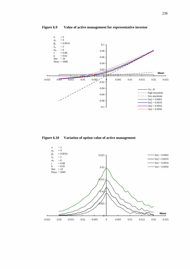
238

Figure 6.9 Value of active management for representative investor

-0.1

-0.08

-0.06

-0.04

-0.02

0

0.02

0.04

0.06

0.08

0.1

-0.025 -0.02 -0.015 -0.01 -0.005 0 0.005 0.01 0.015 0.02 0.025

Mean

Va - Khigh assymtotelow assymtoteSn2 = 0.0002Sn2 = 0.0010Sn2 = 0.0024Sn2 = 0.0050


Figure 6.10 Variation of option value of active management

0

0.005

0.01

0.015

0.02

0.025

-0.025 -0.02 -0.015 -0.01 -0.005 0 0.005 0.01 0.015 0.02 0.025

Mean

Sn2 = 0.0002

Sn2 = 0.0010

Sn2 = 0.0024

Sn2 = 0.0050


239

Figure 6.11 Variation of value with level of sample information

-0.04

-0.02

0

0.02

0.04

0.06

0.08

0.1

0.12

-0.025 -0.02 -0.015 -0.01 -0.005 0 0.005 0.01 0.015 0.02 0.025

Mean

Va - Kn=1n=2n=3n=5n=10

sn2 = 0.0024

ao = 4 bo = 0.0016 lo = 2 mo = 0 r = 0.08 k = 0.02 Hor = 10 Draw = 5000

Figure 6.12 Option value versus level of sample information

-0.002

0

0.002

0.004

0.006

0.008

0.01

0.012

0.014

0.016

0.018

-0.025 -0.02 -0.015 -0.01 -0.005 0 0.005 0.01 0.015 0.02 0.025

Mean

n=1

n=2

n=3

n=5

n=10

sn2 = 0.0024

ao = 4 bo = 0.0016 lo = 2 mo = 0 r = 0.08 k = 0.02 Hor = 10 Draw = 5000

240

Figure 6.13 High uncertainty over value of mm

-0.1

-0.08

-0.06

-0.04

-0.02

0

0.02

0.04

0.06

0.08

0.1

0.12

-0.025 -0.02 -0.015 -0.01 -0.005 0 0.005 0.01 0.015 0.02 0.025

Mean

Va - K

high assymtote

low assymtote

Sn2 = 0.0002

Sn2 = 0.0010

Sn2 = 0.0024

Sn2 = 0.0050


Figure 6.14 Low uncertainty over the value of mm

-0.1

-0.08

-0.06

-0.04

-0.02

0

0.02

0.04

0.06

0.08

0.1

-0.025 -0.02 -0.015 -0.01 -0.005 0 0.005 0.01 0.015 0.02 0.025

Mean



241

Figure 6.15 Strong prior information

-0.15

-0.1

-0.05

0

0.05

0.1

0.15

-0.025 -0.02 -0.015 -0.01 -0.005 0 0.005 0.01 0.015 0.02 0.025

Mean



Figure 6.16 Weak prior information

-0.08

-0.06

-0.04

-0.02

0

0.02

0.04

0.06

0.08

-0.025 -0.02 -0.015 -0.01 -0.005 0 0.005 0.01 0.015 0.02 0.025

Mean



242

Figure 6.17 High cost of changing manager

-0.1

-0.08

-0.06

-0.04

-0.02

0

0.02

0.04

0.06

0.08

0.1

-0.025 -0.02 -0.015 -0.01 -0.005 0 0.005 0.01 0.015 0.02 0.025

Mean



Figure 6.18 Low cost of changing manager

-0.1

-0.08

-0.06

-0.04

-0.02

0

0.02

0.04

0.06

0.08

0.1

-0.025 -0.02 -0.015 -0.01 -0.005 0 0.005 0.01 0.015 0.02 0.025

Mean



243

Figure 6.19 High risk free rate

-0.15

-0.1

-0.05

0

0.05

0.1

0.15

-0.025 -0.02 -0.015 -0.01 -0.005 0 0.005 0.01 0.015 0.02 0.025

Mean

Va - K

high assymtote

low assymtote

Sn2 = 0.0002

Sn2 = 0.0010

Sn2 = 0.0024

Sn2 = 0.0050


Figure 6.20 Low risk free rate

-0.15

-0.1

-0.05

0

0.05

0.1

0.15

-0.025 -0.02 -0.015 -0.01 -0.005 0 0.005 0.01 0.015 0.02 0.025

Mean

Va - K

high assymtote

low assymtote

Sn2 = 0.0002

Sn2 = 0.0010

Sn2 = 0.0024

Sn2 = 0.0050


244

6.6 Testable implications and future research

The model of investors hiring and firing decisions that is presented here has a

number of testable implications. It is my intention to confront a subset of these

implications of the model with UK pension fund data in future research.

Implication 1 Other things equal, investors will more highly value investment

managers that have shorter observable investment histories because investors’

valuation of active management is increasing in uncertainty over the value of µ.

Therefore, other things equal, more money will flow to managers with shorter

observable investment histories. Further, we can expect to see that, of the pension

fund managers which are dismissed by trustee boards, managers with shorter

observable investment histories sustain lower levels of performance before being

dismissed. These implications could be tested using pension fund or mutual fund

data. Both sources are available in the US and the UK.

The first implication requires an estimation of a model of the flows of new money to

fund managers. In that estimation one of the explanatory variables would be the age

of the fund, or another proxy for the level of investors’ prior uncertainty over the

-to-benchmark return distribution. The discussion of

the literature on the strengths and weaknesses of existing fund manager performance-

flow studies can guide the design of the model of portfolio flows. The second

implication, regarding the level of performance preceding dismissal, can be tested

directly by regression of performance at dismissal on the proxy for uncertainty over

the mean of excess-to-benchmark returns. Lunde, Timmermann and Blake (1998)

investigate the hazard function of mutual funds using semi-parametric technique.

Implication 2 The sample mean of the manager’s excess return at the date of

dismissal will be decreasing in sample variance because Vn is increasing in sn2. This

implication is the sample data version of the second of the implications above.

Again a direct test from pension fund data should be feasible.

245

Implication 3 Other things equal, the volume of money managed by managers

which impose low costs of changing manager will be higher. The observable costs

of changing manager would include redemption charges of mutual funds. Data on

the charges of UK unit trusts and US mutual funds is available. The test involves

estimating a model of the asset size of different unit trusts. In that model one of the

explanatory variables is level of entry and exit charges.

Implication 4 The sample mean of the manager’s excess return at the date of

dismissal will be decreasing in the cost of changing manager. In this case, different

asset classes might proxy for the cost of changing manager. The portfolio changes

arising from a change in small capitalisation stock manager will create larger

transaction costs than the portfolio changes associated with a change of large

capitalisation stock manager.

Implication 5 The proportion of new funds that flow to passive managers will be

increasing in the level of the riskless rate of interest and decreasing in the costs of

changing managers. These implications can be tested cross-sectionally and across

time using UK unit trust or US mutual fund data.

6.7 Concluding remarks on the hiring and firing model

The model of hiring and firing of pension fund managers and the associated

simulation study are motivated by a desire to understand how the decisions of

investors, regarding which fund manager to choose and whether to retain that

manager, affect the equilibrium in asset markets. Investors’ decisions on dismissal

can help us to understand the downside risk that fund managers face from poor

portfolio performance results. As argued in chapter 2, an understanding of fund

manager incentives is crucial in studying the market equilibrium.

Empirical studies find that significant poor under-performance by fund managers

may be sustained before the volume of funds under management decreases

substantially. In the model presented here, that observation is explained by the

positive value of the option to delay the decision to dismiss the manager.

246

In the two period model, the value of active management can be broken down into

four components, one of which is the option to decide next period, rather than this

period, whether to dismiss the manager. The simulation of the value of active

management to an investor with an investment horizon of 10 periods shows that this

option value is not trivial. The simulation draws out the crucial role of the level of

uncertainty over the expected value of the manager’s excess return distribution. In

the simulation the difference between a high prior level of uncertainty and a low

prior level is nearly 500 basis points in the value of the manager, and 110 basis

points in the sample mean of excess-to-benchmark returns before the manager is

dismissed. For a longer horizon these values would be commensurately larger.

This level of uncertainty over µ is also increasing in the sample variance of excess-

to-benchmark returns, which has implications for the incentives of fund managers

who are approaching performance levels at which investors are considering

dismissal.

The model highlights the role of the cost of changing manager in the decisions of

investors. The simulation shows the value of active management decreasing in the

cost of changing managers with a sensitivity of less than one. The model also

potentially provides insights into the role of the cost of changing manager in the

balance between the total volume of funds under active versus passive management.

Individual managers who have performed poorly do not have the same incentives as

highly performed managers to minimise the costs to their investors of changing

manager. Since the value of active management, unlike passive management, is

decreasing in the cost of changing manager, there is a negative externality associated

with these costs.

247

Chapter 7 Concluding Remarks

This thesis is concerned with the decisions of private investors and institutional fund

managers. It is contended here that private and institutional investors are

fundamentally different in at least one way – they face different incentives. Further,

that we expect the decisions taken by private and institutional investors to reflect this

difference. In turn, we expect the difference in those decisions to be reflected in

financial market outcomes. The research presented here demonstrates that the

differences in the decisions of private investors and fund managers are substantial

and explain outcomes observed in financial markets.

The organising principle for this study of the decisions of investors and their fund

managers is the familiar starting point of all microeconomic analysis - the

maximisation problem faced by economic agents. In the rise of delegated portfolio

management essay, the questions are: how large is delegated portfolio management?;

how did the rise of institutional fund management come about?; what do we know

about the differences between the incentives, and hence optimisation problems, faced

by private investors and fund managers?; and what can be explained by studying

these differences?

In the accuracy of herding measures essay, the questions proceed from the view that

the differences in incentives are important: if we believe that private investors and

institutional investors form two groups that are fundamentally different in their

trading, then how do we test that belief? A body of empirical literature finds that

fund managers form a herd separate to the rest of the market (private investors), but

how do we know that the measures of herding are accurate? More generally, how do

we test whether any particular measure which is derived from portfolio holdings is

accurate; and can we generalise the findings of studies of herding by US fund

managers to the behaviour of managers in other comparable markets?

The hiring and firing of fund managers essay, is motivated by unanswered questions

about investors’ decisions and fund managers’ incentives: how can the portfolio

performance of managers who are fired be characterised?; what does the attrition rule

mean for the downside of the incentive schedule faced by fund managers?; what is it

248

that makes investors choose to delegate portfolio management when the average

manager under-performs obtainable market indexes?; and how do the hiring and

firing decisions of investors aggregate to create observed dynamics in the investment

management industry?

The contribution of the first essay is an analysis of the significance of the transfer of

control of a large part of the financial asset market from households to institutional

investors. The first point addressed is the scale of the transfer of financial assets

from households to professionally managed portfolios. It is important to bring out in

clear terms what a massive change has occurred in the control of assets and financial

intermediation in the US and UK. The figures themselves beg the question ‘what

does this mean for financial markets?’

Once the data is presented it becomes clear what is driving the shift to delegated

portfolio management in the US, the growth in pension money managed by

institutional investors. The transition of household ownership of US equities from 69

percent of the market in 1969 to 41 percent at year end 1998 is explained largely by

three structural ownership changes. State and local government employee funds

have taken their holding of US equities from near zero to over 10 percent of the

market as their assets grew to 28 percent of GDP and their US equity allocation grew

to 62 percent, between 1967 and 1998. Private pension fund holdings have increased

from 6 to 14 percent of the US equity market in the same period. US mutual funds

held 4 percent of the US equity market in 1983, 7 percent in 1990 and 16 percent in

1998.

For researchers of financial asset markets, the historical perspective of the rise of

portfolio management is important. If the level of institutional ownership affects

market outcomes then it should be recognised that important empirical finance

studies span the period in which the level of institutional ownership is changing

rapidly. As far as I can tell, the possible mis-specification of these studies has not

been recognised elsewhere.

The first essay then analyses what is known and not known about fund manager

incentives. The papers that relate to fund manager incentives are first identified from

249

disparate parts of the literature. Some evidence is drawn from studies that address

psychological issues of rationality, cognitive dissonance and reaction to quality

shocks, but nonetheless provide analysis of the flow of funds to managers. The

conflicting results from the studies of funds flows are subjected to two tests. Firstly,

that the econometrics of the study is sound and secondly, that the results make sense

in the framework of the fund manager’s optimisation problem. This is a crucial step

for the thesis. This analysis characterises what is known about fund manager

incentives.

The incentive schedule of a fund manager relates end of period wealth, or firm value,

to fund rank or the excess-to-benchmark return of the manager. The schedule is

convex in out-performance and concave in under-performance. The schedule shows

that there is little gain to portfolio performance that is only slightly better than that of

peer fund managers. The rewards of new money flow to managers with the highest

return ranking. The schedule is not symmetric in that funds can have poor

performance and not lose much money. The relationship between end of period

wealth (y axis) and relative portfolio performance (x axis) is not as concave in poor

performance as it is convex in high performance.

The incentive schedule of a private investor is a linear relationship between portfolio

total return, or excess-to-benchmark return, and end of period wealth. Therein lies

the essential difference between the incentives of private investors and fund

managers. There are two immediate implications of this difference that can be

understood in terms of the incentive schedule. Firstly, assume that a fund manager

wishes to maximise the expected utility of wealth E[u(wrpt-rmt)] . The expectation

operator is linear, the utility function of wealth is concave and wealth is convex in

positive excess return and concave in negative excess return.74

Under these circumstances fund managers will value assets with positive skewness.75

The testable implications of this conjecture are manifold and can form the basis of

74 This statement is a simplification because the location of the inflexion point of the schedule depends

upon past performance of the fund.

75 In fact managers will have a preference for all positive values of all the odd moments, 1st, 3rd, 5th,….

250

ongoing research. For example we should expect to see fund managers’ holdings of

assets with positive skewness to be greater than that of private investors. Such assets

would include initial public offering stocks and deeply out of the money options.

The second implication of the nature of the incentive schedule is as follows. Assume

that the end of period wealth of a fund manager is a function of excess return over a

window of say three years. Then each year the performance of four years ago drops

out and last year’s performance is inserted. That change in the window shifts the

schedule to the left or the right. That shift leads to a new optimal portfolio. This is a

form of dynamic hedging which may have profound implications. For instance, say

one manager owns none of stock A that is 2 percent of the index and another

manager holds 4 percent of the stock and the stock goes up 150 percent. The

dynamic hedging response will not be symmetric. As the stock rises the manager

who is short versus the market will be induced to buy but the other manager may also

be induced to buy. The relationship between such asymmetric hedging and serial

correlation in stock prices can be investigated in future research.

A testable implication of the conjecture that private investors and fund managers

have substantially different incentives is that, as groups, they will hold significantly

different aggregate portfolios. As they change those portfolios in response to

changes in variables that affect the two differently, we should expect to see net trade

between them which appears as herding by the groups.

Previous studies provide evidence of herding by mutual fund managers and pension

fund managers in the US. But the measures employed in those studies are founded

on assumptions that are invalid but crucial for the accuracy of the measures. This

problem is not unique to measures of herding. Unfortunately, it is standard practice

in much of empirical finance, and especially investment management studies, to

devise a metric and then simply assume that the metric will return a value of zero in

the absence of the phenomenon being measured. Yet, in most of these studies

researchers could simulate datasets, in which the phenomenon is absent, to

empirically estimate the sampling distribution of the metric under null conditions.

251

An alternative to testing the existing herding measures is to devise a new measure of

herding. The testing approach was chosen for two reasons. Firstly, tests of the

accuracy of the extant measures can help determine whether existing empirical

studies of herding are soundly based. Secondly, the attempt to create measures of

herding that encompass all the phenomena that are considered to be herding is part of

the problem with herding measures. That approach has led to measures that do not

have well defined alternative hypotheses. A much better approach is to identify

separate testable predictions for each of the theoretical explanations of herding and

then devise separate tests for each prediction. This is the approach that shall be taken

in ongoing research on fund manager herding.

The contribution of this essay can be summarised as follows. Firstly, the

mathematical description of different types of herding is defined and it is shown that

the major explanations of herding all arise from the same source - fund managers

solve similar optimisation problems. The analysis of explanations of herding in an

optimisation framework presented here hopefully will help to clarify the discussion

of herding.

Secondly, a methodology is developed for estimating the sampling distribution of

any metric which is derived from portfolio holdings data. Researchers can employ a

version of this methodology to test the accuracy of a metric on any portfolio holdings

dataset. There is no need to simply assume that a metric is well calculated. Thirdly,

the accuracy of the existing measures of herding is tested, and the types of stocks for

which these measures are inaccurate, in the UK dataset, are identified. It is found

that the LSV measure overstates the level of herding in small capitalisation stocks

and stocks traded by a small number of managers as a result of the invalid short sales

assumption. The Wermers measure of herding is found to be substantially mis-

specified. The caveats associated with this general test of the model should be

reiterated here. We cannot be sure that the all herding was eliminated in re-sampling

procedure of the test. The re-sampled datasets do not maintain all the essential

characteristics of the actual dataset and the number of re-sampled datasets is finite.

Finally, the existing measures are adjusted for estimated inaccuracy and a significant

level of herding among UK equity unit trust managers is recorded. The level of

252

herding found is commensurate with 14 managers buying or 12 managers selling

where 20 managers trade a stock during a period.76 A large amount of herding by

UK unit trust managers in the smallest market capitalisation stocks is found.

Curiously, that herding is almost entirely herding in buying of the small stocks.

It is difficult to judge the economic significance of these figures. For two reasons we

should not expect to observe ratios of managers trading in the same direction that

approach unity. Firstly, the household sector in the UK holds only 22 percent of the

UK equity market. Therefore the household sector cannot absorb a great deal of

correlated trading from managers. Secondly, if fund managers herd in their trading

of a stock then resultant trading pressure will move the price in the direction that

weakens the force which originally created the herding. For instance, if a large

number of managers buy in concert because they observe a manager who is

perceived to be informed buying the stock, then we can expect the price of the stock

to rise, which in turn induces some managers to sell.

Ongoing research in herding can take two directions. The first, as previously

mentioned, is to identify separate testable predictions from the major theoretical

explanations of herding and test them. A test of the correlated information theory of

herding is afforded by the overlapping nature of the UK unit trust dataset. Fund

managers who report in the January-July cycle overlap managers in the February-

August cycle by five months and managers in the March-September cycle by four

months and so on. By the correlated information hypothesis, the smaller the overlap

period between funds, the less the herding that should be found between them.

Preliminary tests show that the UK portfolio holdings data does support the

correlated trading explanation of herding.

The hiring and firing essay presents results that have the pleasing quality of being

unanticipated when the study began. The first motivation for the study was a need to

better understand the process by which investors decide when to dismiss a poor

performing manager and then which alternative manager to choose. The intention

was to better understand the downside risk faced by managers, by modelling the

76 The difference arises because in the absence of herding, on average 11.6 managers would buy.

253

events leading up to dismissal. Further, to understand aspects of the structure of the

investment management industry, such as the balance between active and passive

management and the concentration of pension fund mandates with only a few of the

largest managers, by studying the hiring and firing decisions of individual investors.

The hiring and firing essay of chapters 5 and 6 contributes to the understanding of

these questions and addresses other questions which were not part of the original

motivation. The principle contributions are twofold. Firstly, to recognise that the

investor has a sequence of real options to delay the project of firing the manager.

Secondly, to understand the dynamic programming nature of the investor’s hiring

and firing decision.

The value of the real option explains some investor behaviour that otherwise seems

incongruous. It partially explains observations of empirical studies of funds flows

that were reviewed in the rise of delegated portfolio management essay. Ippolito

(1992), Goetzmann and Peles (1997) and Sirri and Tufano (1998) find that investor

reaction to poor portfolio performance does not mirror their reaction to high returns.

In many instances investors do not leave poor performing funds at a great rate. This

observation is explained in part by the omission of the worst performing funds from

datasets because they merge with other funds. Another explanation is that investors

are trapped by the high cost of changing manager, including the cost of realising

capital gains. The additional cost recognised in the hiring and firing essay is the cost

of relinquishing the option to delay the costly project of changing manager until the

arrival of information that reduces uncertainty over the decision.

The real option also partially explains the observation of Ippolito (1992) and

Chevalier and Ellison (1997a) that, after controlling for size and portfolio

performance, more money flows to a fund with a two year history than a fund with a

ten year track record. For the two year manager, other things equal, waiting one

more period before deciding on dismissal resolves more uncertainty about the

manager’s ability. Therefore the option to wait is more valuable. The greater

uncertainty in the posterior distribution over the mean of the excess-to-benchmark

return distribution of the two year manager gives the real option associated with that

manager a higher value.

254

The dynamic programming nature of the investor’s problem comes about because the

investor must choose another manager if the current manager is fired. This gives the

model the real world property that the investor expects to hire a sequence of

managers over time. Then we have the result that an investor may choose active

management even when the investor’s prior expectation is that the mean of the

chosen manager’s excess return distribution is negative. The intuition here is that if

an investor on average holds on to good managers for longer than bad managers, then

even if the average manager’s average return is negative, the investor’s time

weighted return can be positive. Therefore, the model partially explains why

investors choose active management when studies show that the average manager

under-performs the market index.

The next step in the study of investors’ hiring and firing decisions is to draw out the

testable implications of the hiring and firing model and confront them with a real

dataset of these decisions.

In the most general terms, this thesis has sought to document the rise of delegated

portfolio management and analyse the significance of this structural change in

financial markets; examine evidence of whether private investors and institutional

investors really are fundamentally different in their trading behaviour; and finally go

to the point of contact between investors and fund managers and investigate the

nature of investor choice decisions and its meaning for fund manager incentives and

market outcomes. The results of this research have, hopefully, progressed the

understanding of the significance of the differences in incentives faced by private

investors and fund managers.

255

References

Ackert, Lucy F., George Athanassakos, June 1998, Institutional Investors, Analyst Following, and the January Anomaly, Working paper.

Admati Anat R., Sudipto Bhattacharya, Paul Pfleiderer, Stephen A. Ross, and Robert E. Verrecchia, 1986, On timing and selectivity, The Journal of Finance 41, 715-732.

Ahluwalia, Manraj, 1995, Fund managers begin to come clean, Benefits and Compensation International 24, April, 9.

Ashton, D. J., 1996, The power of tests of fund manager performance, Journal of Business, Finance and Accounting 23, 1-11.

Avery, Christopher, and Peter Zemsky, Sept. 1998, Multidimensional Uncertainty and Herd Behavior in Financial Markets, The American Economic Review 4, 724-478.

Badrinath S. G., Jayant R. Kale, and Thomas H. Noe, 1995, Of shepherds, sheep, and the cross-autocorrelations in equity returns, The Review of Financial Studies 8, 401-430

Banerjee, Abhijit V., 1992, A simple model of herd behavior, Quarterly Journal of Economics 107, 797-817.

Basu, S., 1977, Investment performance of common stocks in relation to their price earnings ratio: A test of the efficient market hypothesis, The Journal of Finance 32, 663-682.

Berger, James O., 1980, Statistical Decision Theory and Bayesian Analysis, (Spinger-Verlag, New York).

Berkowitz, M. K., and Y. Kotowitz, 1993, Incentives and efficiency in the market for managerial services: A study of Canadian mutual funds, Canadian Journal of Economics 26-4 , 850-866.

Bhattacharya, Sudipto, and Paul Pfleiderer, 1985, Delegated portfolio management, Journal of Economic Theory 36, 1-25.

Bicksler, James L., Andrew H. Chen, and Guilford C. Babcock, 1985, The integration of insurance and taxes in corporate pension strategy, The Journal of Finance 40, 943-957.

Bikhchandani, Sushil, David Hirshleifer, and Ivo Welch, 1992, A theory of fads, fashion, custom and cultural change as informational cascades, Journal of Political Economy 100, 992-1026.

Bildersee, John, and Nathan Kahn, 1987, A preliminary test of the presence of window dressing: Evidence from institutional stock trading, Journal of Accounting, Auditing and Finance 2, 239-265.

Black, Fischer, 1980, The tax consequences of a long run pension policy, Financial Analysts Journal 36, 21-28.

Black, Fischer, 1986, Noise, The Journal of Finance 41, 529-543.

Blake, David, 1992, Modelling Pension Fund Investment Behaviour (Routledge Press, London).

Blake, David, 1996, Pension schemes as options on pension fund assets: Implications for pension fund management, Birkbeck College Discussion Paper PI-9606.

Blake, David, and Alan Timmermann, 1999, Mutual fund performance: Evidence from the UK, Birkbeck College Discussion Paper PI-9903.

256

Blake, David, Bruce Lehmann, and Alan Timmermann, 1999, Asset allocation dynamics and pension fund performance, Birkbeck College Discussion Paper PI-9902.

Bodie, Zvi, Alan J. Marcus, and Robert C. Merton, 1987, Defined benefit versus defined contribution pension plans: What are the real trade-offs? In Issues in Pension Economics, eds. Zvi Bodie and John B. Shoven (University of Chicago Press, Chicago).

Bodie, Zvi, Jay O. Light, Randall Morck, and Robert A. Taggart Jr., 1987, In Funding and Asset Allocation in Corporate Pension Plans: An Empirical Investigation, In Issues in Pension Economics, eds. Zvi Bodie and John B. Shoven (University of Chicago Press, Chicago).

Brealey, Richard A., and Stewart D. Hodges, 1972, Portfolio selection in a dynamic and uncertain world, Financial Analysts Journal 28, 58-69.

Breeden, Douglas, 1979, An intertemporal asset pricing model with stochastic consumption and investment opportunities, Journal of Financial Economics 7, 265-296.

Brennan, Michael J., 1990, Latent assets, The Journal of Finance 45, 709-730.

Brennan, Michael J., 1993, Agency and asset pricing, London Business School, Working paper.

Brennan, Michael J., and Tarun Chordia, 1993, Brokerage commission schedules, The Journal of Finance 48, 1379-1402.

Brinson, Gary P., L. Randolph Hood, and Gilbert L. Beebower, 1986, Determinants of portfolio performance, Financial Analysts Journal 42, 39-44.

Brown Gavin., Paul Draper, and Eddie McKenzie, 1997, Consistency of UK pension fund investment performance, Journal of Business Finance and Accounting 24, 155-178.

Brown, Gavin, Dick Davies, and Paul Draper, 1992a, Pension fund trustees and performance measurement, Management Accounting 7, 38-44.

Brown, Gavin, Dick Davies, and Paul Draper, 1992b, Setting performance measurement objectives for pension funds, Management Accounting 8, 38-40.

Brown, Keith C., W. V. Harlow, and Laura T. Starks, 1996, Of tournaments and temptations: An analysis of managerial incentives in the mutual fund industry, The Journal of Finance 51, 85-110.

Brown, Stephen J., and William N. Goetzmann, 1994, Attrition and mutual fund performance, Presentation to the 1994 American Finance Association meeting.

Brown, Stephen J., and William N. Goetzmann, 1997, Mutual fund styles, Journal of Financial Economics 43, 373-399.

Brown, Stephen J., William N. Goetzmann, Roger G. Ibbotson, and Stephen A. Ross, 1992, Survivorship bias in performance studies, Review of Financial Studies 5, 553-580.

Browne, Sid, 1998, Beating a moving target: Optimal portfolio strategies for outperforming a stochastic benchmark, Columbia University, Working paper.

Bulow, Jeremy I., 1982, What are corporate pension liabilities?, The Quarterly Journal of Economics August, 435-452.

Bulow, Jeremy I., and Myron S. Scholes, 1983, Who owns the assets in a defined benefit pension plan? In Financial Aspects of the US Pension System, eds. Zvi Bodie and John B. Shoven (University of Chicago Press, Chicago).

257

Bulow, Jeremy I., Randall Morck, and Lawrence Summers, 1987, How does the market value unfunded pension liabilities?, In Issues in Pension Economics, eds. Zvi Bodie and John B. Shoven (University of Chicago Press, Chicago).

Busse, Jeffrey A., 1998, Another Look at Mutual Fund Tournaments, Emory University, Working paper.

Capon, Noel, Gavan J. Fitzsimmons, and Russ A. Prince, 1996, An individual level analysis of the mutual fund investment decision, Journal of Financial Services Research 10(1), 59-82.

Chance, Don M., and Michael L. Hemler, 1998, The performance of professional timers: Evidence from executing timing strategies, Virginia Tech. Working Paper.

Chevalier, Judith A., and Glenn D. Ellison, 1997a, Risk Taking by Mutual Funds as a Response to Incentives, Journal of Political Economy, 105-6, 1167-1200.

Chevalier, Judith A., and Glenn Ellison, 1997b, Career concerns of mutual fund managers, NBER & MIT, Working paper.

Chevalier, Judith and Glenn Ellison, 1999, Are some mutual fund managers better than others? Cross-sectional patterns in behavior and performance, Journal of Finance, Forthcoming.

Choe, Hyuk, Kho, Bong-Chan, and Stulz, Rene M, 1999, Do foreign investors destabilise stock markets? The Korean experience in 1997, Journal of Financial Economics, Forthcoming.

Chordia, Tarun, 1996, The structure of mutual fund charges, The Journal of Financial Economics 41, 3-39.

Christoffersen, Susan Kerr, 1997, Fee waivers in money market mutual funds, Wharton Business School, Working paper 97-46.

Coggin, T. Daniel, Frank J. Fabozzi, and Shafiqur Rahman, 1993, The investment performance of US equity pension fund managers: An empirical investigation, The Journal of Finance 48, 1039-1055.

Cohen, Randolph B., 1998, Asset allocation decisions of individuals and institutions, Harvard Business School, Working paper.

Collins, Sean, and Phillip Mack, 1997, The optimal amount of assets under management in the mutual fund industry, Financial Analysts Journal, Sep/Oct 67-73.

Colwell, Peter F., 1998, A primer on piecewise parabolic multiple regression analysis via estimations of Chicago CBD land prices, The Journal of Real Estate Finance and Economics 17-1, 87-98.

Connor, Gregory, and Robert A. Korajczyk, 1986, Performance measurement with the arbitrage pricing theory: A new framework for analysis, Journal of Financial Economics 15, 373-394.

Connor, Gregory, and Robert A. Korajczyk, 1986, The attributes, behaviour and performance of US mutual funds, Review of Quantitative Finance and Accounting 1, 5-26.

Copeland, Thomas E., and David Mayers, 1982, The value line enigma (1965-1978): A case study of performance evaluation issues, Journal of Financial Economics 10, 289-321.

Cornell, Bradford, 1979, Asymmetric information and portfolio performance measurement, Journal of Financial Economics 4, 381-390.

Cuny, Charles, Mark Fedenia, and Robert Haugen, 1995, Professional investor re-entry and the January effect, Working paper.

258

Das, Sanjiv R., Rangarajan Sundaram, 1998, On the regulation of fee structures in mutual funds, NBER, Working paper.

Davanzo, Lawrence B., and Stephen L. Nesbitt, 1987, Performance fees for investment management, Financial Analysts Journal, Jan – Feb, 14-20.

DeGroot, Morris H., 1970, Optimal Statistical Decisions (McGraw-Hill, New York).

DeGroot, Morris H., 1989, Probability and Statistics (Addison-Wesley, Reading Massachusetts).

Devenow, Andrea, and Ivo Welch, 1996, Rational herding in financial economics, European Economic Review 40, 603-615.

Dimson, Elroy, and Paul Marsh, 1983, The stability of UK risk measures and the problem of thin trading, The Journal of Finance 38, 753-783.

Dixit, Avinash K., and Robert S. Pindyck, 1994, Investment Under Uncertainty (Princeton University Press, Princeton).

Dow, James, and Gary B. Gorton, 1997, Noise and volume, Journal of Political Economy, July.

Dybvig, Philip H., and Jonathan E. Ingersoll, 1982, Mean-variance theory in complete markets, Journal of Business 55, 233-51.

Dybvig, Philip H., and Stephen A. Ross, 1985a, The analytics of performance measurement using a security market line, The Journal of Finance 40, 401-416.

Dybvig, Philip H., and Stephen A. Ross, 1985b, Differential information and performance measurement using a security market line, The Journal of Finance 40, 383-416.

Eakins, Stan, and Susan Swell, Do institutions window dress? An empirical investigation, Quarterly Journal of Business and Economics Vol 33-2, 69-78.

Eames, Michael J., 1997, Institutional investor and market myopia: Empirical tests, University of Washington, Working paper.

Edelen, Roger M., and Jerold B. Warner, 1999, Why are mutual fund flow and market returns related? Evidence from high-frequency data, Wharton Financial Institutions Working Paper 99-01.

Edwards, Franklin R., Xin Zhang, 1998, Mutual funds and stock and bond market stability, Journal of Financial Services research 13:3, 257-282.

Efron, Bradley, and R. J. Tibshirani, 1993, Introduction to the Bootstrap (Chapman & Hall, New York).

Elton, Edwin J., Martin J. Gruber, and Christopher R. Blake, 1996, The persistence of mutual fund performance, Journal of Business 69, 133-157.

Ennis, Richard M., 1997, The structure of the investment-management industry: Revisiting the new paradigm, Financial Analysts Journal July-August, 6-13.

Falkenstein, Eric G., March 1996, Preferences for stock characteristics as revealed by mutual fund portfolio holdings, The Journal of Finance 51, 111-135.

Fama, Eugene, 1991, Efficient capital markets: II, The Journal of Finance 46, 1575-1617.

Feldstein, Martin S., and Randall Morck, 1983, Pension funding decisions, interest rate assumptions and share prices. In Financial Aspects of the United States Pension System, eds. Zvi Bodie and John B. Shoven (University of Chicago Press, Chicago).

259

Feldstein, Martin S., and Stephanie Seligman, 1981, Pension funding, share prices, and national savings, The Journal of Finance 36, 801-824.

Ferguson, Robert, and Dean Leistikow, 1996, Unearned performance fees, Journal of Business Finance & Accounting Sept, 1033-1042.

Ferris, S., and D. Chance, 1987, The effect of 12b-1 plans on mutual find expense ratios: A note, The Journal of Finance 42, 1077-82.

Ferson, Wayne E., and Rudi W. Schadt, 1996, Measuring fund strategy and performance in changing economic conditions, The Journal of Finance 51, 425-461.

Flow of Funds Accounts, 1999, The Federal Reserve Board of the United States of America, March.

Francis, Jere R., and Sara Ann Reiter, 1987, Determinants of corporate pension funding strategy, Journal of Accounting and Economics 9(1), 35-59.

Friedman, B.M., 1983, Pension funding, pension asset allocation and corporate finance: Evidence from individual company data. In Financial Aspects of the United States Pension System, eds. Zvi Bodie and John B. Shoven (University of Chicago Press, Chicago).

Friend, Irwin, Marshall Blume, and Jean Crockett, 1970, Mutual Funds and Other Institutional Investors (McGraw Hill, New York).

Froot, Kenneth A., David S. Scharfstein, and Jeremy C. Stein, 1992, Herd on the street: Informational inefficiencies in a market with a short term speculation, Journal of Finance 47, 1461-1484.

Fund Management Survey, 1996, Institutional Fund Managers Association (London).

Goetzmann, William N., and Nadav Peles, 1997, Cognitive dissonance and mutual fund investors, The Journal of Financial Research 20(2), 145-158.

Goetzmann, William N., and Roger G. Ibbotson, 1994, Do winners repeat?, Journal of Portfolio Management Winter, 9-18.

Goetzmann, William N., and Stephen J. Brown, 1993, Attrition and mutual fund performance, Leonard Stern School of Business, New York University, Working paper.

Goetzmann, William N., Bruce Greenwald, and Gur Huberman, 1992, Market response to mutual fund performance, Columbia University, Working paper (92-25).

Goetzmann, William N., Jonathan Ingersoll Jr., and Stephen A. Ross, 1997, High water mark, Yale School of Management, Working paper.

Goetzmann, William N., Massimo Massa, 1998, Index funds and stock market growth, Working paper.

Golec, Joseph H., 1988, Do mutual fund managers who use incentive compensation outperform those who don’t?, Financial Analysts Journal Nov/Dec, 75-78.

Golec, Joseph H., 1992, Empirical tests of a principal-agent model of the investor-investment advisor relationship, Journal of Financial and Quantitative Analysis 27(1), 81-95.

Golec, Joseph H., 1996, The effects of mutual fund managers’ characteristics on their portfolio performance, risk and fees, Financial Services Review 5-2, 133-148.

Gompers, Paul A., and Andrew Metrick, 1998, Are the hundred-million-dollar managers just like everyone else? An analysis of stock ownership, concentration, and trading by large institutions, HBS and NBER, Working paper.

260

Gompers, Paul A., and Josh Lerner, 1997, Venture capital fundraising, firm performance, and the capital gains tax, Harvard University, Working paper.

Gompers, Paul, and Josh Lerner, 1995, An analysis of compensation in US venture capital partnerships, Harvard Business School, Working paper (95-009).

Goode, Prof. Roy (Chairman), September 1993, Pension Law Reform Volume 1, The Report of the Pension Law Review Committee (HMSO, London).

Greene, William H., 1990, Econometric Analysis (MacMillan, New York).

Grinblatt, Mark S., and Sheridan Titman, 1988, The evaluation of mutual fund performance: An analysis of monthly returns, Anderson Graduate School of Management, UCLA, Working paper (13-86).

Grinblatt, Mark S., and Sheridan Titman, 1989a, Adverse risk incentives and the design of performance-based contracts, Management Science 35(7), 807-822.

Grinblatt, Mark S., and Sheridan Titman, 1989b, Mutual fund performance: An analysis of quarterly portfolio holdings, Journal of Business 62(3), 393-416.

Grinblatt, Mark S., and Sheridan Titman, 1992, The persistence of mutual fund performance, The Journal of Finance 47, 1977-1984.

Grinblatt, Mark S., and Sheridan Titman, 1993, Performance measurement without benchmarks: An examination of mutual fund returns, Journal of Business 66, 47-68.

Grinblatt, Mark S., and Sheridan Titman, 1994, A study of monthly mutual fund returns and performance evaluation techniques, Journal of Financial and Quantitative Analysis 29, 419-444.

Grinblatt, Mark S., Sheridan Titman, and Russell Wermers, 1995, Momentum investment strategies, portfolio performance and herding: A study of mutual fund behavior, The American Economic Review 85, 1088-1105.

Grinold, Richard, and Andrew Rudd, 1987, Incentive fees: Who wins? who loses?, The Financial Analysts Journal, Jan-Feb, 27-38.

Grossman, Sanford J., 1976, On the efficiency of competitive stock markets when trades have diverse information, The Journal of Finance 31, 573-585.

Grossman, Sanford J., and Stiglitz Joseph E., 1980, On the impossibility of informationally efficient markets, The American Economic Review 70, 393-408.

Grossman, Sanford J., and Zhongquan Zhou, 1996, Equilibrium analysis of portfolio insurance, The Journal of Finance 51, 1379-1403.

Gruber, Martin J., 1996, Another puzzle: The growth in actively managed mutual funds, The Journal of Finance 51, 783-810.

Gumbel, Alexander, June 1998, Herding in Delegated Portfolio Management: When is Comparative Performance Information Desirable?, Journal of Economic Literature.

Halpern, Philip, and Isabelle I. Fowler, 1991, Investment management fees and determinants of pricing structure in the industry, Journal of Portfolio Management 17(2), 74-79.

Harrison, Michael J., and William F. Sharpe, 1983, Optimal funding and asset allocation rules for defined benefit pension plans. In Financial Aspects of the United States Pension System, eds. Zvi Bodie and John B. Shoven (University of Chicago Press, Chicago).

261

Heinkel, R., and N.M. Stoughton, 1994, The dynamics of portfolio management contracts, Review of Financial Studies 7, 351-387.

Hendricks, Daryll, Jayendu Patel, and Richard Zeckhauser, 1993, Hot hands in mutual funds: Short-run persistence of relative performance 1974-1988, The Journal of Finance 48, 93-130.

Hessel, Christopher A., and Morton Norman, Financial characteristics of neglected and institutionally held stocks, Journal of Accounting, Auditing & Finance, 313-330.

Hirshleifer, David, Avanidhar Subrahmanyam, and Sheridan Titman, 1994, Security analysis and trading patterns when some investors receive information before others, The Journal of Finance 49, 1665-1698.

Holmstrom, Bengt, 1979, Moral hazard and observability, The Bell Journal of Economics and Management Science 10, 74-91.

Holmstrom, Bengt, 1982, Managerial incentive problems – a dynamic perspective, in Essays in Economics and Management in Honor of Lars Wahlbeck, Swedish School of Economics, Helsinki.

Horan, Stephen M., 1998, A comparison of indexing and beta among pension and non-pension assets, Journal of Financial Research Vol. 21-3, 255-275.

Horowitz, Joel, 1996, Bootstrap methods for covariance structures, University of Iowa, Working paper.

Hsiao, Cheng, 1986, Analysis of Panel Data (Cambridge University Press, Cambridge).

Huang, Chi-Fu, and Robert H. Litzenberger, 1988, Foundations for Financial Economics (North-Holland, New York).

Huddart, Steven, 1997, Reputation and performance fee effects on portfolio choice by investment advisers, Fuqua School of Business, Duke University, Working paper.

Ingersoll, Jonathon E., 1987, Theory of Financial Decision Making (Rowman and Littlefield, Totowa New Jersey).

Institutional Fund Managers Association, 1996, Fund Management Survey report.

International Monetary Fund, 1994, International Financial Statistics Yearbook.

International Monetary Fund, 1997, International Financial Statistics Yearbook.

International Monetary Fund, September 1997, International Financial Statistics.

Ippolito, Richard A., 1987, Turnovers, fees and pension plan performance, The Financial Analysts Journal, Nov-Dec, 16-26.

Ippolito, Richard A., 1992, Consumer reaction to measures of poor quality: Evidence from the mutual fund industry, Journal of Law and Economics 35, 45-70.

Jagganathan, Ravi, and Robert A. Korajczyk, 1986, Assessing the market timing performance of managed portfolios, Journal of Business 59, 217-235.

Jain, Arvind K., and Satyadev Gupta, 1987, Some evidence on ‘herding’ behavior of US banks, Journal of Money, Credit and Banking 19, 78-89.

Jegadeesh, N., and Sheridan Titman, 1993, Returns to buying winners and selling losers: implications for stock market efficiency, The Journal of Finance 48, 65-91.

262

Jensen, Michael C., 1968, The performance of mutual funds in the period 1945-64, The Journal of Finance 23, 389-416.

Jensen, Michael C., 1969, Risk, the pricing of capital assets, and the evaluation of investment portfolios, Journal of Business 42, 167-247.

Keegan, Jeffrey, 1998, Size, gray hair figure hugely in asset-management M&A deals, Investment Dealers’ Digest July, 21.

Khorana, Ajay, 1996, Top management turnover: An empirical investigation of mutual fund managers, Journal of Financial Economics 40, 403-427.

Kihn, John, 1996, To load or not to load? A study of the marketing and distribution charges of mutual funds, The Financial Analysts Journal 52(3), 28-36.

Klemkosky, Robert C., 1977, The impact and efficiency of institutional net trading imbalances, The Journal of Finance 32, 79-86.

Kodres, Laura E., and Matthew Pritsker, 1995, Directionally similar position taking and herding by large futures markets participants, Working paper.

Kraus, Alan, and Hans Stoll, 1972, Parallel trading by institutional investors, Journal of Financial and Quantitative Analysis 7, 2107-2138.

Kreps, David M., 1990, A Course in Microeconomic Theory (Princeton University, Princeton).

Kritzman, Mark P., 1987, Incentive fees: Some problems and some solutions, Financial Analysts Journal Jan-Feb, 21-26.

Kyle, Albert S., 1985, Continuous auctions and insider trading, Econometrica 53, 1315-1335.

Lakonishok, Josef, Andrei Shleifer, and Robert W. Vishny, 1992a, The impact of institutional trading on stock prices, Journal of Financial Economics 32, 23-43.

Lakonishok, Josef, Andrei Shleifer, and Robert W. Vishny, 1992b, The structure and performance of the money management industry: Comments and discussion, Brookings Papers on Economic Activity, 339-391.

Lakonishok, Josef, Andrei Shleifer, Richard Thaler, and Robert W. Vishny, 1991, Window dressing by pension fund managers, The American Economic Review 81, 227-231.

Lee, S. L., and C.W.R. Ward, 1980, The association of stock market volatility and parallel trading by UK institutional investors, Journal of Business Finance and Accounting 7, 415-425.

Lehmann, Bruce N., and David M. Modest, 1987, Mutual fund performance evaluation: A comparison of benchmarks and benchmark comparisons, The Journal of Finance 42, 233-265.

Leonard, Spring B., and April K. Caudill, 1996, The Mutual Fund Fact Book, (The National Underwriter Company, Cincinnati).

Lettau, Martin, 1997, Explaining the facts with adaptive agents: The case of mutual fund flows, Journal of Economic Dynamics and Control 21, 1117-1147.

Lintner, John, 1965, The valuation of risky assets and the selection of risky investments in stock portfolios and capital budgets, Review of Economics and Statistics February, 13-37.

Litzenberger, Robert H., and Krishna Ramaswamy, 1979, The effect of personal taxes and dividends on capital asset prices: Theory and empirical evidence, Journal of Financial Economics 7, 163-195.

263

Lo, Andrew W., and MacKinlay Craig W., 1990, When are contrarian profits due to stock market overreaction?, Review of Financial Studies 3, 175-206.

Long, John B. Jr, 1978, The market valuation of cash dividends: A case to consider, Journal of Financial Economics 9, 3-18.

Lunde, Asger, Allan Timmerman, and David Blake, 1998, The hazards of mutual fund under performance: A Cox regression analysis, UC San Diego, Working paper.

Maddala, G.S., 1991, Limited Dependent and Qualitative Dependent Variables in Econometrics (Cambridge University Press, Cambridge).

Malliaris, A. G., and Brock W. A., 1991, Stochastic Methods in Economics and Finance, (North-Holland, New York).

Marcus, Alan J., 1983, Corporate pension policy and the value of PBGC insurance, in Financial Aspects of the United States Pension System, eds. Zvi Bodie and John B. Shoven (University of Chicago Press, Chicago).

Maug, Ernst, and Narayan Naik, 1996, Herding and delegated portfolio management: The impact of relative performance evaluation on asset allocation, London Business School, Working paper.

Mayers, David, and Edward M. Rice, 1979, Measuring portfolio performance and the empirical content of asset pricing models, Journal of Financial Economics 7, 3-29.

Merton, Robert C., 1973, An intertemporal capital asset pricing model, Econometrica 41, 867-80.

Michel, Allen, and Israel Shaked, 1986, Industry influence on pension funding, Journal of Portfolio Management 12(3), 71-77.

Modigliani, Franco, and Merton H. Miller, 1958, The cost of capital, corporation finance, and the theory of investment, American Economic Review, June, 261-297

Musto, David K., 1997, Portfolio disclosures and year-end price shifts, Journal of Finance 52-4, 1563-1587.

Musto, David K., 1998, Investment decisions depend on portfolio disclosures, University of Pennsylvania, Working paper.

Musto, David K., Sept. 1997, Portfolio disclosures and year-end price shifts, Journal of Finance 52, 1563-1587.

Mutual Fund Fact Book, 1995 (The Investment Company Institute, New York).



Nanda, Vikram, I. P. Narayanan, and Vincent A. Warther, 1997, Liquidity, investment ability, and mutual fund structure, University of Michigan and University of Chicago, Working paper.

National Association of Pension Funds, 1991, Report of the Committee of Enquiry into Performance Measurement (London).

National Association of Pension Funds, 1996, Annual Survey 1995 (London).

New York Stock Exchange Fact Book, 1996 (New York Stock Exchange, New York).

264

Nobles, R.L., 1985, Conflicts of interests in trustees management of pension funds - An analysis of the legal framework, Industrial Law Journal 14, 1-17.

Nobles, R.L., 1992, The exercise of trustees discretion under a pension scheme, Journal of Business Law May, 261-280.

O’Hagan, Anthony, 1994, Kendall’s Advanced Theory of Statistics, Volume 2B, Bayesian Inference (Halsted Press, New York).

Odean, Terrance, 1998a, Are investors reluctant to realise their losses?, Journal of Finance 53, 1775-1789.

Odean, Terrance, 1998b, Do investors trade too much?, UC Santa Cruz, Working paper.

Office for National Statistics, 1996, UK National Accounts (HMSO, London).

Office for National Statistics, December 1997, Financial Statistics (HMSO, London).

Orphanides, Athanasios, 1996, Compensation incentives and risk taking behavior: Evidence from mutual funds, Board of Governors of the Federal Reserve System, Working paper (96-21).

Orphanides, Athanasios, Brian Reid, and David H. Small, 1994, The empirical properties of a monetary aggregate that adds bond and stock mutual funds to M2, Federal Reserve Bank of St Louis Review 76(6), 31-51.

Papke, Leslie E., 1991, Participation in and contributions to 401(k) pension plans: Evidence from plan data, Journal of Human Resources 30(2), 311-325.

Patel, Jayendu, Richard Zeckhauser, and Darryll Hendricks, 1990, The rationality struggle: Illustrations from financial markets, The American Economic Review 81, 232-236.

Patel, Jayendu, Richard Zeckhauser, and Darryll Hendricks, 1994, Investment flows and performance: Evidence from mutual funds, cross-border investments, and new issues. In Japan, Europe, and International Financial Markets: Analytical and Empirical Perspectives, by Sato, edited by Sato Ryuzo, Richard M. Levich, and Rama V. Ramachandran, 51-72.

Pensions Management, November 1994 (The Pearson Group, London).

Perold, A., and R. Salmon, 1991, The right amount of funds under management, Financial Analysts Journal, May/June.

Petersen, Mitchell A., 1994, Cashflow variability and firms’ pension choice: A role for operating performance, Journal of Financial Economics 36, 361-382.

Poterba, J., 1998, Population age structure and asset returns: an empirical investigation, NBER Working Paper No. 6774.

Poterba, J., S. Venti, and D. Wise, 1992, 401(k) plans and tax deferred saving, National Bureau of Economic Research, Working paper (4181).

Potter, Mark, Sept. 1998, The relationship between aggregate mutual fund flows and security returns, Working paper.

Pound, John, and Robert J. Shiller, 1987, Are institutional investors speculators?, The Journal of Portfolio Management Spring, 46-52.

Record Jr., Eugene E., and Mary Ann Tynan, 1987, Incentive fees: The basic issues, Financial Analysts Journal, Jan/Feb, 39-43.

265

Reinganum, Marc R., 1981, Mis-specification of capital asset pricing: Empirical analysis based on earnings yields and market value, Journal of Financial Economics 9, 19-46.

Remolona, Eli M., Paul Kleinman, Debbie Gruenstein, 1997, Market returns and mutual fund flows, FRBNY Economic Policy Review, July, 33-52.

Rockinger, Michael, 1995, Determinants of capital flows to mutual funds, HEC, Working paper.

Roll, Richard, 1977, A critique of the asset pricing theories tests part 1: On past and potential testability of the theory, Journal of Financial Economics 4, 129-176.

Roll, Richard, 1978, Ambiguity when performance is measured by the securities market line, The Journal of Finance 33, 1051-1069.

Ross, Stephen A., 1973, The economic theory of agency; The principal’s problem, American Economic Review May, 134-39.

Ross, Stephen A., 1976, The arbitrage theory of asset pricing, The Journal of Economic Theory 13, 343-362.

Ross, Stephen A., 1998, Some notes on compensation, agency theory, and the duality of risk aversion and riskiness, Sloan School, Working paper.

Roston, Marc, 1997, Mutual fund managers and life cycle risk: An empirical investigation, Department of Economics, University of Chicago, Working paper.

Santini, Donald L., and Jack W. Aber, 1996, Investor response to mutual fund policy variables, Financial Review 31, 765-786.

Scharfstein, David, and Jeremy C. Stein, 1990, Herd behavior and investment, The American Economic Review 80, 465-479.

Schuller, Tom, and Jeffrey Hyman, 1983, Trust law and trustees: Employee representation in pension schemes, Industrial Law Journal 12, 84-98.

Securities Industry Fact Book, 1996, Securities Industry Association (New York).

Sharpe, William F., 1964, Capital asset prices: A theory of market, equilibrium under conditions of risk, The Journal of Finance, 425-442.

Sharpe, William F., 1976, Corporate pension funding policy, Journal of Financial Economics 3, 183-193.

Shefrin, H., and M. Statman, 1985, The disposition to sell winners too early and ride losers too long: Theory and evidence, Journal of Finance 40 , 777-790.

Shiller, Robert J., and John Pound, 1989, Survey evidence on diffusion of interest and information among investors, Journal of Economic Behaviour and Organisation 12, 47-66.

Shukla, Ravi, and C. Trzcinka, 1992, Performance measurement of managed portfolios, Financial Markets Institutions and Investment 4.

Sias, Richard W., and Starks, Laura T., 1997, Return autocorrelation and institutional investors, Journal of Financial Economics 46, 103-131.

Siggelkow, Nicolaj, 1999, Expense shifting: An empirical study of agency costs in the mutual fund industry, Wharton Working Paper.

266

Sirri, Eric R., and Peter Tufano, 1998, Costly search and mutual fund flows, The Journal of Finance 53, 1589-1622

Smith, Keith V., 1978, Is fund growth related to fund performance?, Journal of Portfolio Management 5, 49-54.

Spitz, A. Edward., 1970, Mutual fund performance and cash inflow, Applied Economics 2, 141-145.

Starks, Laura, 1987, Performance incentive fees: An agency theoretic approach, Journal of Financial and Quantitative Analysis 22, 17-32.

Stokey, Nancy L., and Robert E. Lucas, 1993, Recursive Methods in Economics and Dynamics (Harvard University Press, Cambridge Massachusetts).

Stoughton, Neal, 1994, Moral hazard and the portfolio management problem, The Journal of Finance 48, 2009-28.

Tepper, Irwin, 1981, Taxation and corporate pension policy, The Journal of Finance 36, 1-13.

Titman, Sheridan, July 1989, Adverse risk incentives and the design of performance-based contracts, Management Science Vol. 35-7, 807-822.

Treynor, Jack L., 1961, Toward a theory of the market value of risky assets, Unpublished manuscript.

Treynor, Jack L., 1977, The principles of corporate pension finance, The Journal of Finance 32, 627-638.

Trzcinka, Charles, and R. Zweig, 1990, An economic analysis of the cost and benefits of SEC Rule 12b-1, Monograph Series in Finance and Economics 1990-1, New York University.

Warther, Vincent, 1995, Aggregate mutual fund flows and security returns, Journal of Financial Economics 39(2), 209-235.

Wermers, Russell R., 1995, Herding, trade reversals and cascading by institutional investors, University of Colorado Boulder, Working paper.

Wermers, Russell R., 1999, Mutual fund herding and the impact on stock prices, The Journal of Finance 53, 581-621.

Wharton School of Finance and Commerce, University of Pennsylvania, 1962, A Study of Mutual Funds (US Government Printing Office).

Williamson, J. Peter., 1970, Mutual fund performance and net new money, Unpublished manuscript.

Willinger, G. Lee, 1992, A simulation comparison of actuarial and contingent claims models for funded pension liabilities, Quarterly Journal of Business and Economics 31, 72-97.

Woerheide, Walt, 1982, Investor response to suggested criteria for the selection of mutual funds, Journal of Financial and Quantitative Analysis 17, 129-137.

World Markets Company, 1995, What Herd?, What Median? (WM Research, Edinburgh UK).

Wylie, Samuel V., 1996a, Tests of the accuracy of herding measures using UK data, abstracted in The Journal of Finance 52, 1259.

Wylie, Samuel V., 1996b, Fund Management Survey 1996 (Institutional Fund Managers Association, London).

Wylie, Samuel V., 1997, Performance measurement without benchmarks, Working paper.

267

Yatchew, Adonis, and Zvi Griliches, 1985, Specification errors in probit models, Review of Economics and Statistics 67, 134-139.

Zeckhauser, Richard, Jayendu Patel, and Darryll Hendricks, 1991, Non rational actors and financial market behaviour, Theory and Decision 31, 257-287.

Zheng, Lu, 1999, Is money smart - A study of mutual fund investors fund selection ability, Journal of Finance 54, Forthcoming.

01/27/00

1

Doctoral Dissertation London Business School University of ...

Documents

Transcript of Doctoral Dissertation London Business School University of ...