DO SWITCHING COSTS MAKE MARKETS MORE OR LESS COMPETITIVE?: THE CASE OF 800-NUMBER PORTABILITY*

Abstract

Do switching costs reduce or intensify price competition in markets where firms charge the same price to old and new consumers? The answer is theoretically ambiguous because a firm prefers to charge a higher price to previous purchasers who are “locked-in” and a lower price to unattached consumers who offer higher future profitability. 800-number portability provides empirical evidence to determine whether switching costs reduce or intensify price competition under a single price regime. Before portability, a customer had to change toll-free numbers in order to change service providers. In May 1993, 800-numbers became portable, under a regulatory regime that precluded price discrimination between old and new consumers. I test how AT&T and MCI adjusted their toll-free services prices in response to portability. I find that the firms reduced prices with portability, implying that the switching costs arising from non-portability made the market less competitive. Thus, despite rapid growth in toll-free services, the firms’ incentives to charge a higher price to “locked-in” consumers exceeded their incentive to capture new consumers. Keywords: switching costs, lock-in, number portability, telecommunications JEL Classifications: L13, L96, D43

V. Brian Viard Graduate School of Business, Stanford University

518 Memorial Way Stanford, CA 94305-5015

Tel: 650-736-1098 viard_brian@gsb.stanford.edu

This Draft: 6/23/2003

* I would like to thank Dennis W. Carlton, Judith A. Chevalier, Robert Gertner and Fiona Scott Morton for numerous suggestions. I have also benefited greatly from comments by Lanier Benkard, John Browning, Ann Ducharme, Thomas Hellman, Christopher Knittel, Lars Lefgren, Paul Oyer, Katja Seim, Tomas Serebrisky, Andrzej Skrzypacz, Scott Sherburne, Scott Stern, Alan D. Viard and Rickard E. Wall. I want to thank George David and Bill Goddard of CCMI, a division of UCG, for their time and generosity in making the tariff data available. Steve Shea of TechCaliber, LLC, Bill Clebsch of Stanford University and Mike Dettorre of Deloitte Consulting contributed enormously to my understanding of the telecommunications industry. I would like to acknowledge financial support from the State Farm Companies Foundation and the Fletcher Jones Foundation. All errors are my own.

1

Firms offering products with significant switching costs generally prefer to charge a higher price

to existing customers who are “locked-in” and a lower price to unattached consumers who offer

higher future profitability. However, transactions costs, regulatory constraints or the ability of

customers to arbitrage price differences may prevent firms from charging different prices to new

and existing customers. Nonetheless, the previous empirical switching costs literature has

primarily examined firms engaged in differential pricing. In this paper I take advantage of a

unique situation in which switching costs changed to determine its effect on prices in a single-

price regime. To inform my estimation, I extend previous theoretical models to develop an

estimable empirical model. Models in which firms charge a single price have been limited to

two-period models or models in which switching costs are assumed to be high enough that no

customers switch in equilibrium. I develop an infinite-horizon model that allows for actual

switching in equilibrium.

In the model, an increase in switching costs may lead to either an increase or a decrease in

equilibrium prices. The net effect depends on the relative number of old and new consumers and

the importance of “lock-in” relative to the incentives for attracting new consumers. I test the

effect of switching costs on competition in the high-growth, toll-free services market. To justify

the applicability of the theoretical model, I provide evidence of significant switching in this

market and show that characteristics of prices are consistent with the model’s implications. Since

rapidly growing markets have a greater proportion of new consumers, there is a higher

probability that switching costs will lead to increased price competition. In spite of this rapid

growth, I find that switching costs led to lower competition for toll-free services.

Originally, users of 800-, or toll-free, service could not switch providers without changing their

telephone number. The introduction of portability on May 1, 1993 reduced switching costs at the

same time as regulatory restrictions required firms to charge the same price to new and existing

consumers. Controlling for other factors, declines in price resulting from portability is evidence

that switching costs make markets less competitive, while increases in price would be opposing

evidence.

2

Portability lowered prices for both types of toll-free services I examine, implying that higher

switching costs under non-portability made the market less competitive. First, I use contracts for

AT&T virtual private network (VPN) services, a bundle of long-distance services offered to

large users. Estimating the policy function implied by the theoretical model and taking advantage

of the fact that the data provides actual marginal cost, I find that VPN contracts constrained by

non-portability had significantly higher prices than those unconstrained by non-portability after

controlling for cost. I use contracts that contained no toll-free services as a control group (the

other services were always portable) and find that the prices on these contracts were not

significantly affected by portability. Second, I use prices for stand-alone (unbundled) services

offered by both MCI and AT&T. Again estimating the policy function and controlling for cost, I

find that prices for toll-free services dropped after portability in a manner consistent with higher

prices due to switching costs. Moreover, portability had no significant effect on prices for toll

services (which were always portable).

The magnitude of the effect on the average VPN and stand-alone toll-free users is approximately

the same once I adjust for the fact that toll-free services comprise only a portion of VPN

contracts. I estimate that portability lowered toll-free prices by approximately fourteen percent

for the average consumer. For larger VPN users, the effect is much greater, consistent with large

users being more “locked-in.” I offer evidence that these effects are not due to confounding

events, including AT&T’s loss of monopoly power over vanity numbers and changes in

regulation. The results indicate that AT&T’s and MCI’s incentive to charge higher prices to

existing consumers subject to the high switching costs of non-portability exceeded their

incentive to “capture” new users by charging lower prices. Given the rapid growth in 800

services during this period (AT&T’s toll-free minutes grew over fourteen percent per year),

switching costs are likely to increase prices in single-price markets with lower growth rates.

3

Because it is difficult to measure switching costs, tests of single-price switching costs models are

few.1 Sharpe (1997) tests the Klemperer (1987a) result that prices are more competitive the

greater the consumer turnover in a market. Sharpe finds that the degree of migration into or out

of a local market has a positive effect on bank deposit interest rates paid to depositors. This does

not address the overall effect of switching costs on prices, the question of this paper. Kim, Kliger

and Vale (2001) employ an Euler equation approach to estimate switching costs and probabilities

from aggregated data in a panel data set of Norwegian banks. Their paper provides a

methodology for inferring switching costs levels from price and aggregate share movements

rather than using a change in switching costs to infer its effect on prices as I do. Knittel (1997)

finds that higher fees charged for switching long-distance providers is associated with greater

margins for the long-distance providers. However, the empirical setting does not offer a natural

control group, the role played by toll services in this paper, which makes it difficult to control for

other changes. This is important given the variation in switching costs occurs over time.

In the next section I provide background on the toll-free services industry. Section 2 develops a

theoretical model of switching costs. In Section 3, I describe VPNs and the data. Section 4

describes the econometric tests and empirical results, and I conclude in Section 5.

1. Toll-Free Services and Portability

After the divestiture of AT&T in 1984, other inter-exchange carriers (IXCs) were legally

allowed to provide 800- or toll-free service.2 However, the District Court charged with

overseeing AT&T’s breakup ruled that AT&T retained patent rights over the database

technology that enabled local exchange carriers (LECs) to switch toll-free calls to different

1 Three other studies look at contexts in which firms can price discriminate between old and new consumers (dual-price models). Borenstein (1991) finds that gasoline stations price discriminated against consumers of leaded gasoline to exploit the increased switching costs imposed on these consumers as the stations phased it out in favor of unleaded gasoline. Calem and Mester (1995) test for switching costs in the credit card industry. Elzinga and Mills (1998), using transaction-level data on wholesale cigarettes, show that customers exhibiting characteristics associated with high switching costs are less likely to switch to a new entrant during a price war. 2 The service is often called 800-service because all toll-free numbers originally began with the numbers “800.” Toll-free numbers now also begin with “888,” “877” and “866.”

4

IXCs.3 In 1986, the Federal Communications Commission (FCC) decided, as an interim

measure, that toll-free calls would be routed based on the next three digits after 800 (800-NXX-

YYYY), referred to as NXX screening. The FCC assigned each IXC one or more NXX prefixes

for use in 800-service, and the LECs routed all calls beginning with “800-NXX” to the IXC

assigned that NXX code. Although NXX screening allowed entry, the method imposed

substantial switching costs on toll-free users. Because of the dependence on NXX, a user who

wanted to switch carriers for its toll-free service had to switch numbers. Because firms usually

publish 800-numbers widely, imprinting them on stationery, advertisements and business cards,

the cost of changing numbers is significant.4

The FCC required the LECs to install a new switching system on May 1, 1993, a byproduct of

which was that it allowed them to assign and route any 800-call to any IXC.5 Users were now

able to switch providers without changing their phone number. Switching costs did not drop to

zero after portability – there were still costs of renegotiating a contract, running a redundant

parallel system during the transition and relationship-specific costs. Nonetheless, switching costs

were much lower than under non-portability. Most popular articles published prior to portability

speculated that portability would lower prices for toll-free services.6 This view has prevailed in

academic articles published since portability. Both Ward (1993) and MacAvoy (1995) cite

portability as a reason to expect more competition for 800-services. Despite these references, no

academic studies have rigorously analyzed the effect of portability on price competition.

Since comprehensive data on switching by toll-free customers is not available, I gathered

evidence of whether non-portability precluded switching altogether. I identified all firms with

3 The difficulty in switching toll-free calls was that the recipient of the calls pays so that the LEC could not simply route the call to the initiator’s chosen long-distance provider. 4 For statements in the popular press describing these switching costs, see: “Carriers Plot Strategies at Dawn of War Over 800 Users” (Network World, November 9, 1992), “Firm Predicts Savings With Tariff 12 Net” (Network World, February 12, 1990), “Net Users Remaining Loyal After AT&T’s Recent Outage” (Network World, January 29, 1990), Telecommunications Market Sourcebook (Frost & Sullivan, 1995). 5 As I explain below, portability was not the primary intent of the new switching technology. 6 See “Portability Sparks Price Wars” (Catalog Age, May 1993), “Airlines + Price Wars = Big 800 Traffic” (800-900 Review, Strategic Telemedia, May 1, 1992), “Portability Adds Fuel to 800 Fire” (Karen Burka, Catalog Age, October, 1992).

5

sales over five million dollars in successive editions of The Directory of Mail Order Catalogs

and traced the ownership of their 800-numbers over time based on NXX codes. I focused on only

the largest mail-order firms since they were most affected by non-portability. As Table 1 shows,

a significant percentage of customers of the later entrants (MCI and Sprint) switched from

AT&T, although the sample size is admittedly small. The fact that no users switched to AT&T is

reasonable given the small sample size and the fact that fewer consumers would switch to a long-

established incumbent.

I cannot perform this analysis post-portability because NXX codes no longer map to specific

carriers and no comprehensive toll-free directories are available. I have to rely on (potentially

biased) reports of significant switching made by the IXCs themselves.7 This evidence of

switching pre- and post-portability dictates a theoretical model that allows for equilibrium

switching.

Switching costs can lower prices in a dynamic setting only if the number of new consumers is

sufficiently large relative to the number of old consumers. The data indicate that toll-free

minutes grew almost nine-fold from 1985 to 1999. This measure does not reveal whether new or

old consumers generated this growth, but the growth rate is sufficiently high that decreased

competitiveness resulting from switching costs is plausible.

2. Theoretical Model

The primary purpose of the theoretical model is to provide a basis for empirical estimation, a

policy equation that I can estimate. Given this, I focus only on results relevant for my empirical

application rather than comprehensive analysis. The secondary purpose is to show, in a model

that accurately reflects the empirical setting, that when firms are constrained to charge a single

7 AT&T claimed that 10,000 users representing over $140 million in revenue switched their numbers to its service, while MCI claimed 6,550 users representing over $170 million and Sprint “several thousand” customers. (“Winds of Change Sweeping Over Cooped-Up 800 World,” Network World, May 3, 1993). AT&T also claimed that it had retained 505 out of 531 users of and MCI claimed it had gained $500 million in new commitments (not annualized) for VPN services since portability. (“AT&T & MCI Report ‘Fresh Look’ Results,” Internet Week, August 9, 1993).

6

price to all consumers, an increase in switching costs can either increase or lower prices.

Previous theoretical work suggests that the presence of switching costs has an ambiguous effect

on price competition when firms charge the same price to all consumers.8 The results are only

suggestive because they are derived from two-period models that suffer from an “end-of-the-

world” effect or models that assume switching costs are so high that no consumers switch in

equilibrium. Klemperer (1995) provides a review of many of the switching costs models.

Two-period models, such as Klemperer (1987a), do not fully capture the dynamic effect of

switching costs on prices. In the first period, the firms face demand only from unattached

consumers. The second period contains both new and old consumers, but an “end-of-the-world”

effect distorts the firm’s pricing. Because new consumers in the second period are never valuable

as repeat consumers, the firm has no incentive to price lower to capture them. Previous infinite-

horizon models (Beggs and Klemperer (1992)), on the other hand, assume switching costs are

high enough that consumers never switch. In this case, the level of switching costs does not

affect prices because all consumers are “locked-in” over the range of switching costs. Since toll-

free customers switched both before and after portability, a model of complete “lock-in” is

refuted. In the following model, some consumers switch in equilibrium so that I can study

changes in the level of switching costs.

The model extends Klemperer’s (1987a) two-period model into an infinite-horizon, overlapping-

generations model and employs a solution technique similar to that in Beggs and Klemperer

(1992). The latter authors consider, as I do, two differentiated product firms facing new and old

consumers in each period of an infinite-horizon model. However, unlike their model, I do not

assume full “lock-in.”

I consider two infinitely lived firms, which I will refer to as AT&T and MCI since they provided

most of the toll-free services during the period of my study and constitute the data. I assume the

8 There are also switching costs models that consider third-degree price discrimination (see Chen (1997), Nilssen (1992) and Taylor (1999)) and endogenous creation of switching costs (see Caminal and Matutes (1990)).

firms’ 800-services are horizontally differentiated. AT&T and MCI’s physical infrastructures

were nearly identical because they both used the LECs’ switching network for local access and

their long-distance backbones were similar; however, their billing and support services differed.

I model this differentiation by locating the firms at the extremes of a unit Hotelling (1929) line. I

assume the firms are symmetric except in their initial market shares. The model can

accommodate (at the cost of more complicated exposition) vertical quality differences between

the firms as long as consumers are homogeneous in their taste for quality. I comment later on the

effect this would have on the theoretical results and how I allow for this possibility in my

estimation.

Although users of 800-services are primarily firms, I will refer to them as consumers to

distinguish them from the telecommunications providers (firms). Consumers incur differentiation

costs linear in their distance from the firm. Without loss of generality, I normalize the

differentiation costs to one. Thus, if a consumer located at position x on the line purchases from

AT&T it obtains utility of where xPr A −− r is the value provided by the product to the

consumer located on the firm and is the price charged by AT&T. Similarly, if the same

consumer purchases from MCI it obtains utility of

AP

( )xPr M −−− 1 where is the price

charged by MCI. Consumers incur differentiation costs in every period that they purchase.

MP

There are overlapping generations of consumers whose length of life is stochastic.9 Between

each period, a fraction ρ of consumers exit the market (“die”) with probability independent of

age so that the expected remaining lifetime of each consumer is ρ1 . A density, λ , of new

consumers enters the market uniformly distributed along the unit interval. They join a stock, ,

of consumers who remain in the market from the prior period. The fit between an IXC’s service

and a consumer’s needs is uncertain in that the consumer’s relative evaluation of the firms may

change after using a product each period. Ex ante, consumers expect a certain level of service but

after trying the product may change their expectations. For example, a consumer dissatisfied

L

9 Assuming certain lifetimes leads to the unappealing result that a market containing firms with asymmetric market shares will exhibit oscillatory prices and shares. This result is inconsistent with my empirical setting.

7

with service at MCI, may find AT&T more attractive ex-post. Equivalently, a consumer’s

business needs may change over time in unanticipated ways. To formalize this, a fraction, μ , of

consumers are randomly relocated to a new position on the line between each period of their life.

This reassignment occurs with equal probability for all consumers (regardless of whether they

have previously moved) and is uniform along the line. The remaining fraction, μ−1 , maintain

their position. This reassignment feature is the main aspect of Klemperer (1987a) that I adopt

and drives the switching in the model.

In each period, each firm first chooses a single price (consistent with regulatory constraints

explained later) to maximize its discounted lifetime profits taking the actions of the other firm as

given. The firms cannot commit to future prices and their marginal cost is in each period.

Consumers then make purchase decisions to maximize the net present value of expected lifetime

utility. In the first period of their lives, consumers have the option of purchasing from either firm

and consider the ramifications their decision will have on their future decisions.

c

10 In the second

period of their lives, consumers have the choice of purchasing from the same firm they

purchased from when young or switching to the other firm at cost s (in addition to

differentiation costs).

After the second period of their lives, consumers no longer incur switching costs if they switch

firms. This keeps the model tractable11 while closely approximating the empirical application;

the removal of switching costs corresponds to the introduction of portability. Because of long-

term contracts, consumers had at most one purchase decision before portability was implemented

and switching costs fell. For brevity, I will refer to consumers in the first period of their life as

“new,” those in the second period of their life as “junior” and older consumers as “old.”

10 I choose r such that all consumers want to purchase. 11 If consumers incurred switching costs after the second period, the consumers’ value function would not be quadratic. Consumers’ future utility depends on the position of the marginal consumers in all future periods. The expected value of this utility more than one period in the future yields a polynomial in the state variable greater than order two.

8

I solve for the unique Markov-perfect equilibrium in which firm A’s market share of old

consumers, Aσ , is the state variable and the equilibrium price functions are linear. Since

BA σσ −= 1 , the state-space is one-dimensional. I consider a steady state in consumer densities:

( )ρρλ −= 1L . Panel A of Figure 1 shows the state of the market at the end of a period. The

method of solution is constructive. I first posit the firms’ value (profit) and policy (price)

functions and then solve the consumers’ problem to derive the demand function for each firm.

Using the demand function, I then solve the firms’ profit maximization problems by optimizing

the Bellman equations. The resulting equations allow me to solve for the unknown constants in

the firms’ pricing and profit functions. In solving the model I will focus on AT&T since the MCI

results are symmetric.

Suppose that AT&T’s value and price functions are ( and are unknown constants): lked ,,, m

(1) ( ) 2AAAA mlk σσσπ ++=

(2) ( ) AAA edP σσ += .

There are six cohorts of demand to consider in each period as displayed in Panel B of Figure 1:

junior consumers who purchased from AT&T when young and whose positions were reassigned

with density ALσμρ , junior consumers who purchased from MCI when young and whose

positions were reassigned with density ( )AB LL σμρσμρ −= 1 , junior consumers whose positions

remained the same and purchased from AT&T when young with density ( ) Lρμ−1 over the

interval [ A ]σ,0 , junior consumers whose positions remained the same and purchased from MCI

when young with density ( ) Lρμ−1 over the interval [ ]1,Aσ , old consumers with density

( )Lρ−1 and new consumers with density ( )ρρ −1L .

I now calculate AT&T’s demand from each cohort (the demands are displayed in Panel C of

Figure 1). Since old consumers incur no switching costs, the purchase decisions of both new and

junior consumers do not affect their purchase decisions when they are old. Thus, new consumers

9

need only consider the current and next periods while junior and old consumers can make

purchase decisions period-by-period. The marginal new consumer is indifferent between buying

from AT&T and MCI including the effect of her decision on her future utility. In Appendix 1, I

show that this implies a position for the marginal new consumer of:

10

)(3) and demand of ( AMANA PPbaaz −++= σ21 ( )ρρ −1N

ALz .

where , and b are defined in Appendix 1. The marginal junior consumer who purchased

from AT&T when young and was reassigned is indifferent between purchasing from AT&T

again and switching to MCI, implying a position of:

1a 2a

(4) 2

1 sPPz AMRA

++−= and demand of . R

AA zLσμρ

The marginal junior consumer who purchased from MCI when young and was reassigned is

indifferent between switching to AT&T and buying from MCI again, yielding a position of:

(5) 2

1 sPPz AMRM

−+−= and demand of ( ) R

MA zL σμρ −1 .

It is optimal for all consumers not relocated to purchase from the same firm again (full “lock-in”)

so that demand is ( ) ALσρμ−1 from those who purchased from AT&T when young and 0 from

those who purchased from MCI when young. The marginal old consumer faces the standard one-

period purchase choice implying a position of:

(6) 2

1+−= AMO

APPz and demand of ( ) O

ALzρ−1 .

AT&T’s market share next period as a function of current market share is:

(7) ( ) ( ) ( )( ) ( )[ ] ( ) OAA

RMA

RAA

NAAA zzzzf 21111 ρσμσσμρρρσ −+−+−+−+=

Substituting the proposed pricing function (2) into (3) through (6) and then these four equations

into (7), I obtain:

(8) ( ) AAf θσησ += where η and θ are defined in Appendix 1.

Using (1), (2), the demand equations derived above and the definition of a value function, I get:

(9) ( ) ( ) ( ) ( )( ) ( )( )⎢⎣

⎡+−+−++

−−+= A

RMA

RAA

NAAAA zzzLced σμσσμρ

ρρσσπ 11

1

( ) ] ( )( )Lfz AAFOA σπδρ +−1

where Fδ is the firm discount factor. AT&T chooses its price to maximize its value function

taking MCI’s choice as given:

(10) ( ) ( ) ( ) ( ) ( ) ( )( ) ( )( )⎢⎣

⎡+−+−++

−− AA

RMAA

RAAA

NAA

A

PzPzPzLcPP

σμσσμρρ

ρ 111

max

( ) ( )] ( )( )LPfPz AAAFAOA πδρ +−1

where the demand functions are before the equilibrium prices are substituted out. In Appendix 2,

I explain how I solve this dynamic problem analytically for the stable equilibrium ( 1<θ ). The

solution has an easily interpretable form only when 0=μ , which is an uninteresting case for

current purposes since the switching costs parameter does not influence market prices. Instead, I

numerically calculate markups obtained from all combinations of { }9.0,...,3.0,1.0, ∈FC δδ ,

11

{ }9.0,...2.0,1.0, ∈μρ , and { }0.1,...,1.0,0.0∈s { }9.0,5.0,1.0∈Aσ when consumer densities are in

a steady state with .1=L 12

I focus on three results from the model that are relevant for my empirical tests. I relate these

implications to my data in Sections 3 and 4. Figure 2 provides examples of parameter values for

which price is an increasing function of s and others for which it is a decreasing function. This

leads to the main result:

Result 1: In a steady state, a decrease in switching costs can make markets either more or less competitive.

When switching costs decrease, four main forces are at work on equilibrium prices. It is simplest

to consider those forces from AT&T’s perspective (after explaining each force, I relate its effect

to AT&T’s profit equation (10) in parentheses). First, lower switching costs increase the demand

elasticity of those switching from AT&T to MCI, providing an incentive to price lower. That is,

the lower switching costs increase demand by those switching from AT&T to MCI (a decrease in

s decreases ). Second, lower “lock-in” decreases the demand elasticity of consumers

switching from MCI, providing an incentive to price higher. That is, lower switching costs

increase demand by those switching from MCI to AT&T (a decrease in

RAz

s increases ). RMz

Third, demand from new consumers is less elastic with lower switching costs if AT&T is the

high-share firm, providing an incentive to price higher. With a decrease in switching costs, the

high-share firm will decrease its next-period price disproportionately (relative to the low-share

firm). Consumers now have less to fear from being “locked-in” to the high-share firm, which

would otherwise take advantage of the high switching costs (a decrease in s decreases and

increases so that a decrease in

1a

2a s decreases for firms with shares below 0.5 and increases

for firms with shares above 0.5). Fourth, new consumers anticipate being less “locked-in”

NAz

NAz

12 Because the pricing equation is linear in , markups are independent of c . Output from these calculations is available from the author upon request.

c

12

once they purchase from a firm and are therefore more tempted by a price cut today, providing

an incentive to price lower (a decrease in s increases parameter b , which increases ’s

sensitivity to ).

NAz

AP

Of course, AT&T’s value function depends on future discounted as well as current profits.

However, because each of these four forces has the same directional effect on AT&T’s future

market share, , as it does on current profits and AT&T’s future profits are increasing in its

future market share these are reinforcing effects. Two of these effects act to increase and two act

to decrease price. To summarize, a decrease in switching costs has two effects on old customer

demand and two effects on new customer demand. From AT&T’s perspective, fewer old

customers are “locked-in,” decreasing demand from its own installed base but increasing demand

from those switching from MCI. Since AT&T was the high-share firm during the time period of

my study, the former effect is more important than the latter. Elasticity of new customer demand

decreases because consumers are less “locked-in” when old but increases because consumers are

more responsive to a price cut knowing that this will be more permanent with lower switching

costs. Whether prices are higher or lower depends on firms’ market shares, proportion of new

consumers and consumers’ level of patience.

Af

Klemperer (1987a) exhibits these four forces but the first two occur only in the second period,

while the last two appear only in the first period. The model in Klemperer (1987b) differs from

mine because it assumes homogeneous products, consumer heterogeneity in switching costs and

no switching in equilibrium. The results also differ from other infinite-horizon models. Beggs

and Klemperer (1992) find that prices are higher than in a market without switching costs. This

result differs from mine because of the full “lock-in” assumption of their model.13

13 To (1996) extends the Beggs and Klemperer model to focus on switching costs’ effect on market shares but maintains the full “lock-in” assumption. Bils (1989) models the effect of product uncertainty on a monopolist’s prices over the business cycle. While analytically similar to a switching costs model, it is not directly comparable to mine because switching costs are not parameterized. Farrell and Shapiro (1988) and Padilla (1995) also consider infinite-horizon switching costs models but their model is more difficult to relate to current purposes since they consider an equilibrium in which firms alternate selling to new and old consumers.

13

In the model, those consumers who switch bear switching costs. Those costs are shared between

those who switch and AT&T based on the relative demand and supply relationship elasticities.

The switching costs are borne by a fraction of consumers, ( )RM

RA zz +−1ρμ , ex-post even though

ex-ante all consumers face a positive probability of bearing these costs. In Appendix 2, I show

that the firm’s equilibrium pricing function is linear in share. Price is increasing in market share

(because ) and profits (because ) for all parameter values solved. It is this pricing

function that I use in the empirical estimation:

0>e 0,, >mlk

Result 2: In a steady-state, the equilibrium pricing function is a linear function of marginal cost and the firm’s market share: ( ) MAicP iii ,=++= βσασ . The firm’s price and profits are increasing in market share for all parameters solved.

The firm with a larger share will price higher because it has a larger base of “locked-in”

consumers. Since I want to allow for the possibility that AT&T and MCI offer products of

different vertical quality levels, it is useful to see what effect this has on the pricing equation.

Since the base level of utility from a product does not depend on the firm’s market share it only

affects the intercept in the pricing equation:

Result 3: If AT&T offers a higher quality product ( )MA rr > , then only the intercept in the pricing function is affected ( MA αα > ) Similarly, if MCI offers a higher quality product then AM αα > .

3. Toll-Free Services Data

I estimate the effect of portability on prices for toll-free service filed in FCC tariffs.14 The timing

of the portability decision and implementation were exogenous with respect to firms’ pricing

decisions. Portability required implementation of a new switching technology, Signaling System

7 (SS7), which had much more far-reaching effects than toll-free number portability. The timing

14 Since the FCC does not index tariffs in any meaningful way, I obtain them from CCMI, a division of UCG, which provides pricing information and analysis to telecommunications users. I am grateful to George David and Bill Goddard for helping me obtain these data.

14

15

of SS7 implementation was driven by investment decisions of the LECs who were responsible

for its implementation. These investment decisions were independent of the IXCs who had been

separate firms since the breakup of AT&T in 1984. Moreover, if AT&T attempted to influence

the portability decision (via SS7 implementation decisions) it could lower toll-free prices before

May 1993, leaving an impression to the FCC that the potential gain from portability is minimal.

This would bias the results downward and therefore my estimates would be a conservative

estimate of the true effect.

I focus on the interstate market for toll-free service because of its relative importance. The

interstate market is a single national market and includes all calls originating and terminating in

different states.15 Under the Communications Act of 1934 (Communications Act), the FCC

regulates the interstate telecommunications market, including the market for 800-services. The

“filed-rate” doctrine of the Communications Act requires all rate-related information to be filed

in a tariff.16 In order to understand how I constructed the data sets and why I chose VPN service

as the primary data source, it is necessary to understand the tariff process.

IXCs file two types of tariffs. The first type, baseline tariffs, contains rates for stand-alone

services (no bundling). These tariffs contain volume discounts but do not require the user to pre-

commit to a usage level or length of service. The prevailing rates are in effect until the carrier

files a change to the rate. The second type, contract-based tariffs, provides discounts off the rates

specified in the baseline tariffs for users who pre-commit to usage levels, bundles of services and

contract duration.17 AT&T offered two types of contract-based tariffs: Tariff 12 options for VPN

15 The court overseeing AT&T’s divestiture defined three types of markets for 800-services: intra-LATA, intrastate (inter-LATA) and interstate (regardless of whether within the same LATA). The United States is divided into 161 geographic LATAs (local access and transportation areas). Intra-LATA revenues represented less than five percent of total toll-free revenues in 1995 according to Telecommunications Market Sourcebook, Frost & Sullivan (1995) and Strategic Telemedia (1996). 16 The penalty for not filing is $6,000 per offense and $300 per day. A stronger deterrent for IXCs is their loss of reputation with the FCC. 17 A contract-based tariff is available to any “similarly-situated” customer in the ninety days after its effective date. The FCC required IXCs to file both types of tariffs fourteen days before their effective date throughout the period of the study (except for corrections to a tariff which could be filed three days before).

16

services and Contract Tariffs for bundles of stand-alone services. AT&T issued the first Tariff 12

option in March 1987 and the first Contract Tariff in February 1992.

The Communications Act prohibits “unfair” price discrimination, which has been interpreted as

requiring IXCs to charge the same price to “similarly-situated” customers. Although the

definition of “reasonable” differences between customers has been the subject of debate between

the FCC, carriers and courts, the FCC has generally allowed IXCs to tailor prices only by time of

day, type of service, volume purchased, contract length and mix of services. For the class of

switching costs models that I wish to test, it is only necessary that carriers charged the same

price to old and new consumers, which the FCC does not allow. I confirm the FCC’s

accomplishing this in the data when I discuss the results.

I estimate the effect of portability on prices of two toll-free service offerings: those bundled in

VPN contracts and stand-alone, or unbundled, services.

Virtual Private Network Services Data

The primary data are AT&T VPN service contained in Tariff 12 options (distinct contracts) filed

between February 1990 and October 1994. This period provides three years of data prior to

portability and over one year after. VPN contracts are most relevant for testing the effects of

portability because the largest users of toll-free service, and therefore those most affected by

portability, employed VPNs. VPN contracts are also convenient for two reasons. First, the fact

that AT&T wrote a significant number of VPN contracts before and after portability provides

time-series variation for identification. Second, some VPN contracts included toll-free services

while others did not. I use the latter as a control group (other services were always portable).

AT&T, MCI and Sprint, comprised ninety-one percent of 800-services revenues at the time of

portability. Unfortunately, MCI did not begin filing contract-based tariffs for VPN service until

1992 and Sprint until 1995. I therefore focus on AT&T in the VPN analysis.

In a VPN, an IXC creates a virtual network for large businesses. The user specifies telephone

numbers within the network and commits to usage volumes in exchange for discounts on calls

made to and from these numbers. VPNs contain up to five types of voice services, data services

and, sometimes, international voice and data services. Three of the voice services are toll

services and two are toll-free services. The categories are determined by whether the call utilizes

dedicated (“on-net”) or switched (“off-net”) services. Switched calls utilize the LECs’ switching

network, while dedicated calls do not. IXCs pay a regulated per-minute access fee to the LECs

for switched service. For dedicated calls, IXCs lease dedicated lines from the LECs by the month

(at a regulated fee) with zero marginal cost for usage. Toll calls fall in three categories

depending on whether both, one or neither end of the call is “on-net.” Toll-free calls fall into two

categories depending on whether the call terminates “on-net” or “off-net”.18 Data service is

provided over dedicated lines so that its costs do not vary with usage.

An observation, , is an original or revised contract with effective date . AT&T often revises an

existing contract instead of issuing a new one. I explain the average voice price of each contract.

Since voice services are bundled within contracts they are potentially subject to cross-

subsidization with non-voice services, but estimating prices at the contract level requires

significant assumptions about the mix of services within each contract.

i t

19

AT&T filed 233 active contracts during the period of the study. Twelve of these contracts were

subject to different regulations, one did not contain any domestic services and another was for a

different type of VPN service, providing 219 observations. Of these 219 contracts, 86 are

original filings and 133 are revisions. Figure 3 shows the distribution of issuance dates for the

contracts in the data set and distinguishes between revised and original contracts. There are no

original contracts in the early part of the data set because I had access to tariff files beginning in

February 1992, by which time these older contracts had already been revised. The spike in

17

18 Calls to a user’s toll-free number originate “off-net” by definition. 19 As a check I estimated the policy equation using prices at the contract level. The results are similar to, although noisier than, those obtained for average voice price. Estimation with the stand-alone rates also acts as a check since they are not subject to cross-subsidization.

contract revisions in the latter half of 1993 is due to “fresh look.” The FCC’s “fresh-look”

decision, issued on September 30, 1991, stated that any Tariff 12 option active at the time of

portability could be canceled at the customer’s discretion. Consequently, AT&T renegotiated

many contracts during this period. The spike in original contracts in the third quarter of 1993

through the first quarter of 1994 is presumably due to increased demand from lower post-

portability prices.

Multiple users can, and generally do, sign up for a single Tariff 12 contract. I do not observe the

user(s) who subscribe to a particular contract because the FCC does not require disclosure of

subscriber information. However, comparing usage patterns of Tariff 12 contracts to those of

Contract Tariffs, an alternative to Tariff 12 that became popular beginning in 1994, provides

strong evidence that multiple users subscribe. In contrast to the 231 Tariff 12 contracts issued or

revised in the seven years of the data set, AT&T issued over twelve thousand Contract Tariffs in

the seven-year period between 1994 and 2001. Prior to 1994, Contract Tariff users would have

had to subscribe to one of the Tariff 12 contracts or pay the significantly higher baseline tariff

rates for stand-alone services.

Contracts vary in size, duration and mix of services. is AT&T’s monthly revenue from

the contract based on the minimum revenue commitment. Contract duration is the

minimum time commitment allowed under the contract. The average contract length was 3.7

years and ranged from three to nine years. Each contract specifies up to six different prices: up to

five per-minute prices for each type of voice service

irevenue

( )iduration

( )5,..,2,1,, =jp tjiA and a fixed monthly fee

. Thus, voice service prices are usage-dependent while data service charges are independent

of volume.

( )iF20 In the absence of cross-subsidization, the fixed monthly fee is the price for the

voice and data infrastructure (dedicated lines), which is invariant to usage. Each contract

provides good, but not perfect, information about the proportion ( )5,..,2,1, =jw ji of the voice

services consumed as explained in Appendix 3. I calculate the average voice price as

20 Contracts may also include international data and voice services. I explain how I treat this below.

18

∑=

=5

1,,,

j

tjiAj

tiA pwP . Appendix 3 contains more details on this and all other variables collected and

Table 2 provides summary statistics.

Because VPNs utilize the public local telecommunications network and the FCC regulates the

rates for accessing this network, I can directly observe the marginal cost of voice calls and

therefore the contribution margin of each contract’s voice usage to the fixed costs of AT&T’s

long-distance network. Voice usage marginal costs are per-minute ( )5,...,2,1=jc tj and the

average voice marginal cost is ∑=

=5

1j

tjj

t cwc .

As Table 2 shows, “off-net” prices and marginal costs are greater than “on-net.” Prices for toll-

free service are above those for toll service, while marginal costs for toll-free service differ only

slightly from those for toll service due to the small database query charges and a slight difference

in operating costs (see Appendix 3). As a result, margins are greater for toll-free than for toll

services.

I constructed two other variables thought to affect IXCs’ costs of providing VPN service. Voice

network dispersion measures the geographic dispersion of the voice network, which

affects the monthly billing and support costs. A dummy variable, , indicates whether the

contract includes international voice services, whose margins may vary from those for domestic

services. Thirteen percent of contracts included international service. Although the contracts also

specify compensation for network outages and charges for altering network size, these vary little

across contracts. Since Tariff 12 contracts potentially apply to more than one customer,

implementation details for a specific customer are contained in a separate, non-public document.

However, as noted earlier, this document cannot contain any rate-related items. Finally, I set a

variable to 1 if the contract is revised and zero otherwise. Fifty-eight percent of the

contracts were revisions.

( ivdisp )

iisched

irevis

19

To provide a proxy for the effect of portability I created a dummy variable, , which I set

to 1 if portability was implemented at time t and 0 otherwise. To distinguish between contracts

issued after portability was decided but before it was implemented, I created a dummy variable,

, which I set to 1 if portability had been decided but not yet implemented when the

contract was issued.

tdport

tddecid21 Forty-seven percent of the contracts were written after portability and

28% were written after portability was decided but before it was implemented. For each

observation I also collected a measure of AT&T’s toll-free market share at the time the contract

was written, . This declined from a high of 80 percent in the first quarter of 1990 to 67

percent in the fourth quarter of 1994.

idurationtA−σ

Stand-Alone Toll-Free Services Data

I employ a secondary source of data for stand-alone toll and toll-free services over dedicated

lines. I use the toll services as a control group since it was always portable and had virtually

identical marginal cost. I find the best available rate (including all discounts) for large users

(those spending approximately $3 million annually) from the fourth quarter of 1988 through the

first quarter of 1999. The best rate for AT&T is taken from baseline tariffs through the third

quarter of 1992 and for MCI through the third quarter of 1993. These tariffs specify a unique

price for a given volume at each point in time. After this, better rates are available in contract-

based tariffs. I use the median rate from a sample of AT&T and MCI contract tariffs of three-

year duration. Unfortunately, similar data are unavailable for Sprint because it did not begin

filing its contract tariffs until June 1995. The marginal costs for stand-alone services are the

same as those for “on-to-off” services in VPN contracts. Table 3 provides summary statistics for

these data.

Figure 4 plots the margins and market shares for AT&T and MCI’s stand-alone services over the

sample period and demonstrates that competition for toll-free services was less fierce under non-

20

21 The decision to implement portability was made on August 2, 1991. Portability was discussed as a possibility before this but whether and when portability would happen was extremely uncertain prior to this.

21

portability. The toll-free prices are higher than toll prices prior to portability; a gap that closes

once portability is implemented. I estimate this effect more precisely in the next section. This

data is consistent with Result 2 of the theoretical model. AT&T’s margins are higher than

MCI’s, consistent with AT&T’s higher market share. The two firms’ margins also converge over

time consistent with the convergence of their market shares. Finally, both firms’ market shares

change gradually consistent with persistence due to switching costs.

4. Estimation and Results

In this section I offer two types of empirical evidence on portability’s effects. First, I estimate the

policy equation implied by the theoretical model on the average voice price for AT&T VPN

contracts. Second, I estimate the policy function on prices for stand-alone services.

The results from both data sets are consistent with the hypothesis that switching costs resulting

from non-portability made the toll-free services market less competitive. The policy function

estimation reveals that portability is associated with a decrease of 4.4 percent in the average

voice price in the VPN contracts. I use contracts that included no toll-free service (other services

were always portable) as a control group and find that the prices for these contracts were

unaffected by portability. Moreover, prior to portability prices on these contracts were 4.7

percent lower than those with toll-free service, roughly the drop in price that contracts with toll-

free service experienced with the introduction of portability.

Portability also had a significant negative effect on stand-alone toll-free prices for both AT&T

and MCI but no significant effect on toll services (which were always portable). The effect is

greater (around 14 percent for both firms) than for VPN service. The fact that MCI’s prices

declined after portability provides evidence that lower prices post-portability were not due to a

decline in the relative quality of AT&T’s toll-free services (the elimination of its monopoly on

favorite vanity NXX numbers). That the effect is greater for stand-alone services than for VPN

services is reasonable given that toll-free services comprised only 31 percent, on average, of the

VPN contracts. This implies that the price of a hypothetical VPN contract with only toll-free

service would decrease by approximately 14 percent due to portability – the same magnitude as

for stand-alone toll-free service prices.22 From a policy perspective, the technology for

implementing portability was available in 1987 but the court overseeing AT&T’s breakup ruled

that the technology belonged to AT&T, delaying portability and these lower prices by six years.

Policy Function Estimation – VPN Rates

I estimate the policy function generated from the theoretical model (given in Result 2),

controlling for other factors that might affect prices. Although this does not allow me to assess

counterfactuals, it provides an estimate of the direction and significance of portability’s effect. I

estimate the policy function for the average voice price:

(12) ( ) +++++++= −iii

tdurationtiA

ttiA vdispdurationrevenuedportcp i

6543,21, log ββββσββα

iiisched εβ +5

Two assumptions are inherent in this specification. First, it assumes that pricing is determined by

a choice between carriers rather than an average cost condition based on free-entry. Given the

large sunk costs incurred by AT&T, MCI and Sprint in building their networks, this assumption

is reasonable. In fact, “entry” into the long-distance market since the time of the study has been

by resellers of these three firms’ capacity; no other carrier has since built a nationwide long-

distance network. Second, price does not depend on quantity of output. This is reasonable given

that long-distance transmission is a constant returns-to-scale technology when operating below

capacity. In all my results I compute robust standard errors, allowing for heteroskedasticity and

autocorrelation.23

22 Note that the stand-alone prices in my dataset pertain to a $3 million annual user, which is approximately the same amount that the average VPN user in my dataset spends on toll-free service ($16.4 million annually with 31% on toll-free service). 23 Since my dependent variable is left truncated at marginal cost I re-estimated all results using a Tobit model. These results are all virtually identical because there are no predicted prices below actual marginal cost.

22

23

IXCs earn positive contribution margins on toll-free services because they must cover the fixed

costs of their networks and possibly because they earn positive economic profits. The IXCs

therefore have an incentive to raise or lower prices on toll-free services as switching costs

change depending on whether it is more important to harvest or grow its customer base. The

effect of portability on prices is identified in two ways. First, contracts varied in whether they

included toll-free usage and therefore whether they were affected by non-portability.

Second, contracts varied in whether they originated before SS7 (and therefore portability) was

decided or after SS7 (and therefore portability) was implemented. For a contract originating prior

to the portability decision, existing AT&T subscribers (whose pre-existing contracts were

expiring) were subject to switching costs from non-portability if they did not renew with AT&T.

New users availing themselves of this contract and existing users expected to be “locked-in” to

AT&T upon its expiration. After implementation, on the other hand, existing AT&T subscribers

(whose pre-existing contracts were expiring) were not subject to switching costs from non-

portability if they switched from AT&T and both old and new users signing these contracts knew

they would not be “locked-in” when the contract expired.24 If AT&T and users expected

portability to be implemented prior to the decision to implement SS7 on August 2, 1991 then I

would be misinterpreting my results. Although portability was discussed since the

implementation of NXX screening in 1986, based on press accounts it was not considered a

reality until the August 1991 decision.25

Table 4 contains estimates of the policy equation for the average voice price in the VPN

contracts. Overall, portability is associated with 4.4 percent lower average prices. The other

coefficients generally have the expected signs. Price is increasing in marginal cost and

24 There were also contracts written between the time portability was decided (August 2, 1991) and implemented (May 1, 1993). For these contracts, existing AT&T users were still “locked-in” but may have negotiated lower prices to sign longer contracts and new users may have done the same. I allow for this possibility, as I describe below, by distinguishing these contracts from those before portability was decided. 25 This is evidenced by the fact that before the August 2, 1991 story announcing the SS7 decision, the Wall Street Journal had not published an article related to 800-number portability since 1985 when it reported that the court overseeing AT&T’s breakup would not allow other IXCs to use AT&T’s original technology, which would have allowed portability.

24

decreasing in contract revenue. Contracts with more disperse voice networks deliver higher

prices but neither duration nor presence of international service significantly affects prices.

AT&T’s market share does not have a significant effect, likely because there is relatively little

variation in this variable over time (see Figure 4). This lack of variation is consistent with the

theoretical model, which predicts gradual declines in shares over time due to “lock-in.”

I re-estimate the policy function and include a dummy for the contracts that contained no toll-

free service and also interact it with the portability dummy. The results shown in Column 2 of

Table 4 show that, prior to portability, contracts with toll-free service sold at a premium relative

to those without. The premium vanishes after portability so that both had roughly the same prices

(portability reduces prices of contracts with toll-free service by 0.00586, and contracts without

toll-free service were lower prior to portability by 0.00507). Moreover, portability had no effect

on contracts without toll-free service.

The last three columns of Table 4 are robustness checks of the results. Base Model II removes all

insignificant variables from Base Model I to preserve degrees of freedom. The revenue and

duration variables raise endogeneity issues. Since I lack instruments for duration, I run the model

on a restricted sample of options of five-year duration only. Column 4 shows the results. The

effect of portability is even greater for these longer-than-average contracts. It is also interesting

to examine whether AT&T altered the duration of contracts in response to portability. Figure 5

compares the distribution of durations pre- and post-portability. The distributions are very

similar, and a Chi-Square test for equality of distributions yields a test statistic of 5.03 and a

significance level of 89 percent so that the null hypothesis of the same distributions cannot be

rejected. This is reasonable given that it is much more costly for the parties to alter the duration

of contracts (given future uncertainty about local access costs) than to change prices.

If AT&T were able to price discriminate between old and new users, I would be misinterpreting

the results. Although the FCC requires AT&T to make Tariff 12 contracts available to

“similarly-situated” customers, AT&T could still price discriminate if it tailored the contracts

specifically enough that only new or existing users qualified for a particular contract. AT&T’s

25

ability to do this is limited by the “filed-rate” doctrine. Since all rate-related items must be filed

with the FCC, they are publicly available and used as information in subsequent negotiations.

Because a contradicting tariff takes legal precedence over a private contract, “under-the-table”

agreements are difficult to enforce. Moreover, resellers of 800-services can arbitrage away any

price differences across tariffs.

If AT&T were able to tailor Tariff 12 contracts sufficiently to price discriminate between old and

new users, prices in new contracts should differ significantly from those in revisions to existing

contracts. New contracts would target new users while revisions would target incumbent users.

To test for such price discrimination, I estimated the model with a sub-sample consisting of only

revised contracts. The results are shown in the fifth column of Table 4 and are not significantly

different from those in Base Model II. A Chow test yields a test statistic of 0.1082, which is

significant at the 99 percent level. Therefore, I am unable to reject the hypothesis that the

parameters are the same for the two subsets.

I address the potential endogeneity of contract revenue in two ways. First, I determine the

direction of the endogeneity bias. Under the reasonable assumption that average voice price has

a negative effect on contract revenue, endogeneity will bias the coefficients on the other

independent variables (including the portability dummy) down in absolute value. Properly

controlling for the endogeneity should therefore increase the effect of the portability dummy

relative to the results.

Second, I estimate the pricing equation on a restricted sample of options of size between $3 and

$9 million per month. Column 2 of Table 5 shows the results of estimating the policy equation

on this subsample. The results confirm those from the full sample and the portability effects are

greater. These greater effects are consistent with the hypothesized direction of the endogeneity

bias now controlled for or could be due to the fact that the users in this subsample are larger on

average than those in the full sample and therefore benefit more from portability.26 Portability is

associated with 10% lower prices for contracts with toll-free service and has no significant effect

on those without toll-free service. Also, prices on contracts with toll-free service are 9.1% higher

prior to portability than those without toll-free service, roughly the drop in price due to

portability.

Since there was a lag between the time that the FCC decided to implement SS7 (August 2, 1991)

and its implementation (May 1, 1993), firms may have begun to alter their prices between these

times. Old users renewing their contracts or new users initiating service with AT&T during this

period knew that they would not be “locked-in” when their contracts expired. In Column 3 of

Table 5, I rerun Base Model I but distinguish contracts issued between the SS7 decision and

implementation by a dummy variable. The results again confirm that portability, or lower

switching costs, lowered prices and that part of this effect occurred prior to its implementation

(but after the decision). Prices dropped 3.4% after portability was decided and another 7.8% after

portability was implemented on contracts with toll-free service. Contracts without toll-free

service were unaffected by portability and were 4.9% lower than those on contracts with toll-free

service prior to the portability decision.

Policy Function Estimation –Stand-Alone Rates

For stand-alone services data the effect of portability is identified by whether the price pertains

to pre- or post-portability. The policy function I estimate is:

(15) FreeTollTollkMCIATTjdportcp kjt

jktjjk

tkjkjk

tjk −==++++= − ,,,,3

1,2,1 εβσββα

Table 6 displays the results. Portability has a significantly negative effect on toll-free services

prices for both firms but no significant effect on toll prices consistent with switching costs

26

26 The mean size in the subsample is $4.80 million per month versus $1.35 for the full sample. The range of sizes was chosen to provide the maximum number of observations and variation in contracts that did and did not include toll-free service while providing the narrowest range of sizes.

27

softening competition.27 That portability had a negative effect on MCI’s prices is also evidence

that the negative effect on AT&T’s prices did not result from its loss of monopoly on the most

popular NXX vanity numbers. Since AT&T had offered toll-free service the longest time and

had a much larger market share, it reasonably may have had more popular NXX codes (e.g. those

corresponding to “THE” or “USA.”) The fact that only five percent of the toll-free numbers in

the 1991 sample described in Table 1 contained vanity numbers in the NXX code is additional

evidence that this was not the primary effect of portability.

The FCC subjected AT&T to price regulation on its stand-alone toll-free services until the

portability date, but there is significant evidence that these regulations did not constrain AT&T’s

pricing.28, 29 The design of the regulation gave AT&T more freedom than it appeared. From

March 1989 to May 1993 the FCC imposed price-cap regulation on AT&T’s stand-alone toll-

free services. The regulation was applied by baskets, and toll-free services were part of Basket 2.

AT&T could change its prices within each basket by five percent in either direction of a price

cap index set annually by the FCC. The FCC subdivided Basket 2 into four categories. AT&T

could change rates for services within some categories by more than five percent as long as the

weighted average across all four categories stayed within the allowed range.30 The FCC initially

set the price cap index at AT&T’s existing rates and then adjusted it annually for inflation and

reduced it by a 2.5 percent “productivity offset” and a 0.5 percent “consumer productivity

dividend.” AT&T could also submit tariffs that deviated from the price bands subject to FCC

approval. Hall (1993) offers evidence that AT&T’s weighted price was well below the price cap

index for Basket 2 services during price cap regulation. Lastly, if price regulation had

27 The other variables are generally of the expected sign. Increases in marginal cost increase prices for both firms and the effect of previous market share is positive and significant for AT&T. The effect of market share is negative for MCI (but only significant for toll-free services). This is due to the run-up in prices just prior to portability (see Figure 4). 28 A consultant I talked to who had worked for AT&T as a salesperson prior to portability claimed that AT&T was not at all constrained by price caps in filing their tariffs and the FCC rarely challenged tariffs. 29 The Tariff 12 contracts used in the VPN analysis were not subject to price regulations. They were subject only to tariff review, and the guidelines for this review did not change during the period of the study. 30 Basket 2 included service categories: 1) Readyline 800 (inbound WATS switched), 2) AT&T 800 (classic inbound WATS), 3) Megacom 800 (inbound WATS dedicated) and 4) other 800.

28

constrained AT&T’s pricing, AT&T should have increased its price after portability not decrease

it as I find.

5. Conclusion

In this paper I have tested the effect of switching costs in a market in which firms could not price

discriminate between new and existing users. I find that firms in the market reduced their prices

in response to a decline in switching costs, implying that switching costs made the market less

competitive. Despite rapid growth in the market, the firms’ incentive to exploit their existing

“locked-in” users was greater than their incentive to “lock-in” new consumers. This is only the

second empirical test of the effect of switching costs on price levels in such a single-price

regime. The results are consistent with that of the earlier test, but are obtained in a setting that

provides a clear control group to exploit. I use the advent of number portability for toll-free

services to measure its effect on prices. I employ a difference-in-differences approach with toll

services, which were always portable and had virtually identical marginal costs, as the control. In

the empirical switching costs literature a persistent problem has been the difficulty of isolating

switching costs that are embedded in complicated pricing schemes. In this paper, I offer a unique

setting with a clear control group in which to isolate them.

That switching costs made the toll-free market, which experienced rapid growth, less

competitive, is significant evidence that this is likely true for slower growth markets in which

there is less incentive to price lower to attract new consumers. This result is important because

switching costs are present in many markets in which firms face constraints on price

discrimination between new and old consumers. The results also have implications for decisions

on portability in other telecommunications markets.

Although the primary contribution of this paper is to the switching costs literature, it makes a

secondary contribution. A perennial problem in studies of the telecommunications industry has

been the difficulty of measuring discounts for services, especially business services. Previous

29

papers have either approximated these discounts or avoided studying business services

altogether.31 I construct a unique data set that fully captures discounts for large users.

Much additional empirical switching costs work is needed. Evidence from additional markets in

which firms cannot price discriminate would be useful. It would also be useful to study the effect

that switching costs has on entry when firms cannot price discriminate. How the presence of

switching costs affects firms’ use of second-degree price discrimination, such as volume

discounts, would also be important but would require both theoretical and empirical work.

31 For example, Knittel (1997) avoids studying business customers: “Residential rates are only used given the higher percentage of businesses that subscribe to discount plans and thus do not pay the retail list rate” (page 529). Even a paper entitled “Competition for 800 Service,” by Kaserman and Mayo (1991) contains no actual price data besides a statement that, “For interstate 800 service AT&T has reduced prices by approximately twenty percent since 1986” (page 405).

30

References

Andrews, D.W.K. (1991). Heteroskedasticity and Autocorrelation Consistent Covariance Matrix Estimation. Econometrica, 59, 817-858.

Beggs, A. and P. Klemperer (1992). Multi-Period Competition With Switching Costs.

Econometrica, 60, 651-666. Bils, M. (1989). Pricing in a Customer Market. The Quarterly Journal of Economics, 104, 699-

718. Borenstein, S. (1991). Selling Costs and Switching Costs: Explaining Retail Gasoline Margins.

RAND Journal of Economics, 22, 354-69. Calem, P. S. and L. J. Mester (1995). Consumer Behavior and the Stickiness of Credit Card

Interest Rates. American Economic Review, 85, 1327 – 1336. Caminal, R. and C. Matutes (1990). Endogenous Switching Costs in a Duopoly Model.

International Journal of Industrial Organization, 8, 353-373. Chen, Y. (1997). Paying Customers to Switch. Journal of Economics and Management Strategy,

6, 877-897. The Directory of Mail Order Catalogs (1989, 1991, 1993), Grey House Publishing, Inc., 4th, 5th,

and 7th editions. Elzinga, K. G. and D. E. Mills (1998). Switching Costs in the Wholesale Distribution of

Cigarettes. Southern Economic Journal, 65, 282-293. Farrell, J. and C. Shapiro (1988). Dynamic Competition with Switching Costs. RAND Journal of

Economics, 19, 123-137. Federal Communications Commission (1998). Long Distance Market Shares: Second Quarter

1998, Industry Analysis Division, Common Carrier Bureau, September 1998. Federal Communications Commission (1999). Trends in Telephone Service, Industry Analysis

Division, Common Carrier Bureau, September 1999. Hall, R. E. (1993). Long Distance: Public Benefits from Increased Competition. Applied

Economics Partners, October 1993. Hotelling, H. (1929). Stability in Competition. Economic Journal, 39, 41-57.

31

Huber, P. W. (1987). The Geodesic Network: 1987 Report on Competition in the Telephone Industry.

Huber, P. W., M. K. Kellogg and J. Thorne (1992). The Geodesic Network II: 1993 Report on

Competition in the Telephone Industry, Geodesic Co., Washington D.C. Kaserman, D. L. and J. W. Mayo (1991). Competition for 800 Service: An Economic Evaluation.

Telecommunications Policy, 15, 395-410. Kim, M., Kliger, D. and B. Vale (2001). Estimating Switching Costs and Oligopolistic Behavior.

Working paper. Klemperer, P. (1987a). The Competitiveness of Markets With Switching Costs. RAND Journal

of Economics, 18, 138-150. Klemperer, P. (1987b). Markets With Consumer Switching Costs. The Quarterly Journal of

Economics, 102, 375-394. Klemperer, P. (1995). Competition When Consumers Have Switching Costs: An Overview With

Applications to Industrial Organization, Macroeconomics, and International Trade. Review of Economic Studies, 62, 515-539.

Knittel, C. R. (1997). Interstate Long Distance Rates: Search Costs, Switching Costs, and Market

Power. Review of Industrial Organization, 12, 519-536. Levinson, B. S., L.E. Modesitt, Jr. and E. S. Robson, III (1990). Interexchange Competition in

the Price Cap Era: A Quantitative Analysis by Major Carrier, Service and Market Basket. Multinational Business Services, Inc.

MacAvoy, P. (1995). Tacit Collusion Under Regulation in the Pricing of Interstate Long-

Distance Telephone Services. Journal of Economics & Management Strategy, 4, 147-185.

MacAvoy, P. (1996). The Failure of Antitrust and Regulation to Establish Competition in the

Long-Distance Telephone Services. The MIT Press. Newey, W. K. W.D. West (1987). A Simple, Positive Semi-Definite, Heteroskedasticity and

Autocorrelation Consistent Covariance Matrix,” Econometrica, 55, 703-708. Nilssen, T. (1992). Two Kinds of Consumer Switching Costs. RAND Journal of Economics, 23,

579-589. Padilla, A. J. (1995). Revisiting Dynamic Duopoly with Consumer Switching Costs. Journal of

Economic Theory, 67, 520-530.

32

Sharpe, S. A. (1997). The Effect of Consumer Switching Costs on Prices: A Theory and Its

Application to the Bank Deposit Market. Review of Industrial Organization, 12, 79-94. Strategic Telemedia (1996 and 1997). 800/900 Services. MultiMedia Telecommunications

Market Review and Forecast. Taylor, C. R. (1999). Supplier Surfing: Price-Discrimination in Markets with Repeat Purchases.

Working paper, May 1999. To, T. (1996). Multi-Period Competition with Switching Costs: An Overlapping Generations

Formulation. The Journal of Industrial Economics, 44, 81-87. Ward, M. (1993). Measurements of Market Power in Long Distance Telecommunications.

Bureau of Economics Staff Report, Federal Trade Commission.

Table 1 Estimates of Customer Switching Between Toll-Free Providers in 1989, 1991 and 1993

AT&T MCI Sprint Other Total 1989 Total (% of market)

153 (95%)

3 (2%)

1 (1%)

4 (2%)

161 (100%)

Switched From (% of 1991 Total)

4 (2%)

4 (2%)

Switched To (% of 1991 Total)

1 (13%)

1 (33%)

2 (29%)

4 (2%)

1991 Total (% of market)

170 (90%)

8 (4%)

3 (2%)

7 (4%)

188 (100%)

Switched From (% of 1993 Total)

6 (3%)

6 (3%)

Switched To (% of 1993 Total)

3 (25%)

1 (9%)

2 (15%)

6 (3%)

1993 Total (% of market)

194 (85%)

12 (5%)

11 (5%)

13 (6%)

230 (100%)

Source: Sample contains all customers with sales of $5 million or more in the Directory of Mail Order Catalogs 4th (1989), 5th (1991) and 7th (1993) editions. Switching is detected based on the customers’ NXX code in their toll-free number.

Table 2 AT&T VPN Contracts Sample Descriptive Statistics, n = 219 Variable Mean Std Min Max On-to-On Toll Service Price ($/minute) 0.0622 0.00894 0.0410 0.102 Off-to-On Toll Service Price ($/minute)* 0.0923 0.00993 0.0715 0.132 Off-to-On Toll-Free Service Price ($/minute) 0.108 0.0143 0.0828 0.181 Off-to-Off Toll Service Price ($/minute) 0.168 0.0112 0.138 0.223 Off-to-Off Toll-Free Service Price ($/minute) 0.190 0.0185 0.152 0.260 On-to-On Toll Marginal Cost ($/minute) 0.0130 0.000 0.0130 0.0130 Off-to-On Toll Marginal Cost ($/minute)* 0.0485 0.00204 0.0462 0.0518 Off-to-On Toll-Free Marginal Cost ($/minute) 0.0481 0.00114 0.0470 0.0504 Off-to-Off Toll Marginal Cost ($/minute) 0.0798 0.00322 0.0770 0.0882 Off-to-Off Toll-Free Marginal Cost ($/minute) 0.0807 0.00281 0.0784 0.0886 Contract Revenue ($ million/month) 1.37 1.76 0.108 16.2 Duration (years) 3.71 1.01 3 9 Average Voice Price ($/minute) 0.107 0.0109 0.0828 0.159 Average Voice Marginal Cost ($/minute) 0.0485 0.00360 0.0130 0.0565 Revision 0.575 0.495 0 1 Portability Dummy 0.470 0.500 0 1 Portability Decision Dummy 0.279 0.449 0 1 Previous Market Share 0.705 0.0302 0.667 0.800 Voice Network Dispersion 0.128 0.208 0 1 International Schedule 0.128 0.208 0 1 No Toll-Free Service 0.105 0.307 0 1 * Applies to off-to-on or on-to-off service Sample includes the 219 AT&T VPN contracts issued between February 1990 and October 1994.

Table 3 Stand-Alone Services Quarterly Prices Descriptive Statistics, n = 45 Variable Mean Std Min Max Toll Price – AT&T 0.101 0.0198 0.0631 0.128 Toll-Free Price – AT&T 0.107 0.0262 0.0592 0.135 Toll Price – MCI 0.0880 0.0174 0.0528 0.113 Toll-Free Price – MCI 0.0994 0.0261 0.0538 0.132 Toll Marginal Cost 0.0494 0.00531 0.0384 0.0597 Toll-Free Marginal Cost 0.0500 0.00488 0.0396 0.0597 AT&T Previous Market Share 0.708 0.102 0.589 0.959 MCI Previous Market Share 0.190 0.0661 0.0323 0.263 Portability Dummy 0.533 0.505 0 1 Sample includes quarterly prices for AT&T and MCI stand-alone services between the fourth quarter of 1988 and the first quarter of 1999.

Table 4 Estimated Policy Function for Average Voice Price in Sample of AT&T VPN Contracts Dependent Variable: Average Voice Price 1 2 3 4 5 Independent Variable

Base Model

I

No Toll-Free Service

Base Model

II

Five- Year

Duration

New Contracts

Only Intercept 0.153***

(0.0251) 0.162*** (0.0226)

0.114*** (0.0188)

0.127*** (0.0136)

0.119*** (0.0178)

Marginal Cost 0.738* (0.425)

0.569 (0.429)

0.686** (0.348)

0.277 (0.191)

0.553 (0.346)

Previous Market Share -0.0757 (0.0641)

-0.0756 (0.0588)

Portability Dummy -0.00469***(0.00177)

-0.00586***(0.00180)

-0.00452***(0.00166)

-0.00817***(0.00204)

-0.00567*** (0.00199)

Log Contract Revenue -0.00420***(0.000580)

-0.00421***(0.000659)

-0.00426***(0.000593)

-0.00337**(0.00102)

-0.00384*** (0.000814)

Duration -0.000142 (0.000515)

-8.16x10-5

(0.000533)

Voice Network Dispersion 0.00464* (0.00258)

0.00553* (0.00301)

0.00441* (0.00252)

0.00149 (0.00244)

0.000958 (0.00224)

International Schedule -0.00182 (0.00139)

-0.00173 (0.00150)

No Toll-Free Service -0.00507* (0.00247)

No Toll-Free Service – Under Portability

0.00508 (0.00526)

Observations 219 219 219 57 126 Adjusted R2 0.276 0.284 0.277 0.345 0.213 Newey-West (1987) standard errors are in parentheses. The errors allow for heteroskedasticity and for autocorrelation up to and including a lag of 5 for models 1, 2, 3 and 5 and 3 for model 4. The bandwidth parameter is chosen based on Andrews (1991). * Significant at the 10% level. ** Significant at the 5% level. *** Significant at the 1% level. Column 1 contains the base model, which includes all variables but does not distinguish contracts with toll-free service from those without. Column 2 distinguishes the effect of portability on contracts with toll-free service from those without. Column 3 contains base model II, which is base model I with all insignificant variables excluded. Column 4 is base model II estimated on only contracts of five-year duration. Column 5 is base model II estimated on only original contracts.

Table 5 Estimated Policy Function for Average Voice Price in Sample of AT&T VPN Contracts Controlling for Contract Revenue Endogeneity and Portability Decision Dependent Variable: Average Voice Price 1 2 3 Independent Variable

Base Model

I

Similar Contract Revenue

Portability Decision Variable

Intercept 0.153***

(0.0251) -0.240 (0.197)

0.192*** (0.0258)

Marginal Cost 0.738* (0.425)

-0.944 (1.67)

0.520 (0.402)

Previous Market Share -0.0757 (0.0641)

0.741* (0.397)

-0.124** (0.0525)

Portability Implementation Dummy

-0.00469***(0.00177)

-0.0107** (0.00433)

-0.00840***(0.00241)

Portability Decision Dummy

-0.00364* (0.00193)

No Toll-Free Service -0.00972* (0.00536)

-0.00521**(0.00257)

No Toll-Free Service – Under Portability

0.00589 (0.00597)

0.00517 (0.00508)

Log Contract Revenue -0.00420***(0.000580)

-0.00410***(0.000680)

Duration -0.000142 (0.000515)

-0.00143 (0.00123)

-0.000184 (0.000534)

Voice Network Dispersion 0.00464* (0.00258)

-0.00162 (0.00735)

0.00487* (0.00283)

International Schedule -0.00182 (0.00139)

-0.00574 (0.00398)

-0.00174 (0.00149)

Observations 219 20 219 Adjusted R2 0.276 0.380 0.292 Newey-West (1987) standard errors are in parentheses. The errors allow for heteroskedasticity and for autocorrelation up to and including a lag of 2 for model 1, 5 for model 2 and 3 for model 3. The bandwidth parameter is chosen based on Andrews (1991). * Significant at the 10% level. ** Significant at the 5% level. *** Significant at the 1% level. Column 1 contains the base model, which includes all variables but does not distinguish contracts with toll-free service from those without. Column 2 contains a model using only contracts with size between $3 and $9 million per month. Column 3 distinguishes contracts issued after the portability decision but before implementation.

Table 6 Estimated Policy Function for Quarterly Price of AT&T and MCI Stand-Alone Services from Fourth Quarter 1988 through First Quarter 1999

Dependent Variable: Quarterly Price Independent Variable

AT&T Toll

AT&T Toll-Free

MCI Toll

MCI Toll-Free

Intercept -0.0314

(0.0248) -0.0508 (0.0338)

0.0235 (0.0262)

0.0389 (0.0279)

Marginal Cost – Toll 1.85*** (0.405)

1.72*** (0.444)

Marginal Cost – Toll-Free 2.76*** (0.537)

1.91*** (0.553)

Previous Market Share 0.0625***(0.0153)

0.0405** (0.0184)

-0.0944 (0.0570)

-0.145*** (0.0349)

Portability Dummy -0.00549 (0.00481)

-0.0160** (0.00661)

-0.00233 (0.00579)

-0.0143** (0.00712)

Observations 45 45 42 45 Adjusted R2 0.744 0.751 0.707 0.796 Newey-West (1987) standard errors are in parentheses. The errors allow for heteroskedasticity and for autocorrelation up to and including a lag of 1. * Significant at the 10% level. ** Significant at the 5% level. *** Significant at the 1% level.

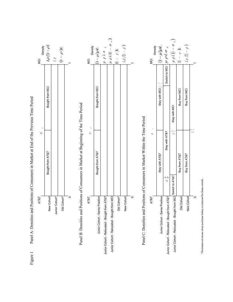
AT&

TM

CI

New

Coh

ort

Juni

or C

ohor

t*

Old

Coh

ort* 0

1

AT&

TM

CI

Juni

or C

ohor

t - S

ame

Pos

ition

Juni

or C

ohor

t - R

eloc

ated

- B

ough

t fro

m A

T&T

Juni

or C

ohor

t - R

eloc

ated

- B

ough

t fro

m M

CI

Old

Coh

ort*

New

Coh

ort 0

1

AT&

TM

CI

Juni

or C

ohor

t - S

ame

Pos

ition

Juni

or C

ohor

t - R

eloc

ated

- B

ough

t fro

m A

T&T

Sw

itch

to M

CI

Juni

or C

ohor

t - R

eloc

ated

- B

ough

t fro

m M

CI

Sw

itch

to A

T&T

Old

Coh

ort

New

Coh

ort 0

1

*

Pur

chas

es n

ot s

how

n si

nce

purc

hase

his

tory

is ir

rele

vant

for t

hese

coh

orts

.

Bou

ght f

rom

AT&

TB

ough

t fro

m M

CI

Bou

ght f

rom

MC

I

Figu

re 1

Pan

el A

: Den

sitie

s and

Pos

ition

s of C

onsu

mer

s in

Mar

ket a

t End

of t

he P

revi

ous T

ime

Perio

d

Pan

el B

: Den

sitie

s and

Pos

ition

s of C

onsu

mer

s in

Mar

ket a

t Beg

inni

ng o

f the

Tim

e Pe

riod

Den

sity

Den

sity

Bou

ght f

rom

AT&

T

Buy

from

AT&

TB

uy fr

om M

CI

Pan

el C

: Den

sitie

s and

Pos

ition

s of C

onsu

mer

s in

Mar

ket W

ithin

the

Tim

e Pe

riod

Sta

y w

ith A

T&T

Sta

y w

ith M

CI

Buy

from

AT&

TB

uy fr

om M

CI

Sta

y w

ith A

T&T

Sta

y w

ith M

CI

Den

sity

Aσ

()

Lρ

μ−

1

AL

σρ

μ

()

AL

σρ

μ−

1

()L

ρ−

1

()

ρρ

−1

L

Aσ

Aσ

Nt Az

R Az

R Mz

O Az

()

Lρμ

−1

ALσ

ρμ

()

AL

σρ

μ−

1(

)Lρ

−1

()

ρρ

−1

L

()

ρρ

−1

L

ρL (

)Lρ

−1

Figure 2: Equilibrium Prices as a Function of Switching Costs from Theoretical Model for Selected Parameter Values

Prices for σ=0.1, δc = 0.1, δf = 0.3, ρ = 0.1

0.94

0.96

0.98

1

1.02

1.04

1.06

1.08

0.1 0.2 0.3 0.4 0.5 0.6 0.7 0.8 0.9

Switching Costs

Pric

e

Prices for σ=0.5, δc = 0.1, δf = 0.3, ρ = 0.9

0.94

0.96

0.98

1

1.02

1.04

1.06

1.08

1.1

0.1 0.2 0.3 0.4 0.5 0.6 0.7 0.8 0.9

Switching Costs

Pric

e

Prices for σ=0.9, δc = 0.5, δf = 0.1, ρ = 0.5

0.94

1.04

1.14

1.24

1.34

1.44

1.54

1.64

0.3 0.4 0.5 0.6 0.7 0.8 0.9

Switching Costs

Pric

e

mu=0.1 mu=0.2 mu=0.3 mu=0.4 mu=0.5 mu=0.6 mu=0.7 mu=0.8 mu=0.9

Figure 3 Distribution of Origination and Revision Dates for VPN Contracts in Sample

umber of AT&T VPN contracts originated and revised in each quarter during the sample period. Sample

0

5

10

15

20

25

30

35

40

2Q 90 3Q 90 4Q 90 1Q 91 2Q 91 3Q 91 4Q 91 1Q 92 2Q 92 3Q 92 4Q 92 1Q 93 2Q 93 3Q 93 4Q 93 1Q 94 2Q 94 3Q 94 4Q 94 1Q 95

Freq

uenc

y

Revised Original

Nincludes the 219 AT&T VPN contracts issued between February 1990 and October 1994.

Figure 4 Margins on AT&T and MCI Stand-Alone Toll-Free and Toll Services Between Fourth Quarter of 1988 and First Quarter of 1999

0.0600

0.0800

0.1000

0.1200

0.1400

0.1600

88/4 89/2 89/4 90/2 90/4 91/2 91/4 92/2 92/4 93/2 93/4 94/2 94/4 95/2 95/4 96/2 96/4 97/2 97/4 98/2 98/4 Year/Quarter

0.0000 0.1000 0.2000 0.3000 0.4000 0.5000 0.6000 0.7000 0.8000 0.9000 1.0000

AT&T Toll-FreeMCI Toll-FreeAT&T TollMCI TollAT&T ShareMCI Share

Portability

Shar

e

Mar

gin

(cen

ts)

Figure 5 Distribution of Durations for Sample of AT&T VPN Contracts

ercentage of contracts in the sample of 219 AT&T VPN contracts that expire in the given number of sued

0.0%

10.0%

20.0%

30.0%

40.0%

50.0%

60.0%

70.0%

3 4 5 6 >6

Duration (Years)

Pre-Portability Post-Portability

Pyears. The light shaded bars are for contracts issued before portability and the dark bars for contracts isafter portability.

Appendix 1 Position of Marginal Young Consumer

The marginal new consumer is indifferent between buying from AT&T and MCI after considering the effect it has

on her future utility:

( ) ( ) ( )( ) ( )[ ] =⎪⎭

⎪⎬

⎫

⎪⎩

⎪⎨

⎧−−−+

⎥⎥⎥

⎦

⎤

⎢⎢⎢

⎣

⎡−−−−+−−−+−− ∫∫ N

AA

z

M

z

ACNAA zPrdbbsPrdbbPrzPr

RA

RA

'1

'

0

' 111'

'

μμρδ

( ) ( ) ( ) ( )( ) ( ) ( )[ ]⎪⎭

⎪⎬

⎫

⎪⎩

⎪⎨

⎧−−−−+

⎥⎥⎥

⎦

⎤

⎢⎢⎢

⎣

⎡−−−+−−−−+−−− ∫∫ N

AM

z

M

z

ACNAM zPrdbbPrdbbsPrzPr

RM

RM

11111 '1

'

0

'

'

'

μμρδ

where is the consumers’ discount factor and primes indicate next period values. On the left-hand side of the

equation is the consumer’s discounted expected utility from purchasing from AT&T. The first term is the profit

obtained in the current period. The two integrals measure the utility if the consumer’s position changes in the next

period and are multiplied by

Cδ

μ , the probability that they change. The first integral measures expected utility if the

consumer buys from AT&T again while the second integral measures expected utility if she switches to MCI. The

last term on the left-hand side measures the expected utility if the consumers’ preferences do not change. The right-

hand side is analogous if the consumer purchases from MCI. The utilities in later periods cancel out since the

consumer will purchase from her favorite firm regardless of previous purchase history. Using

( )''' 21 AAM ePP σ−=− , , szz RM

RA =− '' ( )''''' 2111 AAM

RM

RA ePPzz σ−+=+−=+ ,

and ( ) ( ) ( ) ( )( )'''2'2' 2111 AAMRM

RA esPPszz σ−+=−+=−

( ) ( ) ( )( ) ( )[ ] ( ) OAA

RMA

RAA

NAAA zzzzf 2' 1111 ρσμσσμρρρσσ −+−+−+−+== :

( ABANA PPbaaz −++= σ21 ) where

( ) ( ) ( )( )( ) ( ) ( )( )( ) ( )( )( )( )see

seseea

C

C

−+−+−+−−+−−−−−+−+

=111112

1113212111 22

1 ρμρρδρρμρρμρρρδ

,

( ) ( )( )( ) ( )( )( )( )see

sea

C

C

−+−+−+−−−

−=11111

111 22

2 ρμρρδμρρδ

and ( ) ( )( ) ( )( )( ) ( )( )( )( )see

seb

C

C

−+−+−+−−−−−−

=111112

111111 2

ρμρρδμρμρδ

.

The coefficients for AT&T’s market share transition function, ( )AAf σ are:

( ) ( ) ( ) ( ) ( eesbea +−

++−−++= 12

112

12

1ρμ

ρρρη ) and ( ) ( ) ( )( ) ( ) eesbea 22 11112 ρμρρρθ −−−−+−+−= .

A1

Appendix 2 Solving the Theoretical Model

Substituting (2) into (3), (4), (5), (6) and (8) and then these five equations into (9), I can equate the coefficients in

(10) to those in (1) to obtain:

(A1) ( ) ( )( ) ( )21 2

11 ηηδμρρ mlkesSbeaScdk F +++⎟⎟⎠

⎞⎜⎜⎝

⎛⎟⎠⎞

⎜⎝⎛ +−

++−−=

(A2) ( ) ( )( ) ( ) ( )( ) ( )( ) ( )ηθθδμρρμμρρ mlesSbeaSeSesSbeaScdl F 22

11121 12 ++⎟⎟⎠

⎞⎜⎜⎝

⎛⎟⎠⎞

⎜⎝⎛ +−

++−+−+−+−−−=

(A3) ( )( ) ( ) ( )( ) 22 121 θδμμρρ mSesSbeaSem F+−+−+−−=

Maximizing (10), the first-order condition is:

(A4) ( ) ( ) ( ) ( ) +⎥⎥⎦

⎤

⎢⎢⎣

⎡−+⎟

⎟⎠

⎞⎜⎜⎝

⎛−++−−

A

OA

A

RM

AA

RA

AA

NA

A Pz

Pz

Pz

Pz

cP∂∂

ρ∂∂

σ∂∂

σμρ∂∂

ρρ 111

( ) ( )( ) ( ) ( )[ ] ( ) 021111 =++−+−+−++−A

AAF

OAA

RMA

RAA

NA P

fmflzzzz

∂∂

δρσμσσμρρρ

The second-order condition for the problem is:

(A5) ( ) ( ) ( ) 0211122

<⎟⎟⎠

⎞⎜⎜⎝

⎛+

⎥⎥⎦

⎤

⎢⎢⎣

⎡−+⎟

⎟⎠

⎞⎜⎜⎝

⎛−++−

A

AF

A

OA

A

RM

AA

RA

AA

NA

Pf

mPz

Pz

Pz

Pz

∂∂

δ∂∂

ρ∂∂

σ∂∂

σμρ∂∂

ρρ

I confirm in my numerical solutions that this holds. Substituting the equilibrium market shares (3) for , (4) for

, (5) for and (6) for into the first-order condition and using (2) yields:

NAz

RAz R

Mz OAz

(A6) ( ) ( ) ( ) ( ) ( )( )⎢⎣

⎡+⎟

⎠⎞

⎜⎝⎛ −

+−++−++−+⎥⎦

⎤⎢⎣⎡ −+−−−− AAAAA eessbeaabcP σσμρσσρρρμρρρ

212111

211 21

( ) ( ) ( )( )( ) ( )( ) ( )( ) 0112122111

211 =⎟

⎠⎞

⎜⎝⎛ −+−+++−⎥⎦

⎤−+−+− ρμρρρθσηδσρσμ bmle AFAA

A2

Solving for and equating the constants to those in (2) yields: AP

(A7) ( )( ) ( ) ( )( )

( ) ( )ρμρρρ

ρμρρρηδμρρρ

−++−

⎟⎠⎞

⎜⎝⎛ −+−++−⎟

⎠⎞

⎜⎝⎛ +−

++−+=

1211

11212

211 1

b

bmlesbeacd

F

(A8) ( )( ) ( ) ( ) ( )( )

( ) ( )ρμρρρ

ρμρρρθδμμρρρ

−++−

⎟⎠⎞

⎜⎝⎛ −+−+−−+−+−−

=1

211

11212121 2

b

bmesbeae

F

I use Mathematica to solve equations (A1) through (A3), (A7) and (A8) analytically. I first solve equations (A8) and

(A3) to eliminate and obtain e as a function of m θ . This is a quadratic equation in which yields up to two

roots as a function of . I then use this result along with (8) to eliminate e and solve for

e2θ θ as a function of the

other parameters. This yields a quartic equation in θ which can yield up to four roots for each of the two possible

values for . This can produce up to eight possible values for e θ . I choose the stable solution(s) (i.e. 1≤θ )1. In

all my solutions, I obtained a unique stable solution.

All of the coefficients can then be calculated. Equation (3) yields , and , (8) yields 1a 2a b η , (A3) yields , (A2)

yields l , (A7) yields and (A1) yields k . Finally, I check that the necessary constraints on the problem are

satisfied (the second order condition is met, individual rationality for each of the marginal consumer types holds and

the marginal young consumer prefers to purchase when young rather than waiting to purchase until old).

m

d

In all my numerical solutions, θ and e have been positive. This implies that if firms’ shares are not equally

divided, the firm with the larger share prices higher than the firm with the small share and that firms’ shares

converge to one-half over time. Also, in all my numerical solutions, and have all been positive so that the

firms’ profits are increasing in its share.

lk , m

1 Note that if θ > 1 the firms’ shares diverge. A3

Appendix 3 Data Sources & Methods

5,..,2,1, =jw ji (Mix of voice usage): Contracts specify four types of ports corresponding to telephone numbers.

Measured ports and rate option 1 measured remote ports were toll numbers carried over a dedicated line. Rate

option 2 measured remote ports were toll-free numbers carried over a dedicated line. Outside ports were toll

numbers carried over switched lines. Separate documents, not publicly available, specified port access telephone

numbers that defined the total number of toll-free numbers carried over switched or dedicated lines. The following

matrix defines the five types of voice services that contracts can contain:

Calls To

Measured port or Rate option 1

measured remote port

Rate option 2 measured remote

port Outside ports Measured port or rate option 1

measured remote port 1 2

Outside ports 2 3

Cal

ls F

rom

Port access telephone numbers 4 5

Let equal the number of measured ports, rate option 1 measured remote ports, rate option 2 measured

remote ports, outside ports and port access telephone numbers in contract i . Based on the above matrix, the

weights assigned to voice service in contract , , is given by the equations:

im ir1 ir2

io ip

j i jiw ,

( ) iiiii rmwww 12 4,1,1, +=++ ii rw 25, =

( ) iii oww =+ 3,2,2 iii pww =+ 5,4,

Because the contract provides and but not and (since they do not affect AT&T’s fixed costs),

we have four equations and seven unknowns. Using the assumptions in MacAvoy (1995, p.107), I assume

and . Finally, I impose:

ii rm 1, ir2 io ip

1,2, 25.3 ii ww = 1,3, 75.0 ii ww = { }2,5,4, ,75.025.3max iii www = (off-to-on toll-free calls

occur in at least as high a proportion to off-to-off toll-free calls as off-to-on toll calls do to off-to-off toll calls, and

there are at least as many off-to-on toll-free calls as off-to-on toll calls). I solve these seven equations and impose

to express the weights as fractions. 15

1, =∑

=jjiw

A4

5,...2,1,, =jp tjiA (per-minute voice prices): Contracts tailor per-minute voice rates to time of day and distance. I

use the per-minute rate for the most common call placed, a daytime call of four hundred miles. Contracts often

contain monthly volume discounts for voice service. In applying these discounts I assumed the user consumed

and mix of voice usage given by . irevenue jiw ,

5,...,2,1=jctj (Marginal cost of voice usage): Marginal cost of voice calls includes access fees, operational costs

and, for toll-free calls, database lookup fees. IXCs pay LECs per-minute access fees, which are regulated and

published in tariffs with the FCC, to complete the switched portion of calls. Access fees vary across the five call

types depending on whether neither, one or both ends of the call are switched. Since access fees vary slightly across

LECS and the telecommunications operations of VPN users span multiple LECs, I use an average across all LECs

published in FCC (1999). Access fees declined during the period of my study as the FCC shifted the cost of the

local infrastructure toward monthly fees for residential long-distance consumers. I take estimates of operational

costs from court testimony by AT&T in their June 1990 application to provide intrastate toll-free service in

California.2 Operational costs are constant over all output levels until demand exceeds the capacity of the lines.

There is significant evidence that the three firms’ capacity constraints were not binding during the time period of my

study. Huber et. al. (1992, p.321) cites several studies. Another possible capacity constraint is the supply of toll-free

numbers, but the industry did not run out of numbers for the 800 prefix until 1996, and 60% of the numbers were

still available in April 1993 (FCC, 1999). After portability, the FCC allowed the LECs to charge a per-query fee to

the IXCs for each lookup of an 800-number. Since this fee varied across LECs and VPN users generally span

multiple LECs, I average across the nine major LECs and assume the average length of a toll-free call is 3.6

minutes.3

irevenue (Monthly contract revenue): 120% of the minimum volume commitment per month specified in the

contract. Users avoid falling below the minimum because penalties require paying the shortfall, and exceeding the

minimum by too far since they could have negotiated further volume discounts under a larger contract.

A5

2 John Sumpter estimated operational costs for switched toll service to be 1.01 cents, switched toll-free service to be 1.08 cents, dedicated toll service to be 1.30 cents and dedicated toll-free service to be 1.29 cents in testimony on behalf of AT&T to obtain authority to provide intrastate service in California. Application of AT&T Communications of California, Inc. (U 5002 C), June 18, 1990 as reported in MacAvoy (1996). 3 The nine LECs for which I have data are Ameritech, Bell Atlantic Corp., BellSouth Corp., Nynex, Pacific Telesis Group, Southwestern Bell Corp., US West Inc., GTE Telephone Co. and Southern New England Telephone Co. This data is taken from “Rates May Deter Use of 800 Portability,” Network World, May 10, 1993, pp. 23, 24 and 34. 3.6 minutes is average length of call according to Strategic Telemedia (1996), p. 64.

Telecommunications consultants generally advise users to sign contracts so that expected usage is 120% of revenue

commitment.

iduration (Contract duration): The minimum time commitment allowed under the contract. The exit penalties on all

contracts required users to pay the minimum revenue commitment in each year of the contract regardless of how

many minutes they consumed. Since prices were falling during this period, the minimum time commitment was

most favorable to users.

idurationtA−σ (AT&T’s previous market share of toll-free services): Annual toll-free revenue estimates by firm are

available from Levinson, et. al. (1990) from 1985 to 1990 and Strategic Telemedia (1997) from 1992 to 1997. To

concatenate these two sources, I stacked them in a regression on an AT&T dummy, an MCI dummy, a source

(Levinson versus Strategic Telemedia) dummy and an estimate of total long-distance revenues from the FCC

(1998). Using the regression results, I obtained predicted values of annual toll-free revenues assuming that Strategic

Telemedia was the source. To obtain quarterly revenues, I assumed the same seasonality as total long-distance

revenues reported in FCC (1998). Since I do not have estimates of toll-free revenues by user size, I assume that the

time trend in quantities is the same for different sized users.4

ivdisp (Voice network dispersion): Number of remote dedicated voice lines as a fraction of total number of

dedicated voice lines. IXCs leased dedicated voice lines from the LECs paying per-month fees regulated and

published in tariffs filed with the FCC. Dedicated voice lines are of two types: access (high-volume lines

terminating at an AT&T switching office) or remote (low-volume lines terminating at the subscriber’s premises).

The number of access lines is equal to the number of measured ports ( )im specified in the contract. The number of

remote lines is equal to the number of rate option 1 and 2 remote ports ( )irr 211 + .

4 The Telecommunications Market Sourcebook (Frost & Sullivan, 1995) provides evidence that the mix in revenues did not change much between dedicated service, used primarily by large users, and switched service, used primarily by small users, between 1992 and 1998 (page 15-8).

A6