Do Short-Sellers Profit From Mutual Funds?

Evidence from Daily Trades

Salman Arif, Azi Ben-Rephael†, and Charles M.C. Lee

§

First Draft: September 15, 2014

Current Draft: May 21, 2015

Abstract

Daily mutual fund (MF) flows are highly persistent and price-destabilizing, and short-sellers

(SSs) trade strongly in the opposite direction to these flows. This negative relation is associated

with the expected component of MF flows (based on prior days’ trading), as well as the

unexpected component (based on same-day flows). The ability of SS trades to predict stock

returns is up to 3 times greater when MF flows are in the opposite direction. The resulting

wealth transfer from MFs to SSs is most pronounced for high-MF-held, low-liquidity firms, and

is much larger during periods of high retail sentiment.

________________________________________ *

We thank Yakov Amihud, Cliff Asness, Ekkehart Boehmer, Andrea Frazzini, Clifton Green, David

Hirshleifer, Peter Kyle, Toby Moskowitz, Lasse Pedersen, Todd Pulvino, Adam Reed, Siew Hong Teoh,

Xiaoyan Zhang, Lu Zheng, and seminar participants at Indiana University, MIT, UC Irvine, the

Conference on Financial Economics and Accounting (CFEA), the NBER Market Microstructure Meeting,

the University of Minnesota Empirical Conference, the Korean Securities Association Annual

Conference, the AQR Insight Award Conference, and the State of Indiana Finance Conference for helpful

suggestions and comments. †

Salman Arif and Azi Ben-Rephael are at the Kelley School of Business, Indiana University.

Salman Arif: arifs@indiana.edu, +1 (812) 856 – 1592. Azi Ben-Rephael: abenreph@indiana.edu,

+1 (812) 856-4068. §

Charles M.C. Lee is at Stanford GSB. clee8@stanford.edu, +1 (650) 721 – 1295.

1

1 Introduction

Traditional rational expectation models with costly information feature agents who expend

resources to become informed. These informed agents earn a return on their information

acquisition efforts by trading against the uninformed, and as they do so, the information they

possess is incorporated into prices.1 Although such models offer broad insights into the

informational role of prices, they are of less help in understanding the nature of the information

possessed by the informed. A particular limitation is that informed traders in these models are

typically identical (i.e., possess the same information and face the same cost constraints).

In real-world markets, price discovery is a much more complex process. A more realistic

characterization of the world of professional investment management is one in which multiple

groups of “heterogeneously informed” traders facing different cost constraints are seeking to

earn a competitive return on their particular parcels of knowledge.2 In such markets, efforts to

understand price discovery calls for insights into the roles played by different groups, and the

motives that each has for trading. A challenge to empiricists is to identify settings in which the

actions of distinct investor groups can be identified and studied in isolation.

In this study, we use trade data at the daily level to examine the interaction between two

important, yet largely orthogonal, investor groups – mutual funds (MFs) and short-sellers (SSs).

Both groups are prominent in the U.S. equity market. MFs are professionally managed

investment vehicles that charge an active management fee and cater primarily to a retail

clientele. With close to $6 trillion in assets under management as of year-end 2012, they

constitute a major source of active trading in the market.3 Short-sellers are another important

group of active investors, which prior studies consistently associate with superior information

processing capabilities.4

1 In equilibrium, the supply of traders with costly-to-collect information adjusts to provide just sufficient reward for

information collection and processing. Thus the cost constraints faced by informed traders are reflected in the level

of informational efficiency attained by the market. See for example, Admati (1985), Diamond and Verrecchia

(1981), and Verrecchia (1982). 2 Stefanini (2006) surveys investment strategies used by hedge funds. Difference-of-opinion models (e.g., Varian

(1989), Harris and Raviv (1993), and Kandel and Pearson (1995)) may be viewed as an attempt to address this facet

of reality. See Hong and Stein (2007) for a review of this literature. 3 See the 2013 Investment Company Factbook, available at http://www.icifactbook.org

4 Boehmer, Jones and Zhang (2008) report short-selling accounts for over 20% of the trading volume in the U.S.

We discuss other related short-selling studies in Section 2.

2

Although MF managers tend to be regarded as sophisticated investors, they are also subject

to a variety of regulatory and agency-related constraints that may impede fund performance.

Prior evidence suggests that at least some subset of MF managers possess persistent stock-

selection skill, although as a group MFs seem to curiously underperform.5 Indeed, a number of

recent studies (summarized in Section 2) show that MF trading can lead to predictable return

patterns at the individual stock level. However, prior studies that examine institutional investor

behavior typically rely on quarterly holdings culled from 13-F filings, which offer limited

insights on daily trading activities (e.g., Kacperczyk, Sialm, and Zheng (2008) and Puckett and

Yan (2011)). In addition, because these filings only reflect the long-side of investors’ positions,

no distinction can be made between the actions of MFs and SSs.

Using highly granular trading data, we provide the first close-up evidence on how these two

investor groups interact with each other at the daily level, as well as the implications of their

interaction for future stock returns. The two-folded focus of our investigation is on: (1) the

responsiveness of daily SS trades to the direction of MF flows (i.e., whether SSs seem to detect

and trade on patterns in MF flows), and (2) the implications of daily MF and SS interactions for

future stock returns (i.e., the extent to which their interactions result in a wealth transfer from

MFs to SSs).

Prior studies provide virtually no guidance on how these two groups of investors might

interact at the daily level. Ex ante, a case might be made for either a positive or a negative

correlation, or no correlation at all. For example, if MFs and SSs generally respond to similar

information, the two groups may on average trade in the same direction. Conversely, short

sellers may have superior information sets or higher processing speed relative to mutual funds.

Moreover, if mutual fund trading pressure results in temporary price dislocations that are

anticipatable by SSs, SSs may systematically exploit these patterns. In these latter scenarios,

short-sale activities would be, on average, in the opposite direction to trades by mutual funds.

5 Kacperczk et al. (2008) and Puckett and Yan (2011) show that the interim trades by MF managers are performance

enhancing, even after costs, and that top MFs by this measure outperform consistently. Other studies show, taken as

a whole, MFs tend to underperform (e.g., Gruber (1996), French (2008), Fama and French (2010)). Relatedly,

Bennett, Sias and Starks (2003), Cai and Zheng (2004), and Yan and Zhang (2009) find institutional trades, inferred

from changes in quarterly 13-F holdings, do not predict future returns. More recently, Del Guercio and Reuter

(2014) show MFs that are directly-sold to investors do not underperform – i.e., the MF underperformance is driven

primarily by funds sold through affiliated brokers.

3

To track the daily trades of mutual funds, we use information from a database provided by

Ancerno Limited. Ancerno is a widely-recognized transaction-cost consulting firm to

institutional investors, and our database contains all trades made by Ancerno’s substantial base

of clients. During our study period (January 2005 to July 2007), Ancerno’s MF clients alone

accounted for 13.65% of the average daily trading volume in our sample stocks.6 We use this

data to compute a measure of the daily directional flow across all MFs.7 Specifically, for each

stock, we compute “MFt”, defined as the number of shares purchased by MFs minus the number

of shares sold by MFs on day t, divided by that day’s total share volume traded.

We then compare the daily directional MF flow to the volume of newly-initiated short sales,

computed using data from the NYSE Trade and Quote (TAQ) regulation SHO database.8 The

regulation SHO database contains tick-by-tick short-sale data for a cross-section of more than

3,800 individual stocks. We aggregate the short sales information for each stock to the daily

level. In particular, we focus on “SSt”, a measure of the total number of shares traded in short-

seller initiated transactions, expressed as a percentage of total daily share volume. During our

sample period, a vast majority of mutual funds either do not take or are prohibited from taking

short positions. We can therefore confidently exclude MF-initiated trades from those initiated by

SSs in the SHO database.9 Our research design thus provides a unique opportunity to compare

and contrast the directional trading activities of two purportedly sophisticated sets of investors

whose actions are mutually exclusive.

Our first main result is that daily SS and MF trades are highly interdependent. At the daily

level, SSs trade strongly in the opposite direction to MFs. On days when MFs are net buyers

6 Our sample period is limited to regulation SHO short-selling database availability (see Footnote 7). We discuss the

Ancerno dataset in more detail in Section 2. Other studies that have used this database include: Chemmanur, He,

and Hu (2009), Goldstein, Irvine, and Puckett (2011), Puckett and Yan (2011, 2013), Anand, Irvine, Puckett and

Venkataraman (2012, 2013), Jame (2012), Busse, Green, and Jegadeesh (2012), Franzoni and Plazzi (2013), and

Gantchev and Jotikasthira (2013). None of these studies examine the MF and SS interaction. 7 We note that Ancerno provides trade level data on mutual fund trades and that the actual intraday execution times

are not available. 8 On June 23, 2004, the SEC adopted Regulation SHO to establish uniform locate-and-delivery requirements and

establish a procedure to temporarily suspend the price tests for a set of pilot securities. At the same time, the SEC

mandated that all self-regulatory organizations make tick data on short sales publicly available. This resulted in a

short-sale Pilot period during which all short-initiated trades must be self-identified. Our study covers essentially

the entire period of the regulated disclosure (the 626 trading days from January 3, 2005 to July 6, 2007, inclusively).

See Diether, Lee, and Werner (2009) for additional details on this data. 9 According to Chen, Desai, and Krishnamurthy (2013) the proportion of mutual funds that actually take any short

position in a given year has increased recently, from 2% in 1994 to 7% in 2009. So during our sample period, only

an extremely small minority of mutual funds engaged in any short selling.

4

(sellers) of a stock, we generally observe increased (decreased) SS activities. On days with

extreme MF flows (i.e. those firm-days ranked in the top-quintile by MF, either strong buy or

strong sell), SSs are on the opposite side of MF trades 71% of the time (see Panel 8.A). Even on

days with less extreme MF flows (i.e., when we include all firm-day observations), SSs are still

on the opposite side of MF flows 56% of the time.10

Both groups exhibit strong time-series persistence. Stocks that are strongly purchased (sold)

by MFs continue to be strongly purchased (sold) by MFs for multiple days. The same is true for

SS flows. These persistent time-series patterns can confound statistical inferences made from

daily data. To address such concerns, we estimate a three-equation vector auto-regression

(VAR) system. Specifically, we model daily SS trades, MF trades, and returns (RET) as

dependent variables while controlling for lagged observations of each. The resulting cumulative

impulse response functions show that a positive one standard deviation shock to MF increases

SSs by 5% of daily volume, or roughly 30% of the average daily SS. Most of this response

occurs in the next ten trading days. The MF reaction to SS is much more muted. Additional

analyses show that it is possible to conclude daily MF trading “Granger cause” SS activities, but

not vice versa.

To shed light on how SSs are able to detect and respond to MF flows, we parse each day’s

MF trading into two components – ExpMF (the expected amount of MF flow based on

information available at the beginning of each day), and UnexpMF (the unexpected MF flow,

based on same-day trades). If SSs are responding primarily to longer-term expected MF flows

that are predictable in advance, we would expect a significantly negative coefficient on ExpMF.

Conversely, if SSs are reacting primarily to same-day MF trades, the loading on UnexpMF

should dominate.

Our results show that SSs are responsive to both ExpMF and UnexpMF. On average, a one

standard deviation increase in ExpMF (UnexpMF) is associated with an 8.25% (6.0%) increase

in the daily short-initiated volume. The larger effect associated with ExpMF suggests that daily

SS trading is more sensitive to MF flows that were anticipatable by the beginning of trading each

10

The SS variable is demeaned at the firm-level so we can make daily directional inferences. Note that although

MFs and SSs disagree more often than they agree, their directional trades are far from a “zero-sum” game. Our

results show are other sizable players in the market (e.g., retail investors, other institutions, or “short covers”), and

on days when MF and SS are in directionally concordant, someone else is providing liquidity to both groups.

5

day. However, the economic and statistical significance of UnexpMF show that same-day MF

buys also somehow are being telegraphed to SSs, who respond by increasing their short-sell

volume.

We next investigate the implications of MFs and SSs flows for future stock returns. We find

that directional MF flows are generally price destabilizing. Stocks experiencing strong MF buys

(sells) on a given day have typically already been bought (sold) by MFs for the past 15 trading

days. Moreover, extreme MF buys (sells) portend future negative (positive) abnormal returns

over the next 63 days. Closer analyses show the “daily shock” to MF (UnexpMF) initially leads

to short-term price continuation, lasting up to three days. However, over longer horizons, prices

revert. These findings are consistent with MF herding leading to price destabilization in the

short-run (Puckett and Yan (2013)). Indeed our evidence augments prior findings by showing

that the MF herding phenomenon is pervasive, and has long-lasting implications for future

returns.

Interacting SS with MF, we find that SSs benefit from the price reversals associated with MF

trading – i.e., SSs earn higher profits when they trade against MFs. Nagel (2012) and So and

Wang (2014) nominate the profitability of short-term price reversal strategies as a measure of the

compensation earned by liquidity providers. Interpreted in this light, our findings are consistent

with SSs serving as strategic liquidity providers to MFs, and earning a positive return from this

activity over time. A large literature (see Section 2) suggests SSs possess superior ability to

process fundamental information. Our findings show that the SSs’ informational advantage is

also related to their role as strategic liquidity providers to MFs.

Using weekly-aggregations, we confirm that MF-induced price reversals are a longer horizon

phenomenon. A cash-neutral strategy based solely on betting against net MF flows yields an

abnormal month return of 1.37% over a 63-day holding period.11

Given the economic

significance of these price reversals, we further examine whether SSs profit by betting against

MF trades. Strikingly, we show that returns to the well-documented SS trading strategy (e.g.

Boehmer et al 2008; Diether et al 2009) are up to three times larger when SSs trade against MFs

(i.e., when they “disagree”) than when SSs trade in the same direction as MFs (i.e., when they

11

Consistent with prior literature, we also document that a long-short strategy based solely on SS yields an abnormal

return of 1.60% over a 63-day holding period.

6

“agree”).12

Specifically, over a 63-day holding period, returns to a SS strategy where MFs and

SSs disagree earns 1.98%, while a SS strategy where MFs agree earns only 0.57%. This gap is

consistent with SSs profiting from MF-induced price reversals. Taken together, these findings

strongly suggest that SSs are able to detect and capitalize on MF trading activity.13

Finally, we examine several situations in which MFs might experience the greatest difficulty.

First, consistent with a price-pressure explanation, we find that the wealth transfer from MFs to

SSs is most pronounced in stocks with larger MF institutional ownership and lower overall

liquidity. In addition, consistent with a behavioral-based explanation, we find this wealth

transfer effect is much higher during periods of high retail investor sentiment.14

During high

sentiment periods, the volume of daily MF trading at the firm-level increases on average by 8.8%

for large (top quintile) firms and 28% for small (bottom quintile) firms. At the same time, the

implied wealth transfer from MFs to SSs increases dramatically relative to low sentiment periods

(total losses to SSs average 2.10% higher per firm over the next 63-days). Further analyses

show that this effect is directly linked to the increase in MF trading volume, and is not due to an

increase in net MF buying during high sentiment periods.

Collectively, our findings provide at least a partial explanation for the MF performance

puzzle. A curious finding from past studies is that active MFs consistently underperform their

passive benchmark. We show that at least some of this underperformance is potentially

attributable to a net wealth transfer between MFs and SSs, which is most pronounced when MFs

trade stocks with high institutional ownership and low liquidity. Our results also provide a direct

link between MF losses and retail investor sentiment. Consistent with the behavioral literature,

MFs lose more to SSs when retail investors are overoptimistic about equities.

12

The ‘Disagree’ portfolio consists of a long position in the portfolio of stocks with low short selling and high

mutual fund selling and a short position in the portfolio of stocks with heavy short selling and heavy mutual fund

buying. Thus, these portfolios consist of stocks where short sellers and mutual funds trade in opposite directions.

Conversely, the ‘Agree’ portfolio consists of a long position in stocks with heavy mutual fund buying and light short

selling, and a short position in stocks with heavy mutual fund selling and heavy short selling. In this case short

sellers and mutual funds trade in the same direction. 13

Two caveats are in order. First, because mutual fund trading data are not typically available in real time, this is

not a tradable strategy. Second, we do not have data on when short-sellers close their positions, so we only estimate

their profits based on hypothetical holding periods. Prior studies that estimate short-sale holding periods (e.g.,

Boehmer, Jones, and Zhang (2008)) report a median duration of 37 trading days, which is ample time for the short-

sellers in our study to profit from trading in the opposite direction to MFs. 14

We use the Ben-Rephael, Kandel and Wohl (2012) measure of retail investor sentiment, which captures the

monthly flow of retail money from bond funds to equity funds within the same mutual fund family.

7

Our findings also shed new light on the predictive power of SS trades for future returns. We

show that much of the SSs predictive power is due to their tendency to trade in the opposite

direction to MFs. In addition, we find SSs respond both to expected MF flows (based on prior

trading), and to unexpected shocks in MF trades on the same day. The former can be linked to

the earlier literature on capital flow-induced MF trading.15

The latter is a higher-frequency

phenomenon associated with mutual fund herding. Despite efforts to engage in stealth trading

and manage their costs through more skillful trading desks (e.g. Alexander and Peterson (2007),

Anand et al. (2012)), evidently MFs are still telegraphing their trades to some SSs.

On a related note, our findings may also help to explain the main finding in Stambaugh, Yu

and Yuan (2012; SYY). SYY report that the short-leg of multiple market pricing anomalies is

only profitable during high sentiment periods. We find that it is precisely during these periods

that the heightened trading activity of MFs becomes most vulnerable to SS activities. Thus it

appears that the short-leg profitability documented by SYY may come in part at the expense of

retail (MF) investors, who lose to SSs during such times.

Finally, our findings are related to the literature on predatory trading. Brunnermeier and

Pedersen (2005) present a model in which some traders induce and/or exploit the need of other

traders. In the same spirit, Chen, Hanson, Hong and Stein (2008) show that, in time series, the

average return of 45 hedge funds are significantly higher in months when a larger fraction of

MFs are in distress. Using monthly open short interest data, they find evidence that the short-

sale ratio increases in advance of sales by distressed MFs. Our results are consistent with these

findings, but we provide a much clearer view of the direct link between MF trades and SS

activities.

The rest of the paper is organized as follows. Section 2 discusses related literature on why

MF flows might be predictable. Section 3 describes the data and provides summary statistics.

Section 4 presents our empirical results on the relationship between MF and SS trades. Section 5

reports the implications of these trading activities for future stock returns. Section 6 explores

15

See, for example, Coval and Stafford (2007), Frazzini and Lamont (2008), Lou (2012), Shive and Yun (2013), and

Khan, Kogan, and Serafeim (2012). According to this explanation, the combination of “dumb money” flows from

retail investors and the “no leverage” restriction on MF funds conspire to generate predictable patterns in returns for

individual stocks held by these funds . The no leverage constraint is important because it prevents MF managers

from absorbing investor inflows and outflows by changing their leverage ratio.

8

short-term liquidity provision. Section 7 provides additional evidence on the return implications

of the interaction between MFs and SSs in the cross-section and time-series. Section 8 concludes

with a summary of the key results and a discussion of their implications for future research.

2 Related Literature

Prior studies suggest at least two reasons why the direction of daily MF trades might be

predictable. First, MF trades are a function of investor flows in the retail market and are thus

vulnerable to fluctuating investor sentiment. When market-wide sentiment is bullish (bearish),

equity MFs experience inflows (outflows). These flows generate non-fundamental price pressure

on aggregate stock prices that revert in the future.16

At the same time, in the cross-section of

mutual funds, poorly performing managers are vulnerable to redemption pressures, while high

performing managers need to quickly equitize their new inflows. Thus the stocks held by MFs

are prone to predictable directional flows that result in price pressure in the short-run, and return

reversal in later periods. Prior studies show such flow-induced return patterns can be both

statistically and economically significant (e.g., Frazzini and Lamont (2008), Coval and Stafford

(2007), Lou (2012)). Indeed, the evidence in Coval and Stafford (2007), Lou (2012), Dyakov

and Verbeek (2013) and Shive and Yun (2013) strongly suggest these predictable patterns are at

least somewhat exploitable based on MF holdings as reported in quarterly 13-F filings.

Second, if the directional trading of individual MFs is correlated at the stock level (a

phenomenon sometimes referred to as MF “herding”),17

their collective actions can generate

substantial short-term price pressure. Even if the past performance of a particular fund does not

offer clear guidance as to the direction of future flows in a stock (e.g., if the particular MF in

question is a mediocre performer in past months), the act of trading itself can still exert price

pressure. If the buy-sell direction of MF trades in a given stock are positively correlated across

funds (for example, due to common retail sentiment, or similarities in their investment

strategies), these flows will again lead to short-term price pressure, which translates into higher

trading costs for MFs, and subsequent return reversals for the stocks they trade.

16

For example, see Baker and Wurgler (2000), Dichev (2007), Ben-Rephael et al. (2012), and Arif and Lee (2014). 17

See, for example, Puckett and Yan (2013).

9

MFs and other institutional investors are, of course, aware of the price pressure

problem. Prior studies on stealth trading show larger institutions (including MFs) attempt to hide

their trades and reduce price impact by using mid-sized trades and by clustering in round

amounts, such as 500, 1000, and 5000 shares (Alexander and Peterson (2007) and Chakravarty

(2001)). Other institutions engage trading-desks and trade-cost consultants to help mitigate the

problem (Anand, Irvine, Puckett, and Venkataraman (2012)). Nevertheless, given their size and

the likelihood that their trades are directionally correlated over time, we expect MFs, as a group,

to remain vulnerable to the price pressure problem.

At the same time, prior studies consistently find that short-sellers are highly sophisticated

investors (e.g., Boehmer, Jones and Zhang (2013), Drake et al (2011), Engelberg, Reed, and

Ringgenberg (2012), and Dechow et al. (2001)). At the intraday level, short-sale flows improve

the informational efficiency of intraday prices (Boehmer and Wu (2013)). Globally, the

introduction of short-selling in international markets is associated with a lowering of country-

level costs-of-capital, an increase in market liquidity, and an improvement in overall pricing

efficiency (Daouk et al. (2006), Bris et al. (2007)). In the cross-section, increased short selling

activity has been associated with lower subsequent stock returns (Beneish et al. (2013), Diether

et al (2009), Boehmer et al (2008)), and elevated levels of short selling has been observed prior

to disappointing earnings announcements (Cristophe et al (2004)), analyst downgrades

(Cristophe et al (2010)), disclosures of financial misconduct (Karpoff and Lou (2010)), and

insider sales (Khan and Lu (2013)).

In this study, we are particularly interested in how short selling activities are affected by MF

flows. Prior studies provide virtually no guidance on how the daily directional trades of these

two groups might be related. Ex ante, a case might be made for either a positive or a negative

correlation, or no correlation at all. For example, mutual funds and short sellers may on average

trade in the same direction if they respond to similar information sets. Conversely, short sellers

may have superior information sets or higher processing speed relative to mutual funds.

Moreover, if mutual fund trading pressure results in temporary price dislocations, SSs may

systematically exploit these patterns. In these latter scenarios, short-sale activities would be, on

average, in the opposite direction to the trades by mutual funds. We explore each of these

possibilities.

10

In sum, prior research suggests that the direction of daily MF trades may be predictable

because of either: (1) lower frequency flow-induced trading associated with retail investor fund

inflows and outflows, or (2) higher frequency problems associated with “crowded trades” at the

daily level. We provide evidence on the relative importance of these two types of MF flows in

explaining the level of daily SS activities. We also evaluate the extent to which these patterns in

MF trading contribute to a wealth transfer from MFs to SSs.

3. Data and Summary Statistics

3.1 Data

3.1.1 Regulation SHO Short Sale Database

We obtain short sale data from the NYSE Trade and Quote (TAQ) Regulation SHO database.

The data period ranges from January 3, 2005 to July 6, 2007 for NYSE-listed stocks and includes

all intraday trades by short-sellers. Specifically, for each short sale transaction, the data includes

the stock ticker, the number of shares traded, the execution price, and the date and time of the

transaction. The data does not include information on short covering. In addition, the data

includes an identification code for trades which are exempt from the price test rules. Usually,

these trades (with the identification code “E”) are executed by market makers (see, e.g., Evans,

Geczy, Musto, and Reed, 2009). Following Boehmer et al (2008), since we are primarily

interested in trades by informed short sellers, we exclude such trades from our analysis (they are

only a minor fraction of the sample). We match the TAQ stock tickers to CRSP using link tables

from WRDS.

3.1.2 Ancerno Institutional Trading Data

We obtain institutional trading data from Ancerno Ltd. Ancerno (formerly a unit of

Abel/Noser Corp) is a widely-recognized consulting firm that provides consulting services to

11

institutional investors to help them monitor their trading costs.18

The data is available starting

January 1999 and overlaps with our Reg-SHO 2005-2007 sample period. As mentioned in

Puckett and Yan (2011) (hereafter, “PY”), Ancerno data has several appealing features for

academic research. The data is supposed to be free of survivorship bias, self-reporting bias and

backfill bias. In addition, PY find that the characteristics of stocks held and traded by Ancerno’s

institutions are not significantly different from the characteristics of stocks held and traded by the

average 13F institution.

The Ancerno dataset provides data about trading by mutual funds and pension plans.

Using Ancerno’s client-type codes, we are able to focus on trades made by mutual funds. Our

main variables include: the date of trade (YY/MM/DD), the stock ticker and CUSIP, the number

of shares per trade, and a Buy or Sell indicator which specifies whether a trade is a buy (1) or a

sell trade (-1). A detailed explanation about Ancerno variables can be found in the Appendix of

PY. We note that the dataset provides trade level data on mutual fund trades and that the actual

intraday execution times are not available. Accordingly, for each stock, we use the Ancerno

dataset to compute the total daily mutual flow across all mutual funds. Finally, we match our

sample to CRSP using both the stock ticker and CUSIP. To ensure that the match is made

correctly, we require Ancerno’s daily close-price variable to match CRSPs close-price for any

given trade.

3.1.3 Other Variables and Final Sample

Stock prices, shares outstanding, daily volume and returns are obtained from the Center for

Research in Securities Prices (CRSP). Book values and other accounting information are

obtained from Compustat. We match the Reg SHO and Ancerno databases using CRSP’s permno

and day. We split-adjust all relevant variables using the CRSP adjustment factor. As part of our

analysis, we explore the lead-lag relation between short sales, mutual fund trades and daily

returns.

18

Previous studies that use Ancerno data include: Chemmanur, He, and Hu (2009), Goldstein, Irvine, and Puckett

(2011), Puckett and Yan (2011), Anand, Irvine, Puckett and Venkataraman (2012), Jame (2012), Busse, Green, and

Jegadeesh (2012), Franzoni and Plazzi (2013), and Gantchev and Jotikasthira (2013).

12

To compute daily abnormal returns, we apply the Daniel, Grinblatt, Titman and Wermers

(1997) characteristic-benchmark portfolio adjustment procedure (hereafter “DGTW”), which

controls for firm size, B/M, and price momentum characteristics. Specifically, we construct our

benchmark portfolios every year on June 30th

, using NYSE size breakpoints to sort stocks into

size quintiles. We then further conditionally rank on B/M and momentum, thus forming 125

benchmark portfolios. We compute daily returns for each of these 125 benchmark portfolios for

every day in our sample. These portfolios are then used to calculate daily abnormal returns for

each stock.

Finally, to reduce noise caused by microstructure issues and missing data, we apply the

following filters: (1) stocks must have a previous day price of $5 and above; (2) stocks must be

in the DGTW ranking sample. Our final sample includes 575,000 day-stock observations.

3.2 Variable Definitions and Daily Sample Statistics

The two key variables for our analyses are daily short sales for each stock (hereafter, “SS”)

and mutual funds’ daily net purchases for each stock (hereafter, “MF”), each scaled by the

stock’s total daily trading volume. Specifically, SS is the number of shares sold short multiplied

by -1, divided by total trading volume that day (expressed in %) in the stock. We multiply SS by

minus 1 to reflect the fact that a short sale is a negative net purchase (i.e., from a directional

perspective, it is a ‘sell’). MF is the aggregate net number of shares purchased by mutual funds,

divided by total trading volume that day (expressed in %). Aggregate net number of shares

purchased by mutual funds is defined as the total number of shares bought minus the total

number of shares of the stock sold by mutual funds on aggregate that day in the stock.

Table 1 Panel A presents summary statistics for our main variables. To construct this panel,

we calculate the cross sectional mean, median and standard deviation for each day, and report the

time series averages of these cross-sectional statistics. Consistent with prior work (e.g., Diether,

Lee and Werner (2009) and Engelberg, Reed and Ringgenberg (2012)), short selling represents a

substantial percentage of daily volume. On average, 18.79% of total daily trading volume is

initiated by short-sellers. Mutual fund trade volume is also high: on average, mutual funds in our

sample account for 13.65% of total daily volume (MF VOL). To provide a sense of the absolute

13

magnitude of daily MF directional trading, we also compute AbsMF, defined as the absolute

value of daily MF trading. The net directional trading by MFs is, of course, lower than their total

daily volume (MF VOL). Nevertheless, it is still quite substantial, with an average of 9.28%.

Table 1 Panel B provides some preliminary evidence on the directional concordance /

discordance of daily MF and SS trades. To construct this panel, we first demean SS at the firm-

level by subtracting the average firm-level SS. We then group each firm-day observation by the

sign of MF and the demeaned SS value independently. Table values in Panel 1.B represent the

percentage of firm-day observations in each category, where “SS Buys” refer to days when SS-

initiated volume is below firm-level mean, and “SS Sells” refer to days when SS-initated volume

is above firm-level mean.

Panel 1.B shows that, more often than not, MFs and SSs are on opposite sides of daily

trading. The off-diagonal cells show that in 56.4% (26.1% + 30.4%) of all firm-day

observations, MFs and SSs directionally disagree. However, MF and SS trades are far from a

“zero sum” game, whereby one provides liquidity for the other. Specifically, we observe that

43.6% of all firm-days (23.9% + 19.6%), MFs and SSs are directionally on the same side. On

such days, someone else (perhaps retail investors, other institutions, or “short covers”) is

supplying the liquidity.

4. Mutual Fund Flows and Short Sales

4.1 Lead-Lag Relation between Daily Mutual Fund Flows and Short Sales

We now proceed with an analysis of the lead-lag relation between the level of daily trading

by both groups. In Table 2 we report results with SS as the dependent variable. In Table 3, we

conduct similar set of tests with MF as the dependent variable. In each case, we perform day-

stock panel regressions, and include both firm and day fixed effects. Given the large number of

observations, instead of using actual firm and day dummy variables, we de-mean all the variables

of interest by firm and day. To control for additional unobservable effects, we also cluster the

standard errors by firm and day. We also control for other explanatory variables nominated by

14

prior studies such as firm-level trading volume, volatility, daily high and low prices, bid-ask

spread, stock price, and firm size (see Diether, Lee and Werner (2009) for a detailed discussion).

Table 2 explores the daily relation between SS (the dependent variable) and lagged SS,

lagged stock returns (RET) and lagged mutual fund net purchases (MF). Columns (1) and (2)

confirm the findings in Diether, Lee and Werner (2009). Specifically, Column (1) documents

strong positive persistence in short sale trading activity, with lagged short sales explaining 25%

of the variation in SS. Column (2) documents a negative relation between lagged returns and SS,

which indicates that SSs respond to short-term price changes in a contrarian fashion. Column (3)

shows that lagged mutual fund net purchases negatively predict SS. This indicates that short

sellers trade against the direction of past mutual fund flows: higher (lower) net purchases by

mutual funds are followed by heavier (lower) short selling in the future. In Columns (4) through

(7) we explore the partial effect of all variables after controlling for past returns and other firm

characteristics. We find that all variables are important determinants in explaining SS. In

particular, daily SS is negatively correlated with past MF even after controlling for past returns.

Thus, SSs are not simply contrarian traders who respond to high returns in the past. Indeed, it

appears they are also incrementally affected by MF flows. In subsection 4.2 we further explore

the economic magnitude of the MF effect on SS in a VAR framework.

Table 3 presents similar analyses with MF as the dependent variable. Column (1) of Panel A

shows directional MF flows are strongly persistent. As with SS, the Adjusted-RSQ is large

(24.61%). Column (2) explores the relation between MF and past returns. Consistent with prior

studies (e.g., Grinblatt, Titman, and Wermers (1995)) the mutual funds in our sample seem to

engage in positive feedback trading – i.e. higher past returns portend stronger MF purchases.

Column (3) shows that when the two time-series are considered in isolation, the first few lags of

SS are negatively related to MF, but that the relation turns positive as the lags increase. Given

the importance of past returns in explaining the actions of both groups, it is difficult to draw any

conclusions about SS and MF interactions without controlling for RET. Columns (5) through (7)

control for past RET as well as a host of other firm characteristics. These results show that the

overall relation between lagged SS and current MF turns reliably positive beyond the first lag.

Figure 1 provides a graphic representation of the daily trading patterns for MF and SS for

firms in the extreme MF deciles. To construct this figure, we rank all stocks in our sample each

15

day into ten deciles based on MF. We then keep the firms in the top decile (heavily bought

firms) and bottom decile (heavy sold firms). We denote the ranking day as day t, and compute

daily trading activity by mutual funds and short sellers from day t-14 to day t+63. Graphs 1.A

and 1.B plot daily and cumulative MF, respectively, for the firms in the top and bottom decile of

MF. Graphs 1.C and 1.D plot daily and cumulative SS, respectively, for the same firms (i.e.

firms in the top and bottom deciles of MF ranked on day t).

The two top graphs show the strong persistence in MFs trades. For firms that were heavily

bought by MFs, the buying began 14 days prior to day-t, and persists over the next three months.

Graph 1.B shows that the total cumulative effect (a measure of cumulative net MF buying or

selling over the entire period) is roughly 200% of average daily volume for the typical extreme

decile stock. Graph 1.C (1.D) reports the daily (cumulative) SS for the same stocks, i.e. stocks in

the extreme deciles of day-t MF. To facilitate interpretation, we plot daily SS demeaned by its

long run mean. The effect of MF flows on SS is striking: SSs appear to respond to directional

MF trades, both before and after day-t. Graph 1.D shows that in terms of long-run cumulative

economic magnitude, SS increase their activity by 20-25% of daily volume in these stocks

(relative to the average amount of daily SS for each firm).

4.2 Vector Auto Regression (VAR) Results

To assess the economic magnitude and dynamics of the relation between RET, MF and SS, we

estimate a three equation VAR (Vector Auto Regression) system of RET, MF and SS with five

lags of RET, MF and SS as follows:

5 5 5

1 1 1 1 1

1 1 1

5 5 5

2 2 2 2 2

1 1 1

5 5 5

3 3 3 3 3

1 1 1

t i t i i t i i t i t

t t t

t i t i i t i i t i t

t t t

t i t i i t i i t i t

t t t

RET RET MF SS

MF RET MF SS

SS RET MF SS

(Eq. 1)

In our main Impulse Response Function analysis (hereafter, “IRF”), we set the

contemporaneous Cholesky order to be RET, MF, and SS. This sequencing reflects our priors

16

about the order of causality among the three endogenous variables. We set RET as the first

variable because of extensive prior evidence that both MFs and SSs respond to past returns. We

set MF as the second variable because the trading decisions of mutual funds are more

constrained than short sellers. Thus it is less likely that MFs can respond quickly to daily SS

trading activity, even if this activity was detectable by MFs.19

On the other hand, it is much

more likely that SSs can respond to same-day MFs trades. As a robustness check, we also

provide the results for alternative order selection assumptions in Appendix A.20

Graph 2.A plots the accumulated response of SS to a positive one standard deviation shock in

MF (i.e., the response of SSs when MFs are net buyers). The effect of MF on SS is economically

and statistically significant. A positive one standard deviation shock to MF increases SSs by 5%

of daily volume, or roughly 33% of the average daily SS. Most of the response occurs in the

next ten trading days. Graph 2.B plots the accumulated response of MFs to a negative one

standard deviation shock in SS (i.e., the response of MFs when SSs increase their short activity).

A negative shock to SS has an initial weak positive effect on MF, but this reaction eventually

turns negative, consistent with Columns (5) and (6) of Panel B in Table 3. Thus, when SSs

increase their short selling activity, MFs also become net sellers 3-5 trading days later. Overall,

a one standard deviation negative shock to SS decreases MF by 0.8% of daily volume, with most

of this response occurring over the next ten trading days. Importantly, this relation does not seem

to be stable. Graphs A.2 and A.3 of Appendix A show that changing the response order affects

these results. Thus, we conclude that SS do not Granger cause MF.

4.3 The Contemporaneous Relation between MF and SS

Taken together, the results thus far establish a robust and economically significant lead-

lag relation between MFs and SSs. We now examine the contemporaneous relation between

daily SS, MF, and RET after taking into account the time-series patterns documented earlier.

19

MFs are restricted in their use of leverage and do not tend to short. These constraints limit their options when

confronted with daily retail investor flows (i.e. they must fully equitize inflows and redeem outflows). 20

In Appendix A we show that the order of RET in that triplet does not affect the IRF cumulative responses of MF

and SS. The order between MF and SS has an effect on the IRF magnitudes.

17

Table 4 reports results of panel regressions of SS, unexpected SS (UnexpSS), and

expected SS (ExpSS), on selected contemporaneous variables. Panel A of Table 4 shows that

daily SS is strongly negatively related to MF contemporaneously. This relation is robust across

various model specifications. In Columns (1) through (5) the dependent variable is total daily

short-selling, or SS. Column (1) shows that higher net purchases by mutual funds are associated

with heavier short selling, even after controlling for RET. Column (2) shows that the coefficient

on the interaction term (Ret*MF) is also negative, indicating that short sellers bet even more

heavily against mutual funds when same-day returns are in the same direction as MF.

Specification (3) shows that adding other stock control variables does not alter these results.

In Columns (4) and (5) we utilize our lead-lag analysis from Section 4.1 to explore the

effect of the expected and unexpected MF components on SS. Specifically, we regress MF on

five lags of SS, MF and RET and define expected mutual fund trade (ExpMF) as the fitted value

from the regression. The residual from this regression is unexpected mutual fund trade

(UnexpMF). Thus, ExpMF captures the expected amount of MF flow based on information

available at the beginning of each day, while UnexpMF captures the unexpected MF flow, based

on same-day trades. If SSs are responding primarily to longer-term expected MF flows that are

predictable in advance, we would expect a significantly negative coefficient on ExpMF.

Conversely, if SSs are reacting primarily to same-day MF trades, the loading on UnexpMF

should dominate.

Interestingly, results in Columns (4) and (5) show that the coefficients on both ExpMF and

UnexpMF are negative and highly significant, indicating that short sellers respond to both the

expected and unexpected components of mutual fund trading. On average, a one standard

deviation increase in ExpMF (UnexpMF) is associated with a 1.25% (1%) increase in daily SS,

which translates into an 8.25% (6.0%) increase in the daily short-initiated volume.21

Moreover,

adding ExpMF as an additional explanatory variable significantly improves the adjusted R-

Squared (the Adj-RSQ increases from 4.99% to 7.40%). The larger effect of ExpMF suggests

that daily SS trading is more sensitive to MF flows that were anticipatable by the beginning of

trading each day. However, the economic and statistical significance of UnexpMF show that

21

A one standard deviation move in ExpMF is 6.9, while a one standard deviation move in UnexpMF is 12.07. To

convert increases in daily SS as a percentage of daily volume into increases in daily short-initiated volume, recall

that SS is around 18% of average daily volume.

18

same-day MF buys are also somehow being telegraphed to SSs, who respond by increasing their

short-sell volume.

For completeness, we also decompose short selling (our dependent variable) into an

expected component (“ExpSS”) and an unexpected component (“UnexpSS”). These results are

presented in Columns (6) through (11). The overall results are qualitatively similar to those

reported for SS. In general, consistent with the lead-lag patterns reported earlier, UnexpSS

responds negatively to UnexpMF, while ExpSS responds negatively to ExpMF.

Panel B of Table 4 extends Panel A’s analysis and explores the sensitivity of daily SS to

MF for various subsamples based on MF. To construct this panel, we first rank all firm-day

observations into three tertiles based on either: MF (Specification 1), ExpMF (Specification 2),

or UnexpMF (Specification 3). For each subpopulation of observations, we report the effect on

daily SS (as a percentage of total daily volume) due to a one standard deviation change in the

sort variable. This panel shows that SSs trade in the opposite direction of MFs regardless of

whether mutual funds are selling (tertile 1), buying (tertile 3), or are relatively inactive (tertile 2).

We obtain similar results when firms are sorted by ExpMF or UnexpMF.

In general, short sellers appear to trade more heavily against mutual funds when mutual

funds are net sellers (TER 1) than when mutual funds are net buyers (TER 3). For example, a one

standard deviation increase in selling by mutual funds is associated with a decline in short selling

of 1.61% (as a percentage of total daily volume), while a one standard deviation increase in

buying by mutual funds is associated with a 0.43% increase in short selling (as a percentage of

total daily volume). Interestingly, the effect of buying vs. selling is more symmetric when stocks

are sorted on the predicted MF component (ExpMF). The effect of a 1 SD change in expected

mutual fund trading on SS is 1.01% for expected selling and 0.576% for expected buying,

suggesting that both (predicted buys and sells) are important to SSs. Overall, we find that the

negative relation between short-selling and mutual fund trading holds irrespective of the

direction of mutual fund trade.

We next investigate whether our results are driven by hard-to-borrow stocks. It is

possible that when MFs sell hard-to-borrow, short sellers find it more difficult to short the stock

because the availability of the stock in the lending market declines. This causes short selling to

19

decline. Such a mechanism might lead to a mechanical negative relation between MF and SS. To

examine this possibility, we supplement our main dataset with data from Data Explorers (DXL),

which provides daily data on pricing and availability in the equity lending market. Specifically,

we examine the contemporaneous relation between SS and MF within the subset of stocks that

are hard-to-borrow versus the subset of stocks that are easy-to-borrow. In Appendix B, we

investigate whether the negative relation between SS and MF is materially different for stocks

with binding short-sale constraints. Following Beneish, Lee and Nichols (2013), we use the

Daily Cost of Borrowing Score (DCBS) from the DXL dataset as a measure of short-sale

constraints. In the DXL database, DCBS ranges between 1 and 10. Stocks with a DCBS value

of 1 and 2 correspond to stocks that are easy-to-borrow (“General Collateral” or “GC”) as

defined in prior research (loan fees below 100 basis points), while stocks with a DCBS value of 3

or larger are considered hard-to-borrow (“HTB”). Note that HTB stocks represent only 2.26% of

the stocks in the sample after we merge our main sample with DXL.

In Appendix B we present results for all stocks, as well as for GC and HTB subsamples.

Columns (1) and (2) report results for all stocks with coverage in Data Explorer regardless of

their DCBS values. The fact that the coefficients in these regressions are similar to the

coefficients in Table 4 indicates that requiring DXL coverage does not affect our main results.

Specification (2) shows that on average, more binding short-sale constraints are associated with a

diminished sensitivity of SS to MF flows. This result is inconsistent with the idea that short

selling activity in hard-to-borrow stocks is more sensitive to MF flows compared to stocks that

are not hard-to-borrow. Columns (3) and (4) also show that there is a significantly negative

relation between SS and MF within both GC stocks and within HTB stocks. Moreover, given the

similarity in the MF coefficients (-0.112 vs. -0.104), we do not find evidence that our results are

driven by stocks that have high short sale constraints.

5. MF, SS, and Short-Term Future Stock Returns

We next turn to explore the relation between MF, SS and future stock returns. We note

that given the extensive literature on liquidity provision, short-term price effects (e.g. over a few

days) may differ from long-term price effects (e.g. over several weeks). Specifically, liquidity

provision refers to the willingness of market makers (or other traders) to absorb order

20

imbalances. The compensation for liquidity provision is usually measured over a few days in the

future (e.g., Lehmann 1990). Given the fact that SSs could engage in liquidity provision, it is

important to understand the implications of the interaction between MFs and SSs over both short

horizons and long horizons. Consequently, in this section we explore the relation between SS and

MF trading decisions on day t and abnormal returns measured over relatively short future time

periods. We explore the implications of the interaction between MF and SS for returns measured

over longer horizons in Section 6.

We start with portfolio analysis (Table 5, Panel A) and continue with cross-sectional

regressions (Table 5, Panel B). Panel A of Table 5 confirms the returns to a one-day-reversal

strategy, which is well-documented in the literature (e.g., Pastor and Stambaugh (2003) and

Nagel (2012)). Specifically, every day we rank stocks into deciles based on their DGTW

adjusted returns on that day. We then keep the top decile (winners) and bottom decile (losers).

On average, a portfolio which goes long day-t winners (Decile 10) and goes short day-t losers

(Decile 1) earns a statistically significant return of -0.105% on day t+1. As suggested by prior

literature, this return basically captures the premium for liquidity provision.

We also calculate the average rank of MF and SS for stocks in the winner and loser

portfolios. Specifically, each day stocks are independently sorted into deciles based on day-t

DGTW(t). Columns (2) and (3) of Panel A in Table 5 report the average decile rank of MF (SS)

that stocks in the winner and loser portfolios fall into. Consistent with Table 4, Panel A of Table

5 shows that MFs tend to be feedback traders while SS tend to be contrarian traders. In other

words, MFs (SSs) tend to have sold (lightly shorted) losers, while MFs (SSs) tend to have bought

(heavily shorted) winners.

Panel B of Table 5 analyzes future returns from a liquidity provision perspective in a

Fama-MacBeth cross-sectional regression framework. We explore the gradual change in

coefficient estimates from day t+1 to t+10. Since SS has a negative mean, we cross-sectionally

demean SS and other explanatory variables. This gives our interaction variables a natural

interpretation (i.e., positive or negative). Columns (1) and (2) explore the relation between Day

t+1 abnormal returns and day-t explanatory variables. Column (1) shows there is a strong

negative relation between day t and day t+1 returns. Specifically, the coefficient on DGTW (i.e.

the DGTW-adjusted stock return on day t) is -1.81 (t-stat -4.42). This is the reversal strategy

phenomenon documented in panel A of Table 5. Similar to Table 4, we also decompose MF into

21

the expected (ExpMF) and unexpected (UnexpMF) components. Interestingly, ExpMF loads

negatively when predicting one-day-ahead returns. Thus, high expected MF flows portend price

reversals. Strikingly, the unexpected component, which captures the shock to MF trade, is

positive and statistically significant, with a coefficient of 0.071 (t-stat 3.90). This indicates that a

shock to MF demand is followed by a price continuation (and not a reversal) over the next day.

Column (2) explores the interaction between SS, ExpMF and UnexpMF. We find that the

interaction between SS and ExpMF is negative and statistically significant. This indicates that the

interaction between short sellers and mutual fund trades has incremental power to predict future

returns. Specifically, the return of SSs strategies is larger when ExpMF and SS are in opposite

directions.22

This indicates that SS gain from ExpMF price reversals. However, the interaction

between SS and UnexpMF is not statistically significant when predicting one-day-ahead returns

(coefficient -0.002, t-statistic -0.71). Thus, on day t+1 SSs do not profit from the unexpected

component of MF trade.

We continue and explore in more detail the effect of the unexpected component

(UnexpMF) on future returns as the return window lengthens. This analysis provides insight into

the dynamics of the expected and unexpected MF flows on returns. Specifically, Columns (3)

through (10) analyze cumulative abnormal returns over the following 2, 3, 5 and 10 trading days.

We find that the price reversal associated with ExpMF becomes even more pronounced over

time. Specifically, the coefficient on ExpMF grows from -0.095 to -1.132 as the return window

lengthens (Specifications 1, 3, 5, 7, and 9)). This indicates that the price reversals associated with

expected MF trades are not limited to day t+1 alone; to the contrary, these return reversals

persistent over much longer horizons. The fact that the return reversal persists over time is also

consistent with the fact that there is a high level of persistence in net purchases by MFs, as

documented in Figure 1B. Strikingly, we also find that the unexpected component (UnexpMF)

becomes negative and significant after 10 trading days. In other words, in the long run, SSs profit

by trading against both ExpMF and UnexpMF, since in the long run both signals ultimately have

negative implications for future returns. In a similar manner, the interaction between SS and

UnexpMF becomes negative and significant after 5 to 10 trading days.

22

Note that when SS and ExpMF are of opposite sign (i.e., there is disagreement), their product is a negative

number. Thus, a negative coefficient on the interaction term means that greater disagreement enhances the

profitability of SSs’ trades.

22

To summarize the results of this section, our analysis indicates that expected MF flows

result in immediate price reversal over subsequent days, while unexpected shocks to MF flows

result in short-term price continuations over the following few days, with a subsequent price

reversal after about ten days. These results suggest that MFs exert price pressure when they

trade, leading to price reversals in the future which SSs profit from. In Section 6 we continue and

explore these price patterns at longer horizons and provide further evidence regarding the return

implications of the interaction between MFs and SSs.

6. The Longer-Term Relation between MF, SS and Future Stock Returns

The results in Section 5 indicate that both ExpMF and UnexpMF are associated with a

price reversal over the following ten trading days. Moreover, the magnitude of the reversal

increases over time, which suggests that the documented return patterns are not short-lived.

Consequently, in this section we are interested in the interaction between MFs and SSs over

longer horizons and whether this plays a role in the long-term profitability of trading by SSs.

We note that previous literature documents a robust predictive relation between daily

short selling activity and subsequent market returns (e.g. Boehmer et al (2008); Diether et al

(2009); Engleberg et al (2012)). These papers find that stocks that are more heavily shorted earn

lower future returns. In this section we provide evidence that part of the profitability associated

with SS trades can be explained by long-term MF-induced price reversals.

In the analyses that follow, we average the trades of MFs and SSs over five day periods

to investigate the implications of their interaction over longer horizons. This section is organized

as follows. Subsection 6.1 explores the MF and SS lead-lag relation. Subsection 6.2 examines the

individual profitability of MFs and SSs strategies. Subsection 6.3 explores the profitability of

SSs and MFs strategies conditioned on the interaction between MFs and SSs in a cross-sectional

Fama-Macbeth (1973) framework. Subsection 6.4 further investigates the profitability of

strategies incorporating the interactive effect between MFs and SSs by forming hedge portfolios

setting on the basis of independent double sorts.

6.1 The MF-SS lead-lag relation

23

We begin by exploring how MFs and SSs interact over periods longer than one day. As a

result, in this subsection we re-estimate Tables 2 and 3 and explore the relation between MF and

SS averaged over 5-day intervals.

Panel A of Table 6 presents regressions of short selling averaged over days t to t+4

(AveSS(t_t+4)) on lagged explanatory variables averaged over days t-5 to t-1. Consistent with the

results presented in Table 2, we find a robust predictive relation between lagged mutual fund net

purchases over the past 5 days, AveMF(t-5_t-1), and future 5-day short selling, AveSS(t_t+4).

Interestingly, Column (4) shows that after controlling for AveSS(t-5_t-1), 5-day lagged stock

returns are no longer a statistically significant predictor of future short selling. This indicates

that the contrarian behavior of SSs relative to stock returns documented in Diether, Lee and

Werner (2009) is short-lived and is confined to the daily frequency. In contrast, as Columns (5)

and (6) show, the negative lead-lag relation between SS and MF is robust, and plays out over

multiple days in the future. Overall, Panel A indicates a robust predictive relation between

lagged trading by mutual funds and future short selling: higher (lower) net purchases by mutual

funds are followed by higher (lower) future short selling.

Panel B of Table 6 presents regressions of mutual fund flows averaged over days t to t+4

(AveMF(t_t+4)), on lagged explanatory variables averaged over days t-5 to t-1. Consistent with

the results presented in Table 3, MF flows are strongly persistent. In addition, five-day lagged

returns positively predict net purchases by MFs, which is consistent with MFs being feedback

traders over longer horizons. Consistent with Table 3, Columns (5) and (6) show that after

controlling for other variables, lagged 5-day SS positively predicts future 5-day MF flows. In

sum, our tests exploring the lead-lag relation between MFs and SSs over longer horizons indicate

that trades by MFs are an important predictor of trades by SSs.

6.2 Single-Sorted Portfolio Returns

Appendix C presents the returns to portfolio trading strategies formed using extreme

deciles of AveSS(t-5_t-1) and AveMF(t-5_t-1) over holding periods of 10, 21, 42 and 63 days. A

reader who is familiar with the implications of short selling for future returns and the price

pressure induced by mutual fund trading may skip this subsection.

24

We compute returns to the decile portfolios by equal-weighting the DGTW-adjusted

returns of the stocks in each portfolio. Following Diether, Lee and Werner (2009) we skip one

day when measuring future returns to avoid bid-ask bounce (i.e., we start compounding returns

starting on day t+1). We note that the sample period ends on July 6th

, 2007. Therefore, returns to

portfolios constructed during the last three months of our sample (May-July 2007) will span the

August 2007 “quant meltdown” period. Prior studies have shown that returns to standard trading

strategies are highly unusual during this period.23

To isolate the effect of August 2007, we report

results for three separate time periods: the pre-meltdown period, from January 3, 2005 to April

30, 2007, a total of 579 trading days; the meltdown period, May 1, 2007 to July 6, 2007, a total

of 47 trading days; and the total sample period, from January 3, 2005 to July 6, 2007, a total of

626 trading days.

Consistent with prior studies, Panel C.1 of Appendix C documents that stocks with the

heaviest short selling (SS1) underperform stocks with the lightest short selling (SS10) in the

future. The return differential over the following 63 days between the extreme SS deciles is

1.59%, with a t-statistic of 5.72. The symmetric return pattern following high and low short

selling activity is consistent with the results in Boehmer, Huszar and Jordan (2010). Column (5)

explores the Quant Meltdown period. The return differential between the top and bottom deciles

is 0.58% (1/3 of the “normal” period) and not statistically significant.

Panel C.2 of Appendix C provides evidence that MFs tend to trade in the wrong

direction. Specifically, future returns are in the opposite direction to MF flows. Consistent with

a trade-induced price pressure effect, we find that stocks heavily sold (bought) by mutual funds

subsequently outperform (underperform). A long-short trading strategy based on MF flows earns

a statistically significant negative return of -1.37% over the following 63 days (t-statistic 7.05).

Column (5) explores the Quant Meltdown period. Strikingly, the difference between the top and

bottom MF deciles during this period is positive with an average of 1.07% with and t-statistic of

1.66. Consequently, the spread during the entire sample period (Column (6)) is -1.18% with a t-

statistic of 5.13.

Figure 3 plots the time series of cumulative abnormal returns of the top and bottom SS

and MF decile portfolios. Graph 3.A (3.B) depicts the SS (MF) portfolio. In general, these graphs

23

The quant meltdown started on August 6th

, 2007. See Khandani and Lo (2008) regarding the hedge-fund

meltdown and institutional trading in the summer of 2007.

25

show that the returns to extreme portfolios formed on the basis of both SS and MF continue to

grow over the next 3 months. However, in the case of MF flows, the price reversal is much more

muted following MF buys than after MF sells. Overall, the actions of these two groups of market

participants are strikingly informative about future abnormal returns, but in opposite directions.

6.3 Multivariate Cross-Sectional Regressions

In Table 7 we report results of return predictability tests based on daily Fama-MacBeth

cross-sectional regressions. This allows us to explore the interaction between MF and SS while

controlling for other variables. The dependent variable is DGTW_10 (or DGTW_21), the DGTW-

adjusted stock return over the subsequent 10 (21) days. The independent variables are AveMF(t-

5_t-1) and AveSS(t-5_t-1), each cross-sectionally demeaned using daily means.24

The first two

rows of Table 7 show that both AveSS(t-5_t-1) and AveMF(t-5_t-1) have individually

incremental predictive power for future returns, even after controlling for past returns and other

firm- level explanatory variables. Consistent with Appendix C and Figure 3, SS and MF predict

future stock returns with opposite signs. That is, SSs trade in the right direction relative to future

returns, while heavy trading by MFs is followed by price reversals.

Similar to Table 5, we include an interaction term between AveSS(t-5_t-1) and AveMF(t-

5_t-1) to explore whether SSs benefit from longer-term MF-induced price reversals. Columns (4)

and (8) document the incremental effect of the interaction between short sales and mutual fund

trades (i.e., Ave SS*MF). Notably, the coefficient on the interaction term is negative and

significant in both specifications, indicating that SS strategies are more profitable when SSs trade

in the opposite direction of MFs even over longer horizons.25

This suggests that SSs exploit MF-

induced long-term reversal price effects. We explore this interactive effect in more detail in the

following section to identify the source of the incremental returns.

24

As done in Table 5, we demean these variables so their interaction term can be more easily interpreted. The fact

that SS is always negative presents a problem when we interact MF with SS. To overcome this issue, each day, we

cross-sectionally demean our explanatory variables. This transformation allows the interaction term (Ave SS*MF) to

preserve rank order. 25

As in Table 5, when SS and MF are of opposite sign (i.e., there is disagreement), their product is a negative

number. Thus, a negative coefficient on the interaction term means that greater disagreement enhances the

profitability of SSs’ trades.

26

6.4 Double-Sorted Portfolio Returns

In this section, we explore the return implications of the interaction between MFs and

SSs in more detail by parsing the effect of SS and MF on future returns in a portfolio setting. We

sort firms each day independently into quintiles on the basis of both AveSS(t-5_t-1) and

AveMF(t-5_t-1). This results in a total of 25 portfolios. We then keep the top and bottom quintile

of each group (i.e., MF1, MF5, SS1, and SS5). Panel A of Table 8 reports the time series average

future return and the average number of stocks in each portfolio. Specifications (1)-(3) present

averages for three different holding periods (21, 42 and 63 days). Specifications (4) and (5)

analyze these averages over the quant meltdown period and over the non-meltdown periods.

Given the results documented in Table 7, we are particularly interested in the differential

profitability of SS strategies when short-sellers are trading with or against MFs. Accordingly, in

Panel B we construct two hedge portfolios, i.e. ‘Disagree’ and ‘Agree’ portfolios. The ‘Disagree’

portfolio consists of a long position in the portfolio of stocks with light short selling (SS5) and

heavy mutual fund selling (MF1) and a short position in the portfolio of stocks with heavy short

selling (SS1) and heavy mutual fund buying (MF5). In other words, the ‘Disagree’ portfolio is a

cash-neutral bet on stocks where short sellers and mutual funds trade in opposite directions.

Conversely, the ‘Agree’ portfolio consists of a long position in stocks with heavy mutual fund

buying and light short selling, and a short position in stocks with heavy mutual fund selling and

heavy short selling. In this case short sellers and mutual funds trade in the same direction.

Strikingly, we find sharp return differences between the Disagree and Agree hedge

portfolios. For example, the Disagree strategy earns abnormal returns that are more than triple

the returns of the Agree strategy over the 63 days following portfolio formation (1.98% vs.

0.57%), and the 1.41% return differential between the two portfolios is statistically significant (t-

statistic of 3.46). The number of stocks in each of the four portfolios (Panel A) shows that SS

and MF disagree more than twice as often as they agree. This is evidence is consistent with the

notion that SSs are aware of the implications of MF trades for future returns. Henceforth, we call

the Disagree-minus-Agree portfolio the “DMA” portfolio (we use the acronym “DMA” to denote

the fact that this portfolio measures the difference in return between the disagree portfolio and

the agree portfolio). Returns to the DMA portfolio reflect the wealth transfers between MFs and

SSs. We examine this portfolio in more detail in Section 7.

27

Panel C explores the returns to alternative strategies and evaluates the profitability of SS

and MF strategies after controlling for the level of buying or selling by MFs. Specifically, we

examine a “pure” MF-based strategy (i.e. hedged returns to extreme MF quintiles within the

same SS quintile). Our results show MF flows portend negative returns even after controlling for

SS. For example, within the first quintile of short sales (SS1), a strategy that buys stocks when

mutual funds are heavy buyers (MF5) and shorts stocks when mutual funds are heavy sellers

(MF1) earns a negative abnormal return of -0.66% over the following 63 days.26

Similarly, we

find that SS continues to predict returns after controlling for MF trades.

Figure 4 plots the cumulative abnormal returns of the returns earned by the Disagree and

Agree portfolios over 63 days following portfolio formation. The returns to both the long and

short sides of the portfolios are plotted. This figure shows that the hedge returns to the Agree

portfolios are always less than the hedge returns to the Disagree portfolio. Moreover, the hedge

returns to the Disagree portfolios continue to increase over time, while the hedge returns to the

Agree portfolios are relatively constant after about 25 days. Overall, these results suggest that the

incorporation of information into prices is faster when SSs and MFs are on the same side.

7. DMA (Disagree-minus-Agree) Portfolio Returns in the Cross-Section and Time-Series

The results in the preceding sections indicate that SSs profit from MF trade-induced price

pressure effects. Specifically, Tables 5, 7 and 8 indicate that short sellers earn higher profits

when they trade against MFs by benefitting from future price reversals. Of course, other

alternative explanations could be consistent with these findings. For example, SSs may trade

against MFs to hide their trades, or they may respond faster to information than MFs and trade in

the correct direction prior to other investors.

Thus, if MF price pressure effects are indeed the reason behind the observed differences in

the profitability of short selling strategies when conditioned on the actions of MFs, we would

expect to find stronger results in cases where trading by MFs creates greater price pressure

effects. In this section, we provide robust evidence indicating that the wealth transfer from MFs

26

The -0.66% return to this strategy can be computed from the results presented in Column (3) of Panel A, since it

equals the return to the (MF5, SS1) portfolio minus the (MF1, SS1) portfolio, i.e. -0.84% minus -0.18% = -0.66%.

28

to SSs (captured by the DMA portfolio) are stronger in stocks where MF ownership is higher,

MFs are more active, and in small and illiquid stocks where the price impact of MF trading is

greater. We also find that the results are stronger during high sentiment periods, consistent with

SYY (2012).

7.1 DMA returns in the cross-section

Panels A through C of Table 9 explore whether the wealth transfer from mutual funds to

short sellers varies according to firm characteristics. Specifically, if the hypothesized MF-

induced price pressure channel is correct, we expect to find a stronger effect in stocks that have

higher mutual fund ownership or in stocks that mutual funds trade more actively. In addition, the

MF price pressure effect may be more pronounced in small and less liquid stocks, since the stock

prices of such firms are likely to be more sensitive to trading activity. In the analyses that follow,

MFH is the aggregate mutual fund holding of a given stock at the end of quarter t-1, scaled by

shares outstanding. MFSD is the standard deviation of aggregate MF quarterly changes in

holdings of a given stock over quarters t-5 to t-1. Aggregate quarterly change in holdings is

calculated following Sias, Stark and Titman (2006) as the difference between total shares held by

mutual funds at the beginning of the quarter and total shares held by mutual funds at the end of

the quarter divided by shares outstanding (in %). Mutual funds’ aggregate quarterly holdings are

derived from the Thomson Reuters CDA/Spectrum mutual fund holdings (S12) database.

Panel A (B) presents results for MFH (MFSD). Since size and institutional holdings are

likely to be positively correlated, we directly control for size. We first sort stocks into tertiles

based on market capitalization (Size). Then, within each Size tertile, we further sort stocks into

tertiles by aggregate MFH (MFSD). To construct the DMA portfolios in Panels A and B, within

of each of the nine portfolios (i.e., Size-MFH and Size-MFSD) we further sort the stocks based

on AveSS and AveMF tertiles. We then keep the intersection of the top and bottom tertiles. Panels

A and B present the results for all size groups and MFH and MFSD top (tertile 3) and bottom

(tertile 1) portfolios. We find that after controlling for firm size, the DMA portfolio returns are

more pronounced when MF ownership is larger and when MFs trade more actively.

Panel C of Table 9 further investigates the magnitude of the wealth transfer from mutual

funds to short sellers after single-sorting firms into tertiles based on our selected firm

29

characteristics. Specifically, within each tertile of the selected firm characteristics, we construct

our DMA portfolio (using MF and SS quintiles as in Table 8) and calculate the “Diff- in- DMA”

(i.e., the return difference between the DMA portfolios of the top and bottom sorting tertiles).

Notably, we find significant differences in our Diff-in-DMA portfolios across tertiles of firm

characteristics. The difference in DMA returns across tertiles of MFH is 1.62% with a t-statistic

of 1.77. Similarly, the difference in DMA returns across tertiles of MFSD is 0.99% with a t-

statistic of 1.64. Size and the Relative Spread are associated with DMA differences of -3.05% and

2.71% with t-statistics of 2.88 and 2.87, respectively. In untabulated results, we sort the stocks in

our sample based on past returns (AveRET (t-5_t-1)), turnover (AveTurnover(t-27_t-6)), and

standard deviation of returns (over t-27 to t-6). However, the differences in DMA returns are not

economically or statistically significant. The average differences and t-statistics of the diff-in-

DMA portfolios are -0.18% with a t-statistic of 0.29, 0.42% with a t-statistic of 0.56 and -0.64%

with a t-statistic of 0.62, respectively. Thus, our analysis indicates that wealth transfers do not

depend on past stock returns, turnover or standard deviation of returns.

In sum, the wealth transfer is larger among firms with higher mutual fund ownership,

higher standard deviation of mutual fund ownership, smaller market capitalization and higher

relative spread.

7.2 Investor sentiment and the time series of DMA returns

Table 10 examines DMA returns conditional on retail investor sentiment. Following Ben-

Rephael, Kandel and Wohl (2012), we measure retail investor sentiment using the monthly net

flows from bond mutual funds to equity mutual funds.27

Panel A presents tests of whether mutual

fund trading activity is different in periods of high retail sentiment than in periods of low retail

sentiment. We find that periods of higher retail sentiment are associated with higher trading

volume by mutual funds. For example, we find that mutual fund trading volume increases by

16% (28%) across all stocks (small stocks) when retail sentiment is in the highest tertile

(‘bullish’ sentiment) versus when retail sentiment is in the bottom tertile (‘bearish’ sentiment).

27

These flows are measured within the same mutual fund family and are classified by the ICI Company as

exchanges in and exchanges out. Such transfers from bond to equity funds represent retail investors’ appetite for

equity which are distinct than net flow-induced trades.

30

Thus, during periods of high sentiment, mutual funds trade more actively. However, we do not

find evidence that the net purchases of mutual funds differ across periods of higher or lower

retail sentiment. Specifically, MF (which measures net purchases) is not different across high

and low sentiment periods.

Panel B shows that the profitability of SSs is higher during periods of high retail

sentiment. There is also some evidence that MFs exert higher price pressure during periods of

higher sentiment than in periods of lower sentiment, although the difference is not statistically

significant.

Panel C examines whether the profitability of the DMA portfolio varies with the level of

retail sentiment. Strikingly, we find that the wealth transfer from mutual funds to short sellers is

sharply higher in high sentiment months than in low sentiment months. Specifically, the return to

the DMA portfolio is 2.27% during high sentiment periods (t-statistic 4.62), while during low

sentiment periods it is only 0.17% (t-statistic 0.26), and the 2.10% differential (i.e., diff-in-DMA)

is statistically significant. These results suggest that mutual fund-driven price pressure is

particularly pronounced during periods of high retail investor sentiment, and that the profits

earned by short sellers are particularly pronounced in periods of high retail investor sentiment.

Overall, the collective evidence presented in Tables 9 and 10 supports our hypothesis that

MF price pressure effects are an important source of the profitability of trades by short sellers.

The profitability of SSs is more pronounced in stocks which are widely held by MFs and in

which MF trade volatility is high, and during periods of bullish retail investor sentiment. These

findings are consistent with the view there is a wealth transfer from mutual funds to short sellers

in stocks most susceptible to trade-induced price pressure, and in times of buoyant retail

sentiment.

8. Conclusion

In this study, we explore the daily trading patterns of MFs and SSs to better understand how

each group fares in higher frequency exchanges. Specifically, we evaluate the proposition that

SSs can profitably exploit the predictability in MF trading patterns. Our results show that on a

typical day and in a typical stock, MFs and SSs are on the opposite sides of the trade. When

31

MFs increase their net purchases, SSs increase their net short-selling activities. Conversely

when MFs are net sellers, SSs decrease their short-selling activities.

We show in a VAR framework that it is the MF flows that “Granger cause” SS flows.

Parsing daily MF flows into its expected and unexpected components, we show that SS flows are

sensitive to the expected component, indicating that the SS activity is substantially related to

lower frequency predictability in MF flows. However, we also find evidence that MFs are

telegraphing their flows during the day, as SSs seem to also respond strongly to the unexpected

component of daily MF flows.

Analyzing the return predictability of each group, we find that SSs trade in the right direction

(i.e., price continuation) while MFs cause long-term price reversals when they trade. Exploring

the interaction between these groups, our analysis of subsequent returns over the next three

months shows that the general discordance in the directional trades of these two groups tend to

resolve itself in favor of the SSs. Specifically, we explore the effect of MFs on SSs profitability

using SSs trades which are in the same or opposite direction of MFs trades (which we term

“Agree” and “Disagree” portfolios, respectively). We find that the returns to SS-based strategies

are more than triple when SSs trade in the opposite direction of MFs. For example, over the next

63 trading days, a typical long-short SS strategy which systematically bets against MFs earns a

return of 1.98% while a strategy in which SSs trade in the same direction as MFs trades earns a

return of 0.57%. Thus, SSs seem to exploit and benefit from MF-induced price reversals.

Consistent with the MF price reversal explanation, in further analysis, we show that this

effect is most pronounced for firms that have a large proportion of MF institutional ownership

and lower overall market liquidity. We also find these results are significantly higher in periods

of high retail investor sentiment. This evidence suggests that at least part of the MFs woes are

likely to be due to flow-induced problems arising from retail sentiment. Collectively, our results

point to a substantial wealth transfer between MFs and SSs.

In sum, our results contribute to the literature on short-selling. We show that part of the

profitability of trading by short sellers is the ability to exploit the price effects of MFs directional

trades. Put differently, a significant element in the profitability of SSs is derived from

predictability in MF trading patterns. Prior studies have shown that SSs appear to have an

advantage in processing fundamental news. Our findings suggest they also profit from “strategic

liquidity provision” in relation to MF flows.

32

Finally, our results also shed some light on the persistent underperformance of mutual funds.

Specifically, our results show that MF trades are collectively price destabilizing, resulting in

short-term price continuation (lasting up to three days) in the direction of MF flows, followed by

a protracted period of price reversal (lasting 60 days). The strongly persistent pattern of daily

directional MF flows that we document is reminiscent of an elephant herd moving slowly. As

our results show, stock that are being strongly bought (sold) by MFs have typically been bought

(sold) for at least 3 weeks, and will continue to be bought (sold) by MFs for at least another 60

trading days in the future.

Our results show this predictable pattern of directional MF trading is resulting in substantial

losses to MFs. While our analysis cannot clearly adjudicate between longer-term retail-flow

induced problems and shorter-term clustered trading issues, we do find that SSs seem to respond

to both types of MF flows. It does appear MFs are telegraphing their trades to SSs even at a

daily basis. As a minimum, our evidence suggests MFs would do well to better understand (and

attempt to mitigate) the problems associated with their correlated directional trades.

33

Appendix A – The Impulse Response Function based on Alternative Order Selections Appendix A reports the accumulated impulse response functions of SS and MF under alternative order

selection assumptions. Specifically, we estimate a three-equation VAR system of RET, MF and SS with five

lags of RET, MF and SS as follows: 5 5 5

1 1 1 1 1

1 1 1

5 5 5

2 2 2 2 2

1 1 1

5 5 5

3 3 3 3 3

1 1 1

t i t i i t i i t i t

t t t

t i t i i t i i t i t

t t t

t i t i i t i i t i t

t t t

RET RET MF SS

MF RET MF SS

SS RET MF SS

In each graph the solid black line represents the impulse response and the dashed gray lines represent the 5%

confidence intervals.

Graph A.1 - Cholesky Ordering: MF SS RET

SS Accumulated Response to MF MF Accumulated Response SS

Graph A.2 - Cholesky Ordering: RET SS MF

SS Accumulated Response to MF MF Accumulated Response SS

Graph A.3 - Cholesky Ordering: SS MF RET

SS Accumulated Response to MF MF Accumulated Response SS

-6

-5

-4

-3

-2

-1

0

0 1 2 3 4 5 6 7 8 9 10 11 12 13 14 15 16 17 18 19 20 21 22

AcRes SS to MF Up Down

-1

-0.8

-0.6

-0.4

-0.2

0

0.2

0.4

0 1 2 3 4 5 6 7 8 9 10 11 12 13 14 15 16 17 18 19 20 21 22

AcRes MF to SS Up Down

-2.5

-2

-1.5

-1

-0.5

0

0 1 2 3 4 5 6 7 8 9 10 11 12 13 14 15 16 17 18 19 20 21 22

AcRes SS to MF Up Down

0

0.5

1

1.5

2

2.5

3

3.5

4

4.5

0 1 2 3 4 5 6 7 8 9 10 11 12 13 14 15 16 17 18 19 20 21 22

AcRes MF to SS Up Down

-2.5

-2

-1.5

-1

-0.5

0

0 1 2 3 4 5 6 7 8 9 10 11 12 13 14 15 16 17 18 19 20 21 22

AcRes SS to MF Up Down

0

1

2

3

4

5

6

0 1 2 3 4 5 6 7 8 9 10 11 12 13 14 15 16 17 18 19 20 21 22

AcRes MF to SS Up Down

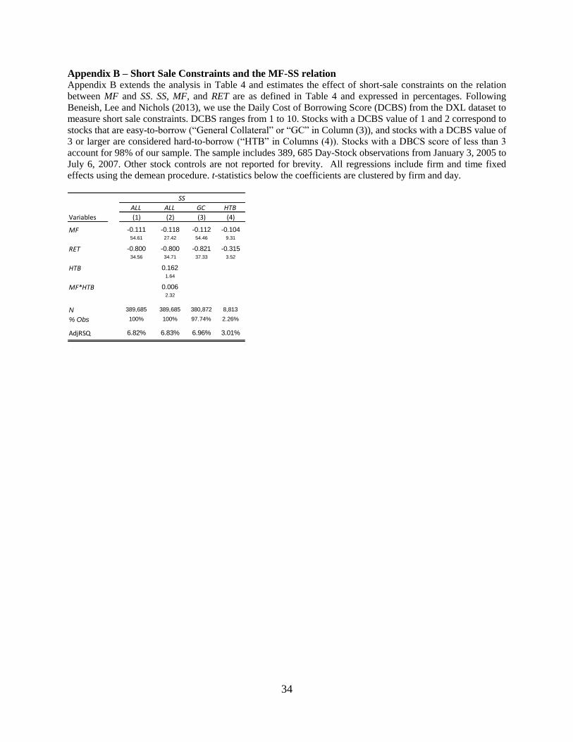
34

Appendix B – Short Sale Constraints and the MF-SS relation Appendix B extends the analysis in Table 4 and estimates the effect of short-sale constraints on the relation

between MF and SS. SS, MF, and RET are as defined in Table 4 and expressed in percentages. Following

Beneish, Lee and Nichols (2013), we use the Daily Cost of Borrowing Score (DCBS) from the DXL dataset to

measure short sale constraints. DCBS ranges from 1 to 10. Stocks with a DCBS value of 1 and 2 correspond to

stocks that are easy-to-borrow (“General Collateral” or “GC” in Column (3)), and stocks with a DCBS value of

3 or larger are considered hard-to-borrow (“HTB” in Columns (4)). Stocks with a DBCS score of less than 3

account for 98% of our sample. The sample includes 389, 685 Day-Stock observations from January 3, 2005 to

July 6, 2007. Other stock controls are not reported for brevity. All regressions include firm and time fixed

effects using the demean procedure. t-statistics below the coefficients are clustered by firm and day.

SS

ALL ALL GC HTB

Variables (1) (2) (3) (4)

MF -0.111 -0.118 -0.112 -0.10454.61 27.42 54.46 9.31

RET -0.800 -0.800 -0.821 -0.31534.56 34.71 37.33 3.52

HTB 0.1621.64

MF*HTB 0.0062.32

N 389,685 389,685 380,872 8,813

% Obs 100% 100% 97.74% 2.26%

AdjRSQ 6.82% 6.83% 6.96% 3.01%

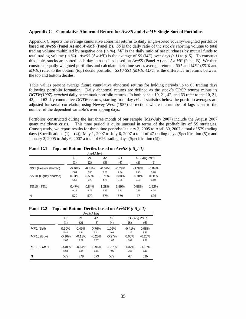
35

Appendix C – Cumulative Abnormal Return for AveSS and AveMF Single-Sorted Portfolios

Appendix C reports the average cumulative abnormal returns to daily single-sorted equally-weighted portfolios

based on AveSS (Panel A) and AveMF (Panel B). SS is the daily ratio of the stock’s shorting volume to total

trading volume multiplied by negative one (in %). MF is the daily ratio of net purchases by mutual funds to

total trading volume (in %). AveSS (AveMF) is the average of SS (MF) over days (t-1) to (t-5). To construct

this table, stocks are sorted each day into deciles based on AveSS (Panel A) and AveMF (Panel B). We then

construct equally-weighted portfolios and calculate their time-series average returns. SS1 and MF1 (SS10 and

MF10) refer to the bottom (top) decile portfolio. SS10-SS1 (MF10-MF1) is the difference in returns between

the top and bottom deciles.

Table values present average future cumulative abnormal returns for holding periods up to 63 trading days

following portfolio formation. Daily abnormal returns are defined as the stock’s CRSP returns minus its

DGTW(1997)-matched daily benchmark portfolio returns. In both panels 10, 21, 42, and 63 refer to the 10, 21,

42, and 63-day cumulative DGTW returns, starting from day t+1. t-statistics below the portfolio averages are

adjusted for serial correlation using Newey-West (1987) correction, where the number of lags is set to the

number of the dependent variable’s overlapping days.

Portfolios constructed during the last three month of our sample (May-July 2007) include the August 2007

quant meltdown crisis. This time period is quite unusual in terms of the profitability of SS strategies.

Consequently, we report results for three time periods: January 3, 2005 to April 30, 2007 a total of 579 trading

days (Specifications (1) – (4)); May 1, 2007 to July 6, 2007 a total of 47 trading days (Specification (5)); and

January 3, 2005 to July 6, 2007 a total of 626 trading days (Specification (6)).

Panel C.1 – Top and Bottom Deciles based on AveSS (t-5_t-1)

Panel C.2 – Top and Bottom Deciles based on AveMF (t-5_t-1)

AveSS Sort AveMF Sort

10 21 42 63 63 - Aug 2007

(1) (2) (3) (4) (5) (6)

SS1 (Heavily shorted) -0.16% -0.31% -0.57% -0.79% -1.39% -0.84%2.64 2.83 2.99 2.94 2.45 3.28

SS10 (Lightly shorted) 0.31% 0.53% 0.71% 0.80% -0.81% 0.68%5.50 6.22 4.75 3.85 2.63 3.10

SS10 - SS1 0.47% 0.84% 1.28% 1.59% 0.58% 1.52%6.15 6.75 7.12 5.72 0.89 4.08

N 579 579 579 579 47 626

AveMF Sort

10 21 42 63 63 - Aug 2007

(1) (2) (3) (4) (5) (6)

MF1 (Sell) 0.30% 0.46% 0.76% 1.09% -0.41% 0.98%5.82 4.34 3.11 3.63 1.26 3.33

MF10 (Buy) -0.10% -0.18% -0.20% -0.27% 0.66% -0.20%2.07 2.27 1.67 1.87 2.02 1.26

MF10 - MF1 -0.40% -0.64% -0.96% -1.37% 1.07% -1.18%6.63 6.24 5.51 7.05 1.66 5.13

N 579 579 579 579 47 626

36

References

Admati, A. R., 1985, A noisy rational expectations equilibrium for multi-asset securities markets,

Econometrica 53, 629-657.

Alexander, G. J., and M. A. Peterson, 2007, An analysis of trade-size clustering and its relation to stealth

trading, Journal of Financial Economics 84, 435-471.

Anand, A., Irvine, P., Puckett, A., Venkataraman, K., 2012, Performance of institutional trading desks: an

analysis of persistence in trading costs, Review of Financial Studies 25, 557–598.

Anand, A., Irvine, P., Puckett, A., Venkataraman, K., 2013, Institutional trading and stock resiliency:

Evidence from the 2007-2009 financial crisis, Journal of Financial Economics 108, 773–797.

Arif, S. and C. M. C. Lee, 2014, Aggregate investment and investor sentiment, Review of Financial

Studies, forthcoming.

Baker, M., and J. Wurgler, 2000, The equity share in new issues and aggregate stock returns, Journal of

Finance 55, 2219-2257.

Beneish, M., Lee, C. M. C., and D. C., Nichols, 2013, In short supply: Equity Overvaluation and Short

Selling, Indiana University, Syracuse University, and Stanford University working paper,

November.

Ben-David, I., F. Franzoni, and R. Moussawi. 2012. Hedge fund stock trading in the financial crisis of

2007–2008. Review of Financial Studies 25:1–54.

Ben-Rephael, A., S. Kandel, and A. Wohl, 2011, The price impact of aggregate mutual fund flows,

Journal of Financial and Quantitative Economics 46, 585-603.

__________________. 2012, Measuring investor sentiment with mutual fund flows, Journal of Financial

Economics 104, 363-382.

Boehmer, E., C. Jones and X. Zhang, 2008, Which Shorts are Informed? Journal of Finance 63, 491-527.

__________________. 2012. Shackling short sellers: The 2008 shorting ban. Working Paper, Singapore

Management University, Columbia Business School, and Purdue University.

__________________. 2013. What do short sellers know? Working Paper, Singapore Management

University, Columbia Business School, and Purdue University.

Boehmer, E., Z. R. Huszar and B. D. Jordan, 2010, The good news in short interest, Journal of Financial

Economics 96, 80-97.

Boehmer, E., and J. J. Wu, 2013, Short selling and the price discovery process, Review of Financial

Studies 26(2), 287-322.

Bris, A., W. N. Goetzmann, and N. Zhu, 2007, Efficiency and the Bear: Short sales and markets around

the world, Journal of Finance 62(3), 1029-1079.

Brunnermeier, M., and L. Pedersen, 2005, Predatory trading, Journal of Finance 60, 1825-1863.

37

Carhart, M. M., R. Kaniel, D. K. Musto, and A. V. Reed, 2002, Leaning for the Tape: Evidence of

Gaming Behavior in Equity Mutual Funds, Journal of Finance 57, 661-693.

Chakravarty, S., 2001, Stealth-trading: which traders’ trades move stock prices? Journal of Financial

Economics 61, 289-307.

Chemmanur, T. J., S. He, and G. Hu, 2009, The Role of Institutional Investors in Seasoned Equity

Offerings, Journal of Financial Economics 94, 384–411.

Chen, H., H. Desai, and S. Krishnamurthy, 2013, A first look at mutual funds that use short sales, Journal

of Financial and Quantitative Analysis 48(3), 761-787.

Chen, J., S. Hanson, H. Hong, and J. Stein, 2008, Do Hedge Funds Profit from Mutual Fund Distress?

NBER Working Paper 13786, February.

Christophe, S., M. Ferri, and J. Angel, 2004, Short-Selling Prior to Earnings Announcements, Journal of

Finance 59, 1845-1875.

Christophe, S., Ferri, M., Hsieh, J., 2010, Informed trading before analyst downgrades: evidence from

short sellers, Journal of Financial Economics 95, 85–106.

Coval, J., and E. Stafford, 2007, Asset fire sales (and purchases) in equity markets, Journal of Financial

Economics 86, 479-512.

Daniel, K., M. Grinblatt, S. Titman, and R. Wermers, 1997, Measuring Mutual Fund Performance with

Characteristic-Based Benchmarks, Journal of Finance 52, 1035-1058.

Daouk, H., C. M. C. Lee, and D. Ng, 2006, Capital market governance: how do security laws affect

market performance? Journal of Corporate Finance 12, 560-593.

Dechow, P. M., A. P. Hutton, L. Meulbroek, and R. G. Sloan, 2001, Short-sellers, fundamental analysis,

and stock returns. Journal of Financial Economics 61 (1), 77–106.

Del Guercio, D., and J. Reuter, 2014, Mutual fund performance and the incentive to generate alpha,

Journal of Finance, forthcoming.

Diamond, D. W., and R. E. Verrecchia, 1981, Information aggregation in noisy rational expectations

model, Journal of Financial Economics 9, 221-235.

Diether, K., Lee, K., and I. Werner, 2009, Short-Sale Strategies and Return Predictability, Review of

Financial Studies 22, 575-607.

Dichev, I., 2007, What Are Stock Investors’ Actual Historical Returns? Evidence from Dollar-Weighted

Returns, American Economic Review 97(1), 386-401.

Drake, M. S., L. Rees, and E. P. Swanson, 2011, Should Investors Follow the Prophets or the Bears?

Evidence on the Use of Public Information by Analysts and Short Sellers, The Accounting Review

86, 101-130.

38

Dyakov, T. and M. Verbeek, 2013, Front-running of mutual fund fire-sales, Journal of Banking &

Finance 37(12), 4931-4942.

Engelberg, J. E., A. V. Reed, and M. C. Ringgenberg, 2012, How are shorts informed? Short sellers,

news, and information processing, Journal of Financial Economics 105, 260-278.

Evans, R., C. Geczy, D. Musto, and A. Reed, 2009, Failure is an Option: Impediments to Short-Selling

and Options Prices, Review of Financial Studies 22(5),

Fama, Eugene F., and French, Kenneth R., 2010, Luck versus skill in the cross-section of mutual fund

returns, Journal of Finance 65, 1915–1947.

Fama, Eugene F., and James D. MacBeth, 1973, Risk, return, and equilibrium: Empirical tests, Journal of

Political Economy 81, 607-636.

French, Kenneth R., 2008, The cost of active investing, Journal of Finance 63, 1537–1573.

Franzoni, F., and A. Plazzi, 2012, Hedge Funds’ Liquidity Provision and Trading Activity, University of

Lugano and Swiss Finance Institute Working Paper, November.

Frazzini, A., and O. Lamont, 2008, “Dumb money: Mutual Fund Flows and the Cross-Section of Stock

Returns”, Journal of Financial Economics 88(2), 299-322.

Gantchev, N., and C. Jotikasthira, 2013. Hedge Fund Activists: Do They Take Cues from Institutional

Exit? Working paper.

Goldman Sachs. 2008. Goldman Sachs hedge fund trend monitor. February 20.

Goldstein, M. A., P. Irvine, and A. Puckett, 2011, Purchasing IPOs with commissions, Journal of

Financial and Quantitative Analysis 46, 1193-1225.

Griffin, J. M., and J. Xu, 2009, How smart are the smart guys? A unique view from hedge fund stock

holdings, Review of Financial Studies 22, 2531-2570.

Grinblatt, M., S. Titman, and R. Wermers, 1995, Momentum investment strategies, portfolio

performance, and herding: A study of mutual fund behavior, American Economic Review 85,

1088–1105.

Gruber, Martin J., 1996, Another puzzle: The growth in actively managed mutual funds, Journal of

Finance 51, 783–810.

Harris, M. and A. Raviv, 1993, Differences of opinion make a horse race, Review of Financial Studies 6,

473-506.

Hanson, S. G., and A. Sunderam. 2014. The growth and limits of arbitrage: evidence from short interest,

Review of Financial Studies 27 (4), 1238-1286.

Hong, H., and J. C. Stein, 2007, Disagreement and the stock market, Journal of Economic Perspectives

21:2, 109-128.

39

Jame, R., 2012, Pension Fund Trading and Stock Returns, University of New South Wales working paper,

May.

, 2013, How do hedge fund “stars” create value? Evidence from their daily trades,

University of New South Wales working paper, June.

Kandel, E., and N. D. Pearson, 1995, Differential interpretation of public signals and trade in speculative

markets, Journal of Political Economy 103, 831-872.

Karpoff, J., and X. Lou, 2010, Short sellers and financial misconduct, Journal of Finance 65 (5), 1879–

1913.

Khan, M., L. Kogan, and G. Serafeim, 2012, Mutual Fund Trading Pressure: Firm-Level Stock Price

Impact and Timing of SEOs, Journal of Finance 67 (4), 1371-1395.

Khan, M. and H. Lu, 2013, Do short sellers front-run insider sales? The Accounting Review, 88(5), 1743-

1768.

Lehmann, B. N., 1990, Fads, martingales, and market efficiency, Quarterly Journal of Economics 105, 1–

28.

Lou, D., 2012, A flow-based explanation for return predictability, Review of Financial Studies 25(1),

3457-3489.

Nagel, S., 2012, Evaporating liquidity, Review of Financial Studies 25:7, 2005-2039.

Newey, W. K. and K. D. West, 1987, A Simple, Positive Semi-Definite, Heteroskedasticity and

Autocorrelation Consistent Covariance Matrix, Econometrica 55, 703–708.

Puckett, A., X. Yan, 2011, The interim trading skills of institutional investors, Journal of Finance 66,

601–633.

, 2013, Short-term institutional herding and its impact on stock prices, University of

Missouri working paper.

Sharpe, W., F., 1991, The arithmetic of active management, Financial Analysts Journal 47:1,

January/February, 7-9.

Shive, S. and H. Yun, 2013, Are mutual funds sitting ducks? Journal of Financial Economics 107, 220-

237

So, E. C., and S. Wang, 2014, News-driven return reversals: liquidity provision ahead of earnings

announcements, Journal of Financial Economics, forthcoming.

Stambaugh, R. F., J. Yu, and Y. Yuan, 2012. The short of it: Investor sentiment and anomalies, Journal

of Financial Economics 104(2), 288-302.

Stefanini, F., 2006, Investment strategies of hedge funds, John Wiley & Sons Ltd., West Sussex, England.

40

Varian, H., R., 1989, Differences of opinion in financial markets, in CC. Stone, ed., Financial risk:

theory, evidence and implications: Proceedings of the 11th annual economic policy conference of

the Federal Reserve Bank of St. Louis, Kluwer Academic Publishers, Boston MA.

Verrecchia, R., 1982, Information acquisition in a noisy rational expectations economy, Econometrica 50,

1415-1430.

Table 1 – Summary Statistics of Main Variables

This table reports the time-series averages of the daily cross-sectional statistics for our main variables. The

sample consists of daily observations from January 3, 2005 to July 6, 2007, a total of 626 trading days. Panel

1.A reports summary statistics for key variables, each expressed as a percentage of daily total trading volume

for each stock. SS is the total number of shares traded in short-seller initiated transactions multiplied by

negative one. MF is net directional trading by mutual funds, computed as the daily total shares purchased

minus shares sold across all MFs in our sample. AbsMF is the absolute value of MF, and provides a sense of

the absolute magnitude of daily MF directional trading. MF Vol is daily total mutual fund trading volume

(buys plus sells). Panel 1.B examines the directional concordance/discordance of daily MF and SS trades. To

construct this panel, we first demean SS at the firm-level (i.e. control for the average firm-level SS). We then

group each firm-day observation by the sign of MF and the demeaned SS value independently. Table values in

Panel 1.B represent the percentage of firm-day observations in each category, where “SS Buys” refer to days

when SS-initiated volume is below firm-level mean, and “SS Sells” refer to days when SS-initated volume is

above firm-level mean.

Panel 1.A Descriptive Statistics

Panel 1.B Directional Concordance/Discordance

MF Buys MF Sells

“SS Buys” 26.0% 28.3% 54.3%

“SS Sells” 28.0% 17.7% 45.7%

54.0%

46.0%

Total Disagree 56.5% Total Agree 43.5%

Variables Mean Median SD

As Percentage of Daily Share Volume

SS -18.79 -17.48 9.01

MF 0.29 0.19 14.08

AbsMF 9.28 4.79 11.62

MF Vol 13.65 8.62 14.85

As Percentage of Outstanding Shares

SS_SHR -0.164 -0.108 0.166

MF_SHR 0.000 0.001 0.128

AbsMF_SHR 0.080 0.030 0.152

MF Vol_SHR 0.118 0.053 0.206

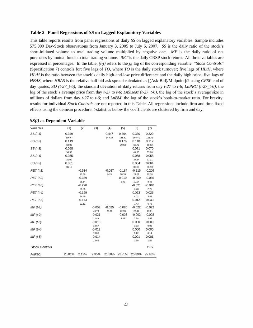
41

Table 2 –Panel Regressions of SS on Lagged Explanatory Variables

This table reports results from panel regressions of daily SS on lagged explanatory variables. Sample includes

575,000 Day-Stock observations from January 3, 2005 to July 6, 2007. SS is the daily ratio of the stock’s

short-initiated volume to total trading volume multiplied by negative one. MF is the daily ratio of net

purchases by mutual funds to total trading volume. RET is the daily CRSP stock return. All three variables are

expressed in percentages. In the table, (t-j) refers to the jth lag of the corresponding variable. “Stock Controls”

(Specification 7) controls for: five lags of TO, where TO is the daily stock turnover; five lags of HLtH, where

HLtH is the ratio between the stock’s daily high-and-low price difference and the daily high price; five lags of

HBAS, where HBAS is the relative half bid-ask spread calculated as [(Ask-Bid)/Midpoint]/2 using CRSP end of

day quotes; SD (t-27_t-6), the standard deviation of daily returns from day t-27 to t-6; LnPRC (t-27_t-6), the

log of the stock’s average price from day t-27 to t-6; LnSizeM (t-27_t-6), the log of the stock’s average size in

millions of dollars from day t-27 to t-6; and LnBM, the log of the stock’s book-to-market ratio. For brevity,

results for individual Stock Controls are not reported in this Table. All regressions include firm and time fixed

effects using the demean procedure. t-statistics below the coefficients are clustered by firm and day.

SS(t) as Dependent Variable

Variables (1) (2) (3) (4) (5) (6) (7)

SS (t-1) 0.349 0.447 0.364 0.330 0.329136.57 143.25 138.32 168.41 128.41

SS (t-2) 0.119 0.176 0.118 0.11760.92 79.53 69.72 58.52

SS (t-3) 0.068 0.071 0.07036.50 41.30 35.66

SS (t-4) 0.055 0.058 0.05831.00 34.34 31.11

SS (t-5) 0.061 0.064 0.06436.10 39.06 36.13

RET (t-1) -0.514 -0.087 -0.184 -0.215 -0.20940.30 9.15 18.35 24.07 20.10

RET (t-2) -0.359 0.010 -0.069 -0.06635.14 1.43 10.54 8.43

RET (t-3) -0.270 -0.021 -0.01831.35 3.48 2.75

RET (t-4) -0.199 0.023 0.02624.49 4.02 3.88

RET (t-5) -0.173 0.042 0.04322.11 7.43 6.75

MF (t-1) -0.059 -0.025 -0.020 -0.022 -0.02249.73 26.21 22.70 25.44 23.91

MF (t-2) -0.021 -0.003 -0.002 -0.00222.43 3.42 2.58 2.55

MF (t-3) -0.013 0.000 0.00013.67 0.13 0.03

MF (t-4) -0.012 0.000 0.00013.85 0.22 0.14

MF (t-5) -0.014 0.001 0.00113.62 1.60 1.54

Stock Controls YES

AdjRSQ 25.01% 2.12% 2.35% 21.30% 23.75% 25.39% 25.48%

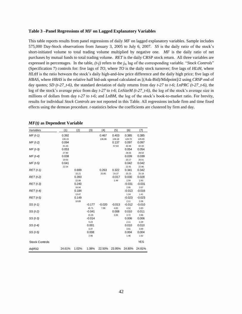
42

Table 3 –Panel Regressions of MF on Lagged Explanatory Variables

This table reports results from panel regressions of daily MF on lagged explanatory variables. Sample includes

575,000 Day-Stock observations from January 3, 2005 to July 6, 2007. SS is the daily ratio of the stock’s

short-initiated volume to total trading volume multiplied by negative one. MF is the daily ratio of net

purchases by mutual funds to total trading volume. RET is the daily CRSP stock return. All three variables are

expressed in percentages. In the table, (t-j) refers to the jth lag of the corresponding variable. “Stock Controls”

(Specification 7) controls for: five lags of TO, where TO is the daily stock turnover; five lags of HLtH, where

HLtH is the ratio between the stock’s daily high-and-low price difference and the daily high price; five lags of

HBAS, where HBAS is the relative half bid-ask spread calculated as [(Ask-Bid)/Midpoint]/2 using CRSP end of

day quotes; SD (t-27_t-6), the standard deviation of daily returns from day t-27 to t-6; LnPRC (t-27_t-6), the

log of the stock’s average price from day t-27 to t-6; LnSizeM (t-27_t-6), the log of the stock’s average size in

millions of dollars from day t-27 to t-6; and LnBM, the log of the stock’s book-to-market ratio. For brevity,

results for individual Stock Controls are not reported in this Table. All regressions include firm and time fixed

effects using the demean procedure. t-statistics below the coefficients are clustered by firm and day.

MF(t) as Dependent Variable

Variables (1) (2) (3) (4) (5) (6) (7)

MF (t-1) 0.392 0.467 0.403 0.385 0.385130.15 136.88 136.18 129.70 129.49

MF (t-2) 0.094 0.137 0.097 0.09741.33 57.63 42.36 42.33

MF (t-3) 0.053 0.054 0.05427.90 28.55 28.54

MF (t-4) 0.038 0.039 0.03919.53 20.17 20.01

MF (t-5) 0.041 0.042 0.04222.54 22.91 22.86

RET (t-1) 0.699 0.263 0.322 0.341 0.34233.21 20.85 24.37 25.23 25.18

RET (t-2) 0.393 -0.017 0.030 0.02822.99 1.49 2.59 2.93

RET (t-3) 0.240 -0.031 -0.03116.94 2.95 2.07

RET (t-4) 0.184 -0.013 -0.01613.47 1.24 1.41

RET (t-5) 0.149 -0.023 -0.02310.89 2.11 2.06

SS (t-1) -0.177 -0.020 -0.013 -0.012 -0.01045.71 7.88 4.83 4.52 3.83

SS (t-2) -0.041 0.008 0.010 0.01115.35 3.06 3.72 3.96

SS (t-3) -0.014 0.006 0.0065.23 2.11 2.29

SS (t-4) 0.001 0.010 0.0100.37 3.61 3.69

SS (t-5) 0.008 0.004 0.0042.96 1.46 1.62

Stock Controls YES

AdjRSQ 24.61% 1.02% 1.38% 22.50% 23.95% 24.80% 24.81%

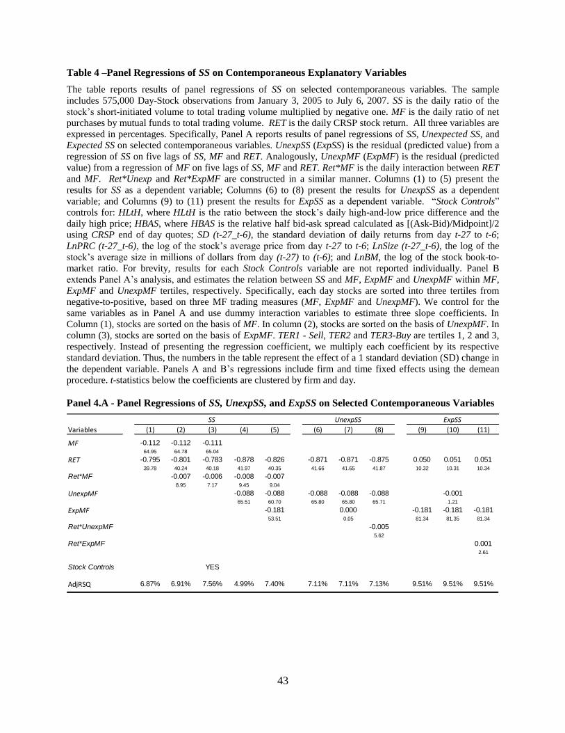
43

Table 4 –Panel Regressions of SS on Contemporaneous Explanatory Variables

The table reports results of panel regressions of SS on selected contemporaneous variables. The sample

includes 575,000 Day-Stock observations from January 3, 2005 to July 6, 2007. SS is the daily ratio of the

stock’s short-initiated volume to total trading volume multiplied by negative one. MF is the daily ratio of net

purchases by mutual funds to total trading volume. RET is the daily CRSP stock return. All three variables are

expressed in percentages. Specifically, Panel A reports results of panel regressions of SS, Unexpected SS, and Expected SS on selected contemporaneous variables. UnexpSS (ExpSS) is the residual (predicted value) from a

regression of SS on five lags of SS, MF and RET. Analogously, UnexpMF (ExpMF) is the residual (predicted

value) from a regression of MF on five lags of SS, MF and RET. Ret*MF is the daily interaction between RET

and MF. Ret*Unexp and Ret*ExpMF are constructed in a similar manner. Columns (1) to (5) present the

results for SS as a dependent variable; Columns (6) to (8) present the results for UnexpSS as a dependent

variable; and Columns (9) to (11) present the results for ExpSS as a dependent variable. “Stock Controls”

controls for: HLtH, where HLtH is the ratio between the stock’s daily high-and-low price difference and the

daily high price; HBAS, where HBAS is the relative half bid-ask spread calculated as [(Ask-Bid)/Midpoint]/2

using CRSP end of day quotes; SD (t-27_t-6), the standard deviation of daily returns from day t-27 to t-6;

LnPRC (t-27_t-6), the log of the stock’s average price from day t-27 to t-6; LnSize (t-27_t-6), the log of the

stock’s average size in millions of dollars from day (t-27) to (t-6); and LnBM, the log of the stock book-to-

market ratio. For brevity, results for each Stock Controls variable are not reported individually. Panel B

extends Panel A’s analysis, and estimates the relation between SS and MF, ExpMF and UnexpMF within MF,

ExpMF and UnexpMF tertiles, respectively. Specifically, each day stocks are sorted into three tertiles from

negative-to-positive, based on three MF trading measures (MF, ExpMF and UnexpMF). We control for the

same variables as in Panel A and use dummy interaction variables to estimate three slope coefficients. In

Column (1), stocks are sorted on the basis of MF. In column (2), stocks are sorted on the basis of UnexpMF. In

column (3), stocks are sorted on the basis of ExpMF. TER1 - Sell, TER2 and TER3-Buy are tertiles 1, 2 and 3,

respectively. Instead of presenting the regression coefficient, we multiply each coefficient by its respective

standard deviation. Thus, the numbers in the table represent the effect of a 1 standard deviation (SD) change in

the dependent variable. Panels A and B’s regressions include firm and time fixed effects using the demean

procedure. t-statistics below the coefficients are clustered by firm and day.

Panel 4.A - Panel Regressions of SS, UnexpSS, and ExpSS on Selected Contemporaneous Variables

SS UnexpSS ExpSS

Variables (1) (2) (3) (4) (5) (6) (7) (8) (9) (10) (11)

MF -0.112 -0.112 -0.11164.95 64.78 65.04

RET -0.795 -0.801 -0.783 -0.878 -0.826 -0.871 -0.871 -0.875 0.050 0.051 0.05139.78 40.24 40.18 41.97 40.35 41.66 41.65 41.87 10.32 10.31 10.34

Ret*MF -0.007 -0.006 -0.008 -0.0078.95 7.17 9.45 9.04

UnexpMF -0.088 -0.088 -0.088 -0.088 -0.088 -0.00165.51 60.70 65.80 65.80 65.71 1.21

ExpMF -0.181 0.000 -0.181 -0.181 -0.18153.51 0.05 81.34 81.35 81.34

Ret*UnexpMF -0.0055.62

Ret*ExpMF 0.0012.61

Stock Controls YES

AdjRSQ 6.87% 6.91% 7.56% 4.99% 7.40% 7.11% 7.11% 7.13% 9.51% 9.51% 9.51%

44

Panel 4.B – MF effect by Flow Tertiles

Dependent Variable SS

Exp. Sorting Variables MF ExpMF UnexpMF

Sorting Tertiles (1) (2) (3)

TER 1 - Sell -1.613 -1.010 -1.33663.56 38.76 58.67

TER 2 -0.183 -0.197 -0.0608.41 9.61 3.35

TER 3 - Buy -0.430 -0.576 -0.26911.38 16.98 4.58

45

Table 5 – MF, SS and Short-Term Future Stock Returns The table reports results of short-term future returns analyses using single sorted portfolios (Panel A) and

Fama-Macbeth (1973) cross-sectional regressions (Panel B) from January 3, 2005 to July 6, 2007, a total of

626 trading days. RET is the daily CRSP stock return (in %). DGTW is the stock return (RET) minus the

DGTW (1997)-matched daily benchmark portfolio return. SS is the daily ratio of the stock’s shorting volume to

total trading volume multiplied by negative one (in %). MF is the daily ratio of net purchases by mutual funds

to total trading volume (in %).

Panel A presents results of single sorted portfolios based on previous day DGTW adjusted returns. Specifically,

stocks are sorted each day into deciles based on day t’s DGTW-adjusted abnormal returns. We then construct

equally-weighted portfolios and calculate their time-series average returns. DGTW1-Losers (DGTW10-

Winners) refers to the bottom (top) decile portfolio. D10-D1 is the difference in returns between the top and

bottom deciles. MF Decile Rank (SS Decile Rank) is the average decile rank of the stock when ranked on MF

(SS). Specifically, each day stocks are independently sorted into deciles based on day t MF (SS). The table then

reports the MF (SS) average decile rank of stocks in the top and bottom DGTW portfolios.

Panel B presents results of daily Fama-Macbeth (1973) cross-sectional regressions of cumulative DGTW

adjusted stock returns from day t+1 to t+10 on day-t explanatory variables. All coefficients are multiplied by

100 for ease of presentation. UnexpMF (ExpMF) is the residual (predicted value) from a regression of MF on

five lags of SS, MF and RET. SS*ExpMF (SS*UnexpMF) is the daily interaction between SS and ExpMF

(UnexpMF). All other interaction terms are constructed in a similar manner. Stock Controls are the same

controls used in Table 2. t-statistics below the coefficients are adjusted for serial correlation using the Newey-

West (1987) correction, where the number of lags is set to the number of the dependent variable’s overlapping

days.

Panel 5.A – Top and Bottom Deciles based on DGTW (t)

Panel 5.B - Cross Sectional Regressions of Cumulative DGTW on day-t Explanatory Variables

Dgtw t+1 MF Decile Rank SS Decile Rank

(1) (2) (3)

Dgtw 1 - Losers 0.060% 4.84 6.053.68

Dgtw 10 - Winners -0.045% 6.07 4.293.12

D10 - D1 -0.105% 1.23 *** -1.75 ***4.00

DGTW t+1 DGTW t+1_t+2 DGTW t+1_t+3 DGTW t +1_t +5 DGTW t +1_t +10

Variables - time t (1) (2) (3) (4) (5) (6) (7) (8) (9) (10)

DGTW -1.818 -1.514 -1.617 -1.115 -1.794 -1.171 -1.302 -0.446 0.985 2.2884.42 3.63 2.78 1.89 2.64 1.70 1.55 0.52 0.82 1.83

ExpMF -0.095 -0.187 -0.214 -0.318 -0.332 -0.463 -0.552 -0.689 -1.132 -1.5802.97 2.81 4.06 2.91 4.76 3.14 5.27 3.10 6.03 4.90

UnexpMF 0.071 0.081 0.082 0.068 0.077 0.056 0.049 0.011 -0.149 -0.2643.90 1.95 2.88 1.21 2.17 0.80 0.51 0.12 2.69 2.02

SS 0.410 0.619 0.763 1.036 1.61412.34 11.95 10.88 9.50 9.19

SS*ExpMF -0.010 -0.012 -0.016 -0.018 -0.0412.98 2.36 2.21 2.15 3.14

SS*UnexpMF -0.002 -0.004 -0.005 -0.008 -0.0150.71 1.42 1.59 1.78 2.21

Stock Controls Yes Yes Yes Yes Yes Yes Yes Yes Yes Yes

AdjRSQ 3.24% 3.41% 3.27% 3.43% 3.13% 3.27% 2.97% 3.13% 2.70% 2.86%

46

Table 6 – Panel Regressions of SS and MF averaged over 5 days on Lagged Explanatory Variables

This table reports results from panel regressions of SS (Panel A) and MF (Panel B) averaged over 5 days on lagged

explanatory variables. Sample includes 575,000 Day-Stock observations from January 3, 2005 to July 6, 2007.

AveSS (t_t+4) is defined as the average of SS(t) to SS(t+4). In a similar manner, the prefix “Ave” refers to the

average of the specified period. For example, Ave MF(t-5_t-1) is the average of MF(t-5) to MF(t-1). SS is the daily

ratio of the stock’s short-initiated volume to total trading volume multiplied by negative one. MF is the daily ratio

of net purchases by mutual funds to total trading volume. RET is the daily CRSP stock return. All three variables

are expressed in percentages. In the table, (t-j) refers to the jth lag of the corresponding variable. “Stock Controls”

(Specification 6) controls for: five lags of TO, where TO is the daily stock turnover; five lags of HLtH, where HLtH

is the ratio between the stock’s daily high-and-low price difference and the daily high price; five lags of HBAS,

where HBAS is the relative half bid-ask spread calculated as [(Ask-Bid)/Midpoint]/2 using CRSP end of day quotes;

SD (t-27_t-6), the standard deviation of daily returns from day t-27 to t-6; LnPRC (t-27_t-6), the log of the stock’s

average price from day t-27 to t-6; LnSizeM (t-27_t-6), the log of the stock’s average size in millions of dollars from

day t-27 to t-6; and LnBM, the log of the stock’s book-to-market ratio. All regressions include firm and time fixed

effects using the demean procedure. t-statistics below the coefficients are clustered by firm and day.

Panel 6.A – AveSS (t_t+4) as Dependent Variable

Variables (1) (2) (3) (4) (5) (6)

AveSS (t-5_t-1) 0.446 0.445 0.439 0.43195.17 91.77 88.23 88.65

AveRET (t-5_t-1) -0.731 -0.026 -0.005 0.02922.42 1.21 0.23 1.03

AveMF (t-5_t-1) -0.079 -0.016 -0.01631.79 8.92 8.88

AveTO (t-5_t-1) 10.3372.61

AveHLtH (t-5_t-1) -6.3051.85

SD (t-27_t-6) 15.7495.67

LnSizeM (t-27_t-6) 2.80012.03

LnBM 0.3512.98

AveHBAS (t-5_t-1) -3.7390.12

LnAvePRC (t-27_t-6) -0.9574.27

AdjRSQ 19.96% 0.86% 1.82% 19.96% 20.03% 20.49%

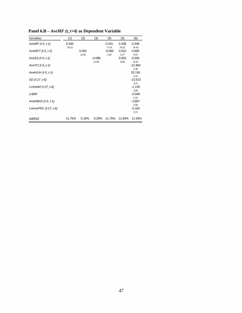
47

Panel 6.B – AveMF (t_t+4) as Dependent Variable

Variables (1) (2) (3) (4) (5) (6)

AveMF (t-5_t-1) 0.330 0.331 0.338 0.33878.15 77.41 78.22 78.43

AveRET (t-5_t-1) 0.562 -0.060 0.010 0.00012.82 1.62 0.27 0.01

AveSS (t-5_t-1) -0.088 0.053 0.05912.99 9.68 10.81

AveTO (t-5_t-1) -21.8624.36

AveHLtH (t-5_t-1) 25.7405.23

SD (t-27_t-6) -13.5233.07

LnSizeM (t-27_t-6) -1.1353.99

LnBM -0.0490.32

AveHBAS (t-5_t-1) -3.8570.08

LnAvePRC (t-27_t-6) -0.1820.72

AdjRSQ 11.75% 0.19% 0.29% 11.75% 11.84% 11.93%

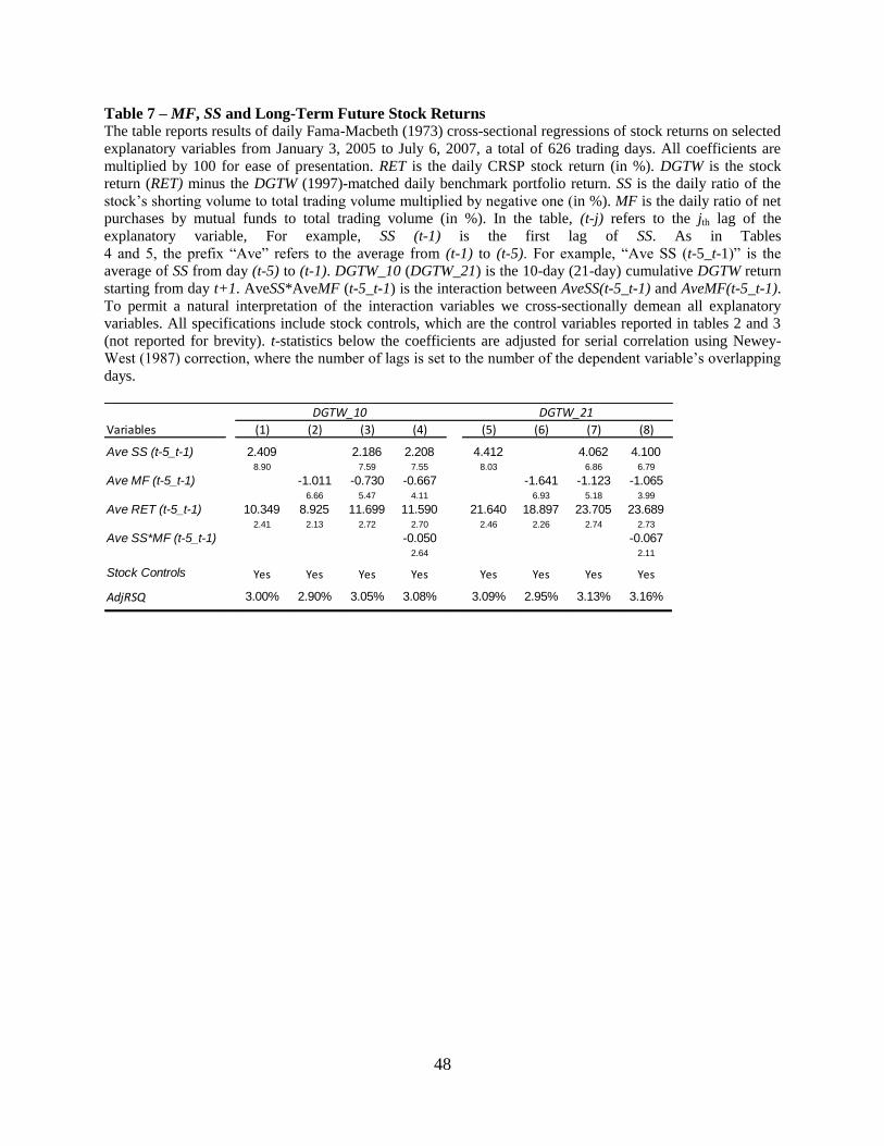
48

Table 7 – MF, SS and Long-Term Future Stock Returns The table reports results of daily Fama-Macbeth (1973) cross-sectional regressions of stock returns on selected

explanatory variables from January 3, 2005 to July 6, 2007, a total of 626 trading days. All coefficients are

multiplied by 100 for ease of presentation. RET is the daily CRSP stock return (in %). DGTW is the stock

return (RET) minus the DGTW (1997)-matched daily benchmark portfolio return. SS is the daily ratio of the

stock’s shorting volume to total trading volume multiplied by negative one (in %). MF is the daily ratio of net

purchases by mutual funds to total trading volume (in %). In the table, (t-j) refers to the jth lag of the

explanatory variable, For example, SS (t-1) is the first lag of SS. As in Tables

4 and 5, the prefix “Ave” refers to the average from (t-1) to (t-5). For example, “Ave SS (t-5_t-1)” is the

average of SS from day (t-5) to (t-1). DGTW_10 (DGTW_21) is the 10-day (21-day) cumulative DGTW return

starting from day t+1. AveSS*AveMF (t-5_t-1) is the interaction between AveSS(t-5_t-1) and AveMF(t-5_t-1).

To permit a natural interpretation of the interaction variables we cross-sectionally demean all explanatory

variables. All specifications include stock controls, which are the control variables reported in tables 2 and 3

(not reported for brevity). t-statistics below the coefficients are adjusted for serial correlation using Newey-

West (1987) correction, where the number of lags is set to the number of the dependent variable’s overlapping

days.

DGTW_10 DGTW_21

Variables (1) (2) (3) (4) (5) (6) (7) (8)

Ave SS (t-5_t-1) 2.409 2.186 2.208 4.412 4.062 4.1008.90 7.59 7.55 8.03 6.86 6.79

Ave MF (t-5_t-1) -1.011 -0.730 -0.667 -1.641 -1.123 -1.0656.66 5.47 4.11 6.93 5.18 3.99

Ave RET (t-5_t-1) 10.349 8.925 11.699 11.590 21.640 18.897 23.705 23.6892.41 2.13 2.72 2.70 2.46 2.26 2.74 2.73

Ave SS*MF (t-5_t-1) -0.050 -0.0672.64 2.11

Stock Controls Yes Yes Yes Yes Yes Yes Yes Yes

AdjRSQ 3.00% 2.90% 3.05% 3.08% 3.09% 2.95% 3.13% 3.16%

49

Table 8 – Cumulative Abnormal Return of Double-Sorted Portfolios based on AveSS

and AveMF

The table reports the average cumulative abnormal return to double-sorted portfolios in the 21, 42, and 63 trading

days after portfolio formation. To construct this table, firms are sorted independently into quintiles each day based

on AveMF(t-5_t-1) and AveSS(t-5_t-1), where MF1 and SS1 (MF5 and SS5) denote the firms with the lowest

(highest) values. SS is the daily ratio of the stock’s shorting volume to total trading volume multiplied by negative

one. MF is the daily ratio of net purchases by mutual funds to total trading volume. AveSS (AveMF) is the average of

SS (MF) over days t-5 to t-1. RET is the stock’s CRSP’s daily return. DGTW abnormal return is RET minus the

stock’s DGTW (1997)-matched daily benchmark portfolio return.

Panel A reports results for independent double-sorted portfolio. For each portfolio, we report the time series average

DGTW abnormal return, t-statistic, and average number of stocks. In both panels the headers, 21, 42, and 63 refer to

the 21, 42, and 63-day cumulative DGTW abnormal returns, starting from day t+1. Specifically, we use AveMF and

AveSS quintiles to construct 25 equally-weighted portfolios. We keep the top and bottom AveMF and AveSS

intersection quintile portfolios. For example, the intersection between MF1 and SS1 (denoted as MF1_SS1) is the

portfolio of firms in the lowest AveMF (MF1) and the lowest AveSS (SS1) quintiles.

Panel B reports results of portfolios which capture the wealth transfers between MF and SS. Specifically, “Disagree”

is the return difference between MF1_SS5 and MF5_SS1 portfolios, i.e. it represents the future DGTW return for a

cash-neutral portfolio of firms where MF and SS are trade in opposite directions. “Agree” is the return difference

between the MF5_SS5 and MF1_SS1 portfolios, i.e. where MF and SS trade in the same direction. “DMA” is the

Disagree-minus-Agree portfolio, which is the return difference between the “Disagree” and “Agree” portfolios.

For completeness, Panel C reports results for alternative strategies based on the information in Panel A. “Pure MF

portfolios” presents results for top-minus-bottom MF strategies (i.e., MF5-minus-MF1) conditioning on SS1 and SS5

quintiles. “Pure SS portfolios” provides results for top-minus-bottom SS strategies (SS5-minus-SS1) conditioning on

MF1 and MF5 quintiles.

To isolate the effect of the August 2007 ‘quant meltdown’, we report results for three separate time periods: The

pre-meltdown period, from January 3, 2005 to April 30, 2007, a total of 579 trading days (Specifications (1) – (3));

the meltdown period, May 1, 2007 to July 6, 2007 a total of 47 trading days (Specification (4)); and the total sample

period, from January 3, 2005 to July 6, 2007, a total of 626 trading days (Specification (5)).

t-statistics below the portfolio averages are adjusted for serial correlation using Newey-West (1987) correction,

where the number of lags is set to equal the overlap in the dependent variable.

Panel 8.A – MF and SS Independent Sort Quintile Portfolios

(1) (2) (3) (4) (5)

21 42 63 63 - Aug 2007

AveMF AveMF AveMF AveMF AveMF

MF1 MF5 MF1 MF5 MF1 MF5 MF1 MF5 MF1 MF5

AveSS

SS1 (Heavily shorted) -0.20 -0.33 -0.17 -0.57 -0.18 -0.84 -1.70 1.23 -0.29 -0.68

t-stat 1.21 3.55 0.57 3.89 1.24 4.32 3.39 4.32 2.10 3.23

Num Stocks 18 48 18 48 18 48 23 60 19 49

SS5 (Lightly shorted) 0.64 0.30 0.89 0.34 1.15 0.39 -0.63 -1.45 1.01 0.26

t-stat 4.02 3.01 4.23 1.96 4.15 1.99 4.15 2.38 3.64 2.79

Num Stocks 56 25 56 25 56 25 60 25 56 25

N 579 579 579 47 626

50

Panel 8.B – Disagree, Agree and the DMA (Disagree-minus-Agree) Portfolios

Panel 8.C – Returns to Alternative Strategies

(1) (2) (3) (4) (5)

21 42 63 63 - Aug 2007

Disagreement portfoio: 0.97 1.46 1.98 -1.86 1.69

MF1_SS5 minus MF5_SS1 4.13 3.98 4.32 4.13 3.71

Agreement portfolio: 0.50 0.51 0.57 0.25 0.55

MF5_SS5 minus MF1_SS1 1.99 2.55 1.96 0.38 2.00

DMA - Disagree-minus-Agree 0.47 0.95 1.41 -2.11 1.152.13 3.20 3.46 2.01 2.71

N 579 579 579 47 626

(1) (2) (3) (4) (5)

21 42 63 63 - Aug 2007

Pure MF portfolio (controlling for SS):MF5 minus MF1 within SS1 -0.13 -0.40 -0.66 2.94 -0.39

t-stat 0.83 1.82 1.98 3.21 1.06

MF5 minus MF1 within SS5 -0.34 -0.55 -0.75 -0.83 -0.76

t-stat 2.68 2.99 3.28 1.78 4.67

Pure SS portfolio (controlling for MF):SS5 minus SS1 within MF1 0.84 1.06 1.32 1.08 1.30

t-stat 3.70 3.54 3.76 2.34 5.00

SS5 minus SS1 within MF5 0.63 0.91 1.23 -2.69 0.94

t-stat 3.41 3.74 4.39 4.99 3.37

N 579 579 579 47 626

51

Table 9 – DMA Portfolio Returns based on MF Holdings, Variance of Change in Holdings and

other Selected Variables

The Table examines the effect of various firm characteristics on the returns to the Disagree-minus-Agree

portfolio (the DMA portfolio as defined in Table 8). In Panels A and B we evaluate the effect of MF holdings

(hereafter, “MFH”) and MF volatility of quarterly change in holding (hereafter, “MFSD”) on the magnitude of

DMA returns. MFH (Panel A) is the aggregate MF holdings of a given stock at the end of quarter t-1, scaled by

shares outstanding. MFSD (Panel B) is the standard deviation of aggregate MF quarterly changes in holdings

of a given stock based on quarters t-5 to t-1. Aggregate quarterly change in MF holdings is calculated

following Sias, Stark and Titman (2006) as the difference between total shares held by mutual funds at the

beginning of the quarter and total shares held by mutual funds at the end of the quarter divided by shares

outstanding (in %). Since size and institutional ownership are positively correlated, in Panels A and B, we first

sort stocks into tertiles based on their average daily market capitalization from day t-27 to t-6 (Size). Then,

within each Size tertile, we further sort stocks into tertiles by either MFH or MFSD. We then evaluate the

effect of directional concordance (or discordance) in MFs and SSs trades by focusing on the size of the DMA

returns. To construct Panels’ A and B DMA portfolios, within of each of the nine portfolios (i.e., Size-MFH

and Size-MFSD) we further sort the stocks based on AveSS and AveMF tertiles. We then keep the intersection

of the top and bottom tertiles

Panel C presents DMA portfolios results for tertile sub-samples based on four selected variables: MFH

(Specification 1), MFSD (Specification 2), Size (Specification 3) and Relative Spread (Specification 4).

Relative Spread is the average relative half bid-ask spread from day t-27 to t-6, calculated as [(Ask-

Bid)/Midpoint]/2 using CRSP end of day quotes. Specifically, each day stocks are sorted by the four variables

into tertiles. Then, within each tertile portfolio, stocks are further sorted into quintiles based on AveSS and

AveMF. “Diff- in-DMA” is the difference between the top (“3”) and the bottom (“1”) tertiles. t-statistics below

the portfolio averages are adjusted for serial correlation using Newey-West (1987) correction, where the

number of lags is set to equal the overlap in the dependent variable. The sample period covers January 3, 2005

to April 30, 2007, a total of 579 trading days.

Panel 9.A – DMA Portfolio Returns based on MFH, after controlling for Size

Panel 9.B – DMA Portfolio Returns based on MFSD, after controlling for Size

(1) (2) (3)

Size 1 Size 2 Size 3

MFH 1 2.13% 0.82% -1.12%2.65 1.88 1.41

MFH 3 2.21% 1.83% 1.04%2.04 1.93 2.61

(1) (2) (3)

Size 1 Size 2 Size 3

MFSD 1 0.70% 0.12% 0.21%1.02 0.51 0.75

MFSD 3 2.33% 1.90% 0.57%2.54 2.43 0.92

52

Panel 9.C – Diff in DMA Returns across Tertiles of Various Firm Characteristics

(1) (2) (3) (4)

MFH MFSD Size Relative Spread

1 3 1 3 1 3 1 3

DMA 1.19% 2.81% 0.80% 1.79% 2.58% -0.47% -0.74% 1.97%1.69 3.96 1.71 3.61 2.91 0.89 1.31 2.89

Diff -in -DMA 1.62% 0.99% -3.05% 2.71%1.77 1.64 2.88 2.87

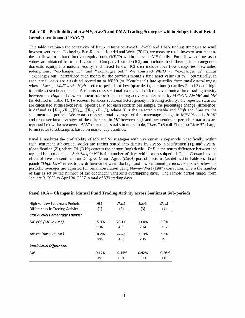
53

Table 10 – Profitability of AveMF, AveSS and DMA Trading Strategies within Subperiods of Retail

Investor Sentiment (“NEIO”)

This table examines the sensitivity of future returns to AveMF, AveSS and DMA trading strategies to retail

investor sentiment. Following Ben-Rephael, Kandel and Wohl (2012), we measure retail investor sentiment as

the net flows from bond funds to equity funds (NEIO) within the same MF family. Fund flows and net asset

values are obtained from the Investment Company Institute (ICI) and include the following fund categories:

domestic equity, international equity, and mixed funds. ICI data include four flow categories: new sales,

redemptions, ‘‘exchanges in,’’ and ‘‘exchanges out.’’ We construct NEIO as ‘‘exchanges in’’ minus

‘‘exchanges out’’ normalized each month by the previous month’s fund asset value (in %). Specifically, in

each panel, days are classified according to NEIO (or “Sentiment”) into quartiles from smallest-to-largest,

where “Low”, “Mid” and “High” refer to periods of low (quartile 1), medium (quartiles 2 and 3) and high

(quartile 4) sentiment. Panel A reports cross-sectional averages of differences in mutual fund trading activity

between the High and Low sentiment sub-periods. Trading activity is measured by MFVOL, AbsMF and MF

(as defined in Table 1). To account for cross-sectional heterogeneity in trading activity, the reported statistics

are calculated at the stock level. Specifically, for each stock in our sample, the percentage change (difference)

is defined as [XHigh-XLow]/XLow ([XHigh-XLow]), where X is the selected variable and High and Low are the

sentiment sub-periods. We report cross-sectional averages of the percentage change in MFVOL and AbsMF

and cross-sectional averages of the difference in MF between high and low sentiment periods. t-statistics are

reported below the averages. “ALL” refer to all stocks in our sample, “Size1” (Small Firms) to “Size 5” (Large

Firms) refer to subsamples based on market cap quintiles.

Panel B analyzes the profitability of MF and SS strategies within sentiment sub-periods. Specifically, within

each sentiment sub-period, stocks are further sorted into deciles by AveSS (Specification (1)) and AveMF

(Specification (2)), where D1 (D10) denotes the bottom (top) decile. TmB is the return difference between the

top and bottom deciles. “Sub Sample N” is the number of days within each subperiod. Panel C examines the

effect of investor sentiment on Disagree-Minus-Agree (DMA) portfolio returns (as defined in Table 8). In all

panels “High-Low” refers to the difference between the high and low sentiment periods. t-statistics below the

portfolio averages are adjusted for serial correlation using Newey-West (1987) correction, where the number

of lags is set by the number of the dependent variable’s overlapping days. The sample period ranges from

January 3, 2005 to April 30, 2007, a total of 579 trading days.

Panel 10.A – Changes in Mutual Fund Trading Activity across Sentiment Sub-periods

High vs. Low Sentiment Periods ALL Size1 Size3 Size5

Differences in Trading Activity (1) (2) (3) (4)

Stock Level Percentage Change:

MF VOL (MF volume) 15.9% 28.1% 13.4% 8.8%10.02 4.99 2.94 3.72

AbsMF (Absolute MF) 14.2% 24.4% 11.9% 5.8%

8.95 4.39 2.45 2.9

Stock Level Difference:

MF -0.17% -0.54% 0.42% -0.26%0.91 0.94 1.03 1.08

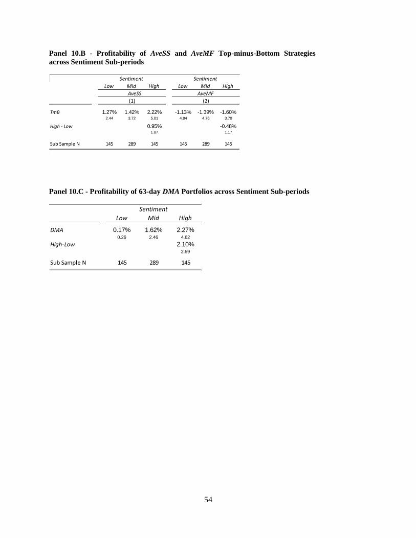
54

Panel 10.B - Profitability of AveSS and AveMF Top-minus-Bottom Strategies

across Sentiment Sub-periods

Panel 10.C - Profitability of 63-day DMA Portfolios across Sentiment Sub-periods

Sentiment Sentiment

Low Mid High Low Mid High

AveSS AveMF

(1) (2)

TmB 1.27% 1.42% 2.22% -1.13% -1.39% -1.60%2.44 3.72 5.01 4.84 4.76 3.70

High - Low 0.95% -0.48%1.87 1.17

Sub Sample N 145 289 145 145 289 145

Sentiment

Low Mid High

DMA 0.17% 1.62% 2.27%0.26 2.46 4.62

High-Low 2.10%2.59

Sub Sample N 145 289 145

55

Figure 1 – Daily Trading Patterns for MF and SS sorted on Top and Bottom MF flow deciles on

Day t

These figures depict daily trading patterns by mutual funds and short sellers, based on MF top and bottom

decile portfolios. MF is the daily ratio of net purchases by mutual funds to total trading volume (in %). SS is

the daily ratio of the stock’s shorting volume to total trading volume multiplied by negative one (in %).

Sample period is January 3, 2005 to July 6, 2007, a total of 626 trading days. Specifically, in all four graphs,

stocks are sorted into deciles based on MF on day t. Graphs 1.A and 1.B plot MF trades. Specifically, Graph

1.A reports the cross-sectional mean of MF each day from t-14 to t+63 and Graph 1.B reports the cumulative

cross-sectional averages of MF from Day t-14 to Day t+63. MF-Buy refers to the decile of stocks with the

most positive net MF trading on Day t (i.e. those with the largest net MF purchases). MF-Sell refers to the

decile of stocks with the most negative net MF trading on Day t (i.e. those stocks with the largest net MF

sales). Graphs 1.C and 1.D plot SS trades. Since SS is in terms of volume, both graphs present SS in terms of

deviations from the long-run mean. Graph 1.C reports the cross-sectional mean of SS deviations each day from

t-14 to t+63. Similarly, Graph 1.D reports the cumulative cross-sectional SS deviations from Day t-14 to Day

t+63.

Graph 1.A Graph 1.B

Daily MF for top and bottom MF Deciles Cumulative MF for top and bottom MF Deciles

Graph 1.C Graph 1.D

Daily Demeaned SS Cumulative Demeaned SS

for top and bottom MF Deciles for top and bottom MF Deciles

-30

-20

-10

0

10

20

30

-14 -10 -6 -2 2 6 10 14 18 22 26 30 34 38 42 46 50 54 58 62

Dai

ly M

Fin

%

Days

Daily MF ranked by MF on Day - 0

MF - Sell MF - Buy

-300

-200

-100

0

100

200

300

-14 -10 -6 -2 2 6 10 14 18 22 26 30 34 38 42 46 50 54 58 62

Cu

mu

lati

ve D

aily

MF

in %

Days

Cumulative MF ranked by MF on Day - 0

MF - Sell MF - Buy

-3

-2

-1

0

1

2

3

4

5

-14 -10 -6 -2 2 6 10 14 18 22 26 30 34 38 42 46 50 54 58 62

Dai

ly S

S in

%

Days

Daily Demeaned SS ranked by MF on Day - 0

MF - Sell MF - Buy

-30

-20

-10

0

10

20

30

-14 -10 -6 -2 2 6 10 14 18 22 26 30 34 38 42 46 50 54 58 62

Cu

mu

lati

ve D

aily

SS

in %

Days

Cumulative Daily Demeaned SS ranked by MF on Day - 0

MF - Sell MF - Buy

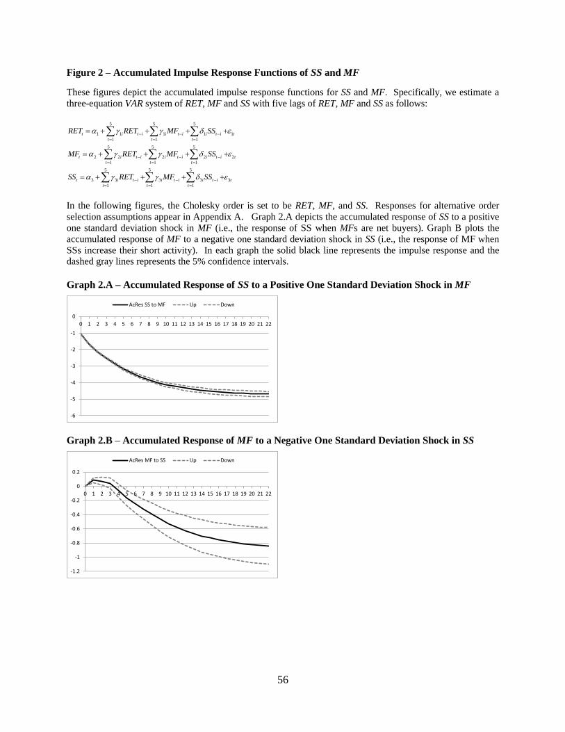
56

Figure 2 – Accumulated Impulse Response Functions of SS and MF

These figures depict the accumulated impulse response functions for SS and MF. Specifically, we estimate a

three-equation VAR system of RET, MF and SS with five lags of RET, MF and SS as follows:

5 5 5

1 1 1 1 1

1 1 1

5 5 5

2 2 2 2 2

1 1 1

5 5 5

3 3 3 3 3

1 1 1

t i t i i t i i t i t

t t t

t i t i i t i i t i t

t t t

t i t i i t i i t i t

t t t

RET RET MF SS

MF RET MF SS

SS RET MF SS

In the following figures, the Cholesky order is set to be RET, MF, and SS. Responses for alternative order

selection assumptions appear in Appendix A. Graph 2.A depicts the accumulated response of SS to a positive

one standard deviation shock in MF (i.e., the response of SS when MFs are net buyers). Graph B plots the

accumulated response of MF to a negative one standard deviation shock in SS (i.e., the response of MF when

SSs increase their short activity). In each graph the solid black line represents the impulse response and the

dashed gray lines represents the 5% confidence intervals.

Graph 2.A – Accumulated Response of SS to a Positive One Standard Deviation Shock in MF

Graph 2.B – Accumulated Response of MF to a Negative One Standard Deviation Shock in SS

-6

-5

-4

-3

-2

-1

0

0 1 2 3 4 5 6 7 8 9 10 11 12 13 14 15 16 17 18 19 20 21 22

AcRes SS to MF Up Down

-1.2

-1

-0.8

-0.6

-0.4

-0.2

0

0.2

0 1 2 3 4 5 6 7 8 9 10 11 12 13 14 15 16 17 18 19 20 21 22

AcRes MF to SS Up Down

57

Figure 3 – Cumulative Abnormal Return of AveSS and AveMF Single Sorted Portfolios

The figure depicts the DGTW (1997)-adjusted cumulative abnormal returns for single sorted equally-weighted

portfolios up to 63 days following daily portfolio formation. SS is the daily ratio of the stock’s shorting volume

to total trading volume multiplied by negative one (in %). MF is the daily ratio of net purchases by mutual

funds to total trading volume (in %). AveSS (AveMF) is the average of SS (MF) from t-5 to t-1. Specifically,

Graph 3.A (3.B) presents the portfolio returns of top and bottom AveSS (AveMF) decile portfolios presented in

Table 6 panel A (B). The sample period is January 3, 2005 to April 30, 2007, a total of 579 trading days.

Graph 3.A - Top and Bottom Deciles based on AveSS (t-5_t-1)

Graph 3.B - Top and Bottom Deciles based on AveMF (t-5_t-1)

-0.80%

-0.60%

-0.40%

-0.20%

0.00%

0.20%

0.40%

0.60%

0.80%

1.00%

1.20%

1 4 7 10 13 16 19 22 25 28 31 34 37 40 43 46 49 52 55 58 61

SS1 (Heavily shorted) SS10 (Lightly shorted)

-0.80%

-0.60%

-0.40%

-0.20%

0.00%

0.20%

0.40%

0.60%

0.80%

1.00%

1.20%

1 4 7 10 13 16 19 22 25 28 31 34 37 40 43 46 49 52 55 58 61

MF1 (Sell) MF10 (Buy)

58

Figure 4 – Cumulative Abnormal Return of Double Sorted Portfolios based on AveSS and AveMF

The figure depicts the average DGTW (1997)-adjusted cumulative returns for 63 trading days following daily

portfolio formation for double sorted equally-weighted portfolios. The graphed returns correspond to the

average returns of the portfolios reported in Specification 3 of Table 8. The portfolios are constructed based

on the intersection between AveSS and AveMF top and bottom quintiles. For example, the intersection between

MF1 and SS1 (denoted as MF1_SS1) is a portfolio of firms in the lowest AveMF (MF1) and the lowest AveSS

(SS1) quintiles. The sample period is January 3, 2005 to April 30, 2007, a total of 579 trading days.

-1.00%

-0.80%

-0.60%

-0.40%

-0.20%

0.00%

0.20%

0.40%

0.60%

0.80%

1.00%

1.20%

1 4 7 10 13 16 19 22 25 28 31 34 37 40 43 46 49 52 55 58 61

MF1_SS1 MF1_SS5 MF5_SS1 MF5_SS5DISAGREE

AGREE