Do Minimum Wage Increases reduce crime?the National Incident Based Reporting System (NIBRS), and the...

Do Minimum Wage Increases reduce crime?Zachary S. FoneDepartment of EconomicsUniversity of New Hampshire

Joseph J. SabiaProfessor of Economics, Director of Center for Health Economics & Policy StudiesSan Diego State University, University of New Hampshire & IZA

Resul CesurAssociate Professor of Healthcare EconomicsUniversity of Connecticut, NBER & IZA

March 2019

EPIONLINE.ORG

The Employment Policies Institute (EPI) is a non-profit research organization

dedicated to studying public policy issues surrounding employment growth.

In particular, EPI focuses on issues that affect entry-level employment.

Among other issues, EPI research has quantified the impact of new labor costs

on job creation, explored the connection between entry-level employment and

welfare reform, and analyzed the demographic distribution of mandated benefits.

EPI sponsors nonpartisan research which is conducted by independent economists

at major universities around the country.

This research was supported by a grant received from the Employment Policies

Institute. We also acknowledge support from the Center for Health Economics &

Policy Studies (CHEPS) at San Diego State University. The authors thank Melinda

Pitts, Dhaval Dave, Hope Corman, Tuan Nguyen, and participants at the 2018 Eastern

Economic Association meetings and the 2018 Southern Economic Association

meetings for useful comments and suggestions on earlier drafts of this paper. We

thank Thanh Tam Nguyen for outstanding research assistance.

EPIONLINE.ORG

Do Minimum Wage Increases reduce crime?

March 2019

Zachary S. FoneDepartment of EconomicsUniversity of New Hampshire

Joseph J. SabiaProfessor of Economics, Director of Center for Health Economics & Policy StudiesSan Diego State University, University of New Hampshire & IZA

Resul CesurAssociate Professor of Healthcare EconomicsUniversity of Connecticut, NBER & IZA

2 | EMPLOYMENT POLICIES INSTITUTE

EXECUTIVE SUMMARY Advocates have recently claimed that minimum wage increases may actually make our neighborhoods safer. By raising workers’ wages, the argument goes, legitimate labor market work will be more attractive to potential criminals and crime will fall. But what about those who lose their jobs? My new research, co-authored with Zachary Fone of the University of New Hampshire and Resul Cesur of the University of Connecticut, finds evidence that some affected younger workers turn to property crime, either due to excessive idleness or to replace their lost income. Higher minimum wages may, therefore, make some neighborhoods less safe. Our study examined two decades of data from the FBI’s Uniform Crime Reports, the National Incident-Based Reporting System, and the National Longitudinal Survey of Youth 1997. We focused on younger, less experienced teens and young adults who make up a disproportionate share of the minimum wage workforce, and who are more likely to face the brunt of any increase. We examined various types of crimes including property, violent, and drug crime, and used econometric strategies designed to isolate the effect of the minimum wage from macroeconomic conditions or other policies. This allowed us to be sure we were not confusing correlation with causation. Our results are clear. Over the period from 1998 to 2016, we find that minimum wage hikes increased property crime arrests among those ages 16 to 24. This is precisely the age group for whom we find minimum wage-induced job loss. Specifically, we find that a 10-percent increase in the minimum wage is associated with a 2-percent increase in property crime. We find no evidence of an increase in violent crime, which could be consistent with an income motive. Applying our estimates to the $15 minimum wage proposal now before Congress, we estimate that such a policy shock could lead to over 410,000 additional property crimes, generating $2.4 billion in additional crime costs to society. This conclusion stands in stark contrast to a report released by President Obama’s Council of Economic Advisers (CEA) in April 2016, which concluded that a minimum wage increase to $12 an

hour would have led to a 3-to-5 percent reduction in crime. While we respect the team of economists working at the CEA at that time, the report’s conclusion unfortunately rested on the assumption that minimum wage increases would only generate wage gains without any substantial offsetting employment or human capital effects. Our study shows that these effects cannot be ignored. The adverse employment effects generated by a $15 minimum wage are likely to increase property crime among some young adults. Fortunately, policymakers need not grapple with the tradeoff of higher wages for some at the expense of fewer jobs and more property crime among others. There are policy alternatives to the minimum wage that better help vulnerable workers and are far better targeted to those most in need. Expanding the Earned Income Tax Credit (EITC) has been shown to increase income and reduce poverty for many vulnerable workers without the unintended consequences of a higher minimum wage. Because workers have to earn income to receive the EITC, it has the added benefit of boosting employment. It is also far better targeted to the working poor than the minimum wage due to eligibility requirements. Expansions in the generosity and eligibility for the EITC would be far a more effective anti-poverty policy than raising the minimum wage. Raising the wages of low-skilled workers is a laudable policy goal. But if a government mandated raise comes at the expense of a job – and induces young jobseekers to earn money through illegal means — then policymakers should look elsewhere for better solutions to reduce poverty.

Dr. Joseph SabiaMarch 26th, 2019

SECTION 1:INTRODUCTION“Raising the federal minimum wage to $12 an hour could prevent as many as half a million crimes annually, according to a new report from the White House’s Council of Economic Advisers…as fewer people would be forced to turn to illegal activity to make ends meet.”

-Washington Post, April 25, 2016

Increasing incarceration and police can be effective (Levitt 2004; Corman and Mocan 2005; Chalfin and McCrary 2018), but expensive (Kearney et al. 2014) policy strategies to fight crime. Expenditures on police and the criminal justice system are estimated to be in excess of $286 billion per year (Bureau of Justice Statistics 2018).1 An alternative set of policies to deter crime, which are often less costly to taxpayers, includes those that improve labor market conditions and incentivize greater human capital acquisition. Among those at the margin of crime commission, criminal behavior is negatively related to employment opportunities (Mustard 2010; Schnepel 2017), wages (Gould et al. 2002, Yang 2017), and educational attainment (Machin and Meghir 2004; Anderson 2014). An April 2016 report from the White House Council of Economic Advisers (CEA) contrasted the high public costs of deterring crime via the criminal justice system with lower cost alternatives and recommended a novel policy strategy for combating crime: raising the minimum wage. The CEA argued that because minimum wage increases raise the hourly wages of low-skilled workers, the opportunity cost of engaging in criminal activity will rise, resulting in less crime. Using estimates of the crime elasticity with respect to wages from Gould et al. (2002), the CEA concluded that raising the Federal minimum wage from $7.25 to $12 per hour would decrease crime by 3 to 5 percent,

or 250,000 to 510,000 crimes annually (CEA 2016), resulting in $8 to $17 billion dollars per year in cost savings (CEA 2016). Consistent with the CEA’s prediction, recent work by Agan and Makowsky (2018) finds that minimum wage increases are negatively related to criminal recidivism. While intriguing, the CEA’s policy conclusion rests on the assumption that (i) minimum wage increases do not cause adverse labor demand effects that lead to more crime, or (ii) any adverse labor demand effects are sufficiently small to be swamped by wage gains (Agan and Makowsky 2018) or by enhanced expectations for higher-paying jobs. But there are important reasons to expect that the adverse labor demand effects from minimum wages may not always be small (Neumark 2017; Clemens and Wither 2016; Gittings and Schmutte 2016; Powell 2016; Baksaya and Rubenstein 2015; Totty 2015; Sabia et al. 2012; 2016). Minimum wage-induced job loss or hours reductions may lead to more property crime for economic reasons (Grogger 1998; Mustard 2010; Weatherburn and Schnepel 2015) and more violent crime for despair-related, emotionally expressive reasons (Wang et al. 2010; Nordin and Almen 2017).2 Minimum wage increases could also affect crime through their human capital effects, including impacts on school enrollment (Neumark and Wascher 2003; Pacheco and Cruickshank 2007) and on-the-job training (Neumark and Wascher 2001; Acemoglu and Pischke 2003). Additionally, they may also affect crime via their impacts on expected labor market opportunities, conditional on actual opportunities (Galbiati et al. 2017). The net effect of minimum wages on crime depends on (i) the magnitudes of wage, employment, schooling, and on-the-job training elasticities with respect to the minimum wage, (ii) the magnitudes of crime elasticities with respect to wages, employment, schooling, and on-the-job training, and (iii) the distribution of labor market effects of the minimum wage across individuals with heterogeneous propensities for crime, and (iv) on how higher minimum wages impact future expectations of labor market opportunities.

DO MINIMUM WAGE INCREASES REDUCE CRIME? | 3

1 The $286 billion estimate is comprised of $137 billion for police, $88 billion for corrections (e.g. prisons, jails, and staffing), and $62 billionfor the judicial system (Bureau of Justice Statistics 2018). Additionally, the FBI estimates that in 2016, the victims of property crime(excluding arson) suffered losses of $15.6 billion (FBI 2017c).

2 Wang et al. (2010) find that male ex-offenders in Florida released into counties with higher levels of unemployment are more likely to commit violent crime, which the authors suggest may be due to despair created by the lack of employment opportunities. They suggest this may also lead to male ex-offenders seeking alternative ways to express their masculinity (through violent crime, as opposed to employment). Nordin and Almen (2017) find that long-term unemployment spells are associated with increases in violent crime, which they suggest may be due to the strain created by these spells resulting in violent behavior.


The current study assesses the credibility of the CEA claim by comprehensively examining the relationship between minimum wages and crime. Using data from the Uniform Crime Reports (UCR), the National Incident Based Reporting System (NIBRS), and the National Longitudinal Study of Youth 1997 (NLSY97) from 1998 to 2016, our results provide little evidence of crime-reducing effects of the minimum wage. Instead, we find robust evidence that minimum wage hikes increase property crime arrests among teenagers and young adults ages 16-to-24, a population for whom minimum wages are likely to bind (Bureau of Labor Statistics 2016). We estimate a property crime elasticity with respect to the minimum wage of 0.2, an effect strongest in counties with populations greater than 100,000. This result is consistent with adverse labor demand effects of the minimum wage, a result that we confirm using data from Current Population Survey Outgoing Rotation Groups (CPS-ORG). We find little evidence that minimum wage increases affect violent or drug crimes, or net crime among older individuals, but do increase delinquency-related crimes related to teenage idleness (Jacob and Lefgren 2003; Luallen 2006; Anderson 2014). Moreover, in contrast to Agan and Makowsky (2018), we find no evidence that minimum wage increases reduced net crime among working-age individuals, suggesting that different margins of criminal behavior may be affected by minimum wages. A myriad of tests of the common trends assumption, including an event study analysis, support a causal interpretation of our estimates. Moreover, estimates of the effect of the minimum wage on “treated workers” in the NLSY97 add to our confidence in interpreting our findings causally. Our results show that minimum wages increase the probability of property crime commission among those bound by such hikes. To put our findings in the context of the 2016 CEA report, increasing the Federal minimum wage to $12 would represent a 66 percent increase in the current Federal minimum wage. Lower bound intent-to-treat (ITT) estimates from the UCR suggest that a $12 minimum wage would result in approximately 231,000 additional property crimes, generating

annual criminal externality costs of $1.3 billion (in 2018$) (McCollister et al. 2010). Moreover, the Raise the Wage Act of 2019 (HR 582) would raise the Federal minimum wage by 107 percent to $15 per hour.3 Our estimates suggest that this minimum wage hike would generate over 410,000 additional property crimes and $2.4 billion per year in additional crime costs. We conclude that increasing the minimum wage will at best be ineffective at deterring crime and at worst will have unintended consequences that increase property crime among young adults.

SECTION 2:BACKGROUND

Crime, the Labor Market, and Human Capital Becker’s theory of rational crime (1968) posits that criminal behavior is responsive to labor market conditions and human capital acquisition, and there is strong empirical evidence to support this theory. First, studies that have exploited changes in local employment conditions for populations on the margin of criminal behavior find that crime is positively related to unemployment rates (Raphael and Winter-Ebmer 2001; Gould et al. 2002; Machin and Meghir 2004; Levitt 2004; Oster and Agell 2007; Lin 2008; Mustard 2010) and business cycle contractions (Arvanites and Defina 2006; Rosenfeld and Fornango 2007). Recidivism also decreases when low-skilled job opportunities in construction and manufacturing rise (sectors more willing to hire ex-offenders) in the communities to which ex-offenders are released (Schnepel 2017). In addition, there is strong evidence that criminal behavior responds to wages. Gould et al. (2002) find that a 10 percent increase in the wages of non-college-educated men is associated with a 5.4 percent decrease in property crime and 10.8 percent decrease in violent crime.4 Along the same lines, Yang (2017) finds that ex-offenders released in counties with higher low-skilled wages are less likely to recidivate, particularly in sectors more willing to hire ex-offenders.

3 House Resolution (HR) 582 was introduced by Congressman Bobby Scott (D-VA) on January 16, 2019 and endorsed by House Speaker Nancy Pelosi (D-CA).

4 They also find that a one percentage point increase in the unemployment rate for non-college-educated working males ages 18 to 65 is associated with a 2.3 percent increase in property crime and a 1.3 percent increase in violent crime.

Second, increases in educational attainment may reduce crime. Raising the minimum legal school dropout age leads to a decline in criminal behavior among affected students (Lochner and Moretti 2004; Machin et al. 2011; Anderson 2014). These schooling effects can be explained by (i) incapacitation effects (Jacob and Lefgren 2003; Luallen 2006) as well as enhanced human capital acquisition (Lochner and Moretti 2004; Machin et al. 2011), the latter of which may change both the opportunity costs of crime as well as the tastes for crime.5 Crime-reducing effects of human capital acquisition can also be attained through on-the-job training (Lochner 2004), which is expected to increase workers’ wages (Mincer 1962; Brown 1989). On-the-job training has an important impact on the wages of young adult workers without a college degree (Lynch 1992).

Effect of Minimum Wages on Labor Market Outcomes

Minimum wages may affect each of the labor market outcomes described above, thereby impacting crime. First, there is strong and uncontroversial evidence that minimum wage increases raise the wages of low-skilled teenage and young adult workers (Card and Krueger 1994; Neumark and Wascher 2008; Dube et al. 2010; Allegretto et al. 2011; Sabia et al. 2012; Neumark et. al. 2014a,b; Jardim et al. 2018). Estimated wage elasticities from this literature are around 0.1 to 0.3.6 In contrast, the literature on the employment effects of minimum wages is far more controversial. Studies have taken a number of approaches to identify employment effects, including exploiting (i) variation over time and across jurisdictions in statutory minimum wages (Card and Krueger 1994; 1995; Burkhauser et al. 2000; Neumark and Wascher 2008; Dube et al. 2010; Allegretto et al. 2011; Sabia et al. 2012), (ii) heterogeneity in bindingness of the minimum wage across skill-levels in the population,

including individual wages (Stewart 2004; Thompson 2009; Sabia et al. 2012; 2016; Clemens and Wither 2016), or (iii) jurisdiction-level differences in bindingness of a Federal minimum wage change due to pre-treatment differences in minimum wage levels (Clemens and Wither 2016). Neumark and Wascher (2008) concludes that studies using the most credible identification strategies point to adverse employment effects for low-skilled workers, particularly teens, with elasticities in the range of -0.1 to -0.3.7

However, a number of recent studies have challenged the canonical consensus that minimum wages have adverse labor demand effects. Dube et al. (2010) compare employment elasticities obtained using contiguous county-pairs across state borders to those found when using canonical state-level panel models and conclude that the latter estimates are confounded by spatial heterogeneity.Their preferred border county approach suggests that the low-skilled employment effects of minimum wages are statistically indistinguishable from zero.8

Like Dube et al. (2010), Allegretto et al. (2011) contend that state-by-year panel studies that rely on two-way fixed effects models (see, for example, Sabia 2009) fail to disentangle the employment effects of minimum wages from spatial heterogeneity. They find that after controlling for state-specific linear time trends and census division-specific year effects, minimum wage increases have no effect on teen employment. Neumark et al. (2014a,b) challenge the conclusions of Dube et al. (2010) and Allegretto et al. (2011) by suggesting that (i) contiguous counties across state borders are often not the best treatment-counterfactual pairs, and (ii) controlling for state-specific linear time trends may generate variation in the minimum wage that is conflated with the state business cycle. Employing a synthetic control approach for each “treatment” county, Neumark et al. (2014a) find that positive weights are often assigned to non-border counties when generating a synthetic


5 Anderson (2014) finds little evidence of displacement effects of crime in schools.6 These estimated wage elasticities are “intent-to-treat” estimates that are often far less than one, often closer to 0.1 to 0.2. This is because

not all low-skilled workers earn wages such that they are affected by minimum wage increases and those that are may earn a wage between the old and new minimum wage.

7 There are exceptions to this elasticity range. Sabia et al. (2012) study the effects of a minimum wage increase on employment in New York from 2004-2006. They find that minimum wages adversely affect the employment of young, low-skilled workers, with an employment elasticity of -0.7. Additionally, Sabia et al. explicitly test the common time trends assumption, where they find that their estimates do not appear to be driven by pre-existing employment trends or endogenous minimum wage policy implementation.

8 However, it is important to note that many of these estimates are insufficiently precisely estimated to rule out estimates obtained from many canonical two-way fixed effects models using non-border counties as counterfactuals.

county with similar pre-treatment employment trends. Findings from a synthetic control approach generally confirm the canonical two-way fixed effects approach. Neumark et al. (2014b) also show that controlling for state-specific time trends of higher-order polynomials (e.g. third-order polynomials and higher) rather than linear time trends generates findings consistent with adverse labor demand effects (see also Neumark and Wascher 2017).9,10 A handful of studies have exploited heterogeneity across jurisdictions or workers in the bindingness of state or Federal minimum wages, generating identifying variation using (i) the pre-treatment share of low-skilled workers residing in the jurisdiction (Stewart 2004; Thompson 2009), (ii) the pre-treatment state minimum wage, which generates heterogeneous bindingness of a national minimum wage change (Clemens and Wither 2016), and (iii) the wage rate of a worker in the pre-treatment period (Clemens and Wither 2016), which affects whether the worker is directly affected by the minimum wage. Many of these studies (Thompson 2009; Clemens and Wither 2016), though not all (Stewart 2004), find evidence of negative employment effects of minimum wages. Finally, emerging experimental evidence, which overcomes the endogeneity of minimum wage policy via randomization, provides evidence consistent with adverse labor demand effects of the minimum wage for low-skilled workers. Horton (2018) conducts an experiment in which minimum wages are randomly assigned to firms that posted job openings online. He finds that a higher minimum wage raised the wages of employed workers, but also reduced hiring and hours worked among workers. Horton (2018) also discovers evidence of labor-labor substitution whereby less productive workers were adversely affected. While much of the minimum wage-employment literature has focused on short-run effects on employment levels, Meer and West (2016) argue that measuring employment growth rates may be more important to capture dynamic effects,

which traditional panel fixed effects models struggle to capture and state-specific linear time trends attenuate. When Meer and West (2016) allow for dynamic effects of minimum wages on employment growth, they find consistent evidence of adverse employment effects. Minimum Wages and Hours Worked. A number of studies have examined the hours effects of minimum wage increases to capture, in part, how minimum wages affect the intensive margin of work (Couch and Wittenburg 2001; Jardim et al. 2018; Sabia et al. 2018). In general, these studies find that minimum wage increases are associated with reductions along the intensive margin of employment for low-wage workers. For instance, Couch and Wittenberg (2001) draw data from the 1979-1992 CPS and find an elasticity of minimum wages to hours worked of around -0.5 for teenagers ages 16-to-19. Using more recent data from 1991 to 2013, Sabia et al. (2018) continue to find negative effects of minimum wage increases on hours worked (conditional on employment) among 16-to-20 year-olds. Local Minimum Wages and Living Wage Ordinances. While most studies have focused on the effects of state and Federal minimum wage changes, others have examined the effects of local minimum wages on labor market outcomes, with mixed results. Using administrative data and a synthetic control approach, Jardim et al. (2018) find that a large local minimum wage increase in Seattle (from $11 to $13 per hour) resulted in a 3.1 percent increase in wages of low-skilled workers, but a 9.4 percent decrease in hours worked and 6.8 percent decrease in employment.11 The authors concluded that hours reductions were so large that average earnings fell for low-skilled workers. In contrast, studies of local minimum wages in San Francisco (Schmitt and Rosnick 2011), Santa Fe (Schmitt and Rosnick 2011), and San Jose (Allegretto and Reich 2018) find evidence of minimum wage-induced wage gains, but no adverse employment effects; whereas, Luca and Luca (2017) find that the minimum wage increases in San Francisco were associated with


9 See also Allegretto et al. (2017).10 There is also evidence that the effects of minimum wages may differ across the business cycle (Addison et al. 2013; Sabia 2014).

Using CPS data from 1989-2012, Sabia finds that minimum wage increases reduce low-skilled employment more during recessions than expansions. During recessions, estimated employment elasticities can be as high as -0.3 to -0.5, and during expansions can range from 0 to -0.2. These findings are consistent with the hypothesis that employers are more likely to shed low-skilled workers during recessions when minimum wages rise.

11 Allegretto and Reich (2018) conclude that much of the local minimum wage increases in San Jose were absorbed by increases in restaurant prices.


12 Neumark and Adams (2003a) estimate the fraction of workers in the bottom quartile of the wage distribution that are potentially affected by living wage laws. This varies from 3 to 6 percent for laws that cover municipal employees, 15 to 20 percent for laws that cover contractors, and around 80 percent for laws that cover businesses who receive financial assistance. Neumark and Adams (2005a) suggest the larger bite of living wage laws which cover businesses who receive financial assistance may be explained by higher concentrations of living wage laws in contiguous or nearby labor markets for cities which also cover business assistance recipients.

13 A handful of studies have taken the case study approach to estimate the wage and employment effects of living wage ordinances (Brenner 2005; Fairris 2005; Reich et al. 2005). Studying the impact of a living wage ordinance that impacted workers at the San Francisco International Airport, Reich et al. (2005) find that the ordinance increased the wages of low-wage workers, with evidence of adverse employment effects. Similarly, Brenner (2005) finds that the living wage ordinance in Boston did not reduce employment or hours worked, yet this ordinance applied only to public contractors, where Neumark et al. (2012) also found evidence of smaller employment impacts. Finally, Fairris (2005) studies the effect of Los Angeles’ living wage ordinance, and finds that the law increased wages for low-wage workers, but also led to adverse employment effects, with an employment elasticity of roughly -0.1.

14 Warren and Hamrock (2010) find some modest evidence that larger minimum wage increases may have small negative effects on high school completion rates in states where students are permitted to drop out before age 17.15 Most studies in this small literature have used a difference-in-differences identification strategy that exploits variation in minimum wages

across jurisdictions and over time. There are exceptions to this approach. For instance, Hashimoto (1987) uses national data between 1947 and 1982 to estimate a time series regression and finds that Federal minimum wage increases are positively related to property crimes for youths ages 15-to-19, with estimated elasticities of 0.1 to 0.5.

restaurant closures. In addition to local minimum wages, over 100 localities in the U.S. have introduced living wage laws, intended to lift a low-wage full-time worker living in a family of average size out of poverty. Living wages differ from local minimum wages in that they are typically set higher than minimum wages and do not cover all forms of employment. Living wage ordinances generally cover municipal employees, public contract workers, workers in businesses who receive economic/financial assistance from the state or local government, or hotel workers. The types of workers covered can vary widely across localities with living wage laws.12 Nationwide studies of the labor market effects of living wages find that living wage ordinances raise the wages of low-wage workers, yet also lead to adverse employment effects (Neumark and Adams 2003a,b; Neumark and Adams 2005b). Neumark and Adams (2005a) find that ordinances which cover businesses who receive financial assistance from city governments for economic development generate larger wage increases and employment reductions than public contractor-only ordinances.13 Minimum Wages and Human Capital Acquisition. Raising the minimum wage may also affect crime via its effects on schooling and job training. Evidence on the schooling effects of minimum wages are somewhat mixed. Early studies find heterogeneity in schooling effects across income groups, reducing enrollment for teenagers in low-income families while increasing enrollment for those in high-income families (Ehrenberg and Marcus 1980; 1982). More recent studies find adverse school enrollment effects of minimum wages (Neumark and Wascher 2003; Pacheco and Cruickshank 2007)

and little impacts on overall school attainment (Card 1992; Campolieti et al. 2005; Warren and Hammock 2010; Sabia 2012).14 There is stronger evidence that minimum wages reduce on-the-job training (Neumark and Wascher 2001; Acemoglu and Pischke 2003), a finding consistent with the hypothesis that wage floors reduce an employer’s flexibility to finance job training out of workers’ wages (Rosen 1972).

Minimum Wages and Crime The literature on the crime effects of minimum waged is recent and small and was unmentioned in the April 2016 CEA report. Estimates obtained in this literature are sensitive to the (i) low-skilled population, (ii) time period, and (iii) margin of criminal behavior examined.15

Hansen and Machin (2002) examine the introduction of a new national minimum wage law in the United Kingdom and find that crime declines more in localities with larger shares of low-wage workers. Fernandez et al. (2014) use a clever identification strategy to estimate the effect of living wage ordinances enacted between 1990 and 2010 on overall crime rates for 239 large U.S. cities. They identify “control” cities as those that narrowly defeated living wage ordinances or passed such ordinances, but had them enjoined or repealed by state courts, and find that living wage increases are associated with reductions in both property and violent crimes. Although not emphasized in their paper, Fernandez et al. (2014) also find that minimum wage increases are associated with reductions in property and violent crimes, though these associations are sensitive to the inclusion of observable controls and city-specific time trends. In contrast, Beauchamp and Chan (2014) use individual-level panel data over

a comparable period, and focusing on low-wage workers for whom minimum wages were more likely to bind, find that minimum wage increases increase property and violent crimes among teenagers, but often find the opposite effect for young adults. Finally, a new working paper by Agan and Makowsky (2018) explores the impact of minimum wage increases on recidivism. They examine six million recently released prisoners across 43 states from 2000 to 2014 and find that minimum wage increases are associated with a decline in recidivism, primarily through reduced property and drug crime.16 The authors posit that wage gains from minimum wage increases dominate any negative employment effects. Their implied property and drug crime elasticities are quite large, ranging from -0.571 to -0.449, which would suggest that large shares of ex-offenders are bound by minimum wage increases.17

We contribute to this literature by using three large national datasets over a two-decade period to comprehensively examine the impact of Federal, state, and local minimum wages on crime. In contrast with many prior papers, our study (i) focuses on younger, lower-skilled individuals for whom minimum wages are most likely to bind (Lochner and Moretti 2004; FBI 2017a), (ii) explicitly examines employment, hours, and human capital effects of minimum wages over the same time period (and occasionally for the same people for whom) we measure crime, (iii) explores the sensitivity of our findings to tests of the common trends assumption, including event studies, distributed lag models, controls for jurisdiction-level time trends, and pseudo-falsification tests on demographic groups that should be less affected by minimum wages, and (iv) examines overall crime rates that include first-time arrests as well as criminal arrests that do not result in incarceration and release. Finally, we attempt to understand and

reconcile sometimes conflicting results across the existing small minimum wage-crime literature.

SECTION 3:DATA AND METHODS

Data The primary data source for our crime analysis is the Uniform Crime Reports (UCR), supplemented by data from the National Incident-Based Reporting System (NIBRS) and the National Longitudinal Survey of Youth 1997 (NLSY97). Each of these datasets has advantages and disadvantages, which we discuss below. From the UCR, we generate county-by-year criminal arrest rates from 1998 to 2016 by the age of the offender. Our primary “treatment group” is comprised of teenagers and young adults ages 16-to-24, an age cohort for whom minimum wages are most likely to bind (Bureau of Labor Statistics 2016). Arrest data are collected for property crimes (larceny, burglary, motor vehicle theft, and arson), violent crimes (homicide, rape, robbery, and aggravated assault), drug-related crimes (selling and possession), and other minor crimes often linked to idleness and delinquency (vandalism, liquor law violations, drunkenness, and disorderly conduct). To assure data quality, we drop county-year arrest rates that are greater than two standard deviations from the county arrest rate mean, control for the number of agencies that report to a county each year, and limit our sample to counties where at least 65 percent of agencies report arrest data (see, for example, Anderson 2014).18 Alternate methods of ensuring consistent reporting, including requiring

16 In addition, they find that expansions in the state Earned Income Tax Credit (EITC) reduces recidivism among women, consistent with the EITC increasing returns to legitimate employment. The authors posit that this result driven by eligibility rules that make the EITC bind most strongly for custodial parents.

17 Estimated intent to treat estimates of wage elasticities with respect to the minimum wage for low-wage workers tend to range from 0.1 to 0.2 (Card and Krueger 1994; Neumark and Wascher 2008; Dube et al. 2010; Allegretto et al. 2011; Sabia et al. 2012; Neumark et. al. 2014a,b; Jardim et al. 2018).

18 Explicitly, we utilize the “coverage indicator” sample criterion:

Where c denotes county, i denotes agency, and t denotes year. For a county where all agencies report 12 months of arrest data, the coverage indicator takes on the value of 100. For a county where none of the agencies report arrest data for any month, the coverage indicator takes on the value of zero. The coverage indicator measure was developed by the ICPSR (US DOJ 2017), and has been used by researchers as a sample criterion to assure data quality (see Freedman and Owens 2011; Thomas and Shihadeh 2013). Alternate cutoffs of the percentage of agencies reporting within the county (e.g. 60 percent, 75 percent, or 90 percent) generate a similar pattern of results.



19 Appendix Table 1B shows mean arrest rates for specific property, violent, and minor crimes in the UCR.20 These data also permit us to control for individual fixed effects to more effectively disentangle the effects of local minimum wages from

difficult-to-measure time-invariant individual characteristics and examine person-specific changes in minimum wages, employment, and crime. In supplemental analysis, we take this tack, though results are somewhat less precisely estimated.

21 Moreover, the NLSY97 ceased asking crime questions to all the respondents starting in round 8 of the survey (2004), asking crime questions only to individuals who had reported being arrested at least once beginning 2004 in addition to about 10 percent of survey participants as a control group.

a balanced panel of agencies, generated a similar pattern of results. Means of county-level arrests per 1,000 population are reported in Table 1. The average property crime arrest rate among 16-to-24 year-olds over the sample period is 15.83 per 1,000. For violent and drug arrests, the means are 5.04 and 16.40 per 1,000, respectively. As expected, arrest rates decline by age and are larger for men than women (see Appendix Table 1A).19

To supplement crime data from the UCR, we draw data from the NIBRS from 1998 through 2016. A key advantage of these data is that we can measure race/ethnicity-specific criminal incidents for 16-to-24 year-old arrestees, which is not possible with the UCR. This may be important if there are heterogeneous impacts of minimum wages by race or ethnicity. However, external validity using the NIBRS is limited. As of 2016, 38 states and the District of Columbia reported to the NIBRS (FBI 2017b), which represents 37.1 percent of the coverage in the UCR program and smaller, more rural jurisdictions, are overrepresented (FBI 2017a). Thus, if there are heterogeneous impacts of minimum wages by jurisdiction location and size, this could explain differences in results across the UCR and NIBRS. Means of agency-level incident counts from the NIBRS are shown in Appendix Table 1C. Finally, we add to the above analysis using individual-level panel data from the National Longitudinal Survey of Youth 1997 from 1998 through 2016. A key advantage of these longitudinal data is that we can identify low-wage workers who earn wages such that they are affected by future minimum wage increases. Thus, while the UCR- and

NIBRS-based analyses will permit us to identify intent-to-treat (ITT) estimates, the NLSY97 will permit estimates of the effect of treatment-on-the-treated (TOT). Moreover, the NLSY data permit us to measure crime that does not necessarily result in arrest, as well as jointly model labor market outcomes and criminal behavior.20 While Current Population Survey data permits us to examine net labor demand effects over the same period during which we measure crime, the NLSY97 actually permits us to examine crime and employment effects for the same persons. Despite these advantages, the NLSY97 data have a number of limitations. Data collected as part of the NLSY97 survey are self-reported and hence the crime variables are likely to understate the true prevalence of crime. However, as long as such measurement error is orthogonal to minimum wage changes, estimated policy impacts in terms of percent changes (relative to mean reporting crime) should be unbiased. Second, as the original sample consists of 8,983 respondents, the sample is not designed to be representative of low wage workers at the jurisdiction-by-year level.21 Often, there are very small numbers of low wage workers bound by minimum wage increases, which might suggest that estimates may be imprecise and sensitive to model specification. Thus, estimates obtained from the NLSY97 should be treated as suggestive as opposed to being conclusive. Our primary sample consists of approximately 38,000 person-years for individuals ages 16-to-24 for whom self-reported criminal engagement information is available. We generate five measures of crime using responses to seven questionnaire

22 The following are the survey questions used for the NLSY crime questions. For each survey question, the possible answers are “Yes” and “No.”

Property Crime Items:“Since the last interview on, have you stolen something from a store or something that did not belong to you worth less than 50 dollars?

“Since the last interview on, have you stolen something from a store, person or house, or something that did not belong to you worth 50 dollars or more including stealing a car?”

“Since the last interview on, have you purposely damaged or destroyed property that did not belong to you?”

“Since the last interview on [date of last interview], have you committed other property crimes such as fencing, receiving, possessing or selling stolen property, or cheated someone by selling them something that was worthless or worth much less than what you said it was?”

Violent Crime Item:“Since the last interview on, have you attacked someone with the idea of seriously hurting them or have had a situation end up in a serious fight or assault of some kind?”

Drug Crime Item:“Since the last interview on, have you sold or helped to sell marijuana (pot, grass), hashish (hash) or other hard drugs such as heroin, cocaine or LSD?”

Arrest Item:“Since the date of last interview on, have you been arrested by the police or taken into custody for an illegal or delinquent offense (do not include arrests for minor traffic violations)?”

23 Following Beauchamp and Chan (2014), we assume that the absence of response is because of inactivity. Thus, we replace missing values for crime variables to zero for those who ever reported criminal behavior. Estimates without replacing missing crime variable observations produce similar results to those presented here.

items.22 Any Crime is set equal to 1 if a survey participant reported committed a drug crime, a property crime (theft, damaging property, other property crime), or a violent crime (assault) since the date of the last interview, and is set equal to 0 otherwise; Property Crime is set equal to 1 for individuals who reported they had committed a theft or a property crime, or had damaged others’ property since the date of the last interview, and is set equal to 0 otherwise; Violent Crime is set equal to 1 for individuals who reported committing assault since the date of the last interview, and is set equal to 0 otherwise, Drug Crime is set equal to 1 for individuals who reported selling drugs and is set equal to 0 otherwise; and Arrest, set equal to 1 if respondents had been arrested and 0 otherwise.23 Appendix Table 2 shows means of these crime outcomes from the NLSY.

Minimum Wages and Living Wages Our main policy variable of interest for the UCR and NIBRS-based analysis is the higher of the Federal, state, or local minimum wage, MW. Federal and state-level minimum wages are collected from the United States Department of Labor, Wage and Hour Division. For county and city-level minimum wages, we use data compiled by Vaghul and Zipperer (2016) and update these data through 2016 via our own searches of local minimum wage ordinances.

In addition, we measure living wage ordinances using effective dates compiled from the National Employment Law Project (2011) as well as our own individual contacts with local governments. During the period from 1998 to 2016, there were 3 Federal minimum wage increases, 217 state minimum wage increases, 77 local minimum wage increases, and 116 living wage ordinances enacted. Figure 1 shows county-level variation in minimum wages over the period under study. The average state-legislated minimum wage hike over the 1998-2016 period was $0.55 (in 2016$) and 12 states indexed their minimum wages to a state-specific inflation rate. For the NLSY97-based analysis, our key treatment variable differs as we identify a treatment-on-the-treated (TOT) estimate. Following Currie and Fallick (1996), we define Binding MW as an indicator set equal to 1 if an individual is employed and earns a wage at year t that was no lower than the state or local minimum wage at year t and no higher than the state or local minimum wage at year t+1, and set equal to 0 if a worker earned a wage higher than the minimum wage at year t+1 or lower than the minimum wage at year t (i.e. because he or she was a tipped or informal worker not bound by the minimum wage). Thus, by construction, our estimation sample is limited to those who were employed in year t. Given that wage spillovers are possible to those who earn wages at year t higher than the


minimum wage at t+1 if firms engage in labor-labor substitution (or treat such laborers as complements), we experiment with dropping workers who earn hourly wages that are higher than, but are within $1 or $2 of the next period’s minimum wage. We also experiment with dropping sub-minimum wage workers (e.g. informal workers or tipped employees) from the analysis sample. The results were qualitatively similar to those presented below.24

Empirical Strategies First, using the UCR, we estimate a two-way fixed effects model of the following form via ordinary least squares (OLS):

(1) where Ycst is the criminal arrest rate per 1,000 population for those ages 16-to-24 in county c in state s in year t. Our main independent variable of interest ln(MW

cst), is the natural log of the maximum of the city,

county, state, or Federal minimum wage for a given county in year t, measured in the 2016 dollars.25

We also include a wide set of controls: Xcst

includes the number of agencies reporting arrests to a county, the share of the county population that is African American, Hispanic, and male, and the share of individuals in the state ages 25 and older with a Bachelor’s degree or higher; Cst is a vector of state-level crime policy controls, including shall issue concealed carry permit laws, the natural log of

law enforcement employees per 1,000 population, and the natural log of police expenditures per 1,000 population in 2016 dollars; Est is a vector of state-level economic controls, including the natural log of the prime-age (ages 25-to-54) average hourly wage rate in 2016 dollars and the natural log of the prime-age male unemployment rate; and Pst is a vector of state-level health and social welfare policies, including whether the state has a refundable EITC, whether the state Medicaid program has been expanded to include childless adults, whether all vehicles are exempt from an asset test for Supplemental Nutrition Assistance Program (SNAP) eligibility, whether the minimum legal high school dropout age exceeds 17, E-verify mandates, ban-the-box employment laws, marijuana liberalization laws (marijuana decriminalization or legalization laws and medical marijuana laws), and the natural log of beer taxes in 2016 dollars.26 In some specifications, we also include an indicator for the presence of living wage laws, following Fernandez et al. (2014). For our NIBRS-based analysis, we use agency-by-year incident data, and estimate a fixed effects Poisson model of the following form:

(2) where Yacst denotes the number of incidents in agency a in county c in state s during year t and εacst is a stochastic disturbance term. Exposure for each unit is represented by E

acst, which can be proxied by


24 Following Currie and Fallick (1996), we also experimented with MW Gap, set equal to 0 if a worker earned a wage higher than the minimum wage at year t+1, and equal to the difference between the minimum wage in period t+1 and the worker’s wage in period t when the worker’s wage is between the old and new minimum wages. Albeit less precise, the pattern of results is similar for regressions that replace Binding MW with MW Gap.

25 The minimum wage for county c in year t is coded as the higher of the Federal, state, or local minimum wage, averaged by the share of the year that the prevailing minimum wage level is in effect. For example, if the prevailing minimum wage in a county is $8 (determined by the state minimum wage), and a city within the county enacts a minimum wage higher than the prevailing wage in the county (say, $9). The county minimum wage is coded as the weighted average of the higher of the county/city minimum wage, where the weight depends on the share of the year the wage is in effect. So, if the county minimum wage is in effect for the entire year and the city minimum wage is in effect for half of the year, the minimum wage for the county would be coded as $8.50. We experiment with alternative coding of the minimum wage, including a weighted average of the prevailing county wage and the city wage, where the weight depends on the share of the year the wage is in effect and the share of the county population that the city represents as of the 2010 Census, and find similar patterns of results.

26 We compile the share of population ages 25 and older with a Bachelor’s degree, the prime-age (ages 25-to-54) average hourly wage and the prime-age male unemployment rate using the CPS Merged Outgoing Rotation Groups. Population data are collected from the Surveillance Epidemiology and End Results, U.S. Population Data (SEER). Specifically, we gather county-by-age population data, as well as the share of the county that is male, Hispanic and African American from the SEER. Police employment and expenditures are generated using data from the Bureau of Justice Statistics. Shall issue laws are updated using the sources available in Anderson and Sabia (Forthcoming). State EITC data are collected from the Tax Policy Center and E-verify data are collected from Churchill and Sabia (2018). Minimum legal dropout age data are collected through 2008 using Anderson (2014) and updated to 2016 from the National Center of Education Statistics. SNAP rules on vehicles are collected from U.S. Department of Agriculture, Food and Nutrition Service. Medicaid eligibility is compiled using various reports by the Henry J. Kaiser Family Foundation. Ban-the-box laws are updated from Doleac and Hansen (2017) using the National Employment Law Project (2017). Marijuana liberalization laws are updated using Sabia and Nguyen (Forthcoming). Beer taxes are collected from the Beer Institute. Population-weighted means and standard deviations of the main dependent and independent variables can be found in Table 1.

27 We define large changes as those in the top 25th percentile of increases of real minimum wages (9.0%), and moderate changes as those in the top 50th percentile of increases of real minimum wage (4.6%).

the estimated population served by the reporting agency. The variables on the right-hand-side of equation (2) are identical to equation (1) except that we employ agency fixed effects as opposed to county fixed effects. Identification of ß1 and γ1 comes from within-state, and occasionally within-county, variation in minimum wages. For our estimates to be interpreted causally, the common trends assumption must be satisfied. We take a number of tacks to address this concern. First, following Fuest et al. (2018) and Simon (2016), we estimate an event study, taking into account that each jurisdiction may include multiple events:

(3) where Dcst is a set of indicators set equal to 1 if there was an event occurred j periods from period t. Our events are defined as (i) any real minimum wage increase, (ii) real minimum wage increases in the top 50th percentile of minimum wage increases, and (iii) real minimum wage increases in the top 25th percentile of minimum wage increases.27 Examining crime trends prior to minimum wage increases will allow us to test for common pre-treatment trends between “treated” and “control” jurisdictions. As an additional test of the common trends assumption, we estimate a distributed lag model which allows us to exploit the full distribution of magnitudes of minimum wage increases:

(4). Our independent variable of interest in equation (4) is the set of the one-year difference in the minimum wage hikes that happened j periods away. We prefer the leads and lags of minimum wage changes as opposed to minimum wage levels, as there are numerous overlapping minimum wages in our sample. Third, we examine the robustness of estimates of ß1 and γ1 in equations (1) and (2) to controls for state-specific time trends. The inclusion of controls for state-specific time trends is intended to mitigate

bias in the estimates of minimum wage effects. However, the inclusion of these trends, particularly linear state time trends, may come at a cost of reduced precision or, worse, conflating remaining minimum wage variation with jurisdiction-specific business cycles (Neumark et al 2014a,b; Neumark and Wascher 2017). Thus, we also examine the robustness of estimated crime elasticities to the inclusion of state-specific higher-order polynomial trends. Fourth, we explore heterogeneity in the impact of minimum wages across the age distribution. Older, more experienced individuals, may be less likely to be bound by the minimum wage or, may serve as labor-labor substitutes (or complements) for younger, less experienced workers. Thus, to ensure that any “post-treatment” trends we observe for 16-to-24 year-olds are not driven by differential trends unrelated to the minimum wage, we explore whether effects differ for older workers. While these are imperfect placebo tests, we expect smaller spillover effects to these workers. Finally, our use of the NLSY97 will permit us to examine minimum wage effects for those for whom minimum wages bind. Specifically, we estimate:

(5) where Yaist is an indicator for the type of crime we are observing for respondent i, in age group a (ages 16-to-24 vs. 25 and older), in state s, during year t. Our primary coefficient of interest, ß1, captures the effect of minimum wage increases on criminal behavior for respondents (in age group a) who are bound by such increases compared to those who are not. The vector Xist includes individual-level controls for race/ethnicity, age, math PIAT (Peabody Individual Achievement Test) scores, maternal education, and family income. The remainder of controls are identical to those in equations (1) and (2). Here, identification comes from changes in workers’ wages and/or changes in minimum wage policies that affect the bindingness of the minimum wage for a teen or young adult worker.

a


j


28 Estimates on the control variables present in Table 2 (column 4) appear in Appendix Table 3.29 In Table 3A, columns (1), (4), (7) we show results using only contemporaneous changes in minimum wages on the right-hand side of

the regression; columns (2), (5), and (8) does the same, but is restricted to the sample used to estimate the full set of lead and lagged effects of the minimum wage, and columns (3), (6), and (9) show the full distributed lag model described in equation (4).

30 For models that estimate crime effects for individuals ages 25 and older, we do not control for prime-age male unemployment rates, prime-age wage rates, or the share of individuals ages 25 and older with a college degree, as these measures may capture mechanisms through which minimum wages affect crime. Instead, following Clemens and Wither (2016) and Agan and Makowsky (2018), we control for the state-level housing price index (available from: https://www.fhfa.gov/DataTools/Downloads/Pages/House-Price-Index.aspx). This approach is designed to control for macroeconomic conditions that are not directly affected by minimum wage changes.

SECTION 4:RESULTS

UCR Findings Tables 2 through 7 show estimates ofβß1 from the UCR. All models are weighted by the county population and standard errors are clustered on the state (Bertrand et al. 2004). In Table 2, we present estimates of ß1 from equation (1).28 Column (1) presents findings from the most parsimonious specification, including only socio-demographic controls, while column (2) adds crime policy controls, column (3) adds economic controls, and column (4) adds social welfare and health policy controls. Across specifications in Panel I, we find consistent evidence that minimum wage increases are associated with increases in property crime arrests for 16-to-24 year olds. The estimated elasticity is remarkably stable across specifications, ranging from 0.210 to 0.261. These results suggest that minimum wage increases induce income-generating crimes among young adults, perhaps due to adverse labor demand effects. We find no evidence that minimum wage increases affect violent crime arrests (Panel II). For drug arrests (Panel III), estimated minimum wage elasticities are positive, ranging from 0.040 to 0.174, but are not statistically distinguishable from zero at conventional levels. To explore whether the effects we observe in Panel I of Table 2 can be explained by pre-treatment trends in property crime arrests, we next report results from the event study analysis described in equation (3). This approach also allows for heterogeneous treatment effects by the size of the minimum wage increase. In the main, Figure 2 shows that pre-treatment property crime arrest trends among 16-to-24 year-olds were similar for “treatment” and “control” counties. Following enactment of the largest minimum wage increases (top 25th

percentile), we see substantial increases in property crime. This pattern of pre- and post-treatment trends is consistent with minimum wage-induced increases in property crime. For smaller minimum wage increases, post-treatment trends show little effect of minimum wages on property crime. We find little evidence that minimum wages impact violent crimes (Figure 3), but do find longer-run increases in drug crime arrests associated with larger minimum wage increases (Figure 4). As an additional test of the common trends assumption, we estimate the distributed lag model outlined in equation (4) in Table 3A.29 Across property, violent, and drug crimes, we find little evidence of differential pre-treatment trends in crime. For property crime, we find evidence that crime increases after the adoption of minimum wage increases, consistent with the event study shown in Figure 2. Could the increases in property crimes for teens and young adults be explained by differential post-treatment trends unrelated to minimum wages? In Table 3B, we examine the sensitivity of crime effects to controls for state-specific linear and higher-order polynomial trends, following prior work in the minimum wage-employment literature (Allegretto et al. 2011; Neumark et al. 2014a,b). Reassuringly, findings in Panel I of Table 3B suggest that the impact of minimum wages are very robust to the inclusion of state-specific time trends. We consistently estimate property crime elasticities between 0.208 and 0.330. For violent (Panel II) and drug crimes (Panel III), there continues to be little evidence of minimum wage increase impacts. As a further test of the common trends assumption, we explore whether there are heterogeneous crime effects of minimum wage hikes across the age distribution.30 Older, more experienced individuals are less likely to be bound by minimum wages and hence any crime effects should likely be smaller. On the other hand, older individuals on the margin of crime commission may be more likely than the average older individual to be bound.

The results in Table 4 show that minimum wage hikes increase property crime arrests among teenagers ages 16-to-19 (Panel I, column 1) and young adults ages 20-to-24 (Panel I, column 2), with estimated elasticities of 0.162 to 0.270. There is little evidence of minimum wage-induced increases in property crime effects for those ages 25 and older, which adds to our confidence that estimates of ß1 for those ages 16-to-24 are not capturing differential jurisdiction-level time trends. For those ages 45-to-54, we detect some evidence of crime-reducing effects of the minimum wage (Panel I, column 6), consistent with what could be labor-labor substitution toward older workers. However, in contrast to those ages 16-to-24, the reduction in crime for 45-to-54 year-olds are sensitive to state-specific quadratic (Panel II) and fourth-order polynomial (Panel III) time trends. We find no evidence that minimum wages affect violent or drug arrests among older individuals (see Appendix Table 4).31

Finally, in column (8) of Table 4 and column (8) of Appendix Table 4, we present estimates of the effect of minimum wages on net crime among all working age individuals ages 16-to-64. The point estimates are uniformly positive and, with one exception, are statistically indistinguishable from zero. Estimated elasticities range for property crime range from 0.084 to 0.166.32

We next explore whether these effects differ by gender (Table 5), type of property crime (Table 6), and type of minimum wage ordinance (Table

7). With regard to gender, we find that both male and female property crime rise similarly in response to minimum wage increases, with estimated elasticities of 0.214 to 0.236 (Panel I, Table 5). Given that larcenies comprise 72 percent of all property crimes for 16-to-24 year-olds during our sample period, we unsurprisingly find that the increase in property crimes for teens and young adults is driven by larcenies (Panel I, Table 6), where the estimated minimum wage and crime elasticity is 0.241. There is no evidence that minimum wages affect other types of property (burglary, motor vehicle theft, and arson) or violent (homicide, robbery, rape, and aggravated assault) crimes. In Panel III of Table 6, we estimate the effect of minimum wage increases on more minor types of criminal arrests, including for vandalism, liquor law violations, drunkenness, and disorderly conduct. We find that minimum wage hikes increase disorderly conduct arrests, consistent with job-loss induced idleness among teens and young adults (Jacob and Lefgren 2003; Luallen 2006; Anderson 2014). To gauge whether crime effects differ across minimum wages as compared to living wage laws, in Table 7 we include an indicator for living wage laws in our model, as well as an interaction term for whether a living wage law applies to employers who receive financial assistance from the state or local government. For the financial assistance living wage provision, we find that laws including them are associated with a statistically


31 Following Clemens and Wither (2016) as well as Agan and Makowsky (2018), we experiment with a somewhat different identification strategy, where we exploit heterogeneous bindingness in Federal minimum wage changes by pre-treatment state minimum wage levels. Specifically, we define an indicator variable Bound, that is set equal to one for a state-year in which a state experiences a minimum wage increase that is due to one of the Federal minimum wage increases between 2007-2009, and zero otherwise. We then re-estimate equation (1), including the Bound indicator and the Ln(MW)*Bound interaction term (as well as the minimum wage main effect). In Appendix Table 5, we present these estimates for 16-to-24 year-olds. The coefficient estimate on the interaction term is not statistically distinguishable from zero at conventional levels.

32 Taken at face value (without regard to the statistical significance of estimates), estimates for property and violent crime suggest that the annual criminal externality costs generated over our sample period by all working age individuals from a 10 percent increase in the minimum wage was approximately $2.7 billion ($400 million for property and $2.3 billion for violent crime). To generate this cost estimate, we first gather part I property and violent crimes committed over the 1998-2016 period using the FBI’s Crime in the United States reports (available from: https://ucr.fbi.gov/crime-in-the-u.s/2016/crime-in-the-u.s.-2016/topic-pages/tables/table-1). We then use the UCR’s Arrests by Age, Sex, and Race files from 1998-2016 to calculate the share of property and violent crimes committed by 16-to-64 year-olds. To generate an estimate of the number of crimes committed by 16-to-64 year-olds, we calculate the product of the average crime counts over the 1998-2016 period from the FBI’s Crime in the United States report and the share of crimes committed by 16-to-64 year-olds from the UCR’s Arrests by Age, Sex, and Race files. Using our estimated crime elasticities with respect to the minimum wage of 0.084 for property crime (Table 4, column 8) and 0.081 for violent crime (Appendix Table 4, column 8), we estimate 69,746 additional property crimes and 9,993 additional violent crimes would be generated by a 10 percent increase in the minimum wage. Then, we use the per crime cost of a property offense of $5,739 (in 2018USD) and the per crime cost of a violent offense of $233,932 (in 2018USD) from McCollister et al. (2010) to estimate the total additional crime cost from a 10 percent increase in the minimum wage. We obtain an estimate of $2.7 billion, $400 million for property crime and $2.3 billion for violent crime.


33 An event study analysis in Appendix Figure 2 suggests that this increase in property crime for 16-to-24 year-olds may not be driven by differential pre-trends in property crime. Event study analyses available upon request show little evidence of differential pre-treatment trends in violent crime for our living wage ordinance measure.

34 In a study of coverage and representativeness of NIBRS data through 2013, McCormack et al. (2017) find that the NIBRS underrepresents more populous jurisdictions. They find that in the NIBRS data, there is no coverage in nine of the 20 most populous states in the U.S., and there is 25 percent coverage or less within the remaining 11 states. Furthermore, as of 2013, the NIBRS had not been implemented in 17 of the 25 most populous cities in the U.S., where NIBRS coverage begins at the 15th ranked city (Columbus, OH) in terms of population.

35 In Appendix Table 6, we present NIBRS estimates for all arrestees across various age groups (similar to Table 5) and continue to find little evidence of minimum wage increases influencing crime.

36 Means of labor market outcomes and school enrollment used in the CPS are available in Appendix Table 7.37 Given the log-log specification in Panels I and IV, we can interpret the coefficient estimates as elasticities.

significant 9.1 percent increase in property crimes. This result is consistent with evidence from the living wage-employment literature, which finds that living wage laws covering financial assistance recipients generates stronger adverse employment effects (Neumark and Adams 2005a).33 We also find some evidence that living wage ordinances are associated with increases in violent crime.

NIBRS Results In Table 8, we turn to the NIBRS to examine whether there are heterogeneous impacts of minimum wages on 16-to-24 year-olds by race/ethnicity. Within each panel of this table, we present estimates for all arrestees (column 1), non-Hispanic white arrestees (column 2), non-white arrestees (column 3), African American arrestees (column 4), and Hispanic arrestees (column 5) separately. Interestingly, across all race/ethnicity groups, we find little evidence that minimum wage increases affect any type of crime, including property crime. Crime effects tend to be more positive for non-whites, but none are statistically distinguishable from zero with estimated property crime elasticities range from 0.022 to 0.075. Because the UCR and NIBRS generate such different results on the impact of minimum wage increases on property crime arrests among 16-to-24 year-olds, in Table 9, we explore whether this difference in findings could be due to (i) geographic differences in UCR and NIBRS coverage, and (ii) differences in jurisdiction size. In column (1) of Table 9, we restrict our UCR sample to counties that are present in the NIBRS analysis sample. We still find a positive property crime effect, but the estimated elasticity is approximately 50 percent smaller than in the full UCR sample (0.115 versus 0.210), and the estimated effect is statistically indistinguishable from zero. This suggests some degree of heterogeneityin minimum wage effects by jurisdiction.

In the remaining columns, we explore heterogeneity in minimum wage effects by size of counties sampled in the UCR: those with populations of 100,000 or greater (column 2), those with populations between 25,000 and 100,000 (column 3), and those with than 25,000 residents (column 4). We find that the property crime effect is concentrated among large counties with populations of 100,000 or more, where we estimate an elasticity of 0.240. While remaining positive, the property crime effect becomes smaller in magnitude and less precise as we move from mid-to-small sized counties. Because our property crime effect in the UCR is concentrated among large counties, it is not surprising that estimated property crime elasticities from the NIBRS are smaller given that smaller, rural jurisdictions are overrepresented in the NIBRS.34,35

CPS Results An important mechanism for minimum wage increases to influence property crime is through their effects on the labor market outcomes of low-skilled workers. To explore this possibility, we draw data from the 1998-2016 Current Population Survey Outgoing Rotation Groups. We estimate the impact of minimum wage increases on the wages and employment of 16-to-24 year-olds from 1998-2016. We restrict our sample to individuals ages 16-to-24 with less than a high school diploma, as they are more likely to be bound by minimum wages and be on the margins of crime commission.36

Consistent with the prior literature, we find that minimum wage increases increase the hourly wages of teen and young adult workers, with estimated wage elasticities of 0.176 to 0.184 (Table 10, Panel I).37 However, we also find evidence that minimum wage increases lead to a reduction in low-skilled employment, with estimated employment elasticities of -0.147 to -0.217 (Panel II), and a reduction in usual weekly hours worked, with

estimated elasticities of -0.204 to -0.273 (Panel III), consistent with a wide body of literature (Neumark and Wascher 2008; 2017). These estimated employment and hours elasticities are remarkably similar to the property crime elasticities shown in Table 2 and are consistent with the hypothesis that adverse labor demand effects of minimum wage increases are an important mechanism for increases in property crime. Estimated effects of minimum wages on usual weekly hours (Panel IV) and usual weekly earnings (Panel V) are generally negative, although smaller and less precisely estimated. We find little evidence of school enrollment effects of the minimum wage (Panels VI and VII), suggesting that this human capital channel is relatively unimportant in explaining minimum wage-induced increases in property crime.38

NLSY97 Results In Table 11, we turn to the NLSY97 to examine TOT estimates for those for whom the minimum wage is binding, following an approach similar to Currie and Fallick (1996) and Beauchamp and Chan (2014). We find that 16-to-24 year-olds bound by the minimum wage are 1.8 percentage-points (12.9 percent) more likely to engage in criminal activity, driven by a 1.7 percentage-point (21.3 percent) increase in property crime. For minimum wage bound individuals ages 25 and older, we also find evidence of minimum wage-induced increases in property crime, as well as an increase in the probability of being arrested. Thus, we find no evidence to support the claim that minimum wage increases reduce crime among those who are directly affected by it.39 As our CPS-based estimates suggest, the lack of any crime-reducing effects of minimum wages may be explained by adverse labor demand effects borne by individuals bound by them. Our findings in Table 12 provide strong evidence that minimum wage increases negatively affect both the intensive and extensive margins of work, the likely mechanism at work. Our results show stronger property crime effects for those below the

median annual hours worked (Table 13, Panel I) as compared to individuals above the median (Table 13, Panel II), consistent with labor demand effects being an important mechanism at work.

Comparisons with Prior Estimates Two relatively recent papers produce some evidence of crime reducing effects of minimum wages. We attempt to explain differences in our results from this prior work. First, while focusing largely on living wages, estimates shown in Table 3A of Fernandez et al. (2014; p. 488) show that minimum wages enacted between 1990 and 2010 reduced overall property and violent crime in large cities. First, to replicate their specification, we generate total arrest rates per 100,000 population for the 239 largest cities (as of 1990) from the UCR, collect data on their controls, and use their preferred log-log specification to estimate the effect of minimum wage increases on overall property (Panel I) and violent (Panel II) crime arrests from 1990-2010.40 The results in column (1) of Table 14 are consistent with their results: minimum wage increases enacted between 1990 and 2010 resulted in large, statistically significant reductions in property and violent crimes. The inclusion of a set of observable demographic and macroeconomic controls used by Fernandez et al. (2014) (column 2) produces an elasticity of -0.094 for property crime and -0.237 for violent crime, though both estimates are statistically indistinguishable from zero at conventional levels. In columns (3) through (5), we include controls for city-specific time trends; in these specifications, estimated property crime elasticities become small and positive and violent crime elasticities fall to near zero. In Figure 5, we provide evidence on why the crime elasticities are sensitive to city-specific time trends. When we conduct an event study analysis using the specification outlined in column (1) of Table 14 (see left-hand-side of Figure 5), we find that between 1990 and 2010, property and violent crime arrests were trending downward prior to the enactment of minimum wage increases, a trend most pronounced

38 Using data from the CPS’s October Supplement from 1998-2016, we estimate the effects of minimum wage increases on school enrollment via probit (Panel VI) as well as using a multinomial logit model (Panel VII), following Neumark and Wascher (1995).

39 In Appendix Table 8, we present estimates from equation (5) that include individual fixed effects, which require individual-specific changes in the bindingness of minimum wages over time for identification. These estimates also show no evidence of declines in property crime. Estimates are positive and statistically indistinguishable from zero.

40 Following Fernandez et al. (2014), we gather data for this replication using https://www.ucrdatatool.gov/, where the FBI uses an imputation procedure to estimate crime rates for agencies with poor reporting. These data are only available through 2014.



41 As Appendix Figure 1 shows, much of the minimum wage variation during that period came from Federal minimum wage changes in states that were fully bound by the increase, including many states in the South and Midwest regions. These states were, it seems, already experiencing crime declines prior to the Federal minimum wage change.

42 In Appendix Table 9, we examine the 1998-2014 period to further explore whether the differences in our findings as compared to Fernandez et al. (2014) can be explained by the time period examined. We exclude data from 2015 and 2016 because imputed crime data used by Fernandez et al. (2014) are only available through 2014. Here, we find little evidence that minimum wages affect aggregate crime rates in the largest cities, where most estimated elasticities for property crime are positive, while for violent crime are mostly negative, yet small and close to zero. Moreover, event study analyses, available upon request, show little evidence of differential pre-treatment trends.

43 In the sample of arrestees of all ages, we use imputed UCR crime compiled by the ICPSR. These data include imputed crime counts for jurisdictions which have poor reporting, and are available from:

https://www.ojjdp.gov/OJSTATBB/ezaucr/asp/methods.asp44 We identify the state-years available in the National Corrections Reporting Program (NCRP) public use files by state and year of release

from prison, approximating the analysis sample used by Agan and Makowsky (2018). Additionally, we drop California from the analysis sample, as does Agan and Makowsky (2018). The NCRP public use files may be obtained from: https://www.icpsr.umich.edu/icpsrweb/NACJD/studies/37021

45 In Appendix Table 10, we present estimates using the Agan and Makowsky (2018) specification for 16-to-24 year-olds over the 2000-2014 and 2000-2016 period, which are consistent with our main results from Table 2.

among larger state minimum wage increases enacted between 1990 and 1997 (see Figure 6).41 On the right-hand-side of Figure 5, we show that this differential pre-trend disappears, as does the post-treatment decline in crime, when controls for city-specific linear time trends are included as controls.42 Second, Agan and Makowsky (2018) find that minimum wage increases enacted between 2000 and 2014 are associated with a reduction in recidivism rates, mainly through reduced property and drug crime. We explore whether our findings may differ due to (i) differences in the states and years comprising the analysis sample, (ii) demographic composition of arrestees, and (iii) margin of criminal behavior examined (recidivism versus overall crime). We collect data on the controls used by Agan and Makowsky (2018) to rule out observable controls as an explanation for differences in results. In column (1) of Table 15, we estimate the effect of minimum wage increases on total arrests using the UCR imputed crime data file, while limiting our sample to the states and years that were available in the National Corrections Reporting Program (NCRP), the data source used by Agan and Makowsky (2018).43,44 We also use a specification similar to that employed by these authors and include their control variables. Our results show no evidence that minimum wage increases affected net property or violent crime. Estimated elasticities with respect to the minimum wage are 0.155 for property crime, 0.090 for violent crime, and -0.137 for drug crime arrests, each statistically indistinguishable from zero at conventional levels. These estimated effects are far more positive than the implied recidivism elasticities

obtained by Agan and Makowsky (2018), -0.571, -0.141, and -0.449, respectively. Adding the full set of states and years available in the UCR from 2000-2014 (column 2), we continue to find no evidence of minimum wage-induced declines in net crime. To gauge whether results may differ across demographic groups, we also examine adults ages 18 and older (columns 3-4), adult males (columns 5-6), African American adults (columns 7-8). Across each of these demographic groups, we find no evidence of crime-reducing effects of minimum wages over the 2000-2014 period. Expanding the sample period through 2015 and 2016 (columns 4, 6, and 8) produces a similar pattern of results.45 Together with the findings of Agan and Makowsky (2018), our results in Table 15 suggest that minimum wage increases may have heterogeneous effects on different margins of criminal behavior, including first-time arrests as well as arrests that do not result in incarceration and release.

SECTION 5: CONCLUSION An April 2016 report from the White House Council of Economic Advisers claimed that raising the Federal minimum wage from $7.25 to $12 per hour could reduce crime by 3 to 5 percent, generating substantial social benefits. However, this conclusion rested on the assumption that minimum wage increases would only generate wage gains

with no offsetting employment or human capital effects. This study comprehensively examines the effects of recent changes to Federal, state, and local minimum wages on crime. Our results suggest that minimum wage increases enacted from 1998 to 2016 led to increases in property crime for those between the ages of 16-to-24, with an estimated elasticity of 0.2. This finding is robust to the inclusion of controls for state-specific time trends, survive falsification tests on policy leads, and persist for workers who earn wages such that minimum wage changes bind. Increases in property crime appear to be driven by adverse employment and hours effects of minimum wages. We find little evidence that minimum wage increases affect violent or drug crimes. The magnitude of our estimates suggests that a 10 percent increase in the minimum wage between 1998 and 2016 led to nearly 80,000 additional property crimes committed by 16-to-24 year-olds, generating annual crime costs of $459 million (2018$) (McCollister et al. 2010).46 Moreover, if our estimated crime elasticities are used to make predictions of future policy changes, raising the Federal minimum wage to $15 per hour, as the Raise the Wage Act of 2019 proposes, would generate approximately 410,000 additional property crimes and $2.4 billion in additional crime costs.47 These could be lower bound estimates if living wage ordinances also have the unintended consequence of increasing crime or if there are modest increases in delinquency-related crimes. Together, the findings from this study suggest that, in contrast to the CEA claim, higher minimum wages are unlikely to be an effective tool to fight net crime.


46 This estimate is obtained analogously to the procedure described in footnote 32. However, we focus on 16-to-24 year-olds as compared to 16-to-64 year-olds and use only the statistically significant elasticity we obtain for property crime among 16-to-24 year-olds (column 4 of Table 2) to estimate crime costs.

47 To generate this cost estimate, we first gather state part I property committed in 2016 using the FBI’s Crime in the United States report (available from: https://ucr.fbi.gov/crime-in-the-u.s/2016/crime-in-the-u.s.-2016/topic-pages/tables/table-3). We then use the UCR’s Arrests by Age, Sex, and Race files from 2016 to calculate the state-specific share of property crime committed by 16-to-24 year-olds. To generate the state-specific estimate of the number of crimes committed by 16-to-24 year-olds, we calculate the product of state-level crime counts from FBI’s Crime in the United States 2016 report and the share of crimes committed by 16-to-24 year-olds from the UCR’s Arrests by Age, Sex, and Race files. Then, to calculate the state-specific percentage change in the minimum wage caused by a $15 Federal minimum wage, we use the higher of the state or Federal minimum wage in July 2018 to calculate a state-specific measure of the increase in the minimum wage they would experience from a $15 minimum wage. Using our estimated property crime elasticity with respect to the minimum wage of 0.210 from column (4) of Table 2, we estimate the number of additional property crimes that would be generated in each state. Summing across states, we estimate 410,030 additional property crimes would be generated by a $15 minimum wage. Then, we use the per crime cost of a property offense of $5,739 (in 2018USD) from McCollister et al. (2010) to estimate the total additional crime cost from a $15 minimum wage of $2.4 billion.


REFERENCESAcemoglu, Daron, and Jorn-Steffen Pischke. 2003. “Minimum Wages and On-the-Job Training.” Research in Labor Economics, 22: 159-202.

Addison, John T.; Blackburn, McKinley L., and Chad D. Cotti. 2013. “Minimum wage increases in a recessionary environment.” Labour Economics, 23: 30-39.

Agan, Amanda Y, and Michael D. Makowsky. 2018. “The Minimum Wage, EITC, and Criminal Recidivism.” National Bureau of Economic Research, Working Paper 25116. 1-56. Available at: http://www.nber.org/papers/w25116

Allegretto, Sylvia A; Dube, Arindajit; Reich, Michael, and Ben Zipperer. 2017. “Credible Research Designs for Minimum Wage Studies: A Response to Neumark, Salas, and Wascher.” Industrial and Labor Relations Review, 70(3): 559-592.

Allegretto, Sylvia A.; Dube, Arindrajit, and Michael Reich. 2011. “Do Minimum Wages Really Reduce Teen Employment? Accounting for Heterogeneity and Selectivity in State Panel Data.” Industrial Relations, 50(2): 205-240.

Allegretto, Sylvia A., and Michael Reich. 2018. “Are Local Minimum Wages Absorbed by Price Increases? Estimates from Internet-Based Restaurant Menus.” Industrial and Labor Relations Review, 71(1): 35-63.

Anderson, D. Mark and Joseph J. Sabia. Forthcoming. “Child Access Prevention Laws, Youth Gun Carrying, and School Violence,” Journal of Law and Economics.

Anderson, D. Mark. 2014. “In school and out of trouble? The minimum dropout age and juvenile crime.” The Review of Economics and Statistics, 96(2): 318-331.

Arvanites, Thomas M., and Robert H. Defina. 2006. “Business Cycles and Street Crime.” Criminology, 44(1): 139-164.

Baskaya, Yusuf Soner, and Yona Rubinstein. 2015. “Using Federal Minimum Wages to Identify the Impact of Minimum Wages on Employment and Earnings across U.S. States.” Unpublished paper.

Becker, Gary S. 1968. “Crime and Punishment: An Economic Approach.” The Economic Dimensions of Crime: 13-68.

Beauchamp, Andrew, and Stacey Chan. 2014. “The Minimum Wage and Crime.” The B.E. Journal of Economic Analysis & Policy, 14(3): 1213-1235.

Bertrand, Marianne; Duflo, Esther, and Sendhil Mullainathan. 2004. “How much should we trust differences-in-differences estimates?” The Quarterly Journal of Economics, 119: 249-275.

Brenner, Mark D. 2005. “The Economic Impact of the Boston Living Wage Ordinance.” Industrial Relations, 44(1): 59-83.

Brown, James N. 1989. “Why Do Wages Increase with Tenure? On-the-Job Training and Life-Cycle Wage Growth Observed within Firms.” American Economic Review, 79(5): 971-991.

Bureau of Justice Statistics. 2018. “Justice Expenditure and Employment Extracts, 2015 - Preliminary.” Department of Justice, Washington, D.C. Available at: http://www.bjs.gov/index.cfm?ty=pbdetail&iid=6310

Bureau of Labor Statistics. 2016. “Characteristics of minimum wage workers, 2015.” Report 1061. Available at: https://www.bls.gov/opub/reports/minimum-wage/2015/home.htm

Burkhauser, Richard V.; Couch, Kenneth A. and David C. Wittenburg. “A Reassessment of the New Economics of the Minimum Wage Literature Using Monthly Data from the CPS,” Journal of Labor Economics, 18(4): 653-680.

Campolieti, Michele; Fang, Tony, and Morley Gunderson. 2005. “Minimum Wage Impacts on Youth Employment Transitions.” Canadian Journal of Economics, 38(1): 81–104.

Card, David. 1992. “Do Minimum Wages Reduce Employment? A Case Study of California.” Industrial and Labor Relations Review, 46(1): 38–54.

Card, David, and Alan Krueger. 1994. “Minimum Wages and Employment: A Case Study of the Fast-Food Industry in New Jersey and Pennsylvania.” American Economic Review, 84(4): 772-793.

---------. Myth and Measurement: The New Economics of the Minimum Wage. Princeton, NJ: Princeton University Press, 1995.

Churchill, Brandyn F., and Joseph J. Sabia. 2018. “Minimum Wages and Low-Skilled Immigrants: New Evidence on Earnings, Employment and Poverty.” Working Paper: 1-52.

Clemens, Jeffrey and Michael Wither. 2016. “The Minimum Wage and the Great Recession: Evidence of Effects on the Employment and Income Trajectories of Low-Skilled Workers.” University of California Working Paper. Available at: http://econweb.ucsd.edu/~j1clemens/pdfs/ClemensWitherMinimumWageGreatRecession.pdf

Corman, Hope, and Naci Mocan. 2005. “Carrots, Sticks, and Broken Windows.” The Journal of Law and Economics, 48(1): 235-266.

Couch, Kenneth A., and David C. Wittenburg. 2001. “The Response of Hours of Work to Increases in the Minimum Wage.” Southern Economic Journal, 68(1): 171-177.

Council of Economic Advisers. 2016. “Economic Perspectives on Incarceration and the Criminal Justice System.” Available at: https://obamawhitehouse.archives.gov/the-press-off ice/2016/04/23/cea-report-economic-perspectives-incarceration-and-criminal-justice

Currie, Janet, and Bruce C. Fallick. 1996. “The Minimum Wage and the Employment of Youth: Evidence from the NLSY.” The Journal of Human Resources, 31(2): 404-428.

Doleac, L. Jennifer, and Benjamin Hansen. 2017 “Does “ban the box” help or hurt low-skilled workers? Statistical discrimination and employment outcomes when criminal histories are hidden,” National Bureau of Economic Research Working paper. Available at: http://jenniferdoleac.com/wp-content/uploads/2015/03/Doleac_Hansen_BanTheBox.pdf

Dube, Arindrajit; Lester, T. William, and Michael Reich. 2010. “Minimum Wage Effects Across State Borders: Estimates Using Contiguous Counties.” The Review of Economics and Statistics, 92(4): 945-964.

Ehrenberg, Ronald G., and Alan J. Marcus. 1980. “Minimum Wage Legislation and the Educational Outcomes of Youth.” Research in Labor Economics, 3: 61–93.

---------. 1982. “Minimum Wages and Teenagers’ Enrollment-Employment Outcomes: A Multinomial Logit Model.” Journal of Human Resources, 17(1): 39–58.

Fairris, David. 2005. “The Impact of Living Wages on Employers: A Control Group Analysis of the Los Angeles Ordinance.” Industrial Relations, 44(1): 84-105.

Federal Bureau of Investigation. 2017. “Summary of NIBRS, 2016.” Available at: https://ucr.fbi.gov/nibrs/2016/resource-pages/nibrs-2016_summary.pdf

---------. 2017. “Data Declaration, Participation by State, 2016.” Available at: https://ucr.fbi.gov/nibrs/2016/tables/data-declarations/dd_participation_by-state_2016.pdf

Federal Bureau of Investigation. 2017. “FBI Releases 2016 Crime Statistics.” Available at: https://ucr.fbi.gov/crime-in-the-u.s/2016/crime-in-the-u.s.-2016/resource-pages/cius-summary.pdf

Fernandez, Jose; Holman, Thomas, and John V. Pepper. 2014. “The Impact of Living-Wage Ordinances on Urban Crime.” Industrial Relations, 53(3): 478-500.



Freedman, Matthew, and Emily G. Owens. 2011.“Low-income housing development and crime.” Journal of Urban Economics, 70(2-3): 115-131.

Fuest, Clemens, Andreas Peichl, and Sebastian Siegloch. 2018. “Do Higher Corporate Taxes Reduce Wages? Micro Evidence from Germany.” American Economic Review 108 (2): 393–418.

Pacheco, Gail A., and Amy A. Cruickshank. 2007. “Minimum wage effects on educational enrollments in New Zealand.” Economics of Education Review, 26(5): 574-587.

Galbiati, Roberto, Aureilie Ouss, and Arnaud Philippe. 2017. “Jobs, News and Re-Offending After Incarceration,” TSE Working Papers 17-843, Toulouse School of Economics (TSE).

Gittings, R. Kaj, and Ian M. Schmutte. 2016. “Getting Handcuffs on an Octopus: Minimum Wages, Employment, and Turnover.” Industrial and Labor Relations Review, 69(5): 1133-70.

Horton, John J. 2018. “Price Floors and Employer Preferences: Evidence from a Minimum Wage Experiment,” New York University Working Paper. Available at: http://john-joseph-horton.com/papers/minimum_wage.pdf.

Gould, Eric D.; Weinberg, Bruce A., and David B. Mustard. 2002. “Crime Rates and Local Labor Market Opportunities in the United States: 1979-1997.” The Review of Economics and Statistics, 84(1): 45-61.

Grogger, Jeff. 1998. “Market Wages and Youth Crime.” Journal of Labor Economics, 16(4): 756-791.

Hansen, Kirstine, and Stephen Machin. 2002. “Spatial Crime Patterns and the Introduction of the UK Minimum Wage.” Oxford Bulletin of Economics and Statistics, 64: 677-697.

Hashimoto, Masanori. 1987. “The Minimum Wage Law And Youth Crimes: Time-Series Evidence.” The Journal of Law and Economics, 30(2): 443-464.

Jacob, Brian A., and Lars Lefgren. 2003. “Are Idle Hands the Devil’s Workshop? Incapacitation, Concentration, and Juvenile Crime” American Economic Review, 93(5): 1560-1577.

Jardim, Ekaterina; Long, Mark C.; Plotnick, Robert; van Inwegen, Emma; Vigdor, Jacob, and Hilary Wething. 2018. “Minimum Wage Increases, Wages, and Low-Wage Employment: Evidence from Seattle.” National Bureau of Economic Research, Working Paper 23532.

Kearney, Melissa S.; Harris, Benjamin H.; Jacome, Elisa, and Lucie Parker. 2014. “Ten Economic Facts about Crime and Incarceration in the United States.” The Hamilton Project, Policy Memo. Available from: http://www.hamiltonproject.org/papers/ten_economic_facts_about_crime_and_incarceration_in_the_united_states

Levitt, Steven, D. 2004. “Understanding Why Crime Fell in the 1990s: Four Factors that Explain the Decline and Six that Do Not .” Journal of Economic Perspectives, 18 (1): 163-190.

Lin, Ming-Jen. 2008. “Does Unemployment Increase Crime? Evidence from U.S. Data 1974-2000.” Journal of Human Resources, 43(2): 413-436.

“Living Wage Laws.” National Employment Law Project. Available at: http://www.nelp.org/content/uploads/2015/03/LocalLWLawsCoverageFINAL.pdf

Lochner, Lance. 2004. “Education, Work, and Crime: A Human Capital Approach.” International Economic Review, 45(3): 811-843.

Lochner, Lance, and Enrico Moretti. 2004. “The Effect of Education on Crime: Evidence from Prison Inmates, Arrests, and Self-Reports.” The American Economic Review, 94(1): 155-189.

Luallen, Jeremy. 2006. “School’s Out… Forever: A Study of Juvenile Crime, at-Risk Youths and Teacher Strikes.” Journal of Urban Economics, 59(1): 75-103.

Luca, Dara L., and Michael Luca. 2017. “Survival of the Fittest: The Impact of the Minimum Wage on Firm Exit.” Harvard Business School, Working Paper No. 17-088.

Lynch, Lisa M. 1992. “Private-Sector Training and the Earnings of Young Workers.” American Economic Review, 82(1): 299-312.

Machin, Stephen, and Costas Meghir. 2004. “Crime and Economic Incentives.” The Journal of Human Resources, 39(4): 958-979.

Machin, Stephen; Marie, Oliver, and Sunβica Vujiβ. 2011. “The Crime Reducing Effect of Education.” The Economic Journal, 121(552): 463-484.

McCollister, Kathryn E.; French, Michael T., and Hai Fang. 2010. “The Cost of Crime to Society: New Crime-Specific Estimates for Policy and Program Evaluation.” Drug and Alcohol Dependence, 108: 98-109.

McCormack, Philip D.; Pattavina, April, and Paul E. Tracy. 2017. “Assessing the Coverage and Representativeness of the National Incident-Based Reporting System.” Crime & Delinquency, 63(4): 493-516.

Mincer, Jacob. 1962. “On-the-Job Training: Costs, Returns, and Some Implications.” Journal of Political Economy, 70(5): 50-79.

National Employment Law Project. 2017. “Ban the Box U.S. Cities, Counties, and States Adopt Fair-Chance Policies to Advance Employment Opportunities for People with Past Convictions.” Available at: http://www.nelp.org/content/uploads/Ban-the-Box-Fair-Chance-State-and-LocalGuide.pdf

National Employment Law Project. 2011. “Local Living Wage Laws and Coverage.” Available at: https://www.nelp.org/wp-content/uploads/2015/03/LocalLWLawsCoverageFINAL.pdf

Meer, Jonathan, and Jeremy West. 2016. “Effects of the Minimum Wage on Employment Dynamics.” The Journal of Human Resources, 51(2): 500-522.

Mustard, David B. 2010. “How Do Labor Markets Affect Crime? New Evidence on an Old Puzzle.” IZA Discussion Paper: 1-37.

National Center for Education Statistics. “State Education Reforms (SER).” Available at: https://nces.ed.gov/programs/statereform/

Neumark, David. 2017. “The Employment Effects of Minimum Wages: Some Questions We Need to Answer.” National Bureau of Economic Research, Working Paper 23584: 1-29.

Neumark, David; Thompson, Matthew, and Leslie Koyle. 2012. “The effects of living wage laws on low-wage workers and low-income families: What do we know now?” IZA Journal of Labor Policy, 1(11): 1-34.

Neumark, David; Salas, JM Ian, and William Wascher. 2014. “Revisiting the Minimum Wage-Employment Debate: Throwing Out the Baby with the Bathwater?” Industrial and Labor Relations Review, 67: 608-648.

---------. 2014. “More on recent evidence on the effects of minimum wages in the United States.” IZA Journal of Labor Policy, 3(24): 1-26.

Neumark, David, and Scott Adams. 2003. “Detecting Effects of Living Wage Laws.” Industrial Relations, 42(4): 531-564.

---------. 2003. “Do living wage ordinances reduce urban poverty?” The Journal of Human Resources, 38(3): 490-521.

---------. 2005. “When Do Living Wages Bite?” Industrial Relations, 44(1): 164-192.

---------. 2005. “The effects of living wage laws: Evidence from failed and derailed living wage campaigns.” Journal of Urban Economics, 58(2): 177-202.

Neumark, David, and William Wascher. 1995. “The Effects of Minimum Wages on Teenage Employment and Enrollment: Evidence from Matched CPS Surveys.” National Bureau of Economic Research, Working Paper 5092: 1-49.


---------. 2001. “Minimum Changes and Wages Revisited.” Journal of Labor Economics, 19(3): 563-595.

---------. 2003. “Minimum wages and skill acquisition: another look at schooling effects.” Economics of Education Review, 22(1): 1-10.

---------. Minimum Wages. Cambridge, MA: MIT Press, 2008.

---------. 2017. “Reply to ‘Credible Research Designs for Minimum Wage Studies’.” Industrial and Labor Relations Review, 70(3): 593-609.

Nordin, Martin, and Daniel Almén. 2017. “Long-term unemployment and violent crime.” Empirical Economics, 52(1): 1-29.

Oster, Anna, and Jonas Agell. 2007. “Crime and Unemployment in Turbulent Times.” Journal of the European Economic Association, 5(4): 752-775.

Powell, David. 2016. “Synthetic Control Estimation Beyond Case Studies: Does the Minimum Wage Reduce Employment?” RAND Labor & Population, Working Paper WR-1142.

Reich, Michael; Allegretto, Sylvia, and Anna Godoey. 2017. “Seattle’s Minimum Wage Experience 2015-16.” Center on Wage and Employment Dynamics Policy Brief. Available at: http://irle.berkeley.edu/fi les/2017/Seattles-Minimum-Wage-Experiences-2015-16.pdf

Reich, Michael; Hall, Peter, and Ken Jacobs. 2005. “Living Wage Policies at the San Francisco Airport: Impacts on Workers and Businesses.” Industrial Relations, 44(1): 106-138.

Raphael, Steven, and Rudolf Winter-Ebmer. 2001. “Identifying the Effect of Unemployment on Crime.” Journal of Law and Economics, 44(1): 259-283.

Rosenfeld, Richard, and Robert Fornango. 2007. “The Impact of Economic Conditions on Robbery and Property Crime: The Role of Consumer Sentiment.” Criminology, 45(4): 735-769.

Rosen, Sherwin. 1972. “Learning and Experience in the Labor Market.” The Journal of Human Resources, 7(3): 326-342.

Sabia, Joseph J.; Argys, Laura, and Melinda Pitts. 2018. “Are Minimum Wages a Silent Killer? New Evidence on Drunk Driving Fatalities.” The Review of Economics and Statistics, (Forthcoming).

Sabia, Joseph J; Burkhauser, Richard V.; and Benjamin Hansen. 2012. “Are the Effects of Minimum Wage Increases Always Small?” Industrial and Labor Relations Review, 65(2): 350-376.

---------. 2016. “When Good Measurement Goes Bad: New Evidence that New York State’s Minimum Wage Reduced Employment.” Industrial and Labor Relations Review, 69(2): 312-319.

Sabia, Joseph J. and Thanh Tam Nguyen. Forthcoming. “The Effect of Medical Marijuana Laws on Labor Market Outcomes,” Journal of Law and Economics.

Sabia, Joseph J. 2009. “Identifying Minimum Wage Effects: New Evidence from Monthly CPS Data.” Industrial Relations, 48(2): 311-327.

Sabia, Joseph J. 2014. “The Effects of Minimum Wages over the Business Cycle.” Journal of Labor Research, 35: 227-245.

Schmitt, John, and David Rosnick. 2011. “The Wage and Employment Impact of Minimum-Wage Laws in Three Cities.” CEPR Reports and Issue Briefs 2011-07, Center for Economic and Policy Research (CEPR).

Schnepel, Kevin T. 2017. “Good Jobs and Recidivism.” The Economic Journal, 128(608): 447-469.

Simon, David. 2016. “Does Early Life Exposure to Cigarette Smoke Permanently Harm Childhood Welfare? Evidence from Cigarette Tax Hikes.” American Economic Journal: Applied Economics, 8(4): 128-159.


Stewart, Mark. 2004. “The Impact of the Introduction of the U.K. Minimum Wage on the Employment Probabilities of Low-Wage Workers.” Journal of the European Economic Association, 2(1): 67-97.

Thomas, Shaun A., and Edward S. Shihadeh. 2013. “Institutional isolation and crime: The mediating effect of disengaged youth on levels of crime.” Social Science Research, 42(5): 1167-1179.

Thompson, Jeffery P. 2009. “Using Local Labor Market Data to Re-Examine the Employment Effects of the Minimum Wage.” Industrial and Labor Relations Review, 62(3): 343-366.

Totty, Evan. 2015. “The Effect of Minimum Wages on Employment: A Factor Model Approach.” Institute for Research on Labor and Employment, Working Paper #110-15.

United States Department of Justice. Federal Bureau of Investigation. 2017. “Uniform Crime Reporting Program Data: County-Level Detailed Arrest and Offense Data, 2014.” ICPSR36399-v2. Ann Arbor, MI: Inter-university Consortium for Political and Social Research [distributor]. http://doi.org/10.3886/ICPSR36399.v2

Vaghul, Kavya, and Ben Zipperer. 2016. “Historical State and Sub-state Minimum Wage Data.” Washington Center For Equitable Growth, Working Paper 2016-09.

Wang, Xia, Daniel Mears, and Williem D. Bales. 2010. “Race-Specific Employment Contexts and Recidivism.” Criminology, 48(4):1171-1211.

Warren, John R., and Caitlin Hamrock. 2010.“The Effect of Minimum Wage Rates on High School Completion.” Social Forces, 88(3): 1379–1392.

Weatherburn, Don, and Kevin Schnepel. 2015. “Economic adversity and crime: old theories and new evidence.” Australian Journal of Social Issues, 50(1): 89-106.

Yang, Crystal S. 2017. “Local labor markets and criminal recidivism.” Journal of Public Economics, 147: 16-29.


APPENDIXFigure 1. Identifying Variation in Real Minimum Wages from UCR Sampled Counties, 1998-2016

1998 to 1999 1999 to 2000 2000 to 2001

2001 to 2002 2002 to 2003 2003 to 2004

2004 to 2005 2005 to 2006 2006 to 2007

2007 to 2008 2008 to 2009 2009 to 2010

Small Increases (0-0.9%) Moderate Increases (1.0-8.3%) Large Increases (8.4%+)


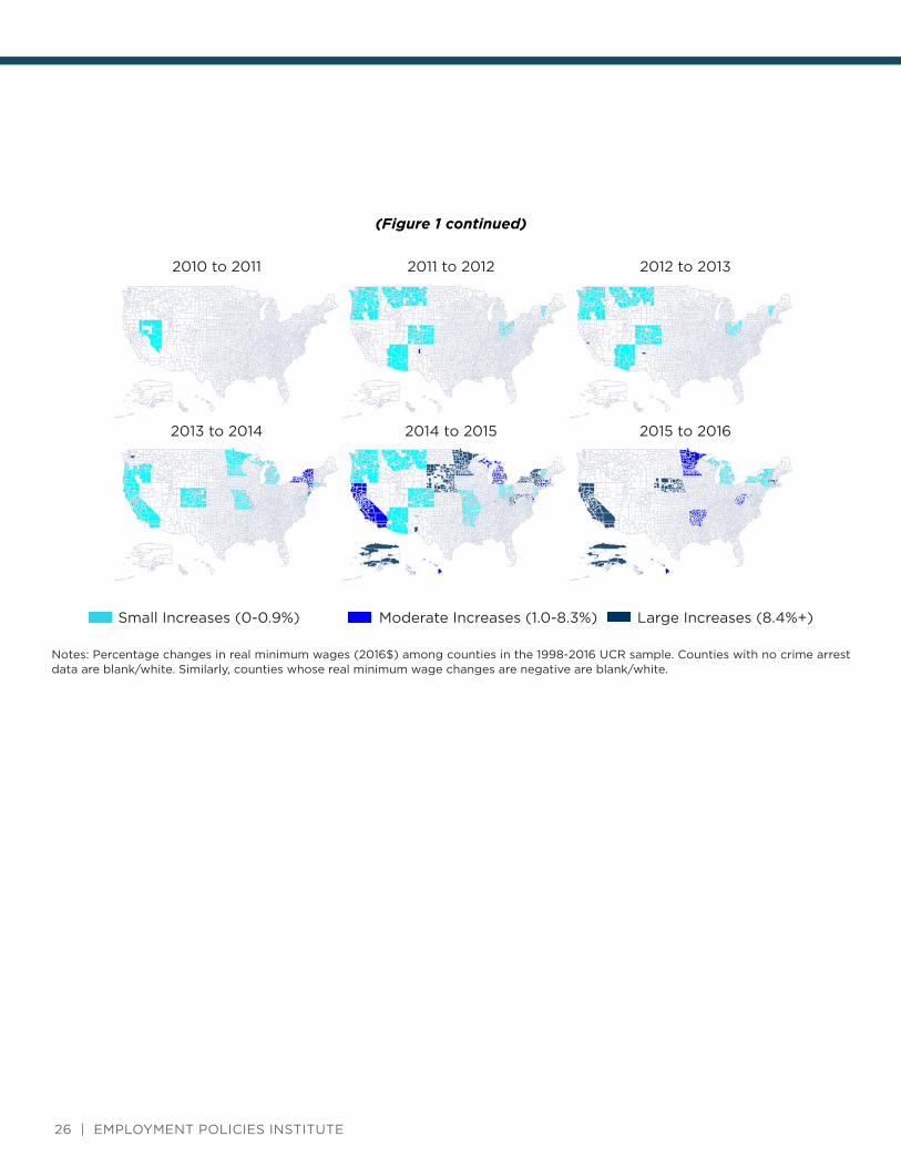
2010 to 2011 2011 to 2012 2012 to 2013

2013 to 2014 2014 to 2015 2015 to 2016


Notes: Percentage changes in real minimum wages (2016$) among counties in the 1998-2016 UCR sample. Counties with no crime arrest data are blank/white. Similarly, counties whose real minimum wage changes are negative are blank/white.

(Figure 1 continued)


Figure 2. Event Study of Estimated Relationship Between Changes in Minimum Wages and County-Level Property Crime Arrest Rates, Ages 16-to-24, UCR, 1998-2016

Notes: Estimates are generated using data from the 1998-2016 Uniform Crime Reports. Large changes are those in the top 25th percentile of the percentage increases of real minimum wages (9.0%). Moderate changes are those in the top 50th percentile of the percentage increases of real minimum wage (4.6%). Error bars are 90 percent confidence intervals.

Year from Minimum Wage Increase

Est

imate

d E

ffect

of

Min

imu

m W

ag

eIn

cre

ase

s o

n C

rim

e A

rrest

Rate

s



Est

imate

d E

ffect

of

Min

imu

m W

ag

eIn

cre

ase

s o

n C

rim

e A

rrest

Rate

s

Figure 3. Event Study of Estimated Relationship Between Changes in Minimum Wages and County-Level Violent Crime Arrest Rates, Ages 16-to-24, UCR, 1998-2016



Figure 4. Event Study of Estimated Relationship Between Changes in Minimum Wages and County-Level Drug Crime Arrest Rates, Ages 16-to-24, UCR, 1998-2016



Est

imate

d E

ffect

of

Min

imu

m W

ag

eIn

cre

ase

s o

n C

rim

e A

rrest

Rate

s


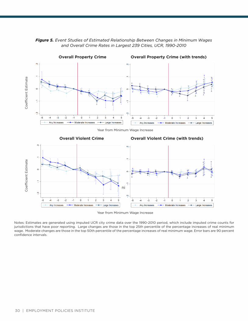
Figure 5. Event Studies of Estimated Relationship Between Changes in Minimum Wagesand Overall Crime Rates in Largest 239 Cities, UCR, 1990-2010

Notes: Estimates are generated using imputed UCR city crime data over the 1990-2010 period, which include imputed crime counts for jurisdictions that have poor reporting. Large changes are those in the top 25th percentile of the percentage increases of real minimum wage. Moderate changes are those in the top 50th percentile of the percentage increases of real minimum wage. Error bars are 90 percent confidence intervals.


Co

effi

cie

nt

Est

imate

Co

effi

cie

nt

Est

imate



Overall Property Crime Overall Property Crime (with trends)

Overall Violent Crime Overall Violent Crime (with trends)


Figure 6. Event Studies of Estimated Relationship Between Changes in Minimum Wages and Overall Crime Rates in Largest 239 Cities, UCR, 1990-1997

Notes: Estimates are generated using imputed UCR city crime data over the 1990-1997 period, which include imputed crime counts for jurisdictions that have poor reporting. Large changes are those in the top 25th percentile of the percentage increases of real minimum wage. Moderate changes are those in the top 75th percentile of the percentage increases of real minimum wage. Error bars are 90 percent confidence intervals.

Overall Property Crime

Overall Violent Crime

Co

effi

cie

nt

Est

imate


Co

effi

cie

nt

Est

imate



Table 1. Descriptive Statistics, Uniform Crime Reports, 1998-2016

Notes: Weighted means are generated using data from the 1998-2016 Uniform Crime Reports (UCR). Arrest rates are arrests per 1,000 people ages 16-to-24. Samples are restricted to counties with crime arrest rates within two standard deviations of the county’s average crime arrest rate, and counties with a coverage indicator of at least 65%. Standard deviations are in parentheses and number of observation in brackets. Means and standard deviations are weighted by the county population ages 16-to-24.

Mean(Standard Deviation)

Dependent Variables

Property Crime Arrest Rate, Ages 16-to-24Violent Crime Arrest Rate, Ages 16-to-24Drug Crime Arrest Rate, Ages 16-to-24

15.83 (9.80) [44,259]5.04 (6.38) [44,203]16.40 (16.12) [44,397]

Independent Variables

Minimum Wage (2016$)Socio-Demographic Controls

Number of reporting agenciesShares of malesShares of African AmericanShares of HispanicShares of individuals ages 25+ with a BA degree

Crime Policy ControlsShall issue lawsPolice expenditures per capita (2016$)Police employment per capita

Economic ControlsAverage hourly wages for adults ages 25-54 (2016$)Unemployment rates for males ages 25-54

Health and Social Welfare PoliciesState refundable EITCPresence of Medicaid for childless adultsSNAP all-vehicles exemptionMinimum dropout age of 18+E-verifyBan the box lawsMarijuana decriminalizationMedical marijuana lawsBeer taxes (2016+)

7.65 (0.87)

23.073 (25.398)0.492 (0.128)0.132 (0.136)0.162 (0.171)

0.293 (0.052)

0.626 (0.484)312.02 (84.24)2.291 (0.599)

22.92 (2.25)0.051 (0.023)

0.299 (0.458)0.110 (0.313)

0.600 (0.482)0.486 (0.500)0.166 (0.369)0.163 (0.360)0.178 (0.382)0.296 (0.452)

0.28 (0.23)


Table 2. Estimated Relationship Between Minimum Wages and Crime Arrest Rates for Those Ages 16-to-24, UCR, 1998-2016

Notes: Weighted OLS estimates are generated using data from the 1998-2016 Uniform Crime Reports. Arrest rates are arrests per 1,000 people ages 16-to-24. All regressions include controls for county fixed effects and year fixed effects. The list of socio-demographic controls, economic controls, crime policy controls and social welfare & health controls are available in Table 1. Samples are restricted to counties with crime arrest rates within two standard deviations of the county’s average crime arrest rate, and counties with a coverage indicator of at least 65%. Estimates are weighted by the county population ages 16-to-24. Standard errors are clustered at the state level.

(1) (2) (3) (4)

Panel I: Property Crime Arrest Rates

Ln(MW)

ElasticityN

4.138**(1.771)0.261

44,259

4.059**(1.908)0.256

44,259

3.983*(2.163)0.252

44,259

3.317**(1.617)0.210

44,259

Panel III: Violent Crime Arrest Rates

Ln(MW)

ElasticityN

0.772(0.667)0.153

44,203

0.821(0.646)0.163

44,203

0.861(0.628)

0.17144,203

0.551(0.740)0.109

44,203

Panel IV: Drug Crime Arrest Rates

Ln(MW)

ElasticityN

2.693(3.185)0.164

44,397

2.771(3.217)0.169

44,397

2.857(2.968)0.174

44,397

0.655(2.417)0.04044,397

Socio-Demographic ControlsCrime Policy Controls Economic ControlsSocial Welfare & Health Policies

YesNoNoNo

YesYesNoNo

YesYesYesNo

YesYesYesYes

***Significant at 1% level **Significant at 5% level *Significant at 10% level


Table 3A. Dynamic Estimates of the Relationship Between Changes in Minimum Wages and Crime Arrests for Those Ages 16-to-24, UCR, 1998-2016

Notes: Weighted OLS estimates are generated using data from the 1998-2016 Uniform Crime Reports. Arrest rates are arrests per 1,000 people ages 16-to-24. All regressions include controls for county fixed effects and year fixed effects. Samples are restricted to counties with crime arrest rates within two standard deviations of the county’s average crime arrest rate, and counties with a coverage indicator of at least 65%. Estimates are weighted by the county population ages 16-to-24. Standard errors are clustered at the state level.

(1) (2) (3) (4) (5) (6) (7) (8) (9)

Property Crime Arrest Rates Violent Crime Arrest Rates Drugs Crime Arrest Rates

∆Ln(MW)t-3 -3.233(2.448)

-1.468(0.964)

-5.459(4.145)

∆Ln(MW)t-2 -1.911(1.387)

-0.820(0.766)

-2.963(2.513)

∆Ln(MW)t-1 2.172(1.538)

-0.586(0.820)

-2.303(2.419)

∆Ln(MW)t 3.197**(1.216)

3.766**(1.758)

3.022*(1.667)

-0.243(0.397)

-0.088(0.496)

-0.439(0.523)

-2.430(1.802)

-1.030(1.651)

-1.214(2.016)

∆Ln(MW)t+1 5.741***(1.613)

0.312(0.583)

2.215(2.980)

∆Ln(MW)t+2 3.443(2.123)

0.202(0.542)

3.886(4.032)

∆Ln(MW)t+3 4.065(3.433)

0.237(0.858)

4.490(5.284)

N 42,538 28,792 28,792 42,423 28,644 28,644 42,489 28,754 28,754

Mean Arrest RateCumulative Effect

15.699 16.202 16.20213.299*(7.439)

5.007 5.034 5.034-2.563(2.482)

16.270 16.619 16.619-1.349

(10.772)

p-value of ∑ λleads=0 0.522 0.226 0.215



Table 3B. Sensitivity of Estimates to the Inclusion of Controls for State-Specific Time Trends, UCR, 1998-2016

Notes: Weighted OLS estimates are generated using data from the 1998-2016 Uniform Crime Reports. Arrest rates are arrests per 1,000 people ages 16-to-24. All regressions include controls for county fixed effects, year fixed effects, socio-demographic controls, economic controls, crime policy controls, and social welfare & health controls (available in Table 1). Samples are restricted to counties with crime arrest rates within two standard deviations of the county’s average crime arrest rate, and counties with a coverage indicator of at least 65%. Estimates are weighted by the county population ages 16-to-24. Standard errors are clustered at the state level.

(1) (2) (3) (4)


Ln(MW)

ElasticityN

5.182***(1.135)0.327

44,259

5.230***(1.076)0.33044,259

4.021***(0.970)0.254

44,259

3.300**(1.589)0.20844,259

Panel II: Violent Crime Arrest Rates

Ln(MW)

ElasticityN

0.481(0.648)0.09644,203

0.678(0.803)

0.13544,203

1.193*(0.683)0.237

44,203

1.721(1.179)0.342

44,203

Panel III: Drug Crime Arrest Rates

Ln(MW)

ElasticityN

1.315(2.285)0.08044,397

2.089(2.721)0.127

44,397

2.193(3.235)0.134

44,397

2.027(2.880)0.124

44,397

State-specific linear trendsState-specific quadratic trendsState-specific 3rd-order trendsState-specific 4th-order trends

YesNoNoNo

YesYesNoNo

YesYesYesNo

YesYesYesYes



Table 4. Heterogeneity in Relationship Between Minimum Wages and Property Crime Arrest Rates by Age Groups, UCR, 1998-2016

Notes: Weighted OLS estimates are generated using data from the 1998-2016 Uniform Crime Reports. Arrest rates are arrests per 1,000 people of the specified age group. All regressions include controls for county fixed effects, year fixed effects, socio-demographic controls, economic controls, crime policy controls, and social welfare & health controls. Regressions in columns (3)-(8) do not control for prime-age male unemployment rates, prime-age wage rates, or the share of individuals with a college degree to avoid controlling for mechanisms; instead, they control for the state-level housing price index. Samples are restricted to counties with crime arrest rates within two standard deviations of the county’s average crime arrest rate, and counties with a coverage indicator of at least 65%. Estimates are weighted by the county population of the specified age group. Standard errors are clustered at the state level.


(1) (2) (3) (4) (5) (6) (7) (8)

Ages 16-to-19

Ages 20-to-24

Ages 25-to-29

Ages 30-to-34

Ages 35-to-44

Ages 45-to-54

Ages 55-to-64

Ages 16-to-64

Panel I: Baseline Model

Ln(MW)

ElasticityN

3.261*(1.904)0.162

44,203

3.310**(1.619)0.27044,325

0.678(1.142)0.07844,310

0.215(1.068)0.03144,172

-0.943(0.898)-0.17844,277

-0.683*(0.365)-0.23644,248

-0.090(0.106)-0.08944,052

0.564(0.772)0.08444,526

Panel II: With State-Specific Quadratic Time Trends

Ln(MW)

ElasticityN

5.541***(1.182)0.274

44,203

4.766***(1.275)0.38944,325

1.252*(0.640)

0.14544,310

0.824(0.660)

0.11744,172

0.077(0.532)0.014

44,277

0.077(0.225)0.02644,248

0.135(0.082)0.134

44,052

1.048**(0.467)0.157

44,526

Panel III: With State-Specific 4th-Order Time Trends

Ln(MW)

ElasticityN

3.708(2.243)0.184

44,203

3.147**(1.314)0.257

44,325

1.328(1.286)0.154

44,310

0.837(1.219)0.119

44,172

0.117(0.909)0.02244,277

-0.044(0.328)-0.01544,248

0.074(0.101)0.07444,052

1.111(0.803)0.166

44,526


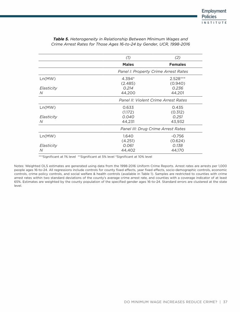
Table 5. Heterogeneity in Relationship Between Minimum Wages and Crime Arrest Rates for Those Ages 16-to-24 by Gender, UCR, 1998-2016

Notes: Weighted OLS estimates are generated using data from the 1998-2016 Uniform Crime Reports. Arrest rates are arrests per 1,000 people ages 16-to-24. All regressions include controls for county fixed effects, year fixed effects, socio-demographic controls, economic controls, crime policy controls, and social welfare & health controls (available in Table 1). Samples are restricted to counties with crime arrest rates within two standard deviations of the county’s average crime arrest rate, and counties with a coverage indicator of at least 65%. Estimates are weighted by the county population of the specified gender ages 16-to-24. Standard errors are clustered at the state level.

(1) (2)

Males Females


Ln(MW)

ElasticityN

4.394*(2.485)0.214

44,200

2.528***(0.940)0.23644,201


Ln(MW)

ElasticityN

0.633(1.172)0.04044,231

0.435(0.312)0.251

43,932


Ln(MW)

ElasticityN

1.640(4.251)0.061

44,402

-0.756(0.624)0.138

44,170



Table 6. Heterogeneity in Relationship Between Minimum Wages and Crime Arrest Rates for Those Ages 16-to-24 by Specific Type of Crime, UCR, 1998-2016



(1) (2) (3) (4)

Panel I: Specific Property Crimes

Burglary LarcenyMotor

Vehicle TheftArson

Ln(MW)

ElasticityN

-0.087(0.372)-0.02944,023

2.764***(0.939)0.241

44,272

0.746(0.595)0.66443,826

0.016(0.018)0.198

43,708

Panel II: Specific Violent Crimes

AggravatedAssault

Robbery Murder Rape

Ln(MW)

ElasticityN

0.338(0.539)0.10344,161

0.160(0.247)

0.11444,002

0.026(0.030)0.184

43,839

0.013(0.046)0.06943,803

Panel III: Minor Crimes

Vandalism Liquor Laws DrunkennessDisorderlyConducts

Ln(MW)

ElasticityN

0.493(0.367)

0.1944,019

3.481(3.181)0.38244,105

-0.715(1.040)-0.20944,495

3.389*(1.794)0.61944,183


Table 7. Estimated Relationship Between Living Wages and Crime Arrest Rates for Those Ages 16-to-24, UCR, 1998-2016


(1) (2) (3)

Property Crime Arrest Rates

Violent Crime Arrest Rates

Drug Crime Arrest Rates

Ln(MW)

Elasticity

Living Wage

%Δ associated with law

Living Wage*Financial Assisstance

%Δ associated with law

N

3.298**(1.635)0.208

-0.935(0.710)-0.059

1.462*(0.789)0.092

44,259

0.480(0.758)0.095

0.501**(0.245)0.099

0.246(0.389)0.049

44,203

0.589(2.407)0.036

-0.053(1.117)

-0.003

1.162(0.908)0.071

44,397



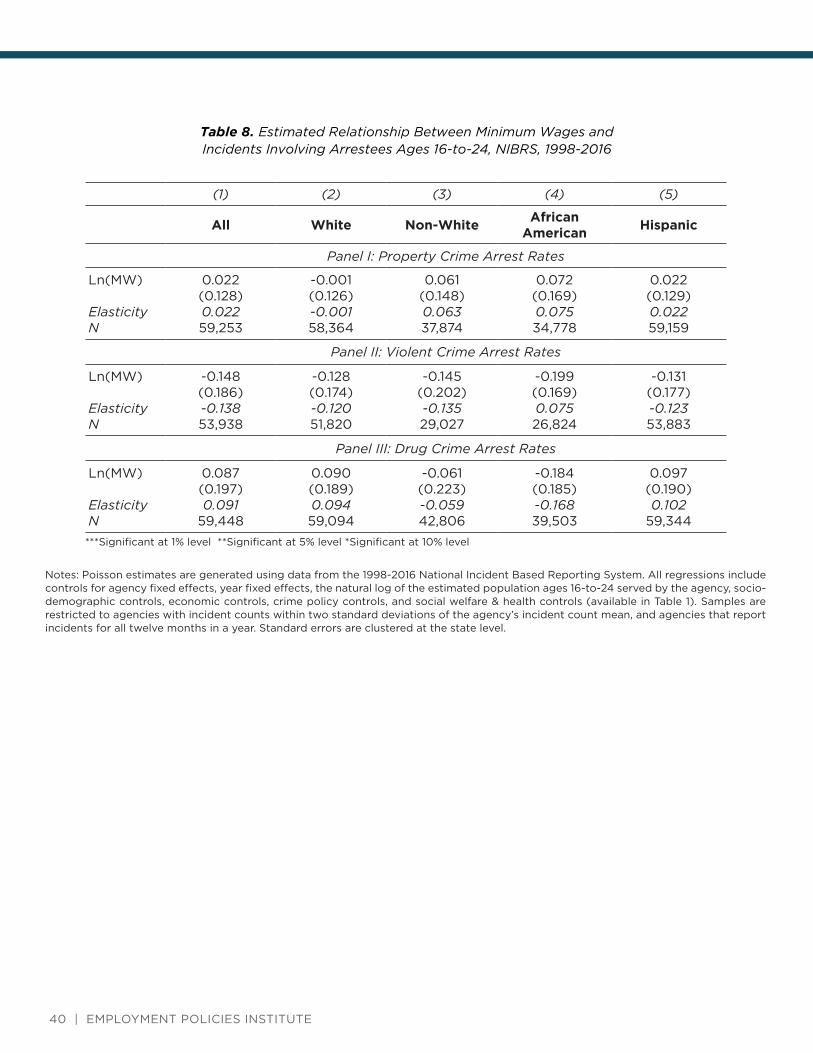
Table 8. Estimated Relationship Between Minimum Wages and Incidents Involving Arrestees Ages 16-to-24, NIBRS, 1998-2016

Notes: Poisson estimates are generated using data from the 1998-2016 National Incident Based Reporting System. All regressions include controls for agency fixed effects, year fixed effects, the natural log of the estimated population ages 16-to-24 served by the agency, socio-demographic controls, economic controls, crime policy controls, and social welfare & health controls (available in Table 1). Samples are restricted to agencies with incident counts within two standard deviations of the agency’s incident count mean, and agencies that report incidents for all twelve months in a year. Standard errors are clustered at the state level.


(1) (2) (3) (4) (5)

All White Non-WhiteAfrican

AmericanHispanic


Ln(MW)

ElasticityN

0.022(0.128)0.02259,253

-0.001(0.126)-0.00158,364

0.061(0.148)0.06337,874

0.072(0.169)0.07534,778

0.022(0.129)0.02259,159


Ln(MW)

ElasticityN

-0.148(0.186)-0.13853,938

-0.128(0.174)-0.12051,820

-0.145(0.202)-0.13529,027

-0.199(0.169)0.07526,824

-0.131(0.177)-0.12353,883


Ln(MW)

ElasticityN

0.087(0.197)0.091

59,448

0.090(0.189)0.09459,094

-0.061(0.223)-0.05942,806

-0.184(0.185)-0.16839,503

0.097(0.190)0.102

59,344


Table 9. Estimated Relationship Between Minimum Wages and Crime Arrest Rates for Those Ages 16-to-24 by Jurisdiction Size, UCR, 1998-2016

Notes: Weighted OLS estimates are generated using data from the 1998-2016 Uniform Crime Reports. Arrest rates are arrests per 1,000 people of the specified age group. All regressions include controls for county fixed effects, year fixed effects, socio-demographic controls, economic controls, crime policy controls, and social welfare & health controls (available in Table 1). Samples are restricted to counties with crime arrest rates within two standard deviations of the county’s average crime arrest rate, and counties with a coverage indicator of at least 65%. Estimates are weighted by the county population ages 16-to-24. Standard errors are clustered at the state level.


(1) (2) (3) (4)

NIBRSCounties

Population≥ 100,000

Population25,000-100,000

Population< 25,000


Ln(MW)

ElasticityN

1.753(1.660)0.115

18,303

3.820**(1.718)0.2408,485

2.099(1.996)0.12515,152

0.651(1.932)0.05920,622


Ln(MW)

ElasticityN

-1.167(0.763)-0.30917,543

0.747(0.931)0.1418,525

0.555(0.698)

0.12715,091

0.509(1.060)0.162

20,587


Ln(MW)

ElasticityN

-0.734(2.645)-0.05118,333

1.827(3.163)0.1108,548

-1.754(2.948)-0.10715,188

1.835(3.387)0.137

20,661


Table 10. Estimated Relationship Between Minimum Wages and Labor Market Outcomes and School Enrollment for those ages 16-to-24 without a High School Diploma, CPS, 1998-2016

(1) (2) (3) (4)

Panel I: Property Crime Arrest RatesLn(MW)

N

0.184***(0.033)83,731

0.184***(0.033)83,731

0.185***(0.028)83,731

0.176***(0.032)83,731

Panel II: Violent Crime Arrest RatesLn(MW)

ElasticityN

-0.040(0.041)-0.147

293,216

-0.043(0.034)-0.158

293,216

-0.042(0.034)-0.154

293,216

-0.059**(0.029)-0.217

293,216Panel III: Drug Crime Arrest Rates

Ln(MW)

ElasticityN

-1.412(1.002)-0.204293,216

-1.508*(0.813)-0.218

293,216

-1.496*(0.820)-0.217

293,216

-1.885*(0.810)-0.273293,216

Panel IV: Ln(Weekly Hours) | EmploymentLn(MW)

N

-0.078(0.064)83,731

-0.082(0.058)83,731

-0.079(0.057)83,731

-0.084(0.054)83,731

Panel V: Usual Weekly EarningsLn(MW)

ElasticityN

0.351(11.767)0.005

293,216

-0.704(9.227)-0.010293,216

-0.533(9.382)-0.008293,216

-4.979(9.539)-0.072293,216

Panel VI: School EnrollmentLn(MW)

ElasticityN

-0.034(0.037)-0.04595,674

-0.030(0.037)-0.03995,674

-0.030(0.037)-0.03995,674

-0.034(0.037)-0.04595,674

Panel VII: School Enrollment and EmploymentLn(MW): Enrolled, Employed

Ln(MW): Enrolled, Not Employed

Ln(MW): Not Enrolled, Employed

Ln(MW): Not Enrolled, Not Employed

N

-0.012(0.040)-0.003(0.039)0.016

(0.024)-0.000(0.027)95,674

-0.013(0.036)0.000

(0.035)0.012

(0.022)0.000

(0.026)95,674

-0.009(0.037)-0.004(0.036)0.013

(0.021)0.000

(0.025)95,674

-0.023(0.037)0.005

(0.037)0.020

(0.024)-0.001

(0.028)95,674

Socio-demographic controlsCrime policy controlsEconomic controlsSocial welfare & health policies

YesNoNoNo

YesYesNoNo

YesYesYesNo

YesYesYesYes

Notes: Data are drawn from the 1998-2016 Current Population Survey (CPS) Outgoing Rotation Groups (ORG) for Panels I-V and the CPS October Supplement for Panels VI and VII. All regressions include state fixed effects, year fixed effects, month fixed effects, economic controls, crime policy controls and social welfare & health controls (as noted in Table 1). Panels I, III, IV, and V are estimated via OLS; Panels II and VI are estimated via probit; and Panel VII is estimated via multinomial logit. Estimates are weighted using the sample weights provided by the CPS, and standard errors corrected for clustering on the state are in parentheses.



Table 11. Estimated Relationship between Minimum Wage and Crime, NLSY97, 1998-2016

Notes: Weighted estimates are generated using data from the 1998-2016 National Longitudinal Survey of Youth 1997 (NLSY97). All regressions include controls for state fixed effects, individual characteristics (available in Appendix Table 2), socio-demographic controls, economic controls, crime policy controls, and social welfare & health controls (available in Table 1). Standard errors are clustered at the state level.


(1)Any Crime

(2)Property

(3)Violent

(4)Sold Drugs

(5)Arrest

Ages 16-to-24

Ages 25+

NR-squared

0.018**(0.008)0.019**(0.009)

51,0670.056

0.017***(0.006)0.026***(0.007)

51,0660.047

-0.003(0.007)0.006

(0.007)

45,7300.018

-0.000(0.008)0.003

(0.009)

51,0690.015

0.004(0.005)0.020***(0.007)

71,8800.007



Table 12. Estimates Relationship between Minimum Wage and Labor Market Outcomes, NLSY97, 1998-2016



(1)Total Weeks Worked

(2) Hours Per Week

(3)Total Hours Worked

(4)Employed

Ages 16-to-24

Ages 25+

NR-squared

-1.264*(0.731)

-6.320***(0.849)

71,7410.439

-1.619***(0.427)

-4.461***(0.476)

67,3310.117

-114.047***(30.151)

-401.732***(40.948)

67,3310.43

0.008(0.006)

-0.035***(0.009)

72,3650.009

Table 13. Estimated Relationship between Minimum Wage and Crime, Below and Above Median Annual Hours Worked Samples, NLSY97, 1998-2016

Notes: Weighted estimates are generated using data from the 1998-2016 National Longitudinal Survey of Youth 1997 (NLSY97). All regressions include controls for state fixed effects, age dummies, individual characteristics (available in Appendix Table 2), socio-demographic controls, economic controls, crime policy controls, and social welfare & health controls (available in Table 1). Standard errors are clustered at the state level.


(1)Any Crime

(2)Property Crime

(3)Assault

(4)Sold Drugs

(5)Arrest

Panel I: Below Median Annuals Hours Worked

Ages 16-to-24

Ages 25+

NR-squared

0.032**(0.013)0.015

(0.016)

23,6620.045

0.026***(0.008)0.033*(0.017)

23,6620.042

0.001(0.010)0.000(0.014)

22,9220.015

0.002(0.013)-0.002(0.012)

23,6610.012

0.007(0.006)0.000(0.012)

30,2780.006

Panel II: Above Median Annuals Hours Worked

Ages 16-to-24

Ages 25+

NR-squared

-0.009(0.016)0.016

(0.013)

27,4050.058

-0.002(0.013)0.018**(0.009)

27,4040.044

-0.011(0.010)0.007

(0.009)

22,8080.028

-0.004(0.009)0.003

(0.010)

27,4080.019

-0.004(0.010)0.029***(0.010)

41,6020.010



Table 14. Sensitivity of Results to Large City Aggregate Crime Rates for 1990-2010 Period Examined by Fernandez et al. (2014)

(1) (2) (3) (4) (5)

Panel I: Ln(Overall Property Crime Rates)

Ln(MW)

N

-0.500***(0.118)4,710

-0.094(0.133)4,710

-0.024(0.054)

4,710

0.026(0.062)4,710

0.030(0.109)4,710

Panel II: Ln(Overall Violent Crime Rates)

Ln(MW)

N

-0.802***(0.102)4,560

-0.237(0.142)4,560

-0.092(0.071)4,560

-0.092(0.098)4,560

-0.011(0.120)4,560

City & Year FEs Controls City Linear Time TrendsCity Quadratic Time TrendsCity 4th-Order Time Trends

YNNNN

YYNNN

YYYNN

YYYYN

YYYYY

Notes: Weighted OLS estimates are generated using imputed UCR city crime data over the 1990-2010 period, which include imputed crime counts for jurisdictions that have poor reporting. Controls from Fernandez et al. (2014) include the percent of the county population that is African American, white, female, ages 0-19, 20-29, 30-39, 40-49, and 50-64, as well city-level log of police per capita, the state-level log of imprisonment rates, adult unemployment rates, and per capita personal income. Estimates are weighted by city population, and standard errors are clustered at the state level.


Table 15. Sensitivity of Results to Aggregate Crime Rates for States and Years in NCRP Data Examined by Agan and Makowsky (2018)

a Estimates from columns (1)-(2) use imputed UCR crime, which include imputed crime counts for jurisdictions that have poor reporting.b Estimates from columns (3)-(8) use data from the UCR’s Arrests by Age, Sex, and Race files, the data which we have used for Tables 1-7 and 9.

Notes: Weighted OLS estimates are generated using data from the 2000-2016 Uniform Crime Reports. Arrest rates are arrests per 1,000 people of the specified age group. All regressions include controls for county fixed effects, year fixed effects, the number of agencies reporting to a county, county level percent male, African American, white, ages 0-19, 20-29, 30-39, 40-49, and 50-64, as well as state level police per capita, state level housing price index, the share of individuals with a college degree, an indicator for whether the governor is democrat, whether drug convicts are eligible for TANF benefits, whether parolees are eligible to vote, and the presence of a state EITC top-up. Samples are restricted to counties with crime arrest rates within two standard deviations of the county’s average crime arrest rate, and counties with a coverage indicator of at least 65%. Estimates are weighted by the county population of the specified age group. Standard errors are clustered at the state level.


(1) (2) (3) (4) (5) (6) (7) (8)

All Agesa

Ages 18+b

Male Ages 18+b African American

Ages 18+b


Ln(MW)

ElasticityN

0.118(0.075)0.155

24,287

0.083(0.106)

0.11735,586

0.024(0.078)0.03635,492

0.059(0.066)0.09040,584

0.001(0.119)0.001

35,448

0.076(0.099)0.08640,542

-0.031(0.202)-0.01934,957

0.140(0.164)0.09040,005


Ln(MW)

ElasticityN

0.021(0.026)0.09024,283

0.083(0.053)0.32635,599

0.057(0.045)

0.21135,411

0.062(0.037)0.237

40,437

0.091(0.075)0.201

35,365

0.089(0.062)0.20440,398

0.044(0.169)0.05234,970

0.141(0.140)0.176

39,999


Ln(MW)

ElasticityN

-0.098(0.064)-0.13724,287

0.095(0.097)0.13335,621

0.085(0.103)0.108

35,470

0.040(0.113)0.05240,451

0.152(0.178)0.117

35,452

0.094(0.190)0.075

40,464

0.310(0.731)0.143

34,952

0.145(0.596)0.071

39,950

YearsStates

2000-2014NCRP States

2000-2014UCR States

2000-2014UCR States

2000-2016UCR States

2000-2014UCR States

2000-2016UCR States

2000-2014UCR States

2000-2016UCR States


Appendix Figure 1. Identifying Variation in Real Minimum Wages from UCR Sampled Counties, 1989-1998

Notes: Percentage changes in real minimum wages (2016$) among counties in the 1990-1998 UCR sample. Counties with no crime arrest data are blank/white. Similarly, counties whose real minimum wage changes are negative are blank/white.

1989 to 1990 1990 to 1991 1991 to 1992

1992 to 1993 1993 to 1994 1994 to 1995

1995 to 1996 1996 to 1997 1997 to 1998



Year from Living Wage Enactment

Co

effi

cie

nt

Est

imate

Appendix Figure 2. Event Study of Estimated Relationship Between Living Wage Laws covering Financial Assistance Recipients and County-Level Property Crime Arrest Rates, Ages 16-to-24, UCR, 1998-2016

Notes: Estimates are generated using data from the 1998-2016 Uniform Crime Reports. Controls are included for the living wage main effect, minimum wages, county fixed effects, and year fixed effects. Error bars are 90 percent confidence intervals.


Appendix Table 1A. Descriptive Statistics of Crime Arrest Rates by Age and Gender, UCR, 1998-2016

Notes: Weighted means and standard deviations are generated using data from the 1998-2016 Uniform Crime Reports. Samples are restricted to counties with crime arrest rates within two standard deviations of the county’s average crime arrest rate, and counties with a coverage indicator of at least 65%. Standard deviations are in parentheses and number of observation in brackets. Means and standard deviations are weighted using the county population of specified age (and gender) group.

(1) (2) (3)

Property Crime Arrest Rates

Violent Crime Arrest Rates

Drug Crime Arrest Rates

Ages 16-19

Ages 20-24

Ages 25-29

Ages 30-34

Ages 35-44

Ages 45-54

Ages 55-64

Ages 16-64

20.15 (13.06)[44,203]

12.25 (7.85)[44,325]

8.64 (6.86)[44,310]

7.04 (6.09)[44,172]

5.31 (4.79)[44,277]

2.90 (2.59)[44,248]

1.01 (0.86)[44,052]

6.69 (4.52)[44,526]

5.11 (7.29)[44,157]

4.97 (5.97)[44,117]

3.91 (5.51)[44,097]3.12 (4.11)[44,063]

2.32 (3.16)[44,101]

1.21 (1.55)[44,060]

0.44 (0.56)[43,907]

2.56 (3.35)[44,357]

16.23 (16.63)[44,348]

16.40 (15.65)[44,284]

11.25 (12.68)[44,246]

8.40 (10.31)[44,072]

6.01 (8.43)[44,162]

3.02 (4.48)[44,213]

0.85 (1.40)[43,885]

7.374 (8.28)[44,364]

Ages 16-24

Males

Females

20.49 (13.35)[44,200]

10.71 (7.10)[44,201]

8.18 (10.65)[44,231]

1.73 (2.30)[43,932]

26.73 (28.78)[44,402]

5.50 (4.20)[44,170]


Appendix Table 1B. Descriptive Statistics of Crime Arrest Rates for Those Ages 16-to-24, by Type of Crime, UCR, 1998-2016

Notes: Weighted means and standard deviations are generated using data from the 1998-2016 Uniform Crime Reports. Samples are restricted to counties with crime arrest rates within two standard deviations of the county’s average crime arrest rate, and counties with a coverage indicator of at least 65%. Standard deviations are in parentheses and number of observation in brackets. Means and standard deviations are weighted using the county population of the specified age (and gender) group.

(1) (2) (3) (4)

Burglary Larceny Motor vehicle theft Arson

3.047 (2.20) [44,023]

11.485 (7.45) [44,272]

1.124 (2.01) [43,826]

0.081 (0.145) [43,708]

Aggravated Assault Robbery Murder Rape

3.266 (3.59) [44,161]

1.401 (2.69) [44,002]

0.141 (0.26) [43,839]

0.189 (0.26)[43,803]

Vandalism Liquor laws Drunkenness Disorderly conducts

2.60 (2.200)[44,019]

9.12 (13.69)[44,105]

3.43 (5.40) [44,495]

5.48 (7.53) [44,183]


Appendix Table 1C. Descriptive Statistics of Crime Incidents, NIBRS, 1998-2016

Notes: Weighted means and standard deviations are generated using data from the 1998-2016 National Incident Based Reporting System (NIBRS). Samples are restricted to agencies with incident counts within two standard deviations of the agency’s incident count mean, and agencies that report incidents for all twelve months in a year. Standard deviations are in parentheses and number of observations in brackets. Means and standard deviations are weighted using the agency population of the specified age group.

(1) (2) (3) (4) (5) (6) (7) (8) (9) (10) (11) (12)

Ages 16-to-24

All White Non-WhiteAfrican

AmericanHispanic

Ages 16-to-19

Ages 20-to-24

Ages 25-to-29

Ages 30-to-34

Ages 35-to-44

Ages 45-to-54

Ages 55-to-64


213.63 (381.91)[59,253]

117.75(197.83)[58,364]

190.08 (383.39) [37,874]

212.38(414.99)[34,778]

305.15(468.75)[59,159]

118.45 (219.07)[56,755]

106.13 (186.84)[56,563]

86.25 (148.20)[54,727]

67.55 (120.14)[53,228]

99.96 (192.54)[55,534]

61.70 (129.19)[51,184]

18.95(40.71)[38,126]


70.36 (162.94) [53,938]

24.68 (41.61)

[51,820]

101.28 (223.21)[29,027]

117.81(242.61)26,824

89.21(170.08)[53,883]

33.69 (84.52)

[46,362]

42.48 (92.95)[49,651]

35.39 (71.26)

[48,233]

26.29 (53.18)

[46,145]

36.15 (76.84)

[50,780]

22.04 (51.94)

[45,204]

7.47 (18.04)

[30,403]


201.27 (404.60)[59,448]

98.63 (171.95)

[59,094]

209.56 (48.24)

[42,806]

241.56(486.64)[39,503]

280.53(469.36)[59,334]

88.69 (180.39)[57,159]

123.74 (247.67)[57,955]

97.28 (193.08)[56,764]

66.04 (133.28)[55,094]

75.50 (151.42)[56,658]

37.76 (77.97)

[53,900]

10.13 (22.09)[39,701]


Appendix Table 2. Descriptive Statistics of Selected Variables, NLSY, 1998-2016

Notes: Estimates are generated using data from the 1998-2016 National Longitudinal Study of Youth 1997 (NLSY97). Reported observations correspond to maximum sample size. Because of missing observations, the sample size is smaller for some variables.

(1) (2) (3)

All Ages 16-to-24 Ages 25+

Crime and Arrest

Any Crime

Property Crime

Sold Drugs

Assault

Arrest

0.10(0.31)0.06

(0.24)0.04

(0.20)0.04

(0.20)0.04

(0.20)

0.14(0.35)0.08

(0.28)0.05

(0.22)0.05

(0.22)0.05

(0.22)

0.04(0.20)0.02(0.14)0.02(0.15)0.02(0.13)0.03(0.17)

Labor Market Outcomes

Hours Per Week

Total Weeks Worked

Total Hours Worked

Hourly Wage

Employed

33.79(13.27)45.02(27.22)1,670.28

(1,234.72)17.76

(412.15)0.94

(0.25)

30.68(13.22)36.66(18.83)1,213.82(773.97)

13.45(236.36)

0.93(0.25)

37.30(12.42)54.65(31.81)

2,186.00(1,438.35)

22.65(546.86)

0.94(0.24)

Individual Characteristics

Minimum Wage Bound

Non-Black, non-Hispanic

Maternal Education

Math PIAT Score

Household Income 1997

N

0.029(0.165)

0.52(0.50)12.50(2.92)97.64

(19.27)46,836.23(41,169.69)

71,702

0.036(0.183)0.54

(0.50)12.54(2.90)98.33

(19.08)47,427.43

(41,333.50)38,376

0.018(0.135)

0.51(0.50)12.46(2.94)96.72

(19.47)46,142.21

(40,966.52)33,326


Appendix Table 3. Estimated Relationship Between Minimum Wages and Control Variables

(1) (2) (3)

Property CrimeArrest Rates

Violent CrimeArrest Rates

Drug CrimeArrest Rates

Number of reporting agencies

Shares of males

Shares of African American

Shares of Hispanic

Shares of individuals ages 25+ with a BA degree

Shall issue laws

Ln(police expenditures per capita)

Ln(police employment per capita)

Ln(prime-age hourly wages)

Ln(prime-age male unemployment rates)

State refundable EITC

0.057(0.125)20.946(39.216)17.459*(9.985)-12.761(7.999)11.249

(9.885)

-0.341(0.772)

1.181(2.488)1.074

(1.632)-6.083(5.972)0.763

(0.588)

0.754(0.612)

-0.108(0.079)13.054

(24.602)14.371*(7.332)5.624

(7.405)-6.010

(3.640)

0.528**(0.213)

1.155(0.893)-1.095**(0.480)

2.811(2.516)-0.259(0.187)

-0.348*(0.187)

-0.180(0.346)69.679(91.567)44.694(27.707)18.659

(26.833)-18.155

(16.690)

0.961(0.785)0.805

(2.705)-1.623

(2.029)8.285

(6.859)-1.478**(0.607)

-0.909*(0.486)

Presence of Medicaid for childless adults

SNAP all-vehicles exemption

Minimum dropout age of 18+

E-verify

Ban the box laws

Marijuana decriminalization

Medical marijuana laws

Ln(beer taxes)

N

-0.288(0.473)-0.046(0.366)0.096

(0.795)0.516

(0.545)0.393

(0.546)-1.860***(0.630)-0.022(0.660)0.768

(0.515)44,259

-0.187(0.413)-0.168(0.151)0.478**(0.208)0.038(0.148)-0.430*(0.229)-0.521

(0.333)0.273

(0.301)0.375***(0.124)44,203

-1.046(1.305)0.398

(0.458)1.283**(0.609)0.022

(0.481)-1.488*(0.830)-5.147***(1.038)0.566(1.027)-0.344(0.628)44,397


Notes: Weighted OLS estimates are generated using data from the 1998-2016 Uniform Crime Reports. Arrest rates are arrests per 1,000 people ages 16-to-24. Samples are restricted to counties with crime arrest rates within two standard deviations of the county’s average crime arrest rate, and counties with a coverage indicator of at least 65%. Estimates are weighted by the county population ages 16-to-24. Standard errors are clustered at the state level.


Appendix Table 4. Heterogeneity in Relationship Between Minimum Wages and Crime Arrest Rates by Age Groups, UCR, 1998-2016

Notes: Weighted OLS estimates are generated using data from the 1998-2016 Uniform Crime Reports. Arrest rates are arrests per 1,000 people of the specified age group. All regressions include controls for county fixed effects, year fixed effects, socio-demographic controls, economic controls, crime policy controls, and social welfare & health controls. Regressions in columns (3)-(8) do not control for prime-age male unemployment rates, prime-age wage rates, or the share of individuals with a college degree to avoid controlling for mechanisms; instead, they control for the state-level price housing index. Samples are restricted to counties with crime arrest rates within two standard deviations of the county’s average crime arrest rate, and counties with a coverage indicator of at least 65%. Estimates are weighted by the county population of the specified age group. Standard errors are clustered at the state level.

(1) (2) (3) (4) (5) (6) (7) (8)

Ages 16-to-19

Ages 20-to-24

Ages 25-to-29

Ages 30-to-34

Ages 35-to-44

Ages 45-to-54

Ages 55-to-64

Ages 16-to-64

Panel I: Violent Crime Arrest Rates

Ln(MW)

ElasticityN

-0.038(0.940)-0.00744,157

0.779(0.660)

0.15744,117

0.357(0.710)0.09144097

0.254(0.654)0.081

44,063

0.009(0.439)0.00444,101

0.045(0.201)0.037

44,060

0.048(0.079)0.108

43,907

0.208(0.465)0.081

44,357

Panel II: Drug Crime Arrest Rates

Ln(MW)

ElasticityN

-1.312(2.483)-0.08144,348

1.469(2.333)0.09044,284

-0.823(1.414)-0.07344,246

0.292(1.919)0.03544,072

0.333(1.684)0.05544,162

-0.265(0.674)-0.08844,213

0.178(0.189)0.210

43,885

0.150(1.479)0.02044,357



Appendix Table 5. Exploiting Variation in the Bindingness of Federal Minimum Wage Increases, ages 16-to-24, UCR, 1998-2016

Property Violent Drug

Ln(MW)

Elasticity

Ln(MW)*Bound

Elasticity

Bound

N

4.752**(1.798)

0.300

1.454(3.741)0.092

-1.424(7.266)

44,259

0.666(0.931)

0.132

-0.842(1.130)-0.167

1.665(2.290)

44,203

1.650(2.806)

0.101

-2.389(3.934)-0.146

5.333(7.649)

44,397




Appendix Table 6. Heterogeneity in Relationship Between Minimum Wages and Incidents by Age Groups of Arrestees, NIBRS, 1998-2016


Notes: Poisson estimates are generated using data from the 1998-2016 National Incident Based Reporting System. All regressions include controls for agency fixed effects, year fixed effects, socio-demographic controls, economic controls, crime policy controls, and social welfare & health controls. Regressions in columns (3)-(7) do not control for prime-age male unemployment rates, prime-age wage rates, or the share of individuals with a college degree to avoid controlling for mechanisms; instead, they control for the state-level housing index. Samples are restricted to agencies with incident counts within two standard deviations of the agency’s incident count mean, and agencies that report incidents for all twelve months in a year. Standard errors are clustered at the state level.

(1) (2) (3) (4) (5) (6) (7)

Ages 16-to-19

Ages 20-to-24

Ages 25-to-29

Ages 30-to-34

Ages 35-to-44

Ages 45-to-54

Ages 55-to-64


Ln(MW)

ElasticityN

0.094(0.120)0.09956,755

-0.037(0.143)-0.03656,563

-0.031(0.155)-0.03154,727

0.056(0.138)0.05853,228

-0.066(0.150)-0.06455,534

-0.172(0.134)-0.15851,184

-0.167(0.117)-0.15438,126


Ln(MW)

ElasticityN

-0.052(0.158)-0.05146,362

-0.215(0.217)-0.19349,651

-0.112(0.182)-0.10648,233

-0.113(0.248)-0.10746,145

-0.138(0.196)-0.12950,780

-0.014(0.182)-0.01445,204

0.030(0.211)0.03030,403


Ln(MW)

ElasticityN

0.201(0.210)0.22357,159

-0.012(0.217)-0.01257,955

-0.033(0.197)-0.03256,764

0.077(0.207)0.08055,094

0.041(0.183)0.04256,658

-0.082(0.203)-0.07953,900

0.256(0.265)0.29239,701


Appendix Table 7. Descriptive Statistics of Labor Market Outcomes and School Enrollment for Those Ages 16-to-24, CPS, 1998-2016

Notes: Weighted means and standard errors in Panel I are generated using data from the 1998-2016 Current Population Survey (CPS) Outgoing Rotation Groups (ORG). Weighted means and standard errors in Panel II are generated using data from the 1998-2016 CPS October Supplement. Standard deviations are in parentheses and number of observations in brackets.

Panel I: Labor Market Outcomes

Hourly Earnings (2016$) | Employment

Employment

Usual Weekly Hours

Usual Weekly Hours | Employment

Usual Weekly Earnings (2016$)

9.37 (4.52)[83,731]

0.272 (0.445)[293,216]

6.905 (13.241)[293,216]

25.423 (13.217)[83,731]

69.149 (153.96)[293,216]

Panel II: School Enrollment

School Enrollment

Enrolled, Employed

Enrolled, Not Employed

Not Enrolled, Employed

Not Enrolled, Not Employed

0.763 (0.425)[95,674]

0.180 (0.384)[95,674]

0.584 (0.493)[95,671]

0.121 (0.326)[95,671]

0.116 (0.320)[95,671]


Appendix Table 8. Estimated Relationship between Minimum Wage Bindingness and Criminal Engagement, Including Individual Fixed Effects, NLSY97, 1998-2016



(1) (2) (3) (4) (5)

Any Crime Property Violent Sold Drugs Arrest

Ages 16-to-24

Ages 25+

NR-squared

0.005(0.011)0.008(0.011)

51,0670.381

0.007(0.011)0.017

(0.010)

51,0660.305

-0.010(0.007)-0.001

(0.009)

45,7300.293

-0.004(0.009)0.001

(0.010)

51,0690.345

0.002(0.006)0.000

(0.008)

71,8800.251


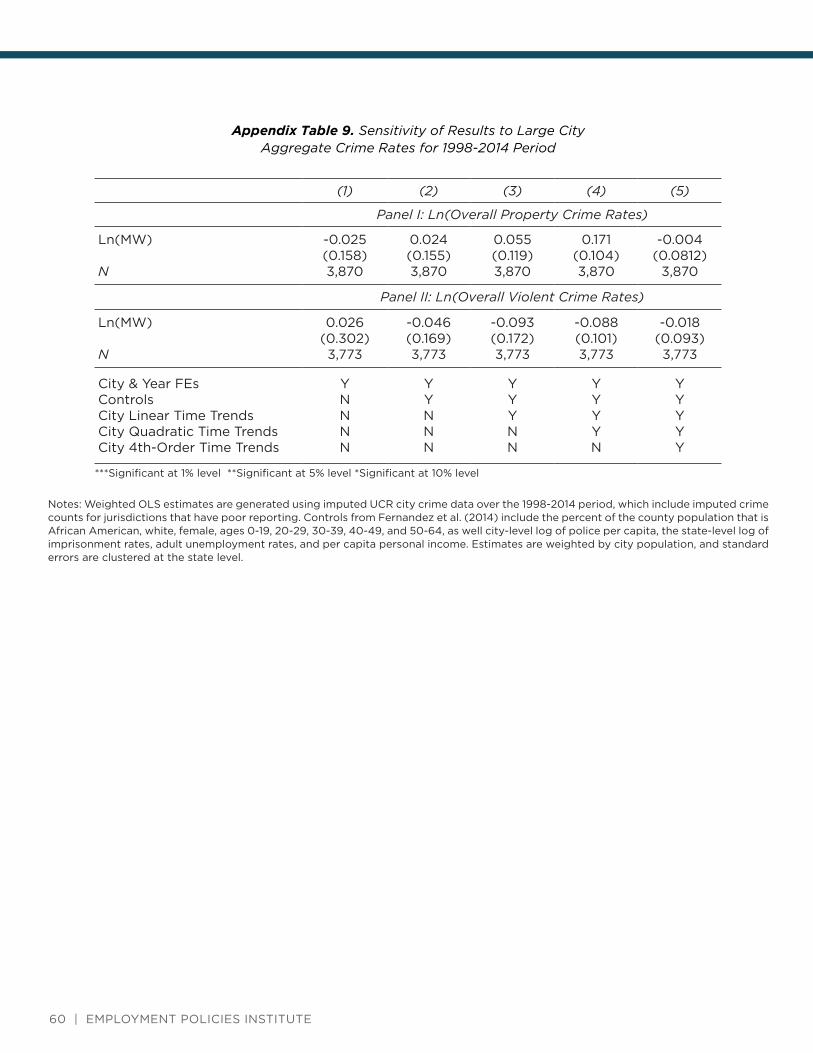
Appendix Table 9. Sensitivity of Results to Large City Aggregate Crime Rates for 1998-2014 Period


Notes: Weighted OLS estimates are generated using imputed UCR city crime data over the 1998-2014 period, which include imputed crime counts for jurisdictions that have poor reporting. Controls from Fernandez et al. (2014) include the percent of the county population that is African American, white, female, ages 0-19, 20-29, 30-39, 40-49, and 50-64, as well city-level log of police per capita, the state-level log of imprisonment rates, adult unemployment rates, and per capita personal income. Estimates are weighted by city population, and standard errors are clustered at the state level.

(1) (2) (3) (4) (5)

Panel I: Ln(Overall Property Crime Rates)

Ln(MW)

N

-0.025(0.158)3,870

0.024(0.155)3,870

0.055(0.119)3,870

0.171(0.104)3,870

-0.004(0.0812)

3,870

Panel II: Ln(Overall Violent Crime Rates)

Ln(MW)

N

0.026(0.302)3,773

-0.046(0.169)3,773

-0.093(0.172)3,773

-0.088(0.101)3,773

-0.018(0.093)3,773

City & Year FEs Controls City Linear Time TrendsCity Quadratic Time TrendsCity 4th-Order Time Trends

YNNNN

YYNNN

YYYNN

YYYYN

YYYYY


Appendix Table 10. Sensitivity of Estimated Relationship Between Minimum Wages and Crime Arrest Rates to Years included in the Sample, 16-to-24 year-olds, UCR, 2000-2016

Notes: Weighted OLS estimates are generated using data from the 2000-2016 Uniform Crime Reports. Arrest rates are arrests per 1,000 people of the specified age group. All regressions include controls for county fixed effects, year fixed effects, the number of agencies reporting to a county, county level percent male, African American, white, ages 0-19, 20-29, 30-39, 40-49, and 50-64, as well as state level police per capita, state level housing price index, the share of individuals with a college degree, an indicator for whether the governor is democrat, whether drug convicts are eligible for TANF benefits, whether parolees are eligible to vote, and the presence of a state EITC top-up. Samples are restricted to counties with crime arrest rates within two standard deviations of the county’s average crime arrest rate, and counties with a coverage indicator of at least 65%. Estimates are weighted by the county population of the specified age group. Standard errors are clustered at the state level.


(1) (2)


Ln(MW)

N

0.412(0.252)0.194

35,296

0.546***(0.201)0.269

40,347


Ln(MW)

ElasticityN

0.125(0.081)0.189

35,250

0.112(0.072)0.176

40,295


Ln(MW)

ElasticityN

0.471(0.368)0.216

35,374

0.228(0.332)0.109

40,422

YearsStates

2000-2014UCR States

2000-2016UCR States


EMPLOYMENT POLICIES INSTITUTE

NOTES

EPIONLINE.ORG

Do Minimum Wage Increases reduce crime?the National Incident Based Reporting System (NIBRS), and the...

Documents

Transcript of Do Minimum Wage Increases reduce crime?the National Incident Based Reporting System (NIBRS), and the...