Do Mature Economies Grow Exponentially?

Steffen Lange∗1, Peter Putz†2, and Thomas Kopp‡3

1Centre for Economic and Sociological Studies, Hamburg University;

Konzeptwerk Neue Okonomie, Leipzig2Centre for Statistics, Georg August University Gottingen

3Agricultural Market Analysis, Georg August University Gottingen

Abstract

Most models that try to explain economic growth indicate exponential

growth paths. In recent years, however, a lively discussion has emerged con-

sidering the validity of this notion. In the empirical literature dealing with

drivers of economic growth, the majority of articles is based upon an implicit

assumption of exponential growth. Few scholarly articles have addressed this

issue so far. In order to shed light on this issue, we estimate autoregressive

integrated moving average time series models based on Gross Domestic Prod-

uct Per Capita data for 18 mature economies from 1960 to 2013. We compare

the adequacy of linear and exponential growth models and conduct several

robustness checks. Our findings cast doubts on the widespread belief of expo-

nential growth and suggest a deeper discussion on alternative economic grow

theories.

Keywords: Gross Domestic Product Per Capita, exponential growth, linear growth,

time series analysis.

Acknowledgments:

Steffen Lange appreciates financial support from Hans Bockler Stiftung.

Thomas Kopp thanks Deutsche Forschungsgesellschaft (DFG) for funding through

Collaborative Research Centre 990.

∗s.lange@knoe.org†peter.puetz@uni-goettingen.de.‡thomas.kopp@agr.uni-goettingen.de (Corresponding author).

1

arX

iv:1

601.

0402

8v1

[q-

fin.

EC

] 1

5 Ja

n 20

16

Do Mature Economies Grow Exponentially?

1 Introduction

On November 2013, Lawrence Summer gave a seminal presentation at the annual

IMF Research Conference on policy responses to the current economic crises. At

this point, the great majority of economists studying the financial and the European

economic crisis shared the view, that economic growth needed to be reestablished

in order to solve the crisis. They solely disagreed upon the way to get there,

being divided into two camps the austerity versus Keynesian stimulus proponents.

Instead of arguing for either one of the two, Summers surprised his audience with

an innovative perspective on the debate. He argued, that the US economy has

entered secular stagnation - a new phase with constant low growth rates, and that

this situation was about to stay.

Summers is not the first to observe the persistently low growth rates though. Sev-

eral authors have, some already before the economic crises following 2007, argued

that growth rates are falling in mature economies, that is, economies that typ-

ically were part of the first wave of industrialization and have high per capita

incomes today. While most economists reason that high growth rates can and

should be regained (Reuter, 2000, p. 17), according to this diverging analysis the

low growth rates after the crisis are a continuation of decreasing growth rates for

several decades. In fact, it is argued that post-war growth in mature economies

depicts rather a linear than an exponential trend.

A significant number of authors argue that economic growth in early industrial-

ized, high-income countries depicts linear instead of exponential growth Afheldt

(1994); Altvater (2006); Bourcarde and Herzmann (2006); Glotzl; Reuter (2002);

Wegweiser et al. (2014); Hector Pollitt, Anthony Barker et al. (2004). These works

are to a large degree grey literature and to our knowledge particularly strong within

German-speaking debates. Even a subgroup of the German parliamentary commis-

sion on Growth, Welfare, Quality of Life expresses the view that macroeconomic

growth in Germany has depicted linear instead of exponential growth in the past:

Wie die Entwicklung des BIP in Deutschland in der Vergangenheit aber zeigt [...],

hat das BIP dauerhaft lediglich mit konstanten jhrlichen Zuwchsen zugenommen,

also linear statt exponentiell (p. 136). To our knowledge only two studies inves-

tigated this question empirically for a set of countries. Bourcarde and Herzmann

(2006) find linear growth for 15 and exponential growth for 5 countries out of a

sample of 20 countries. They look at macroeconomic growth instead of per capita

1

growth though and do not apply rigorous statistical methods. Wibe and Carlen

(2006) investigates the Gross Domestic Product Per Capita growth path of a total

of 28 countries and country aggregates. Their results indicate a linear growth in the

majority of the sample. We extend the work of Bourcarde and Herzmann (2006)

and Wibe and Carlen (2006) by using more recent data sets and more advanced

statistical tools.

The question, whether economic growth is exponential, depicts decreasing growth

rates or is of linear kind has important implications. First, it has serious implica-

tions for economic theory. The majority of economic (and in particular growth)

theories explicitly or implicitly assume exponential growth rates, as we see below.

If we observe linear growth, the theories and models need to be adjusted. Second,

various policies depend on the size of growth:

• Employment: If unemployment is the outcome of an interplay between produc-

tivity growth and economic growth Mankiw (2010), what labor policies are

needed in case of linear economic growth?

• Public debt: If calculations of the GDP to debt ratio and of debt repayments

are calculated based on predictions involving exponential growth rates, these

become unreliable in case of linear growth (Seidl and Zahrnt, 2010).

• Social security: The financing of social security systems is usually shaped ac-

cording to growth predictions based on exponential growth. In the situation

of linear growth the common projections of the financing of security systems

become unreliable and new strategies for long-term financing need to be de-

veloped (Chancel and Waisman, 2013).

• Environment: There are two opposing views on the relationship between eco-

nomic growth and environmental implications of economic activities. The

first argues for a Kuznets-Curve like relation. In growing economies, environ-

mental effects first increase and later decrease again (Grossman and Krueger,

1994). This view is increasingly repudiated though Stern et al. (1996); Dinda

(2004); Kaika and Zervas (2013). In the second view efficiency gains are not

correlated with economic growth (Stern, 2004). Therefore, economic growth

is associated with increasing environmental effects (Victor and Rosenbluth,

2007; Jackson, 2009; Kallis et al., 2012). In particular in the case of cli-

mate change, growth is argued to increase environmental effects Kaika and

Zervas (2013). Linear growth changes the calculations on the relationship

between economic growth and environmental impacts. This is likely to help

explain why decoupling seems to have taken place in certain countries re-

cently (Agency, 2014) and it changes the necessary efficiency gains needed,

2

which are usually calculated based on exponential growth Jackson (2009).

In this article we first examine prominent orthodox and heterodox economic growth

theories to what extend they do or do not predict exponential growth and why this

is the case (section 2), leading to the development of an exponential and a linear

growth function. The methods to test these functions empirically for 18 countries

from 1960-2013 are described in section 3. The corresponding results are presented

in section 4. Section 5 concludes.

2 Literature

2.1 Exponential growth as an inherent feature of modern growth

theories

Exponential economic growth is deeply routed within economic science and in par-

ticular within growth theories: Mainstream macroeconomic theory is profoundly

oriented towards an assumption of continuous, exponential GDP growth. Disrup-

tions in economic activity, such as expansions and recessions, are perceived as devi-

ations from the standard conception of a long-term stable macroeconomic growth

path (Pirgmaier et al., 2010, p. 1). The feature of exponential growth is part of

growth theories throughout the history of economic thought. In the following, we

give an overview of its role within several prominent schools of economic thought.

2.1.1 Early modern growth theories

After the classical contributions, which were very much engaged with growth the-

ory (although they termed it differently), economic growth became less prominent

in economics. Following the Great Recession in 1930 the topic became central

again. Harrod and Domar developed growth theories which entail concepts similar

to Keynes’ arguments at the time. Solow presented a first growth model in line

with neoclassical thought and his model became central for neoclassical growth

theory ever since.

Harrod

Harrod (1939) developed the concepts of warranted, actual and natural growth

rates. The warranted growth rate (gw) refers to the growth rate necessary for all

savings to be invested. The growth rate depends on the savings rate (s) and the

capital coefficient (v), as the later determines how much more can be produced per

3

unit of investments: gw = sv

1. The actual growth rate depends on the actual in-

vestments taking place. Assuming that all savings are equally used for investments,

the actual growth rate is given by

ga =s

va, (1)

with the actual increase in the capital coefficient va. The natural growth rate can

be regarded as an upper boundary of growth depending in particular on the labour

supply due to population growth and the work/leisure preference (Harrod, 1939,

p. 30). The central concept is in his own words: the geometric rate of growth of

income or output in the system, the increment being expressed as a fraction of its

existing level (Harrod, 1939, p. 16). All three kinds of growth are expressed as

growth rates.

The explanation lies within the setup of the model. Harrod builds his argument

on ratio parameters, most importantly the savings rate and the capital coefficient.

When savings are a percentage of production/income and investments need to

equal savings, investments grow exponentially. The same holds for the capital

coefficient: If the relation between capital and production increases by a certain

percentage each year, the capital intensity of the economy grows exponentially. As

a consequence, also production grows in an exponential manner.

Domar

The work by Domar (1946) constitutes the second pillar of modern growth theory.

In his approach, investments (I) on the one hand increase the capacity to produce

(dP ), dependent on the potential productivity of investments (σ) (Domar calls it

the potential social average investment productivity (Domar, 1946, p. 140)). This

is termed the capacity effect : dPdt = σI. On the other hand, investments increase

demand (dD). Its size depends on the size of investments and the savings rate, as

a lower savings rate imply a higher multiplier effect. This so-called demand effect

is given by: dDdt = dI

dt1s . Setting the two equal gives the condition that the growth

rate of investments (gI) needs to be equal to the product of the savings rate and

the potential productivity of investments:

gI = sσ. (2)

For Domars analysis the same holds as for Harrods: he builds his argument on ratio

parameters as the potential productivity of capital and the savings rate. Assum-

1The equations of this and the following sections are based on the respective articles referred

to.

4

ing a constant savings rate, exponential growth of investments is needed to make

use of savings. If the productivity of investments stays constant, this implies also

exponential economic growth.

Solow model

Solow (1956) developed, simultaneously to very similar work by Swan (1956), the

first neoclassical growth model. In this theory, the growth rate of the capital stock

( kk ) is determined by investments, which depend on savings (sF [k]) and the depre-

ciation of the capital stock (δk): kk = sF [k]

k −δ. In his model, the capital per worker

has decreasing marginal productivity. As the depreciation rate of the capital stock

does not change, capital accumulation comes to an end. This is not the case if tech-

nological change is included. Therefore, Solows model is extended by introducing

Harrod-neutral (i.e. labour-augmenting) technological change, which increases the

productivity of labor. It implies a growth of the effective labor, which leads to a

lower capital/labor ratio and subsequently increases the marginal productivity of

capital. Hence, investments become profitable again. In this scenario, the steady

state rate of economic growth is entirely determined by the speed of technological

change x (Barro and Sala-i martin, 2004):

g = x. (3)

Accordingly, the model produces exponential growth if a constant value for the

speed of technological change is assumed.

2.1.2 Neoclassical Growth Theories

Since Solow’s contributions, plenty of types and variations of neoclassical growth

models have been developed. In the following, the three most prominent types

are described. The neoclassical textbook model provides the microfoundations to

Solow’s model. The AK-model introduces constant returns to capital by including

human capital, and models with imperfect competition endogenize technological

change.

Neoclassical Textbook Growth Model

While Solow assumed a certain savings rate and a certain investment behavior of

firms, neoclassical growth models are based on the behavior of a representative

household and a representative firm. Households maximize utility due to a utility

function. Their savings depend on their preferences and the interest rate. Firms

maximize profits. They invest until the marginal productivity of capital is equal to

the real interest rate plus the rate of depreciation. Subsequently, in these models

5

savings and investments are brought into equilibrium via the interest rate (Barro

and Sala-i martin, 2004, Chapter 2).

The equilibrium growth rate of the capital stock is similar to the Solow-model.

The change in the capital stock is determined by the difference between output

and consumption. Additionally, the capital needed for depreciation and due to

technological change is subtracted:˙kk = f(k)−c

k− (δ + x).

The growth of per capita income (g) depends - as in the Solow model primarily on

the rate of technological progress (x) though: the steady-state per capita growth

rate equals the rate of technological progress, x, which is assumed to be exogenous

(Barro and Sala-i martin, 2004, p. 205). Also, A greater willingness to save or an

improvement in the level of technology shows up in the long run as higher levels of

capital and output per effective worker but in no change in the per capita growth

rate (p. 210):

g = x. (4)

The neoclassical textbook model therefore leads to the same conclusion concerning

exponential growth as did the Solow-model: As long as technological change is

assumed to be of a constant rate, economic growth is exponential.

Endogenous growth I: The AK-model

The unsatisfactory result from neoclassical growth theories, that economic growth

depends purely on an exogenously given rate of technological progress in the neo-

classical growth theories motivated the development of models which explain con-

tinuous growth differently. In the AK-model capital has constant instead of dimin-

ishing marginal returns, due to the fact that capital is understood in broader terms,

including human capital. Production in this model depends on the technological

state (a) and the amount of capital (k): y = ak. Growth of capital per capita

( kk ) and income per capita ( yy or g) depend, without technological change, on the

size of net investments which depend on the savings rate and the depreciation rate

(Barro and Sala-i martin, 2004, Chapter 1 and 4):

g =y

y=k

k= sA− δ (5)

The AK-model is therefore also designed to depict exponential growth. The reason

lies within the ratio of the savings rate that determines capital accumulation with

constant returns. Thereby investments grow exponentially and so does per capita

6

income.

Endogenous growth II: Imperfect competition

Endogenous growth models with imperfect competition assume markets (of monop-

olistic competition) (Aghion et al., 1998) in which firms invest into new production

methods or the improvements of the existing methods because they have a tem-

porary patent on the new method which allows them to make profits. The rate of

technological change and hence the rate of economic growth depends on how fast

new intermediate goods are invented. This is determined by several factors. First,

the preferences of households concerning consumption and savings (θ represents

the households willingnesses to have different consumption levels over time and ρ

stands for the time preference of the households) influence the amount of resources

put into developing new technologies. A second set of parameters influence the

speed of technological change: The price of inventing new technologies (η) and the

size of the mark-up (α) a firm can put on the new technology. Finally, the state

of technology (A) and the amount of the labor employed (L) influence the growth

rate. The following equation gives an example of the determinants of economic

growth (Barro and Sala-i martin, 2004, Chapter 6 and 7):

Y

Y=

1

θ[L

ηA

11−α (

1 − α

α)α

21−α − ρ]. (6)

Here, growth is also represented as a rate (this time it is not per capita growth

but macroeconomic growth). A change in each of the factors mentioned therefore

alters the rate of growth. Again, constant parameters lead to exponential growth

in this model.

2.1.3 Heterodox growth theories

In neoclassical frameworks growth depends on two central aspects: savings lead

to investments and technological change increases labor productivity. Heterodox

growth theories also regard these factors as central, but analyze the underlying

mechanisms very differently. Generally speaking, investments are not only deter-

mined by savings but also other factors and technological change either depends

on investments or is the effect of market competition.

Marxian

In Marx’s theory, firms buy labor (variable capital), materials and physical capital

(constant capital) in order to manufacture products that they sell on a competi-

tive market. Firms can make profits due to the exploitation of labor, i.e. because

7

workers are paid due to their cost of reproduction that usually is below the value

of their labor power (Harvey, 2006). As firms sell their products on a competitive

market they are forced to invest their profits into new production technologies. In

case they do not so, they are outcompeted by their rivals who did and therefore

are able to offer products at a lower price (Mandel, 1969). The degree of competi-

tion is the prime determinant of the share of profits (a) reinvested (a = Iπ ). The

profit rate (r) is primarily due to the bargaining process between capital and labor

(r = πK ). The growth rate of the capital stock, which is equivalent to the growth

rate of output (g) depends on these two factors (Hein, 2002):

g =I

K= ar. (7)

Investments go hand in hand with technological change. The introduction of new

technologies changes the organic composition of capital. It increases the ratio be-

tween constant and variable capital. Investments hence have ambiguous effects on

employment. On the one hand they increase the demand for labor, as production

increases. On the other hand, the labor-coefficient decreases, which decreases the

demand for labor. Marx argues, that the second mechanism guarantees a continu-

ous existence of a ’reserve army’, i.e. a continuous availability of workers.

Whether the Marxian theory suggests an exponential growth pattern or not is up to

constant debate. It is disputed under the term Tendency of the rate of profit to fall.

On the one hand it is argued, that the change in the organic composition of capital

decreases the profit rate. The intuitive reason is, that surplus is generated due

to the exploitation of labor power. Therefore, assuming everything else constant,

using relatively less labor in the production process also implies less possibility

to generate surplus and profits. On the other hand, if the surplus rate (the ratio

between surplus and variable capital) increases, this tendency can be countervailed

(Sweezy, 1943). Hence, the Marxian analysis leaves it open, whether economic

growth takes place at a certain rate (and hence is exonential) or whether the growth

rate declines.

Kalecki

Kalecki et al. (1987) developed a growth theory that builds on both Marxian and

Keynesian analyses and concepts. Investments are at the center of his argument.

The economy is divided into three sectors which produce (1) capital goods for

investments (I), (2) consumption goods for capitalists (CK) and (3) consumption

goods for workers (CW ). The size of the economy Y is therefore given by Y = I +

CK+CW . In each sector capitalists earn profits (P ) and workers earn wages (W ).

There are no savings out of wages. Investments and the consumption of capitalists

8

determine profits: P = I +CK. Investments determine growth. Its effect depends

on the wage share (w) and the consumption rate of profits (q):∆Y = ∆I(1−w)(1−q) .

According to Kalecki et al. (1987) there are five central determinants of investments.

(1) Firms savings (S) induce entrepreneurs to invest more, as they have more fi-

nancial means. (2) An increase (decrease) in firms profits ∆P∆t stimulate (attenuate)

them to increase investments because production has become more profitable. (3)

A change in the capital stock ∆K∆t increases/decreases investments because addi-

tional profits due to investments are lower/higher for a higher/lower level of existing

capital. (4) An increase in production in the past ∆Y∆t induces investments because

inventories are proportionate to production. (5) Finally, investments may change

due to various long run changes (d) in the economy (technological change, interest

rate, company share earnings): It+1 = aSt + b∆P∆t − c∆K

∆t + e∆Y∆t + d.

Kalecki further argues, that the change in profits, the change of the capital stock

and the change in production all primarily depend on the investments of the past.

Subsequently, investments are a function of past investments, several behavioral

parameters (covered by a, b, c, e, q, p) and the long-term changes (d): It+1 = aIt −c∆K

∆t + 11−q (b+ e

1−w )∆I∆t + d

Investments are the sum of a fraction of the past investment level (aIt), the change

of investments in the past multiplied by some constant ( 11−q (b+ e

1−w )∆I∆t ) and the

change of the capital stock multiplied by some constant (c∆K∆t ). Assuming constant

behavioral parameters, economic growth in Kaleckis theory therefore tends to also

be exponential. This can best be illustrated by assuming that a = 1 and abstracting

from depreciation of the capital stock. Defining f = 11−q (b+ e

1−w ), we get

It+1 = It + (f − c)∆I

∆t. (8)

As long as f > c, the growth of investments is therefore of exponential nature.

Assuming a constant capital coefficient and constant population, economic growth

is therefore also exponential. The result can only be different, if the parameters

change over time.

The standard Keynesian growth model

(Hein, 2004, chapter 7) develops a standard Keynesian model of growth and dis-

tribution. In this model there are only savings out of profits, so the savings rate

(savings/capital stock, s) is equal to the savings ratio out of profits (sπ) multiplied

by the profit rate (profits/capital stock, r): s = sπr. The growth rate of the capital

stock is firstly determined by animal spirits (α) (e.g. (Fontana and Sawyer, 2015))

and, secondly, by the investment reaction (β) to the profit rate (r): g = α + βr

9

(e.g. Kalecki et al. (1987)). A steady-state growth rate exists, where the growth

rate (g) is equal to the savings rate: g = s. Combining these equations one gets

the equilibrium growth rate

g = s =sπα

sπ − β(9)

In this case, the growth rate stays constant, if the other parameters also stay

constant. Again the model depicts exponential growth.

2.2 Explanations for diminishing growth rates

Discussions on an end to economic growth have existed at least since the beginning

of modern economic theory. All the major classical economists had a concept of

the steady-state, that marked an end to economic expansion (Luks, 2001). The

term secular stagnation was coined by (Hansen, 1939) in the Great Depression. He

argued that a limit to geographical expansion, seizing population growth and less

capital-intensive technologies resulted in lower investment rates and lower growth.

In the first controversy on this issue, Schumpeter (1939) on the other hand argued

that unfavorable business conditions for entrepreneurs were the reason for lacking

growth rates. While this first discussion was ended by World War Two and the

economic expansion of Western Europe and Northern America afterwards, it came

up again with the stagflation in the 1970s. Sweezy (1982) argued, that again

the lack of investments was the reason that, while recovery of a growth path was

possible in theory, nothing like that is visible on the horizon now (Sweezy, 1982,

p. 9). The discussion has been taken up again after the global financial crisis after

2007 and has gained momentum after the speech by Summers mentioned in the

beginning of this article. However, there are also arguments for declining and/or

linear growth which are not associated to the term secular stagnation. In the

following several different reasonings, which mostly also refer to one or several of

the theoretical frameworks developed in section 2, are discussed.

2.2.1 Slower technological change

As we have seen above, technology plays a central role in explaining economic

growth. Hence, it is not surprising that some authors see slower technological

change as being the reason for declining growth rates. It is argued, that the tech-

nological progress in recent decades has increased labor productivity less than in

the decades before and that it is the nature of the technological change that is the

explanatory of less growth. Gordon (2012) argues that capitalism has experienced

10

three industrial revolutions (IR): ”The first (IR #1) with its main inventions be-

tween 1750 and 1830 created steam engines, cotton spinning, and railroads. The

second (IR #2) was the most important, with its three central inventions of elec-

tricity, the internal combustion engine, and running water with indoor plumbing, in

the relatively short interval of 1870 to 1900. [...] The computer and Internet revo-

lution (IR #3) began around 1960 and reached its climax in the dot.com era of the

late 1990s“ (Gordon, 2012, p. 1-2). For him the divergent impacts of the innova-

tions on labor productivity explain different growth rates. Much of the high growth

rates in the 1950s to 1970s can be explained by a combination of applications of

technologies from the second and third industrial revolution. Since 1972 the effects

of the implication of technologies from the second industrial revolution have faded

out and the remaining effects of the third revolution are a major explanation for the

low growth rates that we observe today in mature economies(Gordon, 2014a). This

analysis directly refers to the early growth theories with exogenous technological

growth. While Gordon takes into account that the speed of technological change

is also influenced by other factors, he argues for a baseline rate of technological

change Gordon (2014b). This baseline is exogenously given.

2.2.2 Labor and human capital

Within the recent discussion on secular stagnation there are two arguments con-

cerning labor. First, the average number of working hours per capita has decreased

and is predicted to continue to do so in the future. While the average working hours

per worker have declined in Europe (not so much in Northern America), the par-

ticipation rate of women has increased Maddison (2006). As someone also has to

do the reproductive work, this leaves little room for an extension of labor hours

in the future (Netzwerk Vorsorgendes Wirtschaften, 2013). The major reason for

declining average working hours is the demographic change though, leading to an

increase in the dependency ratio. This is anticipated to continue in the future for

almost all countries investigated in this paper. Based on these findings, Johansson

and Guillemette (2012) come to the conclusion that ’Population ageing, due to

the decline in fertility rates and generalized gains in longevity, has a potentially

negative effect on trend growth as it leads to a declining share of the working age

population as currently defined (15-64 years)‘ (Johansson and Guillemette, 2012,

p. 13). Second, it is argued that the advantages from education to increase the

productivity of workers have declined over the past decades and that this trend is

likely to continue. Gordon (2014b) see the major reasons in certain institutions.

They argue, that future increases in high school completion rates are prevented

11

by dropping out, especially of minority students (p. 51) and that the inability for

many to finance academic studies is a major problem to further improve education.

Similarly, Eichengreen (2014) argues that the US government has spend too little

on public education over the past decades. The second argument relates to the

views of endogenous growth theories including the role of human capital. From

this perspective, the investments into human capital have been low, so that growth

is also low. Another explanation could be, that marginal returns to human capital

are diminishing. To our knowledge, this argument has not been made yet though.

2.2.3 Insufficient investments

Investments play a crucial role for economic growth, as was the case in all growth

theories covered above. They are important for capital deepening and the applica-

tion of new technologies. Within the recent literature on secular stagnation, several

reasons for insufficient investments have been pointed at: (1) Eichengreen (2014)

argues that low investments by the government, in particular in infrastructure, have

been a major reason for overall low investments in the USA. (2) The decrease in

population growth decreases overall investments and therefore slows down the ap-

plication of new technologies hence dampens technological change (Hansen, 1939;

Krugman, 2014). (3) It is argued that working aged people buy relatively more

capital-intensive goods (in particular housing) and that the demographic change

has therefore decreased the demand for such goods, which also dampens overall

investments (Hansen, 1939; Krugman, 2014). The causes of low investments are

hence argued to be found in low demand or low governmental investments. Accord-

ingly, these views refer to the heterodox and in particular the Keynesian theories

on growth.

2.2.4 Non-competitive market structures

Another explanation for decreasing investment rates refers to market structures.

This work builds on marxian reasoning as outlined above. While Marx assumed

perfect competition in that argument, Baran and Sweezy (1966) argue that post-

war capitalism was marked by increasing concentration of market power. There-

fore oligopolistic and monopolistic market structures had become the dominant

form of market structures. Steindl (1976) argues that such structures introduce

several mechanisms which overall lower investment and growth rates. The mono-

/oligopolistic structures increase profit rates within the concentrated sectors and

thereby lower aggregate demand (assuming higher savings out of profits than out of

12

wages). At the same time, investments in these sectors are as monopolists maximize

profits with investments and production below the level within competitive mar-

kets. Due to the low demand, other profitable investment opportunities are scarce

though, leading to an overall reduced level of investments and an equilibrium be-

low potential output. Foster (2014) comes to the conclusion that the outcome of

concentrated markets is ’a chronic condition of secular stagnation’ Foster (2014, p.

87).

2.2.5 Consumption demand

Consumption is the second major component of aggregate demand. Next to invest-

ments, a slow increase in consumption can therefore be another major cause for low

growth. There are again two central arguments. Within the discourse on secular

stagnation, it is argued that consumption slackens due to high income and wealth

inequalities and the accompanying household debts. Summers (2014b) point out

that changes in the distribution of income, both between labor income and capital

income and between those with more wealth and those with less, have operated to

raise the propensity to save, as have increases in corporate-retained earnings (p.

69). Summers argues that this is a reason for the decline of the interest rate. It

also decreases consumption though: Rising inequality operates to raise the share

of income going to those with a lower propensity to spend (Summers, 2014a, p.

33). Krugman (2011) argues on the other hand, that at least before the crisis, the

reason for low growth was not high savings (as the savings rate was not high) but

the trade-deficit in the USA . Nevertheless, Summers’ argument that is also being

made by other such as Gordon (2014b) and Eggertsson and Mehrotra (2014) can

be maintained when looking at other countries of our sample. The second argu-

ment refers not to a lower propensity to consume for higher income-earners at a

certain point in time but over time. The argument is, that due to several mech-

anisms, with increasing average income, people consume a lower share of their

income. This leads to only slowly increasing aggregate demand and subsequently

to low growth. Reuter (2000) made this argument long before the global financial

crisis. He argues that the satisfaction of needs combined with institutional limits

to exponentially increasing consumption are responsible for only slowly increasing

consumption and slow growth. In fact, this line of argument goes back to Keynes’

work. Keynes (1933) argued that with increasing average income, people would

choose leisure time over further consumption increases. These lines of argument

therefore directly correspond to the Keynesian growth theories discussed above.

13

2.2.6 Slower increase in energy use

In most economic growth theories, the environment is either seen as a source for

natural resources and/or a sink for emissions. Accordingly, the use of natural

resources is mostly modeled as a third input into the production function. In neo-

classical theory and environmental economics, natural resources are assumed to

be substitutable by physical capital. In ecological economics on the other hand,

substitution between them is regarded to be very limited as they are primarily com-

plements. Based on this analysis, several authors have argued that by accounting

for exergy and/or useful work, economic growth can be accounted for to a much

higher degree than by traditional procedures. Ayres and Warr (2005) find that

useful work can explain much of past economic growth. Interestingly, they can

explain the growth until the mid-1970s almost entirely, while afterwards, this is

less the case. From this point in history, the increase of useful work slows down

significantly. Economic growth slows down less so. An interpretation could be,

that the increase in energy prices has led to a new technological trajectory, which

is depicted by less use of energy and at the same time less productivity growth. At

the same time, there are many other changes going on and this phenomenon needs

further investigation.

3 Methods and Data

As we have seen, most prominent growth theories argue for an exponential growth

pattern. This is represented by one or several ratios, be it the savings ratio, the

speed of technological change, the profit rate or the potential productivity of in-

vestments. Accordingly, a Gross Domestic Product Per Capita (GDPPC) series

underlying the growth models covered so far (excluding the Marxian theory, which

is not clear in this respect) can be represented within a simple regression framework

by the following term:

GDPPCt = b0bt1 + εt = b0 (1 + r)t + εt, t = 0, . . . , T − 1, (10)

where b0 denotes the starting value in t = 0 of the series with T observations, b1

(and thus r) determines the growth of the series, and εt is the error term for the

observation in t.

As an alternative hypothesis we test the exponential model against the simplest

model of diminishing growth rates, which is a model of linear growth:

14

GDPPCt = b0 + b1t+ εt = b0 + (1 + r) t+ εt, t = 0, . . . , T − 1, (11)

where b1 (and thus r) now enters the equation in a linear fashion which corresponds

to a constant increase of the GDPPC .

In order to examine these growth theories on an empirical basis, we look at the

economic development for a set of 18 mature economies from 1960 to 2013. In

particular, we decided for investigating yearly real GDPPC series for the group

of Western and Southern European countries and Western offshoots (as defined

by Maddison (2006, Appendix B)). Germany was left out of the sample in order

to avoid problems of aggregation during the period before re-unification in 1990.

Luxembourg was added, which Maddison includes in the group of Small West

European Countries (Maddison, 2006, p. 179). A full overview of the selected

countries can be found below in table 1. The rationale behind the starting point

in 1960 is that effects of World War Two should have vanished by then. As Crafts

and Toniolo (1996) argue, ’In five years at most, Europe recovered the ground lost

relative to the highest prewar income levels. It is, thus, quite safe to place the end

of the first phase of reconstruction and the beginning of a new era in the history of

European economic growth in 1950.’ (Crafts and Toniolo, 1996, p. 3). Since the

data is only available since 1960, we start from there.

It has been argued that the second major reason for high growth rates in Eu-

rope (including the majority of countries of our sample) after World War Two was

convergence. The US-American economy had introduced new production meth-

ods characterised by higher labour productivities over the previous decades, which

European countries had not. From the end of World War Two until the end of

the 1960s the introduction of such technologies in European countries facilitated

the high growth rates (Eichengreen, 2008). In order to exclude this effect, we

additionally execute the empirical investigation for the period 1970-2013.

Due to partly differing GDPPC measures, we analyse two data sets: World Bank

GDPPC series in US$ with 2005 prices and Conference Board GDPPC series in

US$ with 2014 prices. Since the results are very similar, we only report the results

for the first data set mentioned above.2 In this data set, GDPPC data for New

Zealand and Switzerland are only available from 1970-2013.

In a preliminary analysis we compare for each country the coefficients of determina-

tion R2 between a regression of the GDPPC series on a linear and on an exponential

2The data sets, non-reported results and the software code can be obtained from the authors

upon request.

15

time trend.3 The first regression corresponds to equation (11) and the latter to

equation (10). In order to obtain the optimal exponential growth rate within the

regression framework, the exponential growth model is estimated for a grid over 50

equidistant values between 0 and 0.06 for r4 and the highest R2 is selected.

This procedure represents a rather descriptive approach of comparing linear and

exponential growth of the GDPPC . Making credible quantitative statements about

the data generating process behind the time series is, however, only valid for sta-

tionary series. Only after taking account for possible unit roots and autocorrelation

of time series it is reasonable to compare the adequacy (in terms of predictive abil-

ity) between different time series models. Note that these issues were not tackled

by Wibe and Carlen (2006) and Bourcarde and Herzmann (2006). We therefore

apply the Box-Jenkins method (Box et al., 2011) to find suitable models for the

series at hand. The first step is to determine the order of integration of the time

series. Initialised by Nelson and Plosser (1982), there has been an extensive debate

on whether macroeconomic time series are trend-stationary or follow a unit root

process with a potential drift, see for instance Perron (1989), Shin et al. (1992)

and Cuestas and Garratt (2011). The latter view seems to be the more prominent

in the literature as most authors apply unit root and co-integration techniques to

macroeconomic time series like the GDPPC. In order to check whether unit root

methods are also required for the data set at hand, we conduct for each country

the augmented Dickey-Fuller test for both the original time series and the loga-

rithm (log) of GDPPC series after removing their linear time trends. Note that

removing a linear time trend from a log-transformed time series corresponds to

the deletion of an exponential time trend of the original series. A rejection of the

null hypothesis suggests the absence of a unit root and therefore trend-stationarity.

Likewise, we conduct the KPSS test for the same series, yet the null hypothesis

for this test is trend-stationarity. The results of these tests can be found in Ta-

ble 5 in the appendix. As we find no strong evidence against a unit root and for

trend-stationarity in both the original and the log transformed GDPPC in any of

the countries except for Switzerland,5 we generally assume the series to follow unit

root processes with drift terms. We are aware of the heterogeneity of the countries

and the weaknesses of the underlying tests, as pointed out in Cuestas and Garratt

(2011). In particular, our simple time trend models might not capture true non-

3Note that this approach is essentially equivalent to the comparison of the log-likelihood be-

tween a non-transformed and a log-transformed GDPPC series as done by Wibe and Carlen (2006)

who used GDPPC data up to 2005.4Clearly, all countries in our sample exhibit a positive growth within the time frame under

consideration.5We chose a significance level of 5%.

16

linear patterns, for instance caused by structural breaks. Nevertheless, as our test

results are quite unambiguous, we are confident that the aggregate findings of the

following analysis should be credible.

Assuming a unit root, the next step is to determine the orders p and q of the

autoregressive process and the moving average process in a suitable ARIMA (p, 1, q)

model with drift. In order to do so, we use the auto.arima function of the R package

forecast (Hyndman and Khandakar, 2008). More specific, we choose among all

candidate models with maximum lag orders p = q = 3 the most appropriate one

with respect to the Akaike Information Criterion for finite sample sizes (AICc).6

This procedure achieves an appropriate compromise between a lack-of-fit to the

data and a too complex model. As we are estimating an ARIMA(p, 1, q) with drift,

we actually model the first differences of GDPPC series. Allowing for a potential

exponential growth, this leads in the simplest case with p = q = 0 to the model

∆GDPPCt = GDPPCt−GDPPCt−1 = b0 (1 + r)t−1 + εt, t = 1, . . . , T − 1 (12)

where the errors εt are assumed to be independent and identically distributed and b0

describes the difference between the first two observations which grows over time at

the rate r. A constant and thus linear growth is given for r = 0. We exploit exactly

this property to decide for either a linear or an exponential growth model by using a

similar approach as above: first, for each of the 50 equidistant values between 0 and

0.06 for r, the most suitable ARIMA (p, 1, q) model with drift with respect to the

AICc is chosen. In a second step we decide for the final model with a corresponding

growth rate (which we subsequently refer to as optimal model with optimal growth

rate) by comparing the value of several selection criteria amongst all 50 ARIMA

(p, 1, q) models chosen in the first step. The predictive ability of different time

series models is often compared by the accuracy of pseudo-out-of-sample-forecasts.

In those cases, the particular models are fitted to a subsample of the data (e.g. all

observations except for the last 5 years) and the last data points are predicted based

on the estimated model parameters. This procedure essentially tells us which model

forecasts better at the end of the sample. However, we are aware of a potentially big

influence of the recent financial crisis on the results if we solely compared forecast

accuracy for the last years. Thus, for our second step of final model selection, we use

the Akaike Information Criterion (AIC), which includes all observed data points

and can thus be seen as a measure for predictive ability for the whole sample

6We also use the Bayesian Information Criterion (BIC) for model selection in this step and

obtained very similar results. For a comprehensive discussion on model selection criteria in time

series models, see Hyndman et al. (2008, chap. 7).

17

(Hyndman et al., 2008, chap. 7). Furthermore, we also base our selection of

the optimal model on the AICc and the more parsimonious Bayesian Information

Criterion (BIC). Despite the advantages of such model selection criteria, the results

are still likely to depend on the chosen sample. For this reason we repeat the

analysis with excluding the recent financial crisis, i.e. considering only the years

1960-2007. As a further robustness check, we discard the first 10 years of the

sampling period and thereby restrict our analysis to the years 1970-2013, in order

to exclude the effect of convergence, as argued above.

4 Results

The results of the R2 comparison between the best exponential fit (chosen among

all 50 grid values for the growth rate r) and the linear fit can be found in table

1. For the majority of countries, the linear model fits the data more accurately

than the exponential one. In a couple of countries, the evidence points into the

opposite direction, with the differences between the models being rather small in

these cases, however.

Table 2 depicts the optimal growth rate of the optimal ARIMA (p, 1, q) model

(with respect to the model selection criteria AIC, AICc and BIC after our two-step

selection procedure) explaining the observed GDPPC series for each country.

The linear growth model with r = 0 is preferred for 11 out of 18 countries with

respect to the AIC. Note that some optimal growth rates are not equal but close to

zero and thus far from the magnitude that is usually talked about when discussing

growth rates, indicating a quasi-linear growth. Such an example is Sweden which

exhibits an optimal growth rate of only 0.25%. The behaviour of the AIC over all

grid values for the growth rate r is shown in Figure 1 for the case of Sweden. It can

be seen that the lowest AIC at the growth rate 0.25% is very close to the AIC for

the linear model with r = 0, whereas it becomes considerably larger for increasing

values of r.7

The results are fairly robust for the chosen model selection criteria, with the only

exception being Italy: here, the AIC and AICc indicate an exponential growth

model with the largest growth rate r = 0.06 on our grid, whereas the BIC prefers

the linear model. A closer look at the optimal ARIMA(1, 1, 3) model chosen by

AIC and AICc shows a near unit root autoregressive coefficient of 0.9989 and

7Naturally, a quantitative comparison between a linear and an exponential growth model for a

single country is in general not possible if the linear model is chosen, since there is no comparable

best exponential growth model.

18

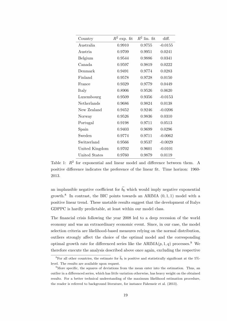
Country R2 exp. fit R2 lin. fit diff.

Australia 0.9910 0.9755 -0.0155

Austria 0.9709 0.9951 0.0241

Belgium 0.9544 0.9886 0.0341

Canada 0.9597 0.9819 0.0222

Denmark 0.9491 0.9774 0.0283

Finland 0.9578 0.9728 0.0150

France 0.9329 0.9779 0.0449

Italy 0.8906 0.9526 0.0620

Luxembourg 0.9509 0.9356 -0.0153

Netherlands 0.9686 0.9824 0.0138

New Zealand 0.9452 0.9246 -0.0206

Norway 0.9526 0.9836 0.0310

Portugal 0.9198 0.9711 0.0513

Spain 0.9403 0.9699 0.0296

Sweden 0.9774 0.9711 -0.0062

Switzerland 0.9566 0.9537 -0.0029

United Kingdom 0.9702 0.9601 -0.0101

United States 0.9760 0.9879 0.0119

Table 1: R2 for exponential and linear model and difference between them. A

positive difference indicates the preference of the linear fit. Time horizon: 1960-

2013.

an implausible negative coefficient for b0 which would imply negative exponential

growth.8 In contrast, the BIC points towards an ARIMA (0, 1, 1) model with a

positive linear trend. These unstable results suggest that the development of Italys

GDPPC is hardly predictable, at least within our model class.

The financial crisis following the year 2008 led to a deep recession of the world

economy and was an extraordinary economic event. Since, in our case, the model

selection criteria are likelihood-based measures relying on the normal distribution,

outliers strongly affect the choice of the optimal model and the corresponding

optimal growth rate for differenced series like the ARIMA(p, 1, q) processes.9 We

therefore execute the analysis described above once again, excluding the respective

8For all other countries, the estimate for b0 is positive and statistically significant at the 5%-

level. The results are available upon request.9More specific, the squares of deviations from the mean enter into the estimation. Thus, an

outlier in a differenced series, which has little variation otherwise, has heavy weight on the obtained

results. For a better technical understanding of the maximum likelihood estimation procedure,

the reader is referred to background literature, for instance Fahrmeir et al. (2013).

19

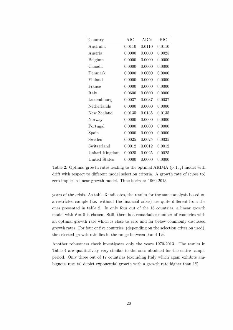
Country AIC AICc BIC

Australia 0.0110 0.0110 0.0110

Austria 0.0000 0.0000 0.0025

Belgium 0.0000 0.0000 0.0000

Canada 0.0000 0.0000 0.0000

Denmark 0.0000 0.0000 0.0000

Finland 0.0000 0.0000 0.0000

France 0.0000 0.0000 0.0000

Italy 0.0600 0.0600 0.0000

Luxembourg 0.0037 0.0037 0.0037

Netherlands 0.0000 0.0000 0.0000

New Zealand 0.0135 0.0135 0.0135

Norway 0.0000 0.0000 0.0000

Portugal 0.0000 0.0000 0.0000

Spain 0.0000 0.0000 0.0000

Sweden 0.0025 0.0025 0.0025

Switzerland 0.0012 0.0012 0.0012

United Kingdom 0.0025 0.0025 0.0025

United States 0.0000 0.0000 0.0000

Table 2: Optimal growth rates leading to the optimal ARIMA (p, 1, q) model with

drift with respect to different model selection criteria. A growth rate of (close to)

zero implies a linear growth model. Time horizon: 1960-2013.

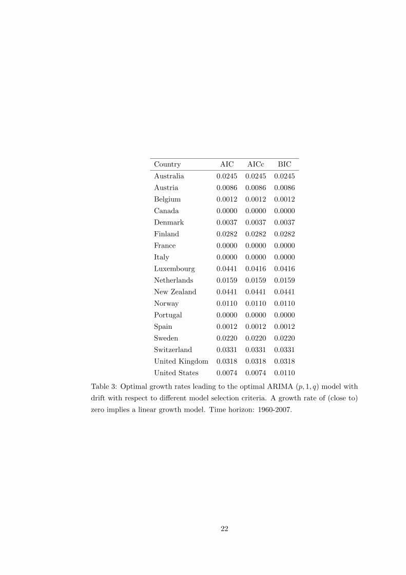
years of the crisis. As table 3 indicates, the results for the same analysis based on

a restricted sample (i.e. without the financial crisis) are quite different from the

ones presented in table 2. In only four out of the 18 countries, a linear growth

model with r = 0 is chosen. Still, there is a remarkable number of countries with

an optimal growth rate which is close to zero and far below commonly discussed

growth rates: For four or five countries, (depending on the selection criterion used),

the selected growth rate lies in the range between 0 and 1%.

Another robustness check investigates only the years 1970-2013. The results in

Table 4 are qualitatively very similar to the ones obtained for the entire sample

period. Only three out of 17 countries (excluding Italy which again exhibits am-

biguous results) depict exponential growth with a growth rate higher than 1%.

20

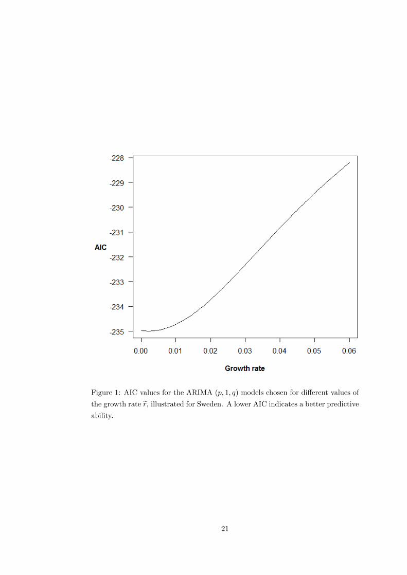
Figure 1: AIC values for the ARIMA (p, 1, q) models chosen for different values of

the growth rate r, illustrated for Sweden. A lower AIC indicates a better predictive

ability.

21

Country AIC AICc BIC

Australia 0.0245 0.0245 0.0245

Austria 0.0086 0.0086 0.0086

Belgium 0.0012 0.0012 0.0012

Canada 0.0000 0.0000 0.0000

Denmark 0.0037 0.0037 0.0037

Finland 0.0282 0.0282 0.0282

France 0.0000 0.0000 0.0000

Italy 0.0000 0.0000 0.0000

Luxembourg 0.0441 0.0416 0.0416

Netherlands 0.0159 0.0159 0.0159

New Zealand 0.0441 0.0441 0.0441

Norway 0.0110 0.0110 0.0110

Portugal 0.0000 0.0000 0.0000

Spain 0.0012 0.0012 0.0012

Sweden 0.0220 0.0220 0.0220

Switzerland 0.0331 0.0331 0.0331

United Kingdom 0.0318 0.0318 0.0318

United States 0.0074 0.0074 0.0110

Table 3: Optimal growth rates leading to the optimal ARIMA (p, 1, q) model with

drift with respect to different model selection criteria. A growth rate of (close to)

zero implies a linear growth model. Time horizon: 1960-2007.

22

Country AIC AICc BIC

Australia 0.0172 0.0172 0.0172

Austria 0.0000 0.0000 0.0000

Belgium 0.0000 0.0000 0.0000

Canada 0.0000 0.0000 0.0000

Denmark 0.0000 0.0000 0.0000

Finland 0.0000 0.0000 0.0000

France 0.0000 0.0000 0.0000

Italy 0.0551 0.0000 0.0000

Luxembourg 0.0000 0.0000 0.0000

Netherlands 0.0000 0.0000 0.0000

New Zealand 0.0135 0.0135 0.0135

Norway 0.0000 0.0000 0.0000

Portugal 0.0000 0.0000 0.0000

Spain 0.0000 0.0000 0.0000

Sweden 0.0233 0.0135 0.0135

Switzerland 0.0012 0.0012 0.0012

United Kingdom 0.0000 0.0000 0.0000

United States 0.0000 0.0000 0.0000

Table 4: Optimal growth rates leading to the optimal ARIMA (p, 1, q) model with

drift with respect to different model selection criteria. A growth rate of (close to)

zero implies a linear growth model. Time horizon: 1970-2013.

23

5 Conclusion

The overall picture of our analyses casts doubts on the widespread belief of expo-

nential growth. The results are not distinct in the sense that we could find clear

evidence whether growth in economically developed countries is in general expo-

nential or linear. We observe, however, high dependence on the sample period, in

particular on the inclusion of the recent crisis (2008-2013). Besides, our modelling

approach is somehow restricted as we only consider linear and exponential trends

in ARIMA (p, 1, q) models. For some of our selected countries other models might

reflect the development of their yearly GDPPC more accurately. With regard to

these caveats, we do not want to overreach in the interpretation of our results. Nev-

ertheless, while using more appropriate time series models and more recent data,

our main finding is in line with Wibe and Carlen (2006) and Bourcarde and Herz-

mann (2006): In contrast to the prominent view of exponential economic growth, a

constant growth might be closer to the truth of what has happened in some mature

economies within the last 40-50 years .

References

Afheldt, H. (1994). Wohlstand fur niemand?: die Marktwirtschaft entlaßt ihre

Kinder.

Agency, E. E. (2014). Trends and projections in Europe 2014. Technical report.

Aghion, P., Howitt, P., and Penalosa, C. (1998). Endogenous growth theory.

Altvater, E. (2006). Das Ende des Kapitalismus. Blatter fur deutsche und inter-

nationale Politik, 2:171–182.

Ayres, R. U. and Warr, B. (2005). Accounting for growth: the role of physical

work. Structural Change and Economic Dynamics, 16(2):181–209.

Baran, P. and Sweezy, P. (1966). Monopoly capital: An essay on the American

economic and social order.

Barro, R. J. and Sala-i martin, X. (2004). Economic growth.

Bourcarde, K. and Herzmann, K. (2006). Normalfall exponentielles Wachstum?

ein internationaler Vergleich. Zeitschrift fur Wachstumsstudien, 2.

Box, G. E. P., Jenkins, G. M., and Reinsel, G. C. (2011). Time series analysis.

Springer Berlin Heidelberg.

24

Chancel, L. and Waisman, H. (2013). A post-growth society for the 21 century.

Crafts, N. and Toniolo, G. (1996). Postwar growth: an overview. In Economic

growth in Europe since 1945.

Cuestas, J. C. and Garratt, D. (2011). Is real GDP per capita a stationary process?

Smooth transitions, nonlinear trends and unit root testing. Empirical Economics,

41(3):555–563.

Dinda, S. (2004). Environmental Kuznets Curve Hypothesis: A Survey. Ecological

Economics, 49(4):431–455.

Domar, E. (1946). Capital expansion, rate of growth, and employment. Economet-

rica, Journal of the Econometric Society, pages 137–147.

Eggertsson, G. and Mehrotra, N. (2014). A model of secular stagnation.

Eichengreen, B. (2008). The European economy since 1945: coordinated capitalism

and beyond.

Eichengreen, B. (2014). Secular stagnation: A review of the issues1. Secular

Stagnation: Facts, Causes and Cures.

Fahrmeir, L., Kneib, T., Lang, S., and Marx, B. (2013). Regression. Models,

Methods and Applications. Springer Berlin Heidelberg.

Fontana, G. and Sawyer, M. (2015). Towards Post Keynesian Ecological Macroe-

conomics. Ecological Economics.

Foster, J. (2014). The theory of monopoly capitalism. NYU Press.

Glotzl, F. Wenn die Wirtschaft gesattigt ist. momentum-kongress.org.

Gordon, R. (2012). Is US economic growth over? Faltering innovation confronts

the six headwinds.

Gordon, R. (2014a). The Demise of US Economic Growth: Restatement, Rebuttal,

and Reflections.

Gordon, R. (2014b). The turtle’s progress: Secular stagnation meets the head-

winds1. Secular Stagnation: Facts, Causes and Cures.

Grossman, G. and Krueger, A. (1994). Economic Growth and the Environment.

Hansen, A. (1939). Economic progress and declining population growth. The

American Economic Review.

25

Harrod, R. F. (1939). An essay in dynamic theory. The Economic Journal,

49(193):14–33.

Harvey, D. (2006). The Limits to Capital (new and fully updated edition). London

and New York: Verso.

Hector Pollitt, Anthony Barker, J. B., Pirgmaier, E., Polzin, C., Lutter, S., Hin-

terberger, F., and Stocker, A. (2004). A Scoping Study on the Macroeconomic

View of Sustainability. Technical report.

Hein, E. (2002). Diskussionspapiere Money, Interest, and Capital Accumulation in

Karl Marxs Economics: A Monetary Interpretation. (102).

Hein, E. (2004). Verteilung und Wachstum. Metropolis Verlag.

Hyndman, R. J. and Khandakar, Y. (2008). Automatic time series forecasting :

the forecast package for R. Journal Of Statistical Software, 27(3):1–22.

Hyndman, R. J., Koehler, A. B., Ord, J. K., and Snyder, R. D. (2008). Fore-

casting with exponential smoothing : the state space approach. Springer Berlin

Heidelberg.

Jackson, T. (2009). Prosperity without growth: Economics for a finite planet.

Earthscan/James & James.

Johansson, A. and Guillemette, Y. (2012). Looking to 2060: Long-term global

growth prospects. OEC Economic Policy . . . .

Kaika, D. and Zervas, E. (2013). The Environmental Kuznets Curve (EKC) theo-

ryPart A: Concept, causes and the CO 2 emissions case. Energy Policy.

Kalecki, M., Matzner, E., and von Delhaes, K. (1987). Krise und Prosperitat im

Kapitalismus: ausgewahlte Essays 1933-1971.

Kallis, G., Kerschner, C., and Martinez-Alier, J. (2012). The economics of de-

growth. Ecological Economics, 84:172–180.

Keynes, J. M. (1933). Economic Possibilities for our Grandchildren (1930). In

Essays in Persuasion. WW Norton, New York.

Krugman, P. (2011). The Return Of Secular Stagnation.

Krugman, P. (2014). Four observations on secular stagnation. Secular Stagnation:

Facts, Causes and Cures.

26

Luks, F. (2001). Die Zukunft des Wachstums. Theoriegeschichte, Nachhaltigkeit

und . . . .

Maddison, A. (2006). The World Economy.

Mandel, E. (1969). Marxist economic theory. Monthly Review Press.

Mankiw, G. (2010). MACROECONOMICS.

Nelson, C. R. and Plosser, C. R. (1982). Trends and random walks in macroeconmic

time series. Journal of Monetary Economics, 10(2):139–162.

Netzwerk Vorsorgendes Wirtschaften, H. (2013). Wege Vorsorgenden

Wirtschaftens.

Perron, B. P. (1989). The Great Crash, The Oil Price Shock And The Unit Root

Hypothesis. Econometrica, 57(6):1361–1401.

Pirgmaier, E., Stocker, A., and Hinterberger, F. (2010). Implications of a persistent

low growth path. A Scenario Analysis. Review Literature And Arts Of The

Americas, (July).

Reuter, N. (2000). Okonomik der” Langen Frist”: zur Evolution der Wachstums-

grundlagen in Industriegesellschaften. Metropolis Verlag.

Reuter, N. (2002). Die Wachstumsoption im Spannungsfeld von Okonomie und

Okologie. UTOPIE kreativ.

Schumpeter, J. (1939). Business cycles.

Seidl, I. and Zahrnt, A. (2010). Staatsfinanzen und Wirtschaftswachstum. In

Postwachstumsgesellschaft: Konzepte fur die Zukunft, pages 179–188. Metropolis

Verlag, Marburg.

Shin, Y., Kwiatkowski, D., Schmidt, P., and Phillips, P. C. B. (1992). Testing

the Null Hypothesis of Stationarity Against the Alternative of a Unit Root :

How Sure Are We That Economic Time Series Are Nonstationary? Journal of

Econometrics, 54:159–178.

Solow, R. M. (1956). A contribution to the theory of economic growth. The

Quarterly Journal of Economics, 70(1):65–94.

Steindl, J. (1976). Maturity and stagnation in American capitalism.

Stern, D. (2004). The rise and fall of the environmental Kuznets curve. World

development.

27

Stern, D., Common, M., and Barbier, E. (1996). Economic growth and environmen-

tal degradation: the environmental Kuznets curve and sustainable development.

World development.

Summers, L. (2014a). Reflections on the ’New Secular Stagnation Hypothesis’.

Secular Stagnation: Facts, Causes and Cures.

Summers, L. H. (2014b). U.S. Economic Prospects: Secular Stagnation, Hysteresis,

and the Zero Lower Bound. Business Economics, 49(2):65–73.

Swan, T. (1956). Economic growth and capital accumulation.

Sweezy, P. (1943). The theory of capitalist development. Principles of marxian

political economy.

Sweezy, P. M. (1982). Why Stagnation? Monthly Review, 34(2):1.

Victor, P. A. and Rosenbluth, G. (2007). Managing without growth. Ecological

Economics, 61(2-3):492–504.

Wegweiser, N., Zitat, E., Buch, L. E., Zeugnis, E., September, L. A., Ezb, D.,

Gr, D., Bruttoinlandsprodukt, D., and Bip, D. (2014). Eine Postwachstumsge-

sellschaft braucht Mitwirkung und Mitbestimmung. pages 1–7.

Wibe, S. and Carlen, O. (2006). Is Post-War Economic Growth Exponential?

Australian Economic Review, 39(2).

28

Appendix

Table 5: Unit root tests for the original GDPPC series and its logarithms.

ADF-Test ADF-Test KPSS Test KPSS Test

Country log. series orig. series log. series orig. series

Australia 0.2840 0.9024 0.0251 0.0100

Austria 0.7787 0.4320 0.0100 0.1000

Belgium 0.9221 0.9182 0.0100 0.0126

Canada 0.3972 0.3698 0.0100 0.0265

Denmark 0.8942 0.8433 0.0100 0.0281

Finland 0.6531 0.1995 0.0100 0.0858

France 0.6775 0.9689 0.0100 0.0100

Italy 0.9900 0.9900 0.0100 0.0100

Luxembourg 0.7471 0.5411 0.0100 0.0100

Netherlands 0.3313 0.5600 0.0100 0.0135

New Zealand 0.3428 0.4783 0.0100 0.0100

Norway 0.9900 0.8900 0.0100 0.0180

Portugal 0.6544 0.6470 0.0100 0.0200

Spain 0.9182 0.3822 0.0100 0.0612

Sweden 0.2203 0.5959 0.0100 0.0100

Switzerland 0.0237 0.0227 0.1000 0.1000

United Kingdom 0.5463 0.4665 0.0452 0.0100

United States 0.6881 0.5351 0.0100 0.0100

A linear trend in a log-transformed series corresponds to an exponential growth.

The KPSS Test in R does not report p-values smaller than 0.01 or bigger than 0.1.

29