NBER WORKING PAPER SERIES

DO HEDGE FUNDS PROFIT FROM MUTUAL-FUND DISTRESS?

Joseph ChenSamuel HansonHarrison HongJeremy C. Stein

Working Paper 13786http://www.nber.org/papers/w13786

NATIONAL BUREAU OF ECONOMIC RESEARCH1050 Massachusetts Avenue

Cambridge, MA 02138February 2008

We are grateful for helpful feedback from Robin Greenwood, Jeff Kubik, Andrei Shleifer, Erik Stafford,seminar participants at the Federal Reserve Bank of New York and the Yale School of Management,and students in Stein’s Economics 1760 and 2728 classes. The views expressed herein are those ofthe author(s) and do not necessarily reflect the views of the National Bureau of Economic Research.

NBER working papers are circulated for discussion and comment purposes. They have not been peer-reviewed or been subject to the review by the NBER Board of Directors that accompanies officialNBER publications.

© 2008 by Joseph Chen, Samuel Hanson, Harrison Hong, and Jeremy C. Stein. All rights reserved.Short sections of text, not to exceed two paragraphs, may be quoted without explicit permission providedthat full credit, including © notice, is given to the source.

Do Hedge Funds Profit From Mutual-Fund Distress?Joseph Chen, Samuel Hanson, Harrison Hong, and Jeremy C. SteinNBER Working Paper No. 13786February 2008JEL No. G12,G20,G31,H0

ABSTRACT

This paper explores the question of whether hedge funds engage in front-running strategies that exploitthe predictable trades of others. One potential opportunity for front-running arises when distressedmutual funds -- those suffering large outflows of assets under management -- are forced to sell stocksthey own. We document two pieces of evidence that are consistent with hedge funds taking advantageof this opportunity. First, in the time series, the average returns of long/short equity hedge funds aresignificantly higher in those months when a larger fraction of the mutual-fund sector is in distress.Second, at the individual stock level, short interest rises in advance of sales by distressed mutual funds.

Joseph ChenUniversity of Southern California701 Hoffman Hall, MC-1427Los Angeles, CA 90089-1427joe.chen@marshall.usc.edu

Samuel HansonHarvard Business SchoolSoldiers Field RoadBoston, MA 02163shanson@hbs.edu

Harrison HongBerndheim Center for FinancePrinceton University26 Prospect AvenuePrinceton, NJ 08540hhong@Princeton.EDU

Jeremy C. SteinDepartment of EconomicsHarvard UniversityLittauer 209Cambridge, MA 02138and NBERjeremy_stein@harvard.edu

1

I. Introduction

Consider an arbitrageur who learns that a big investor is about to sell a large amount of a

particular stock, and who understands that this sale is likely to have a significant price impact.

How might the arbitrageur take advantage of this knowledge? Broadly speaking, there are two

types of trading strategies available to him. The first strategy, “liquidity provision”, involves the

arbitrageur buying the stock after the big investor has sold it and knocked down the price, and

then holding as the price reverts towards its pre-sale value. The second strategy, “front-

running”, involves the arbitrageur shorting the stock before the big investor has had a chance to

sell it, and then covering this short position immediately after the sale occurs.

While liquidity provision is undoubtedly a socially desirable activity, front-running is

more controversial. Indeed, the potentially adverse consequences of front-running have been

repeatedly pointed out by academics, practitioners and policymakers. DeLong et al (1990)

demonstrate that front-running, while individually rational for the arbitrageurs who profit from it,

can nevertheless push prices further away from fundamentals and increase volatility.

Brunnermeier and Pedersen (2005) offer a similar analysis of what they call “predatory trading”,

and present several anecdotal accounts of cases where such activity appears to have played an

important role. Perhaps the best-known of these stories comes from the meltdown of Long Term

Capital Management (LTCM) in the fall of 1998; it is widely believed that LTCM’s initial

troubles were magnified by the actions of front-runners.

Whatever its implications for market efficiency, it should be noted that there is nothing

illegal about front-running. The information that allows arbitrageurs to predict the trades of

other investors may well come from public sources.1 This is not to say that there are not also

1 To take one possibility, it may be that certain high-frequency statistical arbitrage strategies are profitable in part because they succeed in forecasting imminent order flow.

2

shadier ways to play the game. For example, attention has recently focused on a particular type

of front-running, one that relies on inside information leaked by brokers to their favored hedge-

fund clients. As reported by the New York Times in February of 2007:

“The Securities and Exchange Commission has begun a broad examination into whether Wall Street bank employees are leaking information about big trades to favored clients, like hedge funds, in an effort to curry favor with those clients…Knowledge about a large trade, like the sale of a big block of stock by the mutual fund giant Fidelity, would tell a trader which way the stock would move…Large mutual fund companies have often complained in the past that Wall Street brokerage firms were front-running their trades….But the latest S.E.C. investigation appears to have a new twist: Rather than examine whether a bank is trading ahead of its own client by using knowledge of the customers trade, the scope of the investigation will allow regulators to see if banks tip their valued customers who then go trade at another bank, making the paper trail harder to detect.”

In spite of all the interest in front-running, both in its legal and illegal forms, there is little

large-sample evidence that speaks to its general prevalence in financial markets. This is not

surprising, given the limited disclosure requirements faced by the sorts of big institutional

players—hedge funds in particular—who might be thought of as potential front-runners. For

example, hedge funds with more than $100M in assets have to disclose their long equity

positions on a quarterly basis in 13-F filings, but there is no comparable disclosure of their short

positions, which is a major drawback, given that front-running is likely to involve shorting. And

there is no systematic information on hedge funds’ positions in other asset classes, where front-

running is often alleged to have occurred (e.g., emerging-market bonds in the LTCM case).

Given these data limitations, we take an indirect approach to the problem. Rather than

trying to observe hedge funds in the act of front-running itself, we begin our investigation by

asking whether, in the time series, hedge funds earn higher returns in those periods when there

appear to be more good opportunities for front-running. By analogy, if one suspected a group of

police officers of taking bribes from drug dealers, but was unable to observe the act of bribery

directly, it might be informative to ask whether those officers who patrolled the areas with the

highest levels of drug activity also owned the most expensive houses and cars.

3

This approach requires us to develop a proxy for time-variation in the front-running

opportunity set. Here we build directly on recent work by Coval and Stafford (2007), who study

“fire sales” by distressed mutual funds. Coval and Stafford show that when a given stock is

simultaneously owned by several distressed funds (i.e., funds that have recently suffered big

outflows of assets under management), that stock is likely to be subject to unusually heavy

selling pressure and a corresponding drop in price. Moreover, these fire sales can to some extent

be predicted ahead of time, since mutual-fund distress is largely a function of poor past

performance. Indeed, using only real-time public information, Coval and Stafford are able to

construct a hypothetical trading strategy that front-runs mutual-fund fire sales—i.e., that takes

short positions in those stocks most likely to be dumped by distressed mutual funds—and that

earns significant abnormal returns, on the order of ten percent per year.2

Coval and Stafford (2007) use their hypothetical front-running strategy as a way of

quantifying the predictable price-pressure effects associated with mutual-fund fire sales.

However, they stop short of asking whether anybody in the real world actually plays this

strategy. This is where we pick up the story. Our basic premise is the following. If, as Coval

and Stafford suggest, mutual-fund distress does in fact create opportunities for front-running, and

if hedge funds in the aggregate are front-runners, then we should see them earning higher returns

in those periods when there are more distressed mutual funds.

This conjecture is strongly supported by the data. In the time series, the monthly returns

of long-short equity hedge funds are significantly positively related to the contemporaneous

aggregate outflows of distressed mutual funds. Moreover, the coefficient estimates imply

noteworthy economic magnitudes. Although the precise details vary with our specifications, a

2 Frazzini and Lamont (2005) also analyze the price-pressure effects associated with mutual-fund flows. However, unlike Coval and Stafford (2007), they do not investigate the possibility of front-running such flows.

4

one-standard deviation increase in mutual-fund distress is typically associated with a 30 to 40

basis point improvement in monthly hedge-fund returns.

Again, we stress that in spite of the statistical strength of these results, the indirect nature

of our time-series approach means that it can provide only circumstantial evidence in favor of the

proposition that hedge funds are active front-runners. A good deal of skepticism is clearly

warranted. In particular, we can imagine two broad types of objections to the front-running

interpretation. First, one might argue that our measure of mutual-fund distress is proxying for

another factor that influences hedge-fund returns through a different channel. For example,

mutual-fund redemptions might be higher in periods when the market is volatile, and market

volatility might be directly beneficial to hedge funds for other reasons (e.g., it creates more

mispricing and hence more stockpicking opportunities). Although we can try to control for such

effects, our ability to do so is undoubtedly imperfect, which leaves the door open to other stories.

Second, even if it is the case that mutual-fund distress does have a causal impact on

hedge-fund profitability, this could be because hedge funds do more in the way of socially

valuable liquidity provision (i.e., more buying of fire-sale stocks) during times of heightened

distress—as opposed to more front-running via short sales. One counter to this argument comes

from the timing of the relationship. If hedge funds were providing liquidity to distressed mutual

funds, one would expect them to earn higher returns in the several quarters after distress spikes

up, since as Coval and Stafford (2007) show, the negative price impact associated with a fire sale

reverses only gradually over a period of roughly 18 months. However, we find that hedge-fund

returns rise approximately contemporaneously with mutual-fund distress. This fits better with a

front-running story, since a front-runner would put on a short position before a fire sale, then

close it out—and book his profit—at the time that the fire sale actually occurs.

5

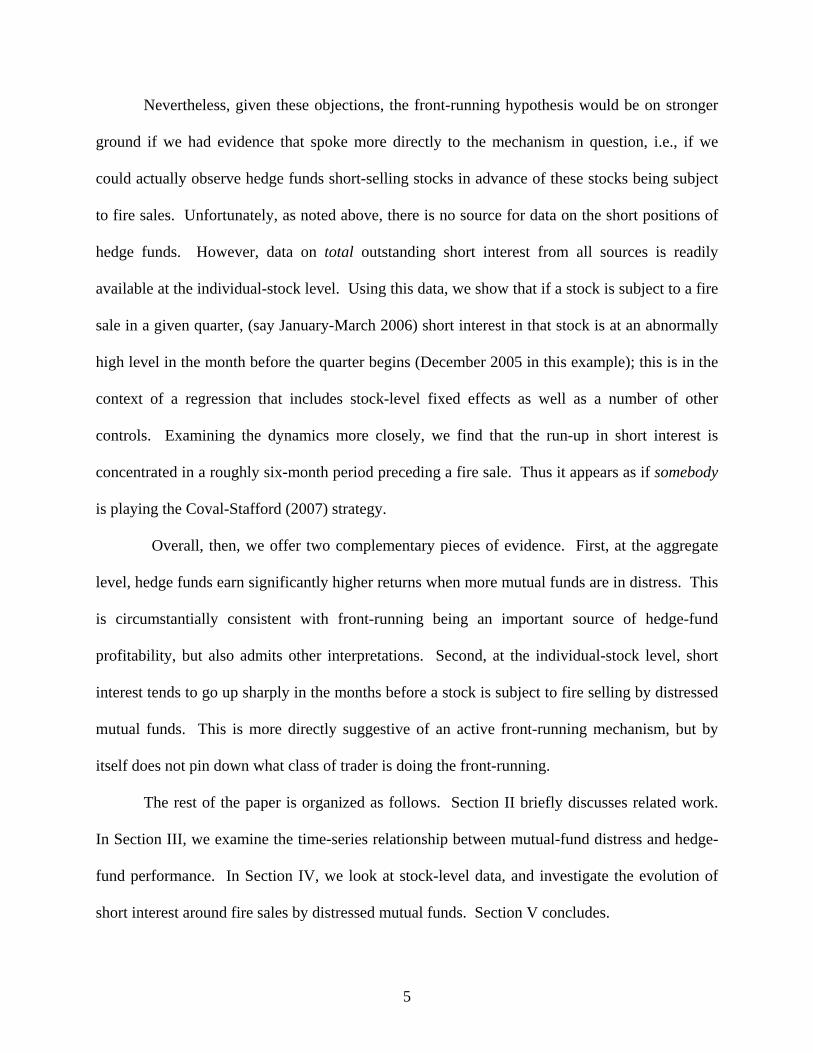
Nevertheless, given these objections, the front-running hypothesis would be on stronger

ground if we had evidence that spoke more directly to the mechanism in question, i.e., if we

could actually observe hedge funds short-selling stocks in advance of these stocks being subject

to fire sales. Unfortunately, as noted above, there is no source for data on the short positions of

hedge funds. However, data on total outstanding short interest from all sources is readily

available at the individual-stock level. Using this data, we show that if a stock is subject to a fire

sale in a given quarter, (say January-March 2006) short interest in that stock is at an abnormally

high level in the month before the quarter begins (December 2005 in this example); this is in the

context of a regression that includes stock-level fixed effects as well as a number of other

controls. Examining the dynamics more closely, we find that the run-up in short interest is

concentrated in a roughly six-month period preceding a fire sale. Thus it appears as if somebody

is playing the Coval-Stafford (2007) strategy.

Overall, then, we offer two complementary pieces of evidence. First, at the aggregate

level, hedge funds earn significantly higher returns when more mutual funds are in distress. This

is circumstantially consistent with front-running being an important source of hedge-fund

profitability, but also admits other interpretations. Second, at the individual-stock level, short

interest tends to go up sharply in the months before a stock is subject to fire selling by distressed

mutual funds. This is more directly suggestive of an active front-running mechanism, but by

itself does not pin down what class of trader is doing the front-running.

The rest of the paper is organized as follows. Section II briefly discusses related work.

In Section III, we examine the time-series relationship between mutual-fund distress and hedge-

fund performance. In Section IV, we look at stock-level data, and investigate the evolution of

short interest around fire sales by distressed mutual funds. Section V concludes.

6

II. Related Literature

While there is much anecdotal discussion of front-running, there are few systematic

empirical studies of this phenomenon. The one exception we know of is an interesting piece by

Cai (2003), who uses a unique dataset of audit trail transactions to examine the trading behavior

of market makers in the Treasury bond futures market when LTCM faced binding margin

constraints in 1998. Cai finds that market makers engaged in front-running against customer

orders coming from a particular clearing firm—orders that closely matched various features of

LTCM’s trades through Bear Stearns. The market makers traded on their own accounts in the

same direction as the customers of this clearing firm did, but one or two minutes beforehand.

There is a large literature on the determinants of hedge-fund returns. An important strand

of this work emphasizes loading on tail risks as a source of hedge-fund returns. In an early

study, Fung and Hsieh (1997) show that the distributional properties of hedge-fund returns can

differ significantly from those of mutual funds. For instance, trend-following strategies (Fung

and Hsieh (2001)) and risk-arbitrage strategies (Mitchell and Pulvino (2001)) have the sort of

highly nonlinear risk-return characteristics associated with the writing of options.

Agarwal and Naik (2004) extend this analysis to a wide variety of hedge fund styles.

They find that tail risk, as proxied by the returns to S&P 500 index options, is important for

explaining the returns of several hedge fund styles.3 From our perspective, however, it turns out

that tail risk is less of an issue. Agarwal and Naik show that the returns on long-short equity

funds—the type of fund that we focus on here—can largely be explained by the Fama-French

3 Most of the aforementioned studies look at the returns of various hedge-fund indices. But there is also evidence using individual fund return data, which shows that those funds that take on high left-tail risk outperform those funds with less risk exposure (Bali, Gokcan, and Liang (2007)).

7

(1993) three-factor model, a finding which we confirm below.4 Moreover, the nonlinear risks

associated with writing options play a statistically insignificant role for this particular strategy.

Another important consideration when looking at hedge-fund returns is the ability of

funds to smooth their reported performance (Asness, Krail and Liew (2001) and Getmansky, Lo

and Makarov (2004)). This implies that it can be important to account for past market

movements in explaining current fund returns, particularly for styles that trade relatively illiquid

securities, or that are otherwise non-transparent. Most recently, a number of studies point out

that contagion risk might also be important for explaining hedge-fund returns (Boyson, Stahel,

and Stulz (2006), Chan, Getmansky, Haas, and Lo (2006), Adrian and Brunnermeier (2007)).

In the spirit of this prior work, one contribution of our paper is to put forth a new factor—

namely aggregate mutual-fund distress—that helps to explain the time series of hedge-fund

returns. Whether or not one believes the front-running interpretation that we attach to our time-

series results, the mutual-fund distress factor appears to be a robust and economically important

determinant of the returns to long-short equity hedge funds. Moreover, at a minimum, it is a

factor that can be said to be well-motivated by a particular economic theory.

III. Mutual-Fund Distress and Hedge-Fund Returns: Time-Series Evidence

A. Data Sources

1. Hedge-fund returns

Our data on hedge-fund returns come from two providers: Credit Suisse/Tremont

(formerly Tremont Advisory Shareholder Services, or TASS); and Hedge Fund Research Inc.,

henceforth HFR. Each provider computes numerous sub-indices, corresponding to a variety of

4 Gatev, Goetzmann, and Rouwenhorst (2006) find that the Fama-French (1993) factors are also important for explaining the profitability of pairs-trading strategies.

8

different hedge-fund strategies. Given that our interest is in funds that trade in equities, and that

can take short positions, we focus primarily on the Long/Short Equity index from CS/Tremont,

and on the Equity Hedge index from HFR.5 However, in the spirit of a placebo check, we also

experiment with fixed income and global macro indices from each provider.6 The premise is that

funds in these latter categories are less likely to be active in the stock market, so their returns

should not be as sensitive to distress on the part of equity mutual funds.

The principal difference between the CS/Tremont and HFR indices is that the former are

value-weighted, while the latter are equal-weighted. More specifically, the CS/Tremont indices

are based on the net-asset-value-weighted returns of the largest funds in their universe, funds that

in each case collectively comprise at least 85 percent of the net assets under management in the

given category. The HFR indices, by contrast, equal-weight the funds in their universe. In order

to be eligible for the HFR universe, a fund must have at least $50 million under management or

have been actively trading for at least twelve months.

As is well known, hedge-fund reporting to these providers is voluntary, so no single

provider offers a comprehensive picture of the returns of all hedge funds. 7 Nevertheless, there is

reason to believe that, taken together, the CS/Tremont and the HFR data capture a substantial

fraction of the hedge-fund universe. For example, working with a larger dataset that includes

four providers (our two plus CISDM and MSCI), Agarwal et al (2007) note that as of year-end

5 According to HFR, the Equity Hedge category was the single largest hedge fund strategy as of year-end 2006, with nearly 30% of industry net assets ($409 billion out of a total of $1.427 trillion). 6 As of August 2007, the composite CS/Tremont index contained 456 funds. Of these, by far the largest number were in the Long/Short Equity index, which had 167 funds. The fixed income index was composed of 34 funds, and the global macro index contained 23 funds. 7 There are several papers that compare the indices produced by different vendors (see e.g. Agarwal and Naik (2005)), and some research that compares the indices with the returns of individual funds (Malkiel and Saha (2005)). In addition, there is some evidence that the CS/Tremont indices appear to be the least affected by various biases, perhaps because of their value-weighted nature (Malkiel and Saha (2005)).

9

2002, 63 percent of the funds in their sample were covered by either CS/Tremont or HFR.

Moreover, the overlap in the coverage of CS/Tremont and HFR is modest: only 8 percent of the

funds in the Agarwal et al sample are covered by both. This suggests that using both of these

providers gives us meaningful incremental information.8

Our sample period runs from January 1994 to December 2006. Agarwal et al (2007) and

others have argued that it is desirable to focus on the post-1994 period, since the data from 1994

onwards tends to include better coverage of defunct funds, and hence is less subject to

survivorship bias. Moreover, the CS/Tremont data are only available beginning in 1994.9

This is not to claim that survivorship bias is completely eliminated in our sample period.

However, such bias is arguably not as problematic for us as it can be in other contexts, since we

do not seek to make statements about the absolute average returns to hedge funds—i.e., we do

not address the question of whether they have unconditionally positive alphas.10 Rather, we are

interested in how their returns covary with a particular factor, namely the extent of distress in the

mutual-fund sector. It is less obvious how a bias in the data towards surviving funds would

distort our inferences about this covariance.

Table 1 presents some basic information about the monthly excess returns on the indices

that we examine. Over the 1994-2006 sample period, the equal-weighted HFR Equity Hedge

index has a somewhat higher mean monthly excess return than the value-weighted CS/Tremont

8 We have also examined data from a third provider, Barclay. Like with HFR, the Barclay indices are equal-weighted. However, they are only available beginning in 1997. Over this shorter sample period, the Barclay Equity Long/Short index produces results very similar to those we obtain below using the HFR Equity Hedge index, so we do not report them separately. 9 The HFR data go back to 1990, but again, data-quality concerns are more pronounced pre-1994. 10 The impact of survivorship bias on measured performance is analyzed by Brown, Goetzmann, and Ibbotson (1999). The related problems of termination and self-selection biases are studied by Ackermann, McEnally, and Ravenscraft (1999).

10

Long/Short Equity index, 0.83% vs. 0.68%.11 It also has a lower standard deviation, 2.51% vs.

2.89%. But perhaps most relevant for our purposes, these two indices have a very high

correlation coefficient of 0.91. This gives us some confidence that, whatever their

idiosyncrasies, they capture an essential common component of performance among long/short

equity hedge funds.

2. Measures of mutual-fund distress

To measure mutual-fund distress, we begin with a sample of funds classified as “equity”

funds using the objective codes in the CRSP Mutual-Fund Database. This screen leads us to

exclude bond funds, money market funds, sector funds, international funds and balanced funds.

To make it into our sample, a fund must also be identified in the MFLINKS database of WRDS.

In cases where there are multiple fund share classes, we aggregate these classes into one fund, on

a value-weighted basis.

Next, for each mutual fund j in each period t, we calculate FLOWj,t, which is the

percentage flow into the fund over the period. It is defined as:

FLOWj,t = (TNAj,t – (1 + rj,t)TNAj,t-1)/TNAj,t-1, (1)

where TNAj,t-1 is the total net assets under management at the end of the previous period, and rj,t

is the return (net of fees and expenses) over the period. We compute FLOWj,t at both the

monthly and quarterly frequencies.

11 This difference in mean excess returns could potentially reflect a greater degree of survivorship bias among smaller hedge funds, which play a bigger role in the equal-weighted HFR indices.

11

At either frequency, a fund is considered to be in distress if it experiences percentage

outflows greater than some threshold level. Table 2 gives a sense of how many funds are

classified as distressed, depending on the threshold that we use. For example, with a monthly

threshold of 4%, we label 7.9% of funds as distressed in a typical month, and these funds on

average represent 2.4% of assets under management among the funds in our sample. (This

difference reflects the fact that small funds have more volatile flows and hence are more likely to

become distressed than large funds.) In what follows, we use a monthly threshold of 4% as our

baseline definition of distress, but our results are robust to a wide range of alternative cutoffs.12

Once we have defined a set of distressed funds in each period, we create two measures of

aggregate distress. The first, “equal-weight outflows from distressed funds” is an equal-

weighted average of: i) the absolute value of percentage outflows (i.e., the absolute value of

FLOWj,t) from those mutual funds in distress in period t; and ii) zero for those mutual funds not

in distress in period t. The second, “asset-weight outflows from distressed funds” is an assets-

under-management-weighted average of: i) the absolute value of percentage outflows from those

mutual funds in distress in period t; and ii) zero for mutual funds not in distress in period t. 13

Note that our sign convention is that more positive values of these measures are associated with

greater mutual-fund distress.14

12 Yan (2006) documents that over the period 1992-2001, the median equity mutual fund held a cash balance equal to 3.68% of assets. Thus for a typical fund, an outflow of 4% in a month would necessarily lead to some forced liquidations of its stockholdings. 13 For the purposes of these calculations (and after we have already classified funds as distressed or not) we winsorize FLOWj,t at its 5% and 95% values within each period. We do so because there are a number of extreme outliers in the flow numbers, including some cases where measured outflows from a fund exceed 100%. Per equation (1), this is presumably due in part to a mismeasurement of the fund’s return rj,t. However, our results are qualitatively similar—albeit a bit noisier—if we do not winsorize at all. 14An alternative approach to measuring aggregate distress is simply to count—on either an equal-weighted or value-weighted basis—the fraction of funds that are distressed at any point in time. We view this approach as somewhat less desirable, as it amounts to focusing only on the extensive distress margin, and ignoring the intensive margin—

12

Of the two measures, the latter, asset-weighted one is perhaps more immediately

intuitive: it simply captures total dollar outflows from all distressed funds, scaled by the current

size of the mutual-fund sector. Nevertheless, we believe that the equal-weight measure also has

some conceptual appeal, particularly to the extent that small distressed funds offer proportionally

more opportunities for front-running than large distressed funds. For example, since small funds

tend to hold fewer stocks than large funds, they have less choice of what to unload when they get

into trouble, and hence their trades may be easier for a front-runner to predict. By putting

relatively more weight on the outflows of such small funds, the equal-weight distress measure

arguably does a better job of incorporating this effect.

Figure 1 plots these two aggregate distress measures on a monthly basis over the period

1994-2006, using a 4% threshold to define distress. While the equal-weight measure is

considerably more volatile, the two are closely correlated, with a correlation coefficient of 0.859.

Thus it should come as no surprise that our results below are not sensitive to which of the two

measures we use. Another point to note is that there is a distinct tendency for the distress

measures to spike up in the month of December.

B. Results

1. Baseline specification

Panels A and B of Table 3 present the results from our baseline time-series specification,

using the value-weighted CS/Tremont Long/Short Equity index, and the equal-weighted HFR

Equity Hedge index, respectively. Consider first Panel A, which focuses on the CS/Tremont

index. In column (1), we warm up with a conventional performance-attribution regression, in

i.e., it ignores the size of the outflows from distressed funds. Nevertheless, it leads to results that are similar to those we report below.

13

which the monthly excess returns on the index from January 1994 through December 2006 are

regressed against four familiar factors: MKTRF, the excess return on the value-weighted market

portfolio; SMB, the return on a portfolio that is long small stocks and short large stocks; HML,

the return on a portfolio that is long high book-to-market stocks and short low book-to-market

stocks; and UMD, the return on a portfolio that is long past twelve-month winners and short past

twelve-month losers. Of these factors, MKTRF, SMB and UMD come in strongly positive and

significant, and collectively they explain an impressive amount of the variation of the returns to

the Long/Short Equity index: the simple R-squared of the regression is 80.1%. This is consistent

with prior work (Agarwal and Naik (2004)) which finds that for long-short equity funds, linear

stock-market factors are the most important explanatory variables, with non-linear option-like

factors playing a statistically insignificant role.

In column (2), we add to these four factors the contemporaneously-measured monthly

variable DISTRESS, which is just “equal-weight outflows from distressed funds”, as described

above, using a monthly threshold level of 4%. The coefficient on DISTRESS is 1.703, and is

statistically significant, with a t-stat of 3.17. To get a sense of the economic magnitude of this

effect, note that the standard deviation of the DISTRESS variable is 0.230%, which implies that

a one-standard-deviation increase in DISTRESS raises monthly hedge-fund returns by 39.2 basis

points, or almost five percentage points on an annualized basis.

In column (3), we keep all else the same as column (2), but add also POSFLOW, which is

the mirror image of DISTRESS—i.e., it captures equal-weighted inflows to those mutual funds

that have positive inflows of greater than 4%. The motivation for including this variable also

comes from Coval and Stafford (2007), who note that mutual funds experiencing large inflows

often tend to mechanically scale up their existing positions, rather than diversifying into new

14

holdings. Thus, Coval and Stafford suggest, large inflows may also give rise to predictable price

pressure—a phenomenon they refer to as “fire purchases”—and hence to front-running

opportunities. As it turns out, however, the coefficient on POSFLOW, while of the expected

positive sign, is much smaller than that on DISTRESS, and is statistically insignificant.

In column (4), we add lagged values of MKTRF, SMB, HML, UMD, and DISTRESS to

the specification from column (2). The lagged values of the MKTRF, SMB, HML, and UMD are

motivated by prior work which shows that measured hedge-fund returns can be sluggish in

adjusting to market-wide price movements, perhaps due to smoothing of reported performance

by fund managers (Asness, Krail, and Liew (2001) and Getmansky, Lo, and Makarov (2004)).

And indeed, the returns to the CS/Tremont index show a significant loading on the lagged value

of MKTRF. However, these extra controls have little effect on the contemporaneous DISTRESS

term, which, at a value of 1.589, remains strongly significant. And interestingly, the coefficient

on lagged DISTRESS in this regression is close to zero, and is not statistically significant.

The fact that lagged DISTRESS is insignificant cuts against a liquidity-provision

interpretation of our results, since as Coval and Stafford (2007) show, the mean reversion that

occurs after a fire sale plays out gradually, over the course of roughly 18 months. Thus one

would expect a liquidity provider to earn higher returns for several months after a period of

increased distress. In contrast, the contemporaneous nature of the link between DISTRESS and

hedge-fund returns is more consistent with front-running, since a front-runner presumably closes

out his position and takes his profit at the moment that a fire sale occurs.

In column (5), we further explore the timing of the relationship between DISTRESS and

hedge-fund returns, by adding a single lead of DISTRESS to the specification from column (4).

Here we find that the contemporaneous and lead terms of DISTRESS share the explanatory

15

power for returns, with the lead term actually being somewhat larger (1.595 vs. 1.077) and more

statistically significant. One possible explanation for this result is that mutual funds are able to

partially anticipate large outflows, and begin preparing themselves by selling stocks (and hence

increasing their cash balances) in the month before an outflow hits. Thus some of the fire-sale

activity associated with a large month-t outflow may start to show up in month t-1. This story

has the testable implication that an increase in total mutual-fund cash balances in month t-1

should portend a rise in the DISTRESS variable in month t.

Panel B replicates everything in Panel A, but using the equal-weighted HFR Equity

Hedge index instead of the value-weighted CS/Tremont index. The conclusions that emerge are

generally quite similar, though a few noteworthy distinctions stand out. First, using an equal-

weighted index reduces the noise in measured hedge-fund returns, leading to uniformly higher R-

squareds and t-statistics. For example, in column (2), the coefficient on DISTRESS is now 2.014

with a t-stat of 4.21, and the R-squared is 86.8%, as opposed to its value of 81.8% in the

corresponding column (2) of Panel A.

Second, with these more precise estimates, the coefficient on POSFLOW in column (3)

now becomes statistically significant, although it remains much smaller, at 0.462, than the

coefficient on DISTRESS. Thus the HFR data offer some support for the proposition that there

may also be front-running opportunities associated with large inflows into mutual funds.

Nevertheless, it would seem that the magnitude of this effect is not nearly as large as that

associated with outflows from distressed funds—a conclusion which seems quite plausible.

Third, the lead-lag relationship between hedge-fund excess returns and DISTRESS looks

a bit different using the HFR data. Specifically, the coefficient on the first lead of DISTRESS in

16

column (5) of Panel B is close to zero and no longer significant; to a first approximation, what

matters in this regression is just the contemporaneous DISTRESS term.

2. A graphical illustration

Figures 2 and 3 illustrate the regression results discussed above. In Panel A of Figure 2,

we create a series of monthly alphas, defined as the residuals from a regression of the returns on

the CS/Tremont index on the four factors MKTRF, SMB, HML, UMD, and a constant. We then

plot these alphas against the residuals from a regression of DISTRESS on the same four factors.

Thus, the slope of the line in this scatterplot corresponds to the OLS coefficient on DISTRESS

from column (2) in Panel A of Table 3. In Panel B, we plot the joint time-series evolution of

these same two residuals. In Figure 3, we repeat all of this, using instead the HFR index.

As can be seen from the scatterplots, the regression results that we report appear to

capture a central tendency of the data, as opposed to just a handful of extreme outliers. At the

same time, it is apparent from the time-series plots that the years 1998 to 2000 contribute in an

important way to our results, since this is a period of especially high volatility in the DISTRESS

variable. We do not view this as a shortcoming. Rather, one might say that the extreme fund

flows during the dotcom era are a blessing for our methodology, since they provide much of the

variation in our key right-hand-side variable, thereby increasing the power of our tests.

3. Additional controls

In Panel C of Table 3, we add a variety of additional controls to the baseline regressions

from column (2) in Panels A and B. Specifically, we add: i) MKTVOL, the standard deviation

of daily market returns in the given month (in column 1); ii) XVOL, the cross-sectional standard

17

deviation of monthly individual-stock returns in the given month (in column 2); iii) TIME and

TIME squared, where TIME is the numbers of years since the start of the sample period (in

column 3); and iv) DEC, a dummy variable that takes on the value of one in the month of

December (in column 4).

The MKTVOL and XVOL variables represent an attempt to control for the possibility

that mutual-fund distress is more likely to occur when markets are going through periods of high

volatility. The TIME and TIME squared terms are meant to take out any low-frequency time

trends in the data. And finally, the DEC dummy is added in light of Agarwal et al (2007), who

uncover a December seasonal in hedge fund returns—an effect that they attribute to managers’

efforts to inflate year-end performance. Their finding is particularly relevant for us, since

mutual-fund outflows, and hence our DISTRESS variable, also tend to be elevated in December.

As it turns out, none of these added controls materially affect our key results. For

example, focusing on the CS/Tremont Long/Short Equity index, the coefficient on DISTRESS

ranges from 1.544 to 1.960 across the four columns (and remains significant in each case); these

figures compare with the value of 1.703 in the less heavily-controlled version of the same

regression in column (2) of Panel A. Turning to the HFR Equity Hedge index, the coefficient on

DISTRESS ranges from 1.649 to 2.246 across the four columns; these figures compare with the

value of 2.014 in column (2) of Panel B. 15

4. Results for fixed income and global macro hedge funds

In Panel D of Table 3, we re-run our baseline specification using fixed income and global

macro indices from both CS/Tremont and HFR. These regressions can be thought of as a

15 If we add all of these additional controls jointly, the results remain significant: for the CS/Tremont index, the coefficient on DISTRESS is 1.242 (t-statistic of 2.01), while for the HFR index it is 2.079 (t-statistic of 5.07).

18

placebo check on our results. In particular, given that fixed income and global macro funds are

less likely to be active traders of equities, we should expect their returns to be less strongly

influenced by distress among equity mutual funds.16 And, as can be seen, there is no evidence of

a systematic positive relationship between the DISTRESS variable and hedge-fund returns in

either fixed income or global macro. Across all the specifications in Panel D, the coefficient on

DISTRESS is never statistically significant.

5. Varying measures of mutual-fund distress

All of the results thus far are based on just a single version of our mutual-fund distress

measure. We have always been equal-weighting the outflows of distressed funds, and have been

consistently using a monthly distress threshold of 4%. In Table 4, we explore a wide range of

variations with respect to these choices. In each case, we run a regression of monthly hedge-

fund excess returns on a particular measure of mutual-fund distress, and on the four factors

MKTRF, SMB, HML, and UMD. Thus, the regressions are directly comparable to those in

column (2) of Table 3, Panels A and B. However, to save space, each column of Table 4 shows

only the coefficient on the given distress measure; the coefficients on the other four factors are

suppressed. Using this format, we examine both equal-weighted and asset-weighted distress

measures with thresholds ranging in one-percent increments from 2% to 6%. Altogether, these

combinations yield 10 different proxies. Panel A of Table 4 uses the CS/Tremont Long/Short

Equity index to create our dependent variable, and Panel B uses the HFR Equity Hedge index.

16 We cannot rule out that funds in these categories do some equity trading. Indeed, the returns to both HFR indices load significantly on the stock-market factors MKTRF, SMB, and HML, and the HFR global macro index also loads on UMD. These four factors explain 33.4% of the variation in the HFR fixed income index, and 33.0% of the variation in the HFR global macro index. The HFR fixed income index (unlike the CS/Tremont fixed income index) includes convertible bond funds, which could help to explain its exposure to stock-market factors.

19

When looking at the results in Table 4, it should be borne in mind that the coefficients on

two different distress measures are not directly numerically comparable to one another, as they

can have very different standard deviations. Thus to ease comparability, we report below each

coefficient the implied effect of a one-standard deviation change in the given distress measure.

With this metric, it can be seen that the results are generally of a consistent magnitude across the

whole range of distress measures.

In Panel A, with the CS/Tremont index, a one-standard-deviation increase in any of the

equal-weighted distress measures raises monthly hedge-fund returns by just under 40 basis

points, while a one-standard-deviation increase in any of the asset-weighted measures increases

returns by roughly 30 bps. In Panel B, with the HFR index, there is a bit more variability across

the distress measures, with the economic impact of a one-standard-deviation shock ranging from

39 to 47 bps for the equal-weighted measures, and from 32 to 39 bps for the value-weighted

measures. Nevertheless, the overall picture that emerges is one of uniformity across the various

distress measures. Of course, this should not be too surprising, as these measures are all highly

correlated with one another in the time series.

6. Dollar magnitudes

The above estimates can also be mapped into a statement about how many dollars long-

short equity hedge funds gain from each incremental dollar that flows out of a distressed mutual

fund. Note that in the specifications in the right-hand block of Table 4 Panel A, the asset-

weighted distress measures are based on the dollar value of outflows from distressed funds,

scaled by total mutual-fund assets. Similarly, the CS/Tremont index reflects asset-weighted

hedge-fund returns. Therefore, we can recover dollar hedge-fund returns per dollar of distress

20

flows simply by multiplying the estimated coefficient on DISTRESS by the ratio of hedge-fund

assets to mutual-fund assets.

Unfortunately, because of the explosive growth of hedge funds, this relative-size ratio is

highly variable over our sample period. This makes our inferences sensitive to the year upon

which the calibration is based. Consider as a first example year-end 1997, which is about one-

third of the way through our 13-year sample period. The value of equities held by open-end

mutual funds was $2.019 trillion as of this date, while, according to HFR, total assets under

management in the Equity Hedge category were $20.4 billion.17 These figures imply a relative-

size ratio of 1.01%. If we multiply this ratio by the coefficient of 2.725 on DISTRESS in the

right-hand block of panel A (this is the coefficient corresponding to a distress threshold of 4%)

we obtain a value of 2.75%. In other words, for each additional dollar of distressed mutual-fund

outflows, the returns of long-short equity hedge funds go up by 2.75 cents. If we define distress

using a threshold of 2% instead of 4%, the coefficient estimate of 1.613 in Panel A of Table 4,

multiplied by the same ratio of 1.01%, yields a figure of 1.63 cents per dollar of outflows.

These magnitudes are quite modest. However, if we instead base our calculations on

year-end 2001—roughly two-thirds of the way through our sample period—things look very

different. The relative-size ratio has by this point risen to 6.10%, implying that long-short equity

hedge funds gain 16.62 cents for each incremental dollar of mutual-fund distress if we define

distress using a 4% threshold, or 9.84 cents if we define distress using a 2% threshold. These

latter numbers would seem to be at the upper end of any plausible range. We suspect that the

truth lies somewhere in between, but it is hard to say where.

17 The figure for mutual funds comes from table L.122 of the Federal Reserve’s Flow of Funds Accounts. HFR’s Equity Hedge category closely mirrors CS/Tremont’s Long/Short category, so their estimate of total assets under management in this segment roughly captures the size of the universe of long-short funds that we have been focusing on in our regressions.

21

IV. Does Short Interest Rise in Advance of Fire Sales by Distressed Mutual Funds?

A. Data and Variable Construction

Our data on monthly short interest for NYSE, AMEX and NASDAQ stocks are obtained

from Bloomberg. We use this data to construct short interest ratios for each stock in each month.

Observations on short interest represent positions that close on the first business day on or after

the 15th of the month. Hence we approximate the short interest ratio by dividing total short

interest by shares outstanding on the closest available day to the 15th of each month. Because the

resulting raw short interest ratio, denoted by SR, is strongly right-skewed, in our regressions we

use as a dependent variable a log transform LSR, which is given by LSR = log(SR + 0.01%), and

which is more symmetrically distributed than SR.

Our key right-hand side variable is a measure of fire-selling by distressed mutual funds in

a particular stock. We construct this measure as follows. First, for each quarter ending in

March, June, September or December, and for each stock in our universe, we calculate the

number of shares bought or sold by every mutual fund in the CDA/Spectrum database that

reports holdings at both the beginning and end of the quarter. (These changes in shareholdings

control for stock splits.) Next, we define a mutual fund as distressed at the 8% level if it has had

outflows of greater than 8% over the quarter. From Panel B of Table 2, this definition

encompasses 11.7% of funds and 3.9% of fund assets in a typical quarter. The variable

FIRESALE{8} is then defined for each stock as the sum of all shares sold by distressed funds in

a quarter, divided by shares outstanding. In symbols, for stock i in quarter t we compute:

{ }{ } { }, , ,

,,

max 0, j i t j tji t

i t

Holdings I Flow ThreshFIRESALE Thresh

SharesOutstanding

−Δ × < −=∑

, (2)

22

where ΔHoldingsj,i,t is the change in fund j’s holdings of stock i during the quarter.18

Finally, we denote by FIRESALE{8,90} an indicator that takes on the value one

whenever the continuous variable FIRESALE{8} exceeds the 90th percentile value for all stocks

in the same NYSE size tercile, and that takes on the value zero otherwise.19 FIRESALE{8,90} is

our baseline measure of whether a stock is subject to a fire sale in a given quarter. Note that we

use the entire panel unconditionally to determine the 90th percentile cutoffs, which means that,

according to our definition, there may be more fire sales in some periods than others. In other

specifications, we also use variables we denote as FIRESALE{8,95}, FIRESALE{6,90} and

FIRESALE{10,90}. These variables are constructed analogously, but using either different

percentile breakpoints in the FIRESALE{8} distribution, or different thresholds for determining

mutual-fund distress.

When we examine the impact of sales by distressed mutual funds, we want to be careful

to distinguish this from any impact of sales by other, non-distressed mutual funds. Thus a crucial

control is SELL, which is simply the total gross number of shares sold in a quarter by all mutual

funds, divided by shares outstanding at the end of the quarter. Similarly, BUY is the total gross

number of shares bought in a quarter by all mutual funds, divided by shares outstanding.

In addition to these variables, our regressions include a number of other controls that

have been found in previous work (e.g., D’Avolio (2002), Asquith et al (2005), and Savor and

Gamboa-Cavazos (2005)) to be significant determinants of short interest. These include

18 Our FIRESALE variable is comparable to the PRESSURE_3 variable constructed by Coval and Stafford (2007). 19 Cutoffs are computed by NYSE size terciles in order to allow us to easily study size interactions below. The cutoffs are always highest for the middle tercile and lowest for the smallest tercile of stocks. Consistent with our findings on the size interactions, if the cutoff is not conditioned on size tercile, the magnitude of the resulting coefficients are in line with those obtained for the middle tercile of firms, and continue to be highly significant.

23

institutional ownership, firm size, turnover, book-to-market, past returns, and the presence of

convertible bonds in the firm’s capital structure.

Our institutional ownership measure, IHOLD, is based on the CDA Spectrum Database

of 13-F filings by large institutional investors, defined as those managing at least $100 million

dollars in assets. Specifically, IHOLD is the fraction of a company’s shares that are held by 13-F

institutions, measured at the end of each calendar quarter.

The remaining controls are based on data from the Center for Research in Security Prices

(CRSP) and COMPUSTAT.20 With respect to firm size, rather than simply including a linear

size control, we are more expansive, and use a set of 20 dummy variables corresponding to demi-

deciles of the NYSE market-cap distribution in each period. We do so because the relationship

between short interest and firm size is highly non-linear. In particular, short interest has an

inverted-U shape when plotted against size: it is low among the very smallest micro cap stocks,

then rises sharply with size through the first two deciles of the size distribution, before flattening

out and eventually declining with size through the last two deciles of the size distribution

Our turnover measure, TURN, is a firm’s turnover in a quarter. BM is a firm’s book

value divided by market capitalization at the end of the most recent fiscal year. PRET is a firm’s

stock return over the past twelve months. CONVERT is a dummy that equals one if a firm has

convertible debt outstanding at the end of its most recent fiscal year, and zero otherwise. Table 5

displays the full-panel means and standard deviations of all of the variables described above. In

Table 5, and in the analysis that follows, all variables except IHOLD and CONVERT are

winsorized at their 1% and 99% values within each quarter.

20 To be included in our sample, a firm must have the requisite financial data from both CRSP and COMPUSTAT, which include book value, market capitalization, and twelve months of past returns. We also follow other studies in focusing on stocks with CRSP share codes of 10 or 11, i.e., common stocks of U.S. firms that are listed on the NYSE, AMEX or NASDAQ.

24

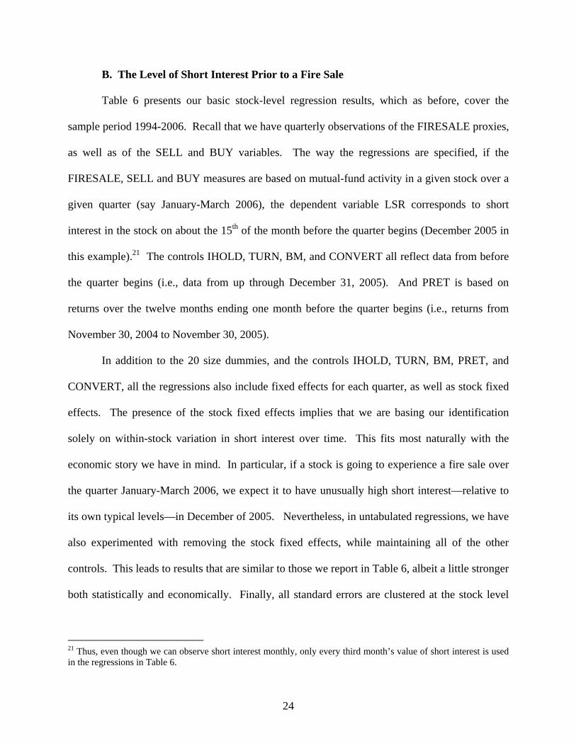
B. The Level of Short Interest Prior to a Fire Sale

Table 6 presents our basic stock-level regression results, which as before, cover the

sample period 1994-2006. Recall that we have quarterly observations of the FIRESALE proxies,

as well as of the SELL and BUY variables. The way the regressions are specified, if the

FIRESALE, SELL and BUY measures are based on mutual-fund activity in a given stock over a

given quarter (say January-March 2006), the dependent variable LSR corresponds to short

interest in the stock on about the 15th of the month before the quarter begins (December 2005 in

this example).21 The controls IHOLD, TURN, BM, and CONVERT all reflect data from before

the quarter begins (i.e., data from up through December 31, 2005). And PRET is based on

returns over the twelve months ending one month before the quarter begins (i.e., returns from

November 30, 2004 to November 30, 2005).

In addition to the 20 size dummies, and the controls IHOLD, TURN, BM, PRET, and

CONVERT, all the regressions also include fixed effects for each quarter, as well as stock fixed

effects. The presence of the stock fixed effects implies that we are basing our identification

solely on within-stock variation in short interest over time. This fits most naturally with the

economic story we have in mind. In particular, if a stock is going to experience a fire sale over

the quarter January-March 2006, we expect it to have unusually high short interest—relative to

its own typical levels—in December of 2005. Nevertheless, in untabulated regressions, we have

also experimented with removing the stock fixed effects, while maintaining all of the other

controls. This leads to results that are similar to those we report in Table 6, albeit a little stronger

both statistically and economically. Finally, all standard errors are clustered at the stock level

21 Thus, even though we can observe short interest monthly, only every third month’s value of short interest is used in the regressions in Table 6.

25

since we are concerned about temporary stock-level effects which may not be fully absorbed by

the stock fixed effects.22

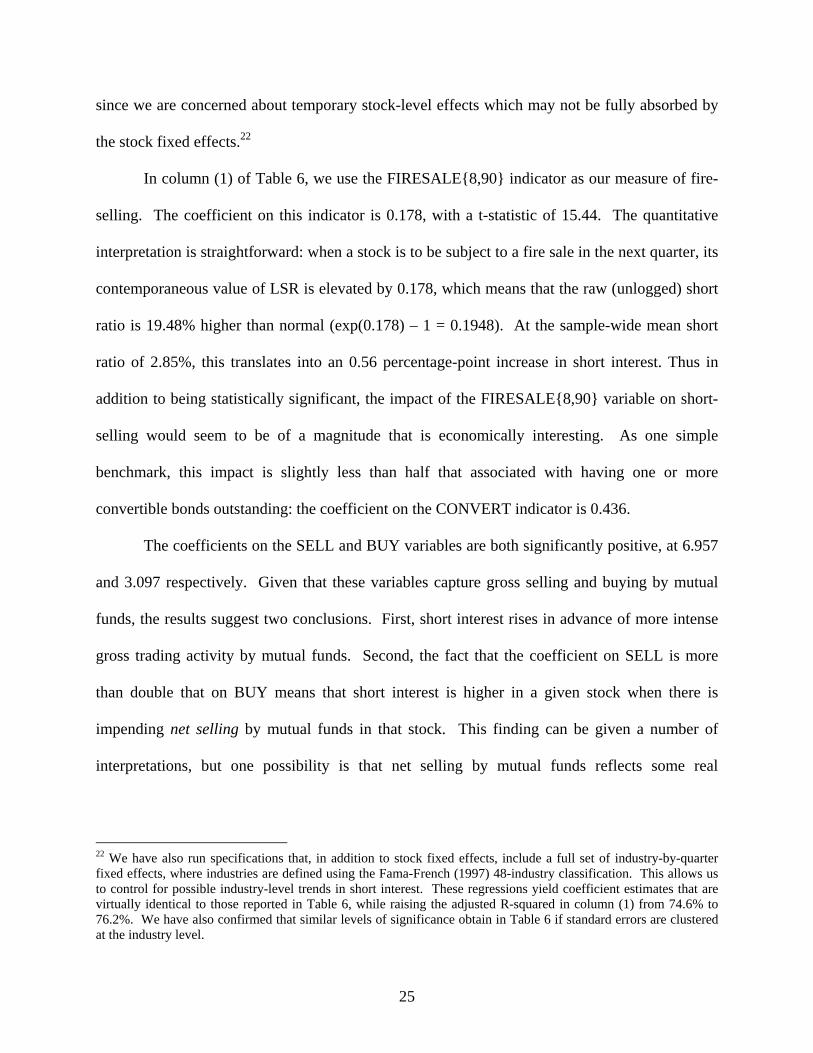
In column (1) of Table 6, we use the FIRESALE{8,90} indicator as our measure of fire-

selling. The coefficient on this indicator is 0.178, with a t-statistic of 15.44. The quantitative

interpretation is straightforward: when a stock is to be subject to a fire sale in the next quarter, its

contemporaneous value of LSR is elevated by 0.178, which means that the raw (unlogged) short

ratio is 19.48% higher than normal (exp(0.178) – 1 = 0.1948). At the sample-wide mean short

ratio of 2.85%, this translates into an 0.56 percentage-point increase in short interest. Thus in

addition to being statistically significant, the impact of the FIRESALE{8,90} variable on short-

selling would seem to be of a magnitude that is economically interesting. As one simple

benchmark, this impact is slightly less than half that associated with having one or more

convertible bonds outstanding: the coefficient on the CONVERT indicator is 0.436.

The coefficients on the SELL and BUY variables are both significantly positive, at 6.957

and 3.097 respectively. Given that these variables capture gross selling and buying by mutual

funds, the results suggest two conclusions. First, short interest rises in advance of more intense

gross trading activity by mutual funds. Second, the fact that the coefficient on SELL is more

than double that on BUY means that short interest is higher in a given stock when there is

impending net selling by mutual funds in that stock. This finding can be given a number of

interpretations, but one possibility is that net selling by mutual funds reflects some real

22 We have also run specifications that, in addition to stock fixed effects, include a full set of industry-by-quarter fixed effects, where industries are defined using the Fama-French (1997) 48-industry classification. This allows us to control for possible industry-level trends in short interest. These regressions yield coefficient estimates that are virtually identical to those reported in Table 6, while raising the adjusted R-squared in column (1) from 74.6% to 76.2%. We have also confirmed that similar levels of significance obtain in Table 6 if standard errors are clustered at the industry level.

26

information about fundamentals, and that whoever is taking short positions is acting on that same

information in a somewhat more timely fashion.

In light of this story, it is important to stress that the coefficient on FIRESALE{8,90}

reflects an incremental impact of selling by distressed mutual funds, above and beyond the

impact of selling by all mutual funds (which is embodied in SELL). Thus our results for the

FIRESALE{8,90} variable cannot be explained away simply by saying that short-sellers are

responding to the same information as mutual funds in general; this effect will be absorbed by

the SELL and BUY controls. Rather, there seems to be something special about sales by

distressed mutual funds.

The other controls in the regression have the signs that one would expect based on

previous work. Short interest is increasing in turnover and institutional ownership, and as

already noted, is higher when the firm in question has convertible debt outstanding. Short sellers

also appear to be tilting in the right direction with respect to book-to-market and momentum, as

the coefficients on BM and PRET are significantly negative. Collectively, all the variables—

including the fixed effects—explain a large fraction of the variation in LSR: the adjusted R-

squared of the regression is 0.746.

Directly underneath the principal regression in column (1) of Table 6, we report the

results from a variant in which all the controls are the same, but in which the FIRESALE{8,90}

variable is interacted with SMALL, MID, and LARGE, which are dummies that equal one if a

stock belongs in NYSE deciles 1-2 (SMALL), 3-6 (MID), and 7-10 (LARGE), respectively. The

goal here is to decompose our full-sample results by broad market-cap categories. For brevity,

we do not reproduce the coefficients on the controls, and focus only on the key interaction terms.

27

The coefficient on FIRESALE{8,90}*SMALL is 0.287, with a t-statistic of 16.16; the

coefficient on FIRESALE{8,90}*MID is 0.090, with a t-statistic of 5.43; and the coefficient on

FIRESALE{8,90}*LARGE is -0.008, with a t-statistic of 0.38. Thus the effects of future fire

sales on short interest are strongest among small-cap stocks, continue to be economically and

statistically significant among mid-cap stocks, and are non-existent among large-cap stocks.23

This is not an implausible result, particularly if one believes that small stocks are likely to be less

liquid, and hence vulnerable to more price pressure for a given amount of fire-selling. If so, it

would be more attractive for a front-runner to take a short position in a small stock in advance of

a fire sale, all else equal.

Columns (2)-(4) of Table 6 redo the analysis of column (1), with the FIRESALE{8,95},

FIRESALE{6,90}, and FIRESALE{10,90} indicators taking the place of FIRESALE{8,90}. As

can be seen, the overall results are very similar. Thus our conclusions do not appear to be

sensitive to modest changes in the thresholds used to define a fire sale.

Finally, in column (5), we use FIRESALE{8}, which is not an indicator, but rather a

continuous variable measuring total gross selling of a stock by all distressed mutual funds. (As in

the baseline specification, distressed funds are still defined as those with outflows of greater than

8% in the quarter.) While it might be argued that this continuous measure is in some ways less

appropriate for capturing the extreme nature of a fire sale, it does have one nice feature: it is

denominated in the same units as the SELL and BUY controls. Therefore it allows for a direct

and intuitive comparison of their magnitudes. As can be seen, the coefficient on FIRESALE{8}

is 20.012 (with a t-statistic of 4.67), while the coefficient on SELL is 8.156 (with a t-statistic of

23 Although the proportional effect is larger for small stocks than for medium-sized stocks, the absolute effects are similar. Mean short interest for stocks in the smallest NYSE tercile is 1.78%, so a coefficient of 0.287 implies a 0.59 percentage point increase. For medium-sized stocks, mean short interest is 4.53%, so the implied increase based on a coefficient of 0.090 is 0.43 percentage points.

28

8.17). This means that an impending sale by a distressed mutual fund has an impact on short

interest that is more than three times the impact of an impending sale of the same size by a non-

distressed mutual fund.24

C. The Dynamics of Short Interest Around Fire-Sale Events

The above results suggest that short interest is elevated prior to fire sales by distressed

mutual funds. In other words, if a fire sale is to take place in a given stock during the quarter

January-March 2006, short interest in that stock is abnormally high in December 2005.

However, in order to shed more light on the front-running hypothesis, we would like to paint a

fuller picture of the dynamic evolution of short interest around fire-sale events. To do so, we

begin with the baseline specification from column (1) in Table 6, and add a number of event-

time dummies.

Specifically, suppose that for a given stock there is a FIRESALE{8,90} event in quarter t.

We now include in the regression a set of 13 event-time dummy variables labeled t-6, t-5,…t,

...,t+5, t+6, where our convention is that dummy k takes on the value one in the last month of

quarter k. Thus if there is a FIRESALE{8,90} event in the quarter January-March 2006, the t-1

dummy takes on the value one in December 2005, the t-2 dummy takes on the value one in

September 2005, the t-3 dummy takes on the value one in June 2005, and so on. Note that, given

this convention, the regression in column (1) of Table 6 is just a special case of this one, where

only the t-1 dummy (for December 2005) is included, and all of the other event-time dummies

are left out.

24 Note that the total impact of a sale by a distressed fund is obtained by summing the coefficients on SELL and on FIRESALE{8}.

29

It is important to recognize that more than one of the event-time dummies can be turned

on for a given stock-quarter observation. This is because fire-sale events are not necessarily

isolated, and tend to cluster in time for a given firm. Thus for example, if a stock were to be

subject to consecutive fire sales in the two quarters January-March 2006, and April-June 2006,

both the t-1 and t-2 dummies would take on the value of one in December of 2005—since

December of 2005 effectively precedes one of the fire sales by a quarter, and the other by two

quarters. The benefit of this approach is that it allows us to control for the temporal clustering of

fire sales when tracing out the evolution of short interest. The cost is that in order to implement

it fully, we need to restrict our sample to those firm-quarters for which we have data available for

the entire t-6 to t+6 window surrounding the quarter. This screen reduces the size of our panel

from the 176,341 observations used in Table 6, down to 75,562 observations.25

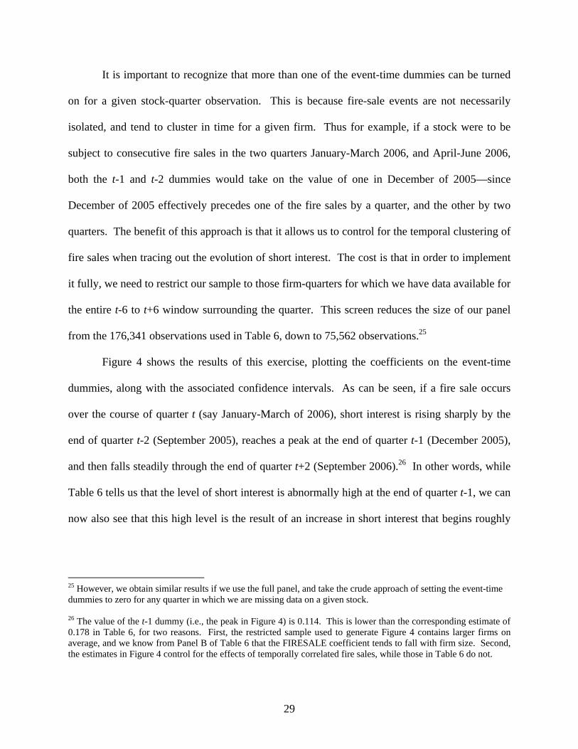
Figure 4 shows the results of this exercise, plotting the coefficients on the event-time

dummies, along with the associated confidence intervals. As can be seen, if a fire sale occurs

over the course of quarter t (say January-March of 2006), short interest is rising sharply by the

end of quarter t-2 (September 2005), reaches a peak at the end of quarter t-1 (December 2005),

and then falls steadily through the end of quarter t+2 (September 2006).26 In other words, while

Table 6 tells us that the level of short interest is abnormally high at the end of quarter t-1, we can

now also see that this high level is the result of an increase in short interest that begins roughly

25 However, we obtain similar results if we use the full panel, and take the crude approach of setting the event-time dummies to zero for any quarter in which we are missing data on a given stock. 26 The value of the t-1 dummy (i.e., the peak in Figure 4) is 0.114. This is lower than the corresponding estimate of 0.178 in Table 6, for two reasons. First, the restricted sample used to generate Figure 4 contains larger firms on average, and we know from Panel B of Table 6 that the FIRESALE coefficient tends to fall with firm size. Second, the estimates in Figure 4 control for the effects of temporally correlated fire sales, while those in Table 6 do not.

30

three to six months before the onset of a fire-sale quarter, and that starts to reverse itself once the

fire-sale quarter draws to a close.

The event-time evolution of short interest depicted in Figure 4 would appear to fit

comfortably with a front-running hypothesis. In particular, Coval and Stafford (2007) show that

fire sales can be reliably predicted several months ahead of time, based on the relationship

between mutual-fund flows and lagged mutual-fund performance. So one might expect front-

runners to begin taking short positions roughly this far in advance of a fire sale.

V. Conclusions

Rather than restate our results, we close with a couple of further qualifications regarding

how these results should be interpreted. First, even if one accepts the proposition that hedge

funds are engaging in the general kind of front-running that we describe, we cannot speak to how

they are implementing it—i.e., to what kind of data, either public or private, they are using to

construct their trading strategies. For example, it is possible that some funds are using a public-

sources methodology very similar to that laid out by Coval and Stafford (2007): studying 13-F

filings to get a picture of mutual funds’ holdings, and trying to forecast which ones will become

distressed based on past performance. On the other hand, it could be that some funds are relying

on illegal inside information from their brokers to tell them precisely when a fire sale is coming.

This more refined information set would naturally lead to higher trading profits on average.

Nevertheless, as long as there is a greater supply of such inside information when more mutual

funds are in distress, this mechanism would also generate patterns like those we observe. Thus

we have nothing to say about whether any front-running done by hedge funds is of the legal or

illegal variety.

31

Finally, and more subtly, even if front-running hedge funds earn higher returns as a result

of mutual funds being in distress, it does not necessarily follow that these incremental returns are

at the expense of mutual funds. This point is most clearly illustrated with a simple example.

Consider a stock that is trading at $100/share at time 0. At time 1, a hedge fund gets an advance

tip that a distressed mutual fund will be selling 100 shares at time 2. These shares will have to

be absorbed by the risk-averse “public”, which will cause the price to fall to $98. If the hedge

fund does not front-run, the entire price decline is delayed until time 2. Alternatively, suppose

the hedge-fund front-runs by short-selling 50 shares to the public at time 1, which drives the

price down to $99 at this time. If the hedge fund covers its position at time 2, and if the mutual

fund’s selling decision is unaffected by the time-1 price movement, the price at time 2 will still

be $98, since all of the mutual fund’s 100-share sale is again ultimately absorbed by the public.

In this example, the hedge fund clearly profits by front-running (it sells 50 shares for $99

and buys them back at $98), but the distressed mutual fund is no worse off, since it sells its 100

shares for $98 at time 2 in either case. Rather, it is the public that is harmed by front-running,

since instead of getting to buy 100 shares for $98, the public buys 50 shares for $99 at time 1 and

another 50 shares for $98 at time 2. Intuitively, by using its inside information about the

impending fire sale, the hedge fund is able to exploit public investors, who, not knowing the fire

sale is coming, are content to buy at $99 at time 1. As a result, the public earns less from

liquidity provision than it otherwise would.

None of this is meant to argue that a distressed mutual fund cannot be hurt by a front-

runner with advance knowledge of its trades; indeed, it is easy to construct alternative scenarios

where the mutual fund does suffer.27 Still, it is important to recognize that distressed mutual

27 Following DeLong et al (1990), the key to the mutual fund being harmed in an example like the one above is that its own trades be endogenously linked to the interim price at time 1. If a price decline at time 1 makes the mutual

32

funds and would-be front-runners are not engaged in a bilateral zero-sum game. From a

methodological perspective, this implies that, e.g., one would probably not want to try to make

inferences about the extent of front-running in a given market environment by looking at whether

mutual funds continue to underperform their benchmarks once they encounter distress.28 A

strategy of front-running distressed mutual funds can be profitable even if the front-running itself

does not further exacerbate their distress.

fund have to sell more than it had originally planned at time 2—say because the poor mark-to-market performance between time 0 and time 1 increases time-2 outflows—then the mutual fund suffers directly from front-running. 28 It is known from the work of Carhart (1997) that there is some degree of asymmetric persistence among the worst-performing funds—losers tend to stay losers more than winners tend to stay winners. The logic developed above suggests that asymmetries of this sort, while they might appear suggestive, are not likely to be reliable indicators front-running activity.

33

References

Ackermann, Carl, Richard McEnally, and David Ravenscraft, 1999, The Performance of Hedge Funds: Risk, Return, and Incentives, Journal of Finance 54, 833-874.

Adrian, Tobias, and Markus Brunnermeier, 2007, Hedge Fund Tail Risk, Princeton

University Working Paper. Agarwal, Vikas, Naveen Daniel, and Narayan Y. Naik, 2007, Why is Santa So Kind to

Hedge Funds? The December Return Puzzle!, Georgia State University Working Paper. Agarwal, Vikas, and Narayan Y. Naik, 2004, Risks and Portfolio Decisions Involving

Hedge Funds, Review of Financial Studies 17, 63-98. Agarwal, Vikas, and Narayan Y. Naik, 2005, Hedge Funds, Foundations and Trends in

Finance 1, 103-170. Anderson, Jenny, 2006, S.E.C. is Looking at Stock Trading, New York Times, February 6.

Asness, Clifford S., Robert Krail, and John M. Liew, 2001, Do Hedge Funds Hedge?,

Journal of Portfolio Management 28, 6-19.

Asquith, Paul, Parag A. Pathak, and Jay R. Ritter, 2005, Short Interest, Institutional Ownership and Stock Returns, Journal of Financial Economics 78, 243-276.

Bali, Turan G., Suleyman Gokcan, and Bing Liang, 2007, Value at Risk and the Cross-Section of Hedge Fund Returns, Journal of Banking and Finance 31, 1135-1166

Boyson, Nicole M., Christof W. Stahel, and René M. Stulz, 2006, Is There Hedge Fund Contagion?, NBER Working Paper 12090.

Brown, Stephen J., William N. Goetzmann, and Roger G. Ibbotson, 1999, Offshore Hedge Funds: Survival and Performance 1989-1995, Journal of Business 72, 91-117.

Brunnermeier, Markus, and Lasse H. Pedersen, 2005, Predatory Trading, Journal of

Finance 60, 1825-1863.

Cai, Fang, 2003, Was There Front Running During the LTCM Crisis?, Board of Governors of the Federal Reserve System Working Paper.

Carhart, Mark M., 1997, On Persistence in Mutual Fund Performance, Journal of Finance 52, 57-82.

Chan, Nicholas, Mila Getmansky, Shane M. Haas, and Andrew Lo, 2006, Systemic Risk

and Hedge Funds, in Mark Carey and René Stulz eds., The Risks of Financial Institutions, University of Chicago Press.

34

Coval, Joshua, and Erik Stafford, 2007, Asset Fire Sales (and Purchases) in Equity Markets, Journal of Financial Economics, forthcoming.

D’Avolio, Gene, 2002, The Market for Borrowing Stock, Journal of Financial

Economics 66, 271-300. Delong, J. Bradford, Andrei Shleifer, Lawrence H. Summers, and Robert Waldmann,

1990, Positive Feedback Investment Strategies and Destabilizing Rational Speculation, Journal of Finance 45, 379-395.

Fama, Eugene F., and Kenneth R. French, 1993, Common Risk Factors in the Returns on

Stocks and Bonds, Journal of Financial Economics 33, 3-56. Fama, Eugene F., and Kenneth R. French, 1997, Industry Costs of Equity, Journal of

Financial Economics 43, 153-193. Frazzini, Andrea, and Owen Lamont, 2005, Dumb Money: Mutual Fund Flows and the

Cross-section of Stock Returns, Yale University Working Paper.

Fung, William, and David A. Hsieh, 1997, Empirical Characteristics of Dynamic Trading Strategies: The Case of Hedge, Review of Financial Studies 10, 275-302.

Fung, William, David A. Hsieh, 2001, The Risk in Hedge Fund Strategies: Theory and Evidence from Trend Followers, Review of Financial Studies 14, 313-341.

Gatev, Evan, William Goetzmann and K. Geert Rouwenhorst, 2006, Pairs Trading:

Performance of a Relative Value Strategy, Review of Financial Studies 19, 797-827.

Getmansky, Mila, Andrew Lo, and Igor Makarov, 2004, An Econometric Model of Serial Correlation and Illiquidity in Hedge Fund Returns, Journal of Financial Economics 74, 529-609.

Malkiel, Burton G., and Atanu Saha, 2005, Hedge Funds: Risk and Return, Financial

Analysts Journal 61, 80-88. Mitchell, Mark and Todd Pulvino, 2001, Characteristics of Risk and Return in Risk

Arbitrage, Journal of Finance 56, 2135-2175. Newey, Whitney, and Kenneth West, 1987, A Simple Positive Semi-definite,

Heteroskedasticity and Autocorrelation Consistent Covariance Matrix, Econometrica 55, 703-708.

Savor, Pavel and Mario Gamboa-Cavazos, 2005, Holding on to Your Shorts: When do

Short Sellers Retreat? University of Pennsylvania Working Paper. Yan, Xuemin, 2006, The Determinants and Implications of Mutual Fund Cash Holdings:

Theory and Evidence, Financial Management 35, 67-91.

35

Table 1: Summary Statistics for Hedge-Fund Indices

This table reports summary statistics for monthly excess returns on hedge fund indices from both Credit Suisse/Tremont and Hedge Fund Research Inc. From each provider, we collect returns on a long/short equity index, a fixed income index and a global macro index. Returns of CS/Tremont indices are value-weighted, and returns of HFR indices are equal-weighted. Excess returns are calculated by subtracting the risk-free interest rate, which is available from Ken French’s website. The sample period is from January 1994 to December 2006. Index Mean St.Dev Correlation Matrix

CS/Tremont Long/Short Equity 0.68% 2.89% 1.00 CS/Tremont Fixed Income Arbitrage 0.21% 1.05% 0.21 1.00 CS/Tremont Global Macro 0.79% 3.09% 0.43 0.44 1.00 HFR Equity Hedge 0.83% 2.51% 0.91 0.16 0.32 1.00 HFR Fixed Income (Total) 0.36% 0.86% 0.54 0.66 0.49 0.56 1.00 HFR Global Macro 0.50% 2.04% 0.69 0.40 0.73 0.61 0.58 1.00

36

Table 2: Summary Statistics for Mutual-Fund Distress Measures

This table reports summary statistics for our measures of mutual-fund distress. Each month and each quarter, we calculate the percentage flow into each equity mutual fund. A mutual fund is considered to be in distress if it experiences an outflow greater than a given percentage threshold. “Equal-weight fraction of distressed funds” is the fraction of mutual funds in distress in a given period. “Asset-weight fraction of distressed funds” is the fraction of total fund assets that are in distressed funds in a given period. “Equal-weight outflows from distressed funds” is an equal-weighted average of: i) the absolute value of percentage outflows from mutual funds in distress; and ii) zero for mutual funds not in distress. “Asset-weight outflows from distressed funds” is an assets-under-management-weighted average of: i) the absolute value of percentage outflows from mutual funds in distress; and ii) zero for mutual funds not in distress. In all cases, more positive values of these measures are associated with greater mutual-fund distress. In Panel A, we present average values of the monthly measures of distress. Panel B repeats this information for the quarterly measures. The sample period is from January 1994 to December 2006. Panel A: Average values of mutual-fund distress measures based on monthly flows Distress Threshold: 2% 3% 4% 5% 6% 7% 8% Equal-weight fraction of distressed funds 16.8% 11.0% 7.9% 6.2% 5.0% 4.2% 3.6%Asset-weight fraction of distressed funds 7.9% 4.0% 2.4% 1.7% 1.2% 0.9% 0.7%Equal-weight outflows from distressed funds 0.61% 0.47% 0.36% 0.28% 0.23% 0.18% 0.15%Asset-weight outflows from distressed funds 0.27% 0.18% 0.12% 0.09% 0.07% 0.05% 0.04%

Panel B: Average values of mutual-fund distress measures based on quarterly flows Distress Threshold: 4% 6% 8% 10% 12% 14% 16% Equal-weight fraction of distressed funds 23.4% 16.1% 11.7% 9.0% 7.3% 6.1% 5.3%Asset-weight fraction of distressed funds 13.1% 6.9% 3.9% 2.4% 1.7% 1.1% 0.8%Equal-weight outflows from distressed funds 1.78% 1.41% 1.10% 0.86% 0.68% 0.53% 0.43%Asset-weight outflows from distressed funds 0.94% 0.63% 0.43% 0.30% 0.22% 0.15% 0.11%

37

Table 3: Hedge-Fund Excess Returns and Mutual-Fund Distress, 1994-2006 This table shows monthly time-series regressions of hedge-fund excess returns on measures of mutual-fund distress. MKTRF is the excess return on the value-weighted market portfolio, SMB is the return on a portfolio that is long small stocks and short large stocks, HML is the return on a portfolio that is long high book-to-market stocks and short low book-to-market stocks, and UMD is the return on a portfolio that is long past twelve-month winners and short past twelve-month losers. DISTRESS is “Equal-weight outflows from distressed funds”, as defined in Table 2, using a threshold of 4%. POSFLOW is the positive mirror image of DISTRESS. LAG( ) and LEAD( ) denote the one month lag and lead operators. MKTVOL is the standard deviation of daily returns on a value-weighted market portfolio in a given month. XVOL is the cross-sectional standard deviation of monthly returns among all listed stocks. TIME is the number of years since the beginning of the sample. DEC is a dummy variable for the month of December. t-statistics are shown in brackets and are adjusted for serial correlation using a Newey-West (1987) estimator with three lags. The sample period is from January 1994 to December 2006. Panel A: CS/Tremont (Value-Weight) Long/Short Equity Index

(1) (2) (3) (4) (5) Constant (%) 0.17% -0.44% -0.64% -0.54% -0.84% [1.45] [2.25] [2.45] [2.50] [3.66] MKTRF 0.492 0.489 0.482 0.488 0.490 [13.62] [12.71] [12.23] [12.27] [12.71] LAG(MKTRF) 0.101 0.099 [3.97] [3.84] SMB 0.216 0.227 0.227 0.208 0.213 [6.31] [6.88] [6.91] [5.90] [6.32] LAG(SMB) 0.019 0.041 [0.61] [1.42] HML -0.018 0.006 0.006 -0.017 0.000 [0.39] [0.17] [0.16] [0.36] [0.01] LAG(HML) 0.071 0.094 [2.03] [2.63] UMD 0.220 0.204 0.204 0.217 0.209 [7.46] [8.06] [8.11] [8.11] [7.97] LAG(UMD) 0.027 0.029 [1.41] [1.51] DISTRESS 1.703 1.707 1.589 1.077 [3.17] [3.16] [2.96] [1.93] LAG(DISTRESS) 0.069 -0.245 [0.15] [0.48] LEAD(DISTRESS) 1.595 [2.82] POSFLOW 0.125 [0.83] R-squared 0.801 0.818 0.819 0.832 0.844 Observations 156 156 156 155 154

38

Panel B: HFR (Equal-Weight) Equity Hedge Index

(1) (2) (3) (4) (5) Constant (%) 0.42% -0.30% -1.02% -0.38% -0.42% [4.22] [1.53] [4.89] [1.82] [1.73] MKTRF 0.458 0.454 0.428 0.449 0.449 [23.13] [24.03] [21.54] [23.61] [23.23] LAG(MKTRF) 0.064 0.064 [3.41] [3.39] SMB 0.240 0.254 0.251 0.241 0.241 [7.40] [10.39] [10.54] [9.74] [9.75] LAG(SMB) 0.023 0.026 [1.03] [1.19] HML 0.016 0.045 0.044 0.025 0.027 [0.46] [1.80] [1.98] [0.94] [0.98] LAG(HML) 0.018 0.02 [0.66] [0.73] UMD 0.089 0.071 0.070 0.083 0.082 [3.80] [4.20] [4.45] [4.90] [4.76] LAG(UMD) 0.017 0.017 [1.16] [1.15] DISTRESS 2.014 2.026 1.607 1.548 [4.21] [4.90] [3.24] [3.29] LAG(DISTRESS) 0.445 0.408 [1.12] [0.98] LEAD(DISTRESS) 0.189 [0.52] POSFLOW 0.462 [3.46] R-squared 0.837 0.868 0.886 0.880 0.881 Observations 156 156 156 155 154

39

Panel C: Robustness

CS/Tremont (Value-Weight)

Long/Short Equity Index HFR (Equal-Weight)

Equity Hedge Index (1) (2) (3) (4) (5) (6) (7) (8)

Constant (%) -0.07% -0.65% -0.71% -0.40% 0.03% -0.85% 0.06% -0.36% [0.26] [1.60] [2.06] [1.72] [0.13] [3.23] [0.20] [1.72]MKTRF 0.465 0.488 0.490 0.486 0.433 0.453 0.453 0.457 [10.61] [12.83] [12.70] [12.19] [20.81] [25.58] [24.48] [23.56]SMB 0.219 0.220 0.221 0.225 0.247 0.235 0.266 0.256 [6.56] [5.91] [6.43] [6.85] [10.19] [9.24] [10.64] [10.53]HML -0.006 0.009 0.000 0.001 0.034 0.053 0.059 0.052 [0.15] [0.25] [0.01] [0.04] [1.41] [2.16] [2.50] [2.00]UMD 0.195 0.208 0.206 0.203 0.063 0.080 0.067 0.073 [7.04] [7.97] [8.05] [7.91] [3.48] [4.77] [4.06] [4.30]DISTRESS 1.960 1.563 1.573 1.544 2.246 1.649 2.133 2.237 [3.56] [3.10] [2.79] [2.26] [4.61] [3.62] [4.77] [4.25]MKTVOL -0.469 -0.425 [1.78] [2.31]XVOL 0.014 0.037 [0.67] [2.99]TIME 0.001 -0.001 [0.83] [0.78]TIME2 0.000 0.000 [0.69] [0.08]DEC x 100 0.243 -0.343 [0.48] [1.19]R-squared 0.822 0.819 0.820 0.819 0.873 0.873 0.876 0.869Observations 156 156 156 156 156 156 156 156

40

Panel D: Fixed Income and Global Macro Indices

Fixed Income Hedge Fund Indices Global Macro Hedge Fund Indices CS/Tremont HFR CS/Tremont HFR (1) (2) (3) (4)

Constant (%) 0.02% 0.18% 0.43% -0.20% [0.12] [1.68] [1.04] [0.75] MKTRF 0.037 0.099 0.294 0.264 [1.60] [5.46] [3.41] [5.12] SMB 0.047 0.089 0.065 0.143 [1.62] [4.32] [0.78] [3.55] HML 0.069 0.056 0.184 0.124 [1.71] [2.21] [1.97] [2.55] UMD 0.015 -0.007 0.159 0.083 [0.79] [0.41] [2.40] [2.45] DISTRESS 0.317 0.205 -0.104 1.084 [0.83] [0.81] [0.10] [1.72] R-squared 0.047 0.337 0.147 0.344 Observations 156 156 156 156

41

Table 4: Hedge-Fund Excess Returns and Varying Measures of Mutual-Fund Distress, 1994-2006

This table shows the coefficient on DISTRESS from multivariate regressions of monthly hedge-fund excess returns on various measures of mutual-fund distress, and the four factors MKTRF, SMB, HML, and UMD. “Equal-weighted distress” is an equal-weighted average of: i) the absolute value of outflows from mutual funds in distress; and ii) zero for mutual funds not in distress, using monthly threshold levels from 2% to 6%. “Asset-weighted distress” is an assets-under-management-weighted average of: i) the absolute value of outflows from mutual funds in distress; and ii) zero for mutual funds not in distress, using monthly threshold levels from 2% to 6%. In Panel A, the dependent variable is the excess return on the CS/Tremont Long/Short Equity Index. In Panel B, the dependent variable is the excess return on the HFR Equity Hedge Index. For each specification, we report the coefficient on DISTRESS, a t-statistic based on Newey-West (1987) standard errors with three lags, the impact on hedge fund excess returns of a one-standard-deviation change in DISTRESS, and the R-squared of the regression. Panel A: CS/Tremont (Value-Weight) Long/Short Equity Index

Equal-weighted distress measures Asset-weighted distress measures Threshold 2% 3% 4% 5% 6% 2% 3% 4% 5% 6% Coefficient 1.285 1.473 1.703 2.008 2.383 1.613 1.988 2.725 3.735 4.962 [3.05] [3.06] [3.17] [3.20] [3.31] [2.73] [2.56] [2.66] [3.05] [3.15] Impact of 1 SD 0.38% 0.38% 0.39% 0.39% 0.39% 0.30% 0.29% 0.30% 0.32% 0.32% R-squared 0.817 0.817 0.818 0.818 0.819 0.811 0.811 0.811 0.813 0.813 Panel B: HFR (Equal-Weight) Equity Hedge Index

Equal-weighted distress measures Asset-weighted distress measures Threshold 2% 3% 4% 5% 6% 2% 3% 4% 5% 6% Coefficient 1.334 1.711 2.014 2.377 2.817 1.698 2.468 3.559 4.221 4.875 [2.99] [3.87] [4.21] [4.26] [4.31] [2.36] [3.00] [3.50] [3.05] [2.67] Impact of 1 SD 0.39% 0.45% 0.46% 0.47% 0.46% 0.32% 0.36% 0.39% 0.36% 0.32% R-squared 0.859 0.866 0.868 0.869 0.869 0.851 0.856 0.860 0.857 0.852

42

Table 5: Summary Statistics for Short Interest, Fire Sales and Stock-Level Covariates This table reports the means and standard deviations for short interest, fire sales, and other stock level-covariates. LSR is the log of the short interest ratio for a stock (short interest as percentage of shares outstanding) plus 0.01%, measured the month before the start of every calendar quarter. FIRESALE{8} is total selling of a stock by all distressed mutual funds within a quarter as a percentage of shares outstanding, where a mutual fund is considered to be distressed if it experiences an outflow greater than 8% over the quarter. SELL is total selling of a stock by all mutual funds within a quarter as a percentage of shares outstanding. BUY is total purchases of a stock by all mutual funds within a quarter as a percentage of shares outstanding. TURN is turnover in the previous quarter. IHOLD is the percentage of shares outstanding held by institutional investors. BM is a stock’s book-to-market ratio as of the most recent fiscal year end. PRET is past 12-month return. CONVERT is an indicator that equals one if the firm has one or more convertible bonds outstanding. All variables except IHOLD and CONVERT are winsorized at their 1% and 99% values within each quarter. The sample covers 1994Q1 to 2006Q4 and contains 176,341 firm-quarters. LSR FIRESALE{8} SELL BUY TURN IHOLD BM PRET CONVERTMean -5.08 0.0152% 0.16% 0.48% 37.30% 44.79% 0.60 18.94% 9.87% Std. Dev. 2.16 0.0716% 0.36% 0.85% 43.54% 32.32% 0.53 83.00% 29.82%

43

Table 6: Short Interest and Fire Sales, 1994-2006 This table displays regressions of LSR, the log of the short interest ratio plus 0.01%, measured the month before the start of every calendar quarter, on various measures of selling by mutual funds. The independent variables include the following. FIRESALE{8} is total selling by distressed mutual funds within a quarter as a percentage of shares outstanding, where a mutual fund is considered to be distressed if it experiences an outflow greater than 8% over the quarter. FIRESALE{8,90} and FIRESALE{8,95} are indicator functions that equal one if FIRESALE{8} is greater than the 90th or 95th percentiles of the distribution. FIRESALE{6,90} and FIRESALE{10,90} are defined analogously, using distress thresholds of 6% and 10% instead of 8%. The control variables, SELL, BUY, TURN, IHOLD, BM, PRET and CONVERT are defined in the previous table. Below the main regression in each column, we also report coefficient estimates from a separate regression where that column’s FIRESALE variable is interacted with SMALL, MID, and LARGE, which are dummies that equal one if a stock belongs in NYSE size deciles 1-2 (SMALL), 3-6 (MID), and 7-10 (LARGE), respectively. All specifications also have 20 size dummies corresponding to NYSE demi-deciles, as well as stock fixed effects and time effects. Standard errors are clustered at the stock level and the absolute-value of the associated t-statistics are shown in brackets. The sample covers 1994Q1 to 2006Q4 and contains 176,341 firm-quarters.

Dependent Variable:

FIRESALE {8,90}

FIRESALE {8,95}

FIRESALE {6,90}

FIRESALE {10,90}

FIRESALE {8}

Panel A: Baseline Specifications FIRESALE 0.178 0.121 0.142 0.175 20.012 [15.44] [8.74] [12.41] [14.95] [4.67] SELL 6.957 7.864 6.789 7.493 8.156 [7.19] [8.06] [7.00] [7.73] [8.17] BUY 3.097 3.174 3.138 3.098 3.184 [6.59] [6.73] [6.67] [6.59] [6.75] TURN 1.042 1.041 1.042 1.042 1.042 [47.60] [47.45] [47.53] [47.57] [47.42] IHOLD 0.988 1.005 0.995 0.989 1.011 [19.01] [19.15] [19.05] [19.03] [19.20] BM -0.238 -0.238 -0.237 -0.238 -0.239 [11.43] [11.44] [11.42] [11.43] [11.46] PRET -0.096 -0.097 -0.096 -0.096 -0.097 [11.40] [11.46] [11.40] [11.33] [11.45] CONVERT 0.436 0.435 0.435 0.436 0.435 [14.85] [14.78] [14.79] [14.84] [14.78] Adj. R-squared 0.746 0.745 0.746 0.746 0.745

Panel B: Size Interactions

(additional covariates omitted) FIRESALE 0.287 0.159 0.238 0.295 20.294 * SMALL [16.16] [7.86] [13.63] [15.86] [2.78] FIRESALE 0.090 0.084 0.075 0.087 23.477 * MID [5.43] [4.00] [4.36] [5.04] [4.43] FIRESALE -0.008 0.051 -0.046 -0.029 6.258 * LARGE [0.38] [1.84] [2.18] [1.50] [0.61] Adj. R-squared 0.746 0.745 0.746 0.746 0.745

44

Figure 1: Plots of Mutual Fund Distress Measures, 1994-2006 This figure graphs our two monthly mutual-fund distress measures from January 1994 to December 2006. Each month, we calculate the percentage flow into each equity mutual fund. A mutual fund is considered to be in distress if it experiences a monthly outflow greater than 4%. “Equal-weight outflows from distressed funds” is an equal-weighted average of: i) the absolute value of percentage outflows from mutual funds in distress; and ii) zero for mutual funds not in distress. “Asset-weight outflows from distressed funds” is an assets-under-management-weighted average of: i) the absolute value of percentage outflows from mutual funds in distress; and ii) zero for mutual funds not in distress.

0.00%

0.25%

0.50%

0.75%

1.00%

1.25%

1.50%

1.75%

2.00%

Jan-94

Jul-94

Jan-95

Jul-95

Jan-96

Jul-96

Jan-97

Jul-97

Jan-98

Jul-98

Jan-99

Jul-99

Jan-00

Jul-00

Jan-01

Jul-01

Jan-02

Jul-02

Jan-03

Jul-03

Jan-04

Jul-04

Jan-05

Jul-05

Jan-06

Jul-06

Equal-weighted flows from distressed funds Value-weighted flows from distressed funds

45

Figure 2: CS/Tremont Long/Short Equity Index Alphas vs. Residual Mutual-Fund Distress These figures illustrate the least squares relationship between the returns on the CS/Tremont Long/Short Equity Index and a measure of mutual-fund distress. Specifically, the monthly alphas are constructed by regressing hedge-fund returns on the following four factors and a constant: MKTRF, SMB, HML, and UMD. The DISTRESS variable is monthly equal-weight outflows from distressed funds using a threshold level of 4%. Residual DISTRESS is the residual from a regression of DISTRESS on the four factors and a constant. Panel A shows the two series in scatter-plot form, with the fitted regression line included. The slope of this line is simply the OLS regression coefficient from column (2) in Table 3, Panel A. Panel B below shows the same two series separately as a function of calendar time. Panel A: Scatterplot

b = 1.703 (t-stat =3.17)

-4.00%

-3.00%

-2.00%

-1.00%

0.00%

1.00%

2.00%

3.00%

4.00%

5.00%

-0.50% -0.25% 0.00% 0.25% 0.50% 0.75% 1.00% 1.25% 1.50%

Residual EW Distress

Alp

ha

Panel B: Time Series

-4.00%

-3.00%

-2.00%

-1.00%

0.00%

1.00%

2.00%

3.00%

4.00%

5.00%

Jan-94

Jul-94

Jan-95

Jul-95

Jan-96

Jul-96

Jan-97

Jul-97

Jan-98

Jul-98

Jan-99

Jul-99

Jan-00

Jul-00

Jan-01

Jul-01

Jan-02

Jul-02

Jan-03

Jul-03

Jan-04

Jul-04

Jan-05

Jul-05

Jan-06

Jul-06

CS/Tremont Long-Short Equity Alpha Residual Distress

46

Figure 3: HFR Equity Hedge Index Alphas vs. Residual Mutual-Fund Distress These figures illustrate the least squares relationship between the returns on the HFR Equity Hedge Index and a measure of mutual-fund distress. Specifically, the monthly alphas are constructed by regressing hedge-fund returns on the following four factors and a constant: MKTRF, SMB, HML, and UMD. The DISTRESS variable is monthly equal-weight outflows from distressed funds using a threshold level of 4%. Residual DISTRESS is the residual from a regression of DISTRESS on the four factors and a constant. Panel A shows the two series in scatter-plot form, with the fitted regression line included. The slope of this line is simply the OLS regression coefficient from column 2 in Table 3, Panel B. Panel B below shows the same two series separately as a function of calendar time. Panel A: Scatterplot

-4.00%

-3.00%

-2.00%

-1.00%

0.00%

1.00%

2.00%

3.00%

4.00%

5.00%

-0.50% -0.25% 0.00% 0.25% 0.50% 0.75% 1.00% 1.25% 1.50%

Residual EW Distress

Alp

ha

b=2.014 (t-stat=4.21)

Panel B: Time Series

-4.00%

-3.00%

-2.00%

-1.00%

0.00%

1.00%

2.00%

3.00%

4.00%

5.00%

Jan-94

Jul-94

Jan-95

Jul-95

Jan-96

Jul-96

Jan-97

Jul-97

Jan-98

Jul-98

Jan-99

Jul-99

Jan-00

Jul-00

Jan-01

Jul-01

Jan-02

Jul-02

Jan-03

Jul-03

Jan-04

Jul-04

Jan-05

Jul-05

Jan-06

Jul-06

HFR Equity Hedge Alpha Residual Distress

47

Figure 4: Short Interest Surrounding Firesales The figure illustrates the evolution of short interest around quarterly FIRESALE{8,90} events. We run a regression of LSR, the log of the short interest ratio plus 0.01%, on all of the controls in Table 6, plus a set of 13 event-time dummies, denoted by t-6,…t+6. The t dummy takes on the value one in the last month of a quarter in which a FIRESALE{8,90} event occurs; the t-1 dummy takes on the value one in the last month of the quarter prior to which a FIRESALE{8,90} event occurs; and so on. The figure then plots the coefficient estimates on the 13 event-time dummies. We require a firm to have data available over a window from t-6 to t+6 in order to be included in the analysis, and the resulting sample contains 75,562 stock-quarters. For the purposes of computing confidence intervals, standard errors are clustered at the stock level.

-0.10

-0.05

0.00

0.05

0.10

0.15

0.20

-6 -5 -4 -3 -2 -1 0 1 2 3 4 5 6

Event Time

Abn

orm

al L

SR