IZA DP No. 1882

Do Former College Athletes Earn More at Work?A Nonparametric Assessment

Daniel J. HendersonAlexandre OlbrechtSolomon Polachek

DI

SC

US

SI

ON

PA

PE

R S

ER

IE

S

Forschungsinstitutzur Zukunft der ArbeitInstitute for the Studyof Labor

December 2005

Do Former College Athletes

Earn More at Work? A Nonparametric Assessment

Daniel J. Henderson State University of New York at Binghamton

Alexandre Olbrecht

Ramapo College of New Jersey at Mahwah

Solomon Polachek State University of New York at Binghamton

and IZA Bonn

Discussion Paper No. 1882 December 2005

IZA

P.O. Box 7240 53072 Bonn

Germany

Phone: +49-228-3894-0 Fax: +49-228-3894-180

Email: iza@iza.org

Any opinions expressed here are those of the author(s) and not those of the institute. Research disseminated by IZA may include views on policy, but the institute itself takes no institutional policy positions. The Institute for the Study of Labor (IZA) in Bonn is a local and virtual international research center and a place of communication between science, politics and business. IZA is an independent nonprofit company supported by Deutsche Post World Net. The center is associated with the University of Bonn and offers a stimulating research environment through its research networks, research support, and visitors and doctoral programs. IZA engages in (i) original and internationally competitive research in all fields of labor economics, (ii) development of policy concepts, and (iii) dissemination of research results and concepts to the interested public. IZA Discussion Papers often represent preliminary work and are circulated to encourage discussion. Citation of such a paper should account for its provisional character. A revised version may be available directly from the author.

IZA Discussion Paper No. 1882 December 2005

ABSTRACT

Do Former College Athletes Earn More at Work? A Nonparametric Assessment

This paper investigates how students’ collegiate athletic participation affects their subsequent labor market success. It uses newly developed distributional tests to establish that the wage distribution of former college athletes is significantly different from non-athletes and that athletic participation is a significant determinant of wages. Additionally, by using newly developed techniques in nonparametric regression, it shows that on average former college athletes earn a wage premium. However, the premium is not uniform, but skewed so that more than half the athletes actually earn less than non-athletes. Further, the premium is not uniform across occupations. Athletes earn more in the fields of business, military, and manual labor, but surprisingly, athletes are more likely to become high school teachers, which pays a relatively lower wage to athletes. We conclude that nonpecuniary factors play an important role in occupational choice, at least for many former collegiate athletes. JEL Classification: C14, J10, J30, J40, L83 Keywords: nonparametric, generalized Kernel estimation, wage determination, earnings,

sports economics, athletics Corresponding author: Solomon Polachek Department of Economics State University of New York at Binghamton Binghamton, New York 13902 USA Email: polachek@binghamton.edu

1 Introduction

National Collegiate Athletic Association (NCAA) Division I-A athletic departments

lose an average of $600,000 per year on revenues of $25,100,000, after subtracting

institutional support. Similarly, in 2001, NCAA Division I-AA and I-AAA schools

lost on average $3,390,000 and $2,820,000, respectively. Although numbers were not

directly reported, Division II and III schools also sustained losses, though smaller

in magnitude (see the 2001 NCAA Revenues and Expenses Report). Indeed, of the

1,266 colleges and universities participating in the membership led organization of the

NCAA, which serves almost 350,000 student-athletes, only 41 athletic departments

showed a profit in 2001.

For the mere 3.23 percent of profitable NCAA members, the revenue sports of

football and basketball are primarily responsible. Revenues generated by these two

sports are large enough to offset the expenses incurred in all the other sports sup-

ported by those particular athletics departments. At lower NCAA levels, football

and basketball are also money-losing sports partly because post-season appearance

prizes and national television contracts are nonexistent. Other than some Division

I-A football, Division I basketball and ice hockey programs, collegiate athletic teams,

regardless of the division of competition, have expenses that exceed revenues.

If athletics are for the most part “money losing,” there must be reasons why

universities fund these endeavors. Among the reasons given are institutional and

instructional arguments concerning what players learn. For example, successes of

athletic programs may cause a university’s image to increase and lead to a higher

number of applications. Because academic reputation is partially based upon the

number of applications and acceptance rates, this may help improve a university’s

standing. Athletic success may even lead to an increase in donations. Generally,

lower division teams do not receive national acclaim but such schools may also view

financial losses as an investment in the future (for example if a school plans to move

up to Division I).

Athletes are also said to learn valuable life lessons from athletic participation.

Student athletes may learn skills that will be useful later in the labor market. For the

small percentage of individuals who have realistic expectations of playing professional

sports, athletic participation may be viewed as an investment in their future careers.

1

The majority of the investment type arguments are anecdotal in nature because

earnings data that also records athletic participation in college are rare.

The only known exception is Long and Caudill (1991), hereafter LC. They argue

that athletic participation is a form of human capital investment because athletic

participation teaches athletes added discipline, teamwork skills, a strong drive to

succeed and a better work ethic.1 If these student athletes gain more skills (or

if student athletes use collegiate sports to improve their existing skills), then all

else constant, one would expect participation in college athletics to yield a wage

premium when compared to non-athletes with similar demographic and academic

ability characteristics.

Using a maximum likelihood procedure that deals with the limited dependent

variable problem, LC estimate a wage function and find that former male athletes

six years after expected college graduation earned approximately a $650 (or approx-

imately 4 percent) wage premium in 1980. Although popular, maximum likelihood

techniques require several restrictive assumptions. First, the errors are assumed to

come from a particular distribution. Further, the functional form for the technology

is given a priori. These are both very strong assumptions, which may or may not

be correct. For example, if one chooses a specific technology, and that assumption is

false, estimation will most likely lead to biased estimates. Partly for these reasons,

we adopt a nonparametric approach which addresses these concerns.2

Nonparametric estimation procedures relax the functional form assumptions as-

sociated with the traditional parametric regression model and create a tighter fitting

regression curve through the data. These procedures do not require assumptions on

the distribution of the error nor do they require specific assumptions on the form of

the underlying technology. Further, the procedures generate unique coefficient esti-

mates for each observation for each variable. This attribute enables us to estimate

the earnings benefit of athletic participation for each individual.

Although nonparametric techniques are attractive, issues employing the proce-

1Several studies have focused on the effects of high school athletics participation on earnings(e.g., Ewing 1995) using the National Longitudinal Survey of Youth and the National LongitudinalSurvey of the High School Class of 1972. These surveys did not ask about collegiate participation.

2Nonparametric and semiparametric estimation have been used in other labor economics domainsto avoid restrictve functional form assumptions. As an example regarding how policies to reformpersonal income tax affect the speed of labor supply adjustment, see Kniesner and Li (2002).

2

dures arise with this and similar data sets. Here the complication occurs because

most nonparametric techniques require the variables to be continuous. This is prob-

lematic for us because of the abundance of ordered and unordered categorical variables

in the only available data set on college athletes that contain post college earnings. As

will be explained, to get around the nonparametric estimation problems encountered

when having categorical data, we apply the Li-Racine Generalized Kernel Estimation

procedure, which unlike most other nonparametric procedures, can smooth categori-

cal variables.

In implementing the empirical procedure, we first establish that the wage distri-

butions between former athletes and non-athletes are significantly different. Second,

we make a statistical argument that athletic participation is a determining factor of

the wage distribution. We then apply the Generalized Kernel Estimation procedure

to get at the main contribution of this paper, which is to investigate the occupations

in which athletes receive a wage premium. We find that former college athletes re-

ceive a wage premium in business, manual labor and military occupations, but former

athletes who select high school teaching as an occupation are linked with lower wages,

ceteris paribus.

If these wage premiums for specific occupations are known to individuals, one

would expect former college athletes to be more likely to enter a particular field

where they may have a wage advantage over non-athletes. To test this premise, we

further extend LC’s work by using logit models to test if athletic participation helps

predict occupational choice. Our findings suggest that college athletic participation

is a positive factor in selecting a high school teaching occupation, but seemed not

to influence any other occupational choices. Although it may seem to be irrational

behavior for former athletes to be more likely to select a particular job associated

with lower wages, non-pecuniarious factors could be responsible.

2 Methodology

2.1 Model

Generally economists estimate an earnings function to investigate how an independent

variable affects earnings. In our particular case, we are interested in understanding

3

the role of collegiate athletics on earnings and would like to estimate the widely used

parametric specification of the earnings function

wi = f(xi, β) + εi, i = 1, 2, . . . , N, (1)

where wi (measured in logs) is a directly observable and continuous wage variable for

each individual i, x is a N × p matrix of exogenous control variables (for example,

athlete), β is a p × 1 vector of parameters to be estimated, and εi is the random

disturbance. If the dependent variable and the residuals are well-behaved, estimation

by ordinary least squares is appropriate.

Unfortunately, in our data we face a limited dependent variable problem. As will

be explained later, wages in this data set are reported as income categories, with the

highest bracket having no upper bound. Since OLS results would be biased because

the error terms no longer have zero expectations, LC select a method developed

by Nelson (1976). Nelson’s Maximum Likelihood procedure, to which both probit

and logit models are special cases, handles the problems associated with limited

dependent variables of the above nature. However, as stated previously, Nelson’s

methodology requires one to make assumptions regarding both the functional form

for the technology and the distribution of the error term. In addition, the procedure

gives a single coefficient estimate for each variable. This implicitly assumes that the

return to each variable is constant across individuals, which also may or may not be

true.

2.2 Generalized Kernel Estimation

Given the limitations of Nelson’s procedure, we adopt a nonparametric approach. In

this section, we describe Li-Racine Generalized Kernel Estimation (see Li and Racine

2004 and Racine and Li 2004), which will be used in order to estimate the returns to

collegiate athletic participation. First, consider the nonparametric regression model

wi = m(xi) + εi, i = 1, ..., N, (2)

where m is the unknown smooth earnings function with argument xi = [xci , xui , x

oi ],

xci is a vector of continuous regressors (for example, standardized test scores), xui is a

vector of regressors that assume unordered discrete values (for example, athlete), xoi

4

is a vector of regressors that assume ordered discrete values (for example, number of

children), ε is an additive error, and N is the number of individuals in the sample.

Taking a first-order Taylor expansion of (2) with respect to xj yields

wi ≈ m(xj) + (xci − xcj)β(xj) + εi, (3)

where β(xj) is defined as the partial derivative of m(xj) with respect to xc. Here, if

wi is the log wage, the estimated coefficient of β(xj) is interpreted as the return to

wages for a given xc, specific to each individual i.

The estimator of δ(xj) ≡¡m(xj)β(xj)

¢is given by

bδ(xj) =

µbm(xj)bβ(xj)¶=

"Xi

Kbλµ 1¡xci − xcj

¢¡xci − xcj

¢ ¡xci − xcj

¢ ¡xci − xcj

¢0 ¶#−1Xi

Kbλµ 1¡xci − xcj

¢¶wi, (4)

where Kbλ = q

Πs=1

bλcs−1lc¡xcsi−xcsjλcs

¢ r

Πs=1

lu³xusi, x

usj,cλus´ p

Πs=1

lo³xosi, x

osj,bλos´. Kλ is the com-

monly used product kernel (see Pagan and Ullah 1999), where lc is the standard

normal kernel function with window width λcs = λcs (N) associated with the sth com-

ponent of xc. lu is a variation of Aitchison and Aitken’s (1976) kernel function which

equals one if xusi = xusj and λus otherwise, and lo is the Wang and Van Ryzin (1981)

kernel function which equals one if xosi = xosj and (λos)|xosi−xosj| otherwise.

Estimation of the bandwidths (λc, λu, λo) is typically the most salient factor when

performing nonparametric estimation. For example, choosing a very small bandwidth

means that there may not be enough points for smoothing and thus we may get an

undersmoothed estimate (low bias, high variance). On the other hand, choosing a

very large bandwidth, we may include too many points and thus get an oversmoothed

estimate (high bias, low variance). This trade-off is a well known dilemma in applied

nonparametric econometrics and thus we resort to automatic determination proce-

dures to estimate the bandwidths. Although there exist many selection methods, one

popular procedure (and the one used in this paper) is that of Least-Squares Cross-

Validation (LSCV). In short, the procedure chooses (λc, λu, λo) which minimize the

least-squares cross-validation function given by

CV (λc, λu, λo) =1

N

NXj=1

[wj − bm−j(xj)]2, (5)

5

where bm−j(·) = Hyj is the commonly used leave-one-out estimator of m(x).3

Finally, casual observation of (4) shows that estimates of β(xj) are obtained only

for the continuous regressors. The returns to the categorical variables must be ob-

tained in a separate step. For the unordered categorical variables, for example, the

coefficient on ATHLETE = 1 is calculated as the counterfactual increase in the

expected wage of a particular individual when they go from not being a collegiate

athlete to being a collegiate athlete, ceteris paribus. Similarly for the ordered cat-

egorical variables, for example, the coefficient on NCHILDREN = 1 is calculated

as the counterfactual increase in the expected wage of a particular individual when

you increase the number of children they have from zero to one, ceteris paribus. At

the same time, NCHILDREN = 2 would show the counterfactual increase in the

expected wage of a particular individual when you increase the number of children

from zero to two, ceteris paribus. If the linear structure is appropriate (parametric

dummy variable approach), one would expect the coefficient on NCHILDREN = 2

to be twice that of NCHILDREN = 1. This is often not the case. See Hall, Racine

and Li (2004), Li and Ouyang (2005), Li and Racine (2004, 2005) and Racine and Li

(2004) for further details.

3 Data

The Cooperative Institutional Research Survey (CIRP) collected information from

college freshmen (both men and women) in the 1970-1971 academic year, and included

one follow-up in 1980, six years after expected collegiate graduation (see Astin 1982).

Respondents were asked a variety of questions pertaining to demographic factors,

including family income and background, college majors, athletic participation in high

school, race and goals considered important, during their first year of college. The

follow-up questionnaire asked respondents about their lives after college, including

earnings (in categories), occupational choices, graduate degrees attained and athletic

participation in college (definitions for all variables can be found in Appendix A).

Because the purpose of the paper is to examine the role of athletic participation

on earnings, it is important for included individuals to have had an opportunity to

3All bandwidths in this paper were calculated using N c°.

6

participate in sports. At the time information was collected, females still lacked full

enforcement of Title IX, which requires gender equality in sports, and as a result, fe-

males were not included because of the limited number of female athletes. Dropping

women from the sample left 4,209 males, of which 646 (approximately 16 percent)

were considered athletes in our data. Individuals responding in the affirmative to

the question of whether they earned a varsity letter in college were assigned a value

of one for the collegiate athletic participation variable, ATHLETE, and zero other-

wise. Information on which sport or division the individual participated in was not

collected.

College athletes participating in “big-time” athletics programs could be seen as

training for a professional career in athletics and would earn wages significantly higher

than non-athletes if they attained their career goal. If enough individuals worked in

that profession, there could be an upward bias on the athletic participation coefficient.

However, LC believe that it is unlikely that these individuals attended schools to train

for a professional career. Their main argument was that the profile of the schools

attended by the athletes in this sample did not match with the expected profile of

a school with “big time” athletics. Specifically, as shown by Table 1, former college

athletes attended smaller enrollment schools than non-athletes. Although a somewhat

weak assumption, we feel that even if some athletes attended larger schools, this will

not be the source of any bias.4 The other source of concern with this data deals with

the reporting of the dependent variable.

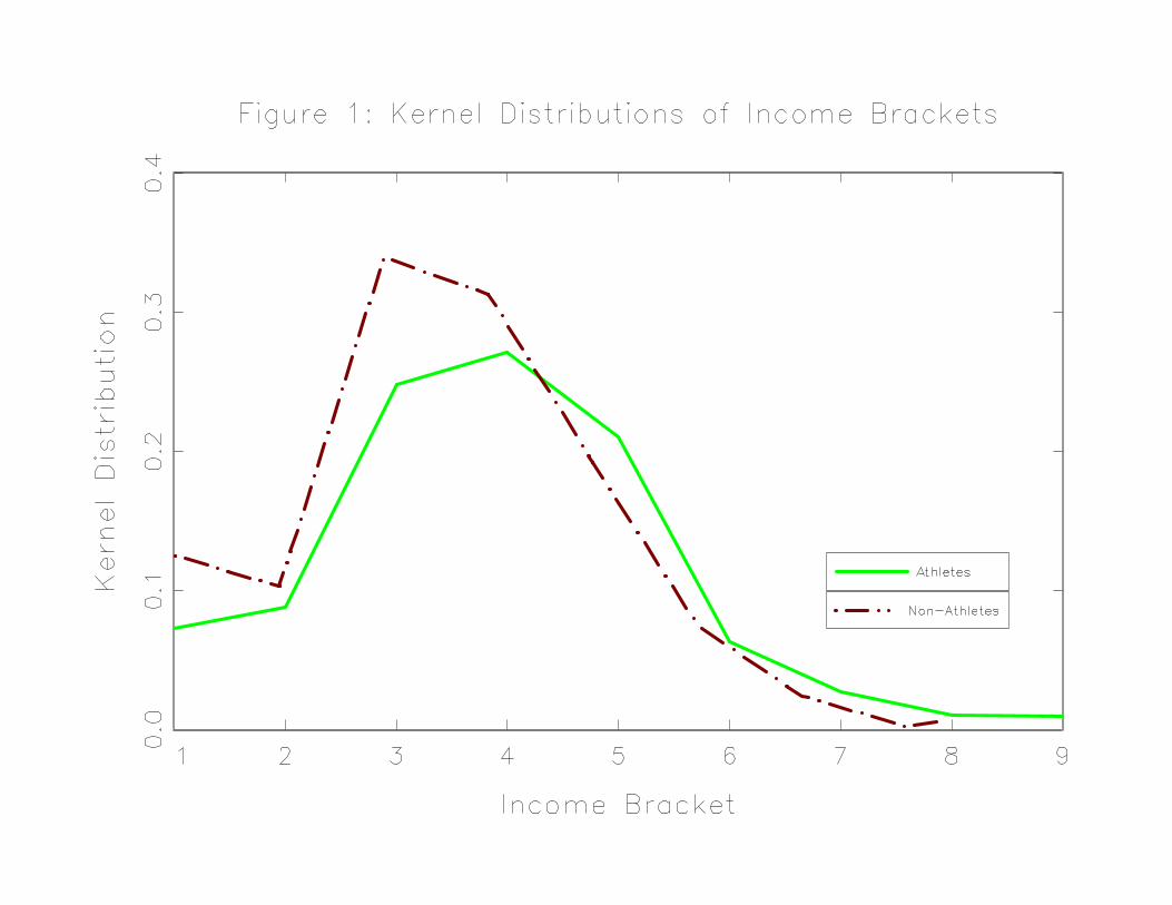
As previously stated, income was reported as a limited dependent variable. The

variable was reported in intervals defined in the following manner: 1 = $1 to $6, 999,

2 = $7, 000 to $9, 999, 3 = $10, 000 to $14, 999, 4 = $15, 000 to $19, 999, 5 = $20, 000

to $24, 999, 6 = $25, 000 to $29, 999, 7 = $30, 000 to $34, 999, 8 = $35, 000 to

$39, 999, and 9 = $40, 000 or more. The distribution of athletes and non-athletes

across income intervals is not identical. Table 2, and Figure 1 show that a slightly

higher percentage of athletes are in the higher income brackets, which most likely

accounts for the slightly higher average wage enjoyed by athletes.

4Only one athlete in the sample was in the highest income bracket and had an occupation listedas “other.” Professional athletes would be expected to be in the highest income bracket and selectan occupation of “other.” Using the preceding criteria, it is unlikely any of the remaining formercollege athletes were professional athletes.

7

In addition to income, Table 1 shows that athletes seem to enjoy a slight ad-

vantage in certain other categories. A higher percentage of athletes completed their

bachelors, masters, and doctoral or professional degrees. Athletes were more likely

to attend a private institution and reported themselves to be on average more driven

and more likely to have a goal to be well-off financially compared to non-athletes.

Neither group had a significant average advantage regarding ACT scores and course

grades, but choice of school and motivation seemed to differ between the two groups.

They were less likely than non-athletes to want to own their own business. Each of

these variables were included as control variables because individuals with a strong

competitive drive, a goal to be financially well-off and a motivation to own their own

business would be expected to earn higher wages, ceteris paribus. In the statistical

analysis to follow, possessing these traits might also make it more likely for an indi-

vidual to play competitive athletics and failure to address these traits could cause a

bias in the coefficient of the ATHLETE variable.

4 Results

4.1 Distribution Tests

Before jumping into the regression, we feel it necessary to perform two distributional

tests. First, we want to establish that the distribution of wages between athletes

and non-athletes are significantly different from one another. Second, we will test

whether the distribution of wages is dependent on athletic participation. Performing

these tests not only strengthen the argument for inclusion of the ATHLETE variable

on the right hand side of our wage regression, but it makes the argument that athletic

participation has a significant impact on the wages of former college students.

There are a number of kernel based tests for the equality of distributions (for

example see Li 1996), however, generally they require that the underlying variable

of interest is continuous in nature. As previously stated, the variable of interest

is ordered and categorical, and thus any kernel based test used requires a kernel

function equipped for discrete data. For this reason, we select the Li, Maasoumi, and

Racine (2004) nonparametric test for equality of distributions with mixed categorical

and continuous data. In our particular case, we are interested in testing whether

8

the probability density function of wages for former college athletes is significantly

different from that of non-athletes. Intuitively, if the null hypothesis is rejected,

then an investigation of why these two distributions are significantly different may be

warranted. With this data, we firmly reject the null hypothesis (p-value = 0.0071).

After establishing a statistical difference between two wage distributions, it is

prudent to test whether explanatory variables have a deterministic effect on the dis-

tribution of wages. The question now becomes, does athletic participation influence

the distribution of wages? If the ATHLETE variable is found to significantly affect

the stability of the conditional probability density function, then a strong argument

can be made as to why this variable should be included in the wage regression. Here

we employ Racine’s (2002) invariance test. This test examines the validity of the

null hypothesis, which states that an underlying distribution does not change with

particular values of a conditioning variable. To test the null, a gradient is constructed

using kernel estimates of the conditional PDF with respect to the conditioning vari-

able of interest, namely the ATHLETE variable. Intuitively, if we reject the null

hypothesis, it is agreed that athletic participation has a statistically significant effect

on the distribution of wages. We find that it does by rejecting the null at the one

percent level of significance (p-value = 0.0005).

4.2 Regression Results

When encountering a situation in which a regression must be estimated using a lim-

ited dependent variable, econometricians often use an ordered logit model.5 However,

using this method not only requires several restrictive assumptions, but it also lim-

its discussion to calculating self determined marginal effects and makes it difficult to

investigate the returns to athletic participation for specific occupations. The nonpara-

metric method we use allows for a more straightforward and flexible interpretation

of the regression coefficients estimated.

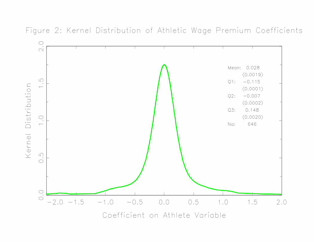
Given the number of parameters obtained from the Generalized Kernel Estimation

procedure, it is tricky to present results. Unfortunately no widely accepted presenta-

tion format exists. Therefore, in Figure 2, we give the mean and the 25th, 50th and

5When estimating an ordered logit model while using the same setup as LC, a coefficient of .269(standard error of .078) for the ATHLETE variable is obtained.

9

75th percentile (labelled Quartile 1, 2 and 3) along with their respective bootstrapped

standard errors as well as a kernel density plot of the coefficients for the athletic par-

ticipation variable for each athlete included in the data set (by definition the athletic

participation coefficient for all non-athletes is zero). Each coefficient represents the

impact on earnings (category) for a one unit increase of the associated independent

variable (in other words, ATHLETE going from 0 to 1).6

One consideration is important in interpreting theATHLETE coefficient. For the

coefficient to be unbiased, ATHLETE must be truly exogenous — implying athletic

status must be randomly assigned. However, it is possible students become athletes

because they are innately motivated and disciplined — qualities that are unobserv-

able but positively correlated with earnings (Duncan and Dunifon 1998). If this is

the case, athletes may earn more not because universities provide value-added, but

because better students become athletes. There are two ways to get at this potential

bias, though each is imperfect. One possibility is to model athletic participation using

a selection rule, and then account for this selectivity in the earnings equation (Willis

and Rosen 1979). For this approach to work one ideally should identify factors that

affect athletic prowess such as height and weight (unavailable in the data) but that

are unrelated to earnings. The problem finding such variables is at best tricky. Partic-

ipating in high school athletics is a possibility, but this variable imperfectly predicts

collegiate athletic participation and besides may be correlated with earnings. A sec-

ond, but also imperfect, approach is to include motivational variables in the original

earnings function in order to hold constant the type “drive” that inspires athletes but

also raises earnings. We adopt this latter approach because the data contain two such

variables: first, a dummy categorical variable indicating whether the respondent rates

himself in the highest 10% in “drive and ambition” (Drive Dummy); and second, a

dummy categorical variable indicating that being “well-off financially is an important

goal” (Well Dummy). Perhaps more importantly, because our true goal is to com-

pare our nonparametric approach to LC, we follow their lead to treat ATHLETE as

exogenous by assuming innate athletic ability to be a god-given talent.

The mean of the coefficients for the ATHLETE variable, 0.028, indicates that

6The mean coefficient values for the remaining regressors are qualitatively similar to the resultsin LC. They are available from the authors upon request.

10

former college athletes are in a 0.028 higher earnings category than non-athletes,

ceteris paribus. Because most income categories represent a $5, 000 wage gap, this

coefficient can be interpreted as approximately a $140 wage benefit. Although quali-

tatively similar, this is smaller than the four percent premium reported by LC. But

the variation in individual wage premiums is more interesting. Less than half the

college athletes actually receive a positive gain. The median of the coefficients (Q2)

is negative, implying a skewed distribution with more than half of former college

athletes actually earning lower wages than non-athletes, ceteris paribus.

Discussing individual variation in parameter values is one of the major benefits

we gain by using the nonparametric technique. Although we found that on average

athletes obtain a wage premium, we were able to show that over half of them did

not. Simply stereotyping all athletes under one estimate is misleading. For exam-

ple, the typical parametric approach, such as used by LC suggest that athletes earn

higher wages than non-athletes, ceteris paribus. If individuals choosing whether or

not to participate in college athletics take this information as given, it could affect

their decision making. Given the positive coefficient on ATHLETE found by LC,

individuals may decide to participate in sports because they believe that their wages

will rise in the future. Similarly, universities may opt for sports programs believing

that individual students necessarily benefit. However, our result shows that the wage

premium is not uniform across athletes. Although some athletes enjoy large wage

benefits, others earn less than non-athletes. Thus, for students, the more appropriate

question is not whether to participate in sports, but the more specific question should

be, if an individual participates in a sport, in which occupations will that individual

most likely earn a wage premium over non-athletes?

Table 3 shows the estimates on the ATHLETE variable for four job categories;

as well as for a fifth category depicting all other occupations combined. The four

occupations, high school teaching, business, military, and manual labor are ones with

a significant number of former athletes (arbitrarily chosen as those occupations with

at least 35 athletes). For the latter three occupations (business, military, and manual

labor), the mean and median are positive, indicating that a wage premium is present

for a majority of athletes in those occupations. Intuitive arguments could be made

that skills obtained or improved during athletic participation would justify wage

11

premiums in these occupations. Teamwork skills and an enhanced competitive drive

to succeed could be useful in the business world. Physical strength and other athletic

attributes may make manual laborers and military professionals more productive at

their jobs, justifying higher wages. The ability to apply strategic thinking and adjust a

particular strategy during a game may be particularly important while using military

tactics, may be important during a business negotiation, or may be important when

operating as a team to perform some physical task. Many of these reasons apply to

the conglomerate occupation, as well.

Althoughmost job categories were associated with wage premiums, the high school

teaching occupation was not. In teaching, a majority of former college athletes earn

lower wages, ceteris paribus, as compared to non-athletes in this category. Although

we will shortly discuss potential explanations of this observation, a wage premium

can affect occupational choice. Specifically one would expect former athletes to enter

jobs where they earn high wages and shy away from jobs where they do not. But this

is not the case for athletes.

Table 4 reports the results of a logit model where the binary dependent variable,

HSTEACHER, takes a value one if an individual reported high school teaching as

an occupation, zero otherwise. In this data, former college athletes were found to

be more likely to select high school teaching as an occupation, despite earning lower

wages. Similarly, we found this result to hold on population subsamples such as for

African Americans. Several arguments can be levied to explain this behavior, but no

evidence in the data clearly supports any claim in particular.

First, becoming a teacher may be driven by a non-pecuniary desire for upward

social mobility. Falk, Falkowski and Lyson (1981), and Schwarzweller and Lyson

(1978) report that the highly respected teaching profession is a source of upward social

and professional intergenerational mobility for rural whites and African Americans,

especially during the 1970s. If athletes are more likely to be motivated to improve

their lives, they may have viewed a teaching profession as a means to improve their

status in life. The teaching occupation generally provides fewer barriers to entry and

as a governmental organization is not allowed by law to discriminate against any

particular group. The accessibility and attractiveness of teaching may explain why

African American former college athletes are more likely to choose this profession.

12

Several other theories are worth mentioning. If athletics fosters an increased

affection for a school, then an athlete may wish to return to his high school to work.

Athletes may also wish to pursue coaching. Because high school teachers often serve

as coaches, this desire may be reflected in their occupational choice decision. Even

if former athletes choosing this profession realize they will be expected to earn lower

average wages, the increased utility generated by coaching may offset any monetary

losses.

Regardless of the reason(s) for becoming teachers, a relatively large supply of for-

mer athletes could exert downward wage pressure in the teaching occupation. If a

labor market is inordinately supplied with individuals possessing similar traits, then

that group’s wages could be lower than comparably skilled workers in other mar-

kets. For example, if many former athletes are trying to become physical education

teachers, then the wages of physical education teachers could be lower than other

teachers.

5 Conclusion

Estimating the impact of individual behavior is an important aspect of social research.

Often outcome can be measured in monetary units. When this is the case, one can

estimate an earnings function to determine how an individual’s actions affect his

or her earnings. In most cases, parametric models are used. However, parametric

models have certain restrictions regarding functional form. In addition, they are

usually specified in ways to yield a single coefficient estimate.

One such example is the effect of a student’s participation in college athletics on

earnings years after leaving college, a topic not well studied because of the paucity of

data. However, in one such study Long and Caudill (1991) find that college athletes

earn about a 4% positive return from collegiate sports. Because of certain data

restrictions (a categorical dependent variable) they use Nelson’s (1976) maximum

likelihood procedure, but as with most such parametric procedures that paper limits

itself to obtaining a single coefficient without exploring how robust their findings are

across the population.

This paper reexamines the issue using a new technique. The Li-Racine General-

ized Kernel Estimation procedure is able to assess the impact of an exogenous variable

13

within a model containing an ordered categorical dependent variable along with con-

tinuous, unordered, and ordered categorical regressors. Of course, the beauty of the

technique is its ability to estimate coefficients for each individual so that one can

assess the impact of athletic participation across the sample.

This paper examines the CIRP data. Unlike past studies, we find that the wage

premiums associated to former college athletes are not uniform. Rather, athletes earn

between a 1.5 and 9 percent average wage premium in business, manual labor and

military careers, but nonetheless enter teaching occupations with a higher probability

than non-athletes despite facing an average wage deficiency of 8 percent. Whereas

wage premiums in the former three occupations conform to the human capital type

matching models of occupational choice, the latter result regarding teaching are con-

sistent with non-pecuniary incentives explaining occupational choice. This latter

result regarding non-pecuniary motivators imply broader implications than usually

inferred from typical economics models based solely on pecuniary factors.

Institutions of higher education need good reasons when deciding how to spend

limited funds. If a financial value can be linked to athletics, a stronger argument

may be employed to justify investment in athletics programs. This paper argues

that financial benefits are not uniform to all individuals who play sports. On average

athletes receive a modest return and go into occupations where they do best. But this

is not the case for all collegiate athletes. Almost 10% enter teaching, an occupation

with an especially low wage for athletes. Further, a good 50% do no better than the

college population at large.

14

References

[1] Aitchison, J. and C. G. G. Aitken (1976). “Multivariate Binary Discrimination

by the Kernel Method,” Biometrika, 63, 413-20.

[2] Astin, A. (1982). Minorities in American Higher Education, Jossey-Bass, San

Francisco.

[3] Duncan, G. J. and R. Dunifon (1998). “‘Soft-Skills’ and Long-Run Labor Market

Success,” Research in Labor Economics, 17, 123-49.

[4] Ewing, B. (1995). “High School Athletics and the Wages of Black Males,” Review

of Black Political Economy, 24, 65-78.

[5] Falk, W. W., C. Falkowski,and T. A. Lyson (1981). “Some Plan to Become

Teachers’: Further Elaboration and Specification,” Sociology of Education, 54,

64-9.

[6] Hall, P., J. Racine and Q. Li (2004). “Cross-Validation and the Estimation of

Conditional Probability Densities,” Journal of The American Statistical Associ-

ation, 99, 1015-26.

[7] Kniesner, T. and Q. Li (2002). “Nonlinearity in Dynamic Adjustment: Semipara-

metric Estimation of Panel Labor Supply,” Empirical Economics, 27, 131-48.

[8] Li, Q. (1996). “Nonparametric Testing of Closeness between Two Unknown Dis-

tribution Functions,” Econometric Reviews, 15, 261-74.

[9] Li, Q. and D. Ouyang (2005). “Uniform Convergence Rate of Kernel Estimation

with Mixed Categorical and Continuous Data,” Economics Letters, 86, 291-6.

[10] Li, Q., E. Maasoumi and J. Racine (2004). “A Nonparametric Test for the Equal-

ity of Distributions With Mixed Categorical and Continuous Data,” manuscript,

Syracuse University.

[11] Li, Q. and J. Racine (2003). “Nonparametric Estimation of Distributions with

Categorical and Continuous Data,” Journal of Multivariate Analysis, 86, 266-92.

15

[12] Li, Q. and J. Racine (2004). “Cross-Validated Local Linear Nonparametric Re-

gression,” Statistica Sinica, 14, 485-512.

[13] Li, Q. and J. Racine (2005). Nonparametric Econometrics: Theory and Practice,

Princeton, Princeton University Press, (forthcoming).

[14] Long, J. and S. Caudill (1991). “The Impact of Participation in Intercollegiate

Athletics on Income and Graduation,” Review of Economics and Statistics, 73,

525-31.

[15] N c°, Nonparametric software by Jeff Racine

(http://www.economics.mcmaster.ca/racine/).

[16] NCAA (2004). “Revenues and Expenses of Intercollegiate Athletics Programs”

and “NCAA Facts,” (http://www.ncaa.org).

[17] Nelson, F. (1976). “On a General Computer Algorithm for the Analysis of Models

with Limited Dependent Variables,” Annals of Economic and Social Measure-

ment, 493-509.

[18] Pagan, A. and A. Ullah (1999). Nonparametric Econometrics, Cambridge Uni-

versity Press, Cambridge.

[19] Racine, J. (2002). “A Consistent Nonparametric Distributional Invariance Test,”

manuscript, Syracuse University.

[20] Racine, J. and Q. Li (2004). “Nonparametric Estimation of Regression Functions

with Both Categorical and Continuous Data,” Journal of Econometrics, 119, 99-

130.

[21] Schwarzweller, H. K. and T. A. Lyson (1978). “Some Plan to Become Teachers:

Determinants of Career Specification among Rural Youths in Norway, Germany,

and the United States,” Sociology of Education, 51, 29-43.

[22] Wang, M. C. and J. Van Ryzin (1981). “A Class of Smooth Estimators for

Discrete Estimation,” Biometrika, 68, 301-9.

16

[23] Willis, R. J. and S. Rosen (1979). “Education and Self-Selection,” Journal of

Political Economy, 87: S7-36.

17

Table 1: Descriptive Statistics for CIRP DataVariable Non-Athletes (Nn = 3563) Athletes (Na = 646)

Mean Standard Deviation Mean Standard DeviationIncome (Bracket) 4.685 1.605 4.854 1.516Income (in Dollars) 18025 19270ACT Score 23.030 3.889 23.889 3.785African American 0.127 0.333 0.178 0.383Bachelors Degree 0.521 0.500 0.576 0.495Drive Dummy 0.280 0.449 0.348 0.477Family Dummy 0.267 0.443 0.305 0.461Firm Size 4.040 1.756 4.141 1.722Grades 4.459 1.107 4.430 1.030Married 0.502 0.500 0.506 0.500Masters Degree 0.143 0.350 0.156 0.363Number of Children 0.385 0.728 0.364 0.708Part-Time Employed 0.068 0.251 0.050 0.217Ph.D. or Professional Degree 0.086 0.281 0.105 0.307Private 0.578 0.494 0.738 0.440Runbus 0.165 0.371 0.149 0.356School Enrollment 5.374 1.871 4.717 1.650Self Employed 0.054 0.225 0.037 0.189Veteran 0.029 0.169 0.006 0.079Well Dummy 0.144 0.351 0.161 0.368NOTES: Descriptions of each variable are provided in the Appendix A and income brackets are described in Table 2.

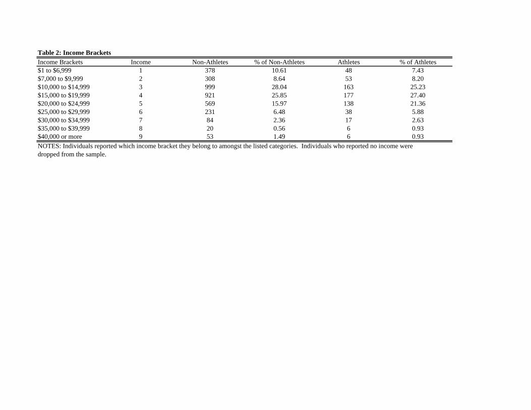
Table 2: Income BracketsIncome Brackets Income Non-Athletes % of Non-Athletes Athletes % of Athletes$1 to $6,999 1 378 10.61 48 7.43$7,000 to $9,999 2 308 8.64 53 8.20$10,000 to $14,999 3 999 28.04 163 25.23$15,000 to $19,999 4 921 25.85 177 27.40$20,000 to $24,999 5 569 15.97 138 21.36$25,000 to $29,999 6 231 6.48 38 5.88$30,000 to $34,999 7 84 2.36 17 2.63$35,000 to $39,999 8 20 0.56 6 0.93$40,000 or more 9 53 1.49 6 0.93NOTES: Individuals reported which income bracket they belong to amongst the listed categories. Individuals who reported no income were dropped from the sample.

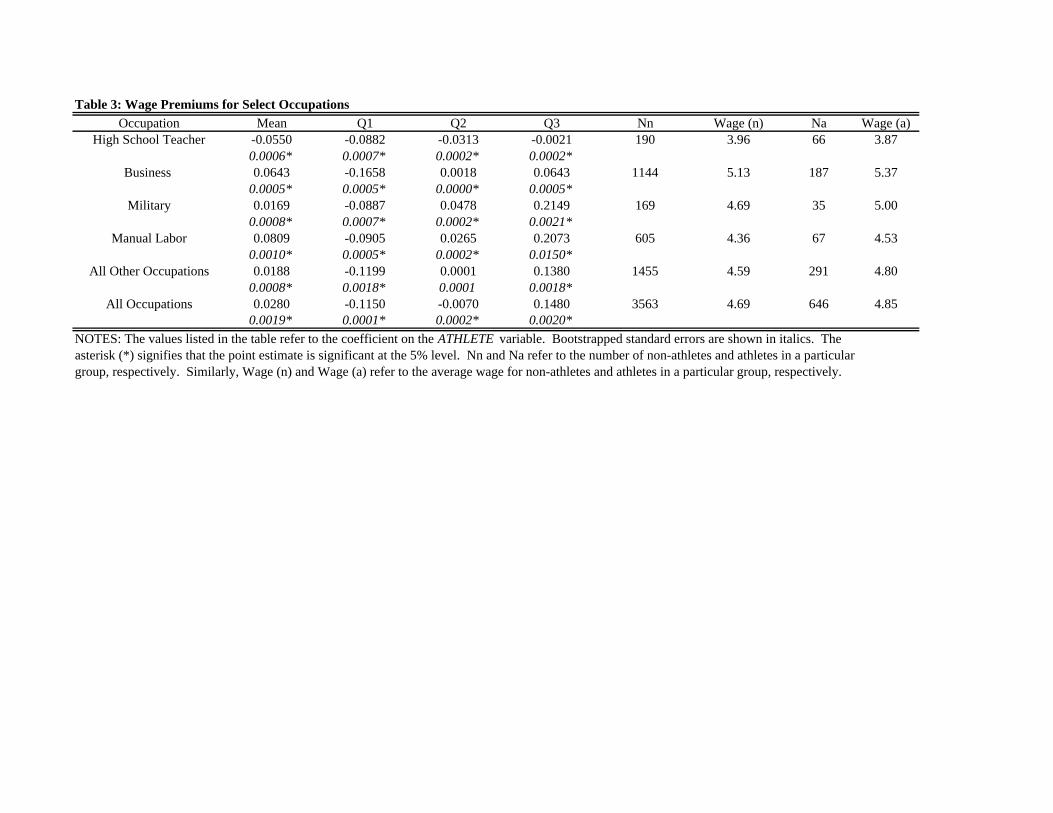
Table 3: Wage Premiums for Select OccupationsOccupation Mean Q1 Q2 Q3 Nn Wage (n) Na Wage (a)

High School Teacher -0.0550 -0.0882 -0.0313 -0.0021 190 3.96 66 3.870.0006* 0.0007* 0.0002* 0.0002*

Business 0.0643 -0.1658 0.0018 0.0643 1144 5.13 187 5.370.0005* 0.0005* 0.0000* 0.0005*

Military 0.0169 -0.0887 0.0478 0.2149 169 4.69 35 5.000.0008* 0.0007* 0.0002* 0.0021*

Manual Labor 0.0809 -0.0905 0.0265 0.2073 605 4.36 67 4.530.0010* 0.0005* 0.0002* 0.0150*

All Other Occupations 0.0188 -0.1199 0.0001 0.1380 1455 4.59 291 4.800.0008* 0.0018* 0.0001 0.0018*

All Occupations 0.0280 -0.1150 -0.0070 0.1480 3563 4.69 646 4.850.0019* 0.0001* 0.0002* 0.0020*

NOTES: The values listed in the table refer to the coefficient on the ATHLETE variable. Bootstrapped standard errors are shown in italics. The asterisk (*) signifies that the point estimate is significant at the 5% level. Nn and Na refer to the number of non-athletes and athletes in a particulargroup, respectively. Similarly, Wage (n) and Wage (a) refer to the average wage for non-athletes and athletes in a particular group, respectively.

Table 4: Logit Model -- Determinants of Becoming a High School TeacherVariable Estimate Standard ErrorIntercept -3.097 0.740ACT Score -0.059 0.026*African American -0.040 0.260Bachelor's Degree 2.424 0.434*Drive Dummy 0.154 0.175Firm Size -0.130 0.051*Grades 0.128 0.092High School Athlete 0.846 0.172*Major1 -0.878 0.465*Major10 -1.094 0.762Major11 -1.455 0.544*Major2 -1.094 0.238*Major3 -0.851 0.294*Major4 -3.336 0.477*Major5 -3.308 0.732*Major6 -1.263 0.298*Major7 -1.937 0.741*Major8 -14.891 561.8Major9 -1.694 0.243*Married 0.122 0.174Master's Degree 2.467 0.466*Number of Children -0.181 0.137Ph.D. or Professional Degree 0.257 0.743Private 0.110 0.226Runbus -0.938 0.304*School Enrollment 0.020 0.057Veteran -0.178 0.547NOTES: The dependent variable in this logit regression is the High School Teaching Occupation. See Appendix A for descrptions of each of the variables. See Appendix C for the definitions of theacademic fields constituting each major. The asterisk (*) signifies that the estimate is significant at the 5% level.

Appendix A: Variable DefinitionsVariable MeaningACT Score Score on American College Test (range from 9 to 30)African American 1 if African American, 0 otherwiseAthlete 1 if earned a varsity letter in college, 0 otherwiseBachelor's Degree 1 if holds bachelors degree, 0 otherwiseBusiness 1 if individual reported occupation as business clerical, business management

or business sales, 0 otherwiseDrive Dummy 1 if individual rates themselves in the highest 10 percent to “drive to achieve”Family Dummy 1 if an individual reported that having a family was an important goal, 0 otherwiseFirm Size Number of employees in firm individual works for, reported in categoriesGrades Self reported average college grades (A to F scale)Manual Labor 1 if individual reported occupation as skilled, semi-skilled or unskilled labor, 0

otherwiseMAJXX Represents various college majors (See Appendix C)Married 1 if married, 0 otherwiseMasters Degree 1 if holds masters degree, 0 otherwiseMilitary 1 if individual reported occupation as military career, 0 otherwiseNumber of Children Number of offspringOCCXX Represents various occupations (see occupations list)Part-Time Employed 1 if an individual was employed part-time, 0 otherwisePh.D. or Professional degree 1 if holds Ph.D. or advanced professional degree, 0 otherwisePrivate 1 if college attended was a privately owned institution, 0 otherwiseRunbus 1 if an individual reported that owning their own business was a goal, 0 otherwiseSchool Enrollment Total enrollment of college, reported in categoriesSelf Employed 1 if individual was self-employed, 0 otherwiseTeacher 1 if individual reported occupation as secondary or elementary teacherVeteran 1 if military veteran, 0 otherwiseWell Dummy 1 if “being well off financially” is an important goal, 0 otherwise

Appendix B: Definitions of OccupationsOCC1: 1OCC2: 15, 25, 29, 30, 31, 40OCC 3: 43 thru 47OCC 4: 17OCC 5: 23, 28, 35, 37OCC 6: 6, 7, 8OCC 7: 2, 4, 27, 41OCC 8: 3OCC 9: 11, 13, 34, 36OCC10: 14, 18OCC 11: 19, 22, 24, 26OCC 12: 12OCC 13: 9, 10OCC 14: 16, 21OCC 15: 42OCC 16: 5

1 Accounting 25 Lawyer2 Actor/Entertainer 26 Military Service3 Architect 27 Musician4 Artist 28 Nurse5 Business Clerical 29 Optometrist6 Business Management 30 Pharmacist7 Proprietor 31 Physician8 Business Sales 32 School Counselor9 Clergy 33 School Principal

10 Other Religious 34 Scientific Researcher11 Psychologist 35 Social Worker12 College Teacher 36 Statistician13 Computer Programmer 37 Therapist14 Conservationist or Forester 38 Teacher (Elementary)15 Dentist 39 Teacher (High School)16 Dietician/Home economics 40 Veterinarian17 Engineer 41 Writer/Journalist18 Farmer/Rancher 42 Skilled Trades/ Skilled Manual Labor19 Foreign Service Worker 43 Other20 Homemaker 44 Unskilled Worker/Unskilled Manual Labor21 Interior Decorator 45 Semi-Skilled Worker/Semi-Skilled 22 Interpreter Manual Labor23 Lab Technician 46 Other Occupation24 Law Enforcement 47 Unemployed

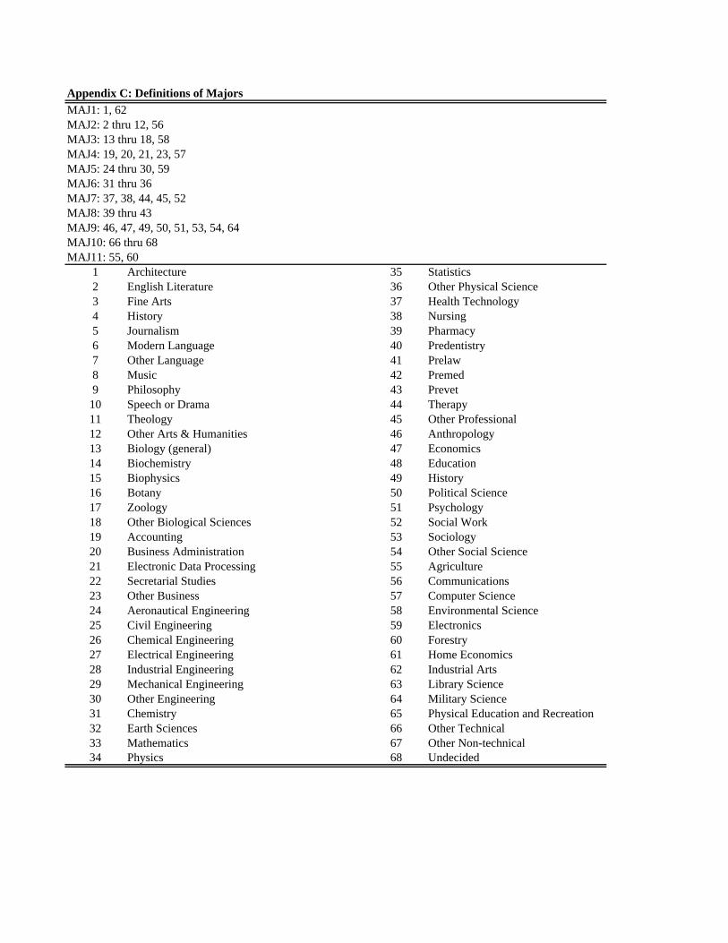
Appendix C: Definitions of MajorsMAJ1: 1, 62MAJ2: 2 thru 12, 56MAJ3: 13 thru 18, 58MAJ4: 19, 20, 21, 23, 57MAJ5: 24 thru 30, 59MAJ6: 31 thru 36MAJ7: 37, 38, 44, 45, 52MAJ8: 39 thru 43MAJ9: 46, 47, 49, 50, 51, 53, 54, 64MAJ10: 66 thru 68MAJ11: 55, 60

1 Architecture 35 Statistics2 English Literature 36 Other Physical Science3 Fine Arts 37 Health Technology4 History 38 Nursing5 Journalism 39 Pharmacy6 Modern Language 40 Predentistry7 Other Language 41 Prelaw8 Music 42 Premed9 Philosophy 43 Prevet

10 Speech or Drama 44 Therapy11 Theology 45 Other Professional12 Other Arts & Humanities 46 Anthropology13 Biology (general) 47 Economics14 Biochemistry 48 Education15 Biophysics 49 History16 Botany 50 Political Science17 Zoology 51 Psychology18 Other Biological Sciences 52 Social Work19 Accounting 53 Sociology20 Business Administration 54 Other Social Science21 Electronic Data Processing 55 Agriculture22 Secretarial Studies 56 Communications23 Other Business 57 Computer Science24 Aeronautical Engineering 58 Environmental Science25 Civil Engineering 59 Electronics26 Chemical Engineering 60 Forestry27 Electrical Engineering 61 Home Economics28 Industrial Engineering 62 Industrial Arts29 Mechanical Engineering 63 Library Science30 Other Engineering 64 Military Science31 Chemistry 65 Physical Education and Recreation32 Earth Sciences 66 Other Technical33 Mathematics 67 Other Non-technical34 Physics 68 Undecided