Do commodity prices affect exchange rate differently in …€¦ · · 2017-09-27In this thesis...
206
Do commodity prices affect exchange rate differently in developed and developing countries? A comparative study of OECD and ASEAN Thi Anh Thu Tran Thesis submitted in fulfillment of the requirements for the degree of Master of Business (by research) Faculty of Business and Law Swinburne University of Technology 2016
Transcript of Do commodity prices affect exchange rate differently in …€¦ · · 2017-09-27In this thesis...

Do commodity prices affect exchange rate
differently in developed and developing countries?
A comparative study of OECD and ASEAN
Thi Anh Thu Tran
Thesis submitted in fulfillment of the
requirements for the degree of
Master of Business (by research)
Faculty of Business and Law
Swinburne University of Technology
2016

i
Abstract
In this thesis are compared the relationship between exchange rate and commodity
prices between OECD and ASEAN commodity-exporting countries. Based on the
similarity between OECD and ASEAN in terms of demographics, commodity export,
financial markets, economic performance, and development prospects, the thesis makes
some predictions for the relationship between real exchange rate and real commodity
prices in ASEAN developing commodity-exporting countries when they reach
“developed country” status. Moreover, this thesis gives some policy implications for
these countries in the management of commodity prices and exchange rate during the
transition period.
The relationship between real exchange rate and real commodity prices in the two
groups of countries is examined in terms of cointegration, elasticity of real exchange
rate to real commodity prices, and Granger causality by employing both time-series and
panel-data techniques. The test results indicate that there is a considerable difference in
this relationship between developed and developing commodity-exporting countries.
Specifically, in OECD commodity-exporting countries, real commodity prices and real
exchange rate move together in the same direction in the long run and changes in real
commodity prices will lead to responses of real exchange rate in order to re-establish
the equilibrium. Meanwhile, in ASEAN commodity-exporting countries, real
commodity prices and real exchange rate do not seem to have long-term relationship.
This thesis also gives explanations for the differences in the relationship between
OECD and ASEAN commodity-exporting countries: differences in exchange rate
regimes, ability to expand the natural-resource sector, and level of financial openness
between the two groups of countries. It is expected that on the way to achieving the
“developed country” status, the three factors of ASEAN commodity-exporting countries
would be likely to evolve toward the trend currently seen in OECD commodity-
exporting countries and the relationship between real commodity prices and real
exchange rate would become stronger.

ii
However, a stronger relationship between real exchange rate and real commodity prices
might be harmful to the economy, especially when the financial system is
underdeveloped. To reduce the negative effects of the relationship on the overall
economy in the transition period, this thesis suggests that ASEAN commodity-
exporting countries smooth their government spending, diversify export commodities
and diversify their economies.
iii
Acknowledgements
Foremost, I would like to say thank you to my supervisory team. My Principal
Coordinating Supervisor, Dr. Omar Bashar has provided me with a foundation upon
which I built my journey and endless amounts of encouragement as I worked toward
completion. He was always there – whenever and whatever I needed – with academic
advice and guidance as well as personal care and support. He challenged me to go
deeper and further throughout his comments and feedback on my work. My Co-
Coordinating Supervisor, A/Prof Malcolm Abbott, with his immense knowledge and
research experience, has always given me valuable advice when I had trouble with my
thesis. I am blessed to have had A/Prof Malcolm to work with.
I would like to thank my review panel: Dr. Chee Jin Yap, Dr. Mark Bowden and A/Prof
Steven Greenland for their insightful comments and encouragement. Furthermore, I
would like to thank Vincent J. Bodart for giving me access to the data of REER. His
kindly support is really valuable to me.
Swinburne University of Technology has fostered my development and my learning.
Again, I am grateful for the support I have received from the Faculty of Business and
Law, and to Swinburne Research in providing me training and support services. I would
especially like to thank Anne Cain, Nadine White, Elena Verezub, and Melissa Cogdon
for all of their support, advice and guidance throughout my journey.
Lastly, I would like to dedicate this thesis to my husband Huan Nguyen Tuong, my
parents, Loc Tran Tan and Be Nguyen Thi, my brother Liem Tran Tan, and my parents-
in-law, Lai Nguyen Dinh and Loc Tran Thi Xuan. They encouraged and supported me
and were always there with their love when I needed it. I could not have completed this
thesis without them.

iv
Declaration
This thesis:
- Contains no material that has been accepted for the award to the candidate of
any other degree or diploma, except where due reference is made in the text of
the examinable outcome;
- To the best of the candidate’s knowledge contains no material previously
published or written by another person except where due reference is made in
the text of the examinable outcome;
- This thesis is 50,709 words in length exclusive of bibliography and appendices;
and
- Ian M. Hoffman, Ph.D. edited this thesis. The editing addressed only style and
grammar and not its substantive content.
Thi Anh Thu Tran
Jan 20th, 2016

v
Table of contents
Abstract .............................................................................................................................. i
Acknowledgement............................................................................................................ iii
Declaration ....................................................................................................................... iv
Table of contents ............................................................................................................... v
List of abbreviations ....................................................................................................... viii
List of tables ...................................................................................................................... x
List of figures ................................................................................................................. xiii
1.1 Background and motivation ................................................................................. 1
1.2 Aims and research questions ................................................................................ 3
1.3 Contributions........................................................................................................ 4
1.4 Theoretical link between real exchange rate and real commodity prices ............ 5
1.5 Thesis structure .................................................................................................... 8
1.6 Summary .............................................................................................................. 9
2.1 The OECD ......................................................................................................... 10
2.2 The ASEAN ....................................................................................................... 14
2.3 Why pick up OECD and ASEAN ...................................................................... 17
2.4 Commodity-exporting countries ........................................................................ 20
2.4.1 OECD commodity-exporting countries ....................................................... 20
2.4.2 ASEAN commodity-exporting countries .................................................... 33
2.5 Summary ............................................................................................................ 44
3.1 Non-oil commodity prices and exchange rate ................................................... 46
3.1.1 Non-oil commodity prices and exchange rate in developed countries ........ 46
3.1.2 Non-oil commodity prices and exchange rate in developing countries ...... 50
3.1.3 Non-oil commodity prices and exchange rate in both developed and
developing countries ............................................................................................... 53

vi
3.2 Oil prices and exchange rate .............................................................................. 56
3.2.1 Oil prices and exchange rate in developed countries .................................. 56
3.2.2 Oil prices and exchange rate in developing countries ................................. 58
3.2.3 Relationship between oil prices and exchange rate in both developed and
developing countries ............................................................................................... 62
3.3 Summary ............................................................................................................ 64
4.1 Variables ............................................................................................................ 66
4.2 Data source......................................................................................................... 68
4.2.1 Selection of countries .................................................................................. 68
4.2.2 Commodity prices ....................................................................................... 70
4.2.3 Exchange rate .............................................................................................. 78
4.2.4 Real interest rate .......................................................................................... 86
4.3 Methodology ...................................................................................................... 87
4.3.1 Time-series technique .................................................................................. 87
4.3.2 Panel-data technique .................................................................................... 97
4.4 Summary .......................................................................................................... 110
5.1 Test results ....................................................................................................... 112
5.1.1 Individual countries ................................................................................... 112
5.1.2 Groups of countries ................................................................................... 132
5.2 Analysis of test results ..................................................................................... 141
5.2.1 OECD ........................................................................................................ 141
5.2.2 ASEAN ...................................................................................................... 142
5.3 Discussion ........................................................................................................ 143
5.4 Summary .......................................................................................................... 152
6.1 Development plans of ASEAN commodity-exporting countries .................... 153
6.1.1 Development plans of ASEAN ................................................................. 153
6.1.2 Development plans of individual ASEAN commodity-exporting countries
157

vii
6.2 Predictions for the relationship between exchange rate and real commodity
prices in ASEAN commodity-exporting countries ................................................... 162
6.3 Policy implications for ASEAN commodity-exporting countries in their
transition period ........................................................................................................ 165
6.3.1 Smooth spending ....................................................................................... 168
6.3.2 Diversifying export commodities .............................................................. 169
6.3.3 Diversifying economies ............................................................................. 169
6.4 Summary .......................................................................................................... 170
7.1 Summary of the thesis ...................................................................................... 171
7.2 Limitations of the thesis ................................................................................... 172
7.3 Future research ................................................................................................. 174
7.4 Summary .......................................................................................................... 175
References

viii
List of abbreviations
ADF Augmented Dickey – Fuller
AIA ASEAN Investment Area
ARDL Auto-regressive distributed lag
ASEAN Association of Southeast Asian Nations
BOG Bank of Greece
CLMV Cambodia, Laos, Myanmar and Vietnam
CPI Consumer price index
DOLS Dynamic ordinary least squares
FDI Foreign direct investment
FMOLS Fully modified ordinary least squares
GDP Gross domestic product
GMM Generalized method of moments
HS Harmonized system
IFS International financial statistics
IGA Investment guarantee agreement
IMF International Monetary Fund
LLC Levin, Lin, & James Chu
LRE Long-run elasticity
LSDV Least square dummy variables
LSDVC Bias-corrected least square dummy variables
MUV Manufacturers unit value
MYR Malaysia Ringgit
NCOMP Nominal country-specific commodity prices
NZD New Zealand Dollar
OECD Organization for Economic Cooperation and Development
OLS Ordinary least squares
PP Philips – Perron

ix
PVAR Panel vector autoregression
RCOMP Real commodity prices
REER Real effective exchange rate
RIR Real interest rate
SAARC South Asian Association for Regional Cooperation
SDR Special drawing right
SMEs Small and medium-size enterprises
UNCTAD United Nations Conference on Trade and Development
UN COMTRADE United Nations Commodity Trade Statistics
USD United States Dollar
VAR Vector autoregressive
VEC Vector error correction

x
List of tables
Table 2.1 – Top 15 export commodities in OECD 2007-2012 ....................................... 13
Table 2.2 – Top 15 export commodities in ASEAN 2007-2012 ..................................... 16
Table 2.3 – Top 20 export commodities in Australia 2000-2013 ................................... 21
Table 2.4 – Top 20 export commodities in Canada 2000-2013 ...................................... 23
Table 2.5 – Top 20 export commodities in Iceland 2000-2013 ...................................... 25
Table 2.6 – Top 20 export commodities in New Zealand 2000-2013 ............................ 27
Table 2.7 – Top 20 export commodities in Norway 2000-2013 ..................................... 30
Table 2.8 – Top 20 export commodities in Greece 2000-2013 ....................................... 32
Table 2.9 – Top 20 export commodities in Brunei 2000-2013 ....................................... 34
Table 2.10 – Top 20 export commodities in Malaysia 2000-2013 ................................. 37
Table 2.11 – Top 18 export commodities in Myanmar 2000-2013 ................................ 39
Table 2.12 – Top 20 export commodities in Thailand 2000-2013 .................................. 41
Table 2.13 – Top 20 export commodities in Vietnam 2000-2013 .................................. 43
Table 3.1 – Long-run elasticity of exchange rate to non-oil commodity prices in
developed countries ................................................................................................. 49
Table 3.2 – Long-run elasticity of exchange rate to non-oil commodity prices in
developing countries ............................................................................................... 53
Table 3.3 – Long-run elasticity of exchange rate to non-oil commodity prices in both
developed and developing countries ....................................................................... 55
Table 3.4 – Long-run elasticity of exchange rate to oil prices in developed countries... 58

xi
Table 3.5 – Long-run elasticity of exchange rate to oil prices in developing countries . 61
Table 3.6 – Long-run elasticity of exchange rate to oil prices in both developed and
developing countries ............................................................................................... 64
Table 4.1 – Average share of primary commodities on total exports in ASEAN
countries 1995-2005 ................................................................................................ 68
Table 4.2 – Average share of primary commodities on total exports in OECD countries
1995-2005 ............................................................................................................... 68
Table 4.3 – 45 commodities with HS2007 codes used in the UN Comtrade database ... 73
Table 4.4 – Top five commodity exports by countries in the period 1995-2005 ............ 75
Table 4.5 – The export weights of 21 primary commodities by countries (by percentage)
................................................................................................................................. 76
Table 5.1 – Unit root tests for REER, RCOMP and RIR – individual OECD countries
............................................................................................................................... 113
Table 5.2 – Unit root tests for REER, RCOMP and RIR – individual ASEAN countries
............................................................................................................................... 115
Table 5.3 – Lag length for Johansen (1988) cointegration test between REER and
RCOMP ................................................................................................................. 117
Table 5.4 – Johansen (1988) cointegration tests for REER and RCOMP – OECD
countries ................................................................................................................ 118
Table 5.5 – Johansen (1988) cointegration tests for REER and RCOMP – ASEAN
countries ................................................................................................................ 119
Table 5.6 – Cointegration equations – OECD countries ............................................... 120
Table 5.7 – Cointegration equations – ASEAN countries ............................................ 120
Table 5.8 – Granger causality test (VEC model) – OECD countries............................ 121
Table 5.9 – Granger causality test proposed by Toda and Yamamoto (VAR model) –
OECD countries .................................................................................................... 122

xii
Table 5.10 – Granger causality test (VEC model) – ASEAN countries ....................... 123
Table 5.11 – Granger causality test proposed by Toda and Yamamoto (VAR model) –
ASEAN countries .................................................................................................. 124
Table 5.12 – Residual serial correlation Lagrange multiplier test for VEC models ..... 125
Table 5.13 – Residual serial correlation Lagrange multiplier test for VAR models..... 125
Table 5.14 – Panel unit root tests for REER, RCOMP and RIR ................................... 134
Table 5.15 – Pedroni (1999) Panel Cointegration Test for REER and RCOMP – 6
OECD countries .................................................................................................... 135
Table 5.16 – Pedroni (1999) Panel Cointegration Test for REER and RCOMP – 6
ASEAN countries .................................................................................................. 136
Table 5.17 – Granger causality test (panel VEC model) – 6 OECD countries ............. 137
Table 5.18 – Residual serial correlation Lagrange multiplier (LM) test for panl VEC
model ..................................................................................................................... 137
Table 5.19 – Granger causality test proposed by Toda and Yamamoto (VAR model) – 6
ASEAN countries .................................................................................................. 138
Table 5.20 – Residual serial correlation Lagrange multiplier test for VAR model ...... 138
Table 5.21 – Exchange rate regimes ............................................................................. 145
Table 5.22 – KAOPEN index........................................................................................ 150

xiii
List of figures
Figure 2.1 – GDP per capita of OECD, ASEAN and others, 2000-2012 ....................... 11
Figure 2.2 – International trade in goods of OECD and ASEAN 2000-2012................. 12
Figure 2.3 – Commodity export and total export of OECD 1995-2013 ......................... 13
Figure 2.4 – Exchange rate arrangements in OECD 2003-2013 ..................................... 14
Figure 2.5 – Commodity export and total export of ASEAN 1995-2013 ....................... 15
Figure 2.6 – Exchange rate arrangements in ASEAN 2003-2013 .................................. 16
Figure 2.7 – GDP per capita of Australia, Canada, Iceland, New Zealand, ................... 21
Figure 4.1 – REER and RCOMP in Australia ................................................................ 80
Figure 4.2 – REER and RCOMP in Canada ................................................................... 80
Figure 4.3 – REER and RCOMP in Iceland ................................................................... 81
Figure 4.4 – REER and RCOMP in New Zealand .......................................................... 81
Figure 4.5 – REER and RCOMP in Norway .................................................................. 82
Figure 4.6 – REER and RCOMP in Greece .................................................................... 82
Figure 4.7 – REER and RCOMP in Brunei .................................................................... 83
Figure 4.8 – REER and RCOMP in Laos ....................................................................... 83
Figure 4.9 – REER and RCOMP in Malaysia ................................................................ 84
Figure 4.10 – REER and RCOMP in Myanmar .............................................................. 84
Figure 4.11 – REER and RCOMP in Thailand ............................................................... 85
Figure 4.12 – REER and RCOMP in Vietnam ............................................................... 85
Figure 6.1 – Policy implication target for ASEAN commodity-exporting countries ... 167

Chapter 1 - Introduction
1
Introduction
This chapter provides an overview of the thesis entitled “Do commodity prices affect
exchange rate differently in developed and developing countries? A comparative study
of OECD and ASEAN.” This chapter is structured as follows: the background and
motivation; the objectives and research questions; the contribution of the thesis; and the
underlying theory of the study. Lastly, the section on thesis structure will present how
the thesis will be organized.
1.1 Background and motivation
According to the literature on “Dutch Disease,”1 in commodity-dependent countries
where primary commodities contribute an important part of their total export value, real
exchange rate is the main channel through which commodity-price shocks can influence
a country’s economic performance (Bodart, Candelon & Carpantier 2012). This
explains why the link between real exchange rate and commodity prices or terms of
trade – a relative export prices in terms of import prices – is an interesting topic. In fact,
for commodity-dependent countries, commodity prices are used more frequently than
terms of trade when exploring the nexus of the exchange rate and commodity prices.
There are two reasons for this trend. Firstly, terms of trade is an aggregate index which
is a poor measure of the temporary booms and long-lasting troughs usually seen in the
1 For more detail on “Dutch Disease” see Section 5.3

Chapter 1 - Introduction
2
prices of major exports of commodity-dependent countries (Deaton & Laroque 1992).
Moreover, according to Chen and Rogoff (2003), a country-specific commodity export
price is likely to be better at capturing the exogenous shocks to these countries’ terms of
trade than standard terms of trade. For these reasons, the relationship between
commodity prices and exchange rate in commodity-exporting countries has become a
topic for a substantial number of studies in recent years (e.g., Chen 2002, Chen &
Rogoff 2003, Simpson & Evans 2004, and Bashar & Kabir 2013). Gaining insight into
the commodity prices – exchange rate nexus will be beneficial for policy makers in
commodity-exporting countries in the management of commodity prices and exchange
rate.
In line with the literature on “Dutch Disease”, Cashin, Céspedes and Sahay (2004)
presents a theory describing that there is a long-run relationship between exchange rate
and commodity prices in commodity-exporting countries. Specifically, an increase in
commodity prices will lead to a real exchange rate appreciation. However, the
relationship between exchange rate and commodity prices varies across commodity-
exporting countries (Cashin, Céspedes & Sahay 2004). It is explained by the fact that
this relationship depends on many factors. Bodart, Candelon and Carpantier (2011)
show that the level of trade openness, the exchange rate regime, the level of export
diversification, and the type of the export commodities have a substantial influence on
the long-run commodity price elasticity of the real exchange rate in countries focusing
on the export of a leading commodity. The impact of exchange rate regime on the
relationship between real exchange rates and commodity prices is also described by
Chen and Rogoff (2003). Besides, Rickne (2009) concludes that the relationship status
between oil price and real exchange rates is highly dependent on political and legal
institutions.
It can be inferred from the above findings that basic differences between economic
situations in developed and developing countries might lead to different relationships
between exchange rate and commodity prices. Since developed countries can be
considered as the future of developing countries, realizing the differences in the relation
between developed and developing countries will give guidelines for policy makers and
investors in developing countries in their transition period to becoming developed ones.
This is the topic that motivates us to compare the relationship between real exchange

Chapter 1 - Introduction
3
rate and real commodity prices in developed and developing commodity-exporting
countries.
This thesis has a limited scope of the Organization for Economic Cooperation and
Development (OECD) and the Association of Southeast Asian Nations (ASEAN).
OECD is chosen since it is the largest group of developed countries in the world (31 of
its 34 members are developed countries). The reason for selecting ASEAN as
representatives for developing countries among other developing groups such as Latin
America, the South Asian Association for Regional Cooperation (SAARC), or Sub-
Saharan Africa is that this group is generally the most similar one to OECD in terms of
demographics, commodities export, financial markets, economic performance and
development prospects. Based on this similarity between OECD and ASEAN, the
findings of our thesis are expected to provide some prediction for the relationship
between real exchange rate and real commodity prices as well as significant policy
implications for ASEAN commodity-exporting countries in management of exchange
rates and commodity prices on their way to achieving “developed country” status.
1.2 Aims and research questions
This thesis has four objectives. First, this thesis will clarify the real exchange rate – real
commodity price nexus in OECD and ASEAN commodity-exporting countries.
Specifically, the research will shed light on three important aspects of this relationship.
The first aspect is whether there is a relationship between real exchange rate and real
commodity prices in the long term. Next, if real exchange rate co-moves with real
commodity prices in the long term, then the long-run elasticity of exchange rate to
commodity prices will be taken into account. The last aspect is the Granger causality,
which determines whether real commodity-price changes cause changes in real
exchange rate or vice versa. It is expected that this thesis will provide an insight into the
relationship between real exchange rate and real commodity prices in both ASEAN and
OECD commodity-exporting countries.
The second objective of this research is to determine if the relationship varies across
these two groups of countries. This objective will be achieved on the basis of the
findings of the first objective.

Chapter 1 - Introduction
4
Thirdly, if evidence of differences in the long-run relationship between developed and
developing commodity-exporting countries is found, the thesis would clarify factors
leading to the differences.
Lastly, based on our findings, some suggestions will be made for the sake of policy
makers in ASEAN countries during their transition period.
The research questions that are to be addressed in the thesis are as follows:
1. For OECD and ASEAN commodity-exporting countries: Does a long-run
relationship exist between real commodity prices and real exchange rate? If yes,
how significant is the long-run elasticity of real exchange rate to real commodity
prices? Is there any Granger causality between real commodity prices and real
exchange rate?
2. Does the relationship between real commodity prices and real exchange rate
differ across the two groups of countries?
1.3 Contributions
The thesis will make significant contributions to existing literature in a number of ways:
First, to the best of our knowledge, this study is the first one that compares the
relationship of commodity prices and exchange rate between developed and developing
countries. Although there has been much work on the relationship between exchange
rate and commodity prices in developed countries as well as in developing countries,
there have not been any comparative studies between these two types of countries. In
fact, there are some studies that include both developing and developed countries in
their samples, but they are not aimed at comparing the commodity price – exchange rate
relationship between the two kinds of countries or else do not provide sufficient
information for the purpose of such comparison. For example, Chen, Rogoff and Rossi
(2010) investigate the relationship for Australia, Canada, New Zealand, Chile and South
Africa but only focus on the ability of exchange rates to forecast commodity prices.
Likewise, Kohlscheen (2010) and Zhang, Dufour and Galbraith (2013) just clarify only
the relation between two variables in Australia, Canada, and Chile. Until now, the study
of Cashin, Céspedes and Sahay (2004), which investigates the relationship between

Chapter 1 - Introduction
5
commodity prices and exchange rate in five developed and 53 developing commodity-
exporting countries, can be regarded as the most comprehensive research about this
relationship. However, this study only focuses on individual countries while neglecting
the comparison between developed and developing nations. This thesis will enrich the
literature by determine whether the exchange rate – commodity prices relationship
differs in developed and developing countries.
Secondly, based on the similarity between OECD and ASEAN, this thesis will provide
predictive capabilities on how the relationship between real exchange rate and real
commodity prices in ASEAN commodity-exporting countries shall evolve as they
achieve “developed nation” status. Moreover, some policy implications will be provided
for ASEAN commodity-exporting nations in their transition period.
Lastly, most of the existing studies (e.g., Bodart, Candelon & Carpantier 2012, Cashin,
Cespedes & Sahay 2004, and Simpson & Evans 2004) make use of the simple model
including only two main variables which are exchange rate and commodity price. In this
thesis, apart from the two main variables – real effective exchange rate and real
commodity prices – the real interest rate will be added as a control variable as it affects
both exchange rate and commodity prices. With a more comprehensive model, the
thesis aims to fill in the gap in existing literature.
1.4 Theoretical link between real exchange rate and real
commodity prices
The theoretical relation between the real exchange rate and real commodity prices is
stated in Cashin, Céspedes and Sahay (2004). To clarify the relationship between the
two variables, Cashin, Céspedes and Sahay (2004) consider a small open economy that
produces two types of goods: nontradables and tradables (primary commodities).
In a domestic economy, there are two different sectors: one produces tradables and the
other one produces nontradables. To be simpler, it is assumed that the production of
nontradables and tradables requires only one factor which is labor. The production
functions are:
Tradables sector: Yx= ax. Lx (1.1)
Chapter 1 - Introduction
6
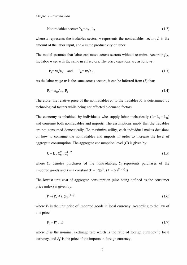
Nontradables sector: Yn= an. Ln (1.2)
where x represents the tradables sector, n represents the nontradables sector, L is the
amount of the labor input, and a is the productivity of labor.
The model assumes that labor can move across sectors without restraint. Accordingly,
the labor wage w is the same in all sectors. The price equations are as follows:
Px= w/ax and Pn= w/an (1.3)
As the labor wage 𝑤 is the same across sectors, it can be inferred from (3) that:
Pn= ax/an. Px (1.4)
Therefore, the relative price of the nontradables 𝑃𝑛 to the tradable𝑠 𝑃𝑥 is determined by
technological factors while being not affected b demand factors.
The economy is inhabited by individuals who supply labor inelastically (L= Lx + Ln)
and consume both nontradables and imports. The assumptions imply that the tradables
are not consumed domestically. To maximize utility, each individual makes decisions
on how to consume the nontradables and imports in order to increase the level of
aggregate consumption. The aggregate consumption level (C) is given by:
C = k . Cnγ . Ct
1−γ (1.5)
where 𝐶𝑛 denotes purchases of the nontradables, 𝐶𝑡 represents purchases of the
imported goods and k is a constant (k = 1/[𝛾𝛾. (1 − 𝛾)(1−𝛾)])
The lowest unit cost of aggregate consumption (also being defined as the consumer
price index) is given by:
P =(Pn)γ). (Pt)1−γ (1.6)
where 𝑃𝑡 is the unit price of imported goods in local currency. According to the law of
one price:
Pt = Pt∗ / E (1.7)
where E is the nominal exchange rate which is the ratio of foreign currency to local
currency, and 𝑃𝑡∗ is the price of the imports in foreign currency.

Chapter 1 - Introduction
7
In a foreign economy, there are three different sectors: nontradables, intermediate, and
final goods. Similarly, the nontradables sector produces goods for foreigners only. This
sector requires labor as the only one factor. The production function of the nontradables
sector is:
Yn∗= an
∗ . Ln∗ (1.8)
Intermediate goods are used in the production of the final goods. Similar to the
nontradables sector, the production function is represented by:
Yi∗= ai
∗ . Li∗ (1.9)
Because labor can move freely across foreign sectors, the foreign wage is equal across
sectors. Accordingly, the price of foreign intermediate goods is:
Pn∗= ai
∗ /an∗ . Pi
∗ (1.10)
The production of the final goods is dependent upon two inputs. One is the primary
commodities, which are tradables produced by the rest of the world, and among them is
the domestic economy. Another is intermediate goods produced in foreign economy.
The final good is also called the tradables, which are produced by gathering the foreign
intermediate input 𝑌𝑖∗ and the foreign primary commodity 𝑌𝑥
∗:
Yt∗= v. (Yi
∗)β. (Yx∗)1−β (1.11)
Accordingly, the unit cost of a tradable good in foreign currency is given by:
Pt∗= (Pi
∗)β. (Px∗)1−β (1.12)
Foreign consumers are supposed to consume the foreign nontradables and the final
goods. Moreover, they supply labor to the different sectors at the same wage rate.
Therefore, the consumer price index for the foreign economy is given by:
P∗= (Pn∗)γ. (Pt
∗)1−γ (1.13)
The real exchange rate is understood as “the foreign price of the domestic basket of
consumption (EP) relative to the foreign price of the foreign basket of consumption
(P*)”, Cashin, Céspedes and Sahay (2004).

Chapter 1 - Introduction
8
From (4), (6), (10), and (13), the real exchange rate in the domestic economy is
determined by:
EP/P∗ = (ax
ai∗
an∗
a𝑛
Px∗
Pi∗)
γ
(1.14)
It can be inferred from the model that an increase in the international price of the
tradables (primary commodities) will make wages in the commodity sector increase.
Because wages across sectors are the same, the increase in wages will raise the relative
price of the nontradables and, thus, appreciate the real exchange rate.
1.5 Thesis structure
The thesis is divided into seven chapters as follows:
Chapter 1 (Introduction) provides an overview of the thesis including
background and motivation, objectives, research questions, contributions, and
underlying theory of the study.
Chapter 2 (Economic background) explains the reasons for choosing OECD and
ASEAN as the representatives for developed and developing countries. In
addition, this chapter also provides insight into the economic background of
OECD and ASEAN commodity-exporting countries.
Chapter 3 (Literature review) conducts a review of literature on the link between
exchange rate and commodity prices in OECD and ASEAN commodity-
exporting countries and other developed and developing countries.
Chapter 4 (Research methodology) introduces the research methods and data
collection procedures used in empirical analysis with the purpose of clarifying
the relationship between real effective exchange rate and real commodity prices
in the OECD and ASEAN commodity-exporting countries.
Chapter 5 (Results and discussion) analyses and discusses test results.
Chapter 6 (Policy implications) makes predictions for the relationship in
ASEAN commodity-exporting countries when they achieve “developed
country” status and provides suggestions for policy makers of ASEAN
commodity-exporting countries during the transition period.

Chapter 1 - Introduction
9
Chapter 7 (Conclusion) concludes the work presented in this thesis and
discusses limitations of the research as well as suggests future research
directions.
1.6 Summary
This introductory chapter provides an overview of thesis. It elucidates the background
and motivation for carrying out this study. The four main objectives of this thesis
include exploring the relationship between real exchange rate and real commodity
prices in OECD and ASEAN commodity-exporting countries, comparing the
relationship between the two groups of countries, clarifying factors causing the
differences in the relationship (if there are differences in the relationship between the
two groups of countries) and giving guidelines for policy makers in ASEAN
commodity-exporting countries in their transition to become developed ones. A thesis
structure concludes the chapter. In the next chapter, the economic background of OECD
and ASEAN commodity-exporting countries is presented.

Chapter 2 – Economic background
10
Economic background
In this chapter, we explain the reasons for choosing OECD and ASEAN as the
representatives for developed and developing countries, respectively. In addition, some
basic information about OECD and ASEAN is given. However, not all countries within
these two groups are taken into account. As mentioned in Chapter 1, this thesis only
considers commodity-exporting countries when exploring the nexus between exchange
rate and commodity prices. This chapter also provides insight into the economic
backgrounds of six individual developed commodity-exporting countries in OECD –
Australia, Canada, Iceland, New Zealand, Norway and Greece – and six individual
developing commodity-exporting countries in ASEAN including Brunei, Laos,
Malaysia, Myanmar, Thailand, and Vietnam.
2.1 The OECD
The Organization for Economic Cooperation and Development (OECD) is an economic
organization established in 1961 (Wikipedia 2014b). The aims of OECD are “providing
a platform to compare policy experiences, seeking answers to common problems,
identifying good practices” that will improve the economic and social well being of its
member (Wikipedia 2014b). Until now, OECD has 34 members,2 most of which (31/34)
2 The 34 OECD member countries are: “Australia, Austria, Belgium, Canada, Chile, Czech Republic, Denmark, Estonia, Finland, France, Germany, Greece, Hungary, Iceland, Ireland, Israel, Italy, Japan, Korea, Luxembourg, Mexico, the Netherlands, New Zealand, Norway, Poland, Portugal, Slovak Republic, Slovenia, Spain, Sweden, Switzerland, Turkey, the United Kingdom, and the United States” (OECD).

Chapter 2 – Economic background
11
are developed economies with a very high Human Development Index. As can be seen
from the Figure 2.1, the material living standards (being measured by GDP per capita)
of OECD countries are much higher compared to that of other economies over the
period 2000 – 2012. Four countries having GDP per capita considerably in excess of
USD 40,000 in 2012 are Luxembourg, Norway, the United States and Switzerland
(OECD 2015). There are nine OECD countries having GDP per capita just above USD
40,000 and 12 countries having per capita GDP below USD 30, 000 in 20123 (OECD
2015).
Figure 2.1 – GDP per capita of OECD, ASEAN and others, 2000−2012
Source: Based on data from OECD Statistics and ASEAN Statistical Yearbook
However, the GDP growth rate of OECD countries in recent years is much lower than
that of the non-OECD countries. The average GDP growth rate of OECD in the period
2000 – 2012 is 1.67% while the rate of non-OECD countries is up to 6.48%.4 Being
affected severely by the recent financial crisis, the annual GDP growth rate for the
OECD area fell by 3.5% in 2009, which is the largest decrease on record. The economy
of OECD has recovered gradually after the crisis.
3 Countries that had GDP per capita just above USD 40,000 in 2012: Australia, Austria, Ireland, Sweden, Netherlands, Denmark, Canada, Germany, and Belgium. Countries that had GDP per capita below USD 30, 000 in 2012: Israel, Slovenia, Czech Republic, Slovak Republic, Greece, Portugal, Estonia, Chile, Poland, Hungary, Mexico, and Turkey (Source: OECD Statistics).
4 Source: OECD Statistics
0
5,000
10,000
15,000
20,000
25,000
30,000
35,000
40,000
OECD
China
India
South Africa
ASEAN
(USD
, cur
rent
pric
esan
d PP
Ps)

Chapter 2 – Economic background
12
Since its establishment, OECD has considered international trade as an efficient way of
raising living standards and boosting economic growth (OECD 2010). With the
progressive reduction of trade barriers, international trade in goods expanded
dramatically during the period between 2000 and 2008 in most OECD countries. In
2008/2009 the financial crisis resulted in the first huge decline (nearly one fourth) in
OECD merchandise trade (see Figure 2.2).
Figure 2.2 – International trade in goods of OECD and ASEAN 2000−2012
Source: Based on data from OECD Statistics and ASEAN Statistical Yearbook
Intra-OECD trade contributes a significant share of the total trade value (more than
70%) over the period. Nevertheless, there has been a gradual decline in this share from
76% in 2000 to 65% in 2012. Regarding non-OECD countries, the Asian area is the
largest trading partner of OECD. The trade with this area has risen from 8.3% of the
total OECD merchandise trade in 2000 to 14.5% in 20125. The main trade partners of
OECD countries are Germany, Japan, USA, UK, Europe and China.
As can be seen from Figure 2.3, OECD is not significantly dependent on commodity
export. During the last decade, in average, commodity export contributes about 19.1%
of total export.
5 All the data relevant to economic growth and trade are sourced from OECD Statistics.
0
5,000
10,000
15,000
20,000
25,000
OECD: imports
OECD: exports
ASEAN: imports
ASEAN: exports
OECD: total trade
ASEAN: total trade
(Bill
ion
USD
)

Chapter 2 – Economic background
13
Figure 2.3 – Commodity export and total export of OECD 1995−2013
Source: Based on data from UNCTAD
Table 2.1 – Top 15 export commodities in OECD 2007−2012
No. Commodities Average share of
Total OECD export
No. Commodities Average share of Total OECD
export 1 Crude oil 2.107% 9 Platinum 0.187% 2 Aluminum 1.201% 10 Corn 0.174% 3 Fish 0.605% 11 Soybeans 0.171% 4 Coal 0.595% 12 Coffee 0.126% 5 Iron 0.485% 13 Polypropylene 0.116% 6 Wheat 0.307% 14 Rice 0.098% 7 Swine meat 0.260% 15 Rubber 0.094% 8 Copper 0.247%
Source: Based on data from United Nations COMTRADE
The most significant commodity for the OECD is crude oil, which accounts for 2.1% of
total export value. Norway, Mexico and the United Kingdom are the three main
exporters of this commodity. Among non-oil commodities, metals are one of the most
prominent exports. The top five metals exported includes aluminium, iron, copper and
platinum. Cereals such as wheat, corn, soybeans and rice are also major exports of this
area. Fish ranks in the top three and most of the exports come from Norway, the United
States of America, Canada, and the Netherlands.
In respect to exchange rate, before 2006, soft pegs were the least persistent while hard
pegs are an absorbing state in the OECD. However after that, hard pegs shrank
considerably from approximately 35% in 2006 to 3% in 2007 as most European
countries changed from hard pegs to floating regimes (see Figure 2.4). From 2007 until
0100000020000003000000400000050000006000000700000080000009000000
10000000
1995
1996
1997
1998
1999
2000
2001
2002
2003
2004
2005
2006
2007
2008
2009
2010
2011
2012
2013
Mill
ions
of U
S do
llar
Total export
Commodityexport

Chapter 2 – Economic background
14
now, over 90% of OECD countries have operated flexible exchange rate regimes
because of their great benefit in terms of growth performance.
Figure 2.4 – Exchange rate arrangements in OECD 2003−2013
Source: Based on data from Annual Report on Exchange Arrangements and Exchange Restrictions
Note: (1) Hard pegs consisting of (a) exchange arrangements with no separate legal tender and (b) currency board
arrangements; (2) Soft pegs consisting of (a) conventional pegged arrangements, (b) pegged exchange rate within
horizontal bands, (c) crawling pegs, (d) stabilized arrangements and (e) crawl-like arrangements; (3) Floating regimes
comprising (a) managed floating and free-floating
2.2 The ASEAN
The Association of Southeast Asian Nations (ASEAN) was founded in 1967. This
organization aims to “accelerate economic growth, promote regional peace and stability,
and enhance cooperation on economic, social, cultural, technical, and educational
matters of Southeast Asian countries” (ASEANSecretariat 2014). Currently, ASEAN
has a total ten members6. However, these countries differ from each other in level of
development. Burma, Cambodia, Laos, and Vietnam, which are the last four countries
to join ASEAN, are much less developed than the other six member countries
(ASEANSecretariat 2014). Most ASEAN countries are developing economies, except
for Singapore and Brunei Darussalam. In 2012, the average GDP per capita of ASEAN
is USD 3,748, which is only one tenth of OECD’s (as illustrated in Figure 2.1).
6 The ten ASEAN member countries are: “Brunei Darussalam, Cambodia, Indonesia, Laos, Malaysia, Myanmar, Philippines, Singapore, Thailand, and Vietnam” (ASEANSecretariat 2014).
0%10%20%30%40%50%60%70%80%90%
100%
2003 2004 2005 2006 2007 2008 2009 2010 2011 2012 2013
Hard pegs Soft pegs Floating regimes Others

Chapter 2 – Economic background
15
The average GDP growth rate of ASEAN in the period 2000 – 2012 is 5.47%, which is
nearly three times higher than that of OECD. Being supported by a variety of
instruments related to trade in goods,7 both intra-ASEAN and extra-ASEAN trade has
been developing rapidly. Although the global financial crisis led to a dramatic decline in
ASEAN trade growth (from 17.78% in 2008 to −18.99% in 20098), the average annual
growth rate for the period 2000 – 2012 is still over 12%.9 In contrast with OECD
countries, intra-ASEAN trade only accounts for 25% while extra-ASEAN trade makes
up 75%; this proportion has remained relatively stable for the last decade. Among non-
ASEAN trading partners, China has contributed the greatest share since 2010. China –
ASEAN bilateral trade climbed rapidly at the average rate of 23.6% per year from 2002
to 2012. The other important trading partners of ASEAN are Europe, Japan, USA, and
Korean.
Figure 2.5 – Commodity export and total export of ASEAN 1995−2013
Source: Based on data from UNCTAD
ASEAN countries have vast mineral resources including both precious metals and
industrial ores (ASEAN 2014b). Similar to OECD, ASEAN is not overly reliant on
7 ASEAN has various instruments related to trade in goods: “(i) ASEAN Free Trade Area (AFTA, 1992), (ii) the ASEAN Agreement on Customs (1997), (iii) the ASEAN Framework Agreement on Mutual Recognition Arrangements (1998), (iv) the e-ASEAN Framework Agreement (2000); (v) the ASEAN Framework Agreement for the Integration of Priority Sectors (2004); (vi) the Agreement to Establish and Implement the ASEAN Single Windows (2005) and (vii) ASEAN–China Free Trade Area (2010)” (Secretariat 2011).
8 Source: ASEAN Merchandise Trade Statistics 9 Based on ASEAN Finance and Macroeconomics Surveillance Unit Database
0
200000
400000
600000
800000
1000000
1200000
1400000
1995
1996
1997
1998
1999
2000
2001
2002
2003
2004
2005
2006
2007
2008
2009
2010
2011
2012
2013
Mill
ions
of U
S do
llar
Total export
Commodityexport

Chapter 2 – Economic background
16
commodity export (except for Brunei). Commodity export accounts for approximately
28.5% of total export for the last decade (for more information, see Figure 2.5). In
respect to export commodities, crude oil is still the most important export for the
ASEAN area in the period from 2007 – 2012. The second largest commodity is rubber.
Fish and shrimp are two kinds of seafood that bring a great export value for the
ASEAN. Like OECD nations, such metals as aluminium, iron, copper, and platinum are
also on the top lists of exports (see Table 2.2).
Table 2.2 – Top 15 export commodities in ASEAN 2007−2012
No. Commodities Average share
of Total ASEAN export
No. Commodities Average share
of Total ASEAN export
1 Crude oil 2.370% 9 Pepper 0.064% 2 Rubber 1.845% 10 Nickel 0.048% 3 Fish 1.585% 11 Iron 0.038% 4 Palm oil 0.882% 12 Tobacco 0.040% 5 Rice 0.711% 13 Aluminum 0.027% 6 Shrimp 0.326% 14 Corn 0.018% 7 Copper 0.208% 15 Platinum 0.015% 8 Polypropylene 0.130%
Source: Based on data from United Nations COMTRADE
Figure 2.6 – Exchange rate arrangements in ASEAN 2003−2013
Source: Based on data from Annual Report on Exchange Arrangements and Exchange Restrictions
Note: (1) Hard pegs comprising (a) exchange arrangements with no separate legal tender and (b) currency board
arrangements; (2) Soft pegs comprising (a) conventional pegged arrangements, (b) pegged exchange rate within
horizontal bands, (c) crawling pegs, (d) stabilized arrangements and (e) crawl-like arrangements; (3) Floating regimes
comprising (a) managed floating and free-floating
0%10%20%30%40%50%60%70%80%90%
100%
2003 2004 2005 2006 2007 2008 2009 2010 2011 2012 2013
Hard pegs Soft pegs Floating Others

Chapter 2 – Economic background
17
In contrast to OECD, there is a relatively small number of ASEAN countries freely
floating their exchange rate (see Figure 2.6). Hard pegs are not preferred by ASEAN
countries. Brunei Darussalam is the only country operating this exchange rate
arrangement (currency board arrangements). Most ASEAN countries have adopted soft
pegs or else managed floating exchange rate regimes. However, since 2009, soft pegs
(mainly crawling pegs and stabilized arrangements) have become more popular than
managed floating regimes. Most of the ASEAN countries have witnessed many changes
in their exchange rate regimes over the last decade.
2.3 Why pick up OECD and ASEAN
It is well known that OECD is the largest group of developed countries in the world.
This organization comprises the 31 most advanced countries out of 49 developed
countries over the world. Therefore, OECD can be regarded as a good representative for
developed countries.
Regarding developing countries, there are four main areas of developing countries in the
world, which are ASEAN, Latin America,10 the South Asian Association for Regional
Cooperation (SAARC),11 and Sub-Saharan Africa.12 Among these groups of developing
countries, ASEAN becomes the focus of this thesis because it is the most similar to
OECD in terms of demographics, commodities export, financial markets, economic
performance, and development prospects. The similarity between the two groups of
developed and developing countries will be ideal for our purpose – giving helpful
10 Latin America is a region of America that comprises countries speaking Romance languages. They are “Argentina, Bolivia, Brazil, Chile, Colombia, Costa Rica, Cuba, Dominican Republic, Ecuador, El Salvador, French Guiana, Guatemala, Guadeloupe, Haiti, Honduras, Martinique, Mexico, Nicaragua, Panama, Peru, Puerto Rico, Saint Martin, Saint Barthelme, Uruguay and Venezuela” (Wikipedia).
11 SAARC comprises of eight members “Afghanistan, Bangladesh, Bhutan, India, Maldives, Nepal, Pakistan, and Sri Lanka” (Wikipedia).
12 Sub-Saharan Africa is the area of the continent of Africa, in the south of the Sahara Desert. Sub-Saharan Africa consists of 48 countries. They are “Angola, Benin, Botswana, Burkina Faso, Burundi, Cameroon, Cape Verde, Central African Republic, Chad, Comoros, Congo (Brazzaville), Congo (DRC-Kinshasa), Cote d’Ivoire, Djibouti, Equatorial Guinea, Eritrea, Ethiopia, Gabon, Gambia, Ghana, Guinea, Guinea-Bissau, Kenya, Lesotho, Liberia, Madagascar, Malawi, Mali, Mauritania, Mauritius, Mozambique, Niger, Nigeria, Reunion, Rwanda, Sao Tome and Principle, Senegal, Seychelles, Sierra Leone, Somalia, South Africa, Sudan, Swaziland, Tanzania, Togo, Uganda, Zambia, and Zimbabwe” (Countriesandcities 2015).
Chapter 2 – Economic background
18
guidelines for commodity-exporting developing countries in the management of
commodity prices and exchange rate in their transition period into developed countries.
With respect to population, SAARC is the most densely populated region among the
four developing groups with a population density of 31813 people per square kilometer
(2012), while the population density of ASEAN, Latin America, and Sub-Saharan
Africa are 132, 14 30, and 36 15 respectively. SAARC is by far more populous than
OECD, in which the population density in 2012 is merely 37 16 people per square
kilometer.
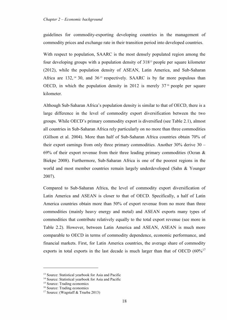
Although Sub-Saharan Africa’s population density is similar to that of OECD, there is a
large difference in the level of commodity export diversification between the two
groups. While OECD’s primary commodity export is diversified (see Table 2.1), almost
all countries in Sub-Saharan Africa rely particularly on no more than three commodities
(Gillson et al. 2004). More than half of Sub-Saharan Africa countries obtain 70% of
their export earnings from only three primary commodities. Another 30% derive 30 –
69% of their export revenue from their three leading primary commodities (Ocran &
Biekpe 2008). Furthermore, Sub-Saharan Africa is one of the poorest regions in the
world and most member countries remain largely underdeveloped (Sahn & Younger
2007).
Compared to Sub-Saharan Africa, the level of commodity export diversification of
Latin America and ASEAN is closer to that of OECD. Specifically, a half of Latin
America countries obtain more than 50% of export revenue from no more than three
commodities (mainly heavy energy and metal) and ASEAN exports many types of
commodities that contribute relatively equally to the total export revenue (see more in
Table 2.2). However, between Latin America and ASEAN, ASEAN is much more
comparable to OECD in terms of commodity dependence, economic performance, and
financial markets. First, for Latin America countries, the average share of commodity
exports in total exports in the last decade is much larger than that of OECD (60%17
13 Source: Statistical yearbook for Asia and Pacific 14 Source: Statistical yearbook for Asia and Pacific 15 Source: Trading economics 16 Source: Trading economics 17 Source: (Wagstaff & Trueba 2013)

Chapter 2 – Economic background
19
compared to 19.1%18) while the average share of ASEAN is 28.5%,19 which is much
closer to that of OECD. Second, the economic performance of ASEAN is much better
than that of Latin America for the last three decades (Zermeño, Preciado & Vásquez
2011). Specifically, ASEAN had longer periods of macroeconomic stability. The
average real growth rate, investment and the exports growth (as a proportion in GDP) in
ASEAN are considerably larger than those of Latin America. Lastly, the financial
market of ASEAN is much more advanced with substantially higher bank credit to the
private sector, liquidity, and stock market capitalization over GDP. In addition,
Zermeño, Preciado and Vásquez (2011) show that while the growth of the stock market
has had a positive effect in ASEAN, it has had adverse effects in Latin America. Latin
America countries now are faced with systematic weaknesses in many of the structural
foundations that are needed for growth and are confronted with growing poverty,
deindustrialization, and social polarization. It is likely to take a long time for Latin
America to solve current problems (Hillebrand 2003).
Moreover, OECD and ASEAN have the same main trade partners, which are China,
Europe, Japan, USA and UK. And, both groups have similar main export commodities
consisting of crude oil, aluminium, fish, iron, copper, platinum, rice and rubber (for
more information see Table 2.1 and Table 2.2).
It is also worth mentioning that ASEAN countries build development prospects that are
parallel to current OECD. As mentioned in Section 6.1, ASEAN countries aim to
become an ASEAN integrated economic region. This development plan involves
developing the financial market, expanding the service industry (for emerging market
countries) or boosting industrialization (for CLMV countries20) while shrinking the
dependence on the agriculture sector and natural resources, boosting investment and
free trade in the region, and developing human resources, technology, and science.
From the above discussion, ASEAN is the most comparable to OECD, with respect to
demographics, commodities export, financial markets, economic performance, and
development prospects. Based on the similarity between OECD and ASEAN, this thesis
18 Source: Being calculated based on UNCTAD 19 Source: Being calculated based on UNCTAD 20 CLMV countries are Cambodia, Laos, Myanmar and Vietnam

Chapter 2 – Economic background
20
is expected to provide significant policy implications for ASEAN commodity-exporting
countries in management of exchange rates and commodity prices on their way to
achieving “developed country” status.
2.4 Commodity-exporting countries
This section provides insight into the economic backgrounds of individual OECD and
ASEAN commodity-exporting countries. Specifically, basic information about
economic structure, economic development in recent decades, trading, export
commodities as well as exchange rate is provided for each country.
2.4.1 OECD commodity-exporting countries
2.4.1.1 Australia
Australia is a developed country with a GDP per capita of USD 44,407 as of 2012.
Before the 1980s, Australia was a relatively closed and protectionist economy
(Economywatch 2015a). Since 1983, the Australian government has carried out such
key economic reforms as removing some non-tariff barriers, cutting high tariffs,
liberalizing the financial services sector, floating the Australian dollar, enhancing the
efficiency of the government system, privatizing government-owned industries, and
restructuring the tax system (Economywatch 2015a). Thank to these reforms, Australia
has turned into an open, export-oriented market economy (Economywatch 2015a).
The Australian economy has expanded gradually by an average rate of 3.12% during the
period 2000-2012 while maintaining low unemployment, low inflation, and very low
public debt (Indexmundi 2014a). Australia has experienced the longest period (21
years) of economic expansion without being affected by global recessions.
The service sector is regarded as the backbone of Australia’s economy, accounting for
68.8% of GDP in 2012 (Economywatch 2015a). Meanwhile, the agriculture sector only
makes a small contribution to GDP (4% in 2012) (Economywatch 2015a). In the last
decade, the mining industry has been the promoter for Australia’s economic
development (Economywatch 2015a). Australia is the largest producer of coal, lead,
rutile, zircon, nickel, tantalum, and uranium in the world (Economywatch 2015a).

Chapter 2 – Economic background
21
Figure 2.7 – GDP per capita of Australia, Canada, Iceland, New Zealand,
Norway, and Greece 2000−2013
Source: OECD Factbook 2014
During the period from 2000 to 2013, the Australia’s exports have increased rapidly
(nearly four fold) except for a slight decrease in 2008. This increase is explained by a
higher demand for Australia's commodities coming from the rapid urbanization and
industrialization of China and India (Atkin & Connolly 2013).
Being rich in natural resources, Australia is one of the largest exporters of commodities
in the world. Major export commodities are minerals such as iron, coal, gold, and
agricultural products such as wheat, cotton, beef and lamb, and energy in the forms of
petroleum gas and coal.
Table 2.3 – Top 20 export commodities in Australia 2000−2013
No. Commodities Average export value 2000-2013
(USD) No. Commodities
Average export value 2000-2013
(USD) 1 Iron 29,430,855,430 11 Diamond 1,533,009,770 2 Coal 23,473,211,210 12 Lamb 1,242,899,500 3 Gold 8,606,424,200 13 Cotton 1,196,165,800 4 Petroleum gas 6,644,116,410 14 Zinc 1,170,448,000 5 Crude oil 6,382,390,670 15 Natural gas 1,075,480,810 6 Titanium 4,467,229,700 16 Barley 878,390,480 7 Beef 3,906,558,000 17 Nickel 755,629,320 8 Wheat 3,699,147,020 18 Lead 721,987,850 9 Copper 3,230,834,600 19 Shrimp 459,644,590
10 Oil petroleum 2,244,499,874 20 Uranium 306,603,430
Source: Based on data from United Nations COMTRADE
0
10000
20000
30000
40000
50000
60000
70000U
SD, c
urre
nt p
rice
s and
PPP
s
Australia
Canada
Greece
Iceland
New Zealand
Norway

Chapter 2 – Economic background
22
The largest export markets of Australia are Japan, China, South Korea, India and the
United States (Tradingeconomics 2015a). In recent years, Australia's trade has shifted
from traditional destinations such as the United States and Europe toward emerging
Asian countries. Beginning in 2009, China has become Australia's largest export
destination (Embassy 2011) and in 2014, China accounted for 31.9% of Australia's
exports (Tradingeconomics 2015a).
In regard to the exchange rate regime, the development history of the exchange rate
regime of Australia has gone through three stages: fixed, then managed floating, and
finally the independently floating (Internationaleconomics 2015). Specifically, in the
Bretton Woods period (from 1945 to 1973), Australia followed fixed exchange rates.
After the breakdown of the Bretton Woods system (1973), Australia began to adopt a
managed floating system. In this system, the exchange level was set daily by the
Reserve Bank based on a trade-weighted currency basket (Internationaleconomics
2015). Until 1983, Australia decided to float the exchange rate for a few reasons.
Firstly, the fixed exchange rate regime impeded the control of the money supply.
Secondly, at that time, Australia pursued a “monetary targeting” policy with the aim of
increasing the money supply (RBA 2015). Nevertheless, under the fixed and crawling
peg arrangements, the Reserve Bank has a duty to meet all requests to exchange foreign
currency for Australian dollars and vice versa (RBA 2015). This implied that the supply
of Australian dollars was affected by fluctuations in the purchases and sales demand of
Australian dollars, which could arise from Australia's international trade and capital
flows (RBA 2015). It was difficult for the Reserve Bank of Australia to offset these
effects through sterilization. Floating the exchange rate was regarded as a proper
solution for this problem (RBA 2015).
2.4.1.2 Canada
Canada is one of the most advanced nations in the world. The growth of Canada’s
economy is linked with the economy of the United States (Wikipedia 2014a). After the
United States – Canada Free Trade Agreement (FTA) and the North American Free
Trade Agreement (NAFTA) were signed (in 1989 and 1994, respectively), trading and
economic integration between the two countries has increased dramatically. From 1993
to 2007, Canada had strong economic growth. After being affected significantly by the
global economic crisis of in 2008 – 2009, Canada suffered the first fiscal deficit in 2009

Chapter 2 – Economic background
23
after a long time of surplus (CIA 2012). However, Canada recovered from the crisis
quite quickly owing to appropriate monetary and fiscal stimulus, a robust financial
system and high commodity prices (OECD 2012). Canada has attained marginal growth
since 2010 and expects to balance the budget by 2015 (CIA 2012).
In 2012, Canada’s GDP composition was as follows: services (66.1%), industry (32%)
and agriculture (1.9%). Although the contribution of agriculture to GDP is limited,
Canada is one of the largest suppliers of agricultural products in the world
(Economywatch 2015b).
Table 2.4 – Top 20 export commodities in Canada 2000−2013
No. Commodities Average export value 2000-2013
(USD) No. Commodities
Average export value 2000-2013
(USD) 1 Crude oil 46,021,519,390 11 Shrimp 1,637,196,020 2 Petroleum gas 21,818,947,410 12 Beef 1,019,047,680 3 Oil petroleum 13,023,524,970 13 Soybeans 966,707,340 4 Gold 8,603,450,460 14 Fish 882,731,190 5 Wheat 4,490,557,470 15 Barley 358,391,540 6 Coal 4,211,238,740 16 Oats 331,052,450 7 Iron 2,551,291,670 17 Coffee 305,579,870 8 Swine meat 2,029,743,930 18 Zinc 256,329,580 9 Diamond 2,003,987,270 19 Maize 253,255,270 10 Copper 1,703,806,520 20 Tobacco 176,440,130
Source: Based on data from United Nations COMTRADE
In the past, fishing and forestry were the major industries in Canada (Economywatch
2015b). Although these two industries maintain the important roles in Canada’s
economy currently, mineral and energy resources have turned into the main source of
income for this country (Economywatch 2015b). Canada is the leading mineral exporter
in the world with such commodities as gold, iron, nickel, zinc, and copper
(Economywatch 2015b). Besides, unlike most developed countries, this country is a net
exporter of energy (mainly coal, oil, natural gas). Canada is also among the world’s top
ten largest oil exporters and top three largest natural gas exporters (Economywatch
2015b).
The main trading partners of this country are the United States, China, and the United
Kingdom which account for 74.5%, 4.3% and 4.1% of Canada’s total trade in 2012,
respectively (OECD 2012). Although Canada has increased energy product exports to

Chapter 2 – Economic background
24
China dramatically in recent years, the United States is still by far its largest trading
partner.
Regarding the exchange rate, Canada is the developed nation that has experienced the
longest duration with a floating exchange rate. In 1950, Canada became the first
developed nation to float its exchange rate (Thiessen 2000). By floating the exchange
rate, the Canadian currency appreciated dramatically. This appreciation discouraged
further capital inflows and maintained Canada’s monetary policy autonomy (Thiessen
2000). In 1962, Canadian currency turned back to a fixed exchange rate and pegged it
tightly to the USD. This regime had been remained for eight years (Thiessen 2000). In
1970, Canada was the first Western country to move to a free-floating exchange rate
again. From that time until now, Canada has continued following a free-floating
exchange rate regime (Thiessen 2000). This regime allows Canada to have monetary
conditions that are different from the United States and more appropriate to Canada’s
own economic situations (Thiessen 2000). Another advantage of this exchange rate
regime is that it enables Canada to respond properly to external economic shocks
affecting Canada differently from the United States (Thiessen 2000).
2.4.1.3 Iceland
Iceland is an advanced country located in the North Atlantic (Wikipedia 2014b).
Although Iceland’s economy is the smallest within the OECD, the GDP per capita of
this country is among the highest at about USD 39,097 in 2012. In 2007, Iceland ranks
1st in Human Development Index in the world.
In the past, fishing and agriculture were the major sectors in Iceland (Wikipedia 2014b).
In recent years, there has been a dramatic change in economic structure with a large
expansion of manufacturing and service industries, particularly within the fields of
software production, biotechnology, and tourism (CIA 2014b). These two sectors have
exceeded the fishing and agriculture sectors, both in terms of labor and contribution to
GDP. In particular, Iceland has experienced tenfold increase in the number of foreign
visitors within the last four decades. Besides, there is rapid growth in the software
industry; in the last ten years, it has grown by over 50% annually and software exports
now account for 5% of Icelandic service exports.

Chapter 2 – Economic background
25
Prior to the global financial crisis, Iceland achieved a high economic growth rate (the
average rate for the period 2000 – 2008 was 4.18%) and low unemployment. In October
2008, the collapse of Iceland’s three major banks brought dramatic changes for
Iceland’s economy (ICoC 2012). As a consequence of the banking crisis, Iceland
entered a deep recession. Specifically, in 2009, GDP declined 6.8% while the
unemployment rate was as high as 9.4% (CIA 2014b). The Icelandic government
implemented some measures to overcome these difficulties including “stabilizing the
Krona, implementing capital controls, reducing Iceland’s high budget deficit, containing
inflation, addressing high household debt, restructuring the financial sector and
diversifying the economy” (Indexmundi 2014c). Owing to appropriate reforms, the
Icelandic economy has been recovered since late 2010, and achieved an economic
growth rate of 1.4% in 2012.21
Iceland's economy is highly export-driven. Although the role of the fishing industry in
Iceland’s economy has declined, the fishing industry is still one of the foundations of
the Icelandic economy with approximately 70% of its export earnings obtained through
fish, shrimp, and fish-related products. Iceland is one of the largest exporters of fish and
fishery products to the EU (EuropeanCommission 2015). Besides, Iceland also exports
such agricultural commodities as coffee, bananas, beef, cotton, rubber, and orange juice.
However, the export value of these commodities is not considerable.
Table 2.5 – Top 20 export commodities in Iceland 2000−2013
No. Commodities
Average export value 2000-2013
(USD)
No. Commodities
Average export value 2000-2013
(USD) 1 Fish 425,980,100 11 Coffee 38,910 2 Fish meal 358,524,170 12 Bananas 13,140 3 Oil petroleum 45,341,560 13 Beef 11,450 4 Shrimp 42,032,800 14 Cotton 7,660 5 Lamb 10,993,380 15 Rubber 6,410 6 Rice 8,824,350 16 Orange juice 5,920 7 Fish 4,764,590 17 Pearl 5,280 8 Swine meat 58,360 18 Coconut 2,520 9 Gold 44,870 19 Maize 2,200 10 Natural gas 39,600 20 Zinc 2,120
Source: Based on data from United Nations COMTRADE
21 Source: OECD Statistics

Chapter 2 – Economic background
26
Iceland entered into a free trade agreement covering all industrial products with the EU
in 1972 and ratified the European Economic Area Agreement (EEA) in the 1990s.
These treaties have strengthened foreign trade with the EU. This area is the largest
market area for Iceland’s commodities exports. However, there was a slight decline in
the share of exports to this area in the last five years. In 2008, exports to the EU
accounts for 80.5% of the total exports, then this share decreased to 78.3% in 2012
(Iceland 2013b). The Netherlands is the greatest export partner of Iceland, contributing
24% of Iceland’s total exports (Iceland 2013b). Other major export partners of Iceland
are Germany, Spain, Ireland, and the United Kingdom.
Iceland adopted a floating exchange rate rather late (in 2001) compared to other OECD
countries. After the Bretton Woods fixed rate system collapsed in 1974, Iceland started
following a managed floating exchange rate. This exchange rate regime has been
continued until 1983. However, in the mid-1980s, the country employed a more
restrictive monetary and exchange rate policy (Gudmundsson 2000). This made the
Icelandic Krona devalue dramatically. After this period, Icelandic monetary authorities
kept the Krona value stable against the USD and different baskets of trading partner’s
currencies (Gudmundsson 2002). In 1900, the Central Bank of Iceland emphasized on
price stability (ICoC 2012). As the result, exchange rates had to play the role of a
monetary anchor, instead of an adjustment instrument (Gudmundsson 2002). Since
2001, Iceland has floated its exchange rate.
2.4.1.4 New Zealand
New Zealand is a Pacific nation with a relatively high living standard. The GDP per
capita of this country in 2012 is USD 32,847 (Economywatch 2015f).
New Zealand is a diversified economy with a wide range of sectors. The agricultural
system of New Zealand is well known for its efficiency. Agricultural products are the
main exports of New Zealand. However, the agriculture sector makes a humble
contribution to GDP (Economywatch 2015f). Like other advanced economies, the
service sector is the backbone of New Zealand’s economy. In 2009, the GDP
composition of New Zealand was as follows – services (nearly 70%), industry (nearly
26%) and agriculture (about 4%). The main industrial sectors consist of food
processing, textiles, machinery, mining and transportation equipment (Economywatch

Chapter 2 – Economic background
27
2015f). Generally, all sectors of the economy have shown growth in recent decades.
Among them, petroleum and minerals are the two sectors that have enjoyed the most
rapid growth. During the period 2000 – 2012, New Zealand’s economy expanded
considerably at an average annual economic growth rate of 2.92%.
New Zealand’s economy had been negatively influenced by the global financial crisis
for five uninterrupted quarters in 2008 – 2009 (IBP 2013a). By implementing such
measures as cutting interest rates aggressively and developing fiscal stimulus measures,
New Zealand recovered its economy in late 2009 (Indexmundi 2014d). The economy
continuously achieved approximately 2 – 3% per year growth in the period 2010 –
2013. However, key trade sectors are still lagging behind because of weak external
demand (IBP 2013a).
New Zealand is an export-oriented economy (Tradingeconomics 2015b). Most of the
exports are primary commodities (75% of total exports in 2012). Among primary
commodities, dairy products such as milk powder, butter, and cheese are the leading
export commodities for which export value accounts for 25% of the total export
(Bancorp 2013). Apart from dairy products, other major agricultural export
commodities include lamb, beef, fish, fishmeal, cotton, maize, coffee, tea and barley.
Furthermore, oil, gold, and iron are also important export commodities of New Zealand.
Table 2.6 – Top 20 export commodities in New Zealand 2000−2013
No. Commodities
Average export value 2000-2013
(USD)
No. Commodities
Average export value 2000-2013
(USD) 1 Dairy 4,212,446,600 11 Iron 24,634,740 2 Lamb 1,836,194,670 12 Petroleum gas 8,156,360 3 Beef 1,334,121,770 13 Fishmeal 6,239,110 4 Fish 252,066,380 14 Cotton 5,888,610 5 Crude oil 822,223,530 15 Maize 4,144,860 6 Gold 270,224,110 16 Coffee 2,066,630 7 Coal 247,538,770 17 Pearl 1,227,910 8 Shrimp 137,257,800 18 Platinum 978,000 9 Diamond 38,036,090 19 Tea 976,860 10 Tobacco 25,741,340 20 Barley 912,260
Source: Based on data from United Nations COMTRADE
New Zealand’s export partners are Australia, China, Japan, the United Kingdom, the
United States, Singapore, Hong Kong, India, and Germany (Tradingeconomics 2015b).

Chapter 2 – Economic background
28
For the last 40 years, New Zealand’s export markets have undergone a fundamental
transition from Northern hemisphere countries to the Asia-Pacific region, making the
share of export goods to the Asia-Pacific region increase from 20% in 1966 to 88% in
2011 (Indexmundi 2014d).
Although there has been an increase in trading with China in recent years, Australia is
still the most significant importer with the share of export goods to this country of
21.1% in 2012 (Indexmundi 2014d).
After the fall of Bretton Woods, the monetary authorities have used many exchange rate
regimes to pursue different objectives. To cope with a series of currency crises around
the world in the 1960s and early 1970s, New Zealand temporarily restabilised its
currency in 1971 (Sullivan 2013). Following Australia, the New Zealand dollar (NZD)
was originally pegged to the USD at its par value (Sullivan 2013). Because of this
arrangement, the NZD dramatically depreciated against other currencies. In 1973, this
country stopped pegging to the USD and started adopting a fixed exchange rate against
a basket of currencies with occasional discrete adjustment (Sullivan 2013).
The adjustment of the NZD is aimed at maintaining competitiveness with Australia.
Nonetheless, the changes in the nominal exchange rate unintentionally made the terms
of trade as well as inflation rates fluctuate in the 1970s. Moreover, the variations of the
nominal exchange rate were also an obstacle for exporters (Sullivan 2013). By 1979,
New Zealand recognized that it needed a more flexible system. Therefore, a crawling
peg was introduced. Under this system, small adjustments for the NZD were frequently
made based on relative inflation in order to main trading partners (Sullivan 2013). In
1982, when wage and price freeze was introduced, the Reserve Bank of New Zealand
abandoned a crawling peg regime and adopted a fixed exchange rate against its basket
(occasionally adjustable). As the NZD devaluates considerably in response to the
devaluation of AUD, New Zealand recognized that it is unsustainable to maintain the
level of the NZD (Sullivan 2013). Then, New Zealand freely floated its NZD in March
1985.

Chapter 2 – Economic background
29
2.4.1.5 Norway
Among European countries, Norway is a country with a very high standard of living and
a developed welfare system (Wikipedia 2015h). The GPD per capita of this nation in
2012 was USD 66,135, ranking second (only behind Luxembourg) in the OECD.
Norway enjoyed solid GDP growth in the period of fifteen years (more than 5%
annually in average) before a slowdown in 2008 and 2009. On the whole, Norway’s
economy was less impacted by the global crisis than other developed countries. This
resilience owes to the petroleum wealth and a sound macroeconomic policy framework.
After a negative growth in 2009 (−1.6%), the Norwegian economy has gained positive
growth since 2010 (Indexmundi 2014e).
Norway is rich in natural resources. The most valuable natural resources of this country
are crude oil and natural gas, hydropower, forests, fish, shrimp, and minerals. Crude oil
and natural gas represented the largest share of total exports in 2012 (70%). Norway is
the leading supplier of natural gas to Western Europe. Moreover, it is also the third
largest oil exporter in the world (Economywatch 2015g).
With a coastline of more than 83,000 km, the fishery industry plays an important role in
Norwegian society and economy. Seafood products are the second most important
export item in Norway. In 2012, seafood export value reached USD 8.9 billion, making
up 6% of total Norwegian goods exports. Moreover, Norway also ranks 1st in fish
exports in the world (Economywatch 2015g).
Apart from oil, natural gas and seafood products, minerals including gold, platinum,
iron, zinc, and nickel and agricultural products consisting of soybeans, cotton, tobacco,
coffee, beef, swine meat, and lamb are the main export commodities of this country
during the period 2000 – 2013.
High dependence on natural resources makes the economic growth of Norway
vulnerable to fluctuations in the external demand for these commodities as well as their
prices (Wikipedia 2015h). Recognizing the problems, since 1970s, the Norwegian
government has launched some policies to encourage the development of new
industries, especially a high-tech industry, in the private sector (Wikipedia 2015h). The
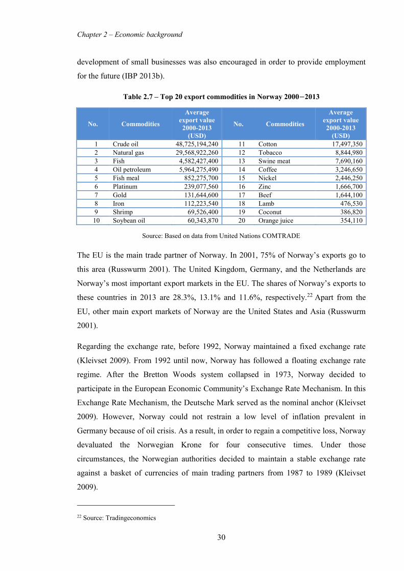
Chapter 2 – Economic background
30
development of small businesses was also encouraged in order to provide employment
for the future (IBP 2013b).
Table 2.7 – Top 20 export commodities in Norway 2000−2013
No. Commodities
Average export value 2000-2013
(USD)
No. Commodities
Average export value 2000-2013
(USD) 1 Crude oil 48,725,194,240 11 Cotton 17,497,350 2 Natural gas 29,568,922,260 12 Tobacco 8,844,980 3 Fish 4,582,427,400 13 Swine meat 7,690,160 4 Oil petroleum 5,964,275,490 14 Coffee 3,246,650 5 Fish meal 852,275,700 15 Nickel 2,446,250 6 Platinum 239,077,560 16 Zinc 1,666,700 7 Gold 131,644,600 17 Beef 1,644,100 8 Iron 112,223,540 18 Lamb 476,530 9 Shrimp 69,526,400 19 Coconut 386,820 10 Soybean oil 60,343,870 20 Orange juice 354,110
Source: Based on data from United Nations COMTRADE
The EU is the main trade partner of Norway. In 2001, 75% of Norway’s exports go to
this area (Russwurm 2001). The United Kingdom, Germany, and the Netherlands are
Norway’s most important export markets in the EU. The shares of Norway’s exports to
these countries in 2013 are 28.3%, 13.1% and 11.6%, respectively.22 Apart from the
EU, other main export markets of Norway are the United States and Asia (Russwurm
2001).
Regarding the exchange rate, before 1992, Norway maintained a fixed exchange rate
(Kleivset 2009). From 1992 until now, Norway has followed a floating exchange rate
regime. After the Bretton Woods system collapsed in 1973, Norway decided to
participate in the European Economic Community’s Exchange Rate Mechanism. In this
Exchange Rate Mechanism, the Deutsche Mark served as the nominal anchor (Kleivset
2009). However, Norway could not restrain a low level of inflation prevalent in
Germany because of oil crisis. As a result, in order to regain a competitive loss, Norway
devaluated the Norwegian Krone for four consecutive times. Under those
circumstances, the Norwegian authorities decided to maintain a stable exchange rate
against a basket of currencies of main trading partners from 1987 to 1989 (Kleivset
2009).
22 Source: Tradingeconomics

Chapter 2 – Economic background
31
In 1990, the reunification of Germany caused a rise in demand, which led to an increase
in interest rates. This interest rate increase had negative impact on participants of the
Exchange Rate Mechanism. As a result, Norway was compelled to allow their currency
to float in December 1992 (Kleivset 2009). Although going through some changes, the
Norway has still maintained a floating exchange rate regime until today.
2.4.1.6 Greece
Greece is a developed country in Southern Europe with a population of 10,993,000
people (Wikipedia 2015f). The Human Development Index of Greece ranks 29th in the
world.
Before 2008, Greece had a long period of economic growth. Because of the impact of
the Global economic crisis, Greece went into recession in 2008 (Wikipedia 2015f).
Since the restoration of democracy in 1974, this is the most severe crisis faced by the
Greek economy. In 2009, this country suffered the highest budget deficit and
government debt-to-GDP ratios in Europe (Wikipedia 2015f). Moreover, the garment
industry, a backbone of the Greek economy, has been the most vulnerable sector in the
recession. And, there was a large decline in the retail turnover in 2010 – 2011
(Secretariat 2013). In addition, unemployment rose steeply from 7.2% in 2008 to 27.9%
in 2013 (Secretariat 2009b; Secretariat 2013). It is worth noting that youth
unemployment in this country amounted to 64.9% in 2013. In 2014, Greece enjoyed its
first quarter of economic growth since 2008. Currently, this country can balance its
budget and re-entered financial markets.
The services sector is a significant part of Greece’s economy and represents about
80.6% of Greece’s GDP in 2014. The industry sector accounts for about 15.9% of this
country’s GDP (CIA 2014a).
Greece mainly exports food and beverages, petroleum products, textiles and chemicals
(Economywatch 2015c). The main trading partners are EU countries, the United States
and China. In terms of export volume, Greece ranked 65th in the world and far below the
EU rankings.

Chapter 2 – Economic background
32
Apart from manufactured products, Greece also exports primary commodities such as
olive oil, cotton, fish, dairy, crude oil, wheat, hides, and rice. Among them, olive oil and
cotton are the most significant export commodities of Greece (see Table 2.8).
Table 2.8 – Top 20 export commodities in Greece 2000 −2013
No. Commodities
Average export value 2000-2013
(USD)
No. Commodities
Average export value 2000-2013
(USD) 1 Olive oil 341,686,800 11 Coffee 9,633,300 2 Cotton 320,146,890 12 Soybean oil 9,548,770 3 Fish 215,390,510 13 Banana 8,018,480 4 Dairy 132,192,710 14 Zinc 6,932,130 5 Crude oil 61,772,400 15 Poultry 6,872,900 6 Wheat 54,050,600 16 Hard Sawn 6,865,410 7 Hides 45,495,460 17 Sugar 5,725,750 8 Rice 25,268,185 18 Sunflower oil 5,685,225 9 Aluminum 22,637,850 19 Beef 4,852,433 10 Corn 13,345,000 20 Wool 4,547,199
Source: Based on data from United Nations COMTRADE
Regarding imports, the main imported commodities are machinery, transport
equipment, fuels and chemicals. Import partners of this country are the EU, Russia, and
China.
The drachma had been the currency of Greece for the period from 1832 to 2001. For
every working day, the Bank of Greece had to organize a Fixing session in order to set
the official exchange rate of the drachma against foreign currencies. This session took
place under the control of the Bank of Greece as well as the participation of authorized
representatives of all authorities in foreign exchange transactions banks (Greece 2000).
Greece officially joined the Eurozone in 2001. At that time, Greece adopted the Euro at
the fixed exchange rate of 340.75 Drachma to 1 Euro (Wikipedia 2015f). However, only
until January 2002 there was a physical exchange from Drachma to Euro (Wikipedia
2015f).
At the time when Greece joined the Eurozone officially (2001), Greece decided to
abandon a managed floating exchange rate to in order to adopt a free-floating one.

Chapter 2 – Economic background
33
2.4.2 ASEAN commodity-exporting countries
2.4.2.1 Brunei
Brunei is a small but wealthy economy. With a population of 417,784, Brunei people
have a high-quality life with GDP per capita of USD 38,563 in 2013. The GDP per
capita of Brunei ranks 2nd in ASEAN, after only Singapore (Embassy). Different from
other countries in ASEAN, the economic growth of Brunei is slow and steady
(Embassy).
Brunei’s economy is totally dependent on the exports of crude oil (Wikipedia 2015b).
As can be seen from Table 2.9, during the period from 2000 – 2013, the export revenue
from crude oil is by far larger than other commodities. It is the third largest oil exporter
in ASEAN. On average, Brunei produces about 180,000 barrels per day (Wikipedia
2015b).
Figure 2.8 – GDP per capita of Brunei, Laos, Malaysia, Myanmar, Thailand, and
Vietnam 2000−2013
Source: ASEAN Statistic Yearbook
Apart from petroleum products, Brunei only produces some kinds of products locally
(IBP 2011). Most of main manufactured products and foods are imported from other
countries. Brunei imports around 80% of its total food requirements (DFAT 2013).
0
5000
10000
15000
20000
25000
30000
35000
40000
45000
USD
, cur
rent
pri
ces a
nd P
PPs
Brunei
Laos
Malaysia
Myanmar
Thailand
Vietnam

Chapter 2 – Economic background
34
Table 2.9 – Top 20 export commodities in Brunei 2000−2013
No. Commodities
Average export value 2000-2013
(USD)
No. Commodities
Average export value 2000-2013
(USD) 1 Crude oil 1,677,926,830 11 Coconut oil 6,030 2 Hides 282,040 12 Banana 5,410 3 Sunflower oil 151,250 13 Soybeans 4,480 4 Fish 105,710 14 Tea 1,560 5 Beef 94,310 15 Aluminum 890 6 Hard sawn 75,550 16 Hard log 770 7 Chicken 71,260 17 Coffee 700 8 Dairy 52,670 18 Corn 640 9 Shrimp 28,820 19 Sugar 475 10 pork 24,010 20 Natural gas 425
Source: Based on data from United Nations COMTRADE
Singapore is the largest import partner of Brunei. Brunei’s imports from Singapore
amounted to 20.5% of its total imports. Other import partners are China, Japan,
Malaysia and the United States (Wordsrichestcountries 2014). Main imported goods are
construction, electronic, medical and technical equipment, pharmaceuticals and
household appliances (Wordsrichestcountries 2014).
Although being highly reliant on energy products, this sector employs only 3% of
Brunei’s labor force. The public sector is the sector that provides most of the
employment for this country. More than half of the workforce is employed by this
sector (DFAT 2013).
Brunei has a long-term plan to reduce the over reliance on fossil fuels and diversify its
economy. To achieve this goal, this country will develop a private non-energy sector,
promote investment, increase food self-sufficiency and encourage the participation of
women in workforce (Cooke 2012).
The Brunei dollar has been the currency of Brunei since 1967. Brunei has adopted a
currency boards arrangement since independence. Brunei Darussalam ties its currency
to the Singapore dollar. Brunei adopted a currency board arrangement partly because of
their limited central banking expertise (IMF 1997). Moreover, the largest benefit of this
exchange rate regime is that the Brunei dollar is always backed by sufficient foreign
exchange reserves. The market and official exchange rates are equated owing to the
interchangeability arrangement between authorities of Brunei and Singapore. According

Chapter 2 – Economic background
35
to the interchangeability arrangement, banks of both countries accept and allow both
Brunei and Singapore dollars at parity (IMF 1997).
2.4.2.2 Laos
Laos is one of the poorest countries in ASEAN. The GDP of this country in 2013 is
11.24 billion USD (Wikipedia).
Since 1986, the economy of Laos has grown rapidly. This rapid development is
attributed to significant reforms in 1986, such as decentralizing control and encouraging
private enterprise (CIA 2014c). From 1988 to 2008, the average annual growth rate of
Laos was 6% and from 2008 to 2013 this rate increased to 7% (CIA 2014c).
Although the economy has grown rapidly in recent decades, Laos is still a poor country.
The main problems of Laos are a lack of infrastructure, corruption, and a largely
unskilled workforce (CIA 2014c). The government plans to solve these problems in the
future.
The economy of Laos still remains dependent on an unproductive agricultural sector.
This sector employs 75% of the workforce. In addition, such industries as handicrafts,
beer, coffee and tourism also play important roles in the economy (Wikipedia).
Laos’ economy is extremely reliant on international aid (CIA 2014c). Foreign direct
investment (FDI) is essential for large-scale infrastructure projects in Laos such as
Mekong river hydropower dams, copper and gold mining, logging, and construction
(CIA 2014c). Major sources of FDI are from China, Vietnam and Thailand. During the
period from 2001 to 2011, FDI from the three countries make up 78.26% of total FDI
(Phommahaxay 2013).
In 2013, after a 15-year negotiation process, Laos became a member of the World Trade
Organization (WTO). The export commodities are mainly agricultural products and
natural resources. Copper, wood, coffee, tin, gold, and cassava are Laos’s leading
exports (CIA 2014c). The main export partners are China (35% of total exports in
2013), Thailand (31%) and India (31%) (Economywatch 2015d). Laos imports mainly
machinery, equipment, vehicles, fuel and consumer goods (Economywatch 2015d).
Laos’ the largest import partner is Thailand. Imports from this country make up 56% of

Chapter 2 – Economic background
36
the total imports. Other main import partners are China, Vietnam, South Korea and
Germany (CIA 2014c).
The Lao kip has been the currency of Laos since 1953. The Lao kip is fixed to the USD.
Before 1988, the system of exchange controls was complicated. As a result, there were
four official exchange rates for official transactions (IMF 2000a). In addition, there was
a large difference between official and parallel market rates. In 1988, “the four official
exchange rates were unified simultaneously with price liberalization” (IMF 2000a).
Under the new system, the buying and selling rates for the Lao kip against the USD are
set by the Central Bank. This change was accompanied by the adoption of a managed
float exchange system. Under this exchange rate regime, authorities often make small
and regular adjustments to the official rate in line with parallel market developments
(IMF 2000b).
2.4.2.3 Malaysia
Malaysia is a newly industrial economy. Its economy is the third largest one in ASEAN
after Indonesia and Thailand (Wikipedia 2015d). The state plays a significant role in the
economy. However, the role of the state in guiding economic activity is declining over
time (Wikipedia 2015d). The GDP per capita of this nation in 2012 is about USD
10,338. In the last 20 years, Malaysia enjoyed an annual growth of 7% together with
low inflation (ASEAN 2014a).
Before 1970, Malaysia’s economy was based on raw materials. Through policies aimed
at encouraging value-added production, Malaysia has become as a multi-sector
economy in recent years (ASEAN 2014a). The service sector accounts for over half of
Malaysia’s GDP, followed by the manufacturing sector (25%) (ASEAN 2014a).
Malaysia was severely impacted by the Asian financial crisis in 1997 (Wikipedia
2015d). The impacts of this crisis are as follows: FDI reduced dramatically, the value of
the Ringgit (MYR) declined noticeably and the GDP contracts sharply in 1998
(Wikipedia 2015d). However, compared to other Asian countries, the recovery of
Malaysia’s economy was much faster (Wikipedia 2015d). In 1999, the GDP increases
again at a rate of 5.6%. This recovery is explained by a strong growth in exports,
especially of manufactured goods.

Chapter 2 – Economic background
37
In 2008, the global financial crisis also made the GDP growth rate of Malaysia decline
significantly from 4.8% in 2008 to −1.5% in 2009.23 The Central Bank managed the
financial sector effectively to recover the economy. In 2010, the GDP rebounded to
increase by 7.2%.24
Crude oil and petroleum gas are the most significant export commodities of Malaysia
(see Table 2.8). Other export commodities of this countries are agricultural, namely
rubber, shrimp, fish, tobacco, gold, cotton, palm oil, soybean oil, and coconut oil; and
minerals such as gold, tin, coal, and diamond.
Malaysia’s production of tin, rubber, and palm oil ranks 1st in the world. In addition,
Malaysia is also the greatest exporter in the world of such manufactured products as
semiconductor components and devices and electrical products (IBP 2007).
Table 2.10 – Top 20 export commodities in Malaysia 2000−2013
No. Commodities
Average export value 2000-
2013 (USD)
No. Commodities Average export value 2000-2013
(USD)
1 Petroleum gas 11,772,734,070 11 Fish 124,012,115 2 Crude oil 8,946,786,170 12 Iron 111,396,190 3 Oil petroleum 8,024,087,780 13 Coconut oil 96,764,560 4 Rubber 2,172,996,250 14 Pepper 62,461,390 5 Palm oil 541,902,630 15 Cocoa 51,988,270 6 Shrimp 343,805,020 16 Diamond 25,602,540 7 Tobacco 304,599,330 17 Coconut 25,260,850 8 Gold 268,743,560 18 Coal 14,731,130 9 Cotton 237,448,140 19 Soy beans 10,162,330 10 Soybean oil 130,248,270 20 Coconut 8,715,170
Source: Based on data from United Nations COMTRADE
Malaysia’s major exports partners are China, Singapore, the United States and Japan
(Wikipedia 2015d). China is a rapidly growing export market of Malaysia. The shares
of total exports of Singapore and China were about 13% each in 2012 (Wikipedia
2015d).
Before August 1975, the currency of Malaysia was the Malaysian Dollar (Wanaset
2010). In August 1975, the Malaysian currency was officially renamed Malaysian
Ringgit (MYR). During the period from 1986 to 1997, the Central Bank of Malaysia ran
23 Source: World Bank 24 Source: World Bank

Chapter 2 – Economic background
38
a managed floating exchange rate. The value of the MYR was maintained at around
Ringgit 2.60 against the USD. During this period, the Central Bank can intervene to
adjust the exchange rate. After the Asian Financial Crisis in 1997, Malaysia adopted a
fixed exchange rate system in which the Ringgit was pegged to the USD at MYR 3.80
per 1 USD (Internationaleconomics 2015). In July 2005, Malaysia officially abandoned
the fixed exchange rate and adopted a managed floating system again at the same time
with China (Wikipedia 2015c). This regime has been maintained until now.
2.4.2.4 Myanmar
Myanmar has a developing economy with a nominal GDP per capita of USD 861
(2012) (Wikipedia). Although being rich in natural resources, Myanmar is among the
least developed countries. Nearly 33% of the country’s population lives below the
poverty line (Indexmundi 2014b). Myanmar’s undeveloped economy and society is
attributed to “poor government planning, ineffective economic policies, limited foreign
investment, trade deficit and internal unrest” (Economywatch 2015e). Although there
are impediments to development, Myanmar achieved an annual economic growth rate
of 9.3% in the period 1998 – 2012.
In general, Myanmar is an agricultural country. The agricultural sector contributed
42.9% to GDP and provided employment to 70% of the workforce. Among agricultural
products, rice is the leading one covering more than 90% of the total production. Apart
from rice, beans, sugarcane, sesame, teak, groundnut, and fish are also main agricultural
products of this country (Wikipedia 2015a). Myanmar is well known for its large source
of teak (Steinberg 2015). However, indiscriminate and illegal logging are serious issues
in this country (Steinberg 2015).
The service sector’s contribution in GDP grew from 32% in 1990 to 42% in 2011.
Among the service sub-sectors, tourism is the most potential one owing to the country’s
natural and cultural richness (Intracen 2012). However, there are many barriers to the
development of tourism such as restricted access to visitors, poor tourism infrastructure
and political instability (Intracen 2012). Other main services consist of trade-related
services, operational leasing, and professional and technical services (Intracen 2012).
Myanmar’s industry sector has developed slowly. Myanmar mainly export primary
commodities such as hard log, fish, rubber, rice, and shrimp. Minerals such as gold,

Chapter 2 – Economic background
39
copper, tin, and zinc are also major exports of Myanmar. Hard log and fish are the two
export commodities that earn the highest export revenue for Myanmar (see Table 2.11).
Apart from natural resources, this country also produces manufactured goods including
“tobacco, food and beverages, electronics, electrical products, chemicals, garment,
metal and machine products” (Intracen 2012).
Table 2.11 – Top 18 export commodities in Myanmar 2000−2013
No. Commodities
Average export value 2000-
2013 (USD)
No. Commodities Average export value 2000-2013
(USD)
1 Hard log 340,439,250 10 Hides 3,433,577 2 Fish 113,103,960 11 Copper 2,041,929 3 Rubber 103,205,450 12 Tin 2,030,650 4 Rice 98,346,390 13 Coconut oil 511,440 5 Shrimp 46,841,540 14 Zinc 472,650 6 Hard sawn 23,711,520 15 Soybeans 280,620 7 Sugar 9,450,170 16 Coffee 106,130 8 Corn 8,269,040 17 Soft sawn 77,780 9 Lead 4,401,940 18 Tea 1,350
Source: Based on data from United Nations COMTRADE
Since 2011, under the governance of the President Thein Sein government, Myanmar
has instituted many reforms to reduce corruption, boost trading, and encourage foreign
investment. Owing to the reforms, foreign investment increased strongly from USD 0.3
billion in 2010 to USD 20 billion in 2011. However, living standards in rural areas have
not been improved (CIA 2014d).
The main trading partners of Myanmar are adjacent countries including India, Thailand
and China, and Singapore. Different from other ASEAN countries, Myanmar does not
have good trading relations with the United States and Europe.
The major exports of this country are natural gas, wood, fish, rice and clothing. Besides,
Myanmar imported such commodities as transports, machinery, construction materials,
fabric and energy products.
From 1988 to 2011, the government of Myanmar implemented different administrative
controls on foreign exchange. This leads to an abnormal dual exchange rate system. In
this exchange rate system, an official exchange rate in the public sector parallels with an
exchange rate in the private sector (Koji 2012). In 1977, the official exchange rate was
Chapter 2 – Economic background
40
pegged at around 8.51 Kyat per special drawing right (SDR), which had lasted for more
than 30 years. In contrary, the parallel market rate had depreciated constantly in the past
because of unstable macroeconomic conditions (Koji 2012). Since 2006, the parallel
market exchange rate appreciated against the USD, which is regarded as a harm to
export (Koji 2012).
In April 2012, the Central Bank of Myanmar has adopted a managed floating exchange
rate. Under this regime, the currency’s value is determined by the market forces and the
Central Bank has the ability to influence the market by announcing a daily reference
exchange rate (Pontines 2012). This regime also allows occasional interventions in the
market to adjust the currency when necessary (BBC 2013).
2.4.2.5 Thailand
Thailand is the second largest economy in Southeast Asia, after Indonesia. In addition,
with the GPD per capita of USD 5,390 in 2012, the country was behind only Singapore,
Brunei and Malaysia in the region (Wikipedia 2015i). Besides, Thailand is among the
countries with the lowest unemployment rate in the world (only 1% of the labor force).
Agriculture has a critical role in the Thai economy. In fact, the country’s move to an
industrialized economy was largely driven by the its agricultural development
(Wikipedia 2015i). In 2012, the agriculture sector contributed 8.4% to GDP. Besides,
this sector supplies half of the employment in rural areas.
In recent years, the service sector is the largest contributor to growth of Thailand. This
sector contributed about 52.4% to Thailand's GDP and employed 37.9% of the total
workforce in 2012. Tourism is leading the growth in the service sector. According to
Thailand's Department of Tourism, the country welcomed a total of 26.7 million visitors
in 2013, representing a 19.6% increase over 22.3 million international tourists in 2012
(Wikipedia 2015i).
The major industries in the manufacturing sector are computers and electronics, wood
products, canned food, plastic products, gems and jewellery (USADepartmentState
2008). High-technology products – for instance, integrated circuits, electrical
appliances, vehicles, and vehicle part – are the main exported commodities of Thailand
(USADepartmentState 2008). In 2012, the manufacturing sector contributed 39.2% to

Chapter 2 – Economic background
41
the country's GDP and employed 19.7% of the total workforce. One of its most
important industries is the automobile, which produces about 2.45 million cars in 2012.
This made Thailand the 7th largest motor vehicle exporter in the world.
The country’s economy of Thailand has grown dramatically since 1980. Statistics
showed that the Thai economy in 2012 was eleven times larger than it was in 1980
(Wikipedia 2015i).
Generally, Thai economy was not affected much by the global financial crisis. After a
negative economic growth of 2.3% in 2009, Thailand’s economy marked a recovery in
2010, with an economic growth rate of 7.8%. This quick recovery is attributed to the
strength of its exports (Wikipedia 2015i).
Table 2.12 – Top 20 export commodities in Thailand 2000−2013
No. Commodities
Average export value 2000-2013
(USD)
No. Commodities
Average export value 2000-2013
(USD) 1 Rice 4,086,144,950 11 Cotton 593,254,320 2 Petroleum gas 3,262,051,350 12 Platinum 536,890,410 3 Oil petroleum 3,216,233,670 13 Fish 217,555,430 4 Crude oil 3,080,534,110 14 Coal 143,944,140 5 Rubber 2,529,210,850 15 Maize 129,741,010 6 Diamond 2,046,443,290 16 Tobacco 92,909,320 7 Pearl 1,611,525,230 17 Fish meal 80,205,210 8 Shrimp 1,277,991,800 18 Palm kernel oil 36,674,960 9 Gold 1,106,565,060 19 Soybean oil 23,857,910 10 Natural gas 794,932,420 20 Iron 16,162,790
Source: Based on data from United Nations COMTRADE
The Thai economy is export-dependent country. The total export value in 2013 is USD
228.5 billion.25 Agricultural products are the main export commodities of Thailand.
Rice is the leading export of Thailand. Thailand is the world's largest exporter of rice.
Following are petroleum gas, oil petroleum, and crude oil (see Table 2.9). Apart from
rice, agricultural commodities such as rubber, shrimp, maize, cotton, and tobacco are
also a major export commodities of this country (USADepartmentState 2008). In
addition to primary commodities, Thailand is also a large exporter of industrial products
25 Source: ASEAN statistics

Chapter 2 – Economic background
42
consisting of processed foods, textiles and footwear, jewellery, computers and electrical
appliances, and automobiles (Vtaide 2006).
Regarding Thailand’s export markets, China is the largest market with the share of total
export in 2012 of 11.7%. The second largest market is Japan (10.2% of total export)
followed by the United States (9.9%).26 In recent years, there has been a slight change
in export markets from traditional markets (the United States, Japan, and Europe) to
emerging markets (China, Hong Kong, and India) (Wikipedia 2015i).
In 1978, the Bank of Thailand decided to change the exchange rate regime from one
being pegged to the USD to one being pegged to a weighted currency basket of major
trading partners (Internationaleconomics 2015). Afterward, the effective rate was
allowed to float within a limited range. Until 1984, the Baht value was pegged against
the USD. This arrangement remained until 1997 (Internationaleconomics 2015).
In July 1997, Thailand started adopting a managed float exchange rate regime. In this
regime, the value of the Baht will be decided by market forces (Internationaleconomics
2015). The Bank of Thailand could control the exchange rate when necessary, in order
to avoid excessive volatilities and attain a certain policy objective
(Internationaleconomics 2015).
2.4.2.6 Vietnam
Through the “Doi Moi” political and economic reforms, the Vietnamese economy has
transformed from a poor economy (GDP per capita below USD 100) to a lower-middle
income one (GDP per capita greater than USD 2,000 in 2014) (Heritage 2015).
In the past ten years, GDP grew at a rapid rate of 8.4% annually. In 2013, Vietnam’s
GDP reached 170.565 billion USD, with GDP per capita of US$1,902.27 Similar to Laos
and Myanmar, Vietnam depends largely on FDI to support its development (Wikipedia
2015e).
There have been large shifts in sectoral composition of GDP in Vietnam. The share of
the agriculture sector in GDP subsequently reduced from 34% in 1986 to 17% in 2009.
26 Source: ASEAN Trade Statistics Database 27 Source: ASEAN Trade Statistics Database

Chapter 2 – Economic background
43
On the other hand, the manufacturing sector subsequently expanded (increasing from
17% in 1986 to 25% in 2009) (McCaig & Pavcnik 2013).
In spite of a declining role in the economy, the agriculture sector employs for 60% of
the labor force (in 2005) (McCaig & Pavcnik 2013). Together with a change in
economic structure, there is a reallocation in employment toward the service and
manufacture sectors (McCaig & Pavcnik 2013).
In Vietnam, the state plays the leading role in the economy. State-owned companies
cover important areas such as electricity, power, telecommunication, and mining.
However, these state-owned companies are well known for being ineffective (Sjöholm
2006). In the private sector, most Vietnamese enterprises are small and medium-sized
enterprises (Wikipedia 2015e).
Vietnam is on the way to integrating into the global economy. In January 2007,
Vietnam became the member of the WTO (Wikipedia 2015e). Joining the WTO has
been an important boost to the Vietnamese economy, especially trade expansion
(Wikipedia 2015e).
Table 2.13 – Top 20 export commodities in Vietnam 2000−2013
No. Commodities
Average export value 2000-2013
(USD)
No. Commodities
Average export value 2000-2013
(USD) 1 Crude oil 4,460,564,210 11 Groundnuts 39,948,990 2 Rice 849,359,860 12 Pork 26,089,820 3 Shrimp 834,508,070 13 Hides 20,406,910 4 Coffee 516,915,400 14 Hard sawn 17,130,080 5 Rubber 362,632,430 15 Palm oil 16,849,260 6 Coconut oil 282,303,780 16 Sugar 13,322,650 7 Coal 262,304,510 17 Iron 11,246,720 8 Fish 192,397,520 18 Zinc 7,041,210 9 Dairy 90,776,400 19 Hard log 4,805,900 10 Tea 80,864,470 20 Gold 3,405,170
Source: Based on data from United Nations COMTRADE
Crude oil is the leading commodity of Vietnam. The next most significant export
commodity is rice. Vietnam is among the leading rice exporters in the world (Wikipedia
2015e). Other main agricultural commodities are shrimp, fish, coffee, rubber, tea,
coconut oil, and groundnuts. Vietnam is still the top exporter of coconuts, nuts,
cashews, and pepper.

Chapter 2 – Economic background
44
Regarding imports, the key import commodities of Vietnam are steel, petroleum
products, electronics, machinery, and equipment (Economywatch 2015h). In the last 20
years, Vietnam always ran a trade deficit. In 2012, Vietnam marked its first trade
surplus since 1993 (Wikipedia 2015e).
The Vietnamese dong is the currency of Vietnam. Vietnam always considers the USD a
key nominal anchor. Exchange rate policies are administered by the State Bank of
Vietnam. Vietnam has undergone various exchange rate regimes. Prior to 1988,
Vietnam followed the system of multiple exchange rates. In 1988, this regime was
changed into a single exchange rate regime (Phuc et al. 2014). In this system, the State
Bank of Vietnam has announced an official exchange rate as well as a band of allowable
variations around this rate (Phuc et al. 2014). Since 1992, the official exchange rate has
been announced daily.
After 2009, the Vietnamese dong stabilized at the lowest edge of the official trading
band. Since then, the dong has been lowered for several times. Therefore, the exchange
rate regime is reclassified by the IMF as a stabilized arrangement against the USD.
2.5 Summary
In this chapter, the basic information about OECD and ASEAN is presented. This
chapter also explains why OECD and ASEAN are chosen as samples for this research.
Moreover, this chapter also provides insight into the economic performance, economic
development in past decades, commodities export, as well as exchange rate of six
individual developed commodity-exporting countries – Australia, Canada, Iceland, New
Zealand, Norway, and Greece, and six individual developing commodity-exporting
countries – Brunei, Laos, Malaysia, Myanmar, Thailand and Vietnam. In the next
chapter, the literature review will be conducted.

Chapter 3 – Literature review
45
Literature review
This chapter reviews the literature relevant to the relationship between exchange rate
and commodity prices not only in OECD and ASEAN commodity-exporting countries
but also in developed and developing countries with the aim of providing a
comprehensive picture of what has been studied on this topic.
Because of the great importance of the oil commodity towards economies, the
relationship between oil prices and exchange rate has been considered by many studies
and the number of studies on this relationship even outweighs the number of studies on
the relation between non-oil commodity prices and exchange rate. In order to provide a
clear-cut overview of the existing studies, the literature can be divided into two strands.
The first strand is the literature on the relationship between non-oil commodity prices
and exchange rate. The second strand is the literature on the relationship between oil
prices and exchange rate. For each strand, the literature is arranged into three groups
including developed countries, developing countries, and both developed and
developing countries for the purpose of comparison. More specifically, a relationship is
investigated in three main aspects which are cointegration, long-run elasticity, and
Granger causality.

Chapter 3 – Literature review
46
3.1 Non-oil commodity prices and exchange rate
3.1.1 Non-oil commodity prices and exchange rate in developed
countries
There is an extensive volume of literature on the relationship between non-oil
commodity prices and exchange rate in OECD developed countries. It is interesting that
most of the research is carried out in three commodity exporting countries Australia,
Canada and New Zealand. However, the findings of these studies are hardly consistent.
3.1.1.1 Cointegration
There are a large number of papers concerning the long-run impact of commodity prices
on real exchange in developed countries. Chen (2002) examines the impact of
commodity prices on exchange rate in three countries Australia, New Zealand and
Canada. However, in this study, the nominal exchange rates relative to three anchor
currencies (including the USD, the British pound, and the Japanese Yen) are preferred
rather than the real exchange rate. The cointegration between commodity prices and
exchange rate is examined by Engle and Granger (1987) test and Johansen (1988) test.
In addition, to improve the reliability of these tests, the two other tests for cointegration
including Horvath and Watson (1995) and Jansson (2005) are utilized for rechecking
the result. Distinctively, the study focuses on the four regression models with different
sets of fundamentals. The findings indicate that for Australia and New Zealand, the
commodity prices affect the value of their currencies consistently. Specifically, an
increase in commodity prices goes along with an appreciation of the currency.
However, the correlation between exchange rate and commodity prices for Canada is
negative and less consistent, with the average elasticity coefficient of around −0.3.
Moreover, Canadian coefficient estimates are quite sensitive to the sample period
considered.
As stated in Chen and Rogoff (2003), commodity prices and exchange rate are also
cointegrated for Australia, New Zealand, and Canada. Instead of using typical unit root
tests to test the stationarity of variables, Chen and Rogoff (2003) consider both
alternatives I(0) and I(1) as robustness for the result. This is explained by the concern
that the study’s short sample period will preclude any meaningful unit root tests. In

Chapter 3 – Literature review
47
addition, the long-run relationship is not confirmed based on typical cointegration tests
but depending on the significance of dynamic ordinary least squares (DOLS) estimates
under the assumption that exchange rates and commodity prices are cointegrated. As the
result of estimation, the long-run commodity price elasticity of real exchange rate is
0.39 for Australia, 0.40 for Canada, and 0.58 for New Zealand. This result is quite
different compared to that of (Chen 2002), especially for the case of Canada.
In line with findings for Australia, Bashar and Kabir (2013) also find that in the long-
term nominal USD/Australian exchange rate is determined by two factors: commodity
prices and interest rate. It is interesting that the global financial crisis is included as a
possible factor affecting the relationship between commodity prices and exchange rates
since the global financial crisis can impact the Australian currency negatively through
impacting the purchasing power of Australia’s major trading partners. Being similar to
the aforementioned findings, commodity prices have a positive impact on exchange rate
with a coefficient of commodity prices in the exchange rate equilibrium model is 0.64.
Simpson and Evans (2004) shows a contradictory finding that the existence of a long-
term relationship between commodity prices and the nominal Australian/USD exchange
rate in Australia cannot be concluded. It is because the level data do not exhibit
cointegration while the first-differenced data do.
This long-term relationship is considered in Canada by some studies. Choudhri and
Schembri (2014) explore the role of real commodity prices and productivity relative to
foreign manufacturing in determining the long-run behaviour of the Canada–US real
exchange rate since the early 1970s. In order to test for a level relation, this paper uses a
bounds testing procedure proposed by Pesaran, Shin and Smith (2001). The advantage
of this approach is that it can avoid pre-testing variables by unit root tests which are
notorious for having low power, especially for small time series data. The findings
show that both real commodity prices and productivity relative to foreign manufacturing
variables affect the real exchange rate in the long run. Moreover, this relation has
shifted since 1990 following the trend that the impact of each factor has become
stronger and positive.
While examining determinants of the real exchange rate in Canada, Kia (2013b) also
explores the cointegration between commodity prices and the CAD – USD real

Chapter 3 – Literature review
48
exchange rate for the period 1972 – 2010. This finding is the result of the Johansen
(1988) cointegration test. It is the first study that builds a model that can clarify the
influence of both fiscal and monetary variables, including all related macro-fundamental
variables on real exchange rate. Specifically, the model includes “real money supply,
domestic and foreign interest rate, real GDP, real government expenditure, deficit per
GDP, domestic and foreign outstanding debt per GDP, domestic and foreign externally
financed debt per GDP and commodity prices” (Kia 2013b). Another contribution of the
study is that it allows for such short-run dynamics of the system as financial crises,
economic crises, or policy changes to adjust for the factors when estimating the long-
run relationships. This makes the findings more reliable as the result would be biased if
we overlooked this point, according to Kia (2006).
In addition to Kia (2013a) and Choudhri and Schembri (2014), Sephton (1992) also
discovers the relationship between exchange rate and commodity prices in Canada, but
by focusing on agricultural commodities. To test this relation, the daily data on the
closing spot prices of the three agricultural commodities (feed wheat, feed barley, and
canola) and the daily data on spot and thirty-day forward exchange rates between CAD
and USD are examined. The results of cointegration tests proposed by Johansen (1988)
show that there is no long-run relationship between the two series in Canada.
3.1.1.2 Long-run elasticity
As can be seen in Table 3.1, the estimation of long-run elasticity of exchange rate to
non-oil commodity prices is lightly different among studies. On the whole, this long-run
elasticity in New Zealand is highest, ranging from 0.58 – 1.40. Australia comes next
with the long-run elasticity being from 0.39 to 0.80. For Canada, there is a large
difference in the long-run elasticity between existing studies. It is even impossible to
summarize the sign of elasticity for this country.

Chapter 3 – Literature review
49
Table 3.1 – Long-run elasticity of exchange rate to non-oil commodity prices in developed countries
3.1.1.3 Granger causality
The Granger causality between exchange rate and commodity prices is only studied in
Australia and the findings appear to be contradictory to each other. Trezzi (2014)
investigates the Granger causality between exchange rate and commodity prices in
Australia by relying on the monthly data covering the period 1982 – 2002. By
employing wavelet coherency – a measure of Granger causality – the study confirms
that the Granger causality runs from the exchange rate to commodity prices in Australia.
Authors Sample Regression model
Long-run elasticity (LRE) Dependent
variable Explanatory
variables (Chen 2002) Australia,
New Zealand, Canada Quarterly, 1991-2001
Nominal exchange rates: Australia: AUD/USD, AUD/GBP, AUD/JPY New Zealand:
NZD/USD, NZD/GBP, NZD/JPY Canada: CAD/USD, CAD/GBP CAD/JPY
Model 1: Commodity prices; Relative CPI Model 2: Commodity prices; relative real GDP; relative money stock Model 3: Commodity prices; relative real GDP; relative money stock; relative interest rate Model 4: Commodity prices; relative real GDP; relative money stock; relative interest rate; relative inflation
LRE Australia ≈ 0.80 LRE New Zealand ≈ 1.40 LRE Canada ≈ -0.30
(Chen & Rogoff 2003)
Australia, New Zealand, Canada Quarterly, 1984-2001
Real exchange rate
Real commodity prices
LRE Australia = 0.39 LRE New Zealand = 0.58 LRE Canada = 0.40
(Bashar & Kabir 2013)
Australia Quarterly, 1982-2013
Nominal USD/AUD exchange rate
Commodity prices index; nominal interest rate; dummy variable for the global financial crisis
LRE = 0.64
(Kia 2013b) Canada Quarterly, 1972-2010
Real exchange rate
Commodity prices; real money supply; domestic and foreign interest rate; real GDP; real government expenditure; real government deficit per GDP; domestic and foreign outstanding debt per GDP; domestic and foreign externally financed debt per GDP.
LRE = -0.67
(Choudhri & Schembri 2014)
Canada Quarterly, 1972-2007
Real exchange rate
Commodity prices index; productivity index
LRE 1972-1989 = -0.31 LRE 1990-2007 = 0.51

Chapter 3 – Literature review
50
Bashar and Kabir (2013), however, indicate a two-way Granger causality between
commodity prices and exchange rate in this developed country. This finding is the result
of the Granger causality test within the ECM (error correction model) on quarterly data
over 30 years (from 1983 to 2013). Following the same methodology, Simpson and
Evans (2004) claim that causality runs from commodity price changes to exchange rate
changes.
3.1.2 Non-oil commodity prices and exchange rate in developing
countries
While researches on the commodity prices – exchange rate relationship in developed
countries are conducted for individual countries, the majority of studies in developing
countries are carried out for a large set of countries. Besides, most of existing studies
are aimed at Sub-Saharan Africa and Latin America developing countries that specialize
in one particular commodity. There are only some ASEAN countries being taken into
account as most of ASEAN countries have more diversified export.
3.1.2.1 Cointegration
Among studies in the commodity prices – exchange rate relationship in developing
countries, the study of Bodart, Candelon and Carpantier (2012) can be considered as the
most typical one when focusing on 68 developing countries in which exports are
specialized on one main commodity. Among these 68 countries, there are four ASEAN
countries including Indonesia, Malaysia, Myanmar and Thailand. By utilizing the panel
cointegration test proposed by Fachin (2007) which is robust to cross-sectional
dependence, the paper finds that the leading commodity’s price affects the real
exchange rate significantly in the long run. Following the result of robustness checks,
the cointegration between the two variables is robust in nations where a primary
commodity contributes at least 20% of the total exports. On the other hand, the
existence of cointegration cannot be confirmed for the group of countries in which the
share of a primary commodity accounts for less than 20%.

Chapter 3 – Literature review
51
Based on this finding, Bodart, Candelon and Carpantier (2011) consider 33 28
developing commodity exporting countries in which the main commodity contributes
not less than 20% of its total export when finding out how structural factors affect the
long term relationship between real exchange rate and commodity prices. After finding
the evidence of a long-run relationship between the two variables by the panel
cointegration test (Fachin 2007), the paper finds that four factors – the exchange rate
regime, the level of trade openness, the level of export diversification and the type of
export commodities – can influence the long-run response of real exchange rate to
commodity price.
Also being aimed at analysing the long-term relationship between commodity prices
and exchange rate, Kohlscheen (2010) does not consider this relation in commodity
exporting countries in the same manner as the preceding papers. Rather, eight emerging
countries that have floated their exchange rates for more than a decade including Brazil,
Czech, Indonesia, Mexico, South Korea, South Africa, Thailand, and the Philippines are
taken into account. Instead of using the international prices of the leading export
commodity, Kohlscheen (2010) uses the IMF commodity index calculated based on the
prices of 40 major non-fuel primary commodities. This index is preferred as it is less
likely to be affected by the individual exporting market. Regarding methodology, this
study uses the Gregory and Hansen (1996) method to test the cointegration with a single
unknown break point. The study clarifies that for most emerging floaters there is no
evidence of a long-run relationship between exchange rate and commodity prices.
However, there are some exceptions which are the Mexican Peso, the Indonesian
Rupiah, and the Thai Baht. For the Indonesian Rupiah and the Thai Baht, the
cointegrating vectors have been stable during the time of floating exchange rate.
Besides researches carried out in a large set of developing countries, there are three
studies on the commodity prices – exchange rate relationship in individual developing
countries. Byambasuren (2013) examines the relation in Mongolia based on monthly
data over the period 2000 to 2011. According to the result of the Engle and Granger
28 33 countries consist of “Algeria, Bahrain, Burundi, Cameroon, Chile, Colombia, Cote d’Ivoire, Dominica, Ecuador Ethiopia, Gabon, Ghana, Honduras, Iran, Kenya, Kuwait, Malawi, Mali, Mauritania, Niger, Nigeria, Pakistan, Papua N. G., Paraguay, Qatar, Saudi Arabia, Sudan, Syria, Tanzania, United Arab Emirates, Uganda, Venezuela, and Zambia”.

Chapter 3 – Literature review
52
(1987) cointegration test, real exchange rates and real commodity prices move together
in the long-term. However, a main drawback of this study is that the real commodity
prices are substituted by terms of trade because of difficulties in calculation. This
replacement to some extent will reduce the reliability of the findings.
The relationship between exchange rate and commodity prices in South Africa is also
clarified by Dumitrescu et al. (2012), although the main objective of this study is
investigating factors explaining the long-run behaviour of real effective exchange rate in
South Africa. Therefore, the regression model is much more complicated compared to
other studies. Apart from commodity prices, explanatory variables consist of real
interest rate relative to trading partners, real GDP per capita relative to trading partners,
openness, fiscal balance, and net foreign assets. Based on the Johansen (1988)
cointegration test, there is a long-term relationship between exchange rate and
commodity prices. More specifically, when real commodity prices increase by 1%, real
effective exchange rate also appreciates by approximately 0.5%.
Ahumada and Cornejo (2014) also show the existence of a long-run relationship
between commodity prices and exchange rate in Argentina, a well-known commodity
exporter. Because the main objective of this research is studying the effects of
commodity prices on the economy of Argentina, it considered a five-dimensional VAR
model including real commodity prices, natural resources export volume, real exchange
rate, real domestic consumption, and agricultural sector gross domestic product. By
applying the Johansen (1995) maximum-likelihood cointegration system approach, the
research jointly estimates two long-run relationships of integrated variables. Based on
the estimation result, the research also finds out that in the long run, an increase in
international commodity prices leads to the appreciation of real exchange rate. A great
advantage of this approach is the invariance of the cointegration property to the
extension of the information set (Juselius 2006).
3.1.2.2 Long-run elasticity
As summarized in Table 3.2, for developing countries, long-run elasticity of exchange
rate to non-oil commodity prices ranges from 0.125 to 0.50. However, it is worth
noticing that when employing FMOLS to estimate the long-run elasticity of 33

Chapter 3 – Literature review
53
individual countries, Bodart, Candelon and Carpantier (2011) show a large difference
between the estimation results for these countries (ranging from −0.17 to 10.39).
Table 3.2 – Long-run elasticity of exchange rate to non-oil commodity prices in developing countries
Authors Sample Regression model Long-run elasticity
(LRE) Dependent variable
Explanatory variables
MacDonald and Ricci (2004)
South Africa Quarterly, 1970-2001
Real effective exchange rate
Real commodity prices; relative GDP per capita; interest rate differential; trade openness; fiscal balance; net foreign assets
LRE = 0.50
Bodart, Candelon and Carpantier (2011)
33 developing countries Annual, 1980-2007
Real exchange rate
Real commodity prices
Cointegration for 17 out of 33, LRE = -0.17 ~ 10.39 Mean = 0.21 LRE panel= 0.125
Bodart, Candelon and Carpantier (2012)
68 developing countries Monthly, 1980-2009
Real effective exchange rate
Commodity prices LRE panel= 0.34
Ahumada and Cornejo (2014)
Argentina Quarterly, 1993-2011
Real Peso/USD exchange rate
Index of commodity prices; domestic consumption,
LRE = 0.23
3.1.2.3 Granger causality
The Granger causality between commodity prices and exchange rate receives little
attention in studies in developing countries. There are only two papers, Kohlscheen
(2010) and Byambasuren (2013) that investigate this aspect. Kohlscheen (2010) tests
the Granger causality in eight developing countries and only finds a Granger causality
in Indonesia and Thailand, with the direction from commodity prices to exchange rate.
Byambasuren (2013) determines that the Granger causality in Mongolia also runs in the
same direction.
3.1.3 Non-oil commodity prices and exchange rate in both
developed and developing countries
3.1.3.1 Cointegration
Regarding the link between non-oil commodity prices and exchange rate in both
developed and developing countries, Cashin, Céspedes and Sahay (2004) can be
regarded as the most comprehensive research. This study examines the relationship in
Chapter 3 – Literature review
54
total 53 developing countries and five OECD developed countries namely Australia,
Canada, Iceland, New Zealand and Norway. Among 53 developing countries, there are
four ASEAN commodity-exporting countries consisting of Indonesia, Malaysia,
Myanmar and Thailand. Apart from Engle and Granger (1987) cointegration test, the
study also applies the Gregory and Hansen (1996) cointegration test. This cointegration
is utilized as it allows for unknown structural shifts in relationship between series. It is
believed to be suitable for the study as in the period from 1980 to 2002 there are some
substantial changes in the policy regarding exchange rate and in the prices of various
primary commodities. According to the result of the tests, the long-run relationship of
real commodity prices and real exchange rate is seen in about one third of the
commodity-exporting countries. This proportion (one third) is the same for both
developed and developing countries. For OECD countries, real exchange rate and real
commodity prices are found to be cointegrated in Australia and Iceland. For ASEAN
countries, Indonesia is the only country where the two variables are cointegrated.
Ricci, Milesi-Ferretti and Lee (2013) confirm the existence of a long-run relationship
between commodity prices and exchange rates in a group of 48 industrial and emerging
countries 29 . The main purpose of this paper is to explore the role of economic
fundamentals in explaining movements in real exchange rate. As the result of the panel
cointegration test of Kao (1999), there is a long-run co-movement between real
effective exchange rate and economic fundamentals. According to the result of DOLS
estimation, “real exchange rates are found to co-move positively with a country’s net
external position, the productivity of tradables versus nontradables relative to trading
partners, the commodity terms of trade, the extent of trade restrictions, and government
consumption; and negatively with the share of administered prices” (Ricci, Milesi-
Ferretti & Lee 2013).
While admitting the existence of a long-run relationship between commodity prices and
exchange rate in large commodity-dependent countries such as Australia, Canada,
29 48 countries includes “Australia, Canada, Denmark, Japan, New Zealand, Norway, Sweden, Switzerland, United Kingdom, United States, Austria, Belgium, Finland, France, Germany, Greece, Ireland, Italy, Netherlands, Portugal, and Spain, Argentina, Brazil, Chile, China, Colombia, Czech Republic, Hong Kong SAR, Hungary, India, Indonesia, Korea, Malaysia, Mexico, Morocco, Pakistan, Peru, Philippines, Poland, Russia, Singapore, Slovak Republic, Slovenia, South Africa, Taiwan Province of China, Thailand, Turkey and Venezuela”.

Chapter 3 – Literature review
55
Chile, and South Africa, Kato (2012) investigates if there are any changes in the
relationship between the two series in recent years by checking the statistical data. This
study stems from a phenomenon that financial investors’ participation in commodity-
related financial markets has grown significantly since the mid-2000s which may drive
up commodity indexes to a higher level than that suggested by the fundamentals. This
study suggests that since the mid-2000s, in large commodity-exporting countries,
exchange rates tend to have a stronger relationship with major commodity indexes
compared to the unique commodities (off-indexed commodities).
3.1.3.2 Long-run elasticity
Long-run elasticity of exchange rate to non-oil commodity prices in the data set of both
developed and developing countries is summarized in Table 3.3. According to Cashin,
Céspedes and Sahay (2004) and Ricci, Milesi-Ferretti and Lee (2013), the long-run
elasticity estimates for the two different sets of countries are nearly equal.
Table 3.3 – Long-run elasticity of exchange rate to non-oil commodity prices in both developed and developing countries
Authors Sample Regression model Long-run elasticity
(LRE) Dependent variable
Explanatory variables
Cashin, Céspedes and Sahay (2004)
53 developing & 5 developed countries Monthly, 1980-2002
Real exchange rate
Real commodity prices Cointegration for 19 out of 58, LRE = 0.16 ~ 2.03 Mean = 0.42
Ricci, Milesi-Ferretti and Lee (2013)
27 developing & 21 developed countries Annual, 1980-2004
Real exchange rate
Commodity prices; net foreign assets; productivity differential; government consumption; trade restriction index; price controls
LRE panel = 0.60
3.1.3.3 Granger causality
Apart from testing the cointegration between commodity prices and exchange rate,
Cashin, Céspedes and Sahay (2004) also examines the Granger causality between the
two variables. For those countries where there is cointegration between real exchange
rates and real commodity prices, the result the Engle and Granger (1987) test indicates
that there is Granger causality running from real commodity prices to real exchange
rate.
In addition, Zhang, Dufour and Galbraith (2013) examine high-frequency causal

Chapter 3 – Literature review
56
relationships between the exchange rates of three commodity-exporting countries –
Canada, Australia, and Chile – and the prices of their dominant exporting commodities
(crude oil for Canada, gold for Australia, and copper for Chile) as the authors claim that
“commodity prices and exchange rates are set in highly active financial markets” and it
is hard to capture casual links between them by low-frequency data as movements in
such markets are so short-lived. For that reason, this study uses daily and 5-minute data.
Moreover, this study also employs multi-horizon causality measures to compare the
strength of causal relationships and examine how long the causal effects will last. In
contrast with other studies, this paper suggests that “the causality running from
commodity prices to exchange rates is stronger than that in the opposite direction across
multiple horizons”.
3.2 Oil prices and exchange rate
There is much work on the relationship between oil prices and exchange rate in OECD
countries such as (Chaudhuri & Daniel 1998), (Chen & Chen 2007) and (Amano & Van
Norden 1998). Meanwhile, there is only one study examining the link between oil prices
and exchange rate in several ASEAN countries, which is (Narayan 2013).
3.2.1 Oil prices and exchange rate in developed countries
3.2.1.1 Cointegration
Among studies on the relationship between oil prices and exchange rate in developed
countries, Chaudhuri and Daniel (1998) is the largest-scale research when considering
16 OECD countries 30 . Using the Engle and Granger (1987) cointegration test on
monthly data in the period 1973 – 1996, this study finds out the long-term relationship
between real USD exchange rate and real oil prices for all but three namely Canada,
Ireland, and Spain. In the cases where the cointegration is found, an increase in real
price of oil leads to the appreciation of real USD exchange rate.
In line with this finding, Chen and Chen (2007) confirm the long-term relationship
between real oil prices and real exchange rate in the United States of America,
30 16 OECD countries consisting of “Australia, Austria, Belgium, Canada, Denmark, Finland, Germany, Ireland, Italy, Japan, Netherlands, Norway, Spain, Sweden, Switzerland, United Kingdom” (Chaudhuri & Daniel 1998).

Chapter 3 – Literature review
57
Germany, and Japan according to the result of Johansen (1988) cointegration test
applied for individual G7 countries. This result is also in line with the findings of
Amano and Van Norden (1998). In more specifics, Amano and Van Norden (1998) find
that an increase in oil prices of 10% is associated with an depreciation of the Mark of
0.9%, depreciation of the Yen of 1.7%, and an appreciation of the USD of 2.4%.
However, Chen and Chen (2007) claim that the individual country-by-country tests for
unit root and cointegration have notoriously low power and therefore they pool the data
of G7 countries31 and investigate the long-run relationship one more time by panel-data
method. The results from two panel cointegration tests including Pedroni (2004) and
Larsson, Lyhagen and Löthgren (2001) show that for G7 countries, oil prices co-move
with real exchange rate in the long run. Another strength of this study is that it considers
various measures of oil prices including the world price, the United Arab Emirates
price, the British price, and the US West Texas Intermediate price while in previous
works, only one of these oil prices has been used.
While the findings about exchange rate – oil prices long-run relation of most studies
appear to be consistent, there are still some exceptions. For example, there is a
cointegration between real USD exchange rate and real oil prices in Italy and the United
Kingdom according to Chaudhuri and Daniel (1998). Moreover, by applying (Johansen
1988) test for each individual country, Chen and Chen (2007) finds no evidence of
cointegration between real exchange rate and real oil prices in these two developed
countries. Likewise, although Chaudhuri and Daniel (1998) also indicate a long-run
relationship between real USD exchange rate and real oil prices in Norway, Akram
(2004) reports that non-linear oil price effects are only significant in the short run. In the
long run, oil prices are found to have no effect on the exchange rate in this country.
3.2.1.2 Long-run elasticity
For the group of developed countries, there is only one study considering the long-run
elasticity of exchange rate to oil prices (Table 3.4).
31 G7 countries consisting of Canada, France, Germany, Italy, Japan, the United Kingdom, and the United States of America

Chapter 3 – Literature review
58
Table 3.4 – Long-run elasticity of exchange rate to oil prices in developed countries
Authors Sample Regression model Long-run elasticity
(LRE) Dependent variable
Explanatory variables
Chen and Chen (2007)
G7 countries Monthly, 1972-2005
Real exchange rate
Real oil prices LRE panel = 0.31
3.2.1.3 Granger causality
For developed countries, the Granger causality runs from oil prices to exchange rate
whereas there is no evidence of the reverse. Specifically, there are two studies
concerning the Granger causality of oil prices and exchange rate. The study of
Chaudhuri and Daniel (1998) indicates a strong evidence that in all 16 OECD countries
studied, the real price of oil Granger causes real USD exchange rate. Amano and Van
Norden (1998) also show that the United States of America, Germany, and Japan have
the same direction of causality.
3.2.2 Oil prices and exchange rate in developing countries
For developing countries, most of current studies on the relationship between oil prices
and exchange rate are carried out in individual oil-exporting country such as Algeria,
Nigeria, Congo, Turkey and Russia. Narayan (2013) is the only study regarding the
relationship between oil prices and exchange rate in a group of 14 Asian countries.
However, this study only considers the predictability of exchange rate returns based on
oil prices.
3.2.2.1 Cointegration
In most developing oil-exporter countries, real exchange rate movements are dependent
on the fluctuation of real oil prices in the long term. However, the direction and
magnitude of the impact of oil prices on exchange rate are quite different for each
developing oil exporters. Koranchelian (2005) finds the evidence of cointegration
between real effective exchange rate and real oil prices in oil exporter Algeria based on
the result of the Johansen (1988) cointegration test. This study uses a simple model to
estimate the long-run real exchange rate equilibrium including the real GDP per capita
relative to trading partners and real price of oil as explanatory variables. As the result of
regression analysis, it is found that an increase in real oil prices of 1% is associated with
an appreciation of the REER of about 0.25%. Following the same methodology,

Chapter 3 – Literature review
59
Oriavwote and Eriemo (2012) also emphasizes the existence of long-run relationship
between oil prices and exchange rate in Nigeria, which is a member of OPEC. However,
the relationship between the two variables is negative with the long-run elasticity being
about –0.04.
Suseeva (2010) finds a positive long-run relationship between real oil price and real
exchange rate in Russia, the largest oil exporter. In this paper, apart from real effective
exchange rate, the real bilateral exchange rate of Russia against the Euro is also
considered in order to clarify whether the change of monetary policy has an impact on
the relationship. This change happened in 2005 when the Russian monetary authorities
covered the Euro in the bi-currency basket. By splitting the sample of the real exchange
rate against the Euro based on the policy change (before and after) and conducting the
regression, the result shows that the change in policy made the long-run link between
the real price of oil and the real bilateral exchange rate even stronger.
The long-run relationship between exchange rate and oil prices is also found in
Venezuela where oil export accounts for 95% of export earnings Zalduendo (2006). In
more specifics, a 1% increase in oil prices has almost a one-to-one effect on the real
effective exchange rate. Bhattacharya and Ghura (2006) show the same result when
exploring the effect of oil on the economic growth of Congo, a heavily oil-dependent
country. The study shows that real effective exchange rate is cointegrated with world oil
prices. More specifically, higher oil prices lead to an appreciation of real effective
exchange rate over the long run. Furthermore, the Johansen (1988) cointegration test
provides much stronger evidence of a cointegrating relationship between real effective
exchange and world price of oil than between real effective exchange rate and terms of
trade.
The nexus between oil price and exchange rate in developing OPEC countries is also
examined by Nikbakht (2010). Based on monthly data of seven OPEC countries32 from
2000 to 2007, the study applies two different methodologies and receives contradictory
results. While using the Johansen (1988) cointegration test for individual countries, the
result shows that real exchange rate and real oil prices are not cointegrated in all cases.
32 Nikbakht (2010) focuses on seven OECD countries which are “Algeria, Indonesia, Iran, Kuwait, Nigeria, Saudi Arabia, and Venezuela”.

Chapter 3 – Literature review
60
The results are consistent with the findings of Amano and Van Norden (1998), Chen
and Chen (2007) and Chaudhuri and Daniel (1998). However, while pooling the data
and conducting the panel cointegration tests, there is a long-run relationship between
real oil prices and real exchange rates. Because traditional unit root tests and
cointegration tests are notorious for low power, the study has a final conclusion that real
oil prices and real exchange rates are cointegrated.
In addition to researches about the long-run relationship in developing oil-exporting
countries, there are two researches carried out in developing oil-importing countries
including Tiwari, Mutascu and Albulescu (2013) and Jain and Ghosh (2013). Both
confirm the existence of a long-run relationship between oil prices and exchange rate in
two oil-importing countries. Tiwari, Mutascu and Albulescu (2013) access the influence
of oil prices on the real effective exchange rate in Romania, an oil-importing country in
Eastern Europe. Instead of applying classical approaches, this study uses the wavelet
correlation and covariance and the wavelet cross-correlation to explore whether the
international oil price has impact on the real exchange rate in Romania. This is the
solution for the problem related to time series non-stationarity of classical approaches.
This paper finds that oil price has a strong influence on the real effective exchange rate
both in the short run and the long run. Furthermore, Jain and Ghosh (2013) examines
the cointegration among global oil prices, precious metal (gold, platinum and silver)
prices, and the Indian Rupee – USD exchange rate in India, the 4th largest oil importer in
the world. The study uses the auto-regressive distributed lag (ARDL) bounds testing
approach of cointegration developed by Pesaran and Shin (1998). The result indicates
that the series are cointegrated.
3.2.2.2 Long-run elasticity
There are many studies determining long-run elasticity of exchange rate to oil prices in
developing oil-exporting countries. According to the statistics (Table 3.5), the
difference in long-run elasticity between countries is not significant. Long-run elasticity
is in the range of 0.20 – 1.02.

Chapter 3 – Literature review
61
Table 3.5 – Long-run elasticity of exchange rate to oil prices in developing countries
Authors Sample Regression model Long-run elasticity
(LRE) Dependent variable
Explanatory variables
Spatafora and Stavrev (2003)
Russia Quarterly, 1995-2002
Real effective exchange rate
Oil prices; industrial productivity relative to trade partners; dummy variable for 1998 crisis
LRE = 0.31
Koranchelian (2005)
Algeria Annual, 1970-2003
Real exchange rate
Real oil prices; real GDP per capita relative to trade partners
LRE = 0.24
Bhattacharya and Ghura (2006)
Congo Annual, 1972-2004
Real effective exchange rate
Oil prices; real GDP per capita relative to trade partners; net foreign assets; openness measure; basic primary fiscal balance; government expenditure, dummy variable for 1994 CFA devaluation
LRE = 0.20
Zalduendo (2006)
Venezuela Annual, 1950-2004
Real effective exchange rate
Oil prices; differential in real GDP per capita relative to trade partners; real interest rate differential
LRE = 1.02 ( REER based on official rates) LRE = 0.44 ( REER based on parallel market rates)
Oomes and Kalcheva (2007)
Russia Monthly, 1997-2005
Real effective exchange rate
Oil prices; government consumption in % of GDP; productivity differential; net international reserves; corruption index
LRE = 0.50
Korhonen, Juurikkala and Pankki (2007)
9 OPEC & 3 CIS developing countries Annual, 1975-2005
Real effective exchange rate
Oil prices; GDP per capita relative to the US
LRE panel = 0.4 ~ 0.5
Nikbakht (2010) 7 OPEC developing countries Monthly, 2000-2007
Real exchange rate
Real oil prices LRE panel = 0.35
Oriavwote and Eriemo (2012)
Nigeria Annual, 1980-2010
Real effective exchange rate
Real oil prices; productivity
LRE = 0.04
3.2.2.3 Granger causality
In contrast with the cointegration, the Granger causality between exchange rate and oil
prices received much less attention. To the author’s knowledge, there are only two
existing studies considering this aspect in developing oil-exporting countries and both
are carried out in Nigeria. However, the findings are quite contradictory. While
Oriavwote and Eriemo (2012) imply that the Granger causality runs from oil prices to
the real effective exchange rate in Nigeria, Yinusa and Adedokun (2014) find that there
exists two-way causality between real exchange rate and oil prices. This conflict may be
explained by the differences in the data span and the measure of exchange rate.

Chapter 3 – Literature review
62
In developing oil-importing countries, there are three studies exploring Granger
causality between oil prices and exchange rate. Both Tiwari, Dar and Bhanja (2013) and
Jain and Ghosh (2013) examine this Granger causality in India. For this purpose,
Tiwari, Dar and Bhanja (2013) use many methodologies including the classical Granger
causality approach, the wavelet methodology, as well as non-linear causality tests in the
time and the frequency domain in an effort to provide the most comprehensive result.
Based on the test results, the study confirms that there are linear and nonlinear causal
relationships between the oil price and the real effective exchange rate only at high time
scales. In particular, there is evidence of unidirectional causality from exchange rates to
oil prices at scale corresponding to 16 to 32 months, and bidirectional causality
corresponding to a time horizon of 32 to 64 months. Jain and Ghosh (2013) employ the
Toda–Yamamoto version of Granger causality to investigate the Granger causality
directions. This methodology is preferred because of the fact that it can avoid the bias
associated with unit roots and cointegration tests (Zapata & Rambaldi 1997; Clarke &
Mirza 2006) as the pre-testing of cointegration between variables is not required. The
tests indicate that there is a Granger causality running from exchange rate to oil prices
and precious metals prices. To explore the Granger causality between oil prices and
exchange rate in Romania, Tiwari, Mutascu and Albulescu (2013) apply a methodology
that is similar to that of Tiwari, Dar and Bhanja (2013). According to the classical
Granger causality approach, no causality can be found between these two variables. On
the other hand, the results of Granger causality tests across frequencies confirm that
international oil price Granger-causes the real exchange rate in Romania.
3.2.3 Relationship between oil prices and exchange rate in both
developed and developing countries
3.2.3.1 Cointegration
Jahan-Parvar and Mohammadi (2011) find a stable long-run relationship between real
oil prices and real exchange rates in 14 oil exporting countries 33 including both
developed and developing ones. Different from other studies, the cointegration between
33 The 14 oil exporting countries consist of “Algeria, Angola, Bahrain, Bolivia, Colombia, Gabon, Indonesia, Kuwait, Mexico, Nigeria, Norway, Russia, Saudi Arabia, and Venezuela”, (Jahan-Parvar & Mohammadi 2011).

Chapter 3 – Literature review
63
the two series is detected based on autoregressive distributed lag (ARDL) bounds test.
This is explained that such typical cointegration tests as Engle and Granger (1987) and
Johansen (1988) cointegration tests require the underlying time series to have a unit
root. Meanwhile, unit root tests have low power and are sensitive to the existence of
structural breaks (Perron 1997). In addition to cointegration testing, this paper also finds
out that real exchange rate responds to equilibrium errors at a normal to slow rate.
Similarly, Aziz (2009) also explores the existence of cointegration between oil price and
real exchange rate for the whole sample of eight countries consisting of four developing
countries (Malaysia, Côte d'Ivoire, Pakistan, South Africa) and four developed countries
(Canada, Denmark, Japan, Switzerland). In this study, apart from real oil price and real
exchange rate, real interest rate differential is also included in the model. This work
utilizes three panel cointegration tests consisting of Kao (1999), Maddala and Wu
(1999), and Pedroni (1999). According to the Pedroni (1999) test results, there are no
cointegration between variables. Meanwhile, the Kao (1999) and Maddala and Wu
(1999) cointegration test results show the long-run co-movement between real exchange
rate, real oil price, and real interest rate differential.
While Aziz (2009) adds the real interest rate differential as an explanatory variable into
the equilibrium real exchange rate model, Habib and Kalamova (2007) include the
productivity differentials as the determinant of exchange rate based on the theoretical
framework developed by Cashin, Céspedes and Sahay (2004). Moreover, the study
controls the so-called Balassa – Samuelson effect by building its own measures of real
effective exchange rates and productivity differentials against the 15 OECD main
trading partners. According to the findings, among three oil-exporting countries –
Russia, Saudi Arabia and Norway, there is a positive long-run relationship between the
real oil price and the real exchange rate only in Russia.
Another study carried out in both developed and developing countries is Mohammadi
and Jahan-Parvar (2012) which investigates the relationship between oil prices and
exchange rate in thirteen oil exporting countries. 34 However, developing countries
outnumber developed ones by twelve to one. The threshold autoregressive Juselius
34 Thirteen oil exporting countries consisting of “Columbia, Indonesia, Gabon, Nigeria, Mexico, Venezuela, Algeria, Angola, Bolivia, Kuwait, Russia, Saudi Arabia and Norway” (Mohammadi & Jahan-Parvar 2012).

Chapter 3 – Literature review
64
(2006) and momentum threshold autoregressive (MTAR) models are applied in this
study. The advantage of these methods is that they can allow for possibility of
asymmetries in the dynamics of the oil price – exchange rate relationship. This study
finds that there is long-run co-movement between oil prices and exchange rates only in
three out of thirteen countries namely Bolivia, Mexico and Norway.
3.2.3.2 Long-run elasticity
Table 3.6 – Long-run elasticity of exchange rate to oil prices in both developed and developing countries
Authors Sample Regression model Long-run elasticity
(LRE) Dependent variable
Explanatory variables
Habib and Kalamova (2007)
Russia, Norway, Saudi Arabia Quarterly, 1980-2006
Real effective exchange rate
Real oil prices; productivity differential
Cointegration only for Russia LRE Russia = 0.29
After determining the cointegration between oil prices and real exchange rate in Russia,
Habib and Kalamova (2007) found out that the long-run elasticity of exchange rate to
oil prices in this country is 0.29, which is lower than the estimation result of Spatafora
and Stavrev (2003) and Oomes and Kalcheva (2007) (0.31 and 0.35, respectively).
3.2.3.3 Granger causality
For most studies conducted in both developed and developing countries which oil
accounts for a large share of either import or export, the Granger causality runs from oil
prices to exchange rate. According to Mohammadi and Jahan-Parvar (2012), there is
long-run causality from real oil prices to real exchange rates in Bolivia, Mexico, and
Norway. Similarly, Aziz (2009) implies that the eight countries Malaysia, Côte d'Ivoire,
Pakistan, South Africa, Canada, Denmark, Japan, and Switzerland have the same
direction of Granger causality. Jahan-Parvar and Mohammadi (2011) also find out that
long-run Granger causality going from oil prices to exchange rate for the sample of 14
oil-exporting countries.
3.3 Summary
Chapter 3 provides a comprehensive overview of existing studies on the relationship
between exchange rate and commodity prices. While there are much work on the
relationship between exchange rate and commodity prices in OECD countries, the

Chapter 3 – Literature review
65
number of studies regarding this relationship on ASEAN is very limited. Generally,
there is evidence of cointegration between the two variables in most of the sample
countries, both developed and developing ones. Apart from cointegration, conclusive
results about long-run elasticity of exchange rate to oil prices as well as Granger
causality in developed and developing countries cannot be derived from the existing
literature since the findings are inconsistent, or even contradictory in some cases.
Nonetheless, there seems to be a tendency that Granger causality runs from commodity
prices to exchange rate for both developed and developing countries. While long-run
elasticity of exchange rate to non-oil commodity prices of developed countries are
likely to be larger than that of developing countries, long-run elasticity of exchange rate
to oil has a tendency to show the opposite.
In the next chapter, we will explore the research methodology for our work.

Chapter 4 – Research Methodology
66
Research Methodology
In order to investigate the relationship between real effective exchange rate and real
commodity prices in developed and developing countries, both panel-data technique and
time series techniques are employed. Apart from the two main variables, real interest
rate is also included in our models. The variables, data collection method as well as the
testing process are described below.
4.1 Variables
In order to investigate the relationship between exchange rate and commodity prices,
most studies use simple models including only two variables: exchange rate and
commodity prices (see for example Bodart, Candelon & Carpantier 2012; Cashin,
Céspedes & Sahay 2004; and Simpson & Evans 2004).
In our thesis, we use the real effective exchange rate (REER) and the real commodity
prices (RCOMP) as our two main variables. In addition, the real interest rate (RIR) is
also considered as it affects both exchange rate and commodity prices. The effects of
real interest rate on commodity prices and exchange rate are explained as follows:
Real interest rate and commodity prices
Real interest rate affects commodity prices through three main mechanisms (Frankel
2014). Firstly, a higher real interest rate raises the cost of holding inventories. Most of
inventory holders are quite conscious of the costs of carrying inventory. A higher cost
of carrying inventory will lower the demand for inventories and consequently lower the

Chapter 4 – Research Methodology
67
total demand for commodities. The second effect of a higher interest rate is that it
creates the incentive for commodity-producing countries to extract their commodities,
which are non-interest earning, and liquidate them in order to earn interest on the
proceeds from the sale instead of preserving them. A higher rate of extraction leads to
an increase in supply. Both lower demand and higher supply contribute to a fall in
commodity prices. The third mechanism relates to financial speculation in commodity
markets. Commodities have become an asset of the portfolio for hedge funds and
portfolio managers. When real interest rates are very low, these investors will look for
other things to buy. Apart from stocks and bonds, commodities are also popular choices
of many investors. This leads to higher demand for commodities. As the result, the
commodity prices will be lower. To sum up, the real interest rate affects commodity
prices negatively.
Real interest rate and exchange rate
An increase in real interest rate, holding all else constant, will increase demand for that
country’s currency. The reason is that when real interest rate is up, many investors will
want to capitalize high returns and it will become more attractive to buy financial assets
in that country. As a result, the demand for that currency will rise. It can be concluded
that a higher real interest rate will cause an appreciation of currency and vice versa, a
lower real interest rate will cause a depreciation of currency. In addition, the influence
of interest rate on exchange rate is confirmed in such studies as Kearns and Manners
(2006), Zettelmeyer (2004), and Faust et al. (2003).
In order to get more precise results in testing for the direction of Granger causality, RIR
is included in the VAR or VECM as a control variable as it affects both RCOMP and
REER. It is common that Granger tests are performed in bivariate setting, following the
direct Granger test proposed by Granger (1969). However, bivariate models for testing
Granger causality are likely to suffer from omitted variable bias (Justesen 2008). Our
VAR or VEC models are presented in details in Section 4.3.1.4 and 4.3.2.4.

Chapter 4 – Research Methodology
68
4.2 Data source
4.2.1 Selection of countries
In this thesis, we only focus on commodity-exporting countries where the commodity
share is higher than 20% of total commodity export. This rate is recommended by
Bodart, Candelon and Carpantier (2012) as they claim that the long-run impact of
primary commodity prices on exchange rate is only significant when the share of that
commodity on total export is at least 20%.
In order to pick up commodity-exporting countries in each group OECD and ASEAN,
we calculate the average share of primary commodities in total exports of all OECD and
ASEAN countries for the period from 1995 to 2005 (see Table 4.1 and 4.2).
Table 4.1 – Average share of primary commodities on total exports (1995−2005) – ASEAN
No Country Average share of primary
commodities export on total export
1 Brunei 91.86% 2 Myanmar 65.82% 3 Laos 60.20% 4 Indonesia 45.22% 5 Vietnam 42.52% 6 Malay 22.15% 7 Thailand 22.13% 8 Singapore 13.87% 9 Cambodia 12.71% 10 Philippines 12.35%
Source: Being calculated based on data from UNCTAD
Table 4.2 – Average share of primary commodities on total exports (1995−2005) – OECD
No Country Average share of primary
commodities export on total export
1 Iceland 84.17% 2 Chile 83.31% 3 Norway 78.05% 4 Australia 65.72% 5 New Zealand 60.26%

Chapter 4 – Research Methodology
69
No Country Average share of primary
commodities export on total export
6 Greece 38.23% 7 Canada 32.14% 8 Estonia 19.81% 9 Netherlands 18.17%
10 Denmark 17.69% 11 Spain 16.80% 12 Poland 16.25% 13 Mexico 16.13% 14 Belgium 15.44% 15 Turkey 15.03% 16 France 14.58% 17 Germany 14.08% 18 UK 13.50% 19 Portugal 13.12% 20 Finland 12.46% 21 United States 12.07% 22 Sweden 11.75% 23 Hungary 11.07% 24 Slovakia 10.58% 25 Austria 10.44% 26 Luxembourg 10.20% 27 Ireland 9.49% 28 Italy 9.06% 29 Czech 8.55% 30 Slovenia 8.15% 31 Korean 7.88% 32 Switzerland 7.53% 33 Israel 6.83% 34 Japan 4.94%
Source: Being calculated based on data from UNCTAD
For ASEAN, we pick up 6 developing countries that satisfy the criteria (the share
of commodity export is at least 20%). They are: Brunei, Laos, Malaysia, Myanmar,
Vietnam, and Thailand. Although Indonesia satisfies the criteria, this country is not
chosen since it is extremely populous compared to other ASEAN countries and OECD
countries.

Chapter 4 – Research Methodology
70
For OECD, we pick up six developed countries, which the share of commodity export is
more than 20% of the total export. They are: Iceland, Norway, Australia, New Zealand
Canada and Greece. Chile is excluded because of the fact that it is not a developed
country.
Quarterly data over the period from 1986 to 2014 have been used.
4.2.2 Commodity prices
Commodities (or primary commodities) and differentiated products are two classes of
goods. While differentiated products are distinguishable among manufacturers,
commodities are supplied without quantitative differentiation across a market.
Commodities are fungible. This means that the market treats commodities as equivalent
without regard to who produced them. As commodities are fungible, commodity
exporters have little control over its commodity prices. They must follow the
international prices, which are determined by supply and demand in commodity
markets. That is the reason why commodity exporters are referred to as price takers
(Hofstrand 2007).
In fact, there are some countries exerting much influence on the world supply in some
specific commodities. In our sample, it is worth noticing that Australia has a larger
market power in the international trade of coal and iron, New Zealand influences the
international prices of dairy and lamb, and Canada is prominent in the barley and
softwood markets. Furthermore, Malaysia has a strong impact in the international palm
oil and hardwood markets while Thailand strongly affects the world rice market.
However, as the number of primary products that can influence the world market is
limited, commodity-exporting countries are essentially price takers (Chan et al. 2000).
Most existing studies of the relationship between commodity prices and exchange rate
have used either the prices of a specific commodity, terms of trade indices or country-
specific commodity prices indices (Cashin, Céspedes & Sahay 2004). For studies
carried out in developed commodity-exporting countries like Australia, New Zealand,
and Canada, country-specific commodity prices indices have been utilized as they are

Chapter 4 – Research Methodology
71
published by major banks35. For studies on developing countries where country-specific
commodity prices indices are unlikely to be available, individual commodity prices (see
for example Bodart, Candelon and Carpantier (2012), Bodart, Candelon and Carpantier
(2011)) and terms of trade indices (see for example Byambasuren (2013), Ricci, Lee
and Milesi-Ferretti (2008)) are preferable. However, according to Dehn (2000), these
two approaches are unsatisfactory for the following reasons. Firstly, only a few oil-
producing countries are specialized in exporting only a single commodity. Thus, for the
majority of developing countries, the movement of commodity prices cannot be
reflected completely in the price of just a single commodity. On the contrary, terms of
trade indices arguably capture too much information. Specifically, terms of trade refers
to “the relative price of exports in terms of imports” (Obstfeld & Rogoff 1996) and can
be interpreted as the amount of import goods an economy can purchase per unit of
export goods. Apart from information about commodity prices, terms of trade indices
also reflect various non-commodity and non-export price influences. Therefore, terms
of trade indices are also not suggested as a measure of commodity prices. Among the
three measures of commodity prices mentioned above, country-specific commodity
prices indices are claimed to be the best one (Dehn 2000). One of the main advantages
of building commodity prices indices for individual countries is the consistency of the
data.
In this thesis, country-specific commodity prices will be constructed following Deaton
and Miller (1995). This approach is also utilized in Cashin, Céspedes and Sahay (2004),
which investigates the link between exchange rate and commodity prices in five
developed and 53 developing countries. However, when being applied in our thesis, this
approach will be adjusted to be suitable for our thesis and provide better data.
Following Deaton and Miller (1995), we construct the nominal country-specific
commodity prices index (NCOMP) as “a geometrically weighted index of the nominal
prices” of 21 individual commodities. The NCOMP is given by:
NCOMPt = ∏ PitWin
i=1 (4.1)
35 List of banks publishing commodity prices indices in Australia, New Zealand and Canada:
- Australia: Reserve Bank of Australia (RBA); - New Zealand: Australia and New Zealand Banking (ANZ); - Canada: The Bank of Canada

Chapter 4 – Research Methodology
72
where:
a. n
n is the number of commodities utilized when building country-specific commodity
prices. There are a total of 21 commodities selected (n=21). These 21 commodities are
chosen, partly on the grounds of importance and partly on the data availability.
Commodities selected are the top primary exports of our 12 countries. Based on the
availability of international commodity prices Pi, in the process of selecting
commodities we consider 45 commodities. Among them, 44 commodities (as listed in
Table 4.3) are chosen as they are not only common commodities but their international
prices are also published by the International Financial Statistics (IFS) of the
International Monetary Fund (IMF). Apart from these 44 commodities, dairy is included
in the list as it is the leading export commodity of New Zealand and among the top
export commodities of Norway and Greece. An important thing is that the data of dairy
prices are also available (being published by the United States Department of
Agriculture).
The process of selecting commodities is as follows: Firstly, for each country, the export
values of the 45 commodities are obtained from the United Nations Commodity Trade
Statistics (UN Comtrade) database for the base period. The base period is chosen to be
1995−2005 as it is in the middle of our timespan from 1986 to 2014.
More specifically, each commodity has harmonized system (HS) codes (see in Table
4.3) following the HS2007 classification in the database of UN Comtrade. Based on
these HS codes, we can find and collect the export values of 45 commodities in the
period 1995 – 2005. However, the data of export values are not available for Laos in the
UN Comtrade database. We have to collect the export values for this country from the
Atlas of economic complexity (see for more information in (Hausmann & Hidalgo
2011)).

Chapter 4 – Research Methodology
73
Table 4.3 – 45 commodities with HS2007 codes used in the UN Comtrade database
No. Commodity name
Associated HS2007 code Description
1 Aluminum 2606 Aluminum ores/concentrates
2 Bananas 0803 Bananas plantains/fresh/dried
3 Barley 1003 Barley
4 Beef 0201, 0202 Beef fresh/chilled/frozen
5 Chicken 0207 Chicken fresh/chilled/frozen
6 Coal 2701 Coal coke/briquettes
7 Cocoa 1801 Cocoa whole/broken, raw/roasted
8 Coconut oil 0801 Coconut oil
9 Coffee 0901 Coffee roasted/not roasted, coffee husks and skins, coffee substitute
10 Copper 2603 Copper ores/concentrates
11 Corn 1005 Corn seed
12 Cotton 5201 Cotton, not carded/combed
13 Crude oil 2709 Crude petroleum oils/oils from minerals
14 Dairy 0401, 0402, 0403, 0404, 0405, 0406
Milk and cream, buttermilk, cream, whey, cheese and curd
15 Fish 0301, 0302 and 0303 Fish live/fresh/chilled/frozen
16 Fish meal 230120 Fish meal fodder
17 Gold 7108 Gold semi-manufactured/powder/unwrought
18 Groundnuts 1202 Groundnuts not roasted/cooked
19 Hard log 4403
(Except for 440320)
Harwood, rough, untreated
20 Hard sawn
4407, 4408 (Except for 440710 and
440810)
Harwood sawn > 6mm thick
21 Hides 41 Raw hides
22 Iron 2601 Iron ores/concentrates
23 Lamb 0204 Sheep/goat meat fresh/chilled/frozen
24 Lead 2607 Lead ores/concentrates
25 Natural gas 2705 Natural gas 26 Rubber 4001 Natural rubber 27 Nickel 2604 Nickel ores/concentrates
28 Olive oil 1509 Olive oil crude/fractions
29 Palm oil 1511 Palm oil crude/fractions
30 Pork 0203 Pork fresh/chilled/frozen

Chapter 4 – Research Methodology
74
No. Commodity name
Associated HS2007 code Description
31 Rapeseed oil 151410 Rapeseed oil
32 Rice 1006 Rice
33 Shrimp 030613 Shrimp/prawn frozen
34 Soft log 440320 Wood, conifer, rough, untreated
35 Soft sawn 440710 and 440810 Softwood, simply worked
36 Soya-bean oil 1507 Soya-bean oil
37 Soya-bean meal 230400 Oil-cake/other solid residues from
extraction of soya-bean oil
38 Soya-bean 1201 Soya-bean broken/not broken
39 Sugar 1701 Cane/beet sugar, chemically pure sucrose, solid form
40 Sunflower oil 151211 and 151219 Sunflower oil crude/fractions
41 Tea 0902 Tea flavored/not flavored
42 Uranium 2612 Uranium ores/concentrates
43 Wheat 1001 Wheat ores/concentrates
44 Wool 5101 Wool, not carded/combed
45 Zinc 2608 Zinc ores/concentrates
Source: The International Financial Statistics (IFS)
Secondly, for individual countries, we compute the average export value of each
commodity for the base period 1995 – 2005. Based on the result, we find out the top
five commodity exports of each country in the base period (see Table 4.4).
As can be seen from Table 4.4, there are a total of 24 commodities. To limit the number
of commodities while guaranteeing the accuracy of country-specific commodity prices,
commodities that are not in the top three and appear less than two times will be
excluded. According to this, sunflower oil, sugar, and pork are excluded from the list.
Finally, our commodity list includes 21 commodities. They are beef, coal, coffee,
cotton, dairy, fish, gold, hard log, hard sawn, hides, iron, lamb, crude oil, olive oil, palm
oil, rice, rubber, shrimp, soft sawn, wheat, and wool.

Chapter 4 – Research Methodology
75
Table 4.4 – Top five commodity exports by countries in the period 1995−2005
No.
Country Top 5 commodity exports (1995-2005)
1 2 3 4 5
1 O
EC
D
Australia Coal Gold Iron Crude oil Wheat
2 Canada Crude oil Wheat Gold Coal Pork
3 Iceland Fish Shrimp Lamb Wool Hides
4 New Zealand Dairy Lamb Beef Wool Soft sawn
5 Norway Crude oil Fish Soft sawn Dairy Hides
6 Greece Olive oil Cotton Fish Dairy Hides
7
ASE
AN
Brunei Crude oil Hides Fish Sunflower oil Beef
8 Laos Hard sawn Hard log Coffee Copper Crude oil
9 Malaysia Crude oil Palm oil Hard sawn Rubber Hard log
10 Myanmar Hard log Fish Rubber Rice Shrimp
11 Thailand Rubber Rice Shrimp Sugar Crude oil
12 Vietnam Crude oil Rice Shrimp Coffee Rubber

Chapter 4 – Research Methodology
76
Table 4.5 – The export weights of 21 primary commodities by countries (by percentage)
BEF COA COF COT DAI FIS GOL HLO HSA HID IRO LAM COI OOI PAL RIC RUB SHR SSA WHT WOO
Australia 8.3 27.1 0.1 2.9 5.3 0.6 13.3 0 0.1 2.5 11.9 2.1 9.8 0 0 0.6 0 0.5 0.1 8.5 6.4
Canada 4.4 6.7 0.4 0 1 2.6 9.4 0.4 2.8 1.1 3.6 0 52.2 0.1 0 0 0 0.7 2.8 11.7 0
Iceland 0 0 0 0 0.2 90.3 0 0 0 0.5 0 1.8 0 0 0 0 0 6.6 0 0 0.5
New Zealand 13.1 1.3 0 0 39.7 3.2 2.1 0.1 0 5.7 0.2 17 3.5 0 0 0 0 0.2 6.1 0 7.8
Norway 0 0 0 0 0.3 7.3 0.1 0 0 0.2 0 0 91.5 0 0 0 0 0.1 0.4 0 0
Greece 0.4 0.1 0.8 25.9 10.7 17.4 0.1 0.1 0.6 3.7 0 0.3 5 27.7 0 2 0 0.3 0.1 4.4 0.4
Brunei 0 0 0 0 0 0 0 0 0 0 0 0 100 0 0 0 0 0 0 0 0
Laos 1.6 1.2 16.5 0 0.6 0 0.8 24 48.5 0.8 0 0 3 0 0 0.9 1.7 0 0 0 0
Malaysia 0 0 0 0 0.6 0.6 0.8 6.1 10 0.4 0 0 35.9 0 34.3 0 9.6 1.5 0.1 0 0
Myanmar 0 0 0 0 0 15.5 0 46.7 3.3 0.5 0 0 0 0 0 13.5 14.2 6.4 0 0 0
Thailand 0 0 0.8 0 1.1 2.2 3.1 0 1.3 4.1 0 0 6 0 0.4 29.8 32.5 18.7 0 0 0
Vietnam 0 3.4 6.8 0 1.2 2.5 0 0.1 0.2 0.3 0.1 0 58.3 0 0.2 11.1 4.7 10.9 0 0 0
Notes:
BEF: Beef DAI: Dairy HSA: Hard sawn COI: Crude oil RUB: Rubber WOO: Wool
COA: Coal FIS: Fish HID: Hides OOI: Olive oil SHR: Shrimp
COF: Coffee GOL: Gold IRO: Iron PAL: Palm oil SSA: Soft sawn
COT: Cotton HLO: Hard log LAM: Lamb RIC: Rice WHT: Wheat
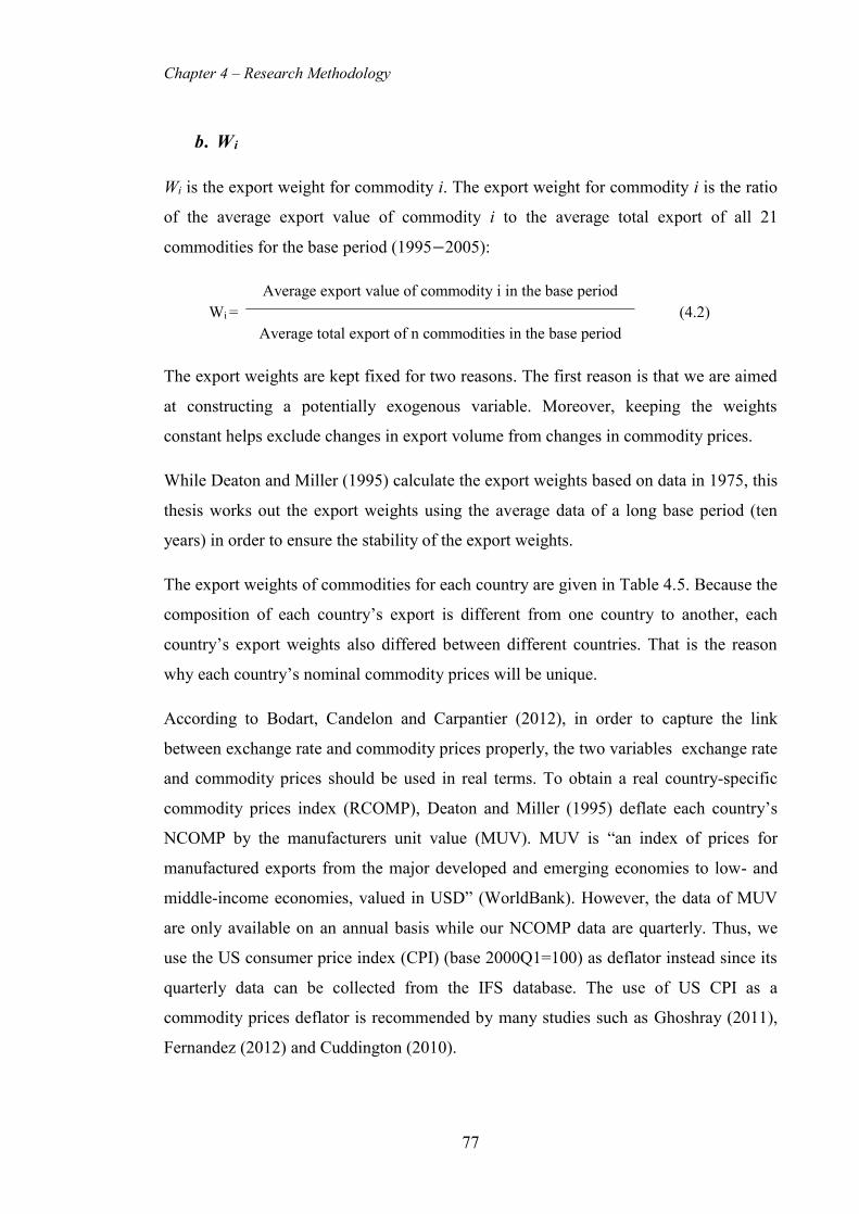
Chapter 4 – Research Methodology
77
b. W i
Wi is the export weight for commodity i. The export weight for commodity i is the ratio
of the average export value of commodity i to the average total export of all 21
commodities for the base period (1995−2005):
The export weights are kept fixed for two reasons. The first reason is that we are aimed
at constructing a potentially exogenous variable. Moreover, keeping the weights
constant helps exclude changes in export volume from changes in commodity prices.
While Deaton and Miller (1995) calculate the export weights based on data in 1975, this
thesis works out the export weights using the average data of a long base period (ten
years) in order to ensure the stability of the export weights.
The export weights of commodities for each country are given in Table 4.5. Because the
composition of each country’s export is different from one country to another, each
country’s export weights also differed between different countries. That is the reason
why each country’s nominal commodity prices will be unique.
According to Bodart, Candelon and Carpantier (2012), in order to capture the link
between exchange rate and commodity prices properly, the two variables exchange rate
and commodity prices should be used in real terms. To obtain a real country-specific
commodity prices index (RCOMP), Deaton and Miller (1995) deflate each country’s
NCOMP by the manufacturers unit value (MUV). MUV is “an index of prices for
manufactured exports from the major developed and emerging economies to low- and
middle-income economies, valued in USD” (WorldBank). However, the data of MUV
are only available on an annual basis while our NCOMP data are quarterly. Thus, we
use the US consumer price index (CPI) (base 2000Q1=100) as deflator instead since its
quarterly data can be collected from the IFS database. The use of US CPI as a
commodity prices deflator is recommended by many studies such as Ghoshray (2011),
Fernandez (2012) and Cuddington (2010).
Wi = Average export value of commodity i in the base period
(4.2) Average total export of n commodities in the base period

Chapter 4 – Research Methodology
78
The RCOMP of each individual country in the period 1986 – 2014 has been shown in
Figure 4.1 to Figure 4.12.
c. Pi
Pi is the international commodity prices index for commodity i. The international
commodity prices are sourced from the IFS. From the international prices of commodity
i, we calculate Pi at time t (base 2000Q1 = 100) as follows:
Pit =Price of commodity i (t)
Price of commodity i (2000Q1)× 100 (4.3)
It is worth noting that there are three kinds of oil prices, which are Dated Brent, Dubai
Fateh and West Texas Intermediate. Oil prices used in our study are the average of these
three kinds. Similarly, the coffee prices are the average prices of Robusta and Mild
Arabica coffee.
In fact, while prices of most commodities are determined by commodity markets, in
some countries commodity prices are controlled by home-country. For example, rice
price in Malaysia is totally controlled by its government. However, the collection of
data for a specific commodity in developing countries for a large span of time is
impossible. Although international prices are able to capture the trend of commodity
prices controlled by home-country to some extent, this replacement might lead to the
bias of the nominal country-specific commodity prices index.
4.2.3 Exchange rate
As mentioned in 4.2.2, exchange rate is measured in real terms. Furthermore, we prefer
using real effective exchange rate to using real bilateral exchange rate as real effective
exchange rate can reflect the global competitiveness of a country compared with its
trade partners. Moreover, using real effective exchange rate can help avoiding possible
biases linked to the selection of base country in bilateral real exchange rate (Cashin,
Céspedes & Sahay 2004).
Real effective exchange rate (REER) is “the weighted average of a country's currency
relative to an index or basket of other major currencies adjusted for the effects of
inflation. The weights are determined by comparing the relative trade balances, in terms
of one country's currency, with each other country within the index” (Investopedia). In
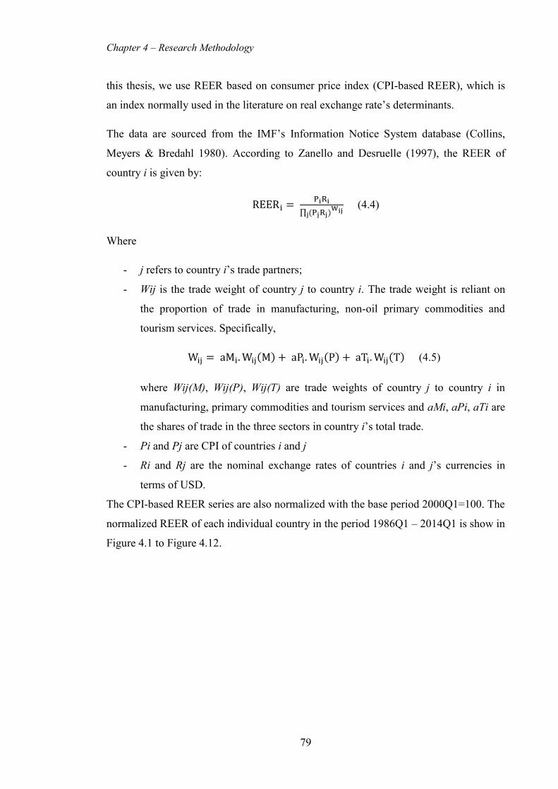
Chapter 4 – Research Methodology
79
this thesis, we use REER based on consumer price index (CPI-based REER), which is
an index normally used in the literature on real exchange rate’s determinants.
The data are sourced from the IMF’s Information Notice System database (Collins,
Meyers & Bredahl 1980). According to Zanello and Desruelle (1997), the REER of
country i is given by:
REERi = PiRi
∏ (PjRj)Wij
j
(4.4)
Where
- j refers to country i’s trade partners;
- Wij is the trade weight of country j to country i. The trade weight is reliant on
the proportion of trade in manufacturing, non-oil primary commodities and
tourism services. Specifically,
Wij = aMi. Wij(M) + aPi. Wij(P) + aTi. Wij(T) (4.5)
where Wij(M), Wij(P), Wij(T) are trade weights of country j to country i in
manufacturing, primary commodities and tourism services and aMi, aPi, aTi are
the shares of trade in the three sectors in country i’s total trade.
- Pi and Pj are CPI of countries i and j
- Ri and Rj are the nominal exchange rates of countries i and j’s currencies in
terms of USD.
The CPI-based REER series are also normalized with the base period 2000Q1=100. The
normalized REER of each individual country in the period 1986Q1 – 2014Q1 is show in
Figure 4.1 to Figure 4.12.

Chapter 4 – Research Methodology
80
Figure 4.1 – REER and RCOMP in Australia
Figure 4.2 – REER and RCOMP in Canada
0
50
100
150
200
250
300
350
400
1986
19
87
1988
19
89
1990
19
91
1992
19
93
1994
19
95
1996
19
97
1998
19
99
2000
20
01
2002
20
03
2004
20
05
2006
20
07
2008
20
09
2010
20
11
2012
20
13
2014
Bas
e 20
00Q
1 =
100
AUSTRALIA
REER
RCOMP
0
50
100
150
200
250
300
350
1986
19
87
1988
19
89
1990
19
91
1992
19
93
1994
19
95
1996
19
97
1998
19
99
2000
20
01
2002
20
03
2004
20
05
2006
20
07
2008
20
09
2010
20
11
2012
20
13
2014
Bas
e 20
00Q
1 =
100
CANADA
REER
RCOMP

Chapter 4 – Research Methodology
81
Figure 4.3 – REER and RCOMP in Iceland
Figure 4.4 – REER and RCOMP in New Zealand
0
50
100
150
200
250
300
350
1986
19
87
1988
19
89
1990
19
91
1992
19
93
1994
19
95
1996
19
97
1998
19
99
2000
20
01
2002
20
03
2004
20
05
2006
20
07
2008
20
09
2010
20
11
2012
20
13
2014
Bas
e 20
00Q
1 =
100
ICELAND
REER
RCOMP
0
20
40
60
80
100
120
140
160
180
1986
19
87
1988
19
89
1990
19
91
1992
19
93
1994
19
95
1996
19
97
1998
19
99
2000
20
01
2002
20
03
2004
20
05
2006
20
07
2008
20
09
2010
20
11
2012
20
13
2014
Bas
e 20
00Q
1 =
100
NEW ZEALAND
REER
RCOMP

Chapter 4 – Research Methodology
82
Figure 4.5 – REER and RCOMP in Norway
Figure 4.6 – REER and RCOMP in Greece
0
50
100
150
200
250
300
350
400
1986
19
87
1988
19
89
1990
19
91
1992
19
93
1994
19
95
1996
19
97
1998
19
99
2000
20
01
2002
20
03
2004
20
05
2006
20
07
2008
20
09
2010
20
11
2012
20
13
2014
Bas
e 20
00Q
1 =
100
NORWAY
REER
RCOMP
0
20
40
60
80
100
120
140
160
180
1986
19
87
1988
19
89
1990
19
91
1992
19
93
1994
19
95
1996
19
97
1998
19
99
2000
20
01
2002
20
03
2004
20
05
2006
20
07
2008
20
09
2010
20
11
2012
20
13
2014
Bas
e 20
00Q
1 =
100
GREECE
REER
RCOMP

Chapter 4 – Research Methodology
83
Figure 4.7 – REER and RCOMP in Brunei
Figure 4.8 – REER and RCOMP in Laos
0
50
100
150
200
250
300
350
400
450
1992
19
93
1994
19
95
1996
19
97
1998
19
99
2000
20
01
2002
20
03
2004
20
05
2006
20
07
2008
20
09
2010
20
11
2012
20
13
2014
Bas
e 20
00Q
1 =
100
BRUNEI
REER
RCOMP
0
20
40
60
80
100
120
140
160
180
200
1993 1994 1995 1996 1997 1998 1999 2000 2001 2002 2003 2004 2005 2006 2007 2008 2009 2010 2011 2012 2013 2014
Bas
e 20
00Q
1 =
100
LAOS
REER
RCOMP

Chapter 4 – Research Methodology
84
Figure 4.9 – REER and RCOMP in Malaysia
Figure 4.10 – REER and RCOMP in Myanmar
0
50
100
150
200
250
300
1986
19
87
1988
19
89
1990
19
91
1992
19
93
1994
19
95
1996
19
97
1998
19
99
2000
20
01
2002
20
03
2004
20
05
2006
20
07
2008
20
09
2010
20
11
2012
20
13
2014
Bas
e 20
00Q
1 =
100
MALAYSIA
REER
RCOMP
0
100
200
300
400
500
600
1986
19
87
1988
19
89
1990
19
91
1992
19
93
1994
19
95
1996
19
97
1998
19
99
2000
20
01
2002
20
03
2004
20
05
2006
20
07
2008
20
09
2010
20
11
2012
20
13
2014
Bas
e 20
00Q
1 =
100
MYANMAR
REER
RCOMP

Chapter 4 – Research Methodology
85
Figure 4.11 – REER and RCOMP in Thailand
Figure 4.12 – REER and RCOMP in Vietnam
0
50
100
150
200
250
1986
19
87
1988
19
89
1990
19
91
1992
19
93
1994
19
95
1996
19
97
1998
19
99
2000
20
01
2002
20
03
2004
20
05
2006
20
07
2008
20
09
2010
20
11
2012
20
13
2014
Bas
e 20
00Q
1 =
100
THAILAND
REER
RCOMP
0
100
200
300
400
500
600
700
800
900
1988
1989
1990
1991
1992
1993
1994
1995
1996
1997
1998
1999
2000
2001
2002
2003
2004
2005
2006
2007
2008
2009
2010
2011
2012
2013
2014
Bas
e 20
00Q
1 =
100
VIETNAM
REER
RCOMP

Chapter 4 – Research Methodology
86
4.2.4 Real interest rate
The real interest rate (RIR) is the rate of interest an investor expects to receive after
allowing for inflation. RIR is still regarded as the growth rate of purchasing power
derived from an investment.
To get the real interest rate, we take the nominal interest rate and subtract the
anticipated inflation rate. However, because the anticipated inflation rate cannot be
observed, we replace it by the inflation rate.
RIRt = it − πt (4.6)
where 𝑖 is the nominal interest rate and 𝜋 is the inflation rate
The data of the nominal interest rates (i) are obtained from the IFS. Among the several
categories of interest rates available in the IFS database, we choose three-month Deposit
Rates because of data availability. Although the risk-free Treasury Bill Rates are the
most widely used interest rate, they are not chosen as the data are not available for some
countries in the period from 1986Q1 to 2014Q1.
The inflation rate (𝜋) is the growth rate of the Consumer Price Index (CPI). The formula
for calculating the inflation rate is:
πt =CPIt−CPIt−1
CPIt−1 (4.7)
The quarterly data of CPI is sourced from the IFS database.
The two variables REER and RCOMP are employed with their natural logarithm form.
For RIR, the logarithm form is only used if they are positive (their original forms are
used otherwise). Using the logarithm transformation can be a good approach to reduce
heteroskedasticity. Moreover, OLS regression assumes that the errors, as estimated by
the residuals, are normally distributed. When they are positively skewed (long right
tail), taking the logarithm is able to help solve this problem.
Chapter 4 – Research Methodology
87
4.3 Methodology
In this thesis, we employ both time-series and panel-data techniques to investigate the
relationship between REER and RCOMP. While the time-series technique helps
provide insight into the relationship of individual countries, the panel-data technique
enables us to achieve common findings about the relationship between REER and
RCOMP for each group of developed and developing countries, which facilitate the
comparison between the two groups. Moreover, panel-data technique can overcome
limitations of time series technique. The combination of the two techniques is necessary
for our comparison.
4.3.1 Time-series technique
A three-stage procedure was followed to examine the relationship between REER and
RCOMP for each country.
4.3.1.1 Unit root tests
We first check whether the data series used in our model are stationary or not. There are
several reasons why the stationary of data series is of great importance. Firstly, the use
of non-stationary data can lead to spurious regressions. The phenomenon of spurious
regression might occur when we make regression of a non-stationary variable on
another non-stationary variable. The result looks good under standard measures
(significant coefficient estimates and a high R2) even though the two variables may be
totally unrelated. Misspecification can also arise when only one of the two variables has
a unit root. Secondly, as we will use either VAR model or VECM model to explore the
relationship between exchange rate, commodity prices, and interest rate, all variables to
be included in the VAR model or VEC model are required to be stationary in order to
carry out joint significance tests on the lags of the variables. Finally, if both series
contain unit roots but are cointegrated then the OLS estimation method is not
appropriate. For these reasons, it is important to check for unit roots in the series before
estimating a model. Augmented Dickey – Fuller (ADF) and Philips – Perron (PP) unit
root tests were adopted for this analysis.

Chapter 4 – Research Methodology
88
a. Augmented Dickey – Fuller (ADF)
The Augmented Dickey – Fuller test (ADF) is a unit root test proposed for time series
data. This test is an augmented version of the Dickey – Fuller test (Eviews 2013). The
Dickey – Fuller test is only applicable if variables are correlated at order one.
The Dickey – Fuller test uses a simple AR(1) model:
∆𝑦𝑡 = 𝛼𝑦𝑡−1 + 𝑥𝑡𝛿 + 𝑣𝑡 (4.8)
Dickey – Fuller test constructs a parametric autoregression for order 1. In the case when
variables are correlated at higher order lags, the Dickey – Fuller test is not valid since
the assumption of white noise disturbances is violated (Eviews 2013).
The ADF test use a parametric autoregression for higher order by including p lagged
difference terms to the regression. In this study, we specify the lag length (p) according
to Akaike’s information criterion (AIC). The ADF test is carried out by estimating the
following regression:
∆𝑦𝑡 = 𝛼𝑦𝑡−1 + 𝑥𝑡𝛿 + 𝛽1∆𝑦𝑡−1 + 𝛽2∆𝑦𝑡−2 + ⋯ + 𝛽𝑛∆𝑦𝑡−𝑛 + 𝑣𝑡 (4.9)
The null hypothesis: 𝛼 = 0
The alternative hypothesis: 𝛼 < 0
To test the hypothesis, the test statistic DF value is calculated:
𝐷𝐹 = �̂�
𝑆𝐸(�̂�) (4.10)
If the test statistic DF is less than the relevant critical value for the ADF test, the null
hypothesis is rejected. It can be concluded that the variable has no unit root. And, vice
versa, if the test statistic DF is larger than the relevant critical value, the null hypothesis
cannot be rejected and the variable has a unit root. For more information about ADF
unit root test, see Said and Dickey (1984).
b. Philips–Perron (PP)
The Phillips – Perron (PP) test is also based on the Dickey – Fuller test which tests the
null hypothesis 𝛼 = 0 in Equation (4.8). Similar to the ADF unit root test, the PP test
also solves the problem of low order of autocorrelation in Dickey – Fuller test (Eviews
2013).

Chapter 4 – Research Methodology
89
While the ADF test addresses the problem by adding lags of first difference to the
regression, the PP test modifies the t-test statistic of a coefficient in the Dickey – Fuller
test so that serial correlation does not affect the asymptotic distribution of the test
statistic. The modified t-test statistic of PP test:
𝑡�̃� = 𝑡𝛼(𝛾0
𝑓0)
1
2 −𝑇(𝑓0−𝛾0) (𝑠𝑒(�̂�))
2 𝑓1/20 𝑠
(4.11)
𝑠𝑒(�̂�) is coefficient standard error, s is the standard error of test regression, 𝛾0 is a
consistent estimate of the error variance, and 𝑓0 is an estimator of the residual spectrum
at frequency zero (Eviews 2013). For more details about PP test see Phillips and Perron
(1988).
4.3.1.2 Johansen (1988) cointegration test
It is widely known that nonstationary time-series should not be used in regression
models to avoid the problem of spurious regression (Gujarati 2009). However, if
variables are nonstationary but integrated of the same order and the linear combination
of variables integrated of a lower order, their regression model is still meaningful. In
this case, variables are cointegrated. In other words, variables are cointegrated if there is
a long-run or equilibrium relationship between them (Gujarati 2009).
Based on the result of unit root tests, we conduct a Johansen (1988) cointegration test to
check for cointegration between the two variables (REER an RCOMP) of the same
integration order. This is the superior test for cointegration as it has all desirable
statistical properties (Sjö 2008). The Johansen (1988) test approaches the testing for
cointegration by examining the number of independent linear combinations (k) for an m
time series variables set that yields a stationary process. The Johansen (1988) test has
two forms: the trace test and the maximum eigenvalue test.
It is worth noticing that when using Eviews software to run a Johansen (1988)
cointegration test, the lag length for Johansen (1988) cointegration testing is the lag
length for VAR model between REER and RCOMP minus one.
a. Trace Test
The trace test examines the quantity of linear combinations k to be equal to a given
value k0, and the alternative hypothesis for k to be greater than k0.

Chapter 4 – Research Methodology
90
Null hypothesis H0: k = k0
Alternative hypothesis H1: k > k0
To test whether the cointegration exists using the trace test, we set k0 = 0 (no
cointegration) and examine whether the null hypothesis can be rejected. If this is the
case, then we conclude there is at least one cointegration relationship.
b. Maximum Eigenvalue Test
For the maximum eigenvalue test, the difference is in an alternate hypothesis:
Null hypothesis H0: k = k0
Alternative hypothesis H1: k = k0 + 1
So, starting with k0 = 0 and rejecting the null hypothesis implies that there is only one
possible combination of the non-stationary variables to yield a stationary process. What
if we have more than one? The test may be less powerful than the trace test for the
same k0 values. A special case for using the maximum eigenvalue test is when k0 = m –
1, where rejecting the null hypothesis implies the existence of m possible linear
combinations. This is impossible, unless all input time series variables are stationary to
start with.
4.3.1.3 Cointegrating equation
If there is evidence of cointegration between REER and RCOMP we estimate the long-
run equilibrium relationship between them (Equation (4.12)) by using the OLS method.
REERit = α + β RCOMPit + ε1it (4.12)
The coefficient β measures the long-run elasticity of REER with respect to RCOMP. It
can be understood that a 1% increase in RCOMP is associated with 𝛽% change in
REER.
4.3.1.4 Granger causality
Granger causality is a statistical concept which is based on prediction. The starting point
of the Granger causality test is that the future cannot cause the past or present, whereas
the past may cause the present or the future (Granger 1969). Granger causality between

Chapter 4 – Research Methodology
91
two variables cannot be interpreted as a real causal relationship. If Xt is said to Granger-
cause Yt, then past values of Xt should contain information that helps predict Yt better
and beyond the information contained in past values of Yt alone.
Granger causality was developed by Granger in 1969 and has been widely used in the
literature on economics. Our thesis will investigate the Granger causality between
REER and RCOMP in developing commodity-exporting countries and developed ones
in order to identify the direction of Granger causality between REER and RCOMP.
To examine the Granger causality between REER and RCOMP, we use a three-step
procedure. The first step is building a suitable model for the purpose of Granger
causality testing, the second step is estimating the model, and the final step is testing the
hypotheses to determine the existence as well as the direction of Granger causality
between the two series in our model.
a. Building model for Granger causality testing
As mentioned in section 4.1, in order to get more precise results, we consider including
a control variable, which is RIR, when investigating the Granger causality between
REER and RCOMP.
As the direct Granger test only assumes two variables, in order to control for the effect
of another variable, we can use either a VAR or VEC model instead. The selection is
determined by the cointegration between REER and RCOMP.
- REER and RCOMP are not cointegrated
In case REER and RCOMP are not cointegrated, a vector autoregression (VAR) model
is estimated to test for Granger causality between REER and RCOMP. In our thesis, we
employ the Toda and Yamamoto (1995) augmented VAR model instead of the
traditional VAR model. The reason is that in the Toda and Yamamoto (1995)
augmented VAR model, all variables are used in level, regardless of their orders
of integration. We must not take the difference of the variables even when variables are
not stationary. Meanwhile, in a traditional VAR model, all variables are required to be
stationary. In the case that there is any variable not stationary (i.e., I(1) or I(2)), we must
differentiate that variable to make sure it is stationary in the VAR model. However,

Chapter 4 – Research Methodology
92
using variables in difference makes the results become not intuitively interpretable.
Moreover, the Granger causality between differenced variables is not what we expect.
Apart from REER and RCOMP, we also include the control variable RIR in the Toda
and Yamamoto (1995) augmented VAR model when investigating the Granger
causality between REER and RCOMP. The model is as follows:
REERt = α1 + ∑ β11kRCOMPt−k + ∑ β11(k+m)RCOMPt−(k+m)m1 + ∑ β12kREERt−k +k
1k1
∑ β12(k+m)REERt−(k+m)m1 + ∑ β13kRIRt−k
k1 + u1t (4.13)
RCOMPt = α2 + ∑ β21kREERt−k + ∑ β21(k+m)REERt−(k+m)m1 + ∑ β22kRCOMPt−k +k
1k1
∑ β22(k+m)RCOMPt−(k+m)m1 + ∑ β23kRIRt−k
k1 + u2t (4.14)
where i=1,2,…N; t=1,2,…T; 𝛼 is the interecepts; 𝛽 is the parameters; k is the lag
length; m is the maximum order of integration of REER and RCOMP; and u denotes
white-noise error terms.
Lag length (k) is the number of lagged values of the series included in the model. It is
critical to select a correct lag length for VAR. While too short a lag length fails to
reflect the system’s dynamics and leads to omitted variable bias, too long a lag length
suffers from a loss of degrees of freedom which results in over-parameterization
(Gujarati 2009). Rather than randomly selecting a lag length, it is better to depend on
selection criteria to decide the number of lags. In our model, we employ the most
common criteria – Akaike Information Criterion (AIC) – to select the appropriate lag
length k.
Based on the result of ADF and PP unit root tests, we can determine the order of
integration of each variable – REER and RCOMP. From the integration results, the
maximum order of integration of the two variables (m) is specified. For example, if one
is found to be integrated of order two (I(2)), and the other is integrated of order one I(1),
than the maximum order of integration will be two (m=2).
It must be guaranteed that there is no serial correlation in the residuals of the VAR
model. In case there is serial correlation, the lag length k should be increased until the
serial correlation disappears.

Chapter 4 – Research Methodology
93
- REER and RCOMP are cointegrated
According to Engle and Granger (1987), if there is cointegration between the two
variables, then Granger causality must exist between them in at least one direction.
Once we determine that REER and RCOMP are cointegrated, we perform a vector error
correction model (VEC) to clarify the Granger causality direction. In the presence of
cointegration between variables, although the Toda and Yamamoto (1995) augmented
VAR model can be used to specify the Granger causality, a VEC model is believed to
be superior to a VAR model. Specifically, a VAR model is only able to determine short-
run Granger causality. Meanwhile, VEC model which is capable of identifying both
short-run and long-run relationships among variables as well as determining the sources
of causation36 (Oh & Lee 2004). In line with this finding, Asafu-Adjaye (2000) also
claims that the a VEC model has created a long-run causality channel that is overlooked
by the traditional Granger causality test (Granger 1969).
We also include the control variable RIR in the VEC model when investigating the
Granger causality between REER and RCOMP. The following VEC model is
considered:
∆REERt = α1 + β10ECT1,t−1 + ∑ β11k∆RCOMPt−k + ∑ β12k∆REERt−k + ∑ β13k∆RIRt−kk +kk
u1t (4.15)
∆RCOMPt = α2 + β20ECT2,t−1 + ∑ β21k∆REERt−k + ∑ β22k∆RCOMPt−k + ∑ β23k∆RIRt−kk +kk
u2t (4.16)
where ECT is an error correction term. ECTt-1 is “the measure of the extent by which
the observed values in time t–1 deviate from the long-run equilibrium relationship”
Costantini and Martini (2010). ECT1,t-1 and ECT2,t-1 are both stationary.
ECT1,t-1 is the first lagged value of the residuals derived from the cointegration
regression of the two variables REER and RCOMP for which REER is a dependent
variable (see Equation (4.17)). And, ECT2,t-1 is the first lagged value of the residuals
from the cointegration regression of the two variables RCOMP and REER for which
RCOMP is a dependent variable (see Equation (4.18)).
36 The term “Granger causality” always implies a short-term relationship (Gujarati 2009). The term “short-run Granger causality” is only used to easily distinguish “Granger causality” from “long-run Granger causality”.

Chapter 4 – Research Methodology
94
REERt = γ1 + δ1RCOMPt + ε1t (4.17)
RCOMPt = γ2 + δ2REERt + ε2t (4.18)
In order to obtain ECT1,t-1 and ECT2,t-1, we prefer using an OLS to estimate Equations
(4.17) and (4.18). The coefficients 𝛽10, 𝛽20 of the ECTs represent the deviation of the
dependent variables from the long-run equilibrium.
b. Estimating models
In order to estimate the Toda and Yamamoto (1995) augmented VAR model and VEC
model, we use the ordinary least square (OLS) equation by equation.
c. Checking for serial correlation
Before testing hypotheses to specify the Granger causality between variables, we should
test for serial correlation of VAR or VEC model. According to Giles (2011), a serial
correlation test should be a pre-test for Granger causality, while heteroskedasticity and
normality testing are not really necessary.
In the presence of serial correlation, coefficients estimated by OLS are still unbiased but
are inefficient, even at large sample sizes. As a result, the standard error will be wrong
which in turn leads to incorrect Granger causality test results.
In order to test for serial correlation of our VAR and VECM models, we apply the
Breusch – Godfrey Lagrange multiplier test (LM test). This is because a LM test is able
to test for autocorrelation of any order and suitable for the models with lagged
dependent variables.
To guarantee the reliability of a Granger test result, there should be no serial correlation
in the VAR or VEC model. In case there is serial correlation in the model, lag length
will be increased until the serial correlation disappears.
d. Testing Granger causality
We determine the direction of Granger causality by testing for the significance of the
dependent variables’ coefficients in the equations of the VAR or VEC model.

Chapter 4 – Research Methodology
95
- REER and RCOMP are not cointegrated
In the case where there is no cointegration between REER and RCOMP, short-run
causality between REER and RCOMP is investigated based on the estimation result of
the Toda and Yamamoto (1995) augmented VAR model.
In order to detect whether there is Granger causality running from RCOMP and RIR to
REER, we test the joint significance of the coefficients of k lagged values of RCOMP
(β111, β112, … , β11k) and RIR (β131, β132, … , β13k) in Equation (4.13). It is worth noting that
the extra m lags of RCOMP are not included when performing the test for joint
significance of coefficients.
Similarly, to determine if there is Granger causality running from REER and RIR to
RCOMP, we test the joint significance of the coefficients of k lagged values of REER
(β211, β212, … , β21k) and RIR (β231, β232, … , β23k) in Equation (4.14).
Specifically, to determine whether the causality runs from RCOMP to REER, we use a
Wald test of the null hypothesis based on Equation (4.13) as follows:
Null hypothesis H0: β111 = β112 = … = β11k = 0 against
Alternative hypothesis H1: At least one β11j ≠ 0 j = 1, 2, …, k
To determine whether the causality runs from RIR to REER, we use a Wald test to test
the null hypothesis based on Equation (4.13) as follows:
Null hypothesis H0: β131 = β132 = … = β13k = 0 against
Alternative hypothesis H1: At least one β13j ≠ 0 j = 1, 2, …, k
Similarly, to determine whether causality runs from REER to RCOMP, we test the null
hypothesis for Equation (4.14) as follows:
Null hypothesis H0: β211 = β212 = … = β21k = 0 against
Alternative hypothesis H1: At least one β21j ≠ 0 j = 1, 2, …, k
To determine whether causality runs from RIR to RCOMP, we test the null hypothesis
for Equation (4.14) as follows:

Chapter 4 – Research Methodology
96
Null hypothesis H0: β231 = β232 = … = β23k = 0 against
Alternative hypothesis H1: At least one β23j ≠ 0 j = 1, 2, …, k
If the null hypothesis is rejected, it can be concluded that there is Granger causality in
that direction and vice versa. In other words, the rejection of the null hypothesis proves
the presence of Granger causality.
- REER and RCOMP are cointegrated
In the case where the cointegration between REER and RCOMP is found, Granger
causality between REER and RCOMP is investigated based on a VEC model.
Accordingly, Granger causality is sub-divided into long-run and short-run Granger
causality.
Short-run Granger causality
For a VEC model, the short-run causality between variables can be done in the same
manner as in a VAR model. We also use a Wald test to test for the joint hypothesis of
the first difference of k lagged explanatory variables. Based on Equation (4.15), we test
the following null hypothesis to check if there is any Granger causality running from
RCOMP to REER:
Null hypothesis H0: β111 = β112 = … = β11k = 0 against
Alternative hypothesis H1: At least one β11j ≠ 0 j = 1, 2, …, k
And, the following null hypothesis is tested based on Equation (4.15) to see if there is
any Granger causality running from RIR to REER:
Null hypothesis H0: β131 = β132 = … = β13k = 0 against
Alternative hypothesis H1: At least one β13j ≠ 0 j = 1, 2, …, k
Identically, to detect whether causality run from REER to RCOMP we test the null
hypothesis based on Equation (4.16):
Null hypothesis H0: β211 = β212 = … = β21k = 0 against
Alternative hypothesis H1: At least one β21j ≠ 0 j = 1, 2, …, k

Chapter 4 – Research Methodology
97
And, testing the following null hypothesis based on Equation (4.16) is to determine if
there is any Granger causality running from RIR to RCOMP:
Null hypothesis H0: β231 = β232 = … = β23k = 0 against
Alternative hypothesis H1: At least one β23j ≠ 0 j = 1, 2, …, k
If the null hypothesis is rejected, it can be concluded that there is Granger causality in
that direction and vice versa. In other words, the rejection of the null hypothesis proves
the presence of Granger causality.
Long-run Granger causality
Long-run causality is determined by the coefficients of ECTt-1 in the VEC model. If
ECTt-1’s coefficients are significant and have proper sign, it can be concluded that there
is evidence of long-run causality from the explanatory variable to the dependent
variable. Particularly, if β10 in Equation (4.15) is statistically significant and negative
(β10< 0), there will be a long-run causality running from RCOMP to REER.
And, if β20 in Equation (4.16) is significant and has an appropriate sign, there will be a
long-run causality running from REER to RCOMP. The expected sign of β20 depends
on the sign of β in Equation (4.12). Specifically, it is expected that the sign of β20 can
satisfy the requirement of − β20∙ β < 0 (Johansen 1995).
4.3.2 Panel-data technique
Apart from the time-series technique applied for individual countries, we also employ
panel-data technique to examine the relationship for each group: six OECD and six
ASEAN countries. The panel data set is one that provides observations over time for a
sample of individuals (Hsiao 2003). In order to facilitate the comparison of the
relationship between commodity prices and exchange rate between developed and
developing countries, two panel data sets are built: one for the group of six OECD
commodity-exporting countries and one for the group of six ASEAN commodity-
exporting countries.
There are some reasons explaining the employment of panel-data technique in our
thesis. The most important reason is that panel-data technique can be used effectively in
achieving common findings about the commodity prices – exchange rate nexus for a

Chapter 4 – Research Methodology
98
whole group of countries. These common findings will enable us to compare the real
commodity prices – real exchange rate relationship between the two groups of countries
without any difficulties. The panel-data technique will become especially useful for
comparison when the result of the time series tests show the differences in relationship
from country to country.
In addition, the panel-data technique is also superior to time-series technique in some
aspects. First, panel data gives considerably more informative data, variability, degree
of freedom, and less collinearity among variables compared to cross-sectional data and
time-series data because panel data is the combination of both kinds of data (Gujarati
2009). Second, by using panel-data technique we can avoid problems of low power
associated with the time-series tests, especially the traditional cointegration test and unit
root test. With a great increase in the number of observations, the panel cointegration
test has a higher power compared to the traditional one (Rapach & Wohar 2004). The
traditional unit root tests are said to be notorious for their low power (see Cochrane
(1991), DeJong et al. (1992), Maddala and Kim (1998)). Hatanaka (1996) also points
out that with sample size 100, characteristic roots between 0.9 and 1.0 cannot be
distinguished from a unit root.
On the whole, using panel data helps facilitate the comparison between developing
countries and developed countries, which is the main aim of our thesis. Moreover,
panel-data techniques can overcome the limitations of time-series technique. Therefore,
a combination of time-series technique and the panel-data technique can help provide a
reliable and comprehensive insight into the relationship between real commodity prices
and real exchange rate in both developed and developing countries which forms a firm
foundation for comparison.
When applying panel-data technique, the testing process is similar to that of time-series
technique. First, we use a panel data unit root tests to check the stationarity of variables
in each group of countries. If the REER and RCOMP are integrated of same order, we
run the panel cointegration test to see if there is long-run relationship between the two
variables in each group of countries and estimate the long-run commodity price
elasticity of real exchange rate. Finally, we test for the Granger causality between
REER and RCOMP based on panel Toda and Yamamoto (1995) augmented VAR or
VEC model.

Chapter 4 – Research Methodology
99
4.3.2.1 Panel unit root tests
Panel unit root tests are believed to be more powerful than traditional unit root tests on
individual time series (Rapach & Wohar 2004) . Since Levin and Lin (1992) unit root
tests, there have been many various panel data unit root tests proposed. However, the
most popular panel unit tests in practice are Levin, Lin and Chu (2002), Breitung
(2000), Hadri (2000), Maddala and Wu (1999), Im, Pesaran and Shin (2003), and Choi
(2001).
The general structure used by most (though not all) panel unit root testing procedures is:
∆yit = αiyi,t−1 + ∑ ∆yit−jpij=1 + X′itδ + ϵit (4.19)
where
- Pi is the lag length for the difference terms, which varies across individuals
- Xit represent the exogenous variables in the model
- 𝜀it refers to the error terms
- If 𝛼𝑖 < 0, yi is weakly stationary. On the other hand, if 𝛼𝑖 = 0 then yi contains a
unit root.
Among the six panel unit root tests mentioned above, there are two natural assumptions
about the 𝛼 used. While Levin, Lin and Chu (2002) (LLC), Breitung (2000), and Hadri
(2000) panel unit root tests all assume that the parameters are the same across cross-
sections so that 𝛼𝑖 = 𝛼 for all i, Im, Pesaran and Shin (2003), Maddala and Wu (1999)
and Choi (2001) allow 𝛼𝑖 to vary freely across cross-sections.
In our thesis, we only use heterogeneous panel unit root tests which allow for the slope
heterogeneity as those of Im, Pesaran and Shin (2003), Maddala and Wu (1999) and
Choi (2001). These heterogeneous panel unit root tests are the most suitable for our
study because heterogeneity could stem from different economic conditions of
individual countries.
a. Im, Pesaran and Shin (2003) test
The Im, Pesaran and Shin (2003) panel unit root test starts by estimating an augmented
Dickey-Fuller (ADF) regression for each cross-section:

Chapter 4 – Research Methodology
100
∆yit = αiyi,t−1 + ∑ ∆yit−jpij=1 + X′itδ + ϵit (4.20)
Null hypothesis: H0: 𝛼𝑖 = 0 for all i
Alternative hypothesis: H1: 𝛼𝑖 = 0 for i = 1, 2, 3, ..., N1
𝛼𝑖 < 0 for i = N1, N2, ..., N
After estimating the regression (4.18), the average of the t-statistics is calculated as
follows:
tN,T̅̅ ̅̅ ̅ = 1
N ∑ ti,T
Ni=1
√NtN,T̅̅ ̅̅ ̅ − μ
σ~N(0,1)
where E(ti,T) = μ and V(ti,T) = σ2
The test assumes that T is the same for all cross-section units. Therefore, the Im,
Pesaran and Shin (2003) test is only applied for balanced panel data.
b. Maddala and Wu (1999) test
Maddala and Wu (1999) panel unit root test uses the Fisher (𝑝𝜆) test which is based on
gathering the p-values of the test-statistic for a unit root in each cross-section.
Similar to the Im, Pesaran and Shin (2003) test, the null and alternative hypotheses are
as follows:
Null hypothesis: H0: 𝛼𝑖 = 0 for all i
Alternative hypothesis: H1: 𝛼𝑖 = 0 for i = 1, 2, 3, ..., N1
𝛼𝑖 < 0 for i = N1, N2, ..., N
Under the null hypothesis of unit root for all cross-sections, we have the asymptotic
result that:
pλ = −2 ∑ logeπiNi=1 ~χ2N
2 .
where 𝜋i is the p-value from unit root test for each cross-section, which is derived from

Chapter 4 – Research Methodology
101
the distribution of ADF t-statistics by Monte-Carlo simulation,
After the Fisher-test statistics are computed, we compare the Fisher-test statistics with
the appropriate 𝜒2critical value.
One advantage of the Maddala and Wu (1999) test is that it can be applied to an
unbalanced panel. However, the shortcoming of the Maddala and Wu (1999) test is that
the p-values for each cross-section have to be obtained by Monte-Carlo simulation.
However, with the support of available computer software, the application of Maddala
and Wu (1999) test is no longer a problem.
c. Choi (2001) test
The Choi (2001) panel unit root also proposes a Fisher test like Maddala and Wu (1999)
test. Especially, when N is large, Choi (2001) proposes a Z test:
Z = −1
√N∑ (lnπi + 1)N
i=1
Assuming that the p-value of a unit root test for cross-section i is independent and
identically distributed, and using the Lindeberg – Levy central limit theorem gives the
null hypothesis Z ~ N (0, 1) as Ti → ∞ followed by N → ∞.
The adoption of the three heterogeneous panel unit root tests mentioned in this section
can overcome the deviation created by any single method. All three panel unit root tests
are applied in both panel data sets – OECD and ASEAN commodity-exporting
countries in order to test for the stationary of the three variables REER, RCOMP and
RIR. Specifically, through the panel unit root test results, we can determine if these
variables are stationary or integrated of order one (I(1)) or integrated of order two (I(2)).
4.3.2.2 Panel cointegration test
According to Granger (1981), it is believed that if the variables become stationary after
being first-differenced (or integrated of order one I(1)), it is evidence that they are
possibly cointegrated. Therefore, if the results from panel unit root tests imply that
variables are I(1), what should be done next is to use panel cointegration tests to check
if there exists a long-run relationship among the variables. A cointegration test can be
considered as a “pre-test to avoid spurious regression” (Gujarati 2009).

Chapter 4 – Research Methodology
102
Among existing panel cointegration tests, the most widely used ones are Kao (1999)
and Pedroni (1999) tests. In our thesis, to determine whether a cointegrating relationship
exists between REER and RCOMP, we employ the Pedroni (1999) test as it allows for
heterogeneous intercepts and trend coefficients across cross-sections.
A Pedroni (1999) panel cointegration test is based on a unit root in the residuals of the
cointegrating regression. If the residuals are I(0), it can be concluded that the variables
are cointegrated. On the other hand, if the residuals are I(1), the variables are not
cointegrated.
In a Pedroni (1999) panel unit root test, the cointegrating regression is first estimated
independently for each cross-section. Then, the residuals obtained from the regression
are pooled in order to conduct the panel tests.
First, the following cointegrating regression is estimated for each cross-section:
Yit = αi + δit + β1ix1i,t + β2ix2i,t + ⋯ + βMixMi,t + εit (4.21)
Assuming that y and x1,…, xM are I(1). The parameters 𝛼𝑖 are individual effects and 𝛿𝑖
are trend effects.
The null hypothesis is no cointegration among variables or the residuals of the
cointegrating regression is I(1). To test for the null hypothesis, we test whether the
residuals obtained from (4.21) are I(1) by estimating the secondary regression for each
cross-section.
𝜀𝑖𝑡 = 𝛾𝑖𝜀𝑖𝑡−1 + ∑ 𝜃𝑖𝑗Δ𝜀𝑖𝑡−𝑗 +𝑝𝑖𝑗=1 𝑣𝑖𝑡 (4.22)
Now, the null hypothesis of no cointegration becomes 𝛾𝑖 = 1. In the (Pedroni 1999)
panel unit root test, there are two types of alternative hypotheses. They are homogenous
alternative and heterogeneous alternative. Specifically, there are four within-dimension
tests using homogenous alternative, (𝛾𝑖 = 𝛾 < 1 for all i) which are panel v-statistic,
panel r-statistic, panel PP-statistic, and the panel ADF-statistic. In addition, there are
three between-dimension tests using heterogeneous alternative, (𝛾𝑖 < 1 for all i) which
are the group r-statistic, group PP-statistics, and the group ADF-statistic. For the seven
test statistics, if the computed test statistics are smaller than the critical value, we reject
the null hypothesis of absence of cointegration and vice versa. If the majority of the test
Chapter 4 – Research Methodology
103
statistics cannot reject the null hypothesis of no cointegration, it can be concluded that
there is no cointegration among variables.
4.3.2.3 Panel cointegrating equation
If there is evidence of cointegration between REER and RCOMP, we estimate the long-
run equilibrium relationship between them. The panel cointegration equation is as
follows:
REERit = α + β RCOMPit + ε1it (4.23)
The coefficient β measures the long-run elasticity of REER with respect to RCOMP.
For panel framework, the most frequently used estimators of a long-run relationship are
FMOLS and DOLS. It is commonly known that utilizing OLS to estimate cointegrated
panels will lead to a biased and inconsistent estimator. Although bias-corrected OLS
can be employed to reduce the bias, it cannot perform better than the OLS estimator in
general.
In this thesis, we employ DOLS to estimate the long-run relationship between REER
and RCOMP for each group of countries. This estimator enables us to correct bias
created by endogeneity and serial correlation, which is the main problem of OLS
estimators. Besides, it is worth noting that DOLS cannot perform sufficiently well if the
number of time periods is smaller than 20 (Pedroni 2001). As in our case, each panel
data set covers 113 time periods (quarters); DOLS is therefore suitable estimator.
For a DOLS estimator, Pedroni (2001) also claims that the group-mean estimator has
smaller size distortions than the pooled panel estimator. Because of that, the group-
mean DOLS estimator is used instead of the pooled panel one. For a detailed description
of the group-mean DOLS, see Pedroni (2001).
4.3.2.4 Granger causality
a. Building models
- REER and RCOMP are not cointegrated
In the case that REER and RCOMP are not cointegrated, the panel Toda and Yamamoto
(1995) augmented VAR model is estimated to test for Granger causality between REER

Chapter 4 – Research Methodology
104
and RCOMP.
REERit = α1i + ∑ β11kRCOMPi,t−k + ∑ β11(k+m)RCOMPi,t−(k+m)m1 + ∑ β12kREERi,t−k +k
1k1
∑ β12(k+m)REERi,t−(k+m)m1 + ∑ β13kRIRi,t−k
k1 + u1it (4.24)
RCOMPit = α2i + ∑ β21kREERi,t−k + ∑ β21(k+m)REERi,t−(k+m)m1 + ∑ β22kRCOMPi,t−k +k
1k1
∑ β22(k+m)RCOMPi,t−(k+m)m1 + ∑ β23kRIRi,t−k
k1 + u2it (4.25)
where i=1,2,…N; t=1,2,…T; 𝛼 represents cross-section specific unit dummies; 𝛽 is the
parameters to be estimated; u denotes white-noise error terms; k is the lag length.
Based on the result of Im, Pesaran and Shin (2003), Maddala and Wu (1999) and Choi
(2001) panel unit root tests, we can specify the order of integration of each variable –
REER and RCOMP. Based on the order of integration, the maximum order of
integration of the two variables (m) is specified.
We also employ Akaike Information Criterion (AIC) to select the appropriate lag length
(k). And, the selected lag length must guarantee that there is no serial correlation in the
residuals of panel VAR model. In case there is serial correlation, the lag length k should
be increased until the serial correlation disappears.
One issue we have to concern is that whether time dummies should be included in our
panel VAR model. For panel data set with large N and small T, time dummies should be
included because only a small number of dummies have to be added to the model.
However, in our case, the time dimension T is large (T=113), adding time dummies
would involve a considerable loss in efficiency. Consequently, we only include cross-
section specific unit dummies in our panel VAR model.
- REER and RCOMP are cointegrated
When REER and RCOMP are cointegrated, the following panel VEC model which is
appropriate for heterogeneous panels, is considered:
∆REERit = α1i + β10ECT1i,t−1 + ∑ β11k∆RCOMPi,t−k + ∑ β12k∆REERi,t−k + ∑ β13k∆RIRi,t−kk + u1itkk (4.26)
∆RCOMPit = α2i + β20ECT2i,t−1 + ∑ β21k∆REERi,t−k + ∑ β22k∆RCOMPi,t−k + ∑ β23k∆RIRi,t−kk + u2itkk (4.27)
where ECT is an error correction term. ECTt-1 is “the measure of the extent by which
the observed values in time t-1 deviate from the long-run equilibrium relationship”

Chapter 4 – Research Methodology
105
(Costantini & Martini 2010). ECT1i,t-1 and ECT2i,t-1 are both stationary.
ECT1i,t-1 are the first lagged values of the residuals derived from the cointegration
regression of the two variables REER and RCOMP for which REER is a dependent
variable (see Equation (4.28)) and ECT2i,t-1 are the first lagged values of the residuals
from the cointegration regression of the two variables RCOMP and REER for which
RCOMP is a dependent variable (see Equation (4.29)).
REERit = γ1i + δ1RCOMPit + ε1it (4.28)
RCOMPit = γ2i + δ2REERit + ε2it (4.29)
As mentioned in Section 4.3.2.3, FMOLS and DOLS are the two common estimators
used for cointegrating equations. In order to obtain ECT1i,t-1 and ECT2i,t-1, we prefer
using DOLS to estimate Equations (4.28) and (4.29). The DOLS estimator is chosen as
it performs better than non-parametric FMOLS estimator. A DOLS estimator is
believed to be superior to other estimators including both single equation estimators and
system estimators (Wagner & Hlouskova 2009). Additionally, Harris and Sollis (2003)
also claim that “non-parametric approaches such as FMOLS are less robust if the data
have significant outliers and have problems in cases where the residuals have large
negative moving average components.” These cases are quite common in
macroeconomic series data. The coefficients 𝛽10 , 𝛽20 of the ECTs represent the
deviation of the dependent variables from the long-run equilibrium.
b. Estimating models
In order to estimate panel VAR or VEC models, there has been a wide range of
estimation methods. One of the most popular methods is the generalized method of
moments (GMM). Since the PVAR program, which supports effectively the estimation
of panel VAR models by GMM, was written by Love and Zicchino (2006), GMM has
been used more commonly. However, GMM is not chosen for estimating panel VAR or
VEC models in our thesis because of the following reasons. The first reason is that the
GMM technique have been designed for the case of a large cross-sectional dimension
(N) relative to the time dimension (T) (Juessen & Linnemann 2010). Otherwise, the
estimation result would be severely biased and imprecise (Bruno 2005a). Since in our
thesis, each panel data set has a small N (six countries) relative to T (113 quarter
periods from 1986Q1 to 2014Q1), a GMM estimator appears less suitable.

Chapter 4 – Research Methodology
106
Secondly, although GMM performs reasonably well in terms of bias, it performs poorly
in terms of root mean square error and tends to produce estimates with a large variance
(Juessen & Linnemann 2010). Especially, “if the instruments used in the instrumental
variables or GMM estimation are only weakly correlated with the instrumental
variables, this would in turn give rise to biased coefficient estimates and hypothesis
tests with large size distortions” (Stock & Yogo 2005).
For panels that are characterized by a relatively large T but a small N as typically
encountered in macroeconomic applications, Juessen and Linnemann (2010) conclude
that bias-corrected fixed effects or bias-corrected least square dummy variables
(LSDVC) is the estimator of choice for estimating a panel VAR model. However, while
LSDVC might produce superior results, it is not always practical to implement (Judson
& Owen 1999). Most studies on LSDVC – such as Kiviet (1995), Kiviet (1999), Bun
and Kiviet (2001), Bun and Kiviet (2003), and Bruno (2005a)–served the purpose of
estimating a single dynamic panel data model. Especially, Bruno (2005b) has released a
Stata program, xtlsdvc, that computes LSDVC estimators and their bootstrap variance
covariance matrix for dynamic unbalanced panel data models based on the formulas
stated by Bruno (2005a). However, an important limitation of these estimators is that
they require all regressors to be strictly exogenous. A variable is called strictly
exogenous in a particular equation if it is not related to past, current, and future errors in
that equation. Therefore, these LSDVC versions should not be applied in our panel
VAR or VEC model to test where both REER and RCOMP are treated as endogenous.
There is only one LSDVC estimator, developed by Hahn and Kuersteiner (2002) that
can be used in estimating a panel VAR model when both N and T are large. However,
because of the problems associated with the practical implementation of this approach,
they are almost never used in empirical applications.
In this thesis, we decided to use the least square dummy variable (LSDV) estimator to
estimate panel VAR or VEC. Although the LSDV is well known for yielding biased and
inconsistent estimations in panel data models, it is finally chosen for several reasons.
First, according to Nickell (1981) and Bun and Kiviet (2006), the size of the fixed-
effects bias is dependent negatively on the time dimension (N) of the panel data sate. As
in our thesis, we consider two panel data sets with a large number of observations per
cross-section unit (N=113). Therefore, in our application, bias is not a problem. In

Chapter 4 – Research Methodology
107
addition, Judson and Owen (1999) compare the performance of the LSDV with the
GMM regarding bias and root-mean-squared error of the coefficient estimates.
According to the finding, even for a modest time dimension of 30 (N = 30), the LSDV
also outperforms the GMM. Accordingly, with N = 113, the LSDV provides a more
precise estimation in comparison with what is generated by the GMM. Moreover, the
LSDV yields a relatively small variance compared to GMM (Bun & Kiviet 2001).
Because of the above-mentioned strengths, the LSDV estimator is the most widely
applied estimator in the macroeconomic panel VAR literature (Juessen & Linnemann
2010).
Following the LSDV estimator, we define a set of dummy variables Di, where Di is
equal to one in the case of an observation relating to individual i and zero otherwise.
With cross-sectional data, one would define a dummy variable for every observation,
exhausting the degrees of freedom. After defining a set of dummy variables in each
equation panel VAR or VEC model, we can use OLS to estimate the model effectively.
c. Checking for serial correlation
Serial correlation is not normally observed in time series data but is in panel data.
Therefore, before testing hypotheses to specify the Granger causality between variables,
we should test for serial correlation of panel Toda and Yamamoto (1995) augmented
VAR or panel VEC model.
Similar to time series data, in order to test for serial correlation of our panel VAR or
VEC model, we also apply the Breusch – Godfrey Lagrange Multiplier test (LM test).
To guarantee the reliability of the Granger test result, there should be no serial
correlation in these models. In case there is serial correlation in the model, lag length
will be increased until the serial correlation disappears.
d. Testing Granger causality
We determine the direction of Granger causality by testing for the significance of the
dependent variables’ coefficients in the equations of panel augmented VAR or VEC
model.

Chapter 4 – Research Methodology
108
- REER and RCOMP are not cointegrated
In the case where there is no cointegration between REER and RCOMP, short-run
causality between REER and RCOMP is investigated based on the estimation result of
the panel Toda and Yamamoto (1995) augmented VAR model.
Similar to a time-series technique, to determine whether the causality runs from
RCOMP to REER, we use a Wald test to test the null hypothesis based on Equation
(4.24) as follows:
Null hypothesis H0: β111 = β112 = … = β11k = 0 against
Alternative hypothesis H1: At least one β11j ≠ 0 j = 1, 2, …, k
To determine whether the causality runs from RIR to REER, we use a Wald test to test
the null hypothesis based on Equation (4.24) as follows:
Null hypothesis H0: β131 = β132 = … = β13k = 0 against
Alternative hypothesis H1: At least one β13j ≠ 0 j = 1, 2, …, k
Similarly, to figure out whether causality runs from REER to RCOMP, we test the null
hypothesis based on Equation (4.25) as follows:
Null hypothesis H0: β211 = β212 = … = β21k = 0 against
Alternative hypothesis H1: At least one β21j ≠ 0 j = 1, 2, …, k
To determine whether causality runs from RIR to RCOMP, we test the null hypothesis
based on Equation (4.25) as follows:
Null hypothesis H0: β231 = β232 = … = β23k = 0 against
Alternative hypothesis H1: At least one β23j ≠ 0 j = 1, 2, …, k
If the null hypothesis is rejected, it can be concluded that there is Granger causality in
that direction and vice versa. In other words, the rejection of the null hypothesis proves
the presence of Granger causality.

Chapter 4 – Research Methodology
109
- REER and RCOMP are cointegrated
In the case where the cointegration between REER and RCOMP is found, short-run and
long-run Granger causality between REER and RCOMP is investigated based on panel
VEC model.
Short-run Granger causality
We also use a Wald test to test the joint hypothesis of the first difference of k lagged
explanatory variables in the panel VEC model. Based on Equation (4.26), we test the
following null hypothesis to check if there is any Granger causality running from
RCOMP to REER:
Null hypothesis H0: β111 = β112 = … = β11k = 0 against
Alternative hypothesis H1: At least one β11j ≠ 0 j = 1, 2, …, k
And, the following null hypothesis is tested based on Equation (4.26) to see if there is
any Granger causality running from RIR to REER:
Null hypothesis H0: β131 = β132 = … = β13k = 0 against
Alternative hypothesis H1: At least one β13j ≠ 0 j = 1, 2, …, k
Identically, to detect whether causality run from REER to RCOMP, we test the null
hypothesis based on the Equation (4.27):
Null hypothesis H0: β211 = β212 = … = β21k = 0 against
Alternative hypothesis H1: At least one β21j ≠ 0 j = 1, 2, …, k
And, testing the following null hypothesis based on Equation (4.27) to determine if
there is any Granger causality run from RIR to RCOMP:
Null hypothesis H0: β231 = β232 = … = β23k = 0 against
Alternative hypothesis H1: At least one β23j ≠ 0 j = 1, 2, …, k
If the null hypothesis is rejected, it can be concluded that there is Granger causality in
that direction and vice versa.

Chapter 4 – Research Methodology
110
Long-run Granger causality
Long-run causality is determined by the coefficients of ECTt-1 in the VEC model. If
ECTt-1’s coefficients are significant and have proper sign, it can be concluded that there
is evidence of long-run causality from the explanatory variable to the dependent
variable.
Particularly, if β10 in Equation (4.26) is statistically significant and negative (β10< 0),
there will be a long-run causality running from RCOMP to REER.
And, if β20 in Equation (4.27) is significant and has an appropriate sign, there will be a
long-run causality running from REER to RCOMP. The expected sign of β20 depends
on the sign of β in Equation (4.23). Specifically, it is expected that the sign of β20 can
satisfy the requirement of −β20∙ β < 0 (Johansen 1995).
4.4 Summary
This chapter discusses the method of obtaining data for the three variables REER,
RCOMP, and RIR. Based on the collected data from 1986Q1 to 2014Q1, the chapter
also presents necessary steps to investigate the relationship between real effective
exchange rate and real commodity prices in developed and developing countries. In our
thesis, both time-series and panel-data techniques are employed. For each country, ADF
and PP unit root tests are applied to test the stationarity of variables. A Johansen (1988)
cointegration test is then used to test for long-run relationship as well as determine
cointegrating equations between REER and RCOMP in individual countries. Finally,
the Granger causality between exchange rate and commodity prices is examined based
on Toda and Yamamoto (1995) augmented VAR or VEC model.
For each group of countries, panel data unit root tests consisting of Im, Pesaran and
Shin (2003), Maddala and Wu (1999) and Choi (2001) techniques are used to test
whether the variables are stationary or not. The Pedroni (1999) panel cointegration test
is chosen in order to clarify the existence of long-run relationship between REER and
RCOMP in each group of countries. If there is a long-run relationship between
variables, the long-run commodity price elasticity of real exchange rate is estimated by
DOLS. Granger causality is tested using a panel Toda and Yamamoto (1995)

Chapter 4 – Research Methodology
111
augmented VAR or VEC model. The result of these tests will be analysed in detail in
the next chapter.

Chapter 5 – Results and discussion
112
Results and Discussion
This chapter presents results of tests listed in Chapter 4, including unit root tests,
cointegration tests, and Granger causality. Furthermore, long-run elasticity of real
exchange rate with respect to real commodity prices will be examined if real exchange
rate and commodity prices are cointegrated. Based on tests results analysis, the two
main research questions outlined in Section 1.2 will be clarified.
5.1 Test results
As mentioned in Section 4.3, the relationship between exchange rate and commodity
prices in OECD and ASEAN are investigated by both time-series and panel-data
techniques. The time-series technique is applied for individual countries and panel-data
technique is used for each group of countries.
5.1.1 Individual countries
The results of unit root tests, Johansen (1988) cointegration test and Granger causality
tests for individual countries are as follows.
5.1.1.1 Unit root tests
We apply both augmented Dickey−Fuller (ADF) and Phillips−Perron (PP) unit root
tests with trend and without trend to check the stationarity of the three variables REER,

Chapter 5 – Results and discussion
113
Table 5.1 – Unit root tests for REER, RCOMP and RIR – individual OECD countries
Country Variables Level/ First difference
ADF Test Statistic
PP Test Statistic Conclusion Without
trend With trend
Without trend
With trend
Australia
REER Level First difference
-1.14 (1) -7.33 (0)*
-1.67 (1) -7.35 (0)*
-0.56 (0) -7.12 (5)*
-1.46 (2) -7.05 (6)* I(1)
RCOMP Level First difference
-1.51 (0) -9.97 (0)*
-2.24 (0) -9.94 (0)*
-1.47 (3) -10.02 (7)*
-2.27 (2) -10.00 (8)* I(1)
RIR Level First difference
-1.39 (1) -15.32 (0)*
-2.71 (1) -15.27 (0)*
-1.49 (5) -17.81 (9)*
-3.78 (4)* -17.81 (9)* I(1)
Canada
REER Level First difference
-1.31 (2) -7.97 (1)*
-1.32 (2) -7.94 (1)*
-1.49 (4) -8.34 (3)*
-1.50 (4) -8.30 (3)* I(1)
RCOMP Level First difference
-1.01 (0) -8.94 (1)*
-2.03 (0) -8.97 (1)*
-0.94 (2) -10.37 (4)*
-2.08 (1) -10.44 (5)* I(1)
RIR Level First difference
-1.72 (0) -9.39 (1)*
-3.34 (0) -9.34 (1)*
-1.69 (5) -11.16 (4)*
-3.63 (6)* -11.10 (4)* I(1)
Iceland
REER Level First difference
-1.72 (0) -10.72 (0)*
-3.40 (3) -10.67 (0)*
-2.00 (4) -10.79 (3)*
-2.61 (4) -10.74 (3)* I(1)
RCOMP Level First difference
-1.99 (2) -10.30 (1)*
-1.21 (2) -10.50 (1)*
-2.10 (2) -12.04 (0)*
-2.00 (4) -12.45 (3)* I(1)
RIR Level First difference
-4.02 (8)* -8.64 (2)*
-4.04 (8)* -8.76 (2)*
-2.08 (18) -11.22 (27)*
-2.31 (13) -12.22 (37)* I(1)

Chapter 5 – Results and discussion
114
Country Variables Level/ First difference
ADF Test Statistic
PP Test Statistic Conclusion Without
trend With trend
Without trend
With trend
New Zealand
REER Level First difference
-1.75 (0) -10.16 (0)*
-2.05 (0) -10.12 (0)*
-2.04 (4) -10.16 (1)*
-2.37 (4) -10.13 (1)* I(1)
RCOMP Level First difference
-2.61 (1) -7.33 (0)*
-2.59 (1) -7.39 (0)*
-2.03 (3) -6.92 (9)*
-1.96 (4) -7.33 (11)* I(1)
RIR Level First difference
-2.42 (1) -15.73 (0)*
-5.50 (0)* -15.73 (0)*
-3.23 (6)* -23.36 (51)*
-5.57 (4)* -42.38 (66)* I(0)
Norway
REER Level First difference
-3.24 (0) -11.86 (0)*
-3.23 (0) -11.81 (0)*
-3.18 (4)* -13.19 (13)*
-3.27 (4) -13.07 (13)* I(1)
RCOMP Level First difference
-1.42 (0) -9.95 (1)*
-2.73 (0) -9.95 (1)*
-1.41 (1) -10.97 (3)*
-2.57 (3) -10.97 (4)* I(1)
RIR Level First difference
-1.32 (3) -9.81 (2)*
-4.80 (0)* -9.79 (2)*
-1.57 (6) -16.78 (3)*
-5.00 (7)* -16.72 (3)* I(1)
Greece
REER Level First difference
-2.29 (0) -10.99 (0)*
-2.19 (0) -11.11 (0)*
-2.29 (0) -11.00 (1)*
-2.18 (2) -11.11 (0)* I(1)
RCOMP Level First difference
-2.36 (1) -8.50 (0)*
-2.60 (1) -8.47 (0)*
-2.20 (3) -8.34 (6)*
-2.28 (2) -8.30 (6) I(1)
RIR Level First difference
-0.66 (7) -4.45 (6)*
-1.63 (7) -4.42 (6)*
-1.74 (11) -32.80 (7)*
-6.81 (10)* -32.70 (7)* I(1)
Note: - Lag length is in parenthesis, which is chosen following Akaike Info Criterion. - * denotes that the null hypothesis of unit root is rejected at 5% significance level or series is stationary.

Chapter 5 – Results and discussion
115
Table 5.2 – Unit root tests for REER, RCOMP and RIR – individual ASEAN countries
Country Variables Level/ First
difference
ADF Test Statistic
PP Test Statistic Conclusion Without
trend With trend
Without trend
With trend
Brunei
REER Level 1st difference
-0.38 (0) -3.47 (2)*
-2.64 (4) -3.46 (2)*
-0.71 (5) -9.53 (5)*
-2.25 (5) -9.59 (5)* I(1)
RCOMP Level 1st difference
-1.40 (0) -9.89 (1)*
-2.81 (0) -9.88 (1)*
-1.40 (1) -10.99 (3)*
-2.66 (3) -10.98 (4)* I(1)
RIR Level 1st difference
-4.30 (4)* -4.11 (3)*
-4.36 (4)* -4.07 (3)*
-6.27 (1)* -29.09 (58)*
-6.33 (1)* -38.77 (62)* I(0)
Laos
REER Level 1st difference
-1.59 (0) -11.44 (0)*
-3.07 (0) -8.93 (1)*
-1.13 (2) -12.25 (4)*
-2.84 (3) -13.09 (5)* I(1)
RCOMP Level 1st difference
-2.20 (0) -9.65 (0)*
-2.2 (0) 9.62 (0)*
-2.27 (2) -9.62 (2)*
-2.27 (2) -9.59 (2)* I(1)
RIR Level 1st difference
-3.5 (4)* -5.7 (3)*
-4.17 (4)* -5.67 (3)*
-5.32 (7)* -14.15 (6)*
-5.74 (7)* -14.06 (6)* I(0)
Malaysia
REER Level 1st difference
-2.57 (0) -9.30 (0)*
-2.55 (0) -9.32 (0)*
-2.47 (4) -9.26 (4)*
-2.70 (5) -9.27 (3)* I(1)
RCOMP Level 1st difference
-1.55 (0) -8.32 (1)*
-2.25 (0) -8.28 (1)*
-1.45 (5) -9.71 (8)*
-2.28 (3) -9.65 (8)* I(1)
RIR Level 1st difference
-3.43 (0)* -10.34 (1)*
-4.36 (0)* -10.30 (1)*
-3.21 (5)* -15.11 (6)*
-4.33 (5)* -15.24 (7)* I(0)

Chapter 5 – Results and discussion
116
Country Variables Level/ First
difference
ADF Test Statistic
PP Test Statistic Conclusion Without
trend With trend
Without trend
With trend
Myanmar
REER Level 1st difference
-1.72 (3) -3.00 (3)*
0.02 (3) -4.44 (2)*
-2.02 (7) -7.67 (8)*
0.56 (7) -7.87 (7)* I(1)
RCOMP Level 1st difference
-1.65 (0) -9.25 (0)*
-1.70 (0) -9.21 (0)*
-1.77 (2) -9.26 (1)*
-1.82 (2) -9.21 (1)* I(1)
RIR Level 1st difference
-4.55 (0)* -11.50 (1)*
-5.98 (0)* -11.45 (1)*
-4.62 (6)* -14.99 (5)*
-6.16 (5)* -14.91 (5)* I(0)
Thailand
REER Level 1st difference
-2.11 (2) -9.27 (1)*
-1.91 (2) -9.30 (1)*
-2.29 (6) -9.31 (14)*
-2.11 (6) -9.54 (16)* I(1)
RCOMP Level 1st difference
-1.96 (1) -8.50 (0)*
-2.01 (1) 8.48 (0)*
-1.67 (3) -8.31 (8)*
-1.72 (3) 8.27 (8)* I(1)
RIR Level 1st difference
-0.85 (3) -10.57 (2)*
-1.80 (3) -10.52 (2)*
-2.27 (7) -13.42 (1)*
-4.02 (7)* -13.35 (1)* I(1)
Vietnam
REER Level 1st difference
-9.64 (1)* -5.76 (1)*
-9.29 (1)* -5.80 (1)*
-5.60 (17)* -13.30 (4)*
-5.30 (19)* -13.69 (4)* I(0)
RCOMP Level 1st difference
-1.35 (0) -9.21 (1)*
-2.36 (0) -9.24 (1)*
-1.16 (4) -10.63 (7)*
-2.25 (3) -10.81 (8)* I(1)
RIR Level
1st difference 2nd difference
-3.92 (2)* -9.65 (1)*
-3.41 (2)* -9.93 (1)*
-4.57 (59)* -10.28 (70)*
-3.30 (29) -11.76 (36)* I(1)
Note: - Lag length is in parenthesis, which is chosen following Akaike Info Criterion. - * denotes that the null hypothesis of unit root is rejected at 5% significance level or series is stationary.

Chapter 5 – Results and discussion
117
Table 5.3 – Lag length for Johansen (1988) cointegration test between REER and RCOMP
Country Lag length
Australia 2
Canada 2
Iceland 3
New Zealand 2
Norway 2
Greece 1
Brunei 1
Laos 6
Malaysia 0
Myanmar 3
Thailand 2
Vietnam -
Note: Lag length for Johansen (1999) cointegration test is one fewer than lag length for VAR model.

Chapter 5 – Results and discussion
118
Table 5.4 – Johansen (1988) cointegration tests for REER and RCOMP – OECD countries
Country Hypothesized No. of CE(s)
Trace test Maxi Eigenvalue test Conclusion
Trace statistic
Critical value (10%)
No. of CE(s)
Max-Eigen statistic
Critical value (10%)
No. of CE(s) Cointegration No. of
CE(s)
Australia1 H0: r = 0 15.18* 13.43
1 14.67* 12.30
1 Yes 1 H0: r ≤ 1 0.51 2.71 0.51 2.71
Canada2 H0: r = 0 20.81 23.34
0 18.11* 17.23
1 Yes 1 H0: r ≤ 1 - - 2.70 10.67
Iceland2 H0: r = 0 19.06 23.34
0 14.56 17.23
0 No 0 H0: r ≤ 1 - - - -
New Zealand1
H0: r = 0 17.66* 13.43 2
13.60* 12.30 2 Yes 2
H0: r ≤ 1 4.06* 2.71 4.06* 2.70
Norway2 H0: r = 0 25.12* 23.34
1 20.28* 17.23
1 Yes 1 H0: r ≤ 1 4.84 10.67 4.84 10.67
Greece2 H0: r = 0 12.46 23.34
0 7.09 17.23
0 No 0 H0: r ≤ 1 - - - -
Note: - CE: cointegrating equation - * indicates the null hypothesis H0 is rejected at the 10% significance level (when the statistic value is less than 0.1 critical value) - 1 implies the use of Model 1- intercept without deterministic trend & 2 implies the use of Model 2 – intercept and deterministic trend - Model (1 or 2) is selected based on the trend of REER and RCOMP (see Figure 4.1 to 4.6)

Chapter 5 – Results and discussion
119
Table 5.5 – Johansen (1988) cointegration tests for REER and RCOMP – ASEAN countries
Country Hypothesized No. of CE(s)
Trace test Maxi Eigenvalue test Conclusion
Trace statistic
Critical value (10%)
No. of CE(s)
Max-Eigen statistic
Critical value (10%)
No. of CE(s) Cointegration No. of
CE(s)
Brunei2 H0: r = 0 37.62* 23.34
1 33.35* 17.23
1 Yes 1 H0: r ≤ 1 0.05 4.26 4.26 10.67
Laos1 H0: r = 0 7.67 13.43
0 7.64 12.30
0 No 0 H0: r ≤ 1 - - - -
Malaysia1 H0: r = 0 8.80 13.43
0 6.03 12.30
0 No 0 H0: r ≤ 1 - - - -
Myanmar2 H0: r = 0 11.29 23.34
0 9.20 17.23
0 No 0 H0: r ≤ 1 - - - -
Thailand1 H0: r = 0 13.29 13.43
0 10.96 12.30
0 No 0 H0: r ≤ 1 - - - -
Note:
- CE: cointegrating equation - * indicates the null hypothesis H0 is rejected at the 10% significance level (when the statistic value is less than 0.1 critical value) - 1 implies the use of Model 1- intercept without deterministic trend & 2 implies the use of Model 2 – intercept and deterministic trend - Model (1 or 2) is selected based on the trend of REER and RCOMP (see Figure 4.7 to 4.11) - No Johansen (1988) cointegration test applied for Vietnam because in this country REER and RCOMP are not integrated of same order.

Chapter 5 – Results and discussion
120
Table 5.6 – Cointegration equations – OECD countries
Country 𝜶 𝜷
Australia 2.8343 0.3814** (0.047) [-8.092]
New Zealand 1.1059 0.7546** (0.163) [-4.641]
Canada 3.7338 0.2127* (0.126) [-1.688]
Norway 4.5070 0.0377* (0.022) [-1.717]
Table 5.7 – Cointegration equations – ASEAN countries
Country 𝜶 𝜷
Brunei 5.7203 0.2361** (0.058) [4.062]
Note:
- Cointegration model: REER = 𝛼 + 𝛽 RCOMP - Standard errors are in parenthesis and t-statistics are in square brackets. - Critical values at the 10% and 5% significance level with df = 111 (= N−2) are nearly 1.658 and 1.980 respectively - *, **: The estimated coefficients are statistically significant at 10% and 5% level.
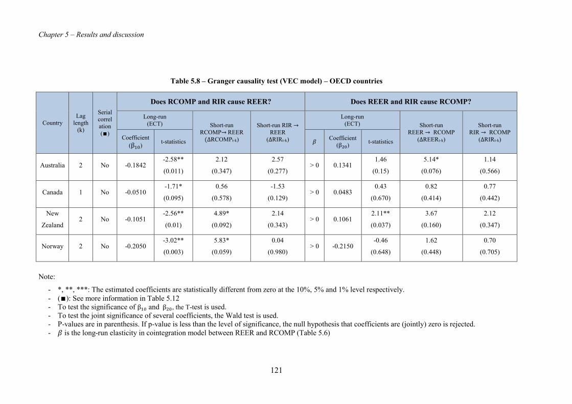
Chapter 5 – Results and discussion
121
Table 5.8 – Granger causality test (VEC model) – OECD countries
Country Lag
length (k)
Serial correlation (∎)
Does RCOMP and RIR cause REER? Does REER and RIR cause RCOMP?
Long-run (ECT) Short-run
RCOMP→ REER (∆RCOMPt-k)
Short-run RIR → REER
(∆RIRt-k)
Long-run (ECT) Short-run
REER → RCOMP (∆REERt-k)
Short-run RIR → RCOMP
(∆RIRt-k) Coefficient (β10) t-statistics 𝛽 Coefficient
(β20) t-statistics
Australia 2 No -0.1842 -2.58**
(0.011)
2.12
(0.347)
2.57
(0.277) > 0 0.1341
1.46
(0.15)
5.14*
(0.076)
1.14
(0.566)
Canada 1 No -0.0510 -1.71*
(0.095)
0.56
(0.578)
-1.53
(0.129) > 0 0.0483
0.43
(0.670)
0.82
(0.414)
0.77
(0.442)
New
Zealand 2 No -0.1051
-2.56**
(0.01)
4.89*
(0.092)
2.14
(0.343) > 0 0.1061
2.11**
(0.037)
3.67
(0.160)
2.12
(0.347)
Norway 2 No -0.2050 -3.02**
(0.003)
5.83*
(0.059)
0.04
(0.980) > 0 -0.2150
-0.46
(0.648)
1.62
(0.448)
0.70
(0.705)
Note:
- *, **, ***: The estimated coefficients are statistically different from zero at the 10%, 5% and 1% level respectively. - (∎): See more information in Table 5.12 - To test the significance of β10 and β20, the T-test is used. - To test the joint significance of several coefficients, the Wald test is used. - P-values are in parenthesis. If p-value is less than the level of significance, the null hypothesis that coefficients are (jointly) zero is rejected. - 𝛽 is the long-run elasticity in cointegration model between REER and RCOMP (Table 5.6)

Chapter 5 – Results and discussion
122
Table 5.9 – Granger causality test proposed by Toda and Yamamoto (VAR model) – OECD countries
Country Lag
length (k)
Maximum order of
integration (m)
Serial correlation
(∎)
Does RCOMP and RIR cause REER? Does REER and RIR cause RCOMP?
RCOMP→ REER (RCOMPt-k)
RIR→ REER (RIRt-k)
REER→ RCOMP (REERt-k)
RIR→ RCOMP (RIRt-k)
Iceland 1 1 No 0.17 (0.68)
0.45 (0.50)
1.48 (0.22)
0.05 (0.83)
Greece 4 1 No 0.17 (0.68)
0.45 (0.50)
1.48 (0.22)
0.05 (0.83)
Note:
- *, **, ***: The estimated coefficients are statistically different from zero at the 10%, 5% and 1% level respectively. - (∎): See more information in Table 5.13 - To test the joint significance of several coefficients, the Wald test is used. - P-values are in parenthesis. If p-value is less than the level of significance, the null hypothesis that coefficients are (jointly) zero is rejected.

Chapter 5 – Results and discussion
123
Table 5.10 – Granger causality test (VEC model) – ASEAN countries
Country Lag
length (k)
Serial correla
tion (∎)
Does RCOMP and RIR cause REER? Does REER and RIR cause RCOMP?
Long-run (ECT) Short-run
RCOMP→ REER (∆RCOMPt-k)
Short-run RIR → REER
(∆RIRt-k)
Long-run (ECT) Short-run
REER → RCOMP (∆REERt-k)
Short-run RIR → RCOMP
(∆RIRt-k) Coefficient (β10) t-statistics 𝛽 Coefficient
(β20) t-statistics
Brunei 1 No 0.0186 1.44 (0.15)
-0.44 (0.66)
-0.01*** (0.00) < 0 -0.5620 -2.57**
(0.01) -0.40 (0.69)
-1.90* (0.06)
Note:
- *, **, ***: The estimated coefficients are statistically different from zero at the 10%, 5% and 1% level respectively. - (∎): See more information in Table 5.12 - To test the significance of β10 and β20, the T-test is used. - To test the joint significance of several coefficients, the Wald test is used. - P-values are in parenthesis. If p-value is less than the level of significance, the null hypothesis that coefficients are (jointly) zero is rejected. - 𝛽 is the long-run elasticity in cointegration model between REER and RCOMP (Table 5.7)

Chapter 5 – Results and discussion
124
Table 5.11 – Granger causality test proposed by Toda and Yamamoto (VAR model) – ASEAN countries
Country Lag
length (k)
Maximum order of
integration (m)
Serial correlation
(∎)
Does RCOMP and RIR cause REER? Does REER and RIR cause RCOMP?
RCOMP→ REER (RCOMPt-k)
RIR→ REER (RIRt-k)
REER→ RCOMP (REERt-k)
RIR→ RCOMP (RIRt-k)
Laos 7 1 No 39.92*** (0.00)
47.40*** (0.00)
10.60 (0.16)
20.85*** (0.00)
Malaysia 1 1 No 0.04 (0.84)
0.28 (0.60)
0.05 (0.82)
0.21 (0.65)
Myanmar 7 1 No 7.51 (0.38)
17.53** (0.01)
3.34 (0.85)
5.48 (0.60)
Thailand 3 1 No 3.09 (0.37)
2.51 (0.47)
1.80 (0.62)
9.69** (0.02)
Vietnam 3 1 No 7.42* (0.06)
0.98 (0.80)
4.82 (0.19)
6.17* (0.10)
Note:
- *, **, ***: The estimated coefficients are statistically different from zero at the 10%, 5% and 1% level respectively. - (∎): See more information in Table 5.13 - To test the joint significance of several coefficients, the Wald test is used. - P-values are in parenthesis. If p-value is less than the level of significance, the null hypothesis that coefficients are (jointly) zero is rejected.

Chapter 5 – Results and discussion
125
Table 5.12 – Residual serial correlation Lagrange multiplier test for VEC models
Country LM statistics Conclusion
Australia 4.48 (0.35) No serial correlation
New Zealand 3.70 (0.45) No serial correlation
Norway 4.51 (0.34) No serial correlation
Brunei 1.47 (0.83) No serial correlation
Table 5.13 – Residual serial correlation Lagrange multiplier test for VAR models
Country LM statistics Conclusion
Canada 6.54 (0.69) No serial correlation
Iceland 13.29 (0.15) No serial correlation
Greece 8.63 (0.47) No serial correlation
Laos 5.91 (0.75) No serial correlation
Malaysia 11.36 (0.25) No serial correlation
Myanmar 9.36 (0.40) No serial correlation
Thailand 7.19 (0.62) No serial correlation
Vietnam 5.78 (0.76) No serial correlation
Note: P-value is in parenthesis

Chapter 5 – Results and discussion
126
RCOMP and RIR in level and first difference.
a. OECD
For individual OECD countries, the unit root test results on level and first difference of
the three variables REER, RCOMP and RIR are shown in Table 5.1.
The test results reveal that for six OECD countries, all variables REER, RCOMP and
RIR are integrated of order one (I(1)), except RIR for New Zealand. It can be said that
in each country the three variables are not stationary in level but stationary in first
difference. Only in New Zealand, RIR is stationary in level.
b. ASEAN
Table 5.2 summarizes the unit root test results on level and first difference of the
variables for individual ASEAN commodity-exporting countries.
For five ASEAN countries−Brunei, Laos, Malaysia, Myanmar and Thailand−the unit
root test results show that REER and RCOMP are found to be integrated of order one
(I(1)) while RIR is stationary I(0). The unit test results of Vietnam are quite different.
Only RCOMP is integrated of order one (I(1)) while REER and RIR are stationary in
level I(0).
5.1.1.2 Johansen (1988) cointegration test
Based on the unit root tests results, we cannot apply a Johansen (1988) cointegration
test for Vietnam, as this test requires the same order of integration of the two variables
REER and RCOMP.
For the eleven remaining countries where REER and RCOMP are both I(1), we use a
Johansen (1988) cointegration test to examine whether REER and RCOMP are
cointegrated. Table 5.4 and 5.5 provide the results of the Johansen (1988) cointegration
test for individual OECD and ASEAN commodity-exporting countries.
a. OECD
As mentioned in section 4.3.1.2, the lag length for a Johansen (1988) cointegration test
is one fewer than the lag length for a VAR model. The lag length for the Johansen
(1988) cointegration test of each country is shown in Table 5.3.

Chapter 5 – Results and discussion
127
Table 5.4 shows the results of Johansen (1988) cointegration tests between REER and
RCOMP in OECD countries. The results indicate that REER and RCOMP are
cointegrated in four out of six countries, including Australia, Canada, New Zealand, and
Norway.
Specifically, for Australia and Norway, the null hypothesis of no cointegration (r = 0),
is clearly rejected since both trace statistics and maximum eigenvalue statistics exceed
the critical values at the 10% significance level. However, the null hypothesis of no
more than one cointegrating equation (r ≤1) cannot be rejected at the 10% level. This
suggests that in Australia and Norway there is one cointegrating equation between
REER and RCOMP. For New Zealand, both the trace test and the maximum eigenvalue
test indicate two cointegrating relations between REER and RCOMP at 10%
significance level.
For Canada, the results of Johansen’s trace test and maximum eigenvalue test are
inconsistent. According to the trace test, the null hypothesis of no cointegration (r = 0)
cannot be rejected. Thus, there is no cointegrating equation between REER and
RCOMP. Meanwhile, the result of the maximum eigenvalue test implies one
cointegrating equation between the two variables. Because the maximum eigenvalue
test normally pins down the number of cointegrating vectors (Enders 2004), it can be
concluded that for Canada, there is one cointegrating equation between REER and
RCOMP .
The Johansen (1988) cointegration test fails to indicate long-run relationships between
REER and RCOMP in Iceland and Greece. Based on the acceptance of the null
hypothesis of no cointegrating equation (r = 0), both the trace test and maximum
eigenvalue test indicate no cointegration between the two variables. This implies that in
Iceland and Greece, REER and RCOMP appear to move independently and are not
bound together in the long run.
b. ASEAN
Brunei is the only country among ASEAN countries where REER and RCOMP are
cointegrated. As shown in Table 5.5, in both the trace test and maximum eigenvalue
test, the null hypothesis of no cointegration (r = 0) is rejected while the null hypothesis
of no more than one cointegrating equation (r = 1) cannot be rejected. It can be

Chapter 5 – Results and discussion
128
concluded that there is one cointegrating equation between REER and RCOMP. In
Laos, Malaysia, Myanmar and Thailand, both the trace test and maximum eigenvalue
test indicate that there is no cointegration between REER and RCOMP. Generally, in
most ASEAN commodity-exporting countries, there is no evidence of a long-run
relationship between REER and RCOMP, except for Brunei.
5.1.1.3 Cointegrating equations
For Australia, Canada, New Zealand, Norway and Brunei where REER and RCOMP
are cointegrated, cointegrating equations are estimated.
a. OECD
The cointegrating equations, when normalized for a unit coefficient on REER, of
Australia, Canada, New Zealand and Norway are illustrated in Table 5.6. The slope
coefficient β measures the long-run elasticity of REER with respect to RCOMP. β can
be translated as the percentage change in REER for a percentage change in RCOMP.
In Australia, the coefficient of RCOMP is statistically significant at 5% significance
level because the absolute t-statistic value (8.092) is larger than the critical value
(1.960). Moreover, the coefficient is positive, which suggests that REER and RCOMP
are positively related. When RCOMP increases by 1%, on average, REER increases by
about 0.38%.
In Canada and Norway, the coefficient of RCOMP is lower: 0.2127 and 0.0377,
respectively. The largest coefficient belongs to New Zealand, which is 0.7546. In New
Zealand, when RCOMP increases by 1%, REER goes up by approximately 0.75%.
In summary, the long-run coefficients of RCOMP are all statistically significant and
positive in OECD countries. This implies that RCOMP and REER move together in
long-run with the same direction (up or down together).
b. ASEAN
Among ASEAN commodity-exporting countries, Brunei is the only country where
exchange rate and commodity prices have a long-run relationship. As shown in Table
5.7, the coefficient of RCOMP ( β ) is statistically different from zero at the 5%
significance level. This can be concluded because t-statistic value (4.062) is larger than

Chapter 5 – Results and discussion
129
the critical value.
However, this coefficient is positive (0.2361). This suggests that in the long run,
RCOMP and REER move together in same direction. Specifically, if RCOMP increases
1%, REER increases 0.24% on average, and vice versa.
5.1.1.4 Granger causality tests
As mentioned in Section 4.3 – Research methodology, in case REER and RCOMP are
cointegrated, a VEC model will be used to test for Granger causality between the two
variables. Otherwise, Toda and Yamamoto (1995) augmented VAR model will be used
to test for Granger causality.
a. OECD
Australia, Canada, New Zealand and Norway:
According to the Johansen (1988) cointegration test, REER and RCOMP are found to
be cointegrated in Australia, Canada, New Zealand and Norway. Therefore, Granger
causality between REER and RCOMP will be investigated based on a VEC model
(Equations (4.15) and (4.16)). The test results for each country are reported in Table 5.8.
For Australia, the coefficient of ECT (β10) in Equation (4.15) is statistical significant at
the 5% significance level. Moreover, it is negative (−0.1842) and its absolute value is
less than one. It can be concluded that there is long-run Granger causality running from
RCOMP to REER. However, there is no evidence of Granger causality from REER to
RCOMP since the coefficient of ECT (β20 ) in Equation (4.16) is not significant.
Regarding short-run Granger causality,37 the significance of the first differences of
lagged REERs in Equation (4.16) indicates that there is a unidirectional short-run
Granger causality running from REER to RCOMP.
For Canada, RCOMP Granger-causes REER in the long run, but not vice versa. This
can be explained by noting that the coefficient of ECT (β10) in Equation (4.15) is
negative (−0.0510), statistically different from zero at the 10% significance level and
37 The term “Granger causality” always implies a short-term relationship (Gujarati 2009). The term “short-run Granger causality” is only used to easily distinguish “Granger causality” from “long-run Granger causality.”

Chapter 5 – Results and discussion
130
less than one in absolute value. There is no evidence of short-run Granger causality in
either direction.
For New Zealand, there is two-way long-run Granger causality between REER and
RCOMP since both coefficients of ECT in both equations (β10 and β20) are significant
at the 5% level and have appropriate sign and magnitude. Specifically, β10 (−0.1051) is
negative and its absolute value is less than one, and the sign of β20 (0.1061) satisfies the
requirement −β20.β < 0 (as β > 0). Based on the Wald test result, all the coefficients of
first-differenced lagged RCOMPs in Equation (4.15) are found to be jointly significant
while that of first-differenced lagged REERs in Equation (4.16) are not jointly
significant. This implies unidirectional short-run Granger causality running from REER
to RCOMP.
For Norway, the significance of ECT (β10 ) in Equation (4.15) at the 5% level of
significance suggests a long-run Granger causality from RCOMP to REER. In addition,
there is also Granger causality running from RCOMP to REER in the short-run since
the coefficients of lagged RCOMPs in Equation (4.15) are jointly statistically different
from zero at the 10% level of significance. There is no short-run or long-run Granger
causality in the opposite direction.
Iceland, Greece:
The Johansen (1988) cointegration test results for Iceland and Greece indicate that
REER and RCOMP are not cointegrated. Therefore, for Iceland and Greece, the
direction of the Granger causality will be detected through the Toda and Yamamoto
(1995) augmented VAR model (Equations (4.13) and (4.14)). Table 5.9 shows the
Granger causality test results for these two countries based on the augmented VAR
model.
For Iceland and Greece, the Wald test result reveals that both the coefficients related to
the lagged RCOMPs and the coefficients related to REERs are not jointly significant.
This indicates no Granger causality between REER and RCOMP.
In short, there is long-run Granger causality running from RCOMP to REER in four out
of six OECD commodity-exporting countries: Australia, Canada, New Zealand, and
Iceland. Regarding short-run Granger causality, while in New Zealand and Norway
Chapter 5 – Results and discussion
131
RCOMP Granger-causes REER, in Australia, REER leads RCOMP in the short-run and
there is no short-run Granger causality in Canada. Moreover, there is no evidence of
Granger causality from RIR to either RCOMP or REER. It is also worth noting that
there is no serial correlation in both VEC and VAR models (see Table 5.12 and 5.13).
b. ASEAN
Brunei
Because REER and RCOMP are found to be cointegrated in Brunei, Granger causality
between REER and RCOMP is therefore investigated based on a VEC model. It can be
seen from Table 5.10 that the estimated coefficient of ECT (β20) in Equation (4.16) is
statistically significant at the 5% level of significance with appropriate sign (– β20.β <
0). In particular, both β20 ( − 0.5620) and β ( − 0.2361) are negative so – β20 . β is
negative as expected. Meanwhile, β10 is not statistically significant. This suggests that
there is a long-run Granger causality running from REER to RCOMP. In addition, there
is no evidence of short-run Granger causality between REER and RCOMP. It is
interesting to note that RIR Granger causes both RCOMP and REER in the short-run.
Laos, Malaysia, Myanmar, Thailand and Vietnam:
For the five remaining developing countries−Laos, Malaysia, Myanmar, Thailand and
Vietnam − where REER and RCOMP are not cointegrated, we utilize Toda and
Yamamoto (1995) augmented VAR model to explore the Granger causality between the
variables. Table 5.11 shows the Wald test results for the joint significance of lagged
independent variables.
For Laos, based on the joint significance of lagged RCOMPs, it can be concluded that,
in these two countries, there is Granger causality running from RCOMP to REER.
There is no evidence of Granger causality in the opposite direction.
Similar to Laos, Vietnam has a short-run unidirectional Granger causality with the
direction from RCOMP to REER. For Malaysia, Myanmar and Thailand, no Granger of
causality between REER and RCOMP can be found.
In short, among six ASEAN commodity-exporting countries, long-run Granger
causality between REER and RCOMP can only be found in Brunei with the direction

Chapter 5 – Results and discussion
132
from RCOMP to REER. Three out of the five remaining countries, namely Malaysia,
Myanmar, and Thailand, show no Granger causality relationship between RCOMP and
REER. In Vietnam and Laos, there is short-run Granger causality from RCOMP to
REER.
It is worth mentioning that short-run Granger causality implies only the short-term
relationship between variables while theory as well as policy implications typically have
not much to say about short-term relationships (Thomas 1993). Because one of our
main purposes is providing policy implications for ASEAN commodity-exporting
countries in their transition period to become developed countries, the long-run Granger
causality is our main concern.
While in OECD countries, there is no evidence of Granger causality from RIR to either
RCOMP or REER; RIR seems to have more influence on REER and RCOMP in
ASEAN. Specifically, in Brunei and Laos, RIR Granger-causes both RCOMP and
REER. In Vietnam and Thailand, Granger causality is running from RIR to RCOMP,
while in Myanmar, Granger causality runs from RIR to REER. The only country where
there is no Granger causality from RIR to either RCOMP or REER is Malaysia.
5.1.2 Groups of countries
The panel-data technique is applied for each group – OECD commodity-exporting
countries group and ASEAN commodity-exporting countries – to investigate the most
common characteristics of the relationship between REER and RCOMP in each group.
5.1.2.1 Panel unit root tests
The panel unit root tests are applied both in level and first difference for all variables
REER, RCOMP, and RIR. Table 5.14 shows the panel unit root test results for each
group, OECD and ASEAN.
a. OECD
According to the three panel unit root tests including – Im, Pesaran and Shin (2003),
Maddala and Wu (1999) and Choi (2001) – we cannot reject the null hypothesis of unit
root when the three variables are taken in level. Nevertheless, when the first-difference
is used, the null hypothesis can be rejected at the 1% level of significance. Therefore,
Chapter 5 – Results and discussion
133
we can conclude that in OECD commodity-exporting countries, all variables – REER,
RCOMP and RIR – are integrated of order one (I(1)).
b. ASEAN
For the ASEAN group, the panel unit test results indicate that REER and RCOMP are
both integrated of order one (I(1)). As shown in Table 5.14, all the three panel unit root
tests (both with and without trend) reveal that REER and RCOMP are not stationary in
level but stationary in first difference.
Meanwhile, all of the panel unit root test results show that RIR is stationary in level
(I(0)).

Chapter 5 – Results and discussion
134
Table 5.14 – Panel unit root tests for REER, RCOMP and RIR
Group Variables Level/ First
difference
Im Pesaran and Shin Test Statistic
Maddala and Wu Test Statistic
Choi Test statistic
Conclusion Without
trend With trend
Without trend
With trend
Without trend
Without trend
6 OECD
countries
REER Level
1st difference
-1.21 (0-2)
-24.96 (0-1)*
-0.74 (0-3)
-25.61 (0-1)*
16.55 (0-2)
379.75 (0-1)*
15.07 (0-3)
348.67 (0-1)*
18.49
389.60*
12.97
358.30* I(1)
RCOMP Level
1st difference
-0.70 (0-1)
-20.99 (0-1)*
-0.23 (0-1)
-20.66 (0-1)*
14.00 (0-1)
316.11 (0-1)*
10.53 (0-1)
277.92 (0-1)*
10.44
330.53*
6.93
305.36* I(1)
RIR Level
1st difference
-1.20 (0-8)
-25.48 (0-6)*
-3.86 (0-8)
-26.22 (0-6)*
20.81 (0-8)
348.50 (0-6)*
51.31 (0-8)*
318.06 (0-6)*
16.79
353.13*
82.03*
316.609* I(1)
6 ASEAN
countries
REER Level
1st difference
-1.04 (0-10)
-17.36 (0-5)*
2.15 (0-10)
-17.88 (0-9)*
16.35 (0-10)
191.38 (0-5)*
8.98 (0-10)
220.73 (0-9)*
25.60*
240.07*
13.35
306.23* I(1)
RCOMP Level
1st difference
-0.22 (0-2)
-17.80 (0-1)*
-0.64 (0-2)
-17.63 (0-1)*
9.43 (0-2)
245.84 (0-1)*
14.33 (0-2)
225.50 (0-1)*
8.75
273.07*
11.19
264.43* I(1)
RIR Level
1st difference
-3.78 (2-11)*
-10.65 (2-11)*
-5.55 (0-12)*
-9.68 (2-11)*
42.99 (2-11)*
143.54 (2-11)*
51.61 (0-12)*
120.16 (2-11)*
92.89*
304.73*
91.99*
350.75* I(0)
Note:
- Lag length is in parenthesis, which is chosen following Akaike Info Criterion. - For Choi (2001) unit root test, Newey-West automatic bandwidth selection and Bartlett kernel is selected. - * denotes that the null hypothesis of unit root is rejected at 5% significance level or series is stationary.

Chapter 5 – Results and discussion
135
Table 5.15 – Pedroni (1999) Panel Cointegration Test for REER and RCOMP – 6 OECD countries
Statistics Individual intercept Individual intercept
and trend
Panel statistics
Variance ratio statistic 2.29* 2.26*
Rho statistic -2.13* -3.71*
PP statistic -1.82* -3.06*
ADF statistic -1.66* -3.54*
Group statistics
Rho statistic -2.02* -3.16*
PP statistic -2.03* -3.06*
ADF statistic -1.66* -3.21*
Cointegration Yes Yes
CONCLUSION REER and RCOMP are cointegrated
Notes: * implies that the null of no cointegration is rejected at the 5% level of significance.

Chapter 5 – Results and discussion
136
Table 5.16 – Pedroni (1999) Panel Cointegration Test for REER and RCOMP – 6 ASEAN countries
Statistics Individual intercept Individual intercept
and trend
Panel statistics
Variance ratio statistic -2.22 4.72*
Rho statistic 1.54 -0.46
PP statistic 0.47 0.18
ADF statistic 0.74 -0.32
Group statistics
Rho statistic -0.68 -2.60*
PP statistic -1.48 -2.64*
ADF statistic -0.02 -1.05
Cointegration No No
CONCLUSION REER and RCOMP are not cointegrated
Notes: * implies that the null of no cointegration is rejected at the 5% level of significance.

Chapter 5 – Results and discussion
137
Table 5.17 – Granger causality test (panel VEC model) – 6 OECD countries
Group Lag
length (k)
Serial correlation
(∎)
Does RCOMP and RIR cause REER? Does REER and RIR cause RCOMP? Long-run
(ECT) Short-run RCOMP→ REER
(∆RCOMPt-k)
Short-run RIR → REER
(∆RIRt-k)
Long-run (ECT) Short-run
REER → RCOMP (∆REERt-k)
Short-run RIR → RCOMP
(∆RIRt-k) Coefficient (β10) t-statistics 𝛽 Coefficient
(β20) t-statistics
6 OECD
countries 5 No -0.05
-3.56***
(0.00)
8.47
(0.13)
7.55
(0.18) > 0 0.05
1.26
(0.21)
18.30***
(0.00)
7.90
(0.16)
Note:
- *, **, ***: The coefficients are statistically significant at the 10%, 5% and 1% level respectively. - (∎): See more information in Table 5.18 - To test the significance of β10 and β20, the T-test is used. - To test the joint significance of several coefficients, the Wald test is used. - P-values are in parenthesis. If p-value is less than the level of significance, the null hypothesis that coefficients are (jointly) zero is rejected. - 𝛽 is the long-run elasticity in cointegration model between REER and RCOMP (Equation (5.1))
Table 5.18 – Residual serial correlation Lagrange multiplier (LM) test for panel VEC model
Note: P-value is in parenthesis
Lag length LM statistics Conclusion
5 6.90
(0.14) No serial correlation

Chapter 5 – Results and discussion
138
Table 5.19 – Granger causality test proposed by Toda and Yamamoto (VAR model) – 6 ASEAN countries
Group Lag length (k)
Maximum order of
integration (m)
Serial correlation
(∎)
Does RCOMP and RIR cause REER? Does REER and RIR cause RCOMP?
Short-run RCOMP→ REER (RCOMPt-k)
Short-run RIR→ REER (RIRt-k)
Short-run REER→RCOMP
(REERt-k)
Short-run RIR→RCOMP (RIRt-k)
6 ASEAN
countries 5 1 No
3.93
(0.69)
8.66
(0.19)
5.05
(0.54)
2.55
(0.86)
Note:
- *, **, ***: The coefficients are statistically significant at the 10%, 5% and 1% level respectively. - (∎): See more information in Table 5.20 - To test the joint significance of several coefficients, the Wald test is used. - P-values are in parenthesis. If p-value is less than the level of significance, the null hypothesis that coefficients are (jointly) zero is rejected.
Table 5.20 – Residual serial correlation Lagrange multiplier test for VAR model
Lag length LM statistics Conclusion
6 28.07
(0.00) Serial correlation
5 4.53
(0.87) No serial correlation
Note: P-value is in parenthesis

Chapter 5 – Results and discussion
139
5.1.2.2 Pedroni (1999) panel cointegration tests
The results of the panel unit root tests show that in OECD and ASEAN, REER and
RCOMP are cointegrated of same order (both of them are I(1)). This enables us to test
for the cointegration between REER and RCOMP for the two groups. As mentioned in
Section 4.3.2.2, to examine whether a cointegrating relationship exists between REER
and RCOMP, we employ the Pedroni (1999) panel cointegration test.
a. OECD
The Pedroni (1999) panel cointegration test results for OECD are shown in Table 5.15.
A Pedroni (1999) panel cointegration test is applied with individual intercept only or
with both individual intercept and trend. In both cases, all seven tests can reject the null
hypothesis of no cointegration at the significance level of 5%. It can be concluded that
REER and RCOMP are cointegrated.
The cointegrating equation (following Equation (4.23)) between REER and RCOMP is
estimated by group-mean DOLS as follows:
REER = 3.3488 + 0.2782 RCOMP (5.1) (0.104) [-2.689] Note: Standard errors in ( ) and t-statistics in [ ]
The long-run elasticity of REER in response to RCOMP is 0.2782. This implies that
REER and RCOMP move together in the long run with the same direction. For
example, if RCOMP increases 1%, REER increases nearly 0.28% on average.
b. ASEAN
As presented in Table 5.16, in both cases – with and without trend – the Pedroni (1999)
panel cointegration results show that there is no cointegration between REER and
RCOMP for ASEAN.
Specifically, in the case of intercept only, all of the seven tests cannot reject the null
hypothesis of no cointegration at the 5% significance level. For this case, it is quite clear
that REER and RCOMP are not cointegrated.
In the case of both intercept and trend, the majority of tests (four out of seven tests
namely panel Rho statistic, panel PP statistic, panel ADF statistic, group ADF statistic)
cannot reject the null hypothesis of no cointegration at the 5% significance level. As the

Chapter 5 – Results and discussion
140
majority of tests show no cointegration between REER and RCOMP, it can be
concluded that REER and RCOMP are not cointegrated.
5.1.2.3 Panel Granger causality tests
It can be inferred from the Pedroni (1999) panel cointegration results that in OECD,
REER and RCOMP are cointegrated. Therefore, we use the VEC model to examine the
Granger causality between REER and RCOMP. For ASEAN, Toda and Yamamoto
(1995) augmented VAR model will be employed when testing for Granger causality.
a. OECD
As depicted in Table 5.17, the coefficient of ECT (β10) in Equation (4.26) is statistically
significant at the 1% level of significance. Moreover, β10 (−0.05) has a proper sign
(negative) and is less than one in absolute value. Thus, it can be stated that in the long
run, RCOMP Granger-causes REER. Since the coefficient of ECT (β20) in Equation
(4.27) is not statistically significant, there is no long-run Granger causality running from
REER to RCOMP.
Short-run Granger causality is detected based on Wald statistics test results. The Wald
statistics test proves that there is joint significance of first-differenced lagged REERs in
Equation (4.27) and no joint significance for other first-differenced lagged explanatory
variables. This implies that there is a unidirectional short-run causality running from
REER to RCOMP. In addition, RIR does not Granger-cause either REER or RCOMP.
b. ASEAN
Based on lag length selection criteria, the optimal lag length is 6. However, this lag
length leads to serial correlation in the VAR model (see Table 5.20). To avoid the serial
correlation, the lag length has been reduced to 5.
According to the results reported in Table 5.19, the Wald statistics test result based on
Equation (4.24) shows that the coefficients of first-differenced lagged RCOMPs are
jointly insignificant. In addition, the coefficients of first-differenced lagged REERs in
Equation (4.25) are also jointly insignificant at the 10% level of significance. We can
conclude that there are no Granger causality between REER and RCOMP in ASEAN.
Moreover, the Wald statistics test results also show that there is no Granger causality
running from RIR to either REER or RCOMP.

Chapter 5 – Results and discussion
141
5.2 Analysis of test results
In this part, the test results from both time-series and panel-data methods will be
analysed to provide insight into the relationship between exchange rate and commodity
prices in OECD and ASEAN.
5.2.1 OECD
For both OECD and ASEAN, the findings obtained from time-series and panel-data
techniques are relatively consistent.
Regarding cointegration, when applying the Johansen (1988) cointegration test for each
OECD commodity-exporting country, the test results indicate that in most OECD
countries (four out of six countries including Australia, Canada, New Zealand and
Norway), there is cointegration between real exchange rate and real commodity prices.
These findings are consistent with what is being implied by the panel cointegration test
result. The Pedroni (1999) panel cointegration test on the group of six OECD countries
also finds out that real exchange rate and real commodity prices move together in the
long-run.
While estimating cointegrating equations for individual countries (Australia, Canada,
New Zealand and Norway), all the coefficients of real commodity prices in
cointegrating equations are positive. The estimation result by the DOLS method for the
OECD panel data set shows the same result. This implies that in OECD commodity-
exporting countries, real exchange rate and real commodity prices move together in the
long-term with the same direction.
About Granger causality, both time-series and panel-data methods indicate that there is
long-run Granger causality running from commodity prices to exchange rate in OECD
commodity-exporting countries. Specifically, the result of the Granger causality test
applied for OECD panel data set implies that there is evidence of unidirectional Granger
causality from commodity prices to exchanger rate in OECD countries. In line with this
finding, following the Granger test results for individual countries, in four out of six
OECD countries, which are Australia, Canada, New Zealand and Norway, commodity
prices Granger-causes exchange rate in the long-run. It can be concluded that in OECD
commodity-exporting countries, real commodity prices are initial receptors of

Chapter 5 – Results and discussion
142
exogenous shocks to the long-run equilibrium and real exchange rate always responses
to changes in real commodity prices in order to maintain the long-run relationship
between the two variables. This finding is in line with some existing works Simpson
and Evans (2004), Trezzi (2014), Harri, Nalley and Hudson (2009) and Chaudhuri and
Daniel (1998)).
Whereas the two empirical methods provide consistent findings about long-run Granger
causality, the findings about short-run Granger causality are somewhat contradictory.
According to Granger causality test results for individual countries: in Australia, real
exchange rate Granger-causes real commodity prices in the short run; in New Zealand
and Norway, Granger causality runs in the opposite direction, from real commodity
prices to real exchange rate; and in the three remaining countries of Canada, Iceland and
Greece, there is no short-run Granger causality in either direction. On the other hand,
the results of Granger causality tests performed on OECD panel data set indicate an
existence of short-run Granger causality running from real exchange rate to real
commodity prices in OECD commodity-exporting countries.
5.2.2 ASEAN
The test results from both time-series and panel-data techniques show that the
relationship between exchange rate and commodity prices in ASEAN commodity-
exporting countries is considerably different from that in OECD commodity-exporting
countries.
In regard to cointegration, in most of the ASEAN commodity-exporting countries (five
out of six) there is no evidence of cointegration between real exchange rate and real
commodity prices. Only in Brunei – the largest oil exporter in ASEAN – real exchange
rate and real commodity prices are cointegrated. Moreover, the result of panel
cointegration tests on the group of six ASEAN countries also indicates that there is
cointegration between these two variables. Therefore, it can be concluded that in
ASEAN commodity-exporting countries, real exchange rate and real commodity prices
move independently in the long run.
Because of the lack of cointegration between real exchange rate and real commodity
prices, there is obviously no long-run Granger causality between these two variables in

Chapter 5 – Results and discussion
143
ASEAN countries. Based on panel Granger causality test results, there is also no
evidence of short-run Granger causality between real exchange rate and real commodity
prices. This finding is consistent with the finding from time-series techniques that only
two out of six ASEAN countries (Vietnam and Laos) have short-run Granger causality
running from real commodity prices to real exchange rate.
On the whole, there is a significant difference in the relationship between exchange rate
and commodity prices in ASEAN and OECD commodity-exporting countries. While
exchange rate and commodity prices have a long-term relationship in OECD, there is no
long-run or short-run relationship between the two variables in ASEAN countries. In
other words, the commodity prices – exchange rate nexus in ASEAN countries is not
obvious.
5.3 Discussion
It can be derived from the test results that most OECD commodity-exporting countries
have a strong relationship between real exchange rate and real commodity prices.
Specifically, changes in real commodity prices will lead to responses of real exchange
rate to re-establish the equilibrium in the long run. This finding is in line with Cashin,
Céspedes and Sahay (2004) theory (mentioned in Section 1.4).
However, in ASEAN commodity exporting countries, the relationship between real
commodity prices and real exchange rate is not obvious. The difference in the
commodity prices – exchange rate nexus between OECD and ASEAN can be explained
as follows.
Different exchange rate regimes
OECD countries adopt a free-floating exchange rate while ASEAN countries manage
their exchange rate or peg their currencies to a major currency or to a basket of
currencies. In fact, Australia, Canada, New Zealand, and Norway adopted a free-
floating exchange rate regime quite early. Canada was the first Western country to
move to a floating exchange rate (in 1970) after the Second World War. Australia and
New Zealand in turn decided to float the exchange rate in 1983 and 1985, respectively.
For Norway, after fixing the exchange rate from 1986 to the end of the decade, in 1992,
the country decided to float the Norwegian krone after the demand shock caused by the

Chapter 5 – Results and discussion
144
reunification of the Germany. Iceland and Greece are two countries that adopted a free-
floating exchange rate so late. Iceland had pegged the value of the Króna to a basket of
nine currencies until 2000 and decided to float the Króna in 2001. Greece also began
floating its exchange rate in 2001. Before that, the exchange rate for the drachma is
determined in the domestic and foreign interbank markets, as well as in daily fixing
sessions in which the Bank of Greece (BOG) and authorized commercial banks
participate.
Meanwhile, ASEAN commodity-exporting countries have been in favour of a managed
floating and pegged exchange rate regime through the period from 1986 to 2014. As can
be seen from Table 5.21, there is a trend to move from pegged exchange rate regime to
managed floating regime in ASEAN countries, except for Brunei. From 1984 to now,
Brunei has maintained a currency board arrangement and tied its currency to the
Singapore dollar. This regime eliminates traditional central bank functions of the Brunei
Currency Board such as lender of last resort and monetary control. In Laos, Malaysia,
and Thailand, before adopting a managed floating exchange rate, the currencies of these
countries had been pegged against the USD for a long time. Specifically, from 1953 to
1988, the Lao kip was fixed to the USD. After that, Laos adopted a managed floating
system. Malaysia adopted a pegged arrangement system exchange rate from 1975,
pegging against the USD at MYR 3.80 per 1 USD. Since July 2005, this country has
adopted a managed floating system. Thailand is the only country in ASEAN that
announced the allowance of a free-floating exchange rate regime in July 1997, after 13
years of pegging to the USD at an exchange rate of around Baht 25 per 1 USD.
However, according to the IMF, Thailand fails to adapt requirements for a free-floating
exchange rate regime as the authorities of this country have indirectly intervened in the
foreign exchange market. This explains why the IMF reclassified the exchange rate
regime of Thailand as managed floating. Similarly, in Myanmar, the Myanmar kyat is
officially pegged to the SDR (Special Drawing Right) at Kyat 8.50847 per 1 SDR 30
years before becoming managed floating currency in June 2001 (as the result of the
liberalization of the secondary market for foreign exchange). In Vietnam, The State
Bank of Vietnam has managed its floating exchange rate most of the time by quoting an
interbank market rate as the daily average exchange rate in the interbank market during
the previous business day and setting up the range by which the participating banks can
quote rates.

Chapter 5 – Results and discussion
145
Table 5.21 – Exchange rate regimes
1986
1987
1988
1989
1990
1991
1992
1993
1994
1995
1996
1997
1998
1999
2000
2001
2002
2003
2004
2005
2006
2007
2008
2009
2010
2011
2012
2013
20 14
Australia F F M F F F F F
F
F F
F
F F F F F F F F F F F F F F F F F F F
Canada F F F F F F F F F F F F F F F F F F F F F F F F F F F F F
Iceland M M M PB PB PB PB PB PB PB PB PB PB PB PB F F F F F F F F M F M M M M
New Zealand F F F F F F F F F F F F F F F F F F F F F F F F F F F M M
Norway PB PB PB PB PB PB F F F F F F F F M M F F F F F F F F F F F F F
Greece M M M C C C M M M M M M M M M F F F F F F F F F F F F F F
Brunei C C C C C C C C C C C C C C C C C C C C C C C C C C C C C
Laos PU PU PU M M M M M M M M M M M M M M M M M M M M O S
A
S
A
S
A
S
A
Cr
Malaysia PU PU PU PU PU PU PU PU PU PU PU PU PU PU PU PU M PU PU M M M M M M M M M M
Myanmar PS PS PS PS PS PS PS PS PS PS PS PS PS PS PS PS PS PS PS PS PS PS PS PS PS PS M M M
Thailand PU PU PU PU PU PU PU PU PU PU PU M
(
M
)
M
(
M
)
M
(
M
)
M
(
M
)
M
(
M))
M M M M M M M M M M M M M
Vietnam PU PU M M M M M M M M M M M M M M M M M M M M M M
F
S
A
S
A
S
A
S
A
S Note: Source: Annual report on exchange arrangements and exchange restrictions
S: Stabilized arrangement M: Managed floating Cr: Crawling peg
C: Currency board F: Free-floating O: Other managed arrangement
PB: Pegged to a basket of currencies Ps: Pegged to SDR PU: Pegged to USD

Chapter 5 – Results and discussion
146
For a free-floating exchange rate regime, the exchange rate is determined by the market
forces and the monetary authority usually does not intervene in the foreign exchange
market. The intervention is only aimed at preventing excessive fluctuations in the
exchange rate (IMF 2007). Thus, it might enable the translation from real commodity
prices fluctuation to real exchange rate (according to Cashin, Céspedes and Sahay
(2004) theory). It can be said that the relationship between real exchange rate and real
commodity prices in OECD commodity-exporting countries is strong because most of
them freely float their exchange rate.
Meanwhile, ASEAN countries either manage their exchange rate or peg their currencies
to a major currency or to a basket of currencies. In a managed floating exchange rate
regime, the monetary authorities effect the movements of the exchange rate by
intervening actively in the foreign exchange market in order to maintain stability and
competitiveness of exchange rate. This intervention might lead the exchange rate to
deviate from its own way, preventing commodity prices and exchange from moving
together. Besides, in a pegged exchange rate regime, a currency will be pegged at a
fixed rate to another prevalent currency or a basket of currencies, by which a currency
will become more stable (IMF 2007). However in doing so, the pegged currency is then
controlled by its reference value (or the value of anchor currency). As such, the
movements of the exchange rate will be mainly dependent on the movement of
reference value, and not influenced by commodity prices. As a result, a pegged
exchange rate regime also contributes to weaken the relation between real exchange rate
and real commodity prices. It can be concluded that the use of both pegged and
managed floating exchange rate makes the relationship between real exchange rate and
real commodity prices in ASEAN countries rather obscured.
Based on the discussion above, we can conclude that late adoption of a free-floating
exchange rate is one of the reasons explaining why in Iceland and Greece real exchange
rate and real commodity prices do not have a long-run relationship.
Difference in ability to expand natural-resource sector
According to the “Dutch Disease” theory, in resource-rich countries, an increase in
natural resources commodity prices will make a given nation’s real exchange rate
appreciate (Brahmbhatt, Canuto & Vostroknutova 2010). To explain the “Dutch

Chapter 5 – Results and discussion
147
Disease” theory, researchers divide the economy into three sectors: the natural-resource
sector, the non-resource tradables sector (as agriculture and manufacturing), and the
nontradables sector. Natural resource commodity prices might affect real exchange rate
through two channels (Brahmbhatt, Canuto & Vostroknutova 2010). The first one is
spending effect. When commodity prices increase, export income will increase. This
normally leads to higher spending by public as well as private sectors. Consequently,
the demand for nontradables will increase. As the result, prices of nontradables will be
higher. On the other hand, wages in the economy will tend to rise. The increase in
wages will contribute to a rise in the relative prices of nontradables. As real exchange
rate is defined as the price of nontradables relative to the price of tradables, an increase
in commodity prices will lead to appreciation of real exchange rate. The second channel
is movement effect. A boom in the natural-resource sector will attract capital and labor
from the nontradables sector. It tends to reduce the output in the nontradables sector of
the economy. In particular, the output of the nontradables sector declines. This decline
makes the price of nontradables rise relative to the price of tradables (being set in the
world market), or real exchange rate appreciate. Through these two above channels, an
increase in commodity prices will lead to appreciation in real exchange rate.
However, the movement effect is less likely in ASEAN countries. This might be the
reason why the relationship between exchange rate and commodity prices is not obvious
in ASEAN. A lesser movement effect in ASEAN compared to OECD is clarified as
follows.
Natural resources such as crude oil, natural gas, minerals and woods dominate the
export of both ASEAN and OECD commodity-exporting countries. In fact, the
extraction of natural resources is very capital- and technology-intensive, especially
crude oil, natural gas, coal, and minerals. While OECD countries can run their own
natural resources extraction industry, ASEAN developing countries are strongly
dependent on FDI to develop their extractive industry because of the shortage of capital,
advanced technology and high-skilled labors (IESR 2014), (Sovacool 2010), and (Diana
& Maia 2000).

Chapter 5 – Results and discussion
148
In developing countries, the government tightly controls the extraction of natural
resources. State-owned national companies are major players in the natural-resource
sector, especially in oil extraction (Ross 2013; Pirog 2007). A limited source of finance
and lack of high technology prevent these state-owned national companies to expand
their operations. Thus, the most efficient way to develop the extractive industries in
ASEAN countries is to seek inflows of FDI (IESR 2014).
Nevertheless, the ability to attract FDI in the extractive industries in ASEAN is limited.
This can be explained by the fact that investing in extractive industries is normally more
risky than other sectors (Ruta & Venables 2012). Apart from the capital-intensive and
long-term nature of the mining industry, in the event of the project failing, a mine or oil
well cannot be dismantled and moved to another location (Ruta & Venables 2012).
Moreover, much of the crude oil and natural gas of Southeast Asia region is located in
deep-water offshore areas and a long way from the centre of demand; and much of the
mineral reserves is located in isolated areas which often lack basic services and
infrastructure, such as power. These things make investors ask for higher returns
(ASEAN 2014b).
Another main impediment to FDI across ASEAN countries is weak governance at many
levels, including an absence of rule of law, a lack of robust mechanisms to ensure
transparency and accountability to facilitate partnership between government and non-
government organizations, and lack of coordination among government agencies (IESR
2014; Ponciano, Narjoko & Simorangkir 2011). Moreover, the process for obtaining
exploration and mining licenses, or the resolution of land access issues, represents a
major impediment to investment in many ASEAN countries (IESR 2014). Apart from
Malaysia, the speed of processing in other developing ASEAN countries is classified as
slow and mainly slow (Ponciano, Narjoko & Simorangkir 2011). It is also worth
mentioning that some countries have their own problems that delay investment
decision-making of foreigners, such as political instability in Thailand, low investment
incentives and unstable macro economy in Vietnam, and high labor cost in Myanmar
(Ponciano, Narjoko & Simorangkir 2011). These factors, combined with the volatile
nature of commodity prices and high risks associated with extractive industry activities
prevent FDI in natural-resource sector in ASEAN countries.

Chapter 5 – Results and discussion
149
In summary, the expansion of the natural-resource sector in ASEAN countries mostly
relies on FDI. Meanwhile, investment attraction is not effective in these countries. Thus,
it can be said that the expansion or increasing productivity of the natural-resource sector
in the short term seems to be impossible. As mentioned above, the natural-resource
sector dominates the tradables sectors in commodity-exporting countries. Because of the
difficulty in expanding the operations of the natural-resource sector in ASEAN, the
movement of capital and labor from the nontradables sector to the natural-resource
sector (main tradables sector) in commodity booms is less likely to occur. For this
reason, the fluctuations in commodity prices are less likely to translate into volatility in
the real exchange rate in ASEAN countries than in OECD countries.
Difference in degree of financial openness
It is easily recognized that OECD countries have maintained much higher levels of
financial openness than ASEAN countries through the period from 1986 to 2014 (see
Table 5.22).
The degree of financial openness is measured using the KAOPEN index (Chinn & Ito
2006). As can be seen from Table 5.22, the level of financial openness is high in OECD
commodity-exporting countries (except for Iceland). Especially, Canada, New Zealand,
Norway and Greece are the most financially open in the world, with KAOPEN values of
2.42 for a long period (Chinn & Ito 2014). For Iceland, before 2008, this country
maintained a relatively high level of financial openness, with KAOPEN index of 1.11.
In 2008, there was a financial crisis in Iceland. Almost 90% of Iceland’s banking sector
failed in October (Iceland 2013a). This systemic banking collapse was the largest
experienced by any country in economic history. The crisis led to a low level of
financial openness afterwards (KAOPEN was negative, −1.18, from 2008 to 2012).
On the contrary, ASEAN commodity-exporting countries are not very financially open.
Specifically, KAOPEN indices of these countries are negative. Myanmar is the least
financially open with KAOPEN index of −1.88 most of the time.
According to Bodart, Candelon and Carpantier (2011), the response of the real
exchange rate to a commodity price shock will be more pronounced in more financially
open economies. They show that if capital is not mobile internationally, interest rate is
no longer exogenously given by the world interest rate but is determined endogenously

Chapter 5 – Results and discussion
150
Table 5.22 – KAOPEN index
Country 1995 1996 1997 1998 1999 2000 2001 2002 2003 2004 2005 2006 2007 2008 2009 2010 2011 2012
Australia 2.42 2.16 1.90 1.64 1.37 1.11 1.11 1.11 1.11 1.11 1.11 1.11 1.11 1.11 1.11 1.11 1.11 1.37
Canada 2.42 2.42 2.42 2.42 2.42 2.42 2.42 2.42 2.42 2.42 2.42 2.42 2.42 2.42 2.42 2.42 2.42 2.42
Iceland 1.11 1.11 1.11 1.11 1.11 1.11 1.11 1.11 1.11 1.11 1.11 1.11 1.11 -1.18 -1.18 -1.18 -1.18 -1.18
New Zealand 2.42 2.42 2.42 2.42 2.42 2.42 2.42 2.42 2.42 2.42 2.42 2.42 2.42 2.42 2.42 2.42 2.42 2.42
Norway 1.37 1.64 1.90 2.16 2.42 2.42 2.42 2.42 2.42 2.42 2.42 2.42 2.42 2.42 2.42 2.42 2.42 2.42
Greece -0.12 0.32 0.58 0.84 1.10 1.36 1.36 2.42 2.42 2.42 2.42 2.42 2.42 2.42 2.42 2.42 2.42 2.42
Laos -1.18 -0.12 -0.82 -0.82 -0.82 -0.82 -0.82 -0.82 -1.18 -1.18 -1.18 -1.18 -1.18 -1.18 -1.18 -1.18 -1.18 -1.18
Malaysia 1.19 0.93 0.67 0.41 0.14 -0.12 -0.12 -0.12 -0.12 -0.12 -0.12 -0.12 -0.12 1.11 -0.12 -1.18 -1.18 -1.18
Myanmar -1.18 -1.88 -1.88 -1.88 -1.88 -1.88 -1.88 -1.88 -1.88 -1.88 -1.88 -1.88 -1.88 -1.88 -1.88 -1.88 -1.88 -1.88
Thailand -0.12 -0.12 -0.12 -0.12 -0.12 -0.12 -0.12 -0.12 -0.12 -0.12 -0.12 -0.12 -1.18 -0.12 -1.18 -1.18 -1.18 -1.18
Vietnam -1.18 -0.91 -0.91 -0.91 -0.91 -0.91 -1.18 -1.18 -1.18 -1.18 -1.18 -1.18 -1.18 -0.12 -0.12 -0.12 -0.12 -0.12
Note: KAOPEN index is a measure of degree of financial openness. The data for Brunei is not available. Source: (Chinn & Ito 2008)

Chapter 5 – Results and discussion
151
from domestic conditions. It therefore appears that in response to a change in
commodity prices, exchange rate will remain unchanged because the marginal
productivity of capital and labor in the tradable sector is therefore fixed. This implies
that any increase in the export prices will lead to a proportional increase in the domestic
interest rate and the wage rate. In turn, the price of nontradables increases in the same
proportion, so leaving the real exchange rate unchanged. Thus, the relationship between
real exchange rate and commodity prices in ASEAN countries is not as strong as the
relationship in OECD countries since ASEAN countries maintain relatively closed
financial markets.
Exceptional case
While most OECD commodity-exporting countries are found to have a strong
relationship between real exchange rate and real commodity prices, Iceland and Greece
are exceptions. According to the preceding discussion, the lack of a long-run
relationship between real exchange rate and real commodity prices in Greece can be
explained by the late adoption of a free-floating exchange rate. For Iceland, apart from
the late adoption of a free-floating exchange rate, the low level of financial openness is
also a reason for this.
Among ASEAN commodity-exporting countries, Brunei is the only country where real
exchange rate and real commodity prices move together in the long term. This is
because of the fact that Brunei is the only country in ASEAN heavily reliant on
commodity exports. Oil and natural gas account for more than 90% of this country’s
exports.38 Because of the over dependence of the economy on oil and gas export, the
long-run relationship between oil and natural gas prices and real exchange rate is
inevitable. This finding is in line with most existing studies on the link between oil
prices and real exchange rate such as Doğan, Ustaoğlu and Demez (2012), Koranchelian
(2005), Oriavwote and Eriemo (2012), Yinusa and Adedokun (2014) and Bhattacharya
and Ghura (2006).
38 Source: Tradingeconomics

Chapter 5 – Results and discussion
152
5.4 Summary
This chapter presents the results of unit root tests, cointegration tests and Granger
causality tests implemented by both time-series and panel-data techniques. The test
results indicate that in OECD commodity-exporting countries, real commodity prices
and real exchange rate move together in the same direction in the long run, and changes
in real commodity prices will lead to responses of real exchange rate to re-establish the
equilibrium. In ASEAN commodity-exporting countries, real commodity prices and real
exchange rate do not seem to have a long-term relationship. This chapter gives
explanations for the difference in this relationship between OECD and ASEAN
commodity-exporting countries, which are differences in exchange rate regimes, ability
to expand the natural-resource sector, and level of financial openness between the two
groups of countries. In the next chapter, some policy implications will be given for
ASEAN commodity-exporting countries in their transition period.
Chapter 6 – Policy implications
153
Policy Implications
In this chapter, we first discuss development plans of ASEAN commodity-exporting
countries and then we explore the future of the real exchange rate – real commodity
prices nexus for the time when these countries achieve “developed country” status. And,
some policy implications will be provided for ASEAN commodity-exporting countries
during the transition period.
6.1 Development plans of ASEAN commodity-exporting
countries
6.1.1 Development plans of ASEAN
ASEAN has a long-term plan to become the ASEAN borderless economic community,
which has following key characteristics (Institute 2014):
(1) A single market and production base;39
(2) A stable, prosperous, and highly competitive economic region;
(3) A region of equitable economic development;
(4) A region fully integrated into the global economy.
39 “An ASEAN single market and production base shall comprise five elements: free flow of goods; free flow of services; free flow of investment; free flow of capital; and free flow of skilled labor” (Secretariat 2008).

Chapter 6 – Policy implications
154
As being members of the ASEAN regional integration, these countries will gain benefits
from expanding markets, growing economic welfare and increasing cooperation
opportunities with countries outside the region (Guerrero 2008). To achieve this end
goal, ASEAN plans to implement the following key elements of integration:
Macroeconomic and financial cooperation
ASEAN encourages macroeconomic and financial cooperation among its members
because of its significance in the reform process of member countries as well as the
whole region, especially in the recovery of member countries in economic crisis
(Institute 2014). This can be implemented by sharing information on the measures to
stop crisis situations, cooperation, or through a regional financing arrangement that
enables members to meet temporary shortfalls in their foreign exchange reserves in
difficult times (Habito, Aldaba & Templo 2004).
Moreover, ASEAN drives toward the financial liberalization in the region, which is
consistent with the vision of integrating ASEAN. The financial liberalization requires
some prerequisites which cannot be set up in countries with undeveloped financial
systems (Habito, Aldaba & Templo 2004). With the development of the financial
system of ASEAN members in the future, the financial liberalization in the region is
expected in the future.
Trade development
ASEAN plans to remove all tariffs as well as non-tariff barriers on all intra-ASEAN
goods (Habito, Aldaba & Templo 2004). Moreover, ASEAN is looking forward to a
“simple, harmonized and standardized trade and customs, processes, procedures and
related information flows” (Secretariat 2008). This will help reduce transaction costs,
which will make exports from this region become more competitive, and facilitate the
transformation into “a single market for goods, services and investments and a single
production base” (Habito, Aldaba & Templo 2004). In particular, liberation of trade in
services is one of the significant objectives in the future. A free flow of trade in services
will remove limitations in access to ASEAN services suppliers and restrictions in
starting businesses across national borders within the ASEAN region (Habito, Aldaba &
Templo 2004).
Chapter 6 – Policy implications
155
Infrastructure development
To achieve ASEAN regional integration, another important challenge for ASEAN is
binding ASEAN countries closer through efficient infrastructure in transportation,
telecommunications, and energy (Bhattacharyay 2009). Infrastructure has important
roles in promoting growth, facilitating trade within and outside ASEAN, reducing
income disparities within a country and inequalities across the region by providing them
with access to the larger regional market, linking them to the regional production
network and supply chain, or improving resource sharing in the region to provide basic
needs, such as water and electricity (Bhattacharyay 2009).
Science and technology development
Recognizing the importance of science and technology in facilitating integration and
enhancing the dynamism of the region’s economy, ASEAN is making efforts to develop
in these fields in the future. It is believed that long-term development of ASEAN can
only be achieved with enhanced technologies and knowledge, especially when financial
capital has moved faster to other regions of China and India (Habito, Aldaba & Templo
2004). Apart from the purpose of supporting sustained economic growth, development
of science and technology also helps address the social needs of the region (Habito,
Aldaba & Templo 2004).
Human resource development
There has been a large mismatch between the skills required by industry and those
provided by universities and by technical and vocational education facilities in ASEAN
countries (OECD 2014a). This problem is a significant obstacle to the development of
industries, especially technology-intensive ones. Identifying the crucial importance of
human capital to their overall development, ASEAN members make efforts to improve
their capacity to provide the education and job skills. Furthermore, strengthening human
resource development is a must for implementation of custom integration and an
ASEAN single window in the future (Habito, Aldaba & Templo 2004).
Efficient and dynamic small and medium-sized enterprises (SMEs)
According to (ASEAN 2010), SMEs are the backbone of the ASEAN economies,

Chapter 6 – Policy implications
156
accounting for about 96% of enterprises in the region and making a significant
contribution to GDP (about 30 – 53%). Dynamic and efficient SMEs will ensure
sustainable, inclusive, and broad-based economic and social development. In addition,
SMEs will help increase employment and enable more integration of women and youth
into the ASEAN economy (ASEANSecretariat 2015). Therefore, ASEAN makes
continuous effort to improve the effectiveness of SMEs by facilitating SMEs’ access to
information, market, developing human resource, finance and technology. The
improvement is necessary for SMEs to face challenges from a more free-trading
environment (Secretariat 2008).
Narrowing the gap between member countries
The social disparities and economic development gaps between member countries is a
key barrier to ASEAN regional integration (Yong 2012). Hence, ASEAN’s policy
challenge is to narrow the social and economic development gaps between its member
countries, especially between CLMV countries and the ASEAN six. 40 In fact, the
process requires member countries to not only stay on the same track but to keep pace.
It is believed that greater efforts are required in poverty alleviation and human capital
development to narrow development gaps in the region (OECD 2014a).
Free and open investment regime
ASEAN is moving toward a free and open investment regime (Secretariat 2008).
Boosting ASEAN’s competitiveness in attracting intra-ASEAN investment as well as
FDI is critical for dynamic development of most ASEAN countries. The power to
attract FDI will increase if ASEAN provides more protection to all investors and their
investments as well as a more clear, coherent investment rules, policies, and procedures
and easier access to factors of production (Secretariat 2008).
As planned, both the Framework Agreement on the ASEAN Investment Area (AIA) and
the ASEAN Investment Guarantee Agreement (IGA) will be reviewed with
improvements to put these investment agreements into reality. It is expected that ability
to attract investment to ASEAN countries will be improved.
40 ASEAN six comprises “Brunei Darussalam, Indonesia, Malaysia, the Philippines, Singapore and Thailand” (ASEANSecretariat 2014).

Chapter 6 – Policy implications
157
Environmental cooperation
ASEAN is endowed with rich natural resources that play an important role in
supporting economic activities and livelihoods. Increased population and rapid
economic growth in this area have created increasing pressures on the natural resources
of the region and brought along various environmental issues. It has also led to
increased consumption of resources and generation of waste, resulting in unsustainable
development. Therefore, ASEAN is facing an enormous challenge in maintaining the
subtle balance of environmental sustainability and economic development (Secretariat
2009a).
Taking cognizance of the importance of environmental cooperation for sustainable
development and regional integration, ASEAN member countries are committed to
integrating global environmental priorities into their own national sustainable
development plans (Habito, Aldaba & Templo 2004). At the regional level, ASEAN
will work toward achieving sustainable development and a green environment in many
ways, such as addressing global environmental issues, managing and preventing
transboundary environmental pollution, promoting sustainable management of natural
resources, biodiversity, and freshwater, and responding to climate change (Secretariat
2009a).
Regional peace and security
Maintaining regional peace and security is a prerequisite for the development of the
economies of ASEAN member countries. It is also a significant factor that influences
FDI flows into the region.
6.1.2 Development plans of individual ASEAN commodity-
exporting countries
The development plans of each ASEAN member country will be generally in line with
the region’s development plans. However, they will depend largely on the country’s
particular situation and level of development. In this part, the developmentally key
priorities of individual ASEAN commodity-exporting countries will be presented.

Chapter 6 – Policy implications
158
6.1.2.1 Brunei
The oil and gas industry has led the Brunei economy for nearly a century. Because of
the high dependence on oil and gas, the government plays a large role in the Brunei
economy.
Brunei’s key goal in 2030 is to become less dependent on the oil and gas sectors and to
create a more diversified economy beyond the hydrocarbon economy (Institute 2014).
Moving from an energy-dependent to a more diversified economy is also the key
condition for Brunei to be classified as a developed country (Bank 2013).
Another important goal of Brunei is strengthening the private sector and rebalancing the
public and private sectors (Institute 2014). This goal would be achieved by providing
assistance for the private sector and reducing the cost of doing business. Increased
competition would be a crucial condition for developing the private sector. To enhance
the competition, a comprehensive competition policy and law is needed (OECD 2013).
The long-term development vision for Brunei also puts priorities on education and
human capital development (Rahman 2008). Brunei will make efforts to improve
tertiary education, as the tertiary education attainment level is very low (OECD 2013).
6.1.2.2 Laos
Laos is a resource-based economy, which is motivated by agriculture, forestry,
hydropower, and minerals. Laos is making efforts to become an industrialized and
modernized economy by 2020 and enter the upper-middle income group by 2030
(Chheang & Wong 2012), (Institute 2014).
While the mining sector dominates the economy, its development has threatened
environmental and human health (OECD 2013). Therefore, the government is working
to improve its management, optimizing the mining of mineral resources, both
quantitatively and qualitatively, to ensure environmental sustainability (OECD 2013).
Substandard infrastructure has weakened Laos’ growth of manufacturing and industry
and become an obstacle for Laos’ strong economic growth (OECD 2013). The
infrastructure development will be beneficial for economic development. Apart from
developing infrastructure, building the capacity to manage and operate the infrastructure

Chapter 6 – Policy implications
159
is critically important (OECD 2013). Moreover, government will make some reforms to
attract more FDI in the mining sector such as introducing a clear investment regime and
a greater security of tenure associated with a mining title (OECD 2013).
6.1.2.3 Malaysia
The Malaysian government aims to drive the country into a knowledge- and innovation
based economy and become an advanced nation by 2020 (OECD 2013), or possibly
earlier (Institute 2014).
Currently, the Malaysian economy suffers from skills shortages, skills mismatches, and
weak productivity growth stemming from a lack of innovation in the workforce (OECD
2013). To address these weaknesses in labor market functioning, Malaysia has a plan to
strengthen technical and vocational education and training and the education system to
address the skills shortage (OECD 2013). The education system needs to be improved
with an emphasis on developing analytical and problem-solving capabilities, English,
and social networking skills (OECD 2013).
In addition, the services sector of Malaysia is behind that of developed countries and its
contribution to GDP as well as productivity has remained largely unchanged in the past
ten years (OECD 2013). Further development of the services sector will be critical for
Malaysia to become an advanced economy (OECD 2013).
SMEs play an important role in the Malaysian economy (OECD 2013). Therefore,
enhancing the productivity of SMEs is a critical part in Malaysia’s development plans.
This would be done by encouraging technology and greater innovation adoption by
SMEs, enhancing human capital and entrepreneurship development among SMEs,
ensuring that creditworthy SMEs have access to financing, expanding market access for
goods and services produced by SMEs, improving the infrastructure required for SMEs
to operate effectively, and ensuring that the legal and regulatory environment is
convenient for the formation and growth of SMEs (OECD 2013).
6.1.2.4 Myanmar
Myanmar aspires to become a knowledge-based economy by 2020 (Htut 2011) and
achieve upper-middle income status by 2030 (Institute 2014). In Myanmar, there are
significant barriers to business such as “limited access to capital and credit, poor trade

Chapter 6 – Policy implications
160
facilitation and high customs related fees, cumbersome business and trade licensing and
permits, shortages of electricity, and weak telecommunications and inefficient
transportation systems” (OECD 2013). Building a more attractive business-enabling
environment and satisfying investors’ requirements will be a policy challenges for
Myanmar in the future.
Human capital is another problem for sustainable economic development in Myanmar.
Although there has been some improvement in the educational system, more needs to be
done to address the skills shortage.
The current banking system is segmented, underdeveloped and poorly connected
(OECD 2013). It is regarded as by far t he least developed in ASEAN. A top priority of
Myanmar is building a strong financial system. It is expected that a stable and efficient
financial system is a crucial condition for effective resources allocation, an increase of
capital, and faster technological development. In turn, these factors will contribute to
the economic growth of Myanmar (OECD 2013). Besides, the Myanmar government
plans to develop the private sector to turn it into a driver of development (OECD 2013).
6.1.2.5 Thailand
Thailand aims to develop in a sustainable manner with the principle: People have
occupation and incomes, economy and financial system has stability, and its production
and consumption do not destroy its environment (Board 2008). Based on sustainable
growth in past decades, Thailand targets to become a developed nation with per capita
GDP of USD 15,000 by 2030 (Institute 2014).
Thailand has set four main goals to be achieved in the future. They are eliminating
poverty through sustained economic growth, enhancing environmental security and
sustainability, building a knowledge-based society, and improving government
management at all levels of society.
To create a knowledge-based society, one of the major challenges is raising the quality
of education and reducing disparities (OECD 2013). In Thailand, the education system
has been subject to many weaknesses. For example, the teaching quality is low; poor
students cannot attend schools because of financial difficulties; and there are
performance differentials between students in urban and rural areas (OECD 2013).

Chapter 6 – Policy implications
161
Although some improvements have been established, more needs to be done to enhance
the quality of education and reducing gaps. As Thailand’s economy and society mature,
in the next two decades, Thailand will focus on improving access to public services and
creating a comprehensive universal welfare system to foster greater social cohesion
(Institute 2014).
6.1.2.6 Vietnam
By 2030, Vietnam intends to increase its per capita GDP level four times (reaching
$4,700), making the country enter the upper-middle income group. Vietnam has
diversified its economy away from agriculture and is currently fostering eco-tourism
and new green industries (OECD 2013).
Similar to other countries in the region, the lack of a skilled workforce needs to be
solved to adapt to the needs of industry. Thus, reforms to the vocational training and
education systems, including further encouragement of workplace training are required
(OECD 2013).
The financial system of Vietnam is subject to many weaknesses. Extensive bad debt has
prevented banks from functioning as the key lender to the economy (OECD 2013). In
the medium-term, the bad debts should be addressed and in the long-term the banking
sector needs to improve its governance and strengthen regulatory oversight (OECD
2013).
Macroeconomic instability, with continued high inflation, high interest rates, a large
trade deficit and rising public debt is also a primary problem of Vietnam. In the medium
and long term, Vietnam plans on driving its monetary policy towards monitoring
inflation and diminishing fluctuations in macroeconomics (OECD 2013).
Besides, state-owned enterprises (SOEs) control key industries of the economy.
Reforms to ownership diversification of SOEs should be broadened in the future.
Moreover, Vietnam will focus on strengthening the governance of SOEs and oversee
the SOEs performance to enhance its effectiveness.

Chapter 6 – Policy implications
162
6.2 Predictions for the relationship between exchange rate
and real commodity prices in ASEAN commodity-
exporting countries
As discussed in Section 5.3, the differences in the relationship between exchange rate
and commodity prices in OECD and ASEAN commodity-exporting countries is
explained by the difference in exchange rate regimes, ability to expand the natural-
resource sector, and level of financial openness between the two groups of countries.
According to development plans mentioned in Section 6.1, Thailand, Malaysia and
Brunei could become developed nations by 2030 by further developing their service
sectors. Meanwhile, Laos, Myanmar and Vietnam need more time and effort to reach
the “developed country” status. In the medium-term, these three less-developed
countries will concentrate on industrialization and overall socioeconomic development.
In fact, the journey to become developed would not be the same for all ASEAN
developing commodity-exporting countries. However, it is expected that on the way to
achieving the “developed country” status, the three factors including exchange rate
regimes, ability to expand the natural-resource sector, and degree of financial openness
in ASEAN developing countries would be likely to evolve toward the trend currently
seen in OECD developed countries. The three factors will be clarified as follows:
Exchange rate regime
Currently, most ASEAN commodity-exporting countries run managed floating
exchange rate regime. This regime is popular among developing countries as it can help
these countries obtain the benefits of a free-floating exchange regime while still
enabling them to intervene and minimize the risks associated with a free-floating
currency (Boundless 2015).
According to the development plans, all ASEAN member countries aim at realizing the
promise of ASEAN financial integration. At the time when ASEAN commodity-
exporting countries reach “developed country” status or at least become more
financially integrated in the global capital markets, these countries would adopt a freely
floating exchange rate. This prediction is made based on the findings of existing studies.

Chapter 6 – Policy implications
163
Ghosh and Ostry (2009) claim that emerging market countries and developing countries
should adopt a freely floating exchange rate when they become more financially
integrated. Yagci (2001) also confirms that in developed countries and some emerging
market economies which are fully integrated in the global capital markets, and have a
strong financial sector, a freely floating exchange rate is the most suitable regime. This
trend is supported by Bordo and Marc (2001) and Sullivan (2001). Bordo and Marc
(2001) provide evidence that countries with more developed financial systems tend to
have floating exchange rate regimes. In line with this finding, Sullivan (2001) inspects
the evolution of exchange rate regimes in a large sample of countries in 1990s and
detects that there was a trend away from intermediate regimes (including stabilized
arrangement, crawling peg, crawl-like arrangement, and pegged exchange rate) toward
floating regimes. In emerging-market countries, there was a decline in intermediate
regimes from 64% to 42%, while floating regimes increased from 30% to 48%.
According to the discussion about factors causing the differences in Section 5.3, a more
floating exchange rate might lead to a tighter relationship between commodity prices
and exchange rate in ASEAN commodity-exporting countries.
Ability to expand natural-resource sector
As mentioned in Section 5.3, during the last three decades, ASEAN commodity-
exporting countries have depended on FDI to develop the extractive industries.
However, the ability to attract FDI in the extractive industries in ASEAN is limited. It is
one of the main reasons leading to the lack of relationship between real exchange rate
and real commodity prices in ASEAN commodity-exporting countries. It is expected
that the ability to allure FDI in extractive industries in these countries will be improved
considerably on their way to achieving “developed country” status.
Following the development plans of ASEAN developing commodity-exporting
countries, the current obstacles for foreign investors in extractive industries will be
gradually removed and FDI will be growing. To clarify, first, ASEAN is moving toward
a free and open investment regime. This regime will help create an investment-friendly
environment to attract more investment from both intra-ASEAN and outside ASEAN.
Second, the improvement of the ASEAN countries’ government systems will be another
factor appealing FDI into the natural resources extraction industry. When being

Chapter 6 – Policy implications
164
implemented, reforms in governance such as clearer, consistent investment rules and
regulations, simpler and fast procedures, easier access to factors of production, and
more protection to all investors will definitely encourage foreign investment. Third, the
development of physical infrastructure including roads, railways, ports, airports,
electricity, water, sanitation, and telecommunications in remote areas of ASEAN
countries will encourage investors to implement the extraction of natural resources since
most mineral resources are located in remote areas (ASEAN 2014b).
Additionally, with the goal of becoming a highly competitive economic region, the
participation of private sectors in natural resource extraction is encouraged (Secretariat
2008). Greater competition implies that the extractive industries will be not tightly
controlled by the government any longer and will become more efficient. Together with
the development of technology and human resource as well as freer access to the
ASEAN integrated region’s capital market, ASEAN commodity-exporting countries
would be able to run the natural resources industries on their own.
To sum up, on the way to ASEAN commodity-exporting countries becoming developed
ones, domestic enterprises would have the ability to run the natural-resource sector and
foreign investors would penetrate into this sector or expand their current operations
easily as barriers to FDI would be removed. Because of that, in the future, ASEAN
commodity-exporting countries could expand their natural-resource sector at any
particular time without difficulties as OECD commodity-exporting countries do. It can
be predicted that there would be a movement of capital and labor from the nontradables
sector to the natural-resource sector (main tradables sector) in commodity booms. As a
result, the fluctuations in commodity prices would be translated into volatility in the real
exchange rate in ASEAN commodity-exporting countries.
Degree of financial openness
As a part of the ASEAN Economic Community, financial integration in ASEAN should
accelerate in the years ahead (Almekinders et al. 2015). A modern, ASEAN integrated
financial services system together with greater integration with capital-abundant regions
comprising China, Japan, and Korea could end up drawing a huge amount of capital
into ASEAN (Almekinders et al. 2015). To gain benefits from ASEAN financial
integration, individual ASEAN commodity-exporting countries will take steps toward

Chapter 6 – Policy implications
165
further financial liberalization. The financial liberalization will help ASEAN less-
financially developed economies catch up with the more developed ones (Almekinders
et al. 2015). Bekaert, Harvey and Lundblad (2011) also show that financial openness is
often associated with higher rates of economic growth.
In short, in the process of development, ASEAN commodity-exporting countries will
become more financially open. This implies that the real exchange rate will respond
more strongly to a commodity price shock in ASEAN in the future.
To sum up, on the way to achieving the “developed country” status, the changes in
exchange rate regimes, ability to expand the natural-resource sector and degree of
financial openness will make the relationship between real exchange rate and
commodity prices in ASEAN commodity-exporting countries stronger. With the
similarity to OECD countries in respect of demographics, commodities export, financial
markets, economic performance and development prospects (as discussed in Section
2.3), when reaching “developed country” status, the relationship between commodity
prices and real exchange rate of ASEAN should be similar to that of OECD. In
particular, real exchange rate and real commodity prices will move together in the long
run and real exchange rate will respond to changes in commodity prices to maintain that
equilibrium. These characteristics are totally consistent with the Cashin, Céspedes and
Sahay (2004) theory about exchange rate and commodity relationship.
6.3 Policy implications for ASEAN commodity-exporting
countries in their transition period
Commodity prices are well known for being excessively volatile. Commodity prices are
subject to cyclical variation and the amplitude and frequency of these cycles is also
highly variable, with booms and busts that last many years (Kirchner 2008). It is
believed that commodity prices are “even more volatile than other prices that adjust on
a daily basis such as financial prices” (Dwyer, Gardner & Williams 2011).
There is a trend that the relationship between real exchange rate and real commodity
prices will become stronger on the way to ASEAN commodity-exporting developing
countries turning into developed nations. From the time in the transition period when
the relationship between real exchange rate and real commodity prices becomes strong

Chapter 6 – Policy implications
166
enough (“Strong relationship point” in Figure 6.1), or commodity prices begin to lead
exchange rate in the long run, the volatility from commodity prices will be transferred
to real exchange rate. In other words, from time “t ” (see Figure 6.1) upwards, the
volatility from commodity prices will be transferred to real exchange rate.
However, the effect of real exchange rate’s volatility on the economy is highly reliant
on a country’s level of financial development (Eichengreen 2007), (Aghion et al. 2009),
(Clark et al. 2004). For countries with less developed financial systems, the real
exchange rate’s volatility has clear adverse effects on economic performance
(Eichengreen 2007). Aghion et al. (2009) find that in financially underdeveloped
economies, a more volatile exchange rate is negatively related with productivity growth.
Clark et al. (2004) also shows that the variability of exchange rates will lead to smaller
trade with developing countries with less developed and less liquid foreign exchange
markets. In addition, Serven (2002) states that the undesirable impact of real exchange
rate volatility on investment is significantly larger in economies with less developed
financial systems.
As countries become more financially developed, these adverse effects will shrink in
magnitude. For countries with well-developed financial sector, exchange rate volatility
is not a serious problem. According to Bailliu and John (2002), Aghion et al. (2009),
and Clark et al. (2004), exchange rate uncertainty is less likely to affect productivity
growth, investment and trade flows in countries with developed financial sectors. This
is explained by the fact that a well-developed financial sector can help reduce negative
effects on the economy as it is able to absorb exchange rate shocks and provide agents
with appropriate hedging instruments to guard against the risk associated with high
exchange rate volatility (Bailliu & John 2002).
We assume that the “Developed financial sector point” (see Figure 6.1) is the point
when the financial system of an ASEAN commodity-exporting country is developed
enough. From that time on, the volatility will not have much negative impact on the
country’s overall economy. In other words, from point “k ” (see Figure 6.1) upwards,
the long-run relationship between real exchange rate and commodity prices will not
adversely affect the ASEAN country’s economy.

Chapter 6 – Policy implications
167
In the transition period to becoming developed countries of ASEAN commodity-
exporting countries, the relationship between real exchange rate and commodity prices
has a tendency to be stronger, and the financial sector will become more developed.
This trend can be easily seen in Figure 6.1, through lines (1) and (3).
In this transition period, there are two situations that might happen. The first situation is
that “Developed financial sector point” occurs before or at the same time with “Strong
relationship point.” In this situation, it can be assured that on the journey to become a
developed country, the long-run relationship between real exchange rate and real
commodity prices will not have a negative impact on the economy. Another one is that
the “Developed financial sector point” occurs after “Strong relationship point.” This
situation is illustrated in Figure 6.1. In the period between “Strong relationship point”
and “Developed financial sector point” (the period from “t ” to “k ”), the long-run
relationship between real exchange rate and real commodity prices will bring harmful
effects to productivity growth, trading, and investment.
Figure 6.1 – Policy implication target for ASEAN commodity-exporting countries

Chapter 6 – Policy implications
168
So, there is a possibility that the economy of an ASEAN commodity-exporting country
will be negatively influenced by the relationship between real exchange rate and real
commodity prices on that country’s development process. Indeed, these negative
impacts stem from the excessive fluctuation of commodity prices. Because of the long-
run relationship between real exchange rate and real commodity prices in the future
(real commodity prices lead real exchange rate), the volatility of real commodity prices
will be transferred to real exchange rate. Then, it is the real exchange rate volatility that
negatively affects the economy. It can be said that in the transition period, there is a
possibility that commodity prices volatility adversely affects the economy through the
real exchange rate channel.
In this chapter, we made some suggestions for ASEAN commodity-exporting countries
to reduce negative effects of commodity volatilities on the economy on their way to
becoming developed. This goal can be achieved through three approaches. The first
approach is weakening the transfer of volatility from real commodity prices to real
exchange rate. The second approach is minimizing the effects of commodity prices
volatility and the last one is reducing the dependence on commodity exports. Following
these three approaches, some suggestions are made for policy makers as follows:
6.3.1 Smooth spending
As discussion in Section 5.2.3, real commodity prices affect real exchange rate through
two channels: spending effect and movement effect. If we can reduce the spending
effects, the transfer of volatility from real commodity prices to real exchange rate will
be diminished. Maintaining smooth government spending over time would help lessen
volatility and its harmful impact on the economy. It can be achieved through a proper
and stable spending plan. The introduction of rules for how much of the commodity
export revenues can be spent and how much can be saved is significant. To lessen the
economy’s vulnerability to commodity shocks, we suggest avoiding overspending in
boom times.
ASEAN commodity-exporting countries could learn from the experiences of Chile. The
copper resources management of Chile are often mentioned as a success. The surplus
from export (in foreign currency), which is earned in excess based on the pre-
established reference price, is deposited on a quarterly basis in Chile’s Copper

Chapter 6 – Policy implications
169
Stabilization Fund’s Central Bank account. In case of a drop in copper prices, the fund
would be used to cover budget spending (Ruiz-Dana 2007). Moreover, the fund could
be withdrawn to fulfill debt obligations (Ruiz-Dana 2007). In short, Chile’s Copper
Stabilization Fund performed as a savings account, protecting the economy and the
fiscal budget from the effects of price volatility.
ASEAN commodity-exporting countries should run a stabilization fund, which is
similar to Chile’s Copper Stabilization Fund. The fund will help foster export growth by
controlling the boom’s effect on the exchange rate implications. When commodity
prices drop below its long-term forecasted price, the government would withdraw funds
to strengthen the economy. In the reverse situation, increasing saving is necessary to
cope with increased foreign currency inflows. As high domestic spending can put
pressure on the type of exchange rate, the fund can be invested abroad to avoid such
pressure.
6.3.2 Diversifying export commodities
Although prices of different commodity prices are volatile, they do not always move
together. At a particular period, some commodities’ prices are upward, while other
commodities’ prices show downtrend. Being reliant on many export commodities tends
to reduce the volatility of commodity prices on the whole. This will be followed by a
decrease in real exchange rate’s volatility because there is a long-run Granger causality
from commodity prices to real exchange rate.
This solution is in line with Bodart, Candelon and Carpantier (2011) which shows that a
high degree of export diversification will decrease the effect of commodity prices on
real effective exchange rate. In conclusion, commodity diversification will be useful for
ASEAN countries in attempting to diminish the effect of commodity volatility on real
exchange rate in the future.
6.3.3 Diversifying economies
Another way to diminish the negative effects of commodity prices volatility on the
overall economy is diversifying the economy to make it less dependent on commodity
exports. When the contribution of commodity exports to the total revenue is decreased,
commodity prices movement will definitely have less impact on the economy.

Chapter 6 – Policy implications
170
This solution is based on Australia’s historical experience. Although being a major
exporter of commodities, frequent and large commodity prices shocks have had a much
more modest impact on Australia’s economic performance than other commodity-
exporting countries (Bhattacharyya & Williamson 2011). This can be explained by the
diversification of Australia’s economy (Bhattacharyya & Williamson 2011). Australia
expanded the industrial sector before 1970 and the service sector since 1970. During
recent decades, the service sector has become the backbone of Australia’s economy
with GDP composition of more than 70% while the mining and agricultural sectors has
made only an insignificant contribution to GDP growth (Bhattacharyya and Williamson
2011; Kirchner 2008). A minor contribution of commodity production and exports to
the overall economy is the reason for small impact of commodity prices fluctuation on
Australia’s economy.
This solution is particularly suitable for Laos and Brunei where the revenue from
commodity exports account for large share of their GDP. To reduce over-reliance on
commodity exports, apart from developing manufacturing and service industry, ASEAN
commodity-exporting countries should step up the export of manufacturers with high
skill and technology intensity and reduce the export of primary commodities. In
addition to reducing adverse effects caused by commodity prices volatility, increased
manufacturing exports can create higher incomes for ASEAN commodity-exporting
countries.
6.4 Summary
This chapter presents the development plans of ASEAN commodity-exporting
countries. Based on the development plans, it is expected that on the way to achieving
the “developed country” status, three factors causing the differences in the real
exchange rate – real commodity prices relationship between the two groups of countries
(mentioned in Section 5.3) would be likely to evolve toward the trend currently seen in
OECD commodity-exporting countries and make the relationship become stronger. This
chapter provides some policy implications for ASEAN for those countries in the
transition period in order to reduce the negative effects of the relationship on the overall
economy. We suggest that ASEAN countries should smooth their government spending,
diversify export commodities and diversify their economies.

Chapter 7 - Conclusion
171
Conclusion
In this chapter, we conclude our work with the summary of the thesis. In addition, we
also present the limitations of the study as well as provide directions for future research.
7.1 Summary of the thesis
This thesis aims to investigate if the relationship between real exchange rate and real
commodity prices differs between developed and developing countries. However, our
focus is OECD and ASEAN regions. The comparison is based on the results of the
empirical study on the relationship between real exchange rate and real commodity
prices for the period from 1986 to 2014. This relationship is examined in terms of
cointegration, elasticity of real exchange rate to real commodity prices, and Granger
causality. To gain a comprehensive understanding about this relationship in developed
and developing countries, this thesis employs both time-series technique (for individual
countries) and panel-data technique (for each group of countries).
According to the test results, the two research questions of the thesis are addressed.
Regarding the first question, in most OECD commodity-exporting countries (except for
Iceland and Greece), real exchange rate and real commodity prices are found to be
cointegrated; the long-run elasticity of real exchange rate to real commodity prices is
positive and there is long-run Granger causality running from real commodity prices to
real exchange rate. Meanwhile, in most ASEAN commodity-exporting countries (except
for Brunei), real exchange rate and real commodity prices are not cointegrated and there
is no Granger causality between real commodity prices and real exchange rate.

Chapter 7 - Conclusion
172
Accordingly, there is considerable difference in this relationship between OECD and
ASEAN commodity-exporting countries.
The differences in the relationship between OECD and ASEAN commodity-exporting
countries can be explained by differences in exchange rate regimes, ability to expand
the natural-resource sector, and level of financial openness between the two groups of
countries. Besides, some explanations are also given for the exceptional cases of
Iceland, Greece, and Brunei. It is predicted that on the way to achieving the “developed
country” status, the three factors including exchange rate regime, ability to expand the
natural-resource sector and the level of financial openness of ASEAN commodity-
exporting countries would be likely to evolve toward the trend currently seen in OECD
commodity-exporting countries and the relationship between real commodity prices and
real exchange rate in these countries would become stronger. This assumption is made
on the basis of similarity between OECD and ASEAN in terms of demographics,
commodities export, financial markets, economic performance, and development
prospects.
However, a stronger relationship between real exchange rate and real commodity prices
can be detrimental to the economy, especially when a country’s financial system is not
developed enough. In order to reduce negative effects of the relationship on the overall
economy, this thesis suggests that ASEAN commodity-exporting countries smooth their
government spending, diversify export commodities, and diversify their economies.
7.2 Limitations of the thesis
This thesis has some limitations that need to be acknowledged. They are limitations
identified in research methodology, research scope, and analysis.
Limitations regarding the research methodology
There are three limitations regarding the methodology. The first limitation is the low
power of traditional unit root tests and the Johansen (1998) cointegration test.
Specifically, unit root tests including the ADP test and PP test are notorious for low
power, according to Cochrane (1991), DeJong et al. (1992) and Maddala and Kim
(1998). Hatanaka (1996) also points out that with a sample size of 100, characteristic
roots between 0.9 and 1.0 cannot be distinguished from a unit root. Regarding the
Chapter 7 - Conclusion
173
Johansen (1998) cointegration test, Reimers (1992) and Toda (1995) state that this test
is quite sensitive to the values of the nuisance parameters in finite samples and therefore
not very reliable for sample sizes that are typical for economic time series.
Second, although LSDV is chosen as the estimator for panel VAR and VEC models in
our thesis, this estimator can yield biased and inconsistent results (see Section 4.3.2.4
for more details). Owing to a large number of time-series observations (N), bias is likely
to be of limited significance since it is negatively related to N. However, to some extent,
LSDV also affects quality of estimation results.
Third, while three-month risk-free Treasury Bill Rate is regarded as the most suitable
interest rate for our study, the three-month Deposit Rate is chosen in our analysis
because data for three-month risk-free Treasury Bill Rate are not available for all
countries. This replacement might affect the accuracy of test results to some extent.
Limitations regarding research scope
This thesis limits the scope to the comparison of the relationship between real exchange
rate and real commodity prices in OECD and ASEAN countries. Thus it might not be
sufficient to provide a complete picture of such comparison between developed and
developing countries.
Limitations regarding analysis
There are four limitations identified in the analysis.
The first one is related to test results analysis. This thesis provides three factors
explaining the differences between the relationship between real exchange rate and real
commodity prices in developed and developing countries. They are exchange rate
regimes, ability to expand the natural-resource sector, and level of financial openness.
Nevertheless, it cannot be confirmed that the differences are only caused by these three
factors. There might be other reasons leading to the differences that have not been
discussed in this study. Moreover, the explanations are only based on “Dutch Disease”
theory and findings of existing studies, without being proved again by qualitative
analysis.
The second limitation is regarding policy implications. It is worth noting that policy
implications for ASEAN commodity-exporting countries are not necessary for the

Chapter 7 - Conclusion
174
whole transition period but only for the period when the relationship between real
exchange rate and real commodity prices is strong enough and the financial
development is not developed enough. The limitation is that this policy implications
targeted period is still vague because how much is “enough” has not been defined yet.
The third one is that the use of international prices for all commodities might lead to the
bias of the nominal country-specific commodity prices index to some extent.
Last, this thesis relies on the development plans of ASEAN commodity-exporting
countries and the similarity between OECD and ASEAN to make assumptions about the
future of the relationship between real exchange rate and real commodity prices in those
ASEAN countries when they reach “developed country” status. And, the policy
implications for ASEAN commodity-exporting countries in the transition period are
also made based on these assumptions. However, it should be acknowledged that these
assumptions are only what are likely to occur in the future.
7.3 Future research
Based on the significant limitations of this thesis, we provide some suggestions for
further research.
Larger scope
Further studies should consider a larger set of developed and developing commodity-
exporting countries. While OECD includes most developed countries in the world,
ASEAN is only a minor group of developing countries over the world. Developing
countries of SARRC, Latin America, or Sub-Sahara Africa could be added to a set of
developing countries in order to obtain a more comprehensive comparison between the
real exchange rate−real commodity prices relationship in developed and developing
countries.
Determine factors causing differences in relationship by qualitative
study
In this thesis, the three factors explaining differences in the real exchange rate – real
commodity prices relationship between OECD and ASEAN are given only based on
theory and findings of existing studies. These factors have not been re-checked by

Chapter 7 - Conclusion
175
qualitative studies. A qualitative study that determines factors causing the differences
between the relationship in OECD and ASEAN, would be of great significance. By
considering potential variables that might affect the relationship, a qualitative study
would help confirm what factors bring about the differences as well as the impact
magnitude of each factor. Such work would make a good contribution to the literature.
Figure out the “enough” points
As mentioned in Section 7.2, one limitation of this thesis is the vagueness of the
“enough” points. Future research is recommended to figure out the point when the
relationship between real exchange rate and real commodity prices is strong enough to
adversely affect the overall economy and the point when the financial system is strong
enough to resist the negative impact of the relationship between real exchange rate and
real commodity prices. In other words, future research should determine what is the
indicator, or what specific conditions are to be met, for understanding that the
relationship and also the financial system is strong enough. This concern is obviously
not easy to be addressed. Once this concern is solved, it would help each ASEAN
commodity-exporting country to know when the relationship between real exchange
rate and real commodity prices will have negative impacts on its economy. Based on
this information, necessary measures can be taken in proper time to minimize negative
effects.
7.4 Summary
Apart from summarizing the key points of the thesis, this chapter points out significant
limitations of our study in terms of research methodology, research scope and analysis,
as well as opportunities for future research. This information might be useful for
researchers interested in conducting studies in the same field.

References
176
References Aghion, P, Bacchetta, P, Ranciere, R & Rogoff, K 2009, 'Exchange rate volatility and productivity growth: The role of financial development', Journal of Monetary Economics, vol. 56, no. 4, pp. 494-513. Ahumada, H & Cornejo, M 2014, 'Joint modeling of the effect of commodity prices on exports and the real exchange rate: the case of Argentina', Akram, QF 2004, 'Oil prices and exchange rates: Norwegian evidence', The econometrics Journal, vol. 7, no. 2, pp. 476-504. Almekinders, G, Mourmouras, MA, Zhou, MJ-P & Fukuda, S 2015, ASEAN Financial Integration, International Monetary Fund. Amano, RA & Van Norden, S 1998, 'Exchange rates and oil prices', Review of International Economics, vol. 6, no. 4, pp. 683-694. Asafu-Adjaye, J 2000, 'The relationship between energy consumption, energy prices and economic growth: time series evidence from Asian developing countries', Energy economics, vol. 22, no. 6, pp. 615-625. ASEAN 2010, ASEAN Strategic Action Plan on SME Development (2010-2015), ASEAN 2014a, Guide for doing business in ASEAN - Malaysia, Association of Southest Asian Nations, viewed 8 June 2014, <http://www.praelegal.com/upload/businessguide/practice_15_53ad12511a90f.pdf>. ASEAN 2014b, Investing in ASEAN, ASEANSecretariat 2014, Overview, viewed 14 May 2014, <http://www.asean.org/asean/about-asean/overview>. ASEANSecretariat 2015, Directory of outstanding ASEAN SMEs 2015, Atkin, T & Connolly, E 2013, 'Australian exports: global demand and the high exchange rate', RBA Bulletin, pp. 1-10. Aziz, MIA 2009, 'Oil price and exchange rate: A comparative study between net oil exporting and net oil importing countries,' ESDS International Annual Conference, London, Bailliu, J & John, M 2002, 'Exchange rate regimes in emerging markets ', Bank of Canada Review, pp. 17-27. Bancorp 2013, 'What drives the NZ economy', Bancorp Wealth Management, Bank, AD 2013, Brunei Darussalam Development Status

References
177
Bashar, OK & Kabir, SH 2013, 'Relationship between Commodity Prices and Exchange Rate in Light of Global Financial Crisis: Evidence from Australia', International Journal of Trade, Economics and Finance, vol. 4, no. 5, pp. 265-269. BBC 2013, Burma sets currency exchange rate as it floats the kyat, viewed 7 June 2013, <http://www.bbc.com/news/business-17581115>. Bekaert, G, Harvey, CR & Lundblad, C 2011, 'Financial openness and productivity', World Development, vol. 39, no. 1, pp. 1-19. Bhattacharya, R & Ghura, D 2006, 'Oil and Growth in the Republic of Congo', Bhattacharyay, BN 2009, 'Infrastructure development for ASEAN Economic Integration', Asian Development Bank Institute,no. ADBI Working Paper 138 Bhattacharyya, S & Williamson, JG 2011, 'Commodity price shocks and the Australian economy since federation', Australian Economic History Review, vol. 51, no. 2, pp. 150-177. Board, NEaSD 2008, National sustainable development strategy for Thailand, Bodart, V, Candelon, B & Carpantier, J-F 2011, Real exchange rates, commodity prices and structural factors in developing countries, Bodart, V, Candelon, B & Carpantier, JF 2012, 'Real exchanges rates in commodity producing countries: A reappraisal', Journal of International Money & Finance, vol. 31, no. 6, pp. 1482-1502. Bordo, MD & Marc, F 2001, 'Core, periphery, exchange rate regimes and Globalization', NBER Working Paper, vol. 8584, Boundless 2015, Managed float, viewed 15 March 2015, <http://www.boundless.com/economics/textbooks/boundless-economics-textbook/open-economy-macroeconomics-32/exchange-rates-130/managed-float-520-12616/>. Brahmbhatt, M, Canuto, O & Vostroknutova, E 2010, 'Dealing with Dutch disease', Breitung, J 2000, 'The local power of some unit root tests for panel data', Bruno, GS 2005a, 'Estimation and inference in dynamic unbalanced panel-data models with a small number of individuals', Stata Journal, vol. 5, no. 4, p. 473. Bruno, GS 2005b, 'XTLSDVC: Stata module to estimate bias corrected LSDV dynamic panel data models', Statistical Software Components, Bun, MJ & Kiviet, JF 2001, The accuracy of inference in small samples of dynamic panel data models,

References
178
Bun, MJ & Kiviet, JF 2003, 'On the diminishing returns of higher-order terms in asymptotic expansions of bias', economics Letters, vol. 79, no. 2, pp. 145-152. Bun, MJ & Kiviet, JF 2006, 'The effects of dynamic feedbacks on LS and MM estimator accuracy in panel data models', Journal of econometrics, vol. 132, no. 2, pp. 409-444. Byambasuren, T 2013, 'A Long-Run Relationship between Real Exchange Rates and Real Commodity Prices: The Case of Mongolia', Journal of Economics, Business and Management, vol. 1, no. 3, pp. 257-261. Cashin, P, Céspedes, LF & Sahay, R 2004, 'Commodity currencies and the real exchange rate', Journal of Development Economics, vol. 75, no. 1, pp. 239-268. Chan, T, Daw, J, Djoudad, R & Murray, J 2000, 'The Role of Chartists and Fundamentalists in Currency Markets: The Experience of Australia, Canada and New Zealand', Document de travail de la Banque du Canada, Chaudhuri, K & Daniel, BC 1998, 'Long-run equilibrium real exchange rates and oil prices', Economics Letters, vol. 58, no. 2, pp. 231-238. Chen, S-S & Chen, H-C 2007, 'Oil prices and real exchange rates', Energy Economics, vol. 29, no. 3, pp. 390-404. Chen, Y-c 2002, 'Exchange rates and fundamentals: evidence from commodity economies', Mimeograph, Harvard University, Chen, Y-c & Rogoff, K 2003, 'Commodity currencies', Journal of International Economics, vol. 60, no. 1, pp. 133-160. Chen, Y-C, Rogoff, KS & Rossi, B 2010, 'Can exchange rates forecast commodity prices?', The Quarterly Journal of Economics, vol. 125, no. 3, pp. 1145-1194. Chheang, V & Wong, Y 2012, 'Cambodia-Laos-Vietnam: Economic Reform and Regional Integration', Chinn, MD & Ito, H 2006, 'What matters for financial development? Capital controls, institutions, and interactions', Journal of Development Economics, vol. 81, no. 1, pp. 163-192. Chinn, MD & Ito, H 2008, 'A new measure of financial openness', Journal of comparative policy analysis, vol. 10, no. 3, pp. 309-322. Chinn, MD & Ito, H 2014, Notes on the Chinn-Ito Financial Openness Index 2012 Update, Choi, I 2001, 'Unit root tests for panel data', Journal of international money and Finance, vol. 20, no. 2, pp. 249-272.

References
179
Choudhri, E & Schembri, L 2014, 'Productivity, commodity prices and the real exchange rate: The long-run behavior of the Canada–US exchange rate', International Review of Economics and Finance, vol. 29, pp. 537-551. CIA 2012, Canada, viewed <http://www.cia.gov/library/publications/the-world-factbook/geos/print_ca.html>. CIA 2014a, Greece, viewed 03 May 2014, <http://www.cia.gov/Library/publications/the-world-factbook/geos/gr.html>. CIA 2014b, Iceland, viewed 03 May 2014, <http://www.cia.gov/library/publications/the-world-factbook/geos/countrytemplate_ic.html>. CIA 2014c, Laos, viewed 03 May 2014, <http://www.cia.gov/library/publications/the-world-factbook/geos/la.html>. CIA 2014d, Myanmar, viewed 03 May 2014, <http://www.cia.gov/library/publications/the-world-factbook/geos/countrytemplate_bm.html>. Clark, P, Tamirisa, N, Wei, S-J, Sadikov, A & Zeng, L 2004, 'Exchange rate volatility and trade flows-some new evidence', IMF Occasional Paper, vol. 235, Cochrane, JH 1991, 'A critique of the application of unit root tests', Journal of Economic Dynamics and Control, vol. 15, no. 2, pp. 275-284. Collins, KJ, Meyers, WH & Bredahl, ME 1980, 'Multiple Exchange Rate Changes and U.S. Agricultural Commodity Prices', American Journal of Agricultural Economics, vol. 62, no. 4, p. 656. Cooke, K 2012, Brunei Daruaalam: Diversifying is hard to do, viewed 5 May, <http://www.global-briefing.org/2012/07/diversifying-is-hard-to-do/>. Costantini, V & Martini, C 2010, 'The causality between energy consumption and economic growth: A multi-sectoral analysis using non-stationary cointegrated panel data', Energy Economics, vol. 32, no. 3, pp. 591-603. Countriesandcities 2015, The countries of Sub-Sahara Africa, viewed 6, June, 2015, <http://www.countriesandcities.com/regions/sub-sahara-africa.htm>. Cuddington, JT 2010, 'Long-term trends in the< i> Real</i> real prices of primary commodities: Inflation bias and the Prebisch-Singer hypothesis', Resources Policy, vol. 35, no. 2, pp. 72-76. Deaton, A & Laroque, G 1992, 'On the behaviour of commodity prices', The Review of Economic Studies, vol. 59, no. 1, pp. 1-23. Deaton, A & Miller, RI 1995, 'International commodity prices, macroeconomic performance, and politics in Sub-Saharan Africa',
References
180
Dehn, J 2000, The effects on growth of commodity price uncertainty and shocks, Citeseer. DeJong, DN, Nankervis, JC, Savin, NE & Whiteman, CH 1992, 'The power problems of unit root test in time series with autoregressive errors', Journal of Econometrics, vol. 53, no. 1, pp. 323-343. DFAT 2013, Brunei Darussalam country brief, viewed 7 June, <http://dfat.gov.au/geo/brunei-darussalam/Pages/brunei-darussalam-country-brief.aspx>. Diana, U-V & Maia, A 2000, 'Mineral extraction, economy and the urban environment: The role of foreign direct investment in economies in transition and developing countries', Human Settlement Development, vol. 2, pp. 280-285. Doğan, S, Ustaoğlu, M & Demez, S 2012, 'Relationship between Real Oil Price and Real Exchange Rate: the case of Turkey', Procedia-Social and Behavioral Sciences, vol. 58, pp. 1293-1300. Dumitrescu, E, Arezki, R, Freytag, A & Quintyn, M 2012, Commodity Prices and Exchange Rate Volatility: Lessons from South Africa’ s Capital Account Liberalization, Dwyer, A, Gardner, G & Williams, T 2011, 'Global commodity markets–price volatility and financialisation', RBA Bulletin, June, pp. 49-57. Economywatch 2015a, Australia Economy, viewed 6 June 2015, <http://www.economywatch.com/world_economy/australia/>. Economywatch 2015b, Canda Economy, viewed 6 June 2015, <http://www.economywatch.com/world_economy/canada/?page=full>. Economywatch 2015c, Greece Trade, Exports and Imports, viewed 6 June 2015, <http://www.economywatch.com/world_economy/greece/export-import.html>. Economywatch 2015d, Laos Trade, Exports and Imports, viewed 6 June 2015, <http://www.economywatch.com/world_economy/laos/export-import.html>. Economywatch 2015e, Myanmar Economic Structure, viewed 6 June 2015, <http://www.economywatch.com/world_economy/myanmar/structure-of-economy.html>. Economywatch 2015f, New Zealand Economy, viewed 6 June 2015, <http://www.economywatch.com/world_economy/new-zealand>. Economywatch 2015g, Norway Economy, viewed 6 June 2015, <http://www.economywatch.com/world_economy/norway>.

References
181
Economywatch 2015h, Vietnam trade,exports and imports, viewed 6 June 2015, <http://www.economywatch.com/world_economy/vietnam/export-import.html>. Eichengreen, B 2007, 'The real exchange rate and economic growth', Social and Economic Studies, pp. 7-20. Embassy, A 2011, Australia-China Relationship Overview, viewed October, <http://china.embassy.gov.au/bjng/relations1.html>. Embassy, B Economic Overview, viewed 7 June, <http://www.bruneiembassy.org/economy.html>. Enders, W 2004, 'Applied Econometric Time Series', NY: John Willey & Sons, Engle, RF & Granger, CW 1987, 'Co-integration and error correction: representation, estimation, and testing', Econometrica: journal of the Econometric Society, pp. 251-276. EuropeanCommission 2015, Iceland, viewed 6 June 2015, <http://ec.europa.eu/trade/policy/countries-and-regions/countries/iceland/>. Eviews 2013, Eviews 8 User's Guide, IHS Fachin, S 2007, 'Long‐run trends in internal migrations in italy: a study in panel cointegration with dependent units', Journal of Applied Econometrics, vol. 22, no. 2, pp. 401-428. Faust, J, Rogers, JH, Swanson, E & Wright, JH 2003, 'Identifying the effects of monetary policy shocks on exchange rates using high frequency data', Journal of the European Economic Association, vol. 1, no. 5, pp. 1031-1057. Fernandez, V 2012, 'Trends in real commodity prices: How real is real?', Resources Policy, vol. 37, no. 1, pp. 30-47. Frankel, JA 2014, 'Effects of speculation and interest rates in a “carry trade” model of commodity prices', Journal of International Money and Finance, vol. 42, pp. 88-112. Ghosh, AR & Ostry, JDO 2009, 'Choosing an exchange rate regime', Finance and Development, vol. 46, no. 4 Ghoshray, A 2011, 'A reexamination of trends in primary commodity prices', Journal of Development Economics, vol. 95, no. 2, pp. 242-251. Giles, D 2011, Testing for Granger Causality, viewed 6 August, <http://davegiles.blogspot.com.au/2011/04/testing-for-granger-causality.html>. Gillson, I, Green, D, Pandian, N & Wiggins, S 2004, 'Rethinking Tropical Agricultural Commodities', UK Department for International Development and Overseas Development Institute, London,

References
182
Granger, CW 1969, 'Investigating causal relations by econometric models and cross-spectral methods', Econometrica: Journal of the Econometric Society, pp. 424-438. Granger, CW 1981, 'Some properties of time series data and their use in econometric model specification', Journal of econometrics, vol. 16, no. 1, pp. 121-130. Greece, Bo 2000, Fixing foreign exchange rates against the Drachma, viewed 6 June, <http://www.bankofgreece.gr/Pages/en/Markets/ISOTIMIES/fixing.aspx?Filter_by=21>. Gregory, AW & Hansen, BE 1996, 'Residual-based tests for cointegration in models with regime shifts', Journal of Econometrics, vol. 70, no. 1, pp. 99-126. Gudmundsson, M 2000, 'Optimal exchange rate policy: The case of Iceland', Gudmundsson, M 2002, 'Exchange Rate Arrangements of Microstates: General Assessment and the Case of Iceland', Guerrero, RB 2008, 'Regional integration: the ASEAN vision in 2020', IFC Bulletin, vol. 32, pp. 52-58. Gujarati, D 2009, McGraw-Hill International Edition, 5th Edd., Boston, page260-261. Habib, MM & Kalamova, MM 2007, 'Are There Oil Currencies?: The Real Exchange Rate of Oil Exporting Countries', European Central Bank working paper, vol. 839, Habito, CF, Aldaba, FT & Templo, OM 2004, 'An assessment study on the progress of ASEAN regional integration: The Ha Noi plan of action toward ASEAN Vision 2020', Ateneo Center for Economic Research and Development, Hadri, K 2000, 'Testing for stationarity in heterogeneous panel data', The Econometrics Journal, vol. 3, no. 2, pp. 148-161. Hahn, J & Kuersteiner, G 2002, 'Asymptotically unbiased inference for a dynamic panel model with fixed effects when both n and T are large', Econometrica, vol. 70, no. 4, pp. 1639-1657. Harri, A, Nalley, L & Hudson, D 2009, 'The Relationship between Oil, Exchange Rates, and Commodity Prices', Journal of Agricultural and Applied Economics, vol. 41, no. 2, pp. 501-510. Harris, RI & Sollis, R 2003, Applied time series modelling and forecasting, J. Wiley. Hatanaka, M 1996, Time-Series-Based Econometrics: Unit Roots and Co-integrations: Unit Roots and Co-integrations, Oxford University Press. Hausmann, R & Hidalgo, C 2011, The Atlas of Economic Complexity: Mapping paths to prosperity, Center of International Development Harvard Kenedy School, United States.
References
183
Heritage 2015, Vietnam - Economic Freedom Score, Hillebrand, E 2003, 'South-South competition: Asia versus Latin America,' Friedrich-Ebert-Stiftung, Dialogue on Globalization: conference reports, Hofstrand, D 2007, 'Commodities versus differentiated products', Ag Decision Maker, vol. C5-203, Horvath, MT & Watson, MW 1995, 'Testing for cointegration when some of the cointegrating vectors are prespecified', Econometric Theory, vol. 11, no. 05, pp. 984-1014. Hsiao, C 2003, Analysis of panel data, Cambridge university press. Htut, T 2011, National brief report on the status of implementation of the Istanbul programme of action for least developed countries, IBP 2007, Malaysia Justice System and National Police Handbook, International Business Publication, USA. IBP 2011, Brunei Business Law Handbook, International Business Publications, USA. IBP 2013a, New Zealand country study guide, International Business Publications, USA. IBP 2013b, Norway country study guide, International Business Publications, USA. Iceland, CBo 2013a, 'Iceland’s crisis and recovery: are there lessons for the eurozone and its member countries?,' Levy Institute, Iceland, S 2013b, Trade in goods in 2012, ICoC 2012, The Icelandic economic situation, IESR 2014, The framework for extractive industries governance in ASEAN, Im, KS, Pesaran, MH & Shin, Y 2003, 'Testing for unit roots in heterogeneous panels', Journal of econometrics, vol. 115, no. 1, pp. 53-74. IMF 1997, 'Currency board arrangemenets: Issues and Experiences', Business & Economics, IMF 2000a, 'Lao People's democratic republic', Business & Economics, IMF 2000b, 'Lao people's democratic republic: Recent economic developments', Business & Economics, IMF 2007, Annual Report on Exchange Arrangements and Exchange Restrictions 2007, International Monetary Fund.

References
184
Indexmundi 2014a, Australia Economy Profile 2014, viewed 6 June 2014, <http://www.indexmundi.com/australia/economy_profile.html>. Indexmundi 2014b, Burma population below poverty line, viewed 7 June 2015, <http://www.indexmundi.com/burma/population_below_poverty_line.html>. Indexmundi 2014c, Iceland Economy Profile 2014, viewed 7 August 2014, <http://www.indexmundi.com/iceland/economy_profile.html>. Indexmundi 2014d, New Zealand Economy Profile 2014, viewed 6 June 2014, <http://www.indexmundi.com/new_zealand/>. Indexmundi 2014e, Norway Economy Profile 2014, viewed 3 June 2014, <http://www.indexmundi.com/norway/>. Institute, ADB 2014, ASEAN 2030 Toward a borderless economic community, Internationaleconomics 2015, Historial exchange rate regime of Asian countries, viewed 2 February 2015, <http://intl.econ.cuhk.edu.hk/exchange_rate_regime/index.php?cid=28>. Intracen 2012, Myanmar services sector analysis, viewed 5 February 2012, <http://www.intracen.org/uploadedFiles/intracenorg/Content/Exporters/Sectors/Service_exports/Trade_in_services/Myanmar_ServicesSectorBrief.pdf>. Investopedia Real effective exchange rate - REER, viewed 6 June 2015, <http://www.investopedia.com/terms/r/reer.asp>. Jahan-Parvar, MR & Mohammadi, H 2011, 'Oil prices and real exchange rates in oil-exporting countries: A bounds testing approach', Journal of Developing Areas, vol. 45, no. 1 Jain, A & Ghosh, S 2013, 'Dynamics of global oil prices, exchange rate and precious metal prices in India', Resources Policy, vol. 38, no. 1, Mar, pp. 88-93. Jansson, M 2005, 'Point optimal tests of the null hypothesis of cointegration', Journal of Econometrics, vol. 124, no. 1, pp. 187-201. Johansen, S 1988, 'Statistical analysis of cointegration vectors', Journal of economic dynamics and control, vol. 12, no. 2, pp. 231-254. Johansen, S 1995, 'Likelihood-based inference in cointegrated vector autoregressive models', OUP Catalogue, Judson, RA & Owen, AL 1999, 'Estimating dynamic panel data models: a guide for macroeconomists', Economics letters, vol. 65, no. 1, pp. 9-15.

References
185
Juessen, F & Linnemann, L 2010, 'Estimating panel vars from macroeconomic data: Some monte carlo evidence and an application to oecd public spending shocks', SFB Discussion Paper 823, Juselius, K 2006, 'The Cointegrated VAR Model: Methodology and Applications', Justesen, MK 2008, 'The effect of economic freedom on growth revisited: new evidence on causality from a panel of countries 1970–1999', European Journal of Political Economy, vol. 24, no. 3, pp. 642-660. Kao, C 1999, 'Spurious regression and residual-based tests for cointegration in panel data', Journal of econometrics, vol. 90, no. 1, pp. 1-44. Kato, H 2012, Changes in the Relationship between Currencies and Commodities, Kearns, J & Manners, P 2006, 'The impact of monetary policy on the exchange rate: A study using intraday data', International Journal of Central Banking, vol. 2, no. 4, pp. 157-183. Kia, A 2006, 'Economic policies and demand for money: evidence from Canada', Applied Economics, vol. 38, no. 12, pp. 1389-1407. Kia, A 2013a, 'Determinants of the Real Exchange Rate in a Small Open Economy: Evidence from Canada', Journal of International Financial Markets, Institutions and Money, vol. 23, no. 1, pp. 163-178. Kia, A 2013b, 'Determinants of the real exchange rate in a small open economy: Evidence from Canada', Journal of International Financial Markets, Institutions and Money, vol. 23, pp. 163-178. Kirchner, S 2008, 'Commodity Prices and the Australian Economy: Trends versus Cycles', POLICY, vol. 24, no. 4 Kiviet, JF 1995, 'On bias, inconsistency, and efficiency of various estimators in dynamic panel data models', Journal of econometrics, vol. 68, no. 1, pp. 53-78. Kiviet, JF 1999, Expectations of expansions for estimators in a dynamic panel data model; some results for weakly exogenous regressors, Cambridge University Press. Kleivset, C 2009, 'From a fixed exchange rate regime to inflation targeting', Norges Bank, Kohlscheen, E 2010, 'Emerging floaters: pass-throughs and (some) new commodity currencies', Journal of International Money and Finance, vol. 29, no. 8, pp. 1580-1595. Koji, K 2012, 'Real Exchange Rate Appreciation, Resource Boom, and Policy Reform in Myanmar',

References
186
Koranchelian, T 2005, 'The Equilibrium Real Exchange Rate in a Commodity Exporting Country: Algerias Experience', International Monetary Fund working paper, vol. 05/135, Korhonen, I, Juurikkala, T & Pankki, S 2007, 'Equilibrium exchange rates in oil-dependent countries', BOFIT working paper, vol. 8/2007, Larsson, R, Lyhagen, J & Löthgren, M 2001, 'Likelihood‐based cointegration tests in heterogeneous panels', The Econometrics Journal, vol. 4, no. 1, pp. 109-142. Levin, A & Lin, C-F 1992, 'Unit Root Tests in Panel Data: Asymptotic and Finite-Sample Properties', University of California at San Diego, Economics Working Paper Series, Levin, A, Lin, C-F & Chu, J 2002, 'Unit root tests in panel data: asymptotic and finite-sample properties', Journal of econometrics, vol. 108, no. 1, pp. 1-24. Love, I & Zicchino, L 2006, 'Financial development and dynamic investment behavior: Evidence from panel VAR', The Quarterly Review of Economics and Finance, vol. 46, no. 2, pp. 190-210. MacDonald, R & Ricci, LA 2004, 'Estimation of the equilibrium real exchange rate for South Africa', South African Journal of Economics, vol. 72, no. 2, pp. 282-304. Maddala, GS & Kim, I-M 1998, Unit roots, cointegration, and structural change, Cambridge University Press. Maddala, GS & Wu, S 1999, 'A comparative study of unit root tests with panel data and a new simple test', Oxford Bulletin of Economics and statistics, vol. 61, no. S1, pp. 631-652. McCaig, B & Pavcnik, N 2013, Moving out of agriculture: structural change in Vietnam, Mohammadi, H & Jahan-Parvar, MR 2012, 'Oil prices and exchange rates in oil-exporting countries: evidence from TAR and M-TAR models', Journal of Economics and Finance, vol. 36, no. 3, pp. 766-779. Narayan, S 2013, 'Foreign exchange markets and oil prices in Asia', Journal of Asian Economics, vol. 28, pp. 41-50. Nickell, S 1981, 'Biases in dynamic models with fixed effects', Econometrica: Journal of the Econometric Society, pp. 1417-1426. Nikbakht, L 2010, 'Oil prices and exchange rates: the case of OPEC', Business Intelligence Journal, vol. 3, no. 1, pp. 83-92. Obstfeld, M & Rogoff, K 1996, Foundations of International Macroeconomics, Cambridge.

References
187
Ocran, MK & Biekpe, N 2008, 'Primary commodity export and economic growth in sub Sahara Africa: evidence from panel data analysis: economics', South African Journal of Economic and Management Sciences= Suid-Afrikaanse Tydskrif vir Ekonomiese en Bestuurswetenskappe, vol. 11, no. 4, pp. 465-474. OECD 2010, OECD Factbook 2010: Economic, Environmental and Social Statistics, OECD 2012, OECD Economic Surveys: Canada 2012, OECD 2013, Structural policy challenges for Southeast Asian countries, OECD 2014a, Economic outlook for Southeast Asia, China and India 2014: Beyond the middle-income trap, OECD 2014b, List of OECD Member countries - Ratification of the Convention on the OECD, viewed 3 February 2014, <http://www.oecd.org/about/membersandpartners/list-oecd-member-countries.htm>. OECD 2015, Gross domestic product (GDP), viewed 6 June, Oh, W & Lee, K 2004, 'Energy consumption and economic growth in Korea: testing the causality relation', Journal of Policy Modeling, vol. 26, no. 8, pp. 973-981. Oomes, N & Kalcheva, K 2007, 'Diagnosing Dutch disease: Does Russia have the symptoms?', Oriavwote, VE & Eriemo, NO 2012, 'Oil Prices and the Real Exchange Rate in Nigeria', International Journal of Economics & Finance, vol. 4, no. 6 Pedroni, P 1999, 'Critical values for cointegration tests in heterogeneous panels with multiple regressors', Oxford Bulletin of Economics and statistics, vol. 61, no. S1, pp. 653-670. Pedroni, P 2001, 'Purchasing power parity tests in cointegrated panels', Review of Economics and Statistics, vol. 83, no. 4, pp. 727-731. Pedroni, P 2004, 'Panel cointegration: asymptotic and finite sample properties of pooled time series tests with an application to the PPP hypothesis', Econometric theory, vol. 20, no. 03, pp. 597-625. Perron, P 1997, 'Further evidence on breaking trend functions in macroeconomic variables', Journal of econometrics, vol. 80, no. 2, pp. 355-385. Pesaran, HH & Shin, Y 1998, 'Generalized impulse response analysis in linear multivariate models', Economics letters, vol. 58, no. 1, pp. 17-29. Pesaran, MH, Shin, Y & Smith, RJ 2001, 'Bounds testing approaches to the analysis of level relationships', Journal of applied econometrics, vol. 16, no. 3, pp. 289-326.

References
188
Phillips, PCB & Perron, P 1988, 'Testing for a unit root in time series regression', Biometrika, vol. 75, no. 2, pp. 335-346. Phommahaxay, A 2013, 'Impact of FDI on Economic Growth of Lao PDR', Mekong Institue, vol. 9, Phuc, NT, Tho, ND, Su, JJ & Singh, T 2014, 'Shifts in Exchange Rate Regimes and Inflation Persistence in Vietnam, 1992–2010', Journal of Southeast Asian Economies (JSEAE), vol. 31, no. 2, pp. 256-275. Pirog, RL 2007, 'The role of national oil companies in the international oil market,' Congressional Research Service, Library of Congress, Ponciano, J, Narjoko, D & Simorangkir, M 2011, Investment liberalization and facilitation, Pontines, V 2012, 'Myanmar has much to learn from Vietnam 's exchange rate reforms', Asia Pathways, <http://www.asiapathways-adbi.org/2012/08/myanmar-has-much-to-learn-from-viet-nams-exchange-rate-reforms/>. Rahman, IHA 2008, The role of technical and vocational education training, Rapach, DE & Wohar, ME 2004, 'Testing the monetary model of exchange rate determination: a closer look at panels', Journal of International Money and Finance, vol. 23, no. 6, pp. 867-895. RBA 2015, The exchange rate and the reserve bank's role in the foreign exchange market, viewed 8 March 2015, <http://www.rba.gov.au/mkt-operations/ex-rate-rba-role-fx-mkt.html>. Reimers, HE 1992, 'Comparisons of tests for multivariate cointegration', Statistical papers, vol. 33, no. 1, pp. 335-359. Ricci, LA, Lee, J & Milesi-Ferretti, G-M 2008, 'Real Exchange Rates and Fundamentals: A Cross-Country Perspective', International Monetary Fund working paper, vol. 08/13, Ricci, LA, Milesi-Ferretti, G & Lee, J 2013, 'Real Exchange Rates and Fundamentals: A Cross‐Country Perspective', Journal of Money, Credit and Banking, vol. 45, no. 5, pp. 845-865. Rickne, J 2009, 'Oil Prices and real exchange rate movements in oil-exporting countries: the role of institutions', IFN Working Paper, vol. 810, Ross, M 2013, 'The politics of the resource curse: A review', in Handbook on the Politics of Development, Oxford University Press.

References
189
Ruiz-Dana, A 2007, Commodity Revenue Management: The Case of Chile's Copper Boom, International Institute for Sustainable Development= Institut international du développement durable. Russwurm, S 2001, Norwegian economic development, Ruta, M & Venables, AJ 2012, 'International trade in natural resources: Practice and policy', Available at SSRN 2034883, Sahn, DE & Younger, SD 2007, 'Living Standards in Africa', Cornell Food and Nutrition Policy Program Working Paper,no. 225 Said, SE & Dickey, DA 1984, 'Testing for unit roots in autoregressive-moving average models of unknown order', Biometrika, vol. 71, no. 3, pp. 599-607. Secretariat, A 2008, 'ASEAN economic community blueprint', Jakarta: ASEAN Secretariat, Secretariat, A 2009a, ASEAN Socio-cultural community blueprint, Secretariat, A 2011, 'ASEAN Economic Community Factbook', Retrieved July, vol. 8, p. 2013. Secretariat, G 2009b, Labour force survey, Secretariat, G 2013, Labour force survey, Sephton, PS 1992, 'Modelling the link between commodity prices and exchange rates: the tale of daily data', Canadian Journal of Economics, pp. 156-171. Serven, L 2002, 'Real exchange rate uncertainty and private investment in developing countries', World Bank policy research working paper,no. 2823 Simpson, JL & Evans, J 2004, 'Commodity exporting countries and exchange rates: Australian evidence', Derivatives Use, Trading & Regulation, vol. 10, no. 1, pp. 70-84. Sjö, B 2008, 'Testing for unit roots and cointegration', Nationalekonomiska institutionen, Lindköpings Universitet, Sjöholm, F 2006, State owned enterprises and equitization in Vietnam, European Institute of Japanese Studies. Sovacool, BK 2010, 'The political economy of oil and gas in Southeast Asia: heading towards the natural resource curse?', The Pacific Review, vol. 23, no. 2, pp. 225-259. Spatafora, N & Stavrev, E 2003, 'The Equilibrium Real Exchange Rate in a Commodity Exporting Country: The Case of Russia', Steinberg, DI 2015, 'Economy' Britannica Britannica,

References
190
Stock, JH & Yogo, M 2005, 'Testing for weak instruments in linear IV regression', Identification and inference for econometric models: Essays in honor of Thomas Rothenberg, vol. 1, Sullivan, EJ 2001, 'Exchange rate regimes: is the bipolar view correct?', Journal of economic perspectives, vol. 15, no. 2, pp. 3-24. Sullivan, R 2013, 'Exchange rate fluctuations: How has the regime mattered?', Reserve Bank of New Zealand Bulletin, vol. 76, pp. 26-34. Suseeva, N 2010, The real exchange rate of an oil exporting country: the case of Russia, thesis, Institut d’Anàlisi Econòmica. Thiessen, G 2000, 'Why a Floating Exchange Rate Regime Makes Sense for Canada', Bank of Canada Review, pp. 47-51. Thomas, RL 1993, 'Introductory Econometrics: Theory and Applications', Tiwari, AK, Dar, AB & Bhanja, N 2013, 'Oil price and exchange rates: A wavelet based analysis for India', Economic Modelling, vol. 31, pp. 414-422. Tiwari, AK, Mutascu, MI & Albulescu, CT 2013, 'The influence of the international oil prices on the real effective exchange rate in Romania in a wavelet transform framework', Energy Economics, vol. 40, pp. 714-733. Toda, HY 1995, 'Finite sample performance of likelihood ratio tests for cointegrating ranks in vector autoregressions', Econometric theory, vol. 11, no. 05, pp. 1015-1032. Toda, HY & Yamamoto, T 1995, 'Statistical inference in vector autoregressions with possibly integrated processes', Journal of econometrics, vol. 66, no. 1, pp. 225-250. Tradingeconomics 2015a, Australia exports, viewed 6 June 2015, <http://www.tradingeconomics.com/australia/exports>. Tradingeconomics 2015b, New Zealand Balance of Trade, viewed 2 June 2015, <http://www.tradingeconomics.com/new-zealand/balance-of-trade>. Trezzi, R 2014, 'Exchange rates and commodity prices: Granger causality in the time–frequency domain', Applied Economics Letters, vol. 21, no. 3, pp. 224-227. USADepartmentState 2008, Thailand, viewed June 7 2014, <http://www.state.gov/outofdate/bgn/thailand/126795.htm>. Vtaide 2006, Thai economy, viewed 7 August 2014, <http://www.vtaide.com/ASEAN/Thailand/economy.html>. Wagner, M & Hlouskova, J 2009, 'The performance of panel cointegration methods: results from a large scale simulation study', Econometric Reviews, vol. 29, no. 2, pp. 182-223.

References
191
Wagstaff, R & Trueba, AP 2013, Commodity Dependence: A look back at the “Decade Of Latin America”, viewed 8 June, <http://fcapadvisors.com/commodity-dependence-decade-latin-america/>. Wanaset, A 2010, 'Sources of exchange rate fluctuations and volatility transmission in five Southeast Asian countries', Wikipedia Economy of Burma, viewed 6 June 2015, <http://en.wikipedia.org/wiki/Economy_of_Burma>. Wikipedia Laos, viewed 6 June 2015, <http://en.wikipedia.org/wiki/Laos>. Wikipedia 2014a, Canada - United States relations, viewed 13 October 2014, <https://en.wikipedia.org/wiki/Canada%E2%80%93United_States_relations>. Wikipedia 2014b, Organisation for Economic Co-operation and Development, viewed 03 January 2014, Wikipedia 2014c, South Asian Association for Regional Cooperation, viewed 3 January 2015, <http://en.wikipedia.org/wiki/South_Asian_Association_for_Regional_Cooperation>. Wikipedia 2015a, Agriculture in Burma, viewed 6 June 2014, <http://en.wikipedia.org/wiki/Agriculture_in_Burma>. Wikipedia 2015b, Brunei, viewed 6 June 2015, <http://en.wikipedia.org/wiki/Economy_of_Brunei>. Wikipedia 2015c, Economic history of Malaysia, viewed 7 June 2015, <http://en.wikipedia.org/wiki/Economic_history_of_Malaysia>. Wikipedia 2015d, Economy of Malaysia, viewed 6 June 2015, <http://en.wikipedia.org/wiki/Economy_of_Malaysia>. Wikipedia 2015e, Economy of Vietnam, viewed 6 June 2015, <http://en.wikipedia.org/wiki/Economic_history_of_Vietnam>. Wikipedia 2015f, Greece, viewed 6 June 2015, <http://en.wikipedia.org/wiki/Economy_of_Greece>. Wikipedia 2015g, Latin America, viewed 7 June 2015, <http://en.wikipedia.org/wiki/Latin_America>. Wikipedia 2015h, Norway, viewed 6 June 2015, <http://en.wikipedia.org/wiki/Economy_of_Norway>. Wikipedia 2015i, Thailand, viewed 6 June 2015, <http://en.wikipedia.org/wiki/Economy_of_Thailand>.

References
192
Wordsrichestcountries 2014, Top Brunei Darussalam imports 2014, viewed 6 June 2014, <http://www.worldsrichestcountries.com/top-brunei-darussalam-imports.html>. WorldBank 2014, Manufactures Unit Value Index (MUV), viewed 03 January 2014, <http://econ.worldbank.org/WBSITE/EXTERNAL/EXTDEC/EXTDECPROSPECTS/0,,contentMDK:20587651~menuPK:5962952~pagePK:64165401~piPK:64165026~theSitePK:476883,00.html>. Yagci, F 2001, 'Choice of exchange rate regimes for developing countries', World Bank-African Region Working Paper Series, vol. 16, Yinusa, DO & Adedokun, A 2014, 'Are Exchange Rates in Nigeria Useful in Predicting Global Commodity Prices?', British Journal of Economics, Management & Trade, ISSN: 2278 – 098X, vol. 4, no. 2, pp. 305-318. Yong, OK 2012, Challenges and prospects for the ASEAN Economic community, Zalduendo, J 2006, 'Determinants of Venezuela's Equilibrium Real Exchange Rate', International Monetary Fund working paper, vol. 06/74, Zanello, A & Desruelle, D 1997, 'A Primer on the IMFs Information Notice System', Zermeño, MAT, Preciado, VHT & Vásquez, BJA 2011, 'Effects of Stock Market Development on Economic Growth in Southeast Asia and Latin America', Memoria del XXI Coloquio Mexicano de Economía Matemática y Econometría, p. 556. Zettelmeyer, J 2004, 'The impact of monetary policy on the exchange rate: evidence from three small open economies', Journal of Monetary Economics, vol. 51, no. 3, pp. 635-652. Zhang, HJ, Dufour, J-M & Galbraith, JW 2013, Exchange rates and commodity prices: measuring causality at multiple horizons,