Dmytro Vikhrov CERGE EI · mezn p r r ustek p r jmu p uvodn ch obyvatel p revy suje soci aln n...
38
EI 491 Charles University Center for Economic Research and Graduate Education Academy of Sciences of the Czech Republic Economics Institute WELFARE EFFECTS OF LABOR MIGRATION Dmytro Vikhrov CERGE WORKING PAPER SERIES (ISSN 1211-3298) Electronic Version
Transcript of Dmytro Vikhrov CERGE EI · mezn p r r ustek p r jmu p uvodn ch obyvatel p revy suje soci aln n...

EI
491
Charles University Center for Economic Research and Graduate Education Academy of Sciences of the Czech Republic Economics Institute
WELFARE EFFECTS OF LABOR MIGRATION
Dmytro Vikhrov
CERGE
WORKING PAPER SERIES (ISSN 1211-3298) Electronic Version

Working Paper Series 491
(ISSN 1211-3298)
Welfare effects of labor migration
Dmytro Vikhrov
CERGE-EI
Prague, September 2013

ISBN 978-80-7343-295-9 (Univerzita Karlova. Centrum pro ekonomický výzkum
a doktorské studium)
ISBN 978-80-7344-287-3 (Národohospodářský ústav AV ČR, v.v.i.)

Welfare effects of labor migration
Dmytro Vikhrov∗
CERGE-EI†
Abstract
The developed theoretical model analyzes the welfare effects of labor mi-
gration. I find that for the receiving country immigration enhances welfare as
long as the marginal benefits to the natives’ income exceed the social costs of
immigration. Over-emigration of workers generated by free mobility is welfare
detrimental to the source country because of the diaspora effect – migrants
negatively affect their own income. The source country prefers to coordinate
the immigration quota with the destination country, because the coordinated
solution internalizes the negative diaspora effect. Contrary to popular opin-
ion, under certain conditions unilateral enforcement of the immigration quota
benefits the source country also, because it reduces the extent of the migrants’
income decline.
Abstrakt
Vytvoreny teoreticky model analyzuje dopady migrace pracovnı sıly na
prosperitu. Zjist’uji, ze imigrace zvysuje prosperitu prijımajıcı zeme, pokud
meznı prırustek prıjmu puvodnıch obyvatel prevysuje socialnı naklady imi-
grace. Prılis vysoka emigrace pracovnıku, zaprıcinena volnym pohybem osob,
snizuje prosperitu zeme puvodu z duvodu efektu diaspory – migranti nega-
tivne ovlivnujı svuj vlastnı prıjem. Zeme puvodu dava prednost koordinaci
imigracnıch kvot s prijımajıcı zemı, protoze koordinace internalizuje negativnı
efekt diaspory. V kontrastu s popularnım nazorem, za urcitych podmınek
jednostranne prosazovanı imigracnı kvoty prospıva i zemi puvodu, protoze
snizuje rozsah poklesu prıjmu migrantu.
Keywords: migration costs, wage effect, immigration policy, coordination
JEL Classification: F22, J15, D61, E61
∗I am grateful to my supervisor Byeongju Jeong for guidance in writing this paper.E-mail: [email protected].
†A joint workplace of the Center for Economic Research and Graduate Education, Charles University,and the Economics Institute of the Academy of Sciences of the Czech Republic.Address: CERGE-EI, P.O. Box 882, Politickych veznu 7, Prague 111 21, Czech Republic.
1

1 Introduction
Zimmermann (1995) notes that the European countries1 started restricting immigration
flows after the first oil price shock in 1973, because it sparked fears of social tension
and unemployment. Since then policy makers have been contemplating about the op-
timal immigration policy, which, in principle, should address the issues of immigration
quota, immigrants’ characteristics, their rights to employment, family reunification, ac-
cess to welfare and citizenship. In 2011 the UK introduced an annual immigration cap
of 20 thousand on non-EU immigration plus 1 thousand in “exceptional talent” visas.
Inter-company transfers, though not affected by this regulation, face restriction on earn-
ings and duration of stay. In the US for the 2014 fiscal year the annual cap on H-1B
category visas is 65 thousand. The intention is, due to high demand from employers, to
distribute visas on a lottery basis. The Australian migration program for 2012–2013 is
set for 190 thousand places, out of which 68% is reserved for skilled migrants. Following
its immigration levels plan for 2013, Canada should accept 260 thousand migrants, out
of which 62.3% are economic migrants.2
Despite the relevance of the issue for policy makers, the existing literature on the
immigration policy is quite inconclusive. Giordani and Ruta (2011) note that existing
theoretical models predict polarized immigration outcomes; either too many migrants or
the closed door policy. The mismatch between theoretical predictions and practical out-
comes calls for more research into the welfare effects of immigration, which is the driving
force behind immigration policy.3 Since the migration event involves three actors, namely,
migrants, sending and receiving countries, there is a need for a theoretical framework that
allows for a consistent comparison across them. This paper develops such a model. Spe-
cific questions addressed are: “How does immigration affect the welfare of the destination
country?”, “How does emigration affect the welfare of the source country?”, “How many
1The reference is made to members of the European Economic Community as of 1974: France,Germany, Italy, Belgium, the Netherlands, Luxembourg, UK, Ireland and Denmark.
2This information is taken from respective official government web sites:www.ukba.homeoffice.gov.uk, www.uscis.gov, www.cic.gc.ca, and www.immi.gov.au.
3There is also insufficient empirical research on quantifying the immigration policy. Ortega and Peri(2009) create an index that measures toughness of entrance and asylum laws, however, their measure isnot heterogeneous across sending countries. Docquier et al. (2012) quantify the immigration policy bythe fraction of refugees and females among migrants and existence of bilateral guest worker programs.
2

migrants move under free mobility?”, and “What are the gains from coordinating a joint
immigration policy?”. Answering these questions in a unified framework sheds light on
the structure of incentives of the actors, which helps explain the South-North migration.
This paper models only labor migration. According to data in Section 2 it accounts for
no more than 40% of the incoming flows, the rest being mainly family-related migration.
In most cases a worker moves first and is then followed by a spouse who is a “tied”
mover (collective theory of family migration: Mincer, 1978 and Rabe, 2011).
In his seminal paper Borjas (1995a) finds that immigration decreases natives’ wages,
redistributes wealth from workers to capital owners and creates an immigration surplus.
The author argues that skilled immigration generates a larger surplus because skilled
wages are more responsive to a shift in labor supply. For the US economy Storesletten
(2000) finds that high-skilled migrants aged 40–44 are the most beneficial from the fiscal
standpoint. For Germany, Akin (2012) finds that, at 2011 immigration rates the country’s
welfare is enhanced by around 3%. In his model with agents heterogeneous in wealth
holdings Benhabib (1996) finds that if migrants decrease the capital/labour ratio, then
those locals with above-average capital will have higher post-immigration income. The
mirror image of this finding is also true, in that if the capital/labour ratio is increased
by migrants, then those with below-average capital will have higher post-immigration
income. Under majority voting the voters will be divided into those who prefer admitting
migrants with either high or low wealth holdings. Bertoli and Brucker (2011) find that
the shift towards a more selective immigration policy, without increasing the immigration
volume, is always welfare detrimental to the source country. In their theoretical model,
Razin and Sadka (1999) find that unskilled immigration into a welfare state with a pay-
as-you-go pension system is strictly beneficial to all age groups. Fuest and Thum (2000)
investigate the welfare effects of immigration when some sectors are unionized. They find
that immigration is beneficial if the wage elasticity of labor demand in the competitive
sectors is smaller than in the unionized one. In the opposite case small (large) scale
immigration reduces (increases) locals’ welfare.
Recent studies emphasize the role of social immigration costs, which include, but
are not limited to, migrants’ participation in welfare programs,4 costs of border control
4Ostrovsky (2012), Borjas (2011) provide evidence that migrants do participate in welfare programs.
3

and policing5 and locals’ dissatisfaction from having migrants in the neighbourhood.6
Giordani and Ruta (2011) define social costs as the fiscal and integration costs of the
immigrant community. The authors argue for the presence of “congestion effects”, when
it becomes more difficult to integrate an additional migrant beyond a certain threshold.
Schiff (2002) finds that immigrants decrease the social capital in the host society by
increasing its diversity.
For the sending country the welfare effects of emigration are associated with how
the income of stayers and migrants is affected by the marginal moving worker. I find
that emigration decreases output in the source country by the migrants’ wage leaving
the income of stayers unaffected. Besides that, emigration generates a negative diaspora
effect; a marginal migrant decreases the income of other migrants. The literature has
two hypotheses on this issue; brain gain and brain drain. The brain drain literature finds
that the emigration of skilled workers deprives the source country of the human capital
that is important for its economic growth. Bhagwati and Hamada (1982) suggest taxing
skilled emigrants and using the proceeds for developmental spending in the country of
origin.7 Burda and Wyplosz (1992) find that the market delivers too much migration
relative to the social planner’s outcome, because it ignores the external social costs.
The authors suggest introducing a labor subsidy in the source country and a one-shot
tax on emigrants. Cellini (2007) finds that emigration always lowers the welfare of the
sending country because it decreases the average level of human capital and the labor
productivity. The author argues that when immigration entails positive welfare effects for
the receiving country, it is willing to accept more migrants than is optimal. The literature
on brain gain (Mountford, 1997; Stark et al., 2004; Batista et al., 2012) concludes that
under certain conditions the sending country benefits from skilled emigration, because
out of all prospective migrants who study more to boost their chances to emigrate, only a
fraction will eventually emigrate and the remaining non-migrants will increase the average
The rate and character of participation differs by the destination country, migrants’ demographic char-acteristics and their duration of stay.
5The total budget of Frontex, the EU agency for border control, was EUR 86.8 million in 2011 (Fron-tex, 2011). This excludes the costs of policing measures of individual EU member states.
6Filer (1992) finds that the attractiveness of a city for the local workers negatively correlates withthe volume of the recent immigrant population.
7Such a tax has not been introduced in practice, though some developing countries issue diasporabonds, which bear a rather voluntary character (Ketkar and Ratha, 2010).
4

level of human capital. For example, for Cape Verde Batista et al. (2012) find that “a
10 pp increase in the probability of their own future migration improves the probability
of completing intermediate secondary schooling by nearly 4 pp for individuals who do not
migrate before age 16”.
The model developed here predicts that a moving worker lowers the wage in the mi-
grant sector of the destination country affecting the income of native and migrant workers.
The negative effect of migrants on their own income (diaspora effect) is supported by sev-
eral empirical studies. Using the example of the construction sector in Norway, Bratsberg
and Raaum (2012) find that the wage effect varies across education groups. For the low
and medium educated natives and migrants it is similar in magnitude and significance,
whereas it is zero for the skilled natives and negative for the skilled migrants. A 10%
increase in immigrant employment decreases native wages in construction by 0.6%. Bor-
jas (1987b) finds that a 10% increase in the supply of immigrants reduces the immigrant
wage by about 10%. LaLonde and Topel (1991) report that a 10% increase in new immi-
gration reduced wages of new immigrants by 0.24%. The studies find that in the long run
the reported negative effect disappears because of the adjustments: locals out-migrate
from areas (Filer, 1992) or exit sectors (Bratsberg and Raaum, 2012) with a high concen-
tration of immigrants, and new industries locate in places with a relatively large supply
of unskilled labor.
In the paper I first provide documentation on migration and evidence of coordination
of immigration policies on the EU level. In the model section I first describe economies
of countries A and B. Then I formalize the migration preference of individual workers,
the immigration preference of receiving Country A, the emigration preference of sending
Country B and the preference of the political union. I further compare the four outcomes
and conclude.
5

2 Documentation on migration
Migration is a bilateral phenomenon. It is established between a pair, or groups, of coun-
tries and evolves over time. The world migration picture is quite diverse and dynamic.
Data in Figure 1 suggest that in 1990 migration within the developing world (South-
South) ranked first in volume and accounted for almost 40% of the total stock of mi-
grants,8 whereas migration within the developed world (North-North) and the develop-
ing to developed world (South-North) ranked second and third with respective shares of
27.1% and 25.7%. By 2000 the world workforce became significantly more mobile and
total migration grew by around 38.2%. The growth was primarily driven by the increase
in South-North migration (86.2%), which surpassed all other flows in volume and in 2000
totaled 74.3 million people or 34.7% of the total migrant stock.
Figure 1: International migrant stock (in mln) by source and destination region.Source: United Nations (2011).
Several factors stand behind the rapid growth of South-North migration. The defini-
tion of “North” in 2000 includes more countries than in 1990. The developed economies
need young migrant workers to satisfy labor shortages and support the ageing population,
among other reasons. The developing world has got wealthier and migration costs have
8There is no convention on what defines a migrant and destination countries use their national defi-nition. To avoid data inconsistency in the cross-country comparison, OECD standardizes the migrationstatistics. In many instances OECD and UN define a migrant as a foreign-born individual. Unless oth-erwise noted, I will keep to this definition throughout the text. See OECD (2012) and United Nations(2011) for a detailed discussion on national definitions.
6

declined in many ways, making it easier for people in the source countries to satisfy the
migration budget constraint.
Realization of the event of economic migration entails two selection effects. Only
those individuals emigrate who expect to benefit from emigration.9 Out of the pool
of potential migrants the immigration policy admits those who meet selection criteria as
long as the quota has not been exhausted.10 These two types of selection affect all aspects
of migration, viz. volume of migrants, their demographic characteristics and details of
economic activity. Since only the migration outcome is observed, it is now being actively
discussed how to identify the contribution of each selection type.
Table 1 in the Appendix contains basic standardized descriptive statistics. Comparing
inflows and outflows in 2010 most OECD countries, except Ireland and Greece, are the
net recipients of migrants. For large receiving countries in per capita terms, such as
Norway, Switzerland and Austria, more than two thirds of migrants come from within
the European Union, which reduces the demand of these countries for foreign labor from
outside the EU. In Italy and the UK, the share of labor recruitment from outside the
EU is 40.5% and 33.3% of total inflows respectively, whereas in most other countries
this share rarely exceeds 20%. Family migration accounts for a significant proportion in
almost all destination countries, the largest being in the US (66.3%), France (42.9%) and
Sweden (39.6%). The Scandinavian countries are active in the humanitarian mission:
18.7% in Sweden, 17.4% in Finland and 9.5% of inflows in Norway are humanitarian
migrants.
The migration flows translate into stocks via the law of motion. In some countries with
relatively high inflows in 2010, the stocks are also high, which suggests that immigration
is persistent and of a more permanent type. For example, in Switzerland, Sweden and
Austria the stock of foreign-born people is 26.6%, 14.8% and 15.7% of the local population
respectively. On the contrary, Ireland and the US have relatively low inflows in 2010 (3.9
and 3.4 migrants per one thousand of local residents), but the stocks are relatively high:
17.3% and 12.2% of the local population respectively, which suggests that the inflows
9Borjas (1987a) and Clark et al. (2007) are the key studies in the migration literature, whereasHeckman (1979) develops a general approach to address the sample selection.
10In 2012 the refusal rate in Canada was 22.5% for the permanent residence and 15.8% for the tempo-rary residence applications. For comparison, in the US in FY 2012 the refusal rate for the non-immigrantvisas was 19.6%.
7

slowed down prior to 2010. The stock of foreign nationals is usually smaller than the
stock of those foreign-born, because migrants naturalize over time and disappear from
the statistics on foreign nationals.
In all countries for which data are available, except Hungary and the US, the unem-
ployment rate among the foreign-born exceeds the unemployment rate of the native born.
Two comments are relevant here. Firstly, it is an established fact in the literature that
migrants are disadvantaged in the labor market for some time after their arrival (litera-
ture on assimilation). Secondly, the foreign-born might be different in some underlying
characteristics (education, unobservable skills and talent) for which they get penalized in
the labor market. The data suggest that for all countries in the sample a migrant is more
likely than a native person to have less than upper secondary education. At the same
time in Austria, Hungary, Switzerland, Germany, Luxembourg and Sweden migrants are
also more likely than the locals to have tertiary education. This observation suggests the
polarization of migrants’ education (skills); a migrant is likely to be either in the low or
high education category.
The evidence on migrants’ educational attainments should be reflected in their em-
ployment details. Table 2 in the Appendix provides data on employment sector and oc-
cupations of the foreign-born. In the countries considered, with the exception of Greece
and Italy, the share of migrants employed in the service sector exceeds 20%. In the Czech
Republic and Germany more than one quarter of migrants are employed in mining, man-
ufacturing and energy and for other countries, with the exception of Luxembourg, this
share is above 10%. In all countries considered 10–15% of migrants are employed in
trade. In Norway, Sweden and Denmark around 20%, in the Netherlands, Ireland and
the UK around 15% of migrants are employed in the health sector. In contrast, migrants
are highly unlikely to be employed in the agriculture and fishing, household (except Italy
and Greece), education and administrative sectors.
Data in Table 2 also suggest that migrants are less likely to be employed in more
skill demanding occupations. In elementary occupations migrants are over-represented
compared to local workers in all countries considered. In professionals, senior officials and
managers category migrants are more likely than locals to be employed only in Austria,
Hungary, Switzerland and Luxembourg.
8

The evidence thus suggests that some sectors (services, trade, mining and manufactur-
ing, less so health care and households) and some occupations (elementary occupations,
less so clerks and skilled trades) are more prone to employing migrants than other sec-
tors and occupations. The nature of this observation is driven by immigration policy,
migrants’ educational attainments, language barriers, poor cross-border transferability of
skills (Mattoo et al., 2008) as well as licensing and certification requirements (particu-
larly in health care). The immigration policies of major receiving destinations often favor
brain over brawn. Skill selective immigration policies have been adopted in the European
Union, UK, Canada and Australia.11 Besides that, the EU member countries coordi-
nate the immigration policies because of the common labor market within the European
Economic Area.
Despite the absence of a unified immigration system on the EU level, significant
progress has been made in harmonizing rules regarding admission and treatment of mi-
grants. There is a clear trend in favouring skilled immigration (EU Blue Card Directive
2009/50/EC and Directive 2005/71/EC). These directives stipulate simplified visa and
admission procedures for the respective categories and a fast track to permanent resi-
dence upon satisfaction of certain criteria. Legal long-term migrants have the right to
bring in their families, obtain access to health care, education and public services (Di-
rective 2003/86/EC, Directive 2003/109/EC) and there are common rules for admission
of students (Directive 2004/114/EC). A significant achievement is the agreement on the
single residence permit that stipulates the issue of a single document that encompasses
the residence and work permit (Directive 2011/98/EU).
The external dimension of the EU immigration policy includes active cooperation
with countries of origin and transit in terms of tighter border enforcement and control,
cooperation on data sharing and readmission of undocumented migrants. The Global
Approach to Migration set out in the Stockholm program for 2010–2014 calls for actions
that ensure efficient management of migration flows to benefit all countries concerned.
Three types of agreements with non-EU (third) countries are actively being used: mobility
partnerships, readmission agreements and visa facilitation agreements.
11For detailed description see OECD (2013) for the EU, Mavroudi and Warren (2013) for the UK,Gera and Songsakul (2007) for Canada and Miller (1999) for Australia.
9

The mobility partnerships aim at better management of immigration flows via devel-
opment programs in the migrant source country and circular mobility programs. The
intention here is to make a difference in the country of origin, before the person actually
becomes a migrant. The projects implemented within each partnership depend on the
needs of a particular country, though there is a preference to encourage legal temporary
migration, better border control, data and information sharing to discourage potential un-
documented migration. Mobility partnerships work on “more-for-more” principle, when
more cooperative third countries get less restrictive visa regimes. As of the end of 2012
mobility partnerships were signed with four countries: Georgia, Moldova, Armenia and
Cape Verde.
The readmission agreements are aimed at combatting illegal migration. They estab-
lish a procedure under which the source country accepts undocumented migrants who
either originate from that country or used it as a transit country. Despite the fact that
only half of the repatriated cases end up in readmission, Billet (2010) argues that the
readmission agreements are a milestone in coordination of the immigration flows between
the EU and large sending countries. In exchange for the cooperation on readmissions the
EU may grant visa facilitation agreements that simplify visa requirements for seasonal
and temporary migrants from cooperating third countries. The readmission and visa
facilitation agreements have been signed with Moldova, Georgia, Ukraine and Russia,
amongst other countries.
3 The Model
The world consists of two regions: North and South. North represents developed migrant
receiving countries, for example OECD members, and South represents developing mi-
grant sending countries, for example republics of the Former Soviet Union, India or Latin
America.12 Country A is an average country of North and Country B is a large repre-
sentative country of South. Migration statistics presented in Table 2 suggests division of
the economies of both countries into migrant and non-migrant sectors. In Country A the
12See United Nations (2011) and Marchiori et al. (2013) for a more extensive definition of North andSouth.
10

migrant sector employs native and migrant workers and can be though of as elementary,
clerks and service occupation in manufacturing, trade or health care. The non-migrant
sector employs only native workers. In Country B workers can emigrate only from the
migrant sector. In either country assignment to sectors is exogenous and workers cannot
switch sectors. Each worker inelastically supplies one unit of labor.
3.1 The setup
Country A produces the final good competitively with the Cobb-Douglas constant returns
to scale technology:
Y A = ZA(LA)β (
HA +M)1−β
where ZA is the total factor productivity, HA and LA is native labor employed in migrant
and non-migrant sectors respectively, M is migrant labor. Let NA be the total native
population.
Under the assumption of competitive factor markets the wage in each sector equals
the marginal product of its workers:
wAL = βZA(LA)β−1 (
HA +M)1−β
= βY A
LA(1)
wAH = (1− β)ZA(LA)β (
HA +M)−β
= (1− β)Y A
HA +M. (2)
The output is divided between the migrant and non-migrant sectors in shares (1− β)
and β.
Migrant workers come from a less developed Country B with total population NB.
Output in Country B is produced competitively according to the Cobb-Douglas technol-
ogy with constant returns to scale:
Y B = ZB(LB)γ (
HB −M)1−γ
where HB is labor employed in the migrant sector, M are emigrants, LB are workers
employed in the non-migrant sector who cannot emigrate.
Similarly, under the assumption of competitive factor markets the wages in Country
11
B are:
wBL = γZB(LB)γ−1(Hβ −M)1−γ = γY B
LB(3)
wBH = (1− γ)ZB(Lβ)γ(Hβ −M)−γ = (1− γ)Y B
HB −M. (4)
The output is divided between the migrant and non-migrant sectors in shares (1− γ)
and γ. To generate individual migration incentives I assume that Country A is techno-
logically more advanced than Country B.
3.2 Free migration
Each worker employed in the migrant sector of Country B faces the choice whether to
stay and get wage wBH for the unit of labour supplied, or emigrate to Country A and get
wAH , wAH > wBH . In order to emigrate worker i must pay c(i) for the migration costs.13
Worker’s maximization problem is formalized as follows:
max {wBH , wAH − c(i)} (5)
s.t. equations (2) and (4).
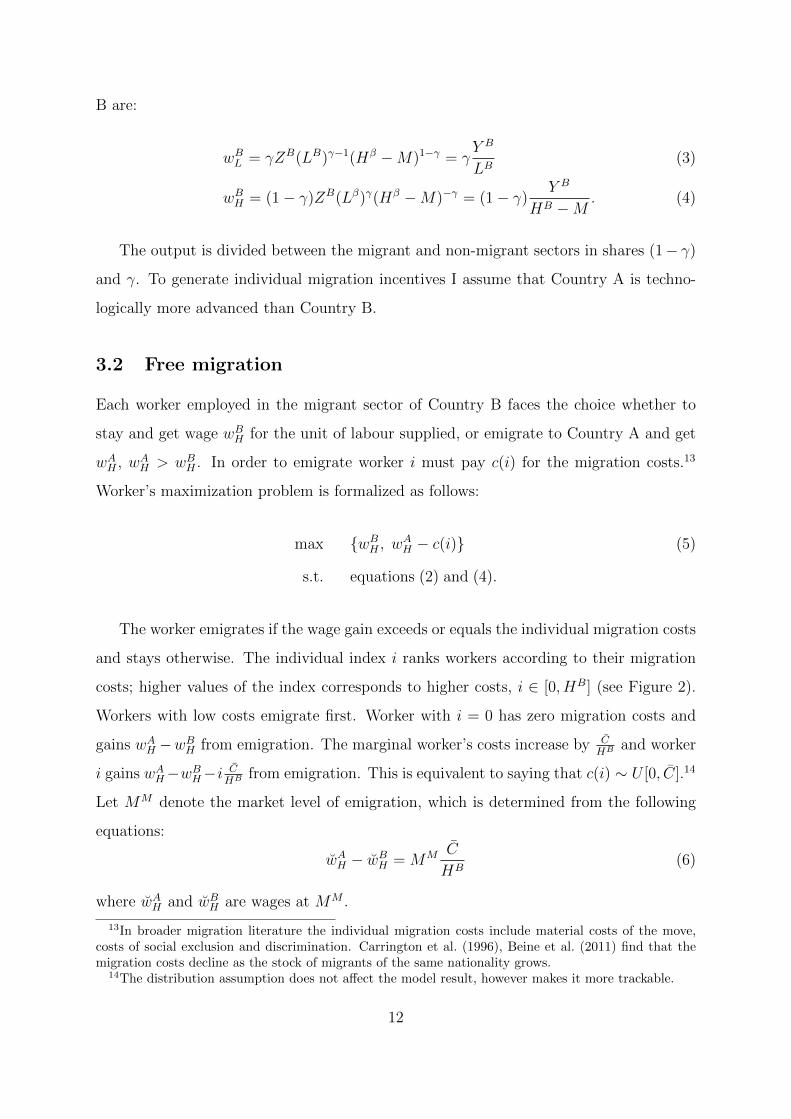
The worker emigrates if the wage gain exceeds or equals the individual migration costs
and stays otherwise. The individual index i ranks workers according to their migration
costs; higher values of the index corresponds to higher costs, i ∈ [0, HB] (see Figure 2).
Workers with low costs emigrate first. Worker with i = 0 has zero migration costs and
gains wAH −wBH from emigration. The marginal worker’s costs increase by CHB and worker
i gains wAH−wBH−i CHB from emigration. This is equivalent to saying that c(i) ∼ U [0, C].14
Let MM denote the market level of emigration, which is determined from the following
equations:
wAH − wBH = MM C
HB(6)
where wAH and wBH are wages at MM .
13In broader migration literature the individual migration costs include material costs of the move,costs of social exclusion and discrimination. Carrington et al. (1996), Beine et al. (2011) find that themigration costs decline as the stock of migrants of the same nationality grows.
14The distribution assumption does not affect the model result, however makes it more trackable.
12

0
C
HB
slope = CHB
MMi
c(i)
c
Figure 2: Visualization of individual migration costs.
Given the migration level MM and the assumption of the uniform distribution of the
costs, the total migration costs paid, which is the area of triangular below the diagonal
line in Figure 2, equal (MM )2C2HB .
If Country A becomes relatively more technologically developed, ceteris paribus, MM
will increase. If Country A employs more people in the migrant sector, the wage in that
sector declines thus reducing MM . If C increases, the average migration costs increase,
thus resulting in less migration. MM does not depend on the total population in both
countries, however it does depend on the distribution of workers across the two sectors.
It must further be noted, that the individual decision rule in equation (5) accounts for
the fact that in the migrant sector a moving worker decreases the wage in Country A and
increases the wage in Country B. This however ignores a number of the welfare effects,
for example, change in income of native and migrant workers induced by the change in
wages (Card, 1990; Bratsberg and Raaum, 2012) as well as the social costs incurred from
immigration (Giordani and Ruta, 2011).
13

3.3 Country A preference
Country A maximizes the welfare of its native workers by choosing the volume of migrants
M to accept for employment in the migrant sector. The maximization problem is defined
as follows:
max{M}
WA (M) = LAwAL +HAwAH −A
2
(M
NA
)2
NA (7)
s.t. equations (1) and (2)
M ≥ 0.
The first two terms of the welfare function is the income that accrues to the native
workers minus wages paid to migrants. The third term is the social immigration costs
incurred by the receiving country.15 This term expresses in monetary terms the value
of all costs that the country incurs from accepting migrant workers: border controls
and policing, integration and language courses or simply the natives’ dissatisfaction from
having migrants around.
The welfare effect of immigration is derived by differentiating (7) w.r.t. M . After
rearrangement I obtain:
∂WA
∂M= LA
∂wAL∂M
+HA∂wAH
∂M− A
NAM =
βwAHNA
(1− HA
HA +M
)− A
NAM.
SinceβwAHNA
(1− HA
HA+M
)> 0 for M > 0, the natives’ income is strictly increasing in
the number of migrants. Disregarding the social costs, the native workers are strictly
better off from the marginal migrant. To see why it is so, consider the migrant’s effect
on output:
wAH =∂Y A
∂M=
∂
∂M
(LAwAL +
(HA +M
)wAH)
= LA∂wAL∂M
+HA∂wAH
∂M+M
∂wAH∂M
+ wAH .
A migrant is paid his marginal product and his arrival generates two more effects
which cancel out: a positive effect on wage in the non-migrant sector and a negative
15Giordani and Ruta (2011) use s different functional form for the costs, but the function propertiesremain the same.
14

effect on wage in the migrant sector.
LA∂wAL∂M
+HA∂wAH
∂M︸ ︷︷ ︸effect on natives, > 0
+ M∂wAH∂M︸ ︷︷ ︸
effect ondiaspora, ≤ 0
= 0. (8)
The negative effect on the wage in the migrant sector reduces the income of the native
and migrant workers. Reduction of the natives’ income is smaller in absolute value than
the increase in the non-migrant sector. For this reason, disregarding the social costs,
immigration always increases the natives’ income. The positive effect on the locals is
referred to in the literature as the “immigration surplus” (Borjas, 1995b; Giordani and
Ruta, 2011).
The third term in equation (8) is the effect of migrants on their own income, which I
call the diaspora effect. This effect is defined to be:
M∂wAH∂M
= 0 if M = 0
< 0 if M > 0.
The diaspora effect does not affect the welfare of Country A, because the migrants
take away the negative effect on themselves. The diaspora effect in a crucial way affects
the welfare of Country B, which is considered in detail in Section 3.4.
It costs ANA in social costs to accepts the marginal migrant. The welfare effect of
immigration is:
∂WA
∂M
= 0 if M = 0
≥ 0 ifβwAHNA
(1− HA
HA+M
)≥ A
NAM
< 0 ifβwAHNA
(1− HA
HA+M
)< A
NAM.
When there are no migrants in Country A, M = 0, the first migrant does not generate
the diaspora effect, therefore the effect on the locals is zero. When migration continues,
the marginal migrant positively affects the natives’ income, and negatively affects the
income of migrants already in the country through the diaspora effect. Country A will
continue to accept migrants until the marginal increase in the natives’ income equalizes
with the marginal increase in the social costs. The last migrant allowed in increases the
15

locals’ income by strictly as much as he increases the social costs.
Denote the optimal volume of migrants that solves maximization problem (7) by
MA. Using the welfare effects as the sole determinant of the immigration policy, two
immigration policy profiles of Country A are considered:
1. Immigration quota:
MA =
[NAZAβ(1− β)(LA)β
A
] 11+β
−HA (9)
2. Immigration ban:
MA = 0.
The immigration quota defines the immigration volume that maximizes the welfare
of Country A. It can happen that the quota is not exhausted, in which case the first-best
outcome is not achieved. The country will not accept more than the quota, because
of the social costs. The quota is strictly increasing in the total workforce, NA, total
factor productivity, ZA, and decreasing in the social cost parameter A. When the native
workforce is predominantly employed in the non-migrant sector, the country accepts many
migrants, because the welfare can be increased by extending employment in the migrant
sector. The immigration quota MA is concave in β. For low values of β the migrant
sector is more important in production and has a high marginal effect on the welfare.
As β increases the marginal effect on the quota is positive until a certain point, after
which it becomes negative. For small and large values of β the quota is smaller than for
intermediate values.
When migrants do not cause any social costs, i.e. A = 0, the country accepts infinitely
many migrants, because the marginal effect on the natives’ income is strictly positive, as
derived in equation (8). Similar “open door” immigration policy predictions are confirmed
by Bianchi (2013) and Giordani and Ruta (2011).
16

3.4 Country B preference
Migrant workers come to Country A from a less developed Country B. If Country B
could choose how many emigrants to send, it would do so by maximizing the welfare of
its emigrants and stayers. It thus solves the following maximization problem:
max{M}
WB (M) = MwAH −MMC
2HB+ LBwBL +
(HB −M
)wBH (10)
s.t. equations (1), (2), (3) and (4)
M ≥ 0.
The first term of the welfare function is the income of migrants, the second term is
the total individual migration costs, the third and fourth terms are the income of stayers
in Country B. To learn the welfare effects of emigration I have to differentiate (10) w.r.t.
M . After rearrangement I obtain:
∂WB
∂M= wAH − wBH −
MC
HB︸ ︷︷ ︸net gain fromemigration
+ M∂wAH∂M︸ ︷︷ ︸
diasporaeffect, ≤ 0
+LB∂wBL∂M
+(HB −M
) ∂wBH∂M︸ ︷︷ ︸
effect on stayers, = 0
. (11)
Starting from no emigration, M = 0, the first migrant gains wAH , looses wBH and pays
nothing in migration costs. For the first migrant, the diaspora effect is zero, because no
migrants in Country A are affected by the wage reduction. For M > 0 each marginal
migrant will reduce the wage paid to the first migrant, thus generating the negative
diaspora effect.
Emigration has two effects on stayers; increase of wage in the migrant sector and
decrease of wage in the non-migrant sector. These two effects cancel out:
−wBH =∂Y B
∂M=
∂
∂M
(LBwBL +
(HB −M
)wBH)
= LB∂wBL∂M
+(HB −M
) ∂wBH∂M
− wBH .
17

The welfare effect of emigration on Country B is thus:
∂WB
∂M
= wAH − wBH if M = 0
≥ 0 if wAH − wBH ≥ MCHB −M
∂wAH∂M
and M > 0
< 0 if wAH − wBH < MCHB −M
∂wAH∂M
and M > 0.
The first migrant increases welfare by exactly as much as his net private gain from
emigration. From then on, each marginal migrant increases the welfare by less than the
private gain from emigration because of the negative diaspora effect. As the number
of migrants increases, the marginal welfare gain declines, because the wage differential
narrows, the individual migration costs increase and the diaspora effect grows. The
country prefers to send migrants as long as the wage differential exceeds the marginal
migration costs and the marginal decline in income of the diaspora. The wage gain for
the last migrant that Country B wants to send exactly equals the marginal migration
costs plus the marginal increase in the diaspora effect.
I use MB to denote the emigration level that solves maximization problem (10) and
wAH , wBH to denote wages at MB. Two emigration profiles of Country B are considered:
1. Emigration quota:
wAH − wBH =MBC
HB+MB βwAH
HA +MB(12)
2. Emigration ban:
MB = 0.
Comparing equations (12) and (6) one can notice that they differ only by the term
that captures the diaspora effect. This means that for M > 0 Country B always prefers
to have fewer migrants than the volume that self-establishes under free migration.
The emigration quota depends on the sectoral distribution of workers. Larger employ-
ment in the migrant sector in County A (B) will reduce (increases) the wage differential,
thus driving down (up) the emigration quota. If ZA(ZB)
increases, MB will increase (de-
crease), because the difference in wages rises (falls). If the average migration costs decline,
i.e. C falls, Country B prefers to have more migrants.
18

3.5 Political union preference
Suppose that the two countries form a political union. It is then interesting to know how
many migrants the union would like to have. The union solves the following maximization
problem:
max{M}
WU (M) = LAwAL +HAwAH −A
2
(M
NA
)2
NA +MwAH −MMC
2HB+ (13)
+ LBwBL +(HB −M
)wBH
s.t. equations (1), (2), (3) and (4)
M ≥ 0.
The first three terms of the objective function is the income that accrues to the natives
of Country A, net wages paid to migrants and the social immigration costs. The fourth
and fifth terms are the migrants’ income minus the migration costs. The second line is
the income of stayers in Country B.
To learn the welfare effects of migration I have to differentiate (13) w.r.t. M . After
rearrangement I obtain:
∂WU
∂M= LA
∂wAL∂M
+HA∂wAH
∂M+M
∂wAH∂M︸ ︷︷ ︸
=0
+wAH − wBH −MA
NA︸ ︷︷ ︸net gain fromemigration
−M C
HB︸ ︷︷ ︸socialcost
+
+LB∂wBL∂M
+HB ∂wBH
∂M−M∂wBH
∂M︸ ︷︷ ︸effect on stayers’ income, = 0
.
The marginal migrant with index i gains wAH , looses wBH and pays i CHHB for the im-
migration costs. For accepting this migrant the union pays ANA in the form of social
costs. The marginal net gain to the union is thus wAH −wBH − i CHHB − ANA . Since the union
cares about the welfare of all its workers irrespective of their country profile, migrants
stop being migrants and the pronounced diaspora effect is internalized as it is shown in
equation (8).
The union prefers to have migrants as long as the wage gain from migration exceeds
the marginal individual and social costs. For the last migrant the wage gain will exactly
19

equal the marginal individual and social costs. The welfare effect of migration in the
union is as follows:
∂WU
∂M
= wAH − wBH − A
NA if M = 0
≥ 0 if wAH − wBH ≥ MCHB + A
NAM and M > 0
< 0 if wAH − wBH < MCHB + A
NAM and M > 0.
Let MU denote the optimal migration level within the union, wAH and wBH denote
wages at MU . Then two migration profiles of the union are considered:
1. Migration quota:
wAH − wBH =MU CHHB
+A
NAMU (14)
2. Migration ban:
MU = 0.
The union migration policy is the weighted average of the individual migration profiles
of the two countries. If Country A accepts migrants more aggressively than Country B
wishes to send them, the optimal volume for the union will be below that of Country A
and above than of Country B. In the opposite case, when Country A wishes to accepts
less migrants than Country B wants to send, the union preference will be above that of
Country A and below that of Country B.
When the social costs of immigration are reduced to zero, A = 0, the union prefer-
ence equals the free market outcome, because the migrants in the union do not impose
any negative effects on the income of other migrants. This intuition is formalized in
Proposition 1.
20

3.6 Comparison of outcomes
In this section I compare the four migration outcomes: free market, preference of Coun-
try A, preference of Country B and preference of the political union. As a starting point,
let me recall the optimal migration levels:
Market: wAH − wBH =MM C
HB(15)
Country A: βwAH
(1− HA
HA +MA
)=AMA
NA(16)
Country B: wAH
(1− βMB
HA +MB
)− wBH =
MBC
HB(17)
Union: wAH − wBH =MU C
HB+AMU
NA(18)
where wSH , wSH , wSH and wSH , S = A,B, are wages in migrant sectors at respective migra-
tion levels. The four outcomes are depicted in Figure 3.
0.5 10.05
0.15
A
M
MM
MA
MB
MU
A2
A1
Figure 3: Illustration of the migration outcomes for the following parameter values:ZA = 2, ZA = 1.5, NA = NB = 1, HA = HB = 0.5, β = γ = 0.5, C = 0.15.
The immigration quota MA defines the volume of immigrants that is best for the
receiving Country A. When the social immigration cost parameter A declines, the country
accepts more migrants.
21

The market outcome defines a migration level when workers are allowed to move freely.
The worker’s decision to move, as given by maximization problem (5), weights the wage
differential against the marginal migration costs. It ignores the social immigration costs
and the negative effect of migrants on their own income through the diaspora effect.
The preference of County B defines the volume of migrants that is best for its welfare,
which consists of the income of workers in the non-migrant sector, stayers in the migrant
sector and the emigrants. When the wage differential is sufficiently high, Country B can
increase its welfare by expatriating some of its workers to work in Country A where they
are more productive. As the number of emigrants increases, the wage in the destination
country falls, thus decreasing the income of migrants (diaspora effect). The optimal
emigration quota for Country B is when the wage differential equals the marginal decrease
in the migrants’ income plus the marginal migration costs. This compares to the market
migration level, which disregards migrants’ effect on their own income. Proposition 1
shows that the negative diaspora effect decreases the optimal volume of migrants for the
source country relative to the free market level.
The union outcome describes the case when both countries can agree on such a level
of migration, which is best for the world. The union quota is thus a weighted average of
the preferences of sending and receiving countries; it accounts for the wage differential,
social and individual costs as well as the negative diaspora effect. Since in the union
migrant workers stop being migrants (their well-being is cared for by the planner) the
negative diaspora effect is internalized. For this reason Country B always benefits from
coordination.
Two propositions below rank the migration outcomes depending on the value of the
social cost parameter.
22

Proposition 1. If A = 0, the outcomes are ranked MA > MM = MU > MB.
Proof. If A = 0, then from equations (9) or (16) it follows that MA → ∞. Next,
MM = MU because equations (15) and (18) are the same. Further, I subtract equation
(15) from (17) to obtain:
wAH
(1− βMB
HA +MB
)− wAH + wBH − wBH =
C
HB
(MB −MM
)(19)
If MB > MM , then the LHS of (19) is negative but the RHS is positive, which is a
contradiction. If MB = MU , then the LHS is negative but the RHS = 0, which is again
a contradiction. Then MB < MM is the true relationship, because it does not produce a
contradiction.
By the transitivity property the ranking MA > MM = MU > MB follows.
Proposition 1 establishes the first key result of the paper – over-emigration. If workers
are allowed to move freely, the market outcome delivers more migrants than the quota of
Country B, MM > MB. In other words, more people move than is optimal for the source
country. Compared to findings of the brain drain literature, this result suggests that
emigration of a marginal worker decreases output in the sending country by the worker’s
wage; emigration does not decrease the income of stayers; and, finally, the emigration
of MM −MB extra migrants is harmful to the source country, because they excessively
decrease the income of MM migrants who are already in the destination country.
Further, since the union preference internalizes the negative diaspora effect and when
the social immigration costs are zero, the union quota equals the free market level of
migration. The political union prefers to have as many migrants as workers who wish
to move. This result also follows from the application of the First Welfare Theorem.
In the absence of social immigration costs the receiving country prefers the open door
immigration policy, because the marginal benefit of an additional migrant is strictly
positive. This result is not uncommon in the literature; Giordani and Ruta (2011) and
Bianchi (2013) are most recent studies that confirm it.
23

Proposition 2. There exist A1 and A2, such that:
MA > MM > MU > MB if A < A1 (20)
MM > MA > MU > MB if A1 < A < A2 (21)
MM > MB > MU > MA if A > A2. (22)
Proof. The three cases are depicted in Figure 3. It follows from Proposition 1 that MM
and MA do not depend on A, they are parallel lines with MM above MB, ∂MM
∂A= ∂MB
∂A=
0, MM > MB.
MA is a continuous function decreasing in A. For small values of A MA is above
MM and for large values MA is below MB. There exist a unique point A1 at which MA
intersects MM , such that if A < A1, MA > MM , and conversely, if A > A1, MA < MM .
Similarly, there exist a unique point A2 at which MA intersects MB, such that if A < A2,
MA > MB, and, conversely, if A > A2, MA < MB. Since MA is a downward sloping
line, it first crosses MM and then MB, A1 < A2.
MU is a continuous function decreasing in A. For A = 0 MU = MM (Proposition 1),
and for A > 0 MU < MM . For small values of A MU > MB, and for large values
MU < MB. There exists a point at which MU crosses MB and this point is unique. If
I add equations (16) and (17) I get equation (18), which implies that MA, MU and MB
intersect in one point, A2. If A < A2, MU lies below MA but above MB, MA > MU >
MB, and conversely, if A > A2, MB > MU > MA.
Conditions (20)–(22) are depicted in Figure 3. Condition (20) describes the case
when due to low social immigration costs the immigration quota is set high enough and
it exceeds three other outcomes. In this case the quota will not be exhausted, because
less migrants wish to move under the free migration.
When condition (21) holds the social cost parameter is high enough and brings the
immigration quota below the market level. This establishes the second key result of the
paper. Given the finding of over-emigration, enforcement of the immigration quota by
the host country benefits the welfare of the source country, because it reduces the volume
of excessive migrants from MM −MB to MA−MB, thus reducing the negative diaspora
effect. Contrary to the well-acknowledged opinion, that developed countries should accept
24

more migrants to increase the welfare in the developing source region, if condition (21)
holds, enforcement of the quota actually benefits the source country.
If condition (22) holds, the social immigration costs are too high and the immigration
quota is set too low. If the quota is enforced, there will be rationing of migrants and
under-emigration with respect to what is best for the source country, the union and the
market.
3.7 Comparison with brain drain
The brain drain literature finds that emigration of skilled workers decreases the welfare
of those left behind and reduces economic growth in sending countries (Bhagwati and
Hamada, 1974; Bhagwati and Hamada, 1982; Dustmann et al., 2011; Mountford and
Rapoport, 2011). In comparison this result establishes that if the welfare of the will-
be migrants while they are in Country B is accounted for, the effect on stayers is zero.
However, if the will-be migrants are excluded from the welfare, then for given M the
marginal effect on stayers is negative.
The marginal effect of emigration on stayers and will-be migrants from equation (11)
is:
LB∂wBL∂m
+(HB −m
) ∂wBH∂m
= 0. (23)
The total effect is also zero:
∫ M
0
LB∂wBL∂m
+(HB −m
) ∂wBH∂m
dm = 0. (24)
Suppose now that a social planner knows M in advance and wishes to compute the
welfare effect on stayers excluding the will-be migrants while they are still in Country B.
The marginal effect is then:
LB∂wBL∂m
+(HB −M
) ∂wBH∂m
< 0 for M > m. (25)
For M > m the marginal effect in equation (25) is negative, and for M = m it is zero.
25

The total effect is therefore negative and given by:
∫ M
0
LB∂wBL∂m
+(HB −M
) ∂wBH∂m
dm < 0. (26)
Unlike the brain drain literature, the non-positive effect on the welfare of stayers holds
for emigration of workers of any skill level and from any migrant sector of Country B:
medical professionals, construction workers, computer scientists or cleaners.
4 Conclusions
In this paper I analyze the welfare effects of migration for three parties involved: migrants,
receiving country and sending country. As stated in many studies, workers move in
response to the wage differential between countries after deducing individual migration
costs. Thus, when deciding to move, individual workers disregard their effect on the host
and source countries’ welfare as well as other migrants. The free migration level confronts
the immigration quota of the receiving country; all prospective migrants move as long as
the market level is below the quota, and the prospective migrants are rationed when the
quota is below the market level.
In the absence of social immigration costs, immigration strictly benefits the receiving
country. When these costs are not zero, the immigration quota is determined when the
marginal increase in the host country workers’ income equals the marginal increase in the
social costs.
For the source country, emigration is found to decrease the output by the worker’s
wage. This however does not affect the income of stayers. I find that there is always over-
emigration with respect to what is optimal for the source country, because the individual
decision rule does not account for the migrants’ effect on their own income (diaspora
effect), which is negative since migrants cluster in the same employment sector. Over-
emigration is harmful to the source country welfare. Under certain conditions the negative
impact of over-emigration can be reduced when the destination country enforces the
quota.
The source country prefers to coordinate the immigration quota with the host country,
26

because in the coordinated outcome of the political union the migrant workers stop being
migrants and the negative diaspora effect is internalized. When the social immigration
costs are zero, the union quota delivers the same outcome as the free market.
27

Appendix
Table 1: Standardized migration statistics.
AU
T
BE
L
CZ
E
HU
N
GB
R
FIN
FR
A
US
A
CH
E
DE
U
GR
C
LU
X
DN
K
IRL
SW
E
ITA
NO
R
NL
D
PR
T
ES
P
Permanent inflows and outflows in 2010, per one thousand of local population*Inflows 11.7 10.4 2.9 2.4 8.1 3.4 2.2 3.4 17.2 8.4 2 31.5 6 3.9 8.4 7.1 13.3 6.6 2.8 9.4Outflows 7.9 . 1.4 0.6 3.3 0.6 . . 8.4 8.2 4.2 15.2 4.9 8.4 2.4 0.5 4.6 2.4 . 7.3
Inflows in 2011 by category of entry, %Work 1.4 18.3 . . 33.1 5.8 11.9 6.4 2.1 9.0 . . 19.6 16.3 5.7 40.5 5.1 10.9 21.9 29.9Free movements 63.7 39.6 . . 17.4 39.0 30.3 0.0 71.4 59.9 . . 50.9 71.8 35.9 28.2 67.4 56.9 36.3 49.9Accompanying family 0.9 0.0 . . 14.6 0.0 0.0 7.8 0.0 0.0 . . 5.9 4.0 0.0 1.2 0.0 0.0 0.0 0.0Family 23.2 36.2 . . 11.8 34.3 42.9 66.3 18.8 24.7 . . 12.3 7.0 39.6 27.4 18.0 21.7 35.3 18.7Humanitarian 10.3 5.9 . . 1.2 17.4 5.4 13.1 5.8 5.3 . . 5.1 0.9 18.7 1.3 9.5 10.5 0.1 0.2Other 0.5 0.0 . . 21.9 3.6 9.6 6.4 2.0 1.1 . . 6.2 0.0 0.0 1.5 0.0 0.0 6.3 1.2
Stock of migrants in 2010, % of populationForeign-born 15.7 13.9 6.3 4.5 11.5 4.6 8.6 12.2 26.6 13 10.9 37.6 7.7 17.3 14.8 8 11.6 11.2 . 14.5Foreign nationals 11.1 9.8 4 2.1 7.4 3.1 6 7 22.1 8.3 7.1 44.1 6.2 . 6.8 7.6 7.6 4.6 4.2 12.4
Unemployment rate in 2011, %Native-born 3.4 5.8 6.8 11.1 8 7.6 8.5 9.2 3.1 5.4 17.4 3.4 6.9 14.1 6 8 2.7 3.8 13 19.5Foreign-born 8.2 15.1 8 9.5 9.4 15.2 15.1 9.1 6.8 9.5 22.2 6.3 14.5 17.3 16 11.7 7.7 9.2 16.9 31.5Share of foreign-bornin tot. empl., %, 2010 16.5 13.0 2.8 2.1 13.3 3.8 11.1 15.8 27.2 14.3 11.5 48.7 9.4 17.2 14.4 11.8 9.5 11.3 9.1 17.0
Difference in education level shares: recent migrants (2000–2010) minus young resident workers**Low 16.4 18.0 6.9 2.3 14.1 29.4 23.9 26.4 11.8 17.7 41.9 1.0 . 9.0 20.7 28.9 . 17.6 11.1 13.3Medium -21.2 -7.3 -4.2 -8.6 6.1 -6.6 -12.4 -12.0 -22.0 -31.2 -8.8 -26.5 . 3.8 -28.8 -12.0 . -10.1 8.9 13.3High 4.7 -10.7 -2.8 6.4 -20.2 -22.8 -11.6 -14.4 10.1 13.5 -33.1 25.4 -11.8 -12.8 8.1 -17.0 -11.5 -7.5 -20.0 -26.6
Source: author’s illustration using data from OECD (2011) and OECD (2012).
* National definitions of migrant.
** “Low” refers to less than upper secondary attainment, “medium” to upper secondary and post-secondary non-tertiary, “high” to tertiary.
A dot means that the data are unavailable or the estimate is unreliable.
28

Table 2: Migrants’ employment by sector and occupation group.
Au
stri
a
Bel
giu
m
Cze
chR
ep.
Hu
ngary
UK
Fin
lan
d
Fra
nce
US
Sw
itze
rlan
d
Ger
many
Gre
ece
Lu
xem
bou
rg
Den
mark
Irel
an
d
Sw
eden
Italy
Norw
ay
Net
her
lan
ds
Port
ugal
Sp
ain
Distribution of migrants across employment sectors in 2011*, %Agriculture and fishing 0.9 0.6 1.2 . 0.5 2.6 1.3 2.2 1.2 0.7 8.9 . 2.4 2.2 0.6 4.0 . 1.7 . 5.7Mining, manufacturingand energy 17.8 13.3 31.1 23.9 10.6 15.3 11.7 12.9 18.4 25.6 13.4 6.8 13.9 17.1 13.2 20.6 12.0 14.5 14.1 9.3Construction 11.8 9.6 10.1 7.9 5.7 6.1 12.3 9.3 8.0 7.0 19.2 9.9 1.8 4.2 4.1 13.6 6.2 4.2 9.9 10.5Wholesale and retail trade 14.6 11.8 15.1 16.1 13.2 12.8 11.7 13.9 14.2 12.7 14.6 10.8 11.8 16.3 11.1 10.1 11.2 12.6 13.3 13.6Hotels and restaurants 12.1 8.2 5.6 5.7 9.2 8.5 7.0 10.5 7.7 8.8 12.1 5.9 7.5 11.7 7.2 8.8 6.8 6.8 10.5 16.1Education 4.3 5.5 5.2 9.8 8.2 8.1 5.2 5.8 5.3 4.5 1.5 4.1 9.5 4.9 11.3 1.9 6.5 6.6 9.1 2.2Health 9.5 10.9 4.6 9.4 15.6 11.7 11.6 12.1 13.1 10.7 3.2 7.4 21.5 14.4 19.3 4.8 24.3 16.4 7.2 5.0Households . 2.2 . . 0.4 . 5.4 1.4 1.3 1.1 14.7 3.5 . 1.0 . 17.0 . . 5.1 14.9Administrative 2.6 9.9 3.1 4.5 4.1 2.5 6.4 2.4 2.2 2.4 0.9 14.4 3.2 2.2 3.7 1.4 3.0 6.3 7.1 2.0Other services 25.8 28.0 23.9 20.1 32.4 32.3 27.5 29.5 28.6 26.6 11.5 37.0 28.0 26.0 29.4 17.7 28.5 30.8 22.2 20.6
Difference in occupation shares: recent migrants (2000–2010) minus young resident workersElementary occupations 17.1 11.4 9.4 1.8 10.6 17.9 15.2 14.6 4.7 14.3 38.7 3.1 19.2 17.7 12.5 34.2 14.2 16.2 24.6 34.0Clerks, service workers, skilledtrades, machinery operators -1.2 -1.7 5.4 -4.2 3.3 0.6 3.0 1.7 -5.3 2.6 0.8 -7.4 3.8 18.5 -1.4 -1.0 5.8 7.4 5.5 2.9Professionals, seniorofficials and managers 1.9 -5.6 -0.8 11.7 -7.5 -6.0 -2.9 -16.3 11.9 -2.4 -25.4 14.3 -8.6 -28.8 -1.1 -9.3 -3.8 -13.8 -18.3 -20.3Technicians andassociate professionals -17.8 -4.1 -14.1 -9.3 -6.5 -12.6 -15.3 0.0 -11.3 -14.5 -14.1 -10.0 -14.4 -7.4 -9.9 -23.9 -16.3 -9.7 -11.8 -16.5
Source: author’s illustration using data from OECD (2012).
* ISIC classification, rev.3.
A dot means that the data are unavailable or the estimate is unreliable.
29

References
Akin, S., 2012. Immigration, fiscal policy, and welfare in an aging population. The B.E.
Journal of Macroeconomics (advances) 12 (1).
Batista, C., Lacuesta, A., Vicente, P., 2012. Testing the brain gain hypothesis: micro
evidence from Cape Verde. Journal of Development Economics 97 (1), 32–45.
Beine, M., Docquier, F., Ozden, C., 2011. Diasporas. Journal of Development Economics
95 (1), 30–41.
Benhabib, J., 1996. On the political economy of immigration. European Economic Review
40 (9), 1737–1743.
Bertoli, S., Brucker, H., 2011. Selective immigration policies, migrants’ education and
welfare at origin. Economics Letters 113 (1), 19–22.
Bhagwati, J., Hamada, K., 1974. The brain drain, international integration of markets
for professionals and unemployment: a theoretical analysis. Journal of Development
Economics 1 (1), 19–42.
Bhagwati, J., Hamada, K., 1982. Tax policy in the presence of emigration. Journal of
Public Economics 18 (3), 291–317.
Bianchi, M., 2013. Immigration policy and self-selecting migrants. Journal of Public Eco-
nomic Theory 15 (1), 1–23.
Billet, C., 2010. EC readmission agreements: A prime instrument of the external dimen-
sion of the eus fight against irregular immigration. an assessment after ten years of
practice. European Journal of Migration and Law 12 (1), 45–79.
Borjas, B., 1987a. Self-selection and the earnings of immigrants. American Economic
Review 77 (4), 531–553.
Borjas, G., 1995a. The economic benefits from immigration. Journal of Economic Per-
spectives 9 (2), 3–22.
30

Borjas, G. J., 1987b. Immigrant, minorities, and labor market competition. Industrial
and labor relations review 40 (3), 382–392.
Borjas, G. J., 1995b. The economic benefits from immigration. Journal of Economic
Perspectives 9 (2), 3–22.
Borjas, G. J., 2011. Poverty and program participation among immigrant children. The
Future of Children 21 (1), 247–266.
Bratsberg, B., Raaum, O., 2012. Immigration and wages: Evidence from construction.
Economic Journal 122 (565), 1177–1205.
Burda, M., Wyplosz, C., 1992. Human capital, investment and migration in an integrated
Europe. European Economic Review 36 (23), 677–684.
Card, D., 1990. The impact of the Mariel boatlift on the Miami labor market. Industrial
and Labor Relations Review 43 (2), 245–257.
Carrington, W. J., Detragiache, E., Vishwanath, T., 1996. Migration with endogenous
moving costs. American Economic Review LXXXVI, 909–930.
Cellini, R., 2007. Migration and welfare: a very simple model. Journal of International
Development 19 (7), 885–894.
Clark, X., Hatton, T., Williamson, J., 2007. Explaining US immigration, 1971-1998.
Review of Economics and Statistics 89 (2), 359–373.
Docquier, F., Rapoport, H., Salomone, S., 2012. Remittances, migrants’ education and
immigration policy: Theory and evidence from bilateral data. Regional Science and
Urban Economics 42 (5, SI), 817–828.
Dustmann, C., Fadlon, I., Weiss, Y., 2011. Return migration, human capital accumulation
and the brain drain. Journal of Development Economics 95 (1), 58–67.
Filer, R., May 1992. The effect of immigrant arrivals on migratory patterns of native
workers. In: Immigration and the Workforce: Economic Consequences for the United
States and Source Areas. NBER Chapters. National Bureau of Economic Research,
Inc, pp. 245–270.
31

Frontex, 2011. General report 2011. Tech. rep., Frontex.
Fuest, C., Thum, M., 2000. Welfare effects of immigration in a dual labor market. Regional
Science and Urban Economics 30 (5), 551–563.
Gera, S., Songsakul, T., 2007. Benchmarking Canada’s performance in the global compe-
tition for mobile talent. Canadian Public Policy – Analyse de politiques 33 (1), 63–84.
Giordani, P. E., Ruta, M., 2011. The immigration policy puzzle. Review of International
Economics 19 (5), 922–935.
Heckman, J. J., 1979. Sample selection bias as a specification error. Econometrica 47 (1),
153–161.
Ketkar, S. L., Ratha, D., 2010. Diaspora bonds: tapping the diaspora during difficult
times. Journal of International Commerce, Economics and Policy 01 (02), 251–263.
LaLonde, R. J., Topel, R. H., 1991. Immigrants in the American labor market: quality,
assimilation, and distributional effects. American Economic Review 81 (2), 297–302.
Marchiori, L., Shen, I.-L., Docquier, F., 2013. Brain drain in globalization: a general
equilibrium analysis from the sending countries’ perspective. Economic Inquiry 51 (2),
1582–1602.
Mattoo, A., Neagu, I. C., Ozden, C., 2008. Brain waste? Educated immigrants in the US
labor market. Journal of Development Economics 87, 255–269.
Mavroudi, E., Warren, A., 2013. Highly skilled migration and the negotiation of immigra-
tion policy: Non-EEA postgraduate students and academic staff at English universities.
GEOFORUM 44, 261–270.
Miller, P. W., 1999. Immigration policy and immigrant quality: the Australian points
system. American Economic Review 89 (2), 192–197.
Mincer, J., 1978. Family migration decisions. Journal of Political Economy 86 (5), 749–
773.
32

Mountford, A., 1997. Can a brain drain be good for growth in the source economy?
Journal of Development Economics 53 (2), 287–303.
Mountford, A., Rapoport, H., 2011. The brain drain and the world distribution of income.
Journal of Development Economics 95 (1), 4–17.
OECD, 2011. International Migration Outlook. OECD Publishing, Paris.
OECD, 2012. International Migration Outlook. OECD Publishing, Paris.
OECD, 2013. Recruiting Immigrant Workers: Germany 2013. OECD Publishing.
Ortega, F., Peri, G., 2009. The causes and effects of international migrations: evidence
from OECD countries 1980-2005. NBER Working paper No. 14833.
Ostrovsky, Y., 2012. The dynamics of immigrant participation in entitlement programs:
evidence from Canada, 1993–2007. Canadian Journal of Economics/Revue canadienne
d’economique 45 (1), 107–136.
Rabe, B., 2011. Dual-earner migration. earnings gains, employment and self-selection.
Journal of Population Economics 24, 477–497.
Razin, A., Sadka, E., 1999. Migration and pension with international capital mobility.
Journal of Public Economics 74 (1), 141–150.
Schiff, M., 2002. Love thy neighbor: trade, migration, and social capital. European Jour-
nal of Political Economy 18 (1), 87–107.
Stark, O., Helmenstein, C., Prskawetz, A., 2004. Rethinking the brain drain. World
Development 32 (1), 15–22.
Storesletten, K., 2000. Sustaining fiscal policy through immigration. Journal of Political
Economy 108 (2), 300–323.
United Nations, 2011. International migrant stock by origin: the 2010 revision. Population
Division, Migration Section.
Zimmermann, K. F., 1995. Tackling the European migration problem. Journal of Eco-
nomic Perspectives 9 (2), 45–62.
33

Working Paper Series ISSN 1211-3298 Registration No. (Ministry of Culture): E 19443 Individual researchers, as well as the on-line and printed versions of the CERGE-EI Working Papers (including their dissemination) were supported from institutional support RVO 67985998 from Economics Institute of the ASCR, v. v. i. Specific research support and/or other grants the researchers/publications benefited from are acknowledged at the beginning of the Paper. (c) Dmytro Vikhrov, 2013 All rights reserved. No part of this publication may be reproduced, stored in a retrieval system or transmitted in any form or by any means, electronic, mechanical or photocopying, recording, or otherwise without the prior permission of the publisher. Published by Charles University in Prague, Center for Economic Research and Graduate Education (CERGE) and Economics Institute of the ASCR, v. v. i. (EI) CERGE-EI, Politických vězňů 7, 111 21 Prague 1, tel.: +420 224 005 153, Czech Republic. Printed by CERGE-EI, Prague Subscription: CERGE-EI homepage: http://www.cerge-ei.cz Phone: + 420 224 005 153 Email: [email protected] Web: http://www.cerge-ei.cz Editor: Michal Kejak The paper is available online at http://www.cerge-ei.cz/publications/working_papers/. ISBN 978-80-7343-295-9 (Univerzita Karlova. Centrum pro ekonomický výzkum a doktorské studium) ISBN 978-80-7344-287-3 (Národohospodářský ústav AV ČR, v. v. i.)