DM554 Linear and Integer Programming - SDUmarco/Teaching/AY2014-2015/...DM554 Linear and Integer...
46
DM554 Linear and Integer Programming Lecture 9 Diagonalization Marco Chiarandini Department of Mathematics & Computer Science University of Southern Denmark
Transcript of DM554 Linear and Integer Programming - SDUmarco/Teaching/AY2014-2015/...DM554 Linear and Integer...
DM554
Linear and Integer Programming
Lecture 9Diagonalization
Marco Chiarandini
Department of Mathematics & Computer ScienceUniversity of Southern Denmark

Coordinate ChangeDiagonalizationApplicationsOutline
1. More on Coordinate Change
2. Diagonalization
3. Applications
2

Coordinate ChangeDiagonalizationApplicationsResume
• Linear transformations and proofs that a given mapping is linear
• range and null space, and rank and nullity of a transformation,rank-nullity theorem
• two-way relationship between matrices and linear transformations
• change from standard to arbitrary basis
• change of basis from B to B ′
3

Coordinate ChangeDiagonalizationApplicationsOutline
1. More on Coordinate Change
2. Diagonalization
3. Applications
4
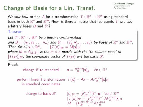
Coordinate ChangeDiagonalizationApplicationsChange of Basis for a Lin. Transf.
We saw how to find A for a transformation T : Rn → Rm using standardbasis in both Rn and Rm. Now: is there a matrix that represents T wrt twoarbitrary bases B and B ′?TheoremLet T : Rn → Rm be a linear transformationand B = {v1, v2, . . . , vn} and B ′ = {v′1, v′2, . . . , v′n} be bases of Rn and Rm.Then for all x ∈ Rn, [T (x)]B′ = M[x]Bwhere M = A[B,B′] is the m × n matrix with the ith column equal to[T (vi )]B′ , the coordinate vector of T (vi ) wrt the basis B ′.
Proof:change B to standard x = Pn×n
B [x]B ∀x ∈ Rn
↓perform linear transformation T (x) = Ax = APn×n
B [x]Bin standard coordinates
↓change to basis B ′ [u]B′ = (Pm×m
B′ )−1u ∀u ∈ Rm
[T (x)]B′ = (Pm×mB′ )−1APn×n
B [x]BM = (Pm×m
B′ )−1APn×nB 5

Coordinate ChangeDiagonalizationApplications
How is M done?
• PB = [v1 v2 . . . vn]
• APB = A[v1 v2 . . . vn] = [Av1 Av2 . . . Avn]
• Avi = T (vi ): APB = [T (v1) T (v2) . . . T (vn)]
• M = P−1B′ APB = P−1
B′ = [P−1B′ T (v1) P−1
B′ T (v2) . . . P−1B′ T (vn)]
• M = [[T (v1)]B′ [T (v2)]B′ . . . [T (vn)]B′ ]
Hence, if we change the basis from the standard basis of Rn and Rm thematrix representation of T changes
6
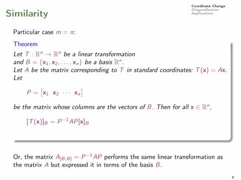
Coordinate ChangeDiagonalizationApplicationsSimilarity
Particular case m = n:
TheoremLet T : Rn → Rn be a linear transformationand B = {x1, x2, . . . , xn} be a basis Rn.Let A be the matrix corresponding to T in standard coordinates: T (x) = Ax.Let
P =[x1 x2 · · · xn
]be the matrix whose columns are the vectors of B. Then for all x ∈ Rn,
[T (x)]B = P−1AP[x]B
Or, the matrix A[B,B] = P−1AP performs the same linear transformation asthe matrix A but expressed it in terms of the basis B.
7
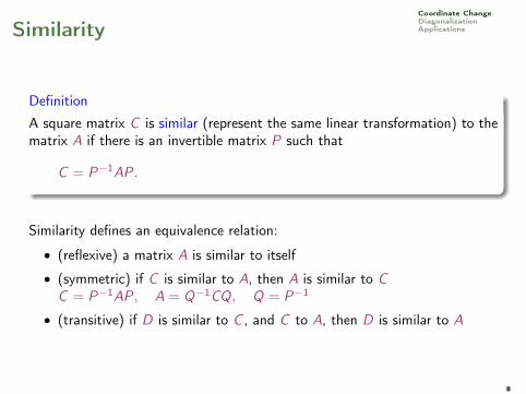
Coordinate ChangeDiagonalizationApplicationsSimilarity
Definition
A square matrix C is similar (represent the same linear transformation) to thematrix A if there is an invertible matrix P such that
C = P−1AP.
Similarity defines an equivalence relation:
• (reflexive) a matrix A is similar to itself
• (symmetric) if C is similar to A, then A is similar to CC = P−1AP, A = Q−1CQ, Q = P−1
• (transitive) if D is similar to C , and C to A, then D is similar to A
8

Example
2−2
1
−1
x
y
2−2
1
−1
x
y
• x2 + y2 = 1 circle in standard form
• x2 + 4y2 = 4 ellipse in standard form
• 5x2 + 5y2 − 6xy = 2 ??? Try rotating π/4 anticlockwise
AT =
[cos θ − sin θsin θ cos θ
]=
[1√2− 1√
21√2
1√2
]= P
v = P[v]B ⇐⇒[xy
]=
[1√2− 1√
21√2
1√2
] [XY
]X 2 + 4Y 2 = 1
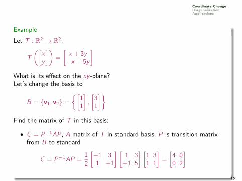
Coordinate ChangeDiagonalizationApplications
Example
Let T : R2 → R2:
T([
xy
])=
[x + 3y−x + 5y
]What is its effect on the xy -plane?Let’s change the basis to
B = {v1, v2} ={[
11
],
[31
]}Find the matrix of T in this basis:
• C = P−1AP, A matrix of T in standard basis, P is transition matrixfrom B to standard
C = P−1AP =12
[−1 31 −1
] [1 3−1 5
] [1 31 1
]=
[4 00 2
]10

Coordinate ChangeDiagonalizationApplications
Example (cntd)
• the B coordinates of the B basis vectors are
[v1]B =
[10
]B, [v2]B =
[01
]B
• so in B coordinates T is a stretch in the direction v1 by 4 and in dir. v2by 2:
[T (v1)]B =
[4 00 2
] [10
]B=
[40
]B= 4[v1]B
• The effect of T is however the same no matter what basis, only thematrices change! So also in the standard coordinates we must have:
Av1 = 4v1 Av2 = 2v2
11

Coordinate ChangeDiagonalizationApplicationsResume
• Matrix representation of a transformation with respect to two given basis
• Similarity of square matrices
12

Coordinate ChangeDiagonalizationApplicationsOutline
1. More on Coordinate Change
2. Diagonalization
3. Applications
13
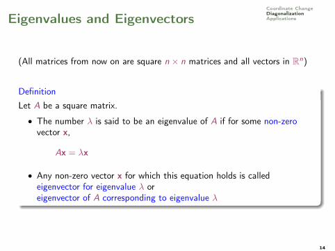
Coordinate ChangeDiagonalizationApplicationsEigenvalues and Eigenvectors
(All matrices from now on are square n × n matrices and all vectors in Rn)
DefinitionLet A be a square matrix.
• The number λ is said to be an eigenvalue of A if for some non-zerovector x,
Ax = λx
• Any non-zero vector x for which this equation holds is calledeigenvector for eigenvalue λ oreigenvector of A corresponding to eigenvalue λ
14

Coordinate ChangeDiagonalizationApplicationsFinding Eigenvalues
• Determine solutions to the matrix equation Ax = λx
• Let’s put it in standard form, using λx = λIx:
(A− λI )x = 0
• Bx = 0 has solutions other than x = 0 precisely when det(B) = 0.
• hence we want det(A− λI ) = 0:
Definition (Charachterisitc polynomial)
The polynomial |A− λI | is called the characteristic polynomial of A, andthe equation |A− λI | = 0 is called the characteristic equation of A.
15

Coordinate ChangeDiagonalizationApplications
Example
A =
[7 −152 −4
]
A− λI =[7 −152 −4
]− λ
[1 00 1
]=
[7− λ −152 −4− λ
]The characteristic polynomial is
|A− λI | =∣∣∣∣7− λ −15
2 −4− λ
∣∣∣∣= (7− λ)(−4− λ) + 30= λ2 − 3λ+ 2
The characteristic equation is
λ2 − 3λ+ 2 = (λ− 1)(λ− 2) = 0
hence 1 and 2 are the only eigenvalues of A16

Coordinate ChangeDiagonalizationApplicationsFinding Eigenvectors
• Find non-trivial solution to (A− λI )x = 0 corresponding to λ
• zero vectors are not eigenvectors!
Example
A =
[7 −152 −4
]Eigenvector for λ = 1:
A− I =[6 −152 −5
]→ RREF· · · →
[1 − 5
20 0
]v = t
[52
], t ∈ R
Eigenvector for λ = 2:
A− 2I =[5 −152 −6
]→ RREF· · · →
[1 −30 0
]v = t
[31
], t ∈ R
17

Coordinate ChangeDiagonalizationApplications
Example
A =
4 0 40 4 44 4 8
The characteristic equation is
|A− λI | =
∣∣∣∣∣∣4− λ 0 4
0 4− λ 44 4 8− λ
∣∣∣∣∣∣= (4− λ)((−4− λ)(8− λ)− 16) + 4(−4(4− λ))= (4− λ)((−4− λ)(8− λ)− 16)− 16(4− λ)= (4− λ)((−4− λ)(8− λ)− 16− 16)= (4− λ)λ(λ− 12)
hence the eigenvalues are 4, 0, 12.Eigenvector for λ = 4, solve (A− 4I )x = 0:
A−4I =
4− 4 0 40 4− 4 44 4 8− 4
→ RREF· · · →
1 1 00 0 10 0 0
v = t
−110
, t ∈ R
18
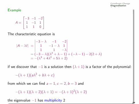
Coordinate ChangeDiagonalizationApplications
Example
A =
−3 −1 −21 −1 11 1 0
The characteristic equation is
|A− λI | =
∣∣∣∣∣∣−3− λ −1 −2
1 −1− λ 11 1 −λ
∣∣∣∣∣∣= (−3− λ)(λ2 + λ− 1) + (−λ− 1)− 2(2 + λ)= −(λ3 + 4λ2 + 5λ+ 2)
if we discover that −1 is a solution then (λ+ 1) is a factor of the polynomial:
−(λ+ 1)(aλ2 + bλ+ c)
from which we can find a = 1, c = 2, b = 3 and
−(λ+ 1)(λ+ 2)(λ+ 1) = −(λ+ 1)2(λ+ 2)
the eigenvalue −1 has multiplicity 219
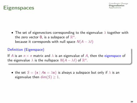
Coordinate ChangeDiagonalizationApplicationsEigenspaces
• The set of eigenvectors corresponding to the eigenvalue λ together withthe zero vector 0, is a subspace of Rn.because it corresponds with null space N(A− λI )
Definition (Eigenspace)
If A is an n × n matrix and λ is an eigenvalue of A, then the eigenspace ofthe eigenvalue λ is the nullspace N(A− λI ) of Rn.
• the set S = {x | Ax = λx} is always a subspace but only if λ is aneigenvalue then dim(S) ≥ 1.
20
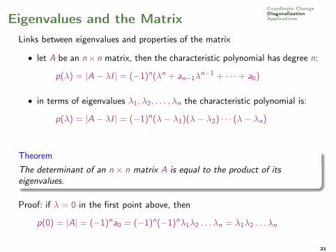
Coordinate ChangeDiagonalizationApplicationsEigenvalues and the Matrix
Links between eigenvalues and properties of the matrix
• let A be an n×n matrix, then the characteristic polynomial has degree n:
p(λ) = |A− λI | = (−1)n(λn + an−1λn−1 + · · ·+ a0)
• in terms of eigenvalues λ1, λ2, . . . , λn the characteristic polynomial is:
p(λ) = |A− λI | = (−1)n(λ− λ1)(λ− λ2) · · · (λ− λn)
TheoremThe determinant of an n × n matrix A is equal to the product of itseigenvalues.
Proof: if λ = 0 in the first point above, then
p(0) = |A| = (−1)na0 = (−1)n(−1)nλ1λ2 . . . λn = λ1λ2 . . . λn
21
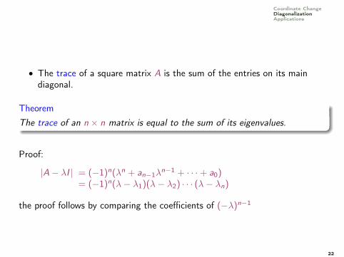
Coordinate ChangeDiagonalizationApplications
• The trace of a square matrix A is the sum of the entries on its maindiagonal.
TheoremThe trace of an n × n matrix is equal to the sum of its eigenvalues.
Proof:
|A− λI | = (−1)n(λn + an−1λn−1 + · · ·+ a0)
= (−1)n(λ− λ1)(λ− λ2) · · · (λ− λn)
the proof follows by comparing the coefficients of (−λ)n−1
22

Coordinate ChangeDiagonalizationApplicationsDiagonalization
Recall: Square matrices are similar if there is an invertible matrix P such thatP−1AP = M.
Definition (Diagonalizable matrix)
The matrix A is diagonalizable if it is similar to a diagonal matrix; that is,if there is a diagonal matrix D and an invertible matrix P such thatP−1AP = D
Example
A =
[7 −152 −4
]
P =
[5 32 1
]P−1 =
[−1 32 −5
]
P−1AP = D =
[1 00 2
]How was such a matrix P found?
When a matrix is diagonalizable?
23

Coordinate ChangeDiagonalizationApplicationsGeneral Method
• Let’s assume A is diagonalizable, then P−1AP = D where
D = diag(λ1, λ2, . . . , λn) =
λ1 0 · · · 00 λ2 · · · 0
0 0. . . 0
0 0 · · · λn
• AP = PD
AP = A[v1 · · · vn
]=[Av1 · · · Avn
]
PD =[v1 · · · vn
]λ1 0 · · · 00 λ2 · · · 0
0 0. . . 0
0 0 · · · λn
=[λ1v1 · · · λnvn
]
• Hence: Av1 = λ1v1, Av2 = λ2v2, · · · Avn = λnvn24
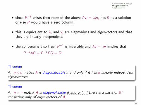
Coordinate ChangeDiagonalizationApplications
• since P−1 exists then none of the above Avi = λivi has 0 as a solutionor else P would have a zero column.
• this is equivalent to λi and vi are eigenvalues and eigenvectors and thatthey are linearly independent.
• the converse is also true: P−1 is invertible and Av = λv implies that
P−1AP = P−1PD = D
TheoremAn n× n matrix A is diagonalizable if and only if it has n linearly independenteigenvectors.
TheoremAn n × n matrix A is diagonalizable if and only if there is a basis of Rn
consisting only of eigenvectors of A.
25
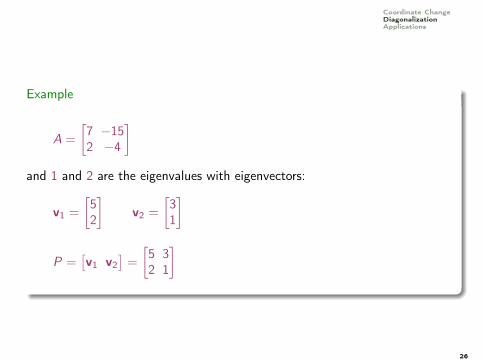
Coordinate ChangeDiagonalizationApplications
Example
A =
[7 −152 −4
]and 1 and 2 are the eigenvalues with eigenvectors:
v1 =
[52
]v2 =
[31
]
P =[v1 v2
]=
[5 32 1
]
26
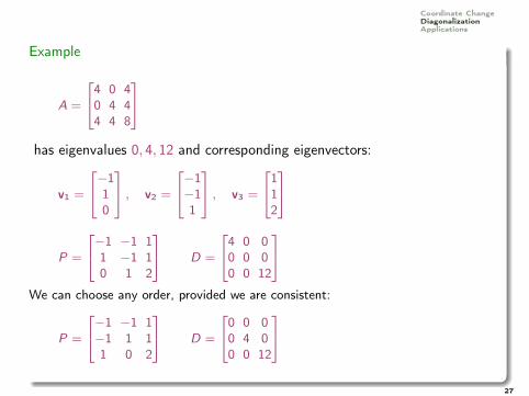
Coordinate ChangeDiagonalizationApplications
Example
A =
4 0 40 4 44 4 8
has eigenvalues 0, 4, 12 and corresponding eigenvectors:
v1 =
−110
, v2 =
−1−11
, v3 =
112
P =
−1 −1 11 −1 10 1 2
D =
4 0 00 0 00 0 12
We can choose any order, provided we are consistent:
P =
−1 −1 1−1 1 11 0 2
D =
0 0 00 4 00 0 12
27
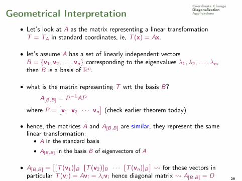
Coordinate ChangeDiagonalizationApplicationsGeometrical Interpretation
• Let’s look at A as the matrix representing a linear transformationT = TA in standard coordinates, ie, T (x) = Ax.
• let’s assume A has a set of linearly independent vectorsB = {v1, v2, . . . , vn} corresponding to the eigenvalues λ1, λ2, . . . , λn,then B is a basis of Rn.
• what is the matrix representing T wrt the basis B?
A[B,B] = P−1AP
where P =[v1 v2 · · · vn
](check earlier theorem today)
• hence, the matrices A and A[B,B] are similar, they represent the samelinear transformation:
• A in the standard basis
• A[B,B] in the basis B of eigenvectors of A
• A[B,B] =[[T (v1)]B [T (v2)]B · · · [T (vn)]B
] for those vectors in
particular T (vi ) = Avi = λivi hence diagonal matrix A[B,B] = D 28
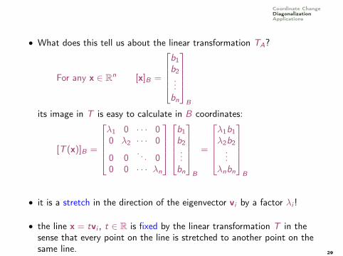
Coordinate ChangeDiagonalizationApplications
• What does this tell us about the linear transformation TA?
For any x ∈ Rn [x]B =
b1b2...bn
B
its image in T is easy to calculate in B coordinates:
[T (x)]B =
λ1 0 · · · 00 λ2 · · · 0
0 0. . . 0
0 0 · · · λn
b1b2...bn
B
=
λ1b1λ2b2...
λnbn
B
• it is a stretch in the direction of the eigenvector vi by a factor λi !
• the line x = tvi , t ∈ R is fixed by the linear transformation T in thesense that every point on the line is stretched to another point on thesame line. 29
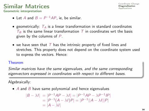
Coordinate ChangeDiagonalizationApplicationsSimilar Matrices
Geometric interpretation
• Let A and B = P−1AP, ie, be similar.
• geometrically: TA is a linear transformation in standard coordinatesTB is the same linear transformation T in coordinates wrt the basisgiven by the columns of P.
• we have seen that T has the intrinsic property of fixed lines andstretches. This property does not depend on the coordinate system usedto express the vectors. Hence:
TheoremSimilar matrices have the same eigenvalues, and the same correspondingeigenvectors expressed in coordinates with respect to different bases.
Algebraically:
• A and B have same polynomial and hence eigenvalues
|B − λI | = |P−1AP − λI | = |P−1AP − λP−1IP|= |P−1(A− λI )P| = |P−1||A− λI ||P|= |A− λI |
30

Coordinate ChangeDiagonalizationApplications
• P transition matrix from the basis S to the standard coords to coords
v = P[v]S [v]S = P−1v
• Using Av = λv:
B[v]S = P−1AP[v]S= P−1Av= P−1λv= λP−1v= λ[v]S
hence [v]S is eigenvector of B corresponding to eigenvalue λ
31

Coordinate ChangeDiagonalizationApplicationsDiagonalizable matrices
Example
A =
[4 1−1 2
]has characteristic polynomial λ2 − 6λ+ 9 = (λ− 3)2.The eigenvectors are:[
1 1−1 −1
] [x1x2
]=
[00
]
v = [−1, 1]T
hence any two eigenvectors are scalar multiple of each others and are linearlydependent.
The matrix A is therefore not diagonalizable.
32
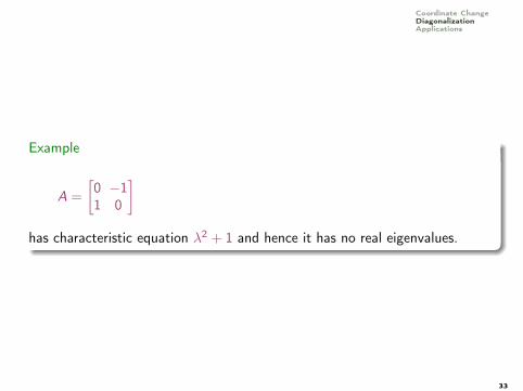
Coordinate ChangeDiagonalizationApplications
Example
A =
[0 −11 0
]has characteristic equation λ2 + 1 and hence it has no real eigenvalues.
33

Coordinate ChangeDiagonalizationApplications
Theorem
If an n× n matrix A has n different eigenvalues then (it has a set of n linearlyindependent eigenvectors) is diagonalizable.
• Proof by contradiction
• n lin indep. is necessary condition but n different eigenvalues not.
Example
A =
3 −1 10 2 01 −1 3
the characteristic polynomial is −(λ− 2)2(λ− 4). Hence 2 has multiplicity 2.Can we find two corresponding linearly independent vectors?
34

Coordinate ChangeDiagonalizationApplications
Example (cntd)
(A− 2I ) =
1 −1 10 0 01 −1 1
→ RREF· · · →
1 −1 10 0 00 0 0
x = s
110
+ t
−101
= sv1 + tv2 s, t ∈ R
the two vectors are lin. indep.
(A− 4I ) =
−1 −1 10 −2 01 −1 −1
→ RREF· · · →
1 0 −10 1 00 0 0
v3 =
101
P =
1 1 −10 1 01 0 1
P−1AP =
4 0 00 2 00 0 2
35
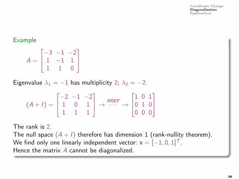
Coordinate ChangeDiagonalizationApplications
Example
A =
−3 −1 −21 −1 11 1 0
Eigenvalue λ1 = −1 has multiplicity 2; λ2 = −2.
(A+ I ) =
−2 −1 −21 0 11 1 1
→ RREF· · · →
1 0 10 1 00 0 0
The rank is 2.The null space (A+ I ) therefore has dimension 1 (rank-nullity theorem).We find only one linearly independent vector: x = [−1, 0, 1]T .Hence the matrix A cannot be diagonalized.
36
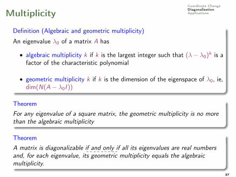
Coordinate ChangeDiagonalizationApplicationsMultiplicity
Definition (Algebraic and geometric multiplicity)
An eigenvalue λ0 of a matrix A has
• algebraic multiplicity k if k is the largest integer such that (λ− λ0)k is a
factor of the characteristic polynomial
• geometric multiplicity k if k is the dimension of the eigenspace of λ0, ie,dim(N(A− λ0I ))
TheoremFor any eigenvalue of a square matrix, the geometric multiplicity is no morethan the algebraic multiplicity
TheoremA matrix is diagonalizable if and only if all its eigenvalues are real numbersand, for each eigenvalue, its geometric multiplicity equals the algebraicmultiplicity.
37
Coordinate ChangeDiagonalizationApplicationsSummary
• Characteristic polynomial and characteristic equation of a matrix
• eigenvalues, eigenvectors, diagonalization
• finding eigenvalues and eigenvectors
• eigenspace
• eigenvalues are related to determinant and trace of a matrix
• diagonalize a diagonalizable matrix
• conditions for digonalizability
• diagonalization as a change of basis, similarity
• geometric effect of linear transformation via diagonalization38

Coordinate ChangeDiagonalizationApplicationsOutline
1. More on Coordinate Change
2. Diagonalization
3. Applications
39
Coordinate ChangeDiagonalizationApplicationsUses of Diagonalization
• find powers of matrices
• solving systems of simultaneous linear difference equations
• Markov chains
• systems of differential equations
40

Coordinate ChangeDiagonalizationApplicationsPowers of Matrices
An = AAA · · ·A︸ ︷︷ ︸n times
If we can write: P−1AP = D then A = PDP−1
An = AAA · · ·A︸ ︷︷ ︸n times
= (PDP−1)(PDP−1)(PDP−1) · · · (PDP−1)︸ ︷︷ ︸n times
= PD(P−1P)D(P−1P)D(P−1P) · · ·DP−1
= P DDD · · ·D︸ ︷︷ ︸n times
P−1
= PDnP−1
then closed formula to calculate the power of a matrix.
41
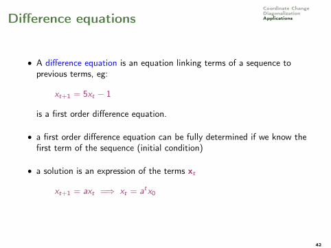
Coordinate ChangeDiagonalizationApplicationsDifference equations
• A difference equation is an equation linking terms of a sequence toprevious terms, eg:
xt+1 = 5xt − 1
is a first order difference equation.
• a first order difference equation can be fully determined if we know thefirst term of the sequence (initial condition)
• a solution is an expression of the terms xt
xt+1 = axt =⇒ xt = atx0
42
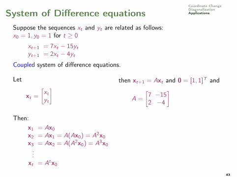
Coordinate ChangeDiagonalizationApplicationsSystem of Difference equations
Suppose the sequences xt and yt are related as follows:x0 = 1, y0 = 1 for t ≥ 0
xt+1 = 7xt − 15ytyt+1 = 2xt − 4yt
Coupled system of difference equations.
Let
xt =
[xtyt
] then xt+1 = Axt and 0 = [1, 1]T and
A =
[7 −152 −4
]Then:
x1 = Ax0x2 = Ax1 = A(Ax0) = A2x0x3 = Ax2 = A(A2x0) = A3x0...
xt = Atx0
43
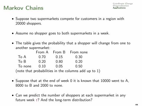
Coordinate ChangeDiagonalizationApplicationsMarkov Chains
• Suppose two supermarkets compete for customers in a region with20000 shoppers.
• Assume no shopper goes to both supermarkets in a week.
• The table gives the probability that a shopper will change from one toanother supermarket:
From A From B From noneTo A 0.70 0.15 0.30To B 0.20 0.80 0.20To none 0.10 0.05 0.50
(note that probabilities in the columns add up to 1)
• Suppose that at the end of week 0 it is known that 10000 went to A,8000 to B and 2000 to none.
• Can we predict the number of shoppers at each supermarket in anyfuture week t? And the long-term distribution?
44
Coordinate ChangeDiagonalizationApplications
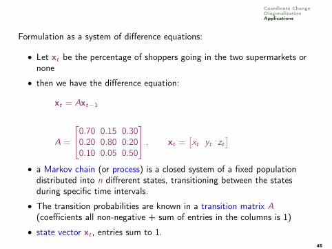
Formulation as a system of difference equations:
• Let xt be the percentage of shoppers going in the two supermarkets ornone
• then we have the difference equation:
xt = Axt−1
A =
0.70 0.15 0.300.20 0.80 0.200.10 0.05 0.50
, xt =[xt yt zt
]• a Markov chain (or process) is a closed system of a fixed populationdistributed into n diffrerent states, transitioning between the statesduring specific time intervals.
• The transition probabilities are known in a transition matrix A(coefficients all non-negative + sum of entries in the columns is 1)
• state vector xt , entries sum to 1.45
Coordinate ChangeDiagonalizationApplications
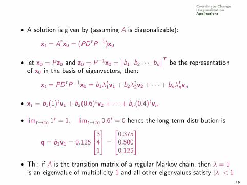
• A solution is given by (assuming A is diagonalizable):
xt = Atx0 = (PDtP−1)x0
• let x0 = Pz0 and z0 = P−1x0 =[b1 b2 · · · bn
]T be the representationof x0 in the basis of eigenvectors, then:
xt = PDtP−1x0 = b1λt1v1 + b2λ
t2v2 + · · ·+ bnλ
tnvn
• xt = b1(1)tv1 + b2(0.6)tv2 + · · ·+ bn(0.4)tvn
• limt→∞ 1t = 1, limt→∞ 0.6t = 0 hence the long-term distribution is
q = b1v1 = 0.125
341
=
0.3750.5000.125
• Th.: if A is the transition matrix of a regular Markov chain, then λ = 1is an eigenvalue of multiplicity 1 and all other eigenvalues satisfy |λ| < 1
46