Divergent Series: A Numeristic Approach - Kevin Carmody

DIVERGENT SERIES

A NUMERISTIC APPROACH

Kevin Carmody1000 University Manor Drive, Apt. 34

Fairfield, Iowa [email protected]

Eighth edition5 June 2017

Copyright c© 2001–2017 Kevin Carmody

Eighth edition 5 June 2017Seventh edition 2 September 2016

Sixth edition 24 March 2016Fifth edition 4 March 2012

Fourth edition 7 December 2010Third edition 26 June 2008

Second edition 2003First edition 2001

CONTENTS

Summary . . . . . . . . . . . . . . . . . . . . . . . . . . . . . . . . . . . . . . . . . . . . . . . . . . . . . . . . . . . . . . . . . . . . . . . . . . . . . . . . 5

Epigraph . . . . . . . . . . . . . . . . . . . . . . . . . . . . . . . . . . . . . . . . . . . . . . . . . . . . . . . . . . . . . . . . . . . . . . . . . . . . . . . . . 6

Introduction . . . . . . . . . . . . . . . . . . . . . . . . . . . . . . . . . . . . . . . . . . . . . . . . . . . . . . . . . . . . . . . . . . . . . . . . . . . . . 7

Some results of Equation 2 . . . . . . . . . . . . . . . . . . . . . . . . . . . . . . . . . . . . . . . . . . . . . . . . . . . . . . . . . . . . . 11

Other infinite series . . . . . . . . . . . . . . . . . . . . . . . . . . . . . . . . . . . . . . . . . . . . . . . . . . . . . . . . . . . . . . . . . . . . 21

Results involving infinite products . . . . . . . . . . . . . . . . . . . . . . . . . . . . . . . . . . . . . . . . . . . . . . . . . . . . 26

Results involving divergent integrals . . . . . . . . . . . . . . . . . . . . . . . . . . . . . . . . . . . . . . . . . . . . . . . . . . 33

Infinite series have infinite values . . . . . . . . . . . . . . . . . . . . . . . . . . . . . . . . . . . . . . . . . . . . . . . . . . . . . 35

Equipoint summation . . . . . . . . . . . . . . . . . . . . . . . . . . . . . . . . . . . . . . . . . . . . . . . . . . . . . . . . . . . . . . . . . . 42

Introduction . . . . . . . . . . . . . . . . . . . . . . . . . . . . . . . . . . . . . . . . . . . . . . . . . . . . . . . . . . . . . . . . . . . . . 42

Sum of zeros . . . . . . . . . . . . . . . . . . . . . . . . . . . . . . . . . . . . . . . . . . . . . . . . . . . . . . . . . . . . . . . . . . . . 43

Sum of infinities . . . . . . . . . . . . . . . . . . . . . . . . . . . . . . . . . . . . . . . . . . . . . . . . . . . . . . . . . . . . . . . . 47

Sum of non-idempotents . . . . . . . . . . . . . . . . . . . . . . . . . . . . . . . . . . . . . . . . . . . . . . . . . . . . . . . 49

Absolute sum of units . . . . . . . . . . . . . . . . . . . . . . . . . . . . . . . . . . . . . . . . . . . . . . . . . . . . . . . . . . 51

Alternating sum of units . . . . . . . . . . . . . . . . . . . . . . . . . . . . . . . . . . . . . . . . . . . . . . . . . . . . . . . . 53

Alternating arithmetic series . . . . . . . . . . . . . . . . . . . . . . . . . . . . . . . . . . . . . . . . . . . . . . . . . . . . 55

Absolute arithmetic series . . . . . . . . . . . . . . . . . . . . . . . . . . . . . . . . . . . . . . . . . . . . . . . . . . . . . . 58

A practical application . . . . . . . . . . . . . . . . . . . . . . . . . . . . . . . . . . . . . . . . . . . . . . . . . . . . . . . . . . . . . . . . . 61

Comparison to conventional theory . . . . . . . . . . . . . . . . . . . . . . . . . . . . . . . . . . . . . . . . . . . . . . . . . . . 64

Three approaches . . . . . . . . . . . . . . . . . . . . . . . . . . . . . . . . . . . . . . . . . . . . . . . . . . . . . . . . . . . . . . . 64

Other approaches . . . . . . . . . . . . . . . . . . . . . . . . . . . . . . . . . . . . . . . . . . . . . . . . . . . . . . . . . . . . . . . 65

Objections . . . . . . . . . . . . . . . . . . . . . . . . . . . . . . . . . . . . . . . . . . . . . . . . . . . . . . . . . . . . . . . . . . . . . . . 66

The conventional theory of divergent series . . . . . . . . . . . . . . . . . . . . . . . . . . . . . . . . . . . 71

Contents 3

Methods of summation . . . . . . . . . . . . . . . . . . . . . . . . . . . . . . . . . . . . . . . . . . . . . . . . . . . . . . . . . 72

Ramanujan summation . . . . . . . . . . . . . . . . . . . . . . . . . . . . . . . . . . . . . . . . . . . . . . . . . . . . . . . . . 75

The Euler extension method of summation . . . . . . . . . . . . . . . . . . . . . . . . . . . . . . . . . . . . 80

Analytic continuation . . . . . . . . . . . . . . . . . . . . . . . . . . . . . . . . . . . . . . . . . . . . . . . . . . . . . . . . . . . 84

Summary of the numeristic approach to divergent series . . . . . . . . . . . . . . . . . . . . . . . . . . . . 86

Numeristics in general . . . . . . . . . . . . . . . . . . . . . . . . . . . . . . . . . . . . . . . . . . . . . . . . . . . . . . . . . . . . . . . . . 87

Appendix: Mathematicians’ opinions about divergent series . . . . . . . . . . . . . . . . . . . . . . . . . 88

Acknowledgment . . . . . . . . . . . . . . . . . . . . . . . . . . . . . . . . . . . . . . . . . . . . . . . . . . . . . . . . . . . . . . . . . . . . . . 94

References . . . . . . . . . . . . . . . . . . . . . . . . . . . . . . . . . . . . . . . . . . . . . . . . . . . . . . . . . . . . . . . . . . . . . . . . . . . . . . 95

4 Contents

SUMMARY

Infinite divergent series can generate some striking results but have been contro-versial for centuries. The standard approaches of limits and methods of summation havedrawbacks which do not account for the full range of behavior of these series. A simplerapproach using numeristics is developed, which better accounts for divergent series andtheir sums. Numeristics is introduced in a separate monograph.

The modern theory of divergent series can be said to begin with Euler, whose basictechnique we call the Euler extension method. The numeristic approach starts with thismethod and has two basic aspects:

1. Recursion, which is the Euler extension method coupled with the under-standing that most infinite series have at least two values, one finite and oneinfinite. For example, using recursion, we establish that 1 + 2 + 4 + 8 + . . . ={−1,∞}.

2. Equipoint summation, which uses equipoint analysis, introduced in a sep-arate monograph.

Equipoint analysis uses multiple levels of sensitivity to unfold real and complexnumbers to multilevel numbers, functions, and relations. Equipoint summation usesthese multiple levels to unfold the terms of an infinite series, which shows that the sumof a divergent series may depend on the mode of unfolding. For instance, 1−1+1−1+ . . .may have the value ∞, 1

2 , an arbitrary finite number, 1, or 0, depending on the mode ofunfolding the terms.

Various objections to numeristic approach are addressed. It is shown that the nu-meristic approach enables the use of algebraic properties that are commonly used to han-dle finite expressions but that conventional theory claims do not hold for infinite series.This simplifies the handling of infinite series, including divergent series, while providinga consistent and simple approach that handles a wide variety of cases.

Summary 5

[I]n the early years of this century [the 20th] the subject, while in no way mysticalor unrigorous, was regarded as sensational, and about the present title [Divergent Series],now colourless, there hung an aroma of paradox and audacity.—J. E. Littlewood in hispreface to [H]

6 Epigraph

INTRODUCTION

In this monograph, we will see that we can find finite sums for infinite divergentseries. Surprisingly, we find that it is controversial among mathematicians as to whetherthese series even have sums. We will examine this topic in some detail, and we willdevelop an approach which enables us to better appreciate these series and the surprisingnature of the infinite which they show.

This approach is an application of numeristics, a number based foundational the-ory. Numeristics is introduced in [CN]; the present monograph is a sequel.

A finite geometric series

n∑k=m

ak = am + am+1 + am+2 + am+3 + . . . + an

can easily be summed by through a recurrence formula. We let x be the sum:

x =n∑

k=m

ak = am + am+1 + am+2 + am+3 + . . . + an,

and then we multiply both sides by a:

xa = am+1 + am+2 + am+3 + am+4 + . . . + an+1,

and then we observe that xa + am = x + an+1. We therefore have x − xa = am − an+1, whichyields

x =am − an+1

1 − a ,

the well-known result

n∑k=m

ak = am + am+1 + am+2 + am+3 + . . . + an =am − an+1

1 − a . (1)

An infinite geometric series can also be summed in this way. If we have

∞∑k=m

ak = am + am+1 + am+2 + am+3 + . . . ,

Introduction 7

then again we set

x =∞∑k=m

ak = am + am+1 + am+2 + am+3 + . . . ,

again multiply both sides by a,

xa = am+1 + am+2 + am+3 + am+4 + . . . ,

and observe that xa + am = x, yielding x − xa = am, or

x =am

1 − a,

and another well-known result

∞∑k=m

ak = am + am+1 + am+2 + am+3 + . . . =am

1 − a. (2)

If m = 0, that is, if the first term is 1, then this result becomes

∞∑k=0

ak = 1 + a + a2 + a3 + . . . =1

1 − a. (3)

For example, if a = 12 andm = 1, then the infinite geometric series is 1

2+14+

18+

116+. . ..

Equation 2 says that this sum is 1/21−1/2 = 1, that is

∞∑k=1

12k

=12+

14+

18+

116

+ . . . = 1. (4)

Figure 1 shows a visualization of this sum, and the formula seems to agree with

what we observe in such a diagram.

8 Introduction

FIG. 1: Diagram of 1/2 + 1/4 + 1/8 + 1/16 + . . . = 1

It has long been noticed that, when derived this way, Equation 2 seems to hold foralmost any a. For example, if a = 2, we could conclude that

∞∑k=0

2k = 1 + 2 + 4 + 8 + . . . = −1. (5)

This may come as an even bigger surprise than Equation 4. Naturally, it might bewondered how Equation 5could be true. The intermediate results, 1, 1+2 = 3, 1+2+4 = 7,1 + 2 + 4 + 8 = 15, etc., known as partial sums, grow without limit and are always positive,whereas in Equation 4, the partial sums 1, 1 + 1

2 = 32 , 1 + 1

2 + 14 = 7

4 , 1 + 12 + 1

4 + 18 = 15

8 , etc.,get progressively closer to 2 but never exceed it.

Infinite series such as the one in Equation 4, in which the partial sums approacha fixed number, are known as convergent, while those that do not, such as the one inEquation 5, are known as divergent.

There are two general points of view on convergent and divergent infinite series.The conventional point of view is that divergent series are meaningless and have no sum,and only convergent series have a sum. In this view, the number that the partial sumsconverge to, called the limit, is considered the sum of the infinite series.

The alternative point of view is that divergent series are not automatically mean-ingless but may have a sum. Following this point of view, a theory of divergent series hasbeen developed. This theory is generally consistent and even has a number of applica-tions. References [Bo, F, H, Mo, Sm, Sz] are some of the important standard works of thistheory, with [H] often being regarded as the most important.

In this monograph, we will explore some of the results of this theory. We willuse a new approach which resolves some longstanding problems. This approach is an

Introduction 9

application of numeristics [CN] and equipoint analysis [CE], which include an extension ofarithmetic that allows us to include any values of a, m, and n in Equation 1.

The numeristic approach uses two basic techniques:

1. Recursion, presented in the first few chapters, starting with Some results ofEquation 2.

2. Equipoint summation, an application of equipoint analysis, presented inthe Equipoint summation chapter.

Equipoint analysis includes a system of calculus which is simpler than the con-ventional system, but for infinite series, it adds a level of complexity which is not alwaysnecessary, so we save it for relatively difficult cases.

10 Introduction

SOME RESULTS OF EQUATION 2

In this chapter we examine some straightforward results of Equation 2. Subtlerpoints of the theory are examined in subsequent chapters.

0.999 . . . = 1. (6)

PROOF. This is a convergent series which we mention for completeness. 0.999 . . . =9(0.1+0.01+0.001+0.0001 . . .) = 9(10−1+10−2+10−3+10−4+. . .) = 9(0.11+0.12+0.13+0.14+. . .) =9∑∞

k=1 .01k == 9( 0.11−0.1) = 9( 0.1

0.9) = 9( 19) = 1. �

. . . 999 = −1. (7)

PROOF. By the notation . . . 999 we mean an infinite series of digits going out to theleft, just as the notation 0.999 . . . means an infinite series of digits going out to the right.Then . . . 999 = 9(1 + 10 + 100 + 1000 + . . .) = 9(100 + 101 + 102 + 103 + . . .) = 9

∑∞k=0 10k =

9( 11−10) = 9(− 1

9) = −1. �

Infinite left decimals of this type are explored in further detail in [CR].

∞∑k=−∞

ak = . . . + am−3 + am−2 + am−1 + am + am+1 + am+2 + am+3 + . . . = 0,

a 6= 1. (8)

PROOF. We have . . .+am−3 +am−2 +am−1 +am +am+1 +am+2 +am+3 + . . . = (am +am+1 +

am+2+am+3+ . . .)+(. . .+am−1+am−2+am−3+am−4+ . . .) = (am+am+1+am+2+am+3+ . . .)+(. . .+

(a−1)1−m+(a−1)2−m+(a−1)3−m+(a−1)4−m+. . .) = (am+am+1+am+2+am+3+. . .)+(. . .+(a−1)1−m+

(a−1)2−m + (a−1)3−m + (a−1)4−m + . . .) = am

1−a +am−1

1−a−1 = am

1−a +a am−1

a(1−a−1) =am

1−a +am

a−1 = am

1−a −am

1−a = 0.

Some results of Equation 2 11

Alternatively, if x = . . . + am−3 + am−2 + am−1 + am + am+1 + am+2 + am+3 + . . ., then

xa = . . .+am−2 +am−1 +am +amm + 1+am+2 +am+3 +am+4 + . . . = x, so 0 = x−xa = x(1−a).Then x must be 0, unless a = 1. �

. . . 999.999 . . . = 0. (9)

PROOF. We have . . . 999.999 . . . = 9(. . .+1000+100+10+1+0.1+0.01+0.001+ . . .) =9(. . . + 103 + 102 + 101 + 100 + 10−1 + 10−2 + 10−3 + . . .) = 9

∑∞k=−∞ 10k = 9(0) = 0. �

∞∑k=0

ekix = 1 + eix + e2ix + . . . =1 + i cot x2

2. (10)

PROOF. ekix = (eix)k , so 1 + eix + e2ix + . . . = 11−eix = 1

2 + i2

(2i

eix−1 − 1)= 1

2 + i2 cot x

2 . �

∞∑k=0

(−1)kekix = 1 − eix + e2ix − . . . =1 − i tan x

2

2. (11)

PROOF. In Equation 10, substitute x with x + π . �

∞∑k=1

[ekix

k− (−1)k

1k

]= eix +

e2ix

2+e3ix

3+ . . . + 1 − 1

2+

13− . . .

= − ln sinx

2+ i

π − x2

. (12)

PROOF. Integrate Equation 10 from π to x to obtain x − ieix − i e2ix

2 − ie3ix

3 − . . . − i +i2 −

i3 + . . . = x−π

2 + i ln sin x2 . �

∞∑k=0

(−1)ke(2k+1)ix = eix − e3ix + e5ix − . . . = secx2

. (13)

PROOF. eix − e3ix + e5ix − . . . = eix

1+e2ix = 12 secx. �

12 Some results of Equation 2

∞∑k=1

coskx = cosx + cos 2x + cos 3x + . . . = −12. (14)

PROOF. From Equation 10, cosx+ cos 2x+ . . . = Re(1 + eix + e2ix + . . .

)− 1 = 1

2 − 1 =− 1

2 . �

∞∑k=1

sinkxk

= sinx +sin 2x

2+

sin 3x3

+ . . . =π − x

2. (15)

PROOF. Integrate Equation 14 from π to x, or take the imaginary part of Equation12. �

∞∑k=1

sinkx = sinx + sin 2x + sin 3x + . . . =cot x2

2. (16)

PROOF. Take the imaginary part of Equation 10. �

∞∑k=1

[−coskx

k+ (−1)k

1k

]= − cosx − cos 2x

2− cos 3x

3+ . . . − 1 +

12− 1

3− . . .

= ln sinx

2. (17)

PROOF. Integrate Equation 16 from π to x, or take the real part of Equation 12. �

∞∑k=1

(−1)k+1 coskx = cosx − cos 2x + cos 3x − . . . = 12. (18)

PROOF. Starting with Equation 14, we replace x with x + π . Then cosnx remainsunchanged when n is even, because we are adding 2mπ to x, where n = 2m and m isan integer. But when when n is odd, then n = 2m + 1, and we are adding 2mπ + π tox, and so cosnx becomes − cosnx. This yields − cosx + cos 2x − cos 3x + . . . = − 1

2 , orcosx − cos 2x + cos 3x − . . . = 1

2 .

Alternatively, take the real part of Equation 11 and subtract 1. �


∞∑k=1

(−1)k+1 sinkxk

= sinx − sin 2x2

+cos 3x

3− . . . = x

2. (19)

PROOF. Integrate Equation 18 from 0 to x. �

∞∑k=0

(−1)k1

2k + 1= 1 − 1

3+

15− . . . = π

4. (20)

PROOF. Evaluate Equation 19 at x = π2 , or evaluate Equation 15 at x = π

2 or x = 3π2 .

�

This is a convergent series called the Gregory equation and is usually derived fromthe power series of tan−1x. While it can be used to approximate π , it is not very useful forthis purpose, since it converges very slowly.

∞∑k=1

(−1)k+1 sinkx = sinx − sin 2x + sin 3x − . . . =tan x

2

2. (21)

PROOF. We start with Equation 16 and use the same substitution, replacing x withx + π . Then sinnx remains unchanged for n even and becomes − sinnx for n odd. Inaddition, cot x

2 becomes cot(x2 + π

2

)= − tan x

2 .

Alternatively, take the imaginary part of Equation 11. �

∞∑k=1

xk

k= x +

x2

2+x3

3+x4

4+ . . . = − ln(1 − x) (22)

∞∑k=1

(−1)k+1xk

k= x − x

2

2+x3

3− x

4

4+ . . . = ln(1 + x) (23)

PROOF. From Equation 2, we have 1+x+x2+x3+. . . = 11−x and 1−x+x2−x3+. . . = 1

1+x .Integrating these from 0 to x gives the results, which are known as Mercator’s Series. �

∞∑k=1

(−1)k+1 1k= 1 +

12+

13+

14+ . . . =∞. (24)


PROOF. Evaluating Equation 22 for x = 1 gives the result, which is known as theharmonic series. �

∞∑k=1

(−1)k+1 1k= 1 − 1

2+

13− 1

4+ . . . = ln 2. (25)

PROOF. Evaluate Equation 23at x = 1. Alternatively, evaluate Equation 17 at x = π2 ,

which yields 12 −

14 + 1

6 − . . . − 1 + 12 −

13 − . . . = −

12

(1 − 1

2 + 13 − . . .

)= ln 1√

2. �

∞∑k=1

2k

k=

21+

42+

83+

164+ . . . = (2Z + 1)πi. (26)

(2Z + 1)πi is numeristic class notation for all (2k + 1)πi where k is an integer.

PROOF. Evaluate Equation 22 for x = 2 and use the fact that ln(−1) = (2Z + 1)πi. �

This result may come as an even bigger surprise than Equation 5. However, thatthe infinite sum of real numbers can be complex is simply an extension of the principleby which the infinite sum of positive numbers can be negative.

∞∑k=0

(−1)k cos(2k + 1)x = cosx − cos 3x + cos 5x − . . . = secx2

. (27)

PROOF. From Equation 13, cosx − cos 3x + cos 5x − . . . = Re(eix − e3ix + e5ix − . . .) =12 secx. �

∞∑k=0

(−1)k sin(2k + 1)x = sinx − sin 3x + sin 5x + . . . = 0. (28)

PROOF. From Equation 13, sinx− sin 3x+ sin 5x+ . . . = Im(eix − e3ix + e5ix − . . .) = 0.�

∞∑k=0

1(2k + 1)2

= 1 +132 +

152 + . . . =

π2

8. (29)


PROOF. Integrate the negative of Equation 18 from 0 to x to obtain sinx− 12 sin 2x+

13 sin 3x − . . . = 1

2x. Integrate again from 0 to x to obtain (1− cosx)− 122 (1− cos 2x) + 1

32 (1−cos 3x) − . . . = 1

4x2. Evaluate this at x = π . �

∞∑k=1

1k2 = 1 +

122 +

132 + . . . =

π2

6. (30)

PROOF. Let y = 1+ 122 + 1

32 +. . .. Then π2

8 = 1+ 122 + 1

32 +. . . = 1+ 122 + 1

32 +. . .− 122 − 1

42 −. . . =1 + 1

22 + 132 + . . . − 1

4(1 + 122 + 1

32 + . . .) = y − 14y = 3

4y = π2

6 . �

∞∑k=1

(−1)k+1 1k2 = 1 − 1

22 +132 − . . . =

π2

12. (31)

PROOF. 1− 122 + 1

32 −. . . =(

1 + 132 + 1

52 + . . .)−(

122 + 1

42 + 182 + . . .

)=(

1 + 132 + 1

52 + . . .)−

122

(1 + 1

22 + 132 + . . .

)= π2

8 −14π2

6 = π2

12 . �

∞∑k=1

(−1)k+1k2n coskx = 12n cosx − 22n cos 2x + 32n cos 3x − . . .

= 0, n = 0, 1, 2, . . . (32)∞∑k=1

(−1)k+1k2n+1 sinkx = 12n+1 sinx − 22n+1 sin 2x + 32n+1 sin 3x − . . .

= 0, n = 0, 1, 2, . . . (33)

PROOF. Repeated differentiation, n times, of Equation 18. �

∞∑k=1

(−1)k+1k2n sinkx = 12n sinx − 22n sin 2x + 32n sin 3x − . . .

= (−1)n(d

dx

)2n tan x2

2, n = 0, 1, 2, . . . (34)


∞∑k=1

(−1)k+1k2n+1 coskx = 12n+1 cosx − 22n+1 cos 2x + 32n+1 cos 3x − . . .

= (−1)n(d

dx

)2n+1 tan x2

2, n = 0, 1, 2, . . . (35)


∞∑k=0

(−1)k(2k + 1)2n cos(2k + 1)x =

12n cosx − 32n cos 3x + 52n cos 5x − . . . = (−1)n(d

dx

)2n secx2

,

n = 0, 1, 2, . . . (36)∞∑k=0

(−1)k(2k + 1)2n+1 sin(2k + 1)x =

12n+1 sinx − 32n+1 sin 3x + 52n+1 sin 5x − . . . = (−1)n(d

dx

)2n+1 secx2

,

n = 0, 1, 2, . . . (37)


∞∑k=0

(−1)k(2k + 1)2n sin(2k + 1)x =

12n sinx − 32n sin 3x + 52n sin 5x − . . . = 0, n = 0, 1, 2, . . . (38)∞∑k=0

(−1)k(2k + 1)2n+1 cos(2k + 1)x =

12n+1 cosx − 32n+1 cos 3x + 52n+1 cos 5x − . . . = 0, n = 0, 1, 2, . . . (39)



∞∑k=1

(−1)k+1k2n = 12n − 22n + 32n − . . . = 0, n = 1, 2, 3, . . . . (40)

PROOF. Evaluate Equation 32 at x = 0. �

∞∑k=0

(−1)k(2k + 1)2n+1 = 12n+1 − 32n+1 + 52n+1 − . . . = 0, n = 0, 1, 2, . . . . (41)

PROOF. Evaluate Equation 33 at x = π2 . �

∞∑k=0

(2k + 1)2n+1 = 12n+1 + 32n+1 + 52n+1 + . . . = 0, n = 0, 1, 2, . . . . (42)

PROOF. Evaluate Equation 38 at x = π2 . �

∞∑k=0

(−1)k(2k + 1)2n = 12n − 32n + 52n − . . . = 0, n = 0, 1, 2, . . . . (43)

PROOF. Evaluate Equation 39 at x = 0. �

∞∑k=1

(−1)k+1k2n+1 = 12n+1 − 22n+1 + 32n+1 + . . .

=22n+2 − 12n + 2

B2n+2, n = 0, 1, 2, . . . . (44)

PROOF. Bk stands for the k-th Bernoulli nxumber, which occurs in the power series

tanx =∑∞

k=1(−1)k−1 22k (22k−1)(2k)! B2k x

2k−1.


To prove the above identity, we evaluate

12n+1 cosx − 22n+1 cos 2x + 32n+1 cos 3x − . . . = (−1)n(d

dx

)2n+1 12

tanx

2

for x = 0. We begin by computing the power series

12

tanx

2=

12

∞∑k=1

(−1)k−1 22k (22k − 1)

(2k)!B2k

x2k−1

22k−1=∞∑k=1

(−1)k−1 22k − 1(2k)!

B2k x2k−1.

We then differentiate this series at x = 0. We observe that

(d

dx

)n

xk = k(k − 1)(k − 2) · · · (k − n + 1) xk−n.

When x = 0, this product is nonzero only when xk−n is constant, i.e. when k = n, at which

time(

ddx

)nxk = k(k − 1)(k − 2) · · · 1 = k!. This means that all terms of the power series

vanish, except for k = n.

Therefore,(

ddx

)2n+1x2k−1 = (2n + 1)! when 2n + 1 = 2k − 1 or k = n + 1, and is zero

when k 6= n + 1. We then have

(−1)n(d

dx

)2n+1 12

tanx

2= (−1)n (−1)n+2

(22n+2 − 1

)(2n + 1)!

(2n + 2)!B2n+2

=22n+2 − 12n + 2

B2n+2. �

Hardy and other older authors state this result in a different form, because theyused an older system of indexing the Bernoulli numbers. If we let B∗k represent the old


system and Bk the new, then the relation is B2k = (−1)k−1B∗k . We then obtain the olderstatement of the result,

12n+1 − 22n+1 − 32n+1 + . . . = (−1)n22n+2 − 12n + 2

B∗n+1.

∞∑k=0

(−1)k(2k + 1)2n = 12n − 32n + 52n + . . . =12E2n, n = 0, 1, 2, . . . . (45)

PROOF. Ek stands for the k-th Euler number, which occurs in the power series

secx =∑∞

n=0(−1)k 1(2k)! E2k x

2k . To prove our identity, we evaluate

12n cosx − 32n cos 2x + 52n cos 5x − . . . = (−1)n(d

dx

)2n 12

secx

for x = 0.

As before, to differentiate the power series, we use the fact that for x = 0,(ddx

)nxk = k! when k = n, and is zero when k 6= n. We then have

(−1)n(d

dx

)2n 12

secx = (−1)n (−1)n(2n)!

2 (2n)!E2n =

12E2n. �

As with the Bernoulli numbers, there is also an older system of indexing the Eulernumbers, which leads to a different form of the result by older authors. Letting E∗k repre-

sent the old system and Ek the new, the relation is E2k = (−1)kE∗k . The older statement ofthe result is then

12n − 32n + 52n + . . . = (−1)n12E∗n.


OTHER INFINITE SERIES

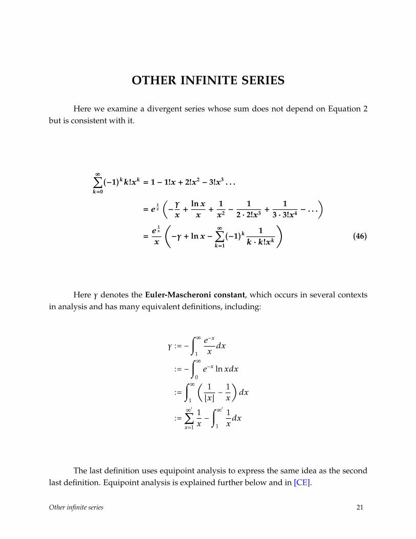
Here we examine a divergent series whose sum does not depend on Equation 2but is consistent with it.

∞∑k=0

(−1)kk!xk = 1 − 1!x + 2!x2 − 3!x3 . . .

= e1x

(−γ

x+

lnxx

+1x2 −

12 · 2!x3 +

13 · 3!x4

− . . .)

=e

1x

x

(−γ + lnx −

∞∑k=1

(−1)k1

k · k!xk

)(46)

Here γ denotes the Euler-Mascheroni constant, which occurs in several contextsin analysis and has many equivalent definitions, including:

γ := −∫∞

1

e−x

xdx

:= −∫∞

0e−x lnxdx

:=∫∞

1

(1bxc −

1x

)dx

:=∞′∑x=1

1x−∫∞′

1

1xdx

The last definition uses equipoint analysis to express the same idea as the secondlast definition. Equipoint analysis is explained further below and in [CE].

Other infinite series 21

1 2 3 4 5 6 7 8 90

1 .............................................................................................................................................................................................................................................................................

..................................................................................................................................................................................................................................

FIG. 2:γ as the area between the graphsof the sum and the integral of 1

x

PROOF. We set

f(x) := 1 − 1!x + 2!x2 − 3!x3 + . . .

g(x) := xf(x) = x − 1!x2 + 2!x3 − 3!x4 + . . .

Then

x2g ′(x) + g(x) = x2 (1! − 2!x + 3!x2 − 4!x3 + . . .)+(x − 1!x2 + 2!x3 − 3!x4 + . . .

)= x.

The equation x2g ′(x) + g(x) = x is a first order linear differential equation of theform y′(x) + P(x)y(x) = Q(x). The general solution, which we will not derive here, isy(x) = 1

I(x)

∫I(x)Q(x)dx, with the integrating factor I(x) = e

∫P(x)dx. For our specific case,

P(x) = 1x2 , Q(x) = 1

x, I(x) = e

∫dx

x2 = e−1x , and

y(x) = g(x) = e1x

∫e−

1x

xdx = e

1x

∫x0

e−1u

udu.

22 Other infinite series

Alternatively, by Equation 2,

f(x) = 1 − 1!x + 2!x2 − 3!x3 . . .

=∫∞

0e−vdv − x

∫∞0ve−vdv + x2

∫∞0v2e−vdv − x3

∫∞0v3e−vdv + . . .

=∫∞

0

e−vdv

1 + xv.

We then substitute u := x1+xv , from which we have v = 1

u− 1

xand

−e−vdv1 + xv

= −e1x

x

−xe− 1x −vdv

1 + xv

= −e1x

x

(1 + xv)e−1x −v

x

−x2dv

1 + xv

= −e1x

x

e− 1u

udu.

When v = 0, u = x, and when v =∞, u = 0, so

f(x) =g(x)x

=∫∞

0

e−vdv

1 + xv=e

1x

x

∫x0

e− 1u

udu,

the same result as above.

We now substitute w := 1u

and obtain

∫x0

e−1u

udu = −

∫ 1x

∞

e−ww

w2=∫∞

1x

e−w

wdw.


We then have

∫∞1x

e−w

wdw =

∫∞0

e−w

wdw −

∫ 1x

0

e−w

wdw

=∫∞

0

e−w

wdw + e−w lnw

∣∣∞0 −∫ 1

x

0

(1w− 1 +

w

2!− w

2

3!+ . . .

)dw

= −γ + lnw|10 − lnw|1x

0 + w|1x

0 −w2

2 · 2!

∣∣∣∣1x

0+

w3

3 · 3!

∣∣∣∣1x

0− . . .

= −γ + lnx +1x− 1

2 · 2!x2+

13 · 3!x3

− . . .

f(x) =e

1x

x

∫∞1x

e−w

wdw = e

1x

(−γ

x+

lnxx

+1x2− 1

2 · 2!x2+

13 · 3!x3

− . . .)

�

∞∑k=0

(−1)kk! = 1 − 1! + 2! − 3! . . .

= e(−γ + 2Zπi + 1 − 1

2 · 2!+

13 · 3!

− . . .)

= e

(−γ + 2Zπi −

∞∑k=1

(−1)k1

k · k!

)(47)

PROOF. Application of Equation 46 for x = 1. It has one real value and an infinitenumber of complex values. To four decimal places, its approximate value is 0.5963 +17.0795Zi. �

∞∑k=0

k! = 1 + 1! + 2! + 3! . . .

=1e

(−γ + (2Z + 1)πi + 1 +

12 · 2!

+1

3 · 3!+ . . .

)=

1e

(−γ + (2Z + 1)πi +

∞∑k=1

1k · k!

)(48)

24 Other infinite series

PROOF. Application of Equation 46 for x = −1. It has no real values but an infinitenumber of complex values. To four decimal places, its approximate value is 0.2719+1.557·(2Z + 1)i. �


RESULTS INVOLVINGINFINITE PRODUCTS

We now consider various infinite products involving prime numbers. We will firstneed to know how to multiply two infinite series, and how to multiply an infinite numberof binomials.

m∑j=1

aj

( n∑k=1

bk

)= (a1 + a2 + a3 + . . . + am)(b1 + b2 + b3 + . . . + bn)

=m∑j=1

n∑k=1

ajbk = a1b1 + a1b2 + a1b3 + . . . + a1bn

+ a2b1 + a2b2 + a2b3 + . . . + a2bn

+ a3b1 + a3b2 + a3b3 + . . . + a3bn...

+ ambn + ambn + amb3 + . . . + ambn (49)

PROOF. This is the product of two series. Both series are finite, and we simplymultiply out each series. �

(∞∑m=1

am

)(∞∑n=1

bn

)= (a1 + a2 + a3 + . . .)(b1 + b2 + b3 + . . .)

=∞∑m=1

∞∑n=1

ambn = a1b1 + a1b2 + a1b3 + . . .

+ a2b1 + a2b2 + a2b3 + . . .

+ a3b1 + a3b2 + a3b3 + . . ....

26 Results involving infinite products

=∞∑

m,n=1

ambn. (50)

PROOF. This is similar to the previous equation, but with each series now infinite.�

n∏k=1

(1 + ak) = (1 + a1)(1 + a2)(1 + a3) . . . (1 + an)

= 1 +n∑k=1

bk = 1 + b1 + b2 + b3 + . . . + bn,

where

b1 =n∑t=1

at,

b2 =n∑

t,u=1t6=u

atau,

b3 =n∑

t,u,v=1t,u,v distinct

atauav,

...

bk =n∑

t1 ,...,tk=1t1 ,...,tk distinct

at1at2at3 . . . atk

=n∑


k∏j=1

atj . (51)

PROOF. This is the product of a finite number of binomials, each with a first termof 1. The number of binomials is finite, and we multiply out their product to obtain 1 plusa sum of b terms.

For the b terms, b1 is the sum of all a, b2 is the sum of the products of any twodistinct a, b3 is the sum of the products of any three distinct a, and so on. Each bk term

Results involving infinite products 27

consists of k factors from the set of the a terms, with the index of each a term beingdistinct. �

∞∏k=1

(1 + ak) = (1 + a1)(1 + a2)(1 + a3) . . .

= 1 +∞∑k=1

bk = 1 + b1 + b2 + b3 + . . . ,

where

b1 =∞∑t=1

at,

b2 =∞∑

t,u=1t6=u

atau,

b3 =n∑

t,u,v=1t,u,v distinct

atauav,

...

bk =∞∑


at1at2at3 . . . atk

=∞∑


k∏j=1

atj . (52)

PROOF. Similar to the previous equation, but with the number of binomials nowinfinite. �

∞∏p=2

pprime

p

p − 1=

21· 3

2· 5

4· 7

6· 11

10. . .


=1

∞∏p=2

pprime

(1 − 1

p

) =1(

1 − 12

) (1 − 1

3

) (1 − 1

5

) (1 − 1

7

) (1 − 1

11

). . .

=∞∑k=1

1k= 1 +

12+

13+

14+ . . . . (53)

PROOF. The products in the first and second lines are taken over all prime num-bers. The first line becomes the second line through two identities: 1

1− 1p

= p

p−1 , and 1a· 1b= 1

ab

or its extended form∏ 1

a= 1∏

a.

To see how the second line becomes the third line, we take the first two primes, 2and 3. From Equation 2, 1

1− 12= 1 + 1

2 + 14 + 1

8 + . . ., and 11− 1

3= 1 + 1

3 + 19 + 1

27 + . . ..

By Equation 49, when we multiply these two infinite series, we get 1(1− 1

2)(1− 13)

=

1 + 12 + 1

3 + 14 + 1

6 + 18 + 1

12 + . . ., where the denominators in the sum all have as their primefactors powers of 2 and 3 only.

As we continue to multiply each side by 11− 1

p

= 1 + 1p+ 1

p2 + 1p3 + . . . for successive

prime numbers p, the denominators in the sum have as their prime factors powers of theprimes up to p. When all the prime numbers have been included in the product, all theintegers are included in the denominators in the sum. �

∞∏p=2

pprime

pn

pn − 1=

2n

1n· 3n

2n· 5n

4n· 7n

6n· 11n

10n. . .

=1

∞∏p=2

pprime

(1 − 1

pn

) =1(

1 − 12n) (

1 − 13n) (

1 − 15n) (

1 − 17n) (

1 − 111n). . .

=∞∑k=1

1kn

= 1 +1

2n+

13n

+1

4n+ . . . = ζ(n),

n = . . . ,−2,−1, 0, 1, 2, . . . . (54)


PROOF. The proof is similar to the previous equation, except that now we use aconstant power of the primes instead of the primes themselves. The last equality is thedefinition of the Riemann zeta function. �

∞∏p=2

pprime

(1 + p) = (1 + 2)(1 + 3)(1 + 5)(1 + 7)(1 + 11) . . .

=∞∑k=1

k squarefree

k = 1 + 2 + 3 + 5 + 6 + 7 + 10 + . . . ,

n = . . . ,−2,−1, 0, 1, 2, . . . . (55)

PROOF. The product in the first line is taken over all prime numbers. The sumon the second line is taken over all squarefree integers, which are those which containonly single powers of prime factors, and so are not divisible by the square of any integergreater than 1.

By Equation 52, the product on the first line when multiplied out becomes 1, plusthe sum of all p, plus the sum of the products of any two distinct p, plus the sum of theproducts of any three distinct p, and so on. Since each occurrence of p can be used at mostonce in a product, each term in the sum is squarefree. �

∞∏p=2

pprime

(1 +

1p

)=(

1 +12

)(1 +

13

)(1 +

15

)(1 +

17

)(1 +

111

). . .

=∞∑k=1

k squarefree

1k= 1 +

12+

13+

15+

16+

17+

110

+ . . . ,

n = . . . ,−2,−1, 0, 1, 2, . . . . (56)

PROOF. Similar to the above equation, with p replaced by 1p. �


∞∏p=2

pprime

(1 +

1pn

)=(

1 +1

2n

)(1 +

13n

)(1 +

15n

)(1 +

17n

)(1 +

111n

). . .

=∞∑k=1

k squarefree

1kn

= 1 +1

2n+

13n

+1

5n+

16n

+1

7n+

110n

+ . . . ,

n = . . . ,−2,−1, 0, 1, 2, . . . . (57)

PROOF. Similar to the previous equation, with 1p

replaced by 1pn

. �

∞∏p=2

pprime

(1 − p) = (1 − 2)(1 − 3)(1 − 5)(1 − 7)(1 − 11) . . .

=∞∑k=1

k squarefree

±k = 1 − 2 − 3 − 5 + 6 − 7 + 10 + . . . ,

where ± ={+−}

when k has an{ even

odd

}number of primes,

n = . . . ,−2,−1, 0, 1, 2, . . . . (58)

PROOF. Similar to Equation 55, with p replaced by −p. �

∞∏p=2

pprime

(1 − 1

p

)=(

1 − 12

)(1 − 1

3

)(1 − 1

5

)(1 − 1

7

)(1 − 1

11

). . .

=∞∑k=1

k squarefree

± 1k= 1 − 1

2− 1

3− 1

5+

16− 1

7+

110

+ . . . ,

where ± ={+−}

when k has an{ even

odd

}number of primes,


n = . . . ,−2,−1, 0, 1, 2, . . . . (59)

PROOF. Similar to the above equation, with p replaced by 1p. �

∞∏p=2

pprime

(1 − 1

pn

)=(

1 − 12n

)(1 − 1

3n

)(1 − 1

5n

). . .

=∞∑k=1

k squarefree

± 1kn

= 1 − 12n− 1

3n− 1

5n+

16n

+1

7n+

110n

+ . . . =1

ζ(n),

where ± ={+−}

when k has an{ even

odd

}number of primes,

n = . . . ,−2,−1, 0, 1, 2, . . . . (60)

PROOF. Similar to the previous equation, with 1p

replaced by 1pn

. The product is thereciprocal of the product in Equation 54, which is ζ(n). �


RESULTS INVOLVINGDIVERGENT INTEGRALS

We use the above results to evaluate divergent integrals, also called improper in-tegrals.

∫∞0axdx =

−1lna

. (61)

PROOF. For an integer n, we have∫n

0 axdx =

∑nk=1

∫kk−1 a

xdx = 1lna

∑nk=1

(ak − ak−1) =

1−1/alna

∑nk=1 a

k . For the infinite case,∫∞

0 axdx = 1−1/alna

∑∞k=1 a

k = 1−1/alna

a1−a = −1

lna .

Alternatively, let u :=∫∞

0 axdx. Then au =∫∞

0 ax+1dx =∫∞

1 axdx, and u(1 − a) =

u − au =∫1

0 axdx = a−1

lna , so u = −1lna . �

∫∞−∞axdx = 0. (62)

PROOF. By Equation 61,∫∞−∞ a

xdx =∫∞

0 axdx +∫∞

0 a−xdx =∫∞

0 axdx +∫∞

0

( 1a

)xdx =

−1lna +

−1− lna = 0. �

∫∞0exdx = −1. (63)

PROOF. Application of Equation 61 for a = e. �

∫∞0e−xdx = 1. (64)

PROOF. Application of Equation 62 for a = e and Equation 67. This is a convergentintegral, and the result agrees with conventional analysis. �

∫∞0

sinxdx = 1. (65)

Results involving divergent integrals 33

PROOF. Let u :=∫∞

0 sinxdx. Then −u =∫∞

0 sin(x + π)dx =∫∞π

sinxdx, and u =12 [u − (−u)] =

12

∫π0 sinxdx = 1. �

∫∞0

cosxdx = 0. (66)

PROOF. Let u :=∫∞

0 cosxdx. Then −u =∫∞

0 cos(x + π)dx =∫∞π

cosxdx, and u =12 [u − (−u)] =

12

∫π0 cosxdx = 0. �

∫∞0eix = i. (67)

PROOF. By Equations 65 and 66,∫∞

0 eix =∫∞

0 cosxdx + i∫∞

0 sinxdx = i. �

a∞ = 0. (68)

PROOF. By integration and Equation 62,∫∞

0 axdx = 1lna (a

∞ − 1) = 1lna , so a∞ = 0.

Alternatively, for n = ∞ in Equation 1 and by Equation 2,∑∞

m ak = am−a∞

1−a = am

1−a , againyielding a∞ = 0. �

NOTE. The values a = 0 and a = 1 in this and all the equations above must becarefully examined. See the next chapter, Infinite series have infinite values.

ei∞ = 0. (69)

PROOF. Application of Equation 68 for a = ei. Alternatively, by Equation 67, sincei =∫∞

0 eix = −ieix∣∣∞

0 = −iei∞ + i, ei∞ = 0. �

34 Results involving divergent integrals

INFINITE SERIES HAVE INFINITE VALUES

For real numbers, the numeristic theory of divergent series postulates adding asingle infinite element∞. The resulting number system is called the projectively extendedreal numbers and is also described in detail in [CN].

∞∑k=1

0k =∞∑k=1

0 = 0 + 0 + 0 + . . . = 6∞. (70)

PROOF. This is simply the numeristic identity∞ · 0 = 6∞, where 6∞ is the full class,which numeristics uses as the value of an indeterminate expression, as described in [CN].�

However simple this identity may be from the numeristic point of view, it differssignificantly from the conclusion of conventional analysis, which classifies this series asconvergent and thus evaluates it through the limit lim

k→∞0k = 0.

∞∑k=1

∞k =∞∑k=1

∞ =∞ +∞ +∞ + . . . =∞. (71)

PROOF. This is the identity∞ ·∞ =∞. �

∞∑k=0

1k =∞∑k=0

1 = 1 + 1 + 1 + 1 + . . . =∞. (72)

PROOF. This is the identity∞ · 1 =∞. �

∞∑k=0

(−1)k = 1 − 1 + 1 − 1 + . . . = 6∞. (73)

PROOF.∑∞

k=0(−1)k = 1 − 1 + 1 − 1 + . . . = (1 − 1) · ∞2 = 0 · ∞ = 6∞. �

In the projectively extended real numbers, +∞ = −∞, and thus e∞ has two realvalues, e±∞ = {0,∞}. This in turn means that most convergent and divergent series havetwo sums. This is the numeristic resolution of Zeno’s paradox: Even though a convergentseries has a finite sum, it also has an infinite sum.

Infinite series have infinite values 35

For example, as we show more carefully below, for the convergent geometric seriesdiagrammed in Figure 1,

∞∑n=1

2−n =12+

14+

18+ . . . = {1,∞} = {2−∞ + 1, 2+∞ + 1}.

The finite value is justified by the diagram and a limit argument, while the infinitevalue is justified by comparison with∞ · 0 =

∑∞n=1 0, which may take any finite or infinite

value, and yet each term of which is infinitely smaller than the corresponding term of thegeometric series.

Another way of adding infinite elements to the real numbers is the affinely ex-tended real numbers, also explored in [CN]. The affinely extended system adds two dis-tinct infinite elements, +∞ and −∞. In this system, a+∞ = +∞ and a−∞ = 0, so we do nothave any choice between finite and infinite values of a±∞. Convergent series computedwith Equation 2 can have only a finite value, even though comparison of such a serieswith ∞ · 0 indicates an infinite value for the series. In addition, the results are not fullyconsistent with quantum renormalization. Renormalization, which has been repeatedlyverified by physical experiment, is a mathematical procedure which uses assumptionssimilar to those of the projectively extended system. See [CE]. In the following we useonly the projectively extended real numbers.

Most of the proofs of Equations 2–69 yielded only finite values, because the steps ofcalculation in these proofs are only valid for finite values, and thus an infinite value wasnot detected. As we will see, other types of proofs may detect an infinite value. To avoidcontradiction while keeping simple algebraic properties, we must generally assume thatan infinite series may have both finite and infinite values.

We should also observe that the recurrence step in the proof of Equation 2 is validwhen |a| is not idempotent, i.e. |a|2 6= |a|. In the derivation of Equation 2, we said that if

x =n∑

k=m

ak = am + am+1 + am+2 + am+3 + . . . ,

thenxa = am+1 + am+2 + am+3 + am+4 + . . . ,

and so

x =am

1 − a.

36 Infinite series have infinite values

However, if |a| is idempotent, this can lead to an indeterminate value. For example,if a = −1, then

x = 1 − 1 + 1 − 1 + 1 − 1 + . . .

−x = −1 + 1 − 1 + 1 − 1 + 1 + . . .

x = −x + 1 = −x + 1 − 1 + 1 = −x + 1 − 1 + 1 − 1 + 1 − . . .= −x + (1 − 1)∞ = 6∞

x = 6∞

Other idempotents also have such indeterminacies.

With the above understandings, we now revise Equation 2.

If |a| is not idempotent,

∞∑k=m

ak = am + am+1 + am+2 + am+3 + . . . ={∞, a

m

1 − a

}. (74)

PROOF. Setx := am + am+1 + am+2 + am+3 + . . . .

First assume x is finite. Then

ax = am+1 + am+2 + am+3 + am+4 + . . .

x − ax = am

x =am

1 − a.

Now observe that x = ∞ also satisfies these equations. This is confirmed by ob-serving that each term of Equation 74 is infinitely greater than each term of Equation 70.Hence

x ={∞, am

1 − a

}. �


Although the proof we gave of Equation 1 did not permit it, Equation 74 can alsobe obtained by setting n =∞ for non-idempotent |a| in Equation 1:

∞∑k=m

ak =am − a∞+1

1 − a ={am −∞

1 − a ,am − 01 − a

}={∞, am

1 − a

}.

This phenomenon is thoroughly explored in the next chapter, Equipoint summa-tion.

n∑k=1

kak−1 = 1 + 2a + 3a2 + 4a3 + . . . + nan−1 =1 + (an − n − 1)an

(1 − a)2. (75)

PROOF. Let

x :=n∑k=1

kak−1 = 1 + 2a + 3a2 + 4a3 + . . . + nan−1.

Then, using Equation 1:

ax = a + 2a2 + 3a3 + 4a4 + . . . + nan

x − ax = 1 + a + a2 + a3 + . . . + an−1 − nan =1 − an1 − a − na

n

x =1 − an(1 − a)2

− nan

1 − a =1 + (an − n − 1)an

(1 − a)2. �


∞∑k=1

kak−1 = 1 + 2a + 3a2 + 4a3 + . . . ={∞, 1

(1 − a)2

}. (76)


PROOF. Set n =∞ in Equation 75. Then

∞∑k=1

kak−1 =1 + (∞[a − 1])a∞

(1 − a)2

=1 +∞ · a∞(1 − a)2

={∞, 1 −∞ · a−∞

(1 − a)2

}.

By L’Hopital’s rule,

∞ · a−∞ =x

ax

∣∣∣x=∞

=1

(lna)ax

∣∣∣∣x=∞

= 0.

Hence∞∑k=1

kak−1 ={∞, 1

(1 − a)2

}. �

∞∑k=1

k = 1 + 2 + 3 + 4 + . . . =∞. (77)

PROOF. We use the formula for the sum of an arithmetic series:

n∑k=1

k = 1 + 2 + 3 + . . . + n =n(n + 1)

2.

For Equation 77, this yields

∞∑k=1

k = 1 + 2 + 3 + . . . +∞ =∞(∞ + 1)

2=∞ ·∞

2=∞. �


∞∑k=1

(−1)k−1 k = 1 − 2 + 3 − 4 + . . . = 6∞. (78)

PROOF. Again, we use the formula for the sum of an arithmetic series:

n∑k=1

k = 1 + 2 + 3 + . . . + n =n(n + 1)

2.

∞may function as an integer, since it is the sum of units (Equation 72). Moreover,it may function as an even integer, since it is twice an integer (2 · ∞ =∞), and it may alsofunction as an odd integer, since it is one more than an even integer (∞ + 1 =∞).

When∞ functions as an even integer,

1 − 2 + 3 − 4 + . . . −∞ = [1 + 3 + 5 + . . . +∞− 1] − [2 + 4 + 6 + . . . +∞]

= 2(

1 + 2 + 3 + . . . +∞2

)− ∞

2− 2(

1 + 2 + 3 + . . . +∞2

)=∞(∞ + 1)

8− ∞

2− ∞(∞ + 1)

8=∞−∞ −∞ = 6∞.

When∞ functions as an odd integer,

1 − 2 + 3 − 4 + . . . +∞ = [1 + 3 + 5 + . . . +∞] − [2 + 4 + 6 + . . . +∞− 1]

= 2(

1 + 2 + 3 + . . . +∞− 1

2

)+∞2

− 2(

1 + 2 + 3 + . . . +∞− 1

2

)=

(∞− 1)∞8

+∞2− (∞− 1)∞

8=∞ +∞−∞ = 6∞. �

The results in this and preceding chapters have used recurrence patterns to eval-uate infinite sums. In the next chapter, Equipoint summation, we develop an alternativeapproach which is consistent with and more rigorous than the recurrence approach, and


which also enables us to sum the series in Equations 74 and 76 even when |a| is idempo-tent.


EQUIPOINT SUMMATION

Introduction

The general numeristic approach to divergent series uses equipoint analysis, intro-duced in [CE], as an application of numeristics to analysis.

Briefly, equipoint analysis uses extensions of the number system, called unfoldingsor sensitivity levels, to define derivatives and integrals in simple algebraic terms. Theordinary real numbers are the folded real numbers. Every number becomes a multivaluedclass when it is unfolded at a greater sensitivity level, and the class of all unfoldings isthe unfolded real numbers. For 0 and∞, we denote representative elements within theirunfoldings as 0′ and∞′. The unfolding of 0 is the class R0′, the real multiples of 0′, suchas 2 · 0′ or π · 0′.

Equality becomes relative to the unfolding: if two elements a and b are identical atthe unfolded level, we denote this as a =′ b (say “a unfolded equals b” or “a equals primeb”), while if they are members of the unfolding of the same real number, we write a = b

(“a equals b” or “a folded equals b”). For example:

0′ = 2 · 0′ (folded)

0′ 6=′ 2 · 0′ (unfolded)

0′2 =′ 0′ (unfolded)

There may be multiple unfoldings: an unfolded number 0′ may itself be unfolded into asecond unfolding. If two expressions are identical at all unfoldings, we write a ≡ b (“a isequivalent to b”), e.g.

(a + b)2 ≡ a2 + 2ab + b2.

The unfolding of ∞ includes both positive and negative multiples of ∞′, such as2 · ∞′ and −3 · ∞′. At the folded level, such numbers are equal and both positive andnegative, but at the unfolded level, they are distinct and are either positive or negative

42 Equipoint summation

but not both, e.g.:2 · ∞′ = −3 · ∞′

2 · ∞′ 6=′ −3 · ∞′

2 · ∞′ >′ 0

−3 · ∞′ <′ 0.

We add to this the postulate of the projectively extended real numbers that +∞ =−∞. Thus we have

−∞′ = −∞ =∞ =∞′

e−∞′= e−∞ = e∞ = e∞

′= {0,∞}

ln 0′ = ln 0 = ln∞ = ln∞′ =∞ ⊃′ {∞′′,−∞“}

Equipoint summation is the application of unfolded arithmetic to infinite series. Itenables us to determine sums of many series that resist summation in folded arithmetic,including geometric series in ak where |a| is idempotent. We now examine several suchseries.

Sum of zeros

As noted in Equation 70,

∞∑k=1

0 = 0 + 0 + 0 + . . . =∞ · 0 = 6∞.

We now consider this sum in unfolded equipoint arithmetic. We choose an un-folded ∞′ as the upper limit and an unfolded 0′ as the summand. The sum can then bewritten as follows.

∞′∑k=0

0′ ≡ 0′ + 0′ + 0′ + . . . =

∞ for∞′ · 0′ infiniter ∈ (0,+∞) for∞′ · 0′ positive perfiniter ∈ (−∞, 0) for∞′ · 0′ negative perfinite0 for∞′ · 0′ infinitesimal

(79)

Equipoint summation 43

PROOF. The sum is now∞′ · 0′, which is a specific real number, and may be any in-finitesimal, perfinite, or infinite value, depending on the choice of∞′ and 0′. For instance:

if 0′ :≡ 2∞′ , then∞′ · 0′ ≡ 2;

if 0′ :≡ 1√∞′

, then∞′ · 0′ ≡√∞′,which is infinite;

if 0′ :≡ 1∞′2 , then∞′ · 0′ ≡ 1

∞′ ,which is infinitesimal. �

.

Since we use the projectively extended real numbers, we allow∞′ to be unfoldednegative as well as positive. The series

∞∑k=0

ak ≡ a0 + a1 + a2 + . . . + a∞

can thus be unfolded into the two sums

∞′∑k=0

ak ≡ a0 + a1 + a2 + . . . + a∞−2 + a∞−1 + a∞′

−∞′∑k=0

ak ≡ a0 + a1 + a2 + . . . + a−∞−2 + a−∞−1 + a−∞′

We emphasize that the latter series is not the same as

0∑k=−∞′

ak ≡ a−∞′ + a−∞′+1 + a−∞′+2 + . . . a−2 + a−1 + a0,

since only the first and last terms are the same. The upper limit of −∞′ means that westart at k = 0 and increase k through all the finite positive integers, and then, within theinfinite integers, we use negative infinite integers.


We can unfold Equation 79 in a more general manner by allowing each unfolded 0to vary with k. This is just the equipoint definite integral:

∞′∑k=0

0k ≡ 01 + 02 + 03 + . . . + 0∞′ =∫ba

f(x)dx,

where 0k :≡ f(a +

b − a∞′ k

)b − a∞′ for any f, a, b.

We now investigate the geometric series in which 0k :≡ 0′k .

∞′∑k=1

0′k = 0′ + 0′2 + 0′3 + . . . ={

0 for∞′ · ln 0′ >′ 0∞ for∞′ · ln 0′ <′ 0

(80)

PROOF. As in Equation 79, the value of this series depends on the relationshipbetween 0′ and∞′. Table 3 shows the possible cases. �


TABLE 3: Cases of∞′∑k=1

0′k evaluated through Equation 1

In this table:∞′ is an infinite integer 0′ is an infinitesimal real

∞n is a positive infinite real 0n is a positive infinitesimal realrn is a positive perfinite real Mn is a positive infinite integer

pn is an even positive finite integer Pn is an even positive infinite integerqn is an odd positive finite integer Qn is an odd positive infinite integer

∞′ 0′ ln 0′(∞′ + 1)· ln 0′ 0′∞

′+1 0′ − 0′∞′+1

1 − 0′=∞′∑k=1

0′k

M1 01 −∞2 −∞3 040′−041−0′ = 0

M1 01 ∞2 ∞3 ∞40′−∞41−0′ =∞

−M1 01 −∞2 ∞3 ∞40′−∞41−0′ =∞

−M1 01 ∞2 −∞3 040′−041−0′ = 0

P1 −01 q1πi −∞2 Q1πi −∞3 −050′+051−0′ = 0

P1 −01 q1πi +∞2 Q1πi +∞3 −∞50′+∞51−0′ =∞

−P1 −01 q1πi −∞2 Q1πi +∞3 −∞50′+∞51−0′ =∞

−P1 −01 q1πi +∞2 Q1πi −∞3 −050′+051−0′ = 0

Q1 −01 q1πi −∞2 P1πi −∞3 050′−051−0′ = 0

Q1 −01 q1πi +∞2 P1πi +∞3 ∞50′−∞51−0′ =∞

−Q1 −01 q1πi −∞2 P1πi +∞3 ∞50′−∞51−0′ =∞

−Q1 −01 q1πi +∞2 P1πi −∞3 050′−051−0′ = 0


Sum of infinities

As noted in Equation 71, in folded arithmetic,

∞∑k=1

∞ =∞ +∞ +∞ + . . . =∞.

The unfolded version of this sum is:

∞′∑k=1

∞′′ =∞′′ +∞′′ +∞′′ + . . . +∞′′︸︷︷︸∞′times

=∞. (81)

PROOF. The sum is∞′ · ∞′′, which is always infinite, regardless of the choice of∞′and∞′′. �

∞′∑k=1

∞′′k ≡ ∞′′ +∞′′2 +∞′′3 + . . . +∞′′∞′ ={∞ for∞′ · ln 0′ >′ 0−1 for∞′ · ln 0′ <′ 0

(82)

PROOF. This is similar to Equation 80, since ∞ = 0−1. Table 4 shows the cases forthis series. �



∞′′k evaluated through Equation 1



pn is an even positive finite integer Pn is an even positive infinite integerqn is an odd positive finite integer Qn is an odd positive infinite integer

∞′ ∞′′ ln∞′′ (∞′ + 1)· ln∞′′ ∞′′∞′+1 ∞′′ −∞′′∞′+1

1 −∞′′ =∞′∑k=1

∞′′k

M1 ∞2 ∞3 ∞4 ∞6∞′′−∞61−∞′′ =∞

M1 ∞2 −∞3 −∞4 06∞′′−061−∞′′ = −1

−M1 ∞2 ∞3 −∞4 06∞′′−061−∞′′ = −1

−M1 ∞2 −∞3 ∞4 ∞6∞′′−∞61−∞′′ =∞

P1 −∞2 q3πi +∞3 Q4πi +∞5 −∞6∞′′+∞61−∞′′ =∞

P1 −∞2 q3πi −∞3 Q4πi −∞5 −06∞′′+061−∞′′ = −1

−P1 −∞2 q3πi +∞3 Q4πi −∞5 −06∞′′+061−∞′′ = −1

−P1 −∞2 q3πi −∞3 Q4πi +∞5 −∞6∞′′+∞61−∞′′ =∞

Q1 −∞2 q3πi +∞3 Q4πi +∞5 ∞6∞′′−∞61−∞′′ =∞

Q1 −∞2 q3πi −∞3 Q4πi −∞5 06∞′′−061−∞′′ = −1

−Q1 −∞2 q3πi +∞3 Q4πi −∞5 06∞′′−061−∞′′ = −1

−Q1 −∞2 q3πi −∞3 Q4πi +∞5 ∞6∞′′−∞61−∞′′ =∞


Sum of non-idempotents

As stated in Equation 74, when |a| is not idempotent,

∞∑k=m

ak = am + am+1 + am+2 + am+3 + . . . ={∞, am

1 − a

}.

Equipoint summation on this series yields only the same two cases.


∞′∑k=0

ak = 1+a+a2+a3+. . . ={∞ for |a| > 1 and∞′ >′ 0, or |a| < 1 and∞′ <′ 0

am

1−a for |a| > 1 and∞′ <′ 0, or |a| < 1 and∞′ >′ 0(83)

PROOF. We do not need to unfold a, since the sum does not yield any indetermi-nate values in folded arithmetic. It is sufficient to unfold∞ into ±∞′. Table 5 shows thesetwo cases for |a| > 1 and |a| < 1, along with the examples a = 2 and a = 1

2 . �


ak evaluated through Equation 74


∞n is a positive infinite real 0n is a positive infinitesimal realMn is a positive infinite integer

∞′ a∞′+1

for |a| > 11 − a∞′+1

1 − a =∞′∑k=0

ak

M1 ∞21−∞21−a =∞

−M1 021−021−a = −1

a−1


∞′ 2∞′+1 1 − 2∞

′+1

1 − 2=∞′∑k=0

2k

M1 ∞21−∞2−1 =∞

−M1 021−02−1 = −1 �

∞′ a∞′+1

for |a| < 11 − a∞′+1

1 − a =∞′∑k=0

ak

M1 021−021−a = 1

1−a

−M1 ∞21−∞21−a =∞

∞′( 1

2

)∞′+1 1 −( 1

2

)∞′+1

1 − 12

=∞′∑k=0

(12

)k

M1 021−02

12

= 2

−M1 ∞21−∞2

12

=∞ �


∞′∑k=1

kak−1 = 1+2a+3a2+4a3+. . . =

{∞ for |a| > 1 and∞′ >′ 0, or |a| < 1 and∞′ <′ 0

1(1−a)2 for |a| > 1 and∞′ <′ 0, or |a| < 1 and∞′ >′ 0

(84)

PROOF. We use Equation 75 to evaluate the two cases, as shown in Table 6. �



kak−1 evaluated through Equation 75


∞n is a positive infinite real 0n is a positive infinitesimal realMn is a positive infinite integer

∞′ a · ∞′ −∞′ − 1for |a| > 1

a∞′

for |a| > 11 + (a · ∞′ −∞′ − 1)a∞

′

(1 − a)2=∞′∑k=1

kak−1

M1 ∞2 ∞31+∞4(1−a)2 =∞

−M1 −∞2 031−04(1−a)2 = 1

(1−a)2

To calculate the fourth column in the above line, we apply L’Hopital’s rule:

(−aM1 +M1 − 1)a−M1 ≡ ax − x − 1ax

∣∣∣∣x=M1

=′a − 1

(lna)ax

∣∣∣∣x=M1

≡ 04

∞′ a · ∞′ −∞′ − 1for |a| < 1

a∞′

for |a| < 11 + (a · ∞′ −∞′ − 1)a∞

′

(1 − a)2=∞′∑k=1

kak−1

M1 −∞2 031−04(1−a)2 = 1

1−a

To calculate the fourth column in the above line, we apply L’Hopital’s rule as above.

−M1 ∞2 ∞31+∞4(1−a)2 =∞

Absolute sum of units


∞∑k=0

1k = 1 + 1 + 1 + 1 + . . . =∞ · 1 =∞.

The unfolded version of this sum is:


∞′∑k=1

1′k = 1′ + 1′2 + 1′3 + . . . =∞. (85)

PROOF. We use an unfolded value of 1, 1′ :≡ e0′ , so that we can apply Equation 1 inunfolded arithmetic. Table 7 shows that all cases of unfolding yield an infinite value. �


1′k evaluated through Equation 1



1′ :≡ e0′

∞′ 0′(∞′ + 1)·0′ 1′∞

′+1 1′ − 1′∞′+1

1 − 1′=∞′∑k=1

1′k

M1 01 ∞2 e∞2 1′−e∞2

1−1′ =∞M1 01 r2 er2 1′−er2

1−1′ =∞

M1 01 02 e02 1′−e02

1−1′ =∞M1 −01 −∞2 e−∞2 1′−e−∞2

1−1′ =∞M1 −01 −r2 e−r2 1′−e−r2

1−1′ =∞

M1 −01 −02 e−02 1′−e−02

1−1′ =∞−M1 01 −∞2 e−∞2 1′−e−∞2

1−1′ =∞−M1 01 −r2 e−r2 1′−e−r2

1−1′ =∞

−M1 01 −02 e−02 1′−e−02

1−1′ =∞−M1 −01 ∞2 e∞2 1′−e∞2

1−1′ =∞−M1 −01 r2 er2 1′−er2

1−1′ =∞

−M1 −01 02 e02 1′−e02

1−1′ =∞


Alternating sum of units


∞∑k=0

(−1)k = 1 − 1 + 1 − . . . = (1 − 1)∞2

= 6∞.

CLAIMED THEOREM:

∞∑k=0

(−1)k = 1 − 1 + 1 − . . . = 12. (X1)

CLAIMED PROOF. Set a = −1 in Equation 2. �

REBUTTAL. This result is frequently claimed elsewhere, but it violates the condi-tion in Equation 74 that |a| be non-idempotent. As we saw in there, this violation leads toan indeterminate result in folded arithmetic. �

When we unfold the limits and the terms, we find that 12 is only one of several

possible results.

∞′∑k=0

(−1′)k = 1 − 1′ + 1′2 − 1′3 + . . .

=

∞ for∞′ · 0′ positive infinite12 for∞′ · 0′ negative infiniter ∈ (1,∞) for∞′ even and∞′ · 0′ positive perfiniter ∈ (−∞, 0) for∞′ odd and∞′ · 0′ positive perfiniter ∈ ( 1

2 , 1) for∞′ even and∞′ · 0′ negative perfiniter ∈ (0, 1

2) for∞′ odd and∞′ · 0′ negative perfinite1 for∞′ even and∞′ · 0′ infinitesimal0 for∞′ odd and∞′ · 0′ infinitesimal,

where 1′ :≡ e0′ . (86)


PROOF. As we did with the absolute sum of units, we use an unfolded value of 1,

1′ :≡ e0′ , so that we can apply Equation 1. The results are in Table 8. �


(−1′)k evaluated through Equation 1


∞n is a positive infinite real 0n is a positive infinitesimal realPn is an even positive infinite integer Qn is an odd positive infinite integer

rn is a positive perfinite real

1′ :≡ e0′ 2′ :≡ 1 + 1′

∞′ 0′(∞′ + 1)·0′ (−1)∞

′+1 (−1′)∞′+1 1 − (−1′)∞

′+1

1 − (−1′)=∞′∑k=0

(−1′)k

P1 02 ∞3 −1 −e∞3 1+e∞3

2′ =∞Q1 02 ∞3 1 e∞3 1−e∞3

2′ =∞P1 02 r3 −1 −er3 1+er3

2′ = r3 ∈ (1,∞)

Q1 02 r3 1 er3 1−er32′ = r3 ∈ (−∞, 0)

P1 02 03 −1 −e03 1+e03

2′ = 1

Q1 02 03 1 e03 1−e03

2′ = 0

P1 −02 −∞3 −1 −e−∞3 1+e−∞3

2′ = 12

Q1 −02 −∞3 1 e−∞3 1−e−∞3

2′ = 12

P1 −02 −r3 −1 −e−r3 1+e−r32′ = r3 ∈ ( 1

2 , 1)

Q1 −02 −r3 1 e−r3 1−e−r32′ = r3 ∈ (0, 1

2)

P1 −02 −03 −1 −e−03 1+e−03

2′ = 1

Q1 −02 −03 1 e−03 1−e−03

2′ = 0

−P1 02 −∞3 −1 −e−∞3 1+e−∞3

2′ = 12

−Q1 02 −∞3 1 e−∞3 1−e−∞3

2′ = 12

−P1 02 −r3 −1 −e−r3 1+e−r32′ = r3 ∈ ( 1

2 , 1)

−Q1 02 −r3 1 e−r3 1−e−r32′ = r3 ∈ (0, 1

2)

−P1 02 −03 −1 −e−03 1+e−03

2′ = 154 Equipoint summation

−Q1 02 −03 1 e−03 1−e−03

2′ = 0

−P1 −02 ∞3 −1 −e∞3 1+e∞3

2′ =∞−Q1 −02 ∞3 1 e∞3 1−e∞3

2′ =∞−P1 −02 r3 −1 −er3 1+er3

2′ = r3 ∈ (1,∞)

−Q1 −02 r3 1 er3 1−er32′ = r3 ∈ (−∞, 0)

−P1 −02 03 −1 −e03 1+e03

2′ = 1

−Q1 −02 03 1 e03 1−e03

2′ = 0

Alternating arithmetic series

An alternating arithmetic series is one whose terms form an alternating arithmeticsequence. As noted in Equation 78,

∞∑k=1

(−1)k−1 k = 1 − 2 + 3 − 4 + . . . = 6∞.

CLAIMED THEOREM:

∞∑k=1

(−1)k−1 k = 1 − 2 + 3 − 4 + . . . =14. (X2)

CLAIMED PROOF. Starting from Equation X1, we compute

∞∑k=0

(−1)k+1 = 1 − 1 + 1 − . . .

= [1 − (1 − 2 + 3 − . . .)] − [1 − (2 − 3 + 4 − . . .)]= 1 − (1 − 2 + 3 − . . .) − (1 − 2 + 3 − . . .)

= 1 − 2x =12,

hence x = 1 − 2 + 3 − . . . = 14. �


REBUTTAL. This result is also frequently claimed elsewhere, but, as noted above,Equation X1 is a false conclusion based on a violation of the condition in Equation 74 that|a| be non-idempotent. When we violate this condition, the series in Equation 74 becomesindeterminate. �

This equation also does not satisfy the conditions of Equation 75. When we unfoldonly the upper limit of the summation, we obtain only infinite values for the sum.

By unfolding the terms and limits, we obtain a finite value under restricted condi-tions.

∞′∑k=1

(−1′)k−1 k = 1 − 2 · 1′ + 3 · 1′2 − 4 · 1′3 + . . . ={ 1

4 for∞′ · 0′ negative infinite∞ otherwise,

where 1′ :≡ e0′ . (87)

PROOF. We apply Equation 75 to the cases listed in Table 9. �


(−1′)k−1 k


∞n is a positive infinite real 0n is an infinitesimal realPn is an even positive infinite integer Qn is an odd positive infinite integer

rn is a positive perfinite real 1n is infinitesimally close to 1

1′ :≡ e0′ 2′ :≡ 1 + 1′ 4′ :≡ 2′2

∞′ ∞ · 0′ (−1′)∞′ 1 + (−1′∞′ −∞′ − 1)(−1′)∞

′

(1 + 1′)2=∞′∑k=1

(−1′)k−1 k

P1 ∞2 ∞31 + (−1′P1 − P1 − 1)∞3

4′=∞

Q1 ∞2 ∞31 − (−1′Q1 −Q1 − 1)∞3

4′=∞

P1 −∞2 031 + 05

4′= 1

4


To calculate the fourth column in the above line, we apply L’Hopital’s rule twice:

(−1′P1 − P1 − 1)1P1 ≡ (−1′P1 − P1 − 1)e0′P1 ≡1′∞2

0′ + ∞20′ − 1

e∞2≡

1′x0′ +

x0′ − 1ex

∣∣∣∣∣x=∞2

=′1′0′ +

10′

ex

∣∣∣∣∣x=∞2

=′04

ex

∣∣∣∣x=∞2

≡ 05

Q1 −∞2 031 − 05

4′= 1

4

The fourth column in the above line is calculated as in the previous line.

P1 r2 r3 ∈ (1,∞) 1 + (−1′P1 − P1 − 1)r3

4′=∞

Q1 r2 r3 ∈ (1,∞) 1 − (−1′Q1 −Q1 − 1)r3

4′=∞

P1 −r2 r3 ∈ (0, 1) 1 + (−1′P1 − P1 − 1)r3

4′=∞

Q1 −r2 r3 ∈ (0, 1) 1 − (−1′Q1 −Q1 − 1)r3

4′=∞

P1 02 131 + (−1′P1 − P1 − 1)13

4′=∞

Q1 02 131 − (−1′Q1 −Q1 − 1)13

4′=∞

P1 −02 131 + (−1′P1 − P1 − 1)13

4′=∞

Q1 −02 131 − (−1′Q1 −Q1 − 1)13

4′=∞

−P1 ∞2 ∞31 + (1′P1 + P1 − 1)∞3

4′=∞

−Q1 ∞2 ∞31 − (1′Q1 +Q1 − 1)∞3

4′=∞

−P1 −∞2 031 + 05

4′= 1

4

The fourth column in the above line is calculated as in the third line above.

−Q1 −∞2 031 − 05

4′= 1

4

The fourth column in the above line is calculated as in the third line above.

−P1 r2 r3 ∈ (1,∞) 1 + (1′P1 + P1 − 1)r3

4′=∞

−Q1 r2 r3 ∈ (1,∞) 1 − (1′Q1 +Q1 − 1)r3

4′=∞

−P1 −r2 r3 ∈ (0, 1) 1 + (1′P1 + P1 − 1)r3

4′=∞

−Q1 −r2 r3 ∈ (0, 1) 1 − (1′Q1 +Q1 − 1)r3

4′=∞

−P1 02 131 + (1′P1 + P1 − 1)13

4′=∞

−Q1 02 131 − (1′Q1 +Q1 − 1)13

4′=∞


−P1 −02 131 + (1′P1 + P1 − 1)13

4′=∞

−Q1 −02 131 − (1′Q1 +Q1 − 1)13

4′=∞

Absolute arithmetic series

An absolute arithmetic series is one with positive terms forming an arithmeticsequence. As noted in Equation 77,

∞∑k=1

k = 1 + 2 + 3 + 4 + . . . =∞.

CLAIMED THEOREM:

∞∑k=1

k = 1 + 2 + 3 + 4 + . . . = − 112. (X3)

CLAIMED PROOF. Starting from Equation X2, compute

∞∑k=1

(−1)k−1 k = 1 − 2 + 3 − 4 + . . .

= (1 + 2 + 3 + 4 + . . .) − 2(2 + 4 + 6 + 8 + . . .)

= (1 + 2 + 3 + 4 + . . .) − 4(1 + 2 + 3 + 4 + . . .)

= −3(1 + 2 + 3 + 4 + . . .)

= −3x =14,

hence x = 1 + 2 + 3 + 4 + . . . = − 112. �

REBUTTAL. As noted above, Equation X2 depends on Equation X1, which is afalse result stemming from a violation of the condition in Equation 74 that |a| be non-idempotent. When we violate this condition, the series in Equation 74 becomes indeter-minate. �


When we unfolded the series in Equation X2 into Equation 87, we showed that thefinite value given by Equation X2 holds in Equation 87 only in certain conditions. Belowwe show that, when we analogously unfold the series in Equation X3, the finite valueit gives does not hold under any conditions. In spite of this result, the value − 1

12 is stillassociated with this series; see Ramanujan summation.

∞′∑k=1

k = 1 + 2 · 1′ + 3 · 1′2 + 4 · 1′3 + . . . =∞,

where 1′ :≡ e0′ . (88)

PROOF. Apply Equation 75 to the cases listed in Table 10. �


1′k−1 k


∞n is a positive infinite real 0n is an infinitesimal realrn is a positive perfinite real Mn is a positive infinite integer

1′ :≡ e0′ 1n is infinitesimally close to 1

∞′ ∞ · 0′ 1′∞′+1 x ≡ 1 − 1′∞

′

(1 − 1′)2− ∞

′1′∞′

1 − 1′=∞′∑k=1

1′k−1 k

M1 ∞2 ∞31 −∞3

024

− M1∞3

04=∞

M1 −∞2 031 − 03

024

− M103

−04=∞

M1 r2 r3 ∈ (1,∞) 1 − r3

024

− M1r3

04=∞

M1 −r2 r3 ∈ (0, 1) 1 − r3

024

− M1r3

−04=∞

M1 02 13 >′ 1 1 − 13

024

− M113

04=∞


M1 −02 13 <′ 1 1 − 13

024

− M113

−04=∞

−M1 ∞2 ∞31 −∞3

024

− −M1∞3

−04=∞

−M1 −∞2 031 − 03

024

− −M103

04=∞

−M1 r2 r3 ∈ (1,∞) 1 − r3

024

− −M1r3

−04=∞

−M1 −r2 r3 ∈ (0, 1) 1 − r3

024

− −M1r3

04=∞

−M1 02 13 >′ 1 1 − 13

024

− −M113

−04=∞

−M1 −02 13 <′ 1 1 − 13

024

− −M113

04=∞


A PRACTICAL APPLICATION

It can be argued that the formula 1+2+4+8+ . . . = {∞,−1} has an application in theway that computers store integers. Computers store an unsigned integer (zero or positiveonly) as a simple binary. An unsigned binary integer of L bits can denote any integer Nin the range 0 ≤ N ≤ 2L − 1. Denoting the lowest, rightmost position as position 0 andthe highest, leftmost position as position L − 1, and the bit at position k as bk ∈ {0, 1}, thevalue of N is given by

N =L−1∑k=0

bk2k .

For L = 8, the unsigned integer conversions are as follows. We denote an unsigned8-bit binary integer with the subscript u8.

11111111u8 = 255

11111110u8 = 254

· · ·10000010u8 = 130

10000001u8 = 129

10000000u8 = 128

01111111u8 = 127

01111110u8 = 126

· · ·00000010u8 = 2

00000001u8 = 1

00000000u8 = 0

A signed integer (negative, zero, or positive) uses a convention known as twos-complement, in which the highest-order bit is a sign bit: 1 means a negative integer and0 non-negative. The negative of a positive number is generated by switching all the bits(ones-complement or bitwise not) and then adding 1 (twos-complement). Here we usethe subscript s8 for a signed 8-bit binary integer.

Example: +20 = 00010100s8. To represent −20, we transform the 0’s into 1’s and the1’s into 0’s to get the ones-complement representation 11101011, and then we add 1 to getthe twos-complement representation 11101100s8.

A practical application 61

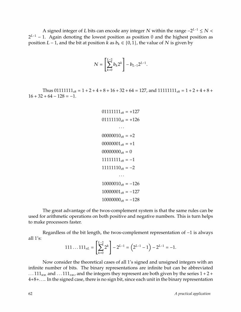
A signed integer of L bits can encode any integer N within the range −2L−1 ≤ N <

2L−1 − 1. Again denoting the lowest position as position 0 and the highest position asposition L − 1, and the bit at position k as bk ∈ {0, 1}, the value of N is given by

N =

[L−2∑k=0

bk2k]− bL−12L−1.

Thus 01111111s8 = 1 + 2 + 4 + 8 + 16 + 32 + 64 = 127, and 11111111s8 = 1 + 2 + 4 + 8 +16 + 32 + 64 − 128 = −1.

01111111s8 = +127

01111110s8 = +126

· · ·00000010s8 = +2

00000001s8 = +1

00000000s8 = 0

11111111s8 = −1

11111110s8 = −2

· · ·10000010s8 = −126

10000001s8 = −127

10000000s8 = −128

The great advantage of the twos-complement system is that the same rules can beused for arithmetic operations on both positive and negative numbers. This is turn helpsto make processors faster.

Regardless of the bit length, the twos-complement representation of −1 is alwaysall 1’s:

111 . . . 111sL =

[L−2∑k=0

2k]− 2L−1 =

(2L−1 − 1

)− 2L−1 = −1.

Now consider the theoretical cases of all 1’s signed and unsigned integers with aninfinite number of bits. The binary representations are infinite but can be abbreviated. . . 111u∞ and . . . 111s∞, and the integers they represent are both given by the series 1+ 2+4+8+. . .. In the signed case, there is no sign bit, since each unit in the binary representation

62 A practical application

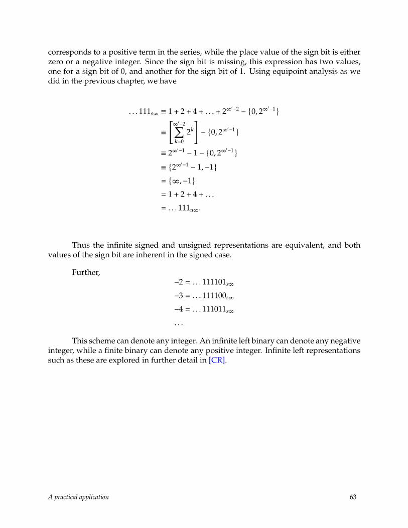
corresponds to a positive term in the series, while the place value of the sign bit is eitherzero or a negative integer. Since the sign bit is missing, this expression has two values,one for a sign bit of 0, and another for the sign bit of 1. Using equipoint analysis as wedid in the previous chapter, we have

. . . 111s∞ ≡ 1 + 2 + 4 + . . . + 2∞′−2 − {0, 2∞′−1}

≡[∞′−2∑k=0

2k]− {0, 2∞′−1}

≡ 2∞′−1 − 1 − {0, 2∞′−1}

≡ {2∞′−1 − 1,−1}= {∞,−1}= 1 + 2 + 4 + . . .

= . . . 111u∞.

Thus the infinite signed and unsigned representations are equivalent, and bothvalues of the sign bit are inherent in the signed case.

Further,−2 = . . . 111101s∞

−3 = . . . 111100s∞

−4 = . . . 111011s∞

. . .

This scheme can denote any integer. An infinite left binary can denote any negativeinteger, while a finite binary can denote any positive integer. Infinite left representationssuch as these are explored in further detail in [CR].

A practical application 63

COMPARISON TOCONVENTIONAL THEORY

Three approaches

We will consider the following three approaches to divergent series.

1. Limits. In this approach, any infinite series is considered to be the limit of itspartial sums:

∞∑k=1

ak := limn→∞

n∑k=1

ak .

If the limit exists, the series is said to be convergent, and otherwise divergent.A divergent series has no limit and therefore, strictly speaking, no sum. Moreinformally we may say that the sum is∞, but this symbol is usually not defined asa number.

2. Methods. In this approach, a convergent series is still considered to be a limit, buta divergent series may be said to have a finite sum in a restricted sense. It has thissum if some calculational procedure based on the terms of the series yields a finitesum. The procedure is called a method of summation. Ideally, a method appliedto a convergent series should yield the same sum as the limit, in which case themethod is said to be regular. When it is applied to at least some divergent series,it may yield a finite sum. Since the sum of a divergent series may vary from onemethod to another, the equality of the series with its sum is said to exist only in thesense of the method.

3. Numeristic. In this approach, any infinite series is considered simply as a purelyinfinite arithmetic sum, without regard to a limit. It regards infinite sums as actual.It uses two primary techniques: (1) recursion and (2) an analytic approach calledequipoint summation.

The limits approach was developed in the early nineteenth century and becamenearly universal as direct calculation with the infinite and the infinitesimal was replacedwith limits and set theoretical notions. Today, many professional mathematicians areunaware of any alternatives.

The methods approach developed in parallel to the limit approach but remainedmuch less popular. It is today known as the theory of divergent series. By far the mostcomprehensive treatment of this approach is [Mo], now considered a standard reference.

64 Comparison to conventional theory

The numeristic approach is the one we develop in this monograph. As see inThe Euler extension method of summation, the recursion technique of the numeristicapproach is not really new, but a better understanding and enhancementof an old tech-nique.

Hardy [H, p. 6–7] defines the notation∑am = s (P) to mean that the series

∑am

has a sum s in the sense of a method P . This symbolism means that equality holds onlyin a certain sense, because changing the sense, the method of determining the sum, canchange the value s that we define as the sum. This weakens the meaning of equality, sinceit is relative to a method of computation, and not, as is normally the case, independent ofit.

The methods approach has several weaknesses:

1. An unworkable conception of weak equality.

2. The failure of all methods, except the Euler extension method, to account for Equa-tion 2.

3. A faulty understanding of the Euler extension method, including a circular defini-tion in [H], and failure to realize this method as an extension of arithmetic.

We further examine these points in later chapters and show how the numeristicapproach avoids all of them.

Other approaches

A few other approaches to divergent series deserve consideration.

Transformation to convergent series. In this approach, a divergent series is consid-ered as an encoded form of a convergent series, using the transformation

11 − a =

(− 1a

)1

1 − 1a

.

This approach has the disadvantage of conceptualizing simple arithmetic state-ments as something different from what they state, and therefore of introducing extrasteps of calculation. Another disadvantage is that an expression which combines conver-gent and divergent series, such as

∑+∞−∞ a

n, must be considered as the sum of two separateseries.

Congruence. In this approach, we observe that the partial sums∑j

0 2n are eachcongruent to −1 mod 2j+1. The drawback of this approach is that it requires us to define

Comparison to conventional theory 65

an equality through a congruence. It is also not immediately clear how to extend it to any

other case than∑j

0 2n, since for integral bases greater than two, the sum is a fraction.

Adjusted series. Another approach is to return to the twos-complement arithmeticdescribed above, and generalize its sign bit mechanism. This seems at first to be a combi-nation of the limit and numeristic approach, but it actually ends up being essentially justthe numeristic approach.

If we define

f(k) =

ak , k < nak

1 − a, k = n

thenn∑k=0

f(k) =

(n−1∑k=0

ak)

+an

1 − a =1 − an1 − a +

an

1 − a =1

1 − a.

This value does not depend on n—for all values of n, the sum is constant. In theinfinite case, the last term does not exist. Hence we say that

∞∑k=0

f(k) =∞∑k=0

ak =1

1 − a.

This satisfies the limits approach, because the infinite case is the limit of the finitecase. But a limits approach alone does not suggest how to modify the definition of

∑∞k=0 a

k

so that the result is constant. The numeristic approach supplies the crucial last term andthus satisfies this requirement.

Objections

Approaches to the theory of divergent series historically have faced various objec-tions which did not seem to allow simple algebraic treatment. Here we examine some ofthese objections and their numeristic resolutions.


Incorrect sum of absolute arithmetic series

It is sometimes claimed that the absolute arithmetic series 1+2+3+ . . . has the sum112 . Equipoint summation does not support this claim, finding instead that this series hasonly an infinite value. See Absolute arithmetic series. Nevertheless, 1

12 is associated withthis series, as is shown in Ramanujan summation.

Apparent incompatibility of linearity and stability

In the method approach to divergent series, we say that a summation method islinear if

∞∑n=0

an +∞∑n=0

bn =∞∑n=0

(an + bn)

for any two series an and bn, and we say that the method is stable if

a0 +∞∑n=1

an =∞∑n=0

an,

i.e. adding a term to the beginning of the series increases the sum of the series by the sameamount.

The method approach claims that a summation method that is both linear andstable cannot sum the series 1 + 2 + 3 + . . .. The argument is that if

1 + 2 + 3 + . . . = x,

then by stability0 + 1 + 2 + . . . = 0 + x = x.

By linearity, one may subtract the second equation from the first to give

1 + 1 + 1 + . . . = x − x = 0.

Again by stability,0 + 1 + 1 + 1 + . . . = 0,


and subtracting the last two series gives

1 + 0 + 0 + . . . = 0,

contradicting stability.

Numeristically, the problem with this argument is that the first and second seriesboth have only one value,∞, as shown in Absolute arithmetic series. Subtracting the sec-ond from the first yields 6∞ rather than zero. The third series, as shown in Absolute sumof units, also has only the value∞, which is an element of 6∞ and is thus consistent withthe previous subtraction. Likewise the fourth series has only the value∞, so subtractingit from the third again yields 6∞, which includes 0 and 1.

Apparent multiple values

Hardy [H, p. 16] points out several examples of divergent series which appear togive multiple values. For example, it appears that

x + (2x2 − x) + (3x3 − 2x2) + (4x4 − 3x3) + . . . = 0

andx + (3x2 − x) + (7x4 − 3x2) + (15x8 − 7x4) + . . . = 0

for 0 ≤ x < 1, but for x = 1 these give 1 + 1 + 1 + . . . = 0 and 1 + 2 + 4 + . . . = 0. But he doesnot recognize that

x + (2x2 − x) + (3x3 − 2x2) + (4x4 − 3x3) + . . .

= (x − x) + (2x2 − 2x2) + (3x3 − 3x3) + (4x4 − 4x4) + . . .

= 0 + 0 + 0 + . . . = 0 ×∞,

and similarly

x + (3x2 − x) + (7x4 − 3x2) + (15x8 − 7x4) + . . .

= (x − x) + (3x2 − 3x2) + (7x4 − 7x4) + (15x8 − 15x8) + . . .

= 0 + 0 + 0 + . . . = 0 ×∞,


which of course are indeterminate, not merely zero.

Apparently incorrect sum of the Grandi series

Using Equation 2, we have shown that we can calculate that 1−1+1−1+ . . . = 12 . It

is frequently objected that this cannot be the only correct result, since we could also have1 − 1 + 1 − 1 + . . . = (1 − 1) + (1 − 1) + . . . = 0 + 0 + . . . = 0. This objection comes from oneor both of two points of view: (1) an infinite sum is a limit; or (2) the sum of an infinitenumber of zeros is zero. The first point of view overlooks the important fact that the typeof sum we are considering here is not a limit. The second point of view overlooks the factthat an infinite sum of zeros is∞× 0, which is indeterminate. See also Alternating sum ofunits, where we explore the Grandi series with equipoint summation.

Callet’s objection

Euler was the first to systematically use Equation 2 for divergent series and wasthe first to state this case of it. Some time afterwards, Callet challenged this view, citingthe series

1 − a2 + a3 − a5 + a6 − a7 + a8 − . . . .Setting x to this series, we have

x = 1 − a2 + a3 − a5 + a6 − a8 + a9 − . . .= 1 − a2 + a3(1 − a2 + a3 − a5 + a6 − . . .)= 1 − a2 + a3x.

Then x − a3x = 1 − a2, and

x =1 − a2

1 − a3=

1 + a1 + a + a2

.

When a = 1, we would then have

1 − 1 + 1 − 1 + . . . =23.

Lagrange replied that actually

1 − a2

1 − a3= 1 + 0a − a2 + a3 + 0a4 − a5 + a6 + 0a7 − a8 + a9 + . . . ,


which for a = 1 becomes

1 + 0 − 1 + 1 + 0 − 1 + 1 + 0 − 1 + 1 + . . . =23.

This differs from 1 − 1 + 1 − 1 + . . . by the addition of an infinite number of zeroes,which, as we have seen above, is not zero but indeterminate. Besides this, for a = 1,

1+a1+a+a2 = 2

3 , but 1−a2

1−a3 is indeterminate.

Indeterminacy of 0 ×∞

A common thread in these considerations is the indeterminacy of 0 · ∞. FromEquation 3 we have

∞∑k=0

0ak = 0 + 0a + 0a2 + 0a3 + . . . = 0(1 + a + a2 + a3 + . . .

)=

01 − a,

which is zero except for a = 1, where it is indeterminate. Thus the sum of an infinitenumber of zeros may be zero or indeterminate. It is indeterminate when the ratio betweenthe zeros is constant, and this is the case in the above examples. An example where this isnot the case is a terminating decimal, which is also a repeating decimal with repetend 0:

0.5 = 0.5000 . . . =12+

0100

(1 +

110

+1

100+

11000

+ . . .)

=12+

01 − 1

10

=12.

For further information on infinite sums of zeros, see Sum of zeros above. Forfurther information on terminating decimals, see [CR].

Apparent inconsistency with Riemann zeta function

Hardy [H, p. 16] states that 1 + 1 + 1 + . . . = − 12 , because the well-known Riemann

zeta function, which he states as

ζ(x) =∞∑k=1

kx,


has the value ζ(0) = − 12 . The problem with this value is that it is calculated from the

definition

ζ(x) =1

Γ(x)

∫∞0

ux−1

eu − 1du,

which is equivalent to the first expression for x > 1, but not elsewhere.

Paradox of comparison of series and integrals

In equipoint analysis ([CE]), a definite integral is an infinite series in which eachterm is zero, while in a convergent or divergent series, an infinite number of terms arenonzero. When the terms can be directly compared, this may lead to a paradoxical con-dition wherein both a series and an integral yield a finite result. For example, considerthat

∞∑n=1

2−n = 1 <∫1

02 dx =

∞′∑n=1

2∞′ = 2,

even though, if we look at individual terms,

2−n ≥ 2∞

for all n, with equality holding only for infinite n.

We have already seen that the first series actually has two values, one infinite andone finite. See Infinite series have infinite values.

The conventional theory of divergent series

For several centuries there has been a theory of divergent series, which attemptsto show how and why we can find a sum for many types of divergent series. It is oftensaid that the theory of divergent series started with Euler, whose findings on the subjectare probably best represented in [Eu55] and [Eu60]. This theory has attracted other wellknown names, including Poisson, Abel, and Hardy. Hardy’s posthumous book [H] of1949 is generally considered a standard work.

Euler and other mathmaticians of the 18th century generally either took a basicallynumeristic approach to divergent series, or rejected such series, or vacillated. In the 19thcentury, the limits approach developed and gradually came to dominate the approach toinfinite arithmetic. In the 20th century, the methods approach developed and attractedsome attention, but still remained poorly known and did not come to dominate over thelimits approach.


In recent years, the methods approach seems to be attracting much more attention.One example of this transition occurred between two editions of the Encyclopedic Dictio-nary of Mathematics, a standard general mathematics reference work. In the first edition[ED77], published in 1977, the article Summability describes the methods approach to di-vergent series, while the article Infinite series gives only the conventional limits approachwithout even a reference the summability article, and the index does not reference thesummability article under series, only under summability. In the second edition [ED87] of1987, the summability material has been merged into the Infinite series article. Both [ED77]and [ED87], in their succinct but formalistic way, define a method as a linear transfor-mation and therefore omit the Euler extension method, described below. They also useweak equality, the assertion that equality established through a method is relative to themethod.

Hardy does not define method but does use weak equality. Hardy additionallyadmits the Euler extension method. This method is best suited to power series, which isthe key to the whole theory.

Methods of summation

Hardy [H] defines several dozen methods of summation. We will now examine asignificant cross section of these methods, and a few that have been developed since [H]was published. This includes all the methods commonly encountered in the literatureand many other more obscure methods. We will apply each one to the series

∞∑k=0

ak , |a| > 1. (89)

Surprisingly, we will find that only one of these methods is capable of summingthis series. That method is the Euler extension method, discussed below.

A key criterion for assessing the validity of any method is regularity. A method Pis regular if, for any convergent series

∑am,∑

(P)am = lim∑am, i.e. if the method sums

any convergent series to its ordinary value as a limit. Most, but not all, methods definedin [H] are regular.

For each of these methods:

• We give a page reference to [H], except for two methods which are not in [H].

• We indicate whether the method is regular.


• We give a definition of the method when it is fairly simple. Otherwise, we expressour conclusions in the same notation that [H] uses.

• We apply each method to Equation 89.

• We denote partial sums as sn :=∑n ak .

Euler method (E), which we call the Euler extension method: [H, p. 7]. For a fulldiscussion, see The Euler extension method of summation. Regular. Sums (89) to am

1−a .

Cesaro mean (C, 1): [H, p. 7]. Defined as∑

(C,1)an = lim

n→∞

s0 + s1 + s2 + . . . + snn + 1

.

Regular. Diverges for (89).

Abel sum (A): [H, p. 7]. Defined as∑

(A)an = limx→1−∑anx

n if∑anx

n is conver-gent for 0 ≤ x < 1. Regular. Does not apply to (89) since

∑anx

n =∑anxn =

∑(ax)n is

not convergent for all x ∈ [0, 1).

Euler’s polynomial method (E, 1): [H, p. 7]. Regular. Diverges for (89), since bn =(a + 1)n > 2n.

Hutton’s method (Hu, k): [H, p. 21]. Regular. A limit of positive terms for (89),and thus diverges.

Ramanujan’s method (R, a): [H, p. 327]. Hardy misrepresents Ramanujan’s orig-inal method. This is examined in detail in the next chapter, Ramanujan summation.

Borel integral method (B′): [H, p. 83]. Regular. Sums (89) to 11−a only when Rea <

1.

Borel exponential method (B): [H, p. 80]. Regular. Sums (89) to 11−a only when

Rea < 1.

Norlund means (N, pn): [H, p. 64]. Scheme requiring choice of {pn}. Regular forsome {pn}. The partial quotients for (89) tm are always positive, and thus cannot yield

11−a , which is negative.

Abel means (A, λn): [H, p. 71]. Scheme requiring choice of {λn}. Regular. For (89),yields only positive terms, so the method yields a positive limit or no limit.

Lindelof method (L): [H, p. 99]. Regular. Same as (A,n lnn) for (89), which fails inall cases.

Mittag-Leffler method (M): [H, p. 79]. Regularity not stated in [H]. Similar toLindelof method. Hardy shows that L and M methods take (89) to 1

1−a , but only on a


region ∆ in the complex plane, called the Mittag-Leffler star of an for a ∈ C. This regiondoes not include any point in (1,∞).

Riemann method (R, k): [H, p. 89]. Regular for k > 1. For (89), an eventually

overwhelms(

sinnhnh

)k, so the limit diverges.

Euler’s general polynomial method (E, q): [H, p. 178]. Regular. Requires q > 0 andsums (89) to 1

1−a only within a circle with center at −q and radius q + 1, which excludesa > 1.

General Cesaro means (C, k): [H, p. 96]. Regular for k > 0. Limit of the quotient oftwo positive terms for (89); diverges.

Holder means (H, k): [H, p. 94]. Regularity not stated in [H]. Limit of positiveterms for (89); diverges.

Ingham’s method (I): [H, p. 399]. Not regular. Limit of the sum of positive termsfor (89); diverges.

Second Norlund method (N, pn): [H, p. 57]. Regular. Yields a positive fraction for(89) and any set of positive {pn}, and thus cannot yield 1

1−a , which is negative.

De la Vallee-Poussin’s method (VP): [H, p. 88]. Regular. Limit of the sum ofpositive terms for (89), which is never negative.

Bernoulli summability (Be): Not in [H]. Defined by

∑(Be)

an = limN→∞

N∑n=0

sn

(N

n

)pn(1 − p)N−n,

where sn =∑n ak and 0 < p < 1. Always yields a positive result for (89) and thus cannot

assume a negative value.

Dirichlet summability (D): Not in [H]. Defined by∑

(D)an = lim

x→1+

∞∑n=1

snns

, where

sn =∑n ak . Always yields a positive result for (89) and thus cannot assume a negative

value.


Ramanujan summation

Hardy defines a Ramanujan method of summation, but Hardy’s definition differssignificantly from Ramanujan’s original definition. Hardy also states that Ramanujan’sdefinition is a method of summing a series, whereas Ramanujan’s claim is more modest.Since Hardy somewhat misrespresents Ramanujan’s work, we now examine the discrep-ancies in detail.

Ramanujan’s original method is described in ([Be, p. 133-136]). This posthumousedition of Ramanujan’s notebooks by B. Berndt includes much commentary by Berndt.

This section functions as a correction of Hardy. He ([H, p. 327]) defines a Ramanu-jan sum (R, a) of a series, which depends on a, and says there is a natural value of afor every series but does not describe a general procedure for finding this a. Hardy’sdefinition is reproduced below.

Hardy says that Ramanujan’s work with divergent series was based on this defini-tion, but (1) Ramanujan uses a simpler definition, also given below, that does not dependon a parameter, and (2) Ramanujan calls the number he computes the “constant” of a se-ries and denotes it as an operator on a function. He relates it to but does not equate itwith a sum of a divergent series.

Both of these definitions are based on the Euler-Maclaurin formula, which relatesa sum with finite limits and an integral over a finite interval. This formula uses theBernoulli numbers Bn and periodic Bernoulli polynomials Pn. Hardy uses a definitionof Bernoulli number that is now generally considered obsolete and is now written B∗k .

These two are related by B∗k = (−1)k+1B2k . Here we express Hardy’s definitions in thenewer notation.

The Euler-Maclaurin formula is usually given as:

x∑k=0

f(k) =∫x

0f(t)dt +

12[f(x) + f(0)

]+

p∑k=1

B2k

(2k)!

[f (2k+1)(x) − f (2k+1)(0)

]+∫x

0

P2p+1(t)(2p + 1)!

f (2p+1)(t)dt.


Subtracting f(0) gives the form that Ramanujan/Berndt uses:

x∑k=1

f(k) =∫x

0f(t)dt +

12[f(x) − f(0)

]+

p∑k=1

B2k

(2k)!

[f (2k+1)(x) − f (2k+1)(0)

]+∫x

0

P2p+1(t)(2p + 1)!

f (2p+1)(t)dt.

In both cases, p is arbitrary. The last term is a remainder which is often denotedRpf(x), while the second last term is denoted Spf(x) − Spf(0).

When x = ∞, both the sum and the integral have infinite limits. The sum is con-vergent if and only if the integral is also convergent.

Ramanujan/Berndt sets p = ∞ and examines two cases, f(x) = 1 and f(x) = x.We examine two additional cases, f(x) = ex and its general case f(x) = bx for a perfinitenonunit constant b.

First we compute R∞ indirectly by evaluating

x∑k=1

f(k) −∫x

0f(t)dt − 1

2[f(x) − f(0)

]− S∞f(x) + S∞f(0).

We then have:

For f(x) = 1:

R∞ = x − x − 0 − 0 + 0 = 0

For f(x) = x:

R∞ =x2 + x

2− x

2

2+x

2− 1 + 1 = 0


For f(x) = ex:

R∞ =ex+1 − exe − 1

− ex − 1 − 12(ex − 1) −

∞∑k=1

B2k

(2k)!(ex − 1)

= (ex − 1)e

e − 1− (ex − 1) − (ex − 1)

12− (ex − 1)

∞∑k=2

Bkk!

= (ex − 1)[

e

e − 1− 1 − 1

2−(

1e − 1

− 1 +12

)]= (ex − 1)

e − e + 1 − 1e − 1

= 0

For f(x) = bx:

R∞ =bx+1 − bxb − 1

− bx − 1ln b

− 12(bx − 1) −

∞∑k=1

B2k

(2k)!(ln b)2k−1(bx − 1)

= (bx − 1)b

b − 1− (bx − 1)

1ln b

− (bx − 1)12− (bx − 1)

1ln b

∞∑k=2

Bkk!

(ln b)k

= (bx − 1)[

b

b − 1− 1

ln b− 1

2− 1

ln b

(1

b − 1− 1 +

ln b2

)]= (bx − 1)

2b ln b − 2(b − 1) − (b − 1) ln b − 2 + 2(b − 1) − (b − 1) ln b2(b − 1) ln b

= (bx − 1)ln b − 1

(b − 1) ln b

From the Euler-Maclaurin formula, Ramanujan/Berndt extracts the portion of theright side which is independent of x and calls it the constant C of the series:

C = −12f(0) −

∞∑k=1

B2k

(2k)!f (2k+1)(0).


We then have:

For f(x) = 1 : C = −12− 0 = −1

2

For f(x) = x : C = −0 − 112

= − 112

For f(x) = ex : C = −12−(

1e − 1

− 1 +12

)=−1e − 1

For f(x) = bx : C = −12− 1

ln b

(1

b − 1− 1 +

ln b2

)=

b − 2(b − 1) ln b

− 1

Hardy refines Ramanujan’s C by adding a parameter a. Berndt notes this (p. 135)and gives Hardy’s Ca as

Ca =∫a

0f(t)dt − 1

2f(0)

−p∑k=1

B2k

(2k)!f (2k−1)(0) +

∫∞0P2p+1(t)f (2p+1)(t)dt.

Ca is independent of p, since p is arbitrary in the Euler-Maclaurin formula.

Hardy’s actual definition is somewhat different (p. 326). To distinguish it fromBerndt’s, we call it C′:

C′a =∫a

1f(t)dt +

12f(1)

−p∑k=1

(−1)k−1Bkk!

f (2k−1)(1) − 1(2n + 2)!

∫∞0ψ2p+2(t)f (2p+2)(t)dt,

where ψn(x) = ψn(x − bxc) and t ext−1et−1 =

∑∞n=0 φn(x)

tn

n! .


Hardy compares∑

1 to∫

1, whereas Berndt compares∑

1 to∫

0. This means we musttranspose f so that Hardy’s f(x) is Berndt’s f(x − 1). It also means that Hardy uses thefirst form of the Euler-Maclaurin forumula, whereas Berndt uses the second form. Aftertransposing f , we must add f(0) to Berndt’s formula to get Hardy’s formula. We ignorediscrepancies in the remainder, since we calculate it indirectly as above.

We can therefore express Ca and C′a as:

Ca =∫a

0f(t)dt − 1

2f(0) −

p∑k=1

B2k

(2k)!f (2k−1)(0) + R∞

C′a =∫a

0f(t)dt +

12f(0) −

p∑k=1

B2k

(2k)!f (2k−1)(0) + R∞

= Ca + f(0)

and we compute:

For f(x) = 1 : C0 = −12− 0 = −1

2

C′0 =12

For f(x) = x : C0 = − 112− 0 = − 1

12

C′0 = − 112

For f(x) = ex : C0 =−1e − 1

+ 0 =−1e − 1

C′0 =−1e − 1

+ 1 =e − 2e − 1

For f(x) = bx : C0 =b − 2

(b − 1) ln b− 1 − ln b − 1

(b − 1) ln b=−b ln b + b − 1(b − 1) ln b

C′0 =−b ln b + b − 1(b − 1) ln b

+ 1 =− ln b + b − 1(b − 1) ln b

+ 1

Claiming that this is a sum is not true to Ramanujan’s work because:

1. Ramanujan never claimed that his constant was a sum.


2. The constant formula only represents a portion of the difference between a sumand an integral, not the sum itself.

3. The portion it represents does not depend on the upper bound of the sum, whichmay be finite or infinite, whereas a sum of course generally depends on its upperlimit.

The Euler extension method of summation

We now examine in detail the Euler extension method of summation, which Hardydenotes as E. We have seen how every other method commonly used in the current theoryof divergent series fails to derive

∑an = 1

1−a for |a| ≥ 1. Strangely, even though this is theonly such method that can derive this sum, it is usually omitted from works on divergentseries. For instance, [ED87, p. 1415] defines a method as a linear transformation and thusdefines away this method.

We will see that this method is poorly understood. We will develop a better under-standing of it and see how this yields a satisfactory theory of divergent series. We startwith Hardy’s definition [H, p. 7]:

If∑anx

n is convergent for small x, and defines a function f(x) of the complexvariable x, one-valued and regular in an open and connected region containing the originand the point x = 1; and f(1) = s; then we call s the E sum of

∑an. The value of s may

naturally depend on the region chosen.

Unfortunately, this definition is circular. If the series defines f , then f(x) =∑anx

n

within some region, and if this region contains x = 1, then f(1) =∑an by definition. This

does not extend the definition of the series from the convergent case to the divergent case,but instead assumes that we already have a definition of the divergent case.

Euler’s own definition of his method is quite different. He identifies an infiniteseries, convergent or divergent, with a finite expression from which it is “expanded,” andthe sum of the series with the value of the expression. He defends such an assignment ofa sum to a divergent series as consistent and useful:

Let us say, therefore, that the sum of any infinite series is the finite expression, bythe expansion of which the series is generated. In this sense, the sum of the infinite series1 + x + x2 − x3 + . . . will be 1

1−x , because the series arises from the expansion of the fraction,whatever number is put in place of x. If this is agreed, the new definition of the word sumcoincides with the ordinary meaning when a series converges; and since divergent serieshave no sum, in the proper sense of the word, no inconvenience can arise from this newterminology. Finally, by means of this definition, we can preserve the utility of divergent


series and defend their use from all objections.

[Eu55, Ch. 3, Sect. 111, p. 78–79] tr. [BL, p. 142]

The above passage appears in a book on analysis which Euler wrote in 1755. Fiveyear later, Euler wrote a paper on divergent series, in which he appears to be assumingthe role of mediator between two opposing factions, one which opposes assigning anysum to a divergent series, and one which supports it. After carefully considering thearguments of both sides, he comes down firmly on the side of supporting the assignmentand gives several reasons for his decision. The following three quotes from this paper arehighlights of his reasoning. The first quote makes it clear that his method of expanding

11−x into 1 + x + x2 − x3 + . . . is polynomial division:

Of the second type [in his list of types of infinite series, the second type beingoscillating series] is this series, 1 − 1 + 1 − 1 + − . . ., first considered by Leibniz, whose sum

he gave as equal to 12 , with the support of the following fairly sound reasoning: first, this

series appears if the fraction 11+a is expanded in the usual way by continued division into

the following series 1 − a + a2 − a3 + a4 − a5 + . . ., and the value of the letter a is taken equalto unity.

[Eu60, §3, p. 207] tr. [BL, p. 145]

In the next passage, Euler addresses the objection that using the above procedureon a series such as 1+2+4+8+ . . ., consisting entirely of positive terms, leads to a negarivesum, −1. He points out that this is not as unreasonable as it may appear, since a transitionfrom positive to negative can occur through the infinite as well as through zero:

However, it seems in accord with the truth if we say that the same quantities whichare less than zero can be considered to be greater than infinity. For not only from alge-bra but also from geometry, we learn that there are two jumps from positive quantities tonegative ones, one through nought or zero, the other through infinity, and that quantitieswhether increasing from zero or decreasing come back on themselves and return to thesame destination 0 . . .

[Eu60, §8, p. 210] tr. [BL, p. 147]

This is in accord with the projectively extended real number system that we haveused here and defined in [CN]. In this system, ∞ is both positive and negative, and,depending on the mapping method, maps to either one or two points on a unit circle thatis tangent to the real number line.

In the following quote from his paper, Euler repeats his contention that his methodof assigning a sum to a divergent series is meaningful and useful:


But I think all this wrangling can be easily ended if we should carefully attend towhat follows. Whenever in analysis we arrive at a rational or transcendental expression,we customarily convert it into a suitable series on which the subsequent calculation canmore easily be performed. Therefore infinite series find a place in analysis inasmuch asthey arise from the expansion of some closed expression, and accordingly in a calculationit is valid to substitute in place of the infinite series that formula from which the seriescame. Just as with great profit rules are usually given for converting expressions closedbut awkward in form into infinite series, so likewise the rules, by whose help the closedexpression, from which a proposed infinite series arises, can be investigated, are to bethought highly useful. Since this expression can always be substituted without error forthe infinite series, both must have the same value: it follows that there is no infinite seriesfor which the closed expression equivalent to it cannot be conceived.

[Eu60, §11, p. 211–212] tr. [BL, p. 148]

Euler emphasizes the equivalence of a divergent series with its finite form. If thefinite form is not known, his method may not appear to be useful. However, when he in-

dicates that 1+a+a2 +a3 + . . . is obtained from1

1 − a by polynomial division, he seems to

imply that the arithmetic of divergent series is consistent with the rest of algebra. There-fore, any algebraic technique which transforms a series to a finite expression should bevalid.

The recursion approach we have used here to obtain finite values for infinite se-ries is thus essentially equivalent to the extension method Euler proposes. The recursionapproach enhances Euler’s method by showing that, whenever an infinite series is alge-braically equivalent to an expression that has a finite value, that expression also has aninfinite value. We have seen that this approach, when properly applied, does not yieldany known inconsistencies. This method is clearly regular, since it does not involve anytransformation of a divergent series to a convergent one.

Euler’s extension method is essentially the extension of meaning in a consistentway to forumulas which were previously considered meaningless. This extension is sim-ilar in principle to the extension of the number system to irrational, negative, and imagi-nary numbers, all of which initially met with opposition.

• In the 5th century BC, the Greek mathematician Hippasus’s proof of theexistence of irrational numbers led to his being persecuted by fellowPythagoreans. It took another century for Greek mathematicians to acceptirrational numbers.

• Negative numbers were rejected as meaningless by ancient Greek mathe-maticians. They were used in ancient and medieval times in India, China,and Islamic countries, but they were not accepted in Europe until the 16thand 17th centuries.

• Imaginary numbers became known in Europe in the 16th century, but theywere usually regarded as meaningless until the 18th century.


Euler’s extension method involves no limits and no transformation of terms orpartial sums. It can calculate the sum of series that no other method can, and there is noknown series that any other method can sum that this method cannot. The numeristicapproach starts with Euler’s extension method and adds an infinite value to whateverfinite value Euler’s method may find, and yields an infinite value alone for those forwhich that Euler’s methods finds no value.

There is no need for a weakened form of equality, since we assume that a divergentseries is strictly equal to its algebraic sum. The results of this approach can be appliedwithout ambiguity, since the equalities it establishes are as stong as all other equalities.

In this approach, if we wish to use other methods of summation, we denote themas modified summation rather than weakened equality. Szasz [Sz, p. 2] uses the notationP(∑am) = s. This leaves equality strong, but it also implies that we first compute the

value of∑am and then apply P after we compute the sum, whereas the real situation

is that a method P operates first on the terms of the series, and then either sums themodified terms or performs some other operation on them. This means that P is really amodified form of summation. The notation

∑(P)am = s properly conveys that a method

P sums a series with terms am to the value s.


Analytic continuation

−1 0 1 2 3

−i

i

2i

........................................................................................................................................................

...............

............

...........

.....................................................................................................................

................

.............................................................................................................................................................................

...................

.............

............

..........

................................................................................................................

.................

.............................................................................................................................................................................................................................................................................

....

....

.............................................................

..................

...............................................................................................................................................................................................................................................................................................

..................

.............

............

..........

.........................................

A

B

C

FIG. 11:Analytic extension of f(z) = 1

1−zinto neighborhoods of z = 0, 1 + i, 2

The Euler extension method bears some resemblance to analytic continuation, buthas an important difference from it. In complex analysis, given an analytic function, an-alytic continuation is a procedure of deriving multiple convergent series in overlappingneighborhoods, in each of which the series converges to the same analytic function.

Figure 11 shows this process for f(z) =1

1 − z . We start with the interior of circle

A, the neighborhood |z| < 1, where the series

∞∑k=0

zk = 1 + z + z2 + z3 + . . . (A)

converges to f(z). Then we move to the interior of circle B, the neighborhood |z−1−i| < 1,


which overlaps the interior of A. Here the convergent power series for f(z) is

∞∑k=0

(z − 1 − i)k = 1 + (z − 1 − i) + (z − 1 − i)2 + (z − 1 − i)3 + . . . . (B)

By a well known theorem of complex analysis, if f(z) is analytic in the interior of A, andthe interiors of A and B overlap, then both series (A) and series (B) converge to the samefunction, f(z), within the overlapping area.

In this way, one convergent series after another for f(z) can then be developed. InFigure 11, the interior of circle C is |z − 2| < 1, where the series

∞∑k=0

(z − 2)k = 1 + (z − 2) + (z − 2)2 + (z − 2)3 + . . . (C)

converges to f(z). Again, series (B) and series (C) both converge to the same function,f(z), in the overlap of the interiors of B and C. However, the interiors of A and C do notoverlap, which means that series (A) diverges everywhere that series (B) converges andconversely.

We have thus analytically extended f(z), but to do so, we must proceed in steps,and we derive a different power series at every step.

This contrasts with the Euler extension method, which deals with divergent series,as well as convergent series, and does not proceed in steps. Instead, the Euler extensionmethod, as we have developed it here, recognizes that infinite series, and the numeristicarithmetic and algebra used to handle them, are valid whether the series are convergentor divergent. In this approach, series (A), (B), and (C) are valid for f(z) throughout thecomplex plane, whether they are convergent or not.


SUMMARY OF THE NUMERISTICAPPROACH TO DIVERGENT SERIES

The numeristic approach to divergent series developed in this monograph can besummarized as follows.

1. Use only strict equality, not any form of weakened equality.

2. Use the projectively extended real numbers and numeristic classes to extend arith-metic to any operation, including the exponential of infinity, which has two values.

3. Use algebraic transformations to compute the equality of a series with its sum,instead of defining the sum as a limit.

4. Denote methods of summation other than the Euler extension method as modifiedforms of summation, instead of modified forms of equality.

5. Use equipoint arithmetic to determine the sum of an infinite number of zeros, in-stead of assuming that the sum is always zero.

86 Summary of the numeristic approach to divergent series

NUMERISTICS IN GENERAL

A deeper aspect of the numeristic approach is the view that numbers and arith-metic stand on their own and do not require definitions to exist. Although our discus-sions require that we define our terms, definitions are not a substitute for mathematicaltruth. The truth of mathematical expressions must ultimately be verified by observationof nature, just as in any other science. In other words, mathematical truth cannot simplybe defined into existence.

In this light, we examine Hardy’s remarks in [Mo, p. 5–6] concerning the role ofdefinitions in the methods approach to divergent series, which, in the numeristic view,contain a mixture of both valid and excessive claims about definitions.

[I]t does not occur to a modern mathematician that a collection of mathematicalsymbols should have a ‘meaning’ until one has been assigned by definition. It was not atriviality even to the greatest mathematicians of the eighteenth century. They had not thehabit of definition; it was not natural to them to say, in so many words, ‘by X we meanY’. There are reservations to be made, . . . but it is broadly true to say that mathematiciansbefore Cauchy asked not ‘How shall we define 1 − 1 + 1 − . . .?’ but ‘What is 1 − 1 + 1 − . . .?’,and that this habit of mind led them into unnessary perplexities and controversies whichwere often really verbal. [Emphasis his.]

While Hardy further acknowledges that the value of 12 seems “natural,” he says

that assigning this as the sole value of the series actually has problems, which he attributesto lack of proper definition. His solution is to use methods of summation, with its conceptof weak equality. However, his definition of the Euler extension method is quite differentfrom Euler’s, and it is circular. He seems to miss its essence as a simple extension ofarithmetic.

The numeristic approach gains support from the recent development of MaharishiVedic Mathematics, a formulation of ancient Vedic philosophies and technologies of con-sciousness in mathematical terms [CI, My] by Maharishi Mahesh Yogi, the founder of theTranscendental Meditation program. In this approach, pure consciousness is the basicexperience and governing intelligence of life. The technologies of Maharishi Vedic Math-ematics, including Transcendental Meditation, give the experience of pure consciousness.Pure consciousness is equated with zero, which is characterized as the point of infinity andthe Absolute Number, the support of all number systems, and thereby all of natural law.Number thereby becomes a natural experience of self-referral available to everyone.

In the author’s experience, Maharishi Vedic Mathematics gives both experienceand understanding that makes one at home with the infinite. The infinite sums of thenumeristic approach to divergent series are an example of the surprising and beautifulnature of the infinite.

Numeristics in general 87

APPENDIX: MATHEMATICIANS’OPINIONS ABOUT DIVERGENT SERIES

The theory of divergent series makes startling claims about elementary facts ofarithmetic which it often does not prove in a convincing way. It therefore elicits contro-versy even from well known mathematicians. Here is a sampling.

Gottfried Wilhelm Leibniz (1646–1716)

Porro hoc argumentandi genus, etsi Metaphysicum magis quam Mathematicum videatur,tamen firmum est: et alioqui Canonum Verae Metaphysicae major est usus in Mathesi, In Analysi,in ipsa Geometria, quam vulgo putatur.

Again, this kind of argument, although it appears more metaphysically magicalthan mathematical, nevertheless is well founded; and besides, the true canon of the meta-physics of our forefathers is used in mathematics, in analysis, in its geometry, for ordinaryreckoning.

Leibnitz, quoted in [H, p. 14]

Leonhard Euler (1707–1783)

Summa cujusque seriei est valor expressionis illius finitae, ex cujus evolutione illa seriesoritur.

The sum of every series is the value of an expression which is defined by the pro-cess from which that series arises.

Euler, quoted in [H, p. 8]

Daruber hat er zwar kein Exempel gegeben, ich glaube aber gewiß zu sein, daß nimmer ebendieselbe series aus der Evolution zweier wirklich verschiedenen expressionum finitorum entstehenkonne.

He has given no example about it; however I believe it is certain that the sameseries can never develop from the evolution of two really different finite expressions.


Per rationes metaphysicas . . . quibus in analysi acquiescere queamus.

By metaphysical reasoning . . .which is able to submit to analysis.


88 Appendix: Mathematicians’ opinions about divergent series

Ich glaube, daß jede series einen bestimmten Wert haben musse. Um aber allenSchwierigkeiten, welche dagegen gemacht worden, zu begegnen, so sollte dieser Wert nicht mit demNamen der Summe belegt werden, weil man mit deisem Wort gemeiniglich einen solchen Begriff zuverknupfen pflegt, als wenn die Summe durch eine wirkliche Summierung herausgebracht wurde:welche Idee bei den seriebus divergentibus nicht stattfindet.

I believe that every series must have a certain value. However, in order to meet alldifficulties which could be made against it, then this value should not be assigned the nameof sum, because one tends to commonly link such a term with this word, as if the sum wasbrought about by a real summation, which idea does not take place with divergent series.


Quemadmodum autem iste dissensus realis videatur, tamen neutra pars ab altera ulliuserroris argui potest, quoties in analysi hujusmodi serierum usus occurrit: quod gravi argumentoesse debet, neutram partem in errore versari, sed totum dissidium in solis verbis esse positum.

However, whatever that disagreement seems to give rise to, still neither party canprove any error by the other, as often in analysis this kind of series resists being used;because serious evidence must exist, neither party is in error, but everyone disagrees onlyin words of expression.


Dicamus ergo seriei cuiusque infinitae summam esse expressionem finitam, ex cuius evo-lutione illa series nascatur. Hocque sensu seriei infinitae 1 + x + x2 + x3 + &c. summa revera erit= 1

1−x , quia illa series ex huius fractionis evolutione oritur: quicunque numerus loco x substituatur.Hoc pacto, si series fuerit convergens, ista nova vocis summae definitio, cum consueta congruet; &quia divergenes nullas habent summas proprie sic dictas, hinc nullum incommodum ex nova hacappellatione orietur. Denique ope huius definitionis utilitatem serierum divergentium tueri, atqueab omnibus iniuriis vindicare poterimus.

Let us say, therefore, that the sum of any infinite series is the finite expression, bythe expansion of which the series is generated. In this sense, the sum of the infinite series1 + x + x2 + x3 + . . . will be 1

1−x , because the series arises from the expansion of the fraction,whatever number is put in place of x. If this is agreed, the new definition of the word sumcoincides with the ordinary meaning when a series converges; and since divergent serieshave no sum, in the proper sense of the word, no inconvenience can arise from this newterminology. Finally, by means of this definition, we can preserve the utility of divergentseries and defend their use from all objections.

Euler, [Eu55, Ch. 3, Sect. 111, p. 78-79] tr. [BL, p. 142]

§. 3. Ex specie secunda Leibnitius primus hanc contemplatus est seriem: 1 − 1 + 1 − 1 +1 − 1 + 1 − 1 + etc. cuius summas valere = 1

2 statuerat, his satis firmis rationibus innixus; Primumenim haec series prodit, si fractio haec 1

1+a per diuisionem continuas more solito in hanc seriem1 − a + a2 − a3 + a4 − a5 + etc. resolvatur, et valor litterae a vnitate aequalis sumatur.

3. Of the second type [oscillating series] is this series, 1 − 1 + 1 − 1 + − . . ., firstconsidered by Leibniz, whose sum he gave as equal to 1

2 , with the support of the followingfairly sound reasoning: first, this series appears if the fraction 1

1+a is expanded in the usualway by continued division into the following series 1 − a + a2 − a3 + a4 − a5 + . . ., and thevalue of the letter a is taken equal to unity.

Appendix: Mathematicians’ opinions about divergent series 89

Euler, [Eu60, §3, p. 207] tr. [BL, p. 145]

Interim tamen veritati consentaneum videtur, si dicamus easdem quantitates, quae sint ni-hilo minores, simul infinito maiores censeri posse. Non solum enim ex algebra, sed etiam ex geome-tria discimus, duplicem dari saltum a quantitatibus positiuis ad negativas, alterum per cyphram,seu nihilum, alterum per infinitum: atque adeo quantitates a cyphra, tam crescendo, quam de-crescendo, in se redire, et ad eundem terminum 0 reuerti; ita vt quantitates infinito maiores eaedemperinde sint nihilo minores, ac quantitates infinito minores conueniunt cum quantitatibus nihilomaioribus.

However, it seems in accord with the truth if we say that the same quantities whichare less than zero can be considered to be greater than infinity. For not only from alge-bra but also from geometry, we learn that there are two jumps from positive quantities tonegative ones, one through nought or zero, the other through infinity, and that quantitieswhether increasing from zero or decreasing come back on themselves and return to thesame destination 0, so that quantities greater than infinity are thereby less than zero andquantities less than infinity coincide with quantities greater than zero.

Euler, [Eu60, §8, p. 210] tr. [BL, p. 147]

§. 11. Puto autem, totam hanc litem facile compositum iri, si ad sequentia sedulo atten-dere velimus. Quoties in analysi ad expressionem vel fractam, vel transcendentem, pertingimus;toties eam in idoneam seriem conuertere solemus, ad quam sequens calculus commodius applicarequeat. Eatenus ergo tantum series infinitae in analysi locum inueniunt, quatenus ex euolutionecuiuspiam expressionis finitae sunt ortae; et hanc ob rem in calculo semper loco cuiusque seriei in-finitae eam formulam, ex cuius evolutione est nata, substituere licet. Hinc quemadmodum summocum fructu regulae tradi solent, expressiones finitas, sed forma minus idonea praeditas, in series in-finitas conuertendi, ita vicissim vtilissimae sunt censendae regulae, quarum ope, si proposita fueritseries infinita quaecunque, ea expressio finita inuestigari queat, ex qua ea resultet; et cum haec ex-pressio, semper sine errore loco seriei infinitae substitui possit, necesse est, vt vtriusque idem sitvalor; ex quo efficitur, nullam dari seriem infinitam, quin simul expressio finita illi aequiualensconcipi queat.

11. But I think all this wrangling can be easily ended if we should carefully attendto what follows. Whenever in analysis we arrive at a rational or transcendental expression,we customarily convert it into a suitable series on which the subsequent calculation canmore easily be performed. Therefore infinite series find a place in analysis inasmuch asthey arise from the expansion of some closed expression, and accordingly in a calculationit is valid to substitute in place of the infinite series that formula from which the seriescame. Just as with great profit rules are usually given for converting expressions closedbut awkward in form into infinite series, so likewise the rules, by whose help the closedexpression, from which a proposed infinite series arises, can be investigated, are to bethought highly useful. Since this expression can always be substituted without error forthe infinite series, both must have the same value: it follows that there is no infinite seriesfor which the closed expression equivalent to it cannot be conceived.

Euler, [Eu60, §11, p. 211-212] tr. [BL, p. 148]

Jean le Rond d’Alembert (1717–1783)


Pour moi j’avoue que touts les raisonnements et les calculs fondes sur des series que ne sontpas convergents . . .me paratront toujours tres suspects, meme quand les resultats de ces raison-nements s’accorderaient avec des verites connues d’ailleurs.

For my part, I acknowledge that all the reasoning and the calculations based onseries that are not convergent . . .will always appear very suspect to me, even when theresults of this reasoning would agree with truths known elsewhere.

D’Alembert, quoted in [H, p. 17]

Joseph-Louis Lagrange (1736–1813)

Les geometres doivent savoir gre au cit. Callet d’avoir appele leur attention sur l’espece deparadoxe que presentent les series dont il s’agit, et d’avoir cherche a les premunir contre l’applicationdes raisonnements metaphysiques aux questions qui, n’etant que de pure analyse, ne peuvent etredecidees que par les premeiers principes et les regles fondamentales du calcul.

The geometricians must agree with the cited text. Callet has drawn their attentionto the species of paradox that present the series as it really is, and to have sought to se-cure them against the application of metaphysical reasoning on questions which, not beingthat of pure analysis, can be decided only by first principles and the fundamental rules ofcalculation.

Lagrange, quoted in [H, p. 14]

Pierre-Simon Laplace (1749–1827)

Je mets encore au rang des illusions l’application que Leibniz et Dan. Bernoulli ont faitedu calcul des probabilites.

I still put at the level of illusion the application that Leibniz and Dan. Bernoullihave made of the theory of probability.

Laplace, quoted in [H, p. 17]

Simeon Denis Poisson (1781–1840)

Cette serie n’est ni convergente ni divergente et ce n’est qu’en la considerant ainsi quenous la faisons comme la limite d’une serie convergente, qu’elle peut avoir une valeur determinee.. . .Nous admettrons avec Euler que les sommes de ces series considerees en elles-meme n’ont pas devalueurs determinees; mais nous ajouterons que chacune d’elles a une valeur unique et qu’on peutles employer dans l’analyse, lorsqu’on les regarde comme les limites des series convergentes, c’esta dire quand on suppose implicitement leurs termes successifs multiplies par les puissances d’unefraction infiniment peu different de l’unite.


This series is neither convergent nor divergent, and it is not that by considering itthus that we make it like the limit of a convergent series, that it can have a given value.. . .We will admit with Euler that the sums of these series considered in themselves do nothave definite values; but we will add that each one of them has a single value and thatone can employ them in analysis, when one looks upon them like the limits of convergentseries, this being said when one implicitly supposes their successive terms multiplied bythe powers of a fraction differing infinitesimally from unity.

Poisson, quoted in [H, p. 17]

Niels Henrik Abel (1802–1829)

The divergent series are the invention of the devil, and it is a shame to base onthem any demonstration whatsoever.

Abel, quoted in [G, p. 170–171]

Augustus De Morgan (1806–1871)

[Divergent series is] the only subject yet remaining, of an elementary character, onwhich serious schism exists among mathematicians as to absolute correctness or incorrect-ness of results. . . .The moderns seem to me to have made a similar confusion in regard totheir rejection of divergent series; meaning sometimes that they cannot safely be used un-der existing ideas as to their meaning and origin, sometimes that the mere idea of anyoneapplying them at all, under any circumstances, is an absurdity. We must admit that manyseries are such as we cannot safely use, except as means of discovery, the results of whichare to be subsequently verified. . . .But to say that what we cannot use no others ever can. . . seems to me a departure from all rules of prudence.

De Morgan, quoted in [H, p. 19]

Oliver Heaviside (1850–1925)

I must say a few words on the subject of . . .divergent series. . . . It is not easy to getup any enthusiasm after it has been artificially cooled by the wet blankets of rigorists. . . . Ihave stated the growth of my views about divergent series. . . . I have avoided defining themeaning of equivalence. The definitions will make themselves in time. . . .My first notionof a series was that to have a finite value it must be convergent. . . .A divergent series also,of course, has an infinite value. Solutions of physical problems must always be in finiteterms or convergent series, otherwise nonsense is made. . . .Then came a partial removal ofignorant blindness. In some physical problems divergent series are actually used, notablyby Stokes, referring to the divergent formula for the oscillating function Jn(x). He showedthat the error was less than the last term included. . . .Equivalence does not mean identity.. . .But the numerical meaning of divergent series still remains obscure. . . .There will haveto be a theory of divergent series, or say a larger theory of functions than the present,including convergent and divergent series in one harmonious whole.


Heaviside, quoted in [H, p. 36]

Ernesto Cesaro (1859–1906)

Lorsque s(n), sans tendre vers une limite, admet une valeur moyenne s finie et determinee,nous dirons que la serie a(0) +a(1) +a(2) + . . . est simplement indeterminee, et nous conviendronsde dire que s est la somme de la serie.

When s(n), without tending towards a limit, admits an average value s which isfinite and determinate, we will say that the series a(0) + a(1) + a(2) + . . . is simply indeter-minate, and we will agree to say that s is the sum of the series.

Cesaro, quoted in [H, p. 8]

Il resulte de la une classification des series indeterminees, qui est sans doute incomplete etpas assez naturelle.

This results in a classification of the indeterminate series, which is undoubtedlyincomplete and not natural enough.

Cesaro, quoted in [H, p. 8]

G. H. Hardy (1877–1947)

[1 + 2 + 4 + 8 + . . . = −1] has an air of paradox, since it does not seem natural toattribute a negative sum to a series of positive terms.

Hardy, [H, p. 10]

−1 and∞ are the only “natural” sums [of 1 + 2 + 4 + 8 + . . .].

Hardy, [H, p. 19]

Would analysis ever have developed as it has done if Euler and others had refusedto use

√−1?

Hardy, [H, p. 19], in reply to De Morgan quote above


ACKNOWLEDGMENT

The author wishes to thank the organizers, participants, and supporters of the InvincibleAmerica Assembly at Maharishi University of Management in Fairfield, Iowa for creating one ofthe best research environments in the world.

94 Acknowledgment

REFERENCES

Be B. Berndt, Ramanujan’s Notebooks, Part 1, Springer, 1985,https://books.google.com/....

BL E. J. Barbeau, P. J. Leah, Euler’s 1760 paper on divergent series, HistoriaMathematica 3 (1976) 141–160, http://www.sciencedirect.com/science/article/pii/0315086076900306

Bo E. Borel, Lecons sur les series divergentes, Gauthier-Villars, 1901,https://books.google.com/....

CE K. Carmody, Equipoint analysis: An extension of numeristics,http://kevincarmody.com/math/equipoint.pdf.

CI K. Carmody, Is consciousness a number? How Maharishi Vedic Mathemat-ics resolves problems in the foundations and philosophy of mathematics,http://kevincarmody.com/math/mvmath.pdf.

CN K. Carmody, Numeristics: A number-based foundational theory of mathe-matics, http://kevincarmody.com/math/numeristics.pdf.

CR K. Carmody, Repeating decimals: A numerisitic approach,http://kevincarmody.com/math/repeatingdecimals.pdf.

ED77 Encyclopedic Dictionary of Mathematics (first edition), MIT Press, 1977,https://books.google.com/....

ED87 Encyclopedic Dictionary of Mathematics (second edition), MIT Press, 1987,https://books.google.com/....

Eu55 L. Euler, Institutiones calculi differentialis cum eius usu in analysi finitorum acdoctrina serierum, Acad. Imp. Sci., St. Petersburg, 1755; repro. Opera Omnia,Ser. 1, Vol. 10, 1913; Enestrom number E212; http://eulerarchive.maa.org/pages/E212.html

Eu60 L. Euler, De seriebus divergentibus, Novi commentarii academiae scientiarumPetropolitanae 5 (1760) 205–237; repro. Opera Omnia, Ser. 1, Vol. 14, 1925; En-estrom number E247; http://eulerarchive.maa.org/docs/originals/E247.pdf

References 95

http://eulerarchive.maa.org/docs/originals/E247.pdf

http://eulerarchive.maa.org/docs/originals/E247.pdf

http://eulerarchive.maa.org/pages/E212.html

http://eulerarchive.maa.org/pages/E212.html

https://books.google.com/books?id=3Z_QMgEACAAJ

https://books.google.com/books?id=ZPrXHtSoyf0C

http://kevincarmody.com/math/repeatingdecimals.pdf

http://kevincarmody.com/math/numeristics.pdf

http://kevincarmody.com/math/mvmath.pdf

http://kevincarmody.com/math/equipoint.pdf

https://books.google.com/books?id=IDrAWnPnOz0C

http://www.sciencedirect.com/science/article/pii/0315086076900306

http://www.sciencedirect.com/science/article/pii/0315086076900306

https://books.google.com/books?id=IJHaBwAAQBAJ

Eu60a L. Euler, tr. A. Aycock, On divergent series, http://eulerarchive.maa.org/docs/translations/E247en.pdf

F W. Ford, Studies on divergent series, Chelsea, 1960,https://books.google.com/....

G M. Gardner, The Sixth Book of Mathematical Games from Scientific American,University of Chicago Press, 1984, https://books.google.com/....

H G. H. Hardy, Divergent series (second ed.), AMS Chelsea, 2000 (first editionpublished at Oxford in 1949), https://books.google.com/....

Ma Maharishi Mahesh Yogi, Maharishi’s Absolute Theory of Defence, Age of En-lightenment Publications, 1996, https://books.google.com/....

Mo C. Moore, Summable series and convergence factors, Dover, 1966,https://books.google.com/....

Mu65 C. Muses, Systemic stability and cybernetic control: An introduction to thecybernetics of higher integrated behavior, in Cybernetics of neural processes:course held at the International School of Physics, sponsored by NATO at the Isti-tuto di fisica teorica, Universita di Napoli, April 26–May 13, 1962: proceedings,ed. E. R. Caianiello, Roma, Consiglio nazionale delle ricerche, 1965, pp. 149–212, https://books.google.com/....

Mu72 C. Muses, Anatomy of zero and infinity, Journal for Study of Consciousness 5(1972) 308–312, https://books.google.com/....

Sm L. L. Smail, Some generalizations in the theory of summable divergent series, Pressof the New Era, 1913, https://books.google.com/....

Sz O. Szasz, Introduction to the theory of divergent series, Univ. of CincinnatiMath. Dept., 1952, https://books.google.com/....

96 References

https://books.google.com/books?id=ELsrAAAAYAAJ

https://books.google.com/books?id=0k-ZuQAACAAJ

https://books.google.com/books?id=foZMAQAAIAAJ

https://books.google.com/books?id=4JWHGQAACAAJ

https://books.google.com/books?id=jOiVAwAAQBAJ

https://books.google.com/books?id=c0qpAAAACAAJ

https://books.google.com/books?id=fa9QaUJWLz0C

https://books.google.com/books?id=-gTrAAAACAAJ

https://books.google.com/books?id=Q7ErnQAACAAJ

http://eulerarchive.maa.org/docs/translations/E247en.pdf

http://eulerarchive.maa.org/docs/translations/E247en.pdf

Divergent Series: A Numeristic Approach - Kevin Carmody

Documents

Transcript of Divergent Series: A Numeristic Approach - Kevin Carmody