
Disturbing vortices - CASPOwryoung/reprintPDFs/DisturbingVortices.pdf · Disturbing vortices By N....
39
J. Fluid Mech. (2001), vol. 426, pp. 95–133. Printed in the United Kingdom c 2001 Cambridge University Press 95 Disturbing vortices By N. J. BALMFORTH 1 , STEFAN G. LLEWELLYN SMITH 2 AND W. R. YOUNG 3 1 Department of Applied Mathematics and Statistics, University of California, Santa Cruz, CA 95064, USA 2 Department of Mechanical and Aerospace Engineering, University of California, San Diego, CA 92093-0411, USA 3 Scripps Institution of Oceanography, University of California, San Diego, CA 92093-0230, USA (Received 14 December 1999 and in revised form 11 July 2000) Inviscid spatially compact vortices (such as the Rankine vortex) have discrete Kelvin modes. For these modes, the critical radius, at which the rotation frequency of the wave matches the angular velocity of the fluid, lies outside the vortex core. When such a vortex is not perfectly compact, but has a weak vorticity distribution beyond the core, these Kelvin disturbances are singular at the critical radius and become ‘quasi-modes’. These are not true eigenmodes but have streamfunction perturbations that decay exponentially with time while the associated vorticity wraps up into a tight spiral without decay. We use a matched asymptotic expansion to derive a simplified description of weakly nonlinear, externally forced quasi-modes. We consider the excitation and subsequent evolution of finite-amplitude quasi- modes excited with azimuthal wavenumber 2. Provided the forcing amplitude is below a certain critical amplitude, the quasi-mode decays and the disturbed vortex returns to axisymmetry. If the amplitude of the forcing is above critical, then nonlinear effects arrest the decay and cat’s eye patterns form. Thus the vortex is permanently deformed into a tripolar structure. 1. Introduction The development of non-axisymmetric perturbations on a stable vortex is a classical problem in fluid mechanics and needs little introduction. The exploration of perturbed vortices began with Rayleigh (1880) and Kelvin (1880). But recent works show that certain aspects of even the linear problem are still not entirely resolved (Bernoff & Lingevitch 1994; Lingevitch & Bernoff 1995; Montgomery & Kallenbach 1997; Bassom & Gilbert 1998; Schecter et al. 1999; Schecter 1999). These studies explore the linear theory of axisymmetrization. The issue is whether the streamfunction of a perturbed, stable vortex will eventually return to axisymmetry as a result of the tight spiral winding of non-axisymmetrical structure in vorticity. In this regard, Bassom & Gilbert (1998) show that the streamfunction of a linearly perturbed Gaussian vortex returns to axisymmetry via an inviscid algebraic decay. But it is only the streamfunction which relaxes to axisymmetry: the vorticity perturbation is wound up without decay in amplitude. The algebraic decay of the streamfunction is a result of the coarse-graining or averaging effect of the inverse Laplacian operator on the increasingly finely scaled vorticity. However, axisymmetry cannot be the universal fate of all linear perturbations
Transcript of Disturbing vortices - CASPOwryoung/reprintPDFs/DisturbingVortices.pdf · Disturbing vortices By N....

J. Fluid Mech. (2001), vol. 426, pp. 95–133. Printed in the United Kingdom
c© 2001 Cambridge University Press
95
Disturbing vortices
By N. J. B A L M F O R T H1, S T E F A N G. L L E W E L L Y N S M I T H2
AND W. R. Y O U N G3
1Department of Applied Mathematics and Statistics, University of California, Santa Cruz,CA 95064, USA
2Department of Mechanical and Aerospace Engineering, University of California, San Diego,CA 92093-0411, USA
3Scripps Institution of Oceanography, University of California, San Diego, CA 92093-0230, USA
(Received 14 December 1999 and in revised form 11 July 2000)
Inviscid spatially compact vortices (such as the Rankine vortex) have discrete Kelvinmodes. For these modes, the critical radius, at which the rotation frequency of thewave matches the angular velocity of the fluid, lies outside the vortex core. Whensuch a vortex is not perfectly compact, but has a weak vorticity distribution beyondthe core, these Kelvin disturbances are singular at the critical radius and become‘quasi-modes’. These are not true eigenmodes but have streamfunction perturbationsthat decay exponentially with time while the associated vorticity wraps up into a tightspiral without decay. We use a matched asymptotic expansion to derive a simplifieddescription of weakly nonlinear, externally forced quasi-modes.
We consider the excitation and subsequent evolution of finite-amplitude quasi-modes excited with azimuthal wavenumber 2. Provided the forcing amplitude isbelow a certain critical amplitude, the quasi-mode decays and the disturbed vortexreturns to axisymmetry. If the amplitude of the forcing is above critical, then nonlineareffects arrest the decay and cat’s eye patterns form. Thus the vortex is permanentlydeformed into a tripolar structure.
1. IntroductionThe development of non-axisymmetric perturbations on a stable vortex is a classical
problem in fluid mechanics and needs little introduction. The exploration of perturbedvortices began with Rayleigh (1880) and Kelvin (1880). But recent works show thatcertain aspects of even the linear problem are still not entirely resolved (Bernoff& Lingevitch 1994; Lingevitch & Bernoff 1995; Montgomery & Kallenbach 1997;Bassom & Gilbert 1998; Schecter et al. 1999; Schecter 1999). These studies explorethe linear theory of axisymmetrization. The issue is whether the streamfunction of aperturbed, stable vortex will eventually return to axisymmetry as a result of the tightspiral winding of non-axisymmetrical structure in vorticity. In this regard, Bassom& Gilbert (1998) show that the streamfunction of a linearly perturbed Gaussianvortex returns to axisymmetry via an inviscid algebraic decay. But it is only thestreamfunction which relaxes to axisymmetry: the vorticity perturbation is wound upwithout decay in amplitude. The algebraic decay of the streamfunction is a resultof the coarse-graining or averaging effect of the inverse Laplacian operator on theincreasingly finely scaled vorticity.
However, axisymmetry cannot be the universal fate of all linear perturbations

96 N. J. Balmforth, S. G. Llewellyn Smith and W. R. Young
1
0.5
0 0.4 0.8 1.2 1.6 2.0
0.4
0.2
0 0.4 0.8 1.2 1.6 2.0
Gaussianp=∞
p = 1 p = 0
ZZmax
ε
0.4
0.2
0 1 2 3 4 5p
ΩZmax
r/RG
r/RG
Gaussianp=∞
p = 1 p = 0
(a)
(b)
(c)
GaussianZC and ΩC, p = 0,1...,5
Figure 1. The family of compact vortices (defined in (2.3)) that approximate the Gaussian vortex(with vorticity ZG = Zmax exp (−r2/R2
G)). (a) Vorticity, Z/Zmax, and (b) the scaled angular velocity,Ω/Zmax, for p between 0 and 5. The Gaussian vortex corresponds formally to p→∞. (c) The smallparameter ε defined in (2.14) as a function of p.
to all vortices. In particular, spatially compact vortices† may support wave-likedisturbances riding on the vortex rim, or Kelvin modes. The streamfunction of alinearly perturbed compact vortex never returns to axisymmetry because these Kelvinmodes are undamped. The best known example of Kelvin modes is provided bythe Rankine or top-hat vortex (Batchelor 1967). The persistently non-axisymmetricvortices seen in contour dynamic calculations of Dritschel (1998) exemplify theseundamped disturbances in the fully nonlinear regime.
It is irritating that conclusions concerning important physical issues, such as thelong-term relaxation of the streamfunction to axisymmetry, seem to turn on fussymathematical restrictions concerning the smoothness or compactness of the vorticityprofile. For example, the Gaussian vortex can be closely approximated by smoothcompact vortices (see figure 1) and so it seems unreasonable that there can be any realphysically important difference between the evolution of perturbations on a Gaussianvortex and one of its close approximants. Part of our purpose is to understand howthe two can differ so.
In addition to theoretical issues, an important motivation for this paper comes fromexperiments with non-neutral plasmas (Driscoll & Fine 1990; Gould 1994; Cass 1998)and rapidly rotating fluids (van Heijst, Kloosterziel & Williams 1991), both of which
† By a ‘compact’ vortex we mean that the vorticity is zero outside some radius R. A ‘top-hat’vortex is compact, but a Gaussian vortex is non-compact.

Disturbing vortices 97
provide laboratory analogues for two-dimensional fluid mechanics. In these contexts,it is possible to study perturbations by, for example, briefly imposing an externalirrotational flow that elliptically distorts an axisymmetrical vortex. Disturbances thenhave finite amplitude, and the evolution of nonlinear perturbations is not necessarilypredicted by linear theory.
The importance of nonlinear effects is clearly illustrated by analogous problemsin plasma physics, where the decay of the streamfunction has an analogue in theLandau damping of the electric field. In that subject, it is a widely accepted viewthat perturbations of sufficient amplitude do not decay back to the undisturbed state(Sugihara & Kamimura 1972; Feix, Bertrand & Ghizzo 1994; Manfredi 1997). Insteadthe disturbance excites a finite-amplitude wave, known in plasma physics as a BGK-mode (Bernstein, Greene & Kruskal 1958). The main results of this article are to showthat nonlinearity also operates to arrest the decay of streamfunction perturbationson a fluid vortex (as suggested by numerical simulations, e.g. Rossi, Lingevitch &Bernoff 1997; Moller & Montgomery 1999), and to estimate the threshold amplitude.The analogue of the BGK-mode is a cat’s eye structure which, in the case of anelliptical perturbation, takes the form of a tripole, as seen in experiments (van Heijstet al. 1991; Cass 1998). The formation of these structures highlights the inadequacyof linear theory. Rather, the outstanding issue is to determine the threshold amplitudethat must be exceeded in order to form a multipole.
The approach we follow in this article is to construct compact approximationsto smooth, non-compact vortices. The compact approximant possesses a Kelvinmode although the smooth vortex does not. Thus, we follow an asymptotic routeto understand how the Kelvin mode disappears as the compact vortex is deformedinto a non-compact structure. This perturbation scheme shows that the Kelvin modeis replaced by a quasi-mode (see also Briggs, Daugherty & Levy 1970). In lineartheory, a quasi-mode is a special solution of the initial-value problem in whichthe streamfunction decays exponentially, but the vorticity inexorably wraps into afilamentary spiral without decay.
The strategy is illustrated in figure 1. There, we replace the Gaussian vortexby a family of compact approximants. The magnitude of the error is small (seepanel c) and provides us with a small parameter with which we can organize anasymptotic expansion. With a suitable scaling of the amplitude of the disturbancewe can simultaneously capture finite-amplitude effects and derive a weakly nonlineardescription of the Kelvin quasi-mode.
Although our focus is on externally perturbed stable vortices, the mathematicalapproach is much like weakly nonlinear theories of marginally unstable normalmodes in ideal shear flows (Stewartson 1981; Churilov & Shukhman 1987; Goldstein& Leib 1988). A unifying feature of these weakly nonlinear expansions is an apparentsingularity of the linear theory, known as the ‘critical level’. For the vortex, thesingularity occurs at the radius where the rotation rate matches the rotation frequencyof a Kelvin mode. We refer to this radius as the critical radius. The singularity is anunphysical artifact of inviscid linear theory, and signals the need to include additionalphysics in a slender region surrounding the critical radius. This annular region is thecritical ‘layer’. Within the critical layer, without viscosity, the vorticity develops on anincreasingly fine scale. To capture these details we develop an asymptotic expansionoutside the critical layer which recapitulates the normal-mode solution. The critical-level singularity in this ‘outer’ solution is then healed by finding an ‘inner’ solutionwithin the critical layer. The two solutions must be matched together in order tocomplete the reduction of the problem. The recipe is therefore a matched asymptotic

98 N. J. Balmforth, S. G. Llewellyn Smith and W. R. Young
expansion. A parallel approach is taken by Le Dizes (2000). The main differencebetween the two approaches is the role of viscosity which is sufficiently strong inLe Dizes’s analysis to render the critical layer quasi-steady. By contrast, we ignoreviscosity completely and develop a theory of non-steady, critical layers.
2. Formulation2.1. The equations
In ideal fluid theory, any circular vortex with rotation rate Ω(r) and vorticity Z(r) =rΩ′ + 2Ω is a possible equilibrium. Here, we confine attention to stable vortices forwhich Ω(r) and Z(r) are monotonically non-increasing functions of the radius r. Inpolar coordinates (r, θ), the Euler equation governing perturbations to such a basicstate is
rζt + Ωrζθ − (ψθ + ψextθ )Z ′ +
∂(ψ + ψext, ζ)
∂(r, θ)= 0. (2.1)
In (2.1), the disturbance vorticity ζ and the disturbance streamfunction ψ are relatedby
ζ = ψrr + r−1ψr + r−2ψθθ. (2.2)
Also in (2.1), ψext(x, y, t) is an externally imposed, irrotational (∇2ψext = 0) streamfunc-tion which models the perturbing influence of distant vortices or boundary conditions.ψext azimuthally disturbs the basic-state vorticity distribution Z(r); the issue is how,or if, such a perturbation relaxes back to axisymmetry. We solve these equations onthe infinite domain, r ∈ [0,∞) and 0 6 θ 6 2π, subject to the boundary conditions,ψr → 0 and ζ → 0 as r →∞, regularity at the origin and periodicity in θ.
2.2. Compact vortices
We begin by considering a special class of basic-state vortices, namely ‘compactvortices’, for which Z(r) = 0 if r > RC. We refer to RC as the ‘edge’ of the compactvortex. These compact vortex profiles will be used to approximate extended smoothvortices such as the Gaussian, ZG(r) ≡ Zmax exp (−r2/R2
G). The latter have no sharpedge, but their vorticity distribution has a characteristic radial length scale, such asRG.
Though we develop the theory for a general compact vortex, as a specific illustrationit is helpful to consider the family defined by
ZC(r) = Zmax
[1− (r/RC)2]p if 0 < r < RC,
0 if RC < r.(2.3)
The rotation rate of the family is given by
ΩC(r) =Γ
2πr2
1− [1− (r/RC)2]p+1 if 0 < r < RC,
1 if RC < r,(2.4)
where the total circulation is
Γ ≡ 2π
∫ ∞0
ZC(r)r dr =πZmaxR
2C
p+ 1. (2.5)
The special case p = 0 is the well known Rankine vortex. If p→∞ with
RC = RG
√p+ 1, (2.6)

Disturbing vortices 99
then ZC limits to the non-compact Gaussian vortex ZG = Zmax exp (−r2/R2G) (see
figure 1). In other words, we prescribe the family of compact approximants so thatthe circulation and peak vorticity are independent of p and equal to those of theGaussian.
2.3. The Kelvin modes of compact vortices
Compact vortices sometimes possess ‘Kelvin modes’ (and sometimes they do not).This means that if we linearize (2.1) and look for modal solutions,
[ψ(r, θ, t), ζ(r, θ, t)] = [f(r), g(r)] exp [im(θ − ωmt)], g ≡ f′′ + r−1f′ − m2r−2f, (2.7)
then the eigenproblem for ωm,
(ΩC − ωm)rg = Z ′Cf, (2.8)
sometimes has solutions for which the critical radius rm, defined implicitly by
ωm = ΩC(rm) (definition of rm), (2.9)
satisfies rm > RC.The Rankine or top-hat vortex, p = 0 in (2.3), provides the simplest illustration of
a vortex with Kelvin modes. The modal solution of (2.7) and (2.8) is
ωm =
(m− 1
2m
)Zmax, rm = RC
√m
m− 1> RC. (2.10)
Thus, for all azimuthal wavenumbers m, the critical radius rm is in the domain r > RC
where the Rankine vortex has ZC(r) = 0. The eigenfunctions which accompany ωm in(2.9) are
fm(r)=
(rm
RC
)m(r/RC)m if r < RC,
(r/RC)−m if r > RC,and gm(r) = −
(rm
RC
)m2m
RC
δ(r − RC).
(2.11)
The factor (rm/RC)m is included so that the eigenmode satisfies the normalizationcondition f(rm) = 1. The eigenfunctions above have a singularity at r = RC whichcorresponds to the discontinuity in the vorticity of the basic state at r = RC. But thereis no singularity at the critical radius, rm.
For general vortices, the streamfunction f(r) contains both regular and singularFrobenius solutions at the critical radius: freg = (r−rm)+ · · · and fsing = 1+Z ′(rm)(r−rm) log |r − rm| + · · ·, respectively. Moreover, a standard construction shows that theregular solution alone cannot satisfy the boundary conditions. Compact vortices mayavoid the irregularity in fsing if rm > RC because Z ′C(rm) = 0. These are the Kelvinmodes. In this case, ‘The disturbing infinity in Lord Rayleigh’s solution’ noted byKelvin in 1880 (and now known as the critical-level singularity) has no effect on thedynamics.
At this point we have shown that the Rankine vortex (p = 0) has a Kelvin modefor every value of m yet the Gaussian vortex (p = ∞) has only a trivial Kelvin modewith m = 1 (for a discussion of this m = 1 translation mode see Bernoff & Lingevitch1994). It is natural to enquire how the Kelvin modes disappear as p increases fromzero to infinity. We solve the eigenvalue problem by numerical means in order todetermine when these modes disappear, and we find that Kelvin modes exist the(m, p)-plane only below the curve in figure 2. Notice that the vortex with p = 1,

100 N. J. Balmforth, S. G. Llewellyn Smith and W. R. Young
3
2
11 2 3 4 5 6 7 8 9
pcrit
m
Figure 2. The family of compact vortices ZC in (2.3) has a Kelvin mode with azimuthal wavenumberm in the region below the curve. For computational purposes, the azimuthal wavenumber m hasbeen treated as a continuous variable.
1.2
0.8
0.4
0 0.4 0.8 1.2 1.6 2.0
f
–g/16
r/RC
Figure 3. Streamfunction and vorticity eigenfunctions f and g for the p = 2 member of the family(2.3). The azimuthal wavenumber is m = 2 and the eigenfunction f is normalized so that f(r2) = 1where r2 = 1.027RC is the critical radius of the m = 2 mode.
like that for p = 0, possesses a full set of Kelvin modes. But if p > 1 then Kelvinmodes exist only when p is less than some cut-off; the cut-off is the curve p = pcrit(m)displayed in figure 2. As p increases, mode m disappears when the critical radius rmfirst encounters the edge of the compact vortex at r = RC.†
2.4. The m = 2 Kelvin mode of the p = 2 vortex
As an illustration of the Kelvin modes which exist on compact vortices with smoothedges we consider the m = 2 Kelvin mode of the p = 2 vortex. Numerical calculationslocate an m = 2 Kelvin mode solution with ω2 = 0.1571Zmax and r2 = 1.027RC, whichshows that the critical radius is only slightly outside the edge of the p = 2 vortex.
Figure 3 shows the functions f(r) and g(r) defined in (2.7); the vorticity eigenfunc-tion g is non-zero only in the region 0 < r < RC where ZC(r) 6= 0. We use a framewhich is corotating with the modal disturbance so that the new azimuthal coordinateis ϑ ≡ θ−ω2t. If ΨC(r) is the streamfunction of the vortex in the original frame, thenin the ϑ-frame the total streamfunction is
ψ(r, ϑ) = ΨC(r)− 12ω2r
2 + 1200R2
CZmaxf(r) cos (2ϑ). (2.12)
The factor R2CZmax is included for dimensional consistency and the fraction, 1/200,
on purely aesthetic grounds to ensure that there is, visually, a strong distortion of
† A similar phenomenon arises in shear flow in channels: broken-line profiles have discretemodes, but smooth shears typically do not, so as one smooths out the broken lines, the discretemodes must merge with the continuum.

Disturbing vortices 101
Figure 4. Total streamfunction in (2.12); the dotted circle shows the edge of the compact vorticitydistribution of the basic state.
the basic-state vortex by the m = 2 mode (see figure 4). The distorted vortex has atripolar structure (Driscoll & Fine 1990; van Heijst et al. 1991).
2.5. Skirted vortices
Our main goal is to determine how the Kelvin mode of a compact vortex becomesexcited by external forcing, and how that mode is affected if a small amount ofvorticity is introduced near the critical radius rm. We address these issues by addinga small, non-compact, axisymmetric vorticity perturbation to a compact vortex. Werefer to the small additional vorticity, which creates a dynamically important criticallayer at rm, as a ‘skirt’.
Thus, if ZC(r) and ΩC(r) denote the vorticity and rotation rate of a compact vortex,then the new profile is
Z(r) = ZC(r) + εZS(r), Ω(r) = ΩC(r) + εΩS(r), (2.13)
where ZS(r) and ΩS(r) are the skirt profiles. The small parameter ε is defined so that
maxrZS(r) = Zmax (definition of ε). (2.14)
Figure 1 shows that the Gaussian vorticity profile, ZG = Zmax exp (−r2/R2G), can be
represented as the sum of a dominant compact vortex and a smaller skirt. Specifically,in figure 1, where p = 0 to 5, one has ε = 0.366, 0.135, 0.057, and so on.
However, in fact, we are unable to make the error arbitrarily small: the perturbationscheme in § 3 is founded on the existence of a Kelvin wave to leading order. If wetake p to be too large, that mode disappears. Hence, the precision of the perturbationexpansion has a limit. For m = 2, we cannot take p to exceed a value much above 2,and so our small parameter is 0.057 or more. Perhaps other forms for the compactapproximant would work better than the particular family used here and furnishsmaller values for ε, but we have not explored this any further.
3. The expansionIn this section we consider a compact vortex which has an m = 2 Kelvin mode
with a critical radius at r = r2. With the addition of a small skirt there is then adynamically consequential singularity at critical radius r2. As a direct consequence,the Kelvin mode ceases to exist as a true eigenmode of the vortex. Instead, thedisturbance that at leading order resembles the original Kelvin mode begins to wrap

102 N. J. Balmforth, S. G. Llewellyn Smith and W. R. Young
up the vorticity distribution of the skirt in a thin region surrounding the criticalring. The goal of the expansion is to focus attention on the neighbourhood of r2 andobtain a simplified description of this critical layer. Whilst the details are different, theprocedure is similar to the matching calculation performed by Benney & Bergeron(1969) for inviscid shears, and to the forced critical layer problem of Stewartson(1978) and Warn & Warn (1978). The problem also shares the same philosophy asthe division of a plasma into non-resonant and resonant electrons in the single-wavemodel of O’Neil, Winfree & Malmberg (1971; see also O’Neil 1965, and Imamura,Sugihara & Taniuti 1969).
To ease the exposition we develop the expansion for the special case m = 2. There isno essential difficulty in repeating the calculation with other azimuthal wavenumbersm > 2. However the first azimuthal mode, m = 1, differs essentially from the othersbecause it describes, in part, the translation of the vortex as a whole. In fact, whenthe m = 1 components of ψext are irrotational, this part of the disturbance is removedexactly by changing the frame of reference (Bernoff & Lingevitch 1994).
The expansion is launched by throwing (2.13) into (2.1) and making the additionalscaling assumptions that
[ψ(r, θ, t), ζ(r, θ, t)]→ ε2[ψ(r, ϑ, τ), ζ(r, ϑ, τ)], ψext(r, θ, t)→ ε3ψext(r, ϑ, τ). (3.1)
In (3.1) we have also changed frame so that the coordinate system is corotating withthe speed of the compact vortex at r2:
ϑ ≡ θ − ω2t, τ = εt. (3.2)
The variables now depend only on the slow time τ, so we assume that the change offrame in the definition of ϑ absorbs the fast time dependence. The scaling assumptionsin (3.1) and (3.2) ensure that the nonlinear terms appear at the same order as theexternal forcing.
The scaled equations of motion are
εrζτ + (ΩC + εΩS)rζϑ − (ψϑ + εψextϑ )(Z ′C + εZ ′S) + ε2 ∂(ψ + εψext, ζ)
∂(r, ϑ)= 0. (3.3)
In (3.3),
ΩC(r) ≡ ΩC(r)− ΩC(r2) (3.4)
is, to leading order, the rotation rate in new frame.We assume that the external perturbation has the irrotational form
ψext = r2[b(τ)e2iϑ + b∗(τ)e−2iϑ]. (3.5)
This ensures that the m = 2 Kelvin mode of the leading-order vortex is excited bythe irrotational flow of a distant vorticity field. Note that we have taken the forcingto rotate with the angular pattern speed of the Kelvin wave. This is not essential andwe could introduce a Fourier decomposition of a general forcing. The point is that,at the weak forcing amplitudes used in the expansion (order ε3), only the componentswhich are ‘resonant’ matter. Hence we simply take the form (3.5) and ignore thenon-resonant components.
The solution [ψ, ζ] of (3.3) is now expanded in the sequences
ψ = ψ0 + εψ1 + · · · , ζ = ζ0 + εζ1 · · · . (3.6)

Disturbing vortices 103
3.1. The outer solution at leading order
On substituting (3.6) into (3.3), the leading-order equation is
ΩCrζ0ϑ = Z ′Cψ
0ϑ, (3.7)
with the solution,
[ψ0, ζ0] = a[f, g], a(ϑ, τ) ≡ a(τ)e2iϑ + a∗(τ)e−2iϑ. (3.8)
In (3.8), a(τ) is the amplitude of the Kelvin eigenmode of the compact vortex ZC.The leading-order streamfunction evaluated at r2 will appear prominently in the finalreduced description, and so it is convenient to normalize the eigenfunction f(r) withf(r2) = 1. With this convention, ψ0(r2, ϑ, τ) = a(ϑ, τ).
Our amplitude a(τ) is not yet determined, but we follow the usual path of asymp-totics: we proceed to higher order with the aim of enforcing a solvability conditionon the next-order corrections. This has two effects: solvability ensures that theasymptotic ordering of the solution remains intact, and the solvability condition, theFredholm Alternative, provides the evolution equation for a(τ). In the present case,however, there are some subtleties in the theory that significantly enrich the asymptoticdescription. These originate completely as a result of critical-radius singularity.
3.2. The outer solution at order ε
At the next order, one has
ΩCMψ1ϑ = −rζ0
τ − ΩSrζ0ϑ + Z ′Sψ
0ϑ + Z ′Cψ
extϑ , (3.9)
where M is the self-adjoint operator
M≡ ∂rr∂r − r−1∂2ϑ − Ω−1
C Z ′C. (3.10)
(Because ZC(r2) = 0, the coefficient Ω−1C Z ′C in (3.10) is non-singular.) Note that
Mf = 0.Equation (3.9) is where problems with solvability arise; this equation has singular
solutions and these must be avoided by fixing the evolutionary behaviour of a(τ).With the Fredholm alternative in sight, one multiplies (3.9) by Ω−1
C (r). At this juncture,one must be sensitively aware that ΩC(r2) = 0. Consequently, the resulting right-handside contains a critical-level singularity associated with the skirt vorticity gradient.The physical interpretation of this singularity is that the external forcing excitesa disturbance that to leading order takes the form of the Kelvin wave. But thisdisturbance wraps up the skirt vorticity gradient over a slender annulus surroundingthe critical radius. In the fashion of a resonant response, this action generates acompact vorticity distribution that appears singular outside the annular region. Wecapture the effect explicitly by writing
Mψ1ϑ = −Ω−1
C [rζ0τ + ΩSrζ
0ϑ − Z ′Sψ0
ϑ − Z ′Cψextϑ ] + ρ(ϑ, τ)r2δ(r − r2), (3.11)
where the final term in (3.11), ρ(ϑ, τ)r2δ(r − r2), is a formal device to represent theconcentrated vorticity at the critical radius r2. This concentration is resolved separatelyin the annular critical layer using a different expansion, given below. Notice that ρ(ϑ, τ)is the only term on the right-hand side of (3.11) containing azimuthal harmonics otherthan m = 2.
The solution of (3.11) can be represented as
[ψ1(r, ϑ, τ), ρ(ϑ, τ)] =
∞∑m=−∞
eimϑ[ψ1m(r, τ), ρm(τ)]. (3.12)

104 N. J. Balmforth, S. G. Llewellyn Smith and W. R. Young
If m 6= 2 then projecting (3.11) onto exp (imϑ) gives
Mmψ1m = −im−1ρmr2δ(r − r2), (3.13)
where Mm is M in (3.10) with ∂ϑ → im. Once ρ(ϑ, τ) is obtained with an analysisof the critical layer, there is no difficulty in solving (3.13) because Mm (with m 6= 2)has no non-trivial null functions. Thus, the terms with m 6= 2 in (3.12) are a passiveresponse of the outer flow to the concentrated vorticity in the critical layer.
3.3. The resonant terms at order ε
The resonant harmonic in (3.11) is m = 2; projecting onto exp (2iϑ) gives
M2ψ12 = Ω−1
C [ 12irgaτ − rΩSga+ Z ′Sfa+ Z ′Cr
2b]− 12iρ2r2δ(r − r2). (3.14)
To obtain (3.14) we have used the form of ψext in (3.5) and ψ0 in (3.8).Because g(r2) = 0, the right-hand side of (3.14) has only two singularities: the
δ(r − r2), and the pole (r − r2)−1 in the term Ω−1C Z ′Sfa. These singularities prevent a
blithe application of the Fredholm Alternative to (3.14). Instead, we rewrite (3.14) as
M2ψ12 = R+
r2µ2f
r − r2 a−12iρ2r2δ(r − r2), (3.15)
where the constant µ2 is
µ2 ≡ Z ′S(r2)/r2Ω′C(r2). (3.16)
The non-singular terms on the right-hand side of (3.15) are collected in
R ≡ Ω−1C [(i/2)rgaτ − rΩSga+ Z ′Cr
2b] +
[Z ′SΩC
− r2µ2
r − r2]fa. (3.17)
In anticipation of the matching problem, we extract two properties of ψ12 from
(3.15) and (3.17). First, it follows from (3.15) that in the neighbourhood of r2, ψ12 has
the form
ψ12(r, ϑ, τ) ≈ ψ1
2(r2, ϑ, τ) + µ2(r − r2) ln |r − r2|a+ (r − r2)c− if r < r2,
c+ if r > r2.(3.18)
The neglected terms in the expansion (3.18) are O[(r − r2)2 ln |r − r2|].Next, using a variant of the Fredholm procedure, we can calculate c+ − c−. To do
this, take r− < r2 < r+ and form the combination[∫ r−
0
+
∫ ∞r+
]f × (3.15) dr. (3.19)
On taking the limits r− ↑ r2 and r+ ↓ r2, one finds
c+ − c− = −r−12
∫ ∞0
fR dr − µ2aP∫ ∞
0
f2
r − r2 dr, (3.20)
where the principal part integral in (3.20) is
P∫ ∞
0
f2
r − r2 dr ≡ limr±→r2
[∫ r−
0
+
∫ ∞r+
]f2
r − r2 dr − ln
∣∣∣∣r− − r2r+ − r2∣∣∣∣. (3.21)
The integral above is independent of the fashion in which r+ and r− approach r2.(It is convenient, but not essential, to obtain a standard principal part by taking thelimit with r2 − r− = r+ − r2.)

Disturbing vortices 105
On substituting the definition of R in (3.17) into (3.20) and rearranging, we find
iI1aτ + (I2 +I3 +I4)a = I5b+ (c+ − c−), (3.22)
where
I1 ≡ −∫ RC
0
rfg
2r2ΩC
dr, I2 ≡∫ RC
0
rΩSfg
r2ΩC
dr, I5 ≡∫ RC
0
r2fZ ′Cr2ΩC
dr, (3.23)
and
I3 ≡ −∫ ∞
0
(Z ′Sr2ΩC
− µ2
r − r2)f2 dr, I4 ≡ −µ2P
∫ ∞0
f2
r − r2 dr. (3.24)
By using f/ΩC = rg/Z ′C, one can show that I1 > 0. To obtain an expression for thejump, c+ − c−, in (3.22) we turn to an analysis of the critical layer at r2.
3.4. The critical layer at r2
In the inner region, an appropriate radial variable is
Y ≡ ε−1(r − r2). (3.25)
The expansion of the streamfunction is
ψ = ψ0(r2, ϑ, τ) + ε[ψ1(r2, ϑ, τ) + Y ψ0r (r2, ϑ, τ)] + ε2 ln ε µ2Y ψ
0(r2, ϑ, τ)
+ε2[φ+ 12Y 2ψ0
rr(r2, ϑ, τ)] + · · · . (3.26)
In (3.26), matching to the outer solution has been secured up to and includingthe terms of order ε2 ln ε. Matching the terms of order ε2 requires consideration ofφ(Y , ϑ, τ).
From (3.26), the leading term in the expansion of the critical layer vorticity is
ζ = φYY + · · · . (3.27)
Noting that ZC(r2) = 0, the leading-order terms from the vorticity equation (3.3) are
φY Y τ + [ΩS(r2) + Y Ω′C(r2)]φϑY Y − r−12 aϑφYYY = r−1
2 Z ′S(r2)aϑ, (3.28)
where a(ϑ, τ) = ψ0(r2, ϑ, τ) is defined in (3.8).When |Y | is large, the dominant balance in (3.28) is between the right-hand side
and the term proportional to Y on the left. Thus
φY Y ∼ µ2a
Yas |Y | → ∞. (3.29)
The result above shows that φY Y matches the second radial derivative of ψ12 in (3.18).
The jump c+ − c− is now obtained from the critical-layer expansion as
c+ − c− = limY ±→±∞
[∫ Y +
Y −
∮e−2iϑφY Y
dϑdY
2π− µ2a ln
∣∣∣∣Y +
Y −
∣∣∣∣]. (3.30)
Here, Y ± = (r± − r2)/ε represent coordinates in the matching regions where |r − rc|becomes small (but not smaller than ε) and |Y | becomes large (though not as largeas 1/ε). But, in the asymptotic theory, we may further take the limit ε→ 0, and thenreplace the limits of the integral in (3.30) by ±∞.
106 N. J. Balmforth, S. G. Llewellyn Smith and W. R. Young
3.5. Summary and canonical form
We now have a closed system of equations: the amplitude of the Kelvin mode, a(τ),is determined by solving the ordinary differential equation (3.22). But the right-handside of (3.22) involves the jump c+ − c−, which must be calculated by solving thecritical-layer vorticity equation (3.28), and evaluating the principal part integral in(3.30). The radial advection in the critical-layer vorticity equation is due solely to thevelocity field of the mode (these are the terms involving aϑ in (3.28)). The azimuthaladvection in (3.28) results from the velocity of the main vortex, ΩC(r) + εΩS(r); thisterm appears as the Taylor-expanded form ΩS(r2) + Y Ω′C(r2).
To remove distracting constants it is helpful to ‘rescale’ the final system. BecauseΩ′C(r2) is negative, the sign of µ2 in (3.16) is opposite to that of Z ′S(r2) and we define
β ≡ sgn (µ2) = −sgn (Z ′S(r2)). (3.31)
If β = −1 the skirt has increasing vorticity as a function of r and consequently theKelvin mode is destabilized. Although our main concern is the stable case, β = +1,for completeness we retain the parameter β as a ‘switch’ which distinguishes the twopossibilities.
The constant µ2 in (3.16) has the dimensions of inverse ‘length’ and I1 in (3.23)is positive with dimensions (time)/(length). The most compact final form is obtainedby introducing the space and time scales,
L ≡ −|µ2|/I1Ω′C(r2), T ≡ I1/|µ2|. (3.32)
These scales are used to define non-dimensional variables t, θ and y by
t ≡ τ/T, θ ≡ ϑ− $t/2, y ≡ −L−1[(ΩS/Ω′C) + Y ]− $/2, (3.33)
where $ ≡ −T(I2 + I3 + I4)/I1. We are now recycling some notation by using(t, θ) for the non-dimensional time and angle in the equation above, and (ψ, ζ) forstreamfunction and vorticity below. The context will imply our meaning. Finally, wedefine
ϕ(t) ≡ (T/r2L)a(τ)ei$t, ζ ≡ (T/r2|µ2|)φY Y , χ(t) ≡ (I5T2/I1r2L)b(τ) exp (i$t).
(3.34)
With the definitions above the streamfunction is now
ψ ≡ −(y2/2) + ϕ(θ, t), ϕ(θ, t) ≡ ϕ(t)e2iθ + ϕ∗(t)e−2iθ, (3.35)
and the vorticity advection equation (3.28) is
ζt +∂(ψ, ζ + βy)
∂(θ, y)= ζt + yζθ + ϕθζy + βϕθ = 0. (3.36)
The evolution of ϕ(t) is then obtained from (3.22) and (3.30). In terms of non-dimensional variables, this is
iϕt = χ+ 〈e−2iθζ〉, where 〈· · ·〉 is 〈f〉 ≡ P∫
dy
∮dθ
2πf(θ, y, t). (3.37)
The principal value integral in (3.37) is necessary because ζ ∝ y−1 as |y| → ∞.However, henceforth we will omit the P decoration on the understanding that wetake the principal values of all integrals to assure convergence.
It is remarkable that the system in canonical form contains no parameters, except

Disturbing vortices 107
Scaling Transformation New system
A θ′ = θ + δ, y′ = y ζ ′t + y′ζ ′θ′ + ϕ′θ′ζ′y′ + βϕ′θ′ = 0
ζ ′ = ζ, ϕ′ = ϕ exp (−2iδ), ϕ′ = ϕ iϕ′t = χ exp (−2iδ) + 〈ζ ′ exp (−2iθ′)〉B θ′ = π/2− θ, y′ = −y ζ ′t + y′ζ ′θ′ + ϕ′θ′ζ
′y′ + βϕ′θ′ = 0
ζ ′ = −ζ, ϕ′ = −ϕ∗, ϕ′ = ϕ iϕ′t = χ∗ + 〈ζ ′ exp (−2iθ′)〉C θ′ = −θ, y′ = −y ζ ′t + y′ζ ′θ′ + ϕ′θ′ζ
′y′ + βϕ′θ′ = 0
ζ ′ = −ζ, ϕ′ = ϕ∗, ϕ′ = ϕ iϕ′t = −χ∗ + 〈ζ ′ exp (−2iθ′)〉D t′ = α−1
1 α−12 t, θ′ = α−1
2 θ, y′ = α1y ζ ′t + y′ζ ′θ + ϕ′θ′ζ′y′ + βϕ′θ′ = 0
ζ ′ = α1ζ, ϕ′ = α2
1ϕ, ϕ′ = α21ϕ iϕ′t = α3
1α2χ+ α1α2〈ζ ′ exp (−2iα2θ′)〉′
E θ′ = θ +∫ t
0u(t1) dt1, y′ = y + u ζ ′t′ + y′ζ ′θ′ + (ϕ′θ′ − ut)ζ ′y′ + βϕ′θ′ = 0
ϕ′ = ϕ exp [2i∫ t
0u(t1) dtt] iϕ′t + 2uϕ′ = χ exp [2i
∫ t0u(t1) dt1]
+〈ζ ′ exp (−2iθ′)〉′Table 1. Scaling transformations of the model system. In the table, we define ϕ′ = ϕ′ exp (2iθ′)+c.c.In cases D and E, 〈 〉′ = α2/(2π)
∮dθ′∫
dy′ and u(t) is an arbitrary function of time. Note that Ccan be made from A and B.
for β = ±1 and those which occur in the specification of the external forcing, χ(t). Withβ = −1, the system is similar to reduced descriptions of hydrodynamic instabilitiesderived by Churilov & Shukhman (1987) and Goldstein & Leib (1988). In this article,we are concerned exclusively with the stable case β = +1 so that the forcing term, χ(t),is necessary to kick the vortex into action. Analogous models have been developedin plasma physics to describe electrostatic waves (Imamura et al. 1969; O’Neil et al.1971; Tennyson, Meiss & Morrison 1994; del-Castillo-Negrete 1998).
In fact, (3.35)–(3.37) are not the most general equations characterizing such prob-lems. Because the leading-order background vorticity, ZC, has no gradient at theKelvin wave’s critical layer, there is a term missing from (3.36). The additional termhas the form κϕt, where κ is a constant (see, for example, Goldstein & Hultgren1988). Both this new term and βϕθ are often ignored in the plasma literature.
4. Properties of the modelIn sections to follow, we present solutions to our model system (3.35)–(3.37).
However, before getting into these explicit details, we mention some general propertiesof the system.
4.1. Transformations
Our model system has a number of interesting scaling transformations listed in table 1.Under some circumstances, depending on χ, these transformations leave the equationsunchanged and thus are symmetries. For example, transformation B is a symmetry ifχ is real, and C is a symmetry if χ is imaginary. Scaling D is not a symmetry, butproves useful later. Transformation E is a change into a moving reference frame thatrotates with angular velocity u(t).
If the forcing function χ is a complex constant multiplying a real function of time,then transformation A can be used to make χ real. In this case, in (3.37), ϕ(t) is

108 N. J. Balmforth, S. G. Llewellyn Smith and W. R. Young
imaginary and 〈ζ sin 2θ〉 = 0. We may then let
ϕ = iϕ (4.1)
(with ϕ real), to reflect this property, and so the governing equations can be writtenin the real form,
ζt + yζθ + 4ϕ cos 2θ(β + ζy) = 0 and ϕt = χ(t) + 〈ζ cos 2θ〉. (4.2)
4.2. The structure of the vorticity as y →∞Now we turn to the structure of the vorticity ζ(θ, y, t) when y is large. An appreciationof this structure is necessary when we enforce boundary conditions on the critical-layer solution. In anticipation of the linear solution in (5.5), we look for a |y| 1solution of the nonlinear problem (3.36) and (3.37) in the form
ζ =
∞∑n=1
y−nζn(θ, η, t), η ≡ yt. (4.3)
By substituting (4.3) into (3.36) and matching up powers of y−n (considering η to befixed), we find
ζ1 = −βϕ+ ζH1, ζ2 = − 14βϕtθ + ζH2, (4.4)
where ζHn(θ, η, t) = ζHn(θ − yt) is a homogeneous solution of the operator ∂t + y∂θ .The necessity of these sheared contributions to ζ is illustrated by the linear solutionin (5.5) below: ζHn is picked to ensure that the y 1 expansion of ζ satisfies initialconditions.
In the numerical solutions of § 6 we use forcing functions such as χ = t exp (−t) thatswitch on smoothly at t = 0. In this case, ϕ(θ, 0) = ζ(θ, y, 0) = 0 and ζ1H = ζ2H = 0.
4.3. Conservation laws
Because (3.36) is an advection equation for the total vorticity, q ≡ ζ+βy (the critical-layer concentration plus the background), there is an infinitude of Casimir invariants.That is,
d
dt〈C(ζ + βy)〉 = 0, (4.5)
where C is any function for which the integrals in 〈 〉 are convergent.
There are also more invariants which involve the second equation (3.37). Specifically,
d
dt(|ϕ|2 − 1
2〈yζ〉) = −i(ϕ∗χ− ϕχ∗), d
dt〈ψζ〉 = iχ∗〈ζe2iθ〉 − iχ〈ζe−2iθ〉,
d
dt(|ϕ|2 + 1
4β〈ζ2〉) = −i(ϕ∗χ− ϕχ∗),
(4.6)
which correspond to conservation of momentum, energy and enstrophy. In (4.6), ψis the streamfunction defined in (3.35). Notice that convergence at large y of theintegrals in (4.6) is assured if we take the integrals in 〈 〉 first over θ, and then over y:from (4.4) the θ-averaged vorticity decays like y−3 as y →∞. This is rapid enough toensure convergence of 〈yζ〉 and 〈ψζ〉 as principal value integrals.

Disturbing vortices 109
4.4. The forcing function
Once we take β = +1, the only control parameters in our system appear in thespecification of the forcing function. We select two sample forcings:
(i) χ = Aχ1 =1
T 2At exp (−t2/2T 2) (4.7)
and
(ii) χ = Aχ2 =1
T 2At exp (−t/T ), (4.8)
where, in both cases, A is the amplitude and T is the duration. In the limit T → 0,both functions amount to an instantaneous kick: χ(t) = Aδ(t). (Notice that the t hereis the slow time. Thus δ(t) means an impulse that is intermediate between the fastvortex-turnover time and the much slower evolution of the critical layer.) Becausethese two choices for χ have the form of a real function of time multiplying a possiblycomplex constant, we may use scaling D of table 1 to transform the equations to anew set in which A is purely real. Hence, from now on, χ and A are taken to be realand therefore ϕ(t) is imaginary. We use the notation ϕ = iϕ for the real amplitude ofthe streamfunction, as in (4.1).
5. The weakly forced limit: A 1
We first consider low-amplitude solutions. Because the disturbance is externallyexcited, the amplitude is given by the strength of the forcing, and so we may constructsolutions perturbatively by focusing on relatively small forcing amplitudes. To leadingorder, we derive the linear dynamics and uncover the analogue of Bassom & Gilbert’sinviscid decay, and connect these peculiar damped ‘modes’ of the skirted vortex tothe related non-decaying eigenmode of a compact vortex. Next, by retaining higherorder in the forcing strength, we build disturbances of finite amplitude and show thatthese disturbances do not completely decay, but leave behind ‘remnants’ that can actas sources of secondary instability. As a result, we anticipate that disturbances do notalways decay. This sets the stage for the discussion of the coming sections in whichwe study the evolution of more strongly disturbed vortices.
5.1. The linear theory
One virtue of the amplitude equations (3.36) and (3.37) is that the linear versions,namely
ζt + yζθ + βϕθ = 0, iϕt = χ+ 〈e−2iθζ〉, (5.1a, b)
can be solved in closed form. If we confine attention to the dynamically active
harmonic (that is, take ζ = ζ(y, t) exp (2iθ) + c.c.) and adopt zero initial conditions, itthen follows from (5.1a) that
ζ = −2iβe−2iyt
∫ t
0
e2iysϕ(s) ds (5.2)
and hence
〈e−2iθζ〉 = −2iβ
∫ t
0
ϕ(s) ds
∫ ∞−∞
e−2iy(t−s) dy = −iπβϕ. (5.3)
On substituting (5.3) into (5.1b), we obtain
ϕt + πβϕ = −iχ. (5.4)
Thus, the linear problem is reduced to solving a simple ordinary differential equation.

110 N. J. Balmforth, S. G. Llewellyn Smith and W. R. Young
If β = −1, then the homogeneous solution to (5.4) grow exponentially. In thisinstance, the vortex is unstable and the Kelvin wave of the compact vortex ismodified by the skirt into an unstable mode. Then the full system is equivalent to aweakly nonlinear description of unstable inviscid vortices (and, as mentioned above,is similar to systems derived for fluid shear flows and ideal plasmas). A study of thiscase would lead us to explore the azimuthally structured states that appear withoutexternal forcing (cf. van Heijst et al. 1991; Kloosterziel & Carnevale 1998). However,our interest is in stable vortices with β = 1 and henceforth we shall focus exclusivelyon this case.
With β = +1, the homogeneous solution of (5.4), ϕ ∝ exp (−πt), provides thesimplest example of hydrodynamic Landau damping. That is, the streamfunctiondecays exponentially while the accompanying vorticity is sheared out to ever smallerscales without decaying in amplitude. The exponential decay of ϕ results from spatialaveraging (the 〈 〉 in (5.1a)).
This curious behaviour is illustrated by impulsively exciting the vortex: χ = Aδ(t).In this case, the solution is
ϕ = −iAe−βπt, ζ =2π+ 4iβy
π2 + 4y2[e−πβt − e−2iyt]Ae2iθ + c.c. (5.5)
Thus the streamfunction decays exponentially, in the usual fashion of Landau damp-ing. We should not be deceived, however, into thinking that this signifies the presenceof a discrete, decaying mode. In fact, the vorticity is evidently not separable in y andt, and so (5.5) cannot be a linear eigenfunction. Instead, the vorticity always remainsorder one, but becomes increasingly sheared: ζ ∼ exp 2i(θ − yt) for large time. Thisis the reason why we refer to the disturbance on the non-compact vortex as a Kelvinquasi-mode.
It is important to appreciate that our matched asymptotics leads us to an equationthat predicts exponential decay of the streamfunction. By contrast, Bassom & Gilbert’s(1998) Gaussian vortices have streamfunctions that decay algebraically along thepathway to axisymmetrization. We explain this discrepancy by realizing that thealgebraic decay is typical of sheared disturbances that wind up at the core of thevortex. That wind-up is missing from our model because the external forcing excitesa pattern whose vorticity distribution rotates rigidly in the core. Instead, we only finda sheared disturbance inside the critical ring of the Kelvin quasi-mode. Nevertheless,as in the problem of localized disturbances to shear flow in channels (Balmforth,del-Castillo Negrete & Young 1997), there are terms that lie at higher order in ourinner expansion that do, in fact, lead to a protracted algebraic decay at large times.In principle, these corrections cannot be neglected at large times and our asymptotictheory ultimately breaks down. This is illustrated by solutions of the linear initial-value problem for perturbed vortices presented by Schecter et al. (1999) and Schecter(1999).
Because Landau damping is so important to understanding the experimental resultsof Driscoll & Fine (1990), Cass (1998), Schecter et al. (1999) and Schecter (1999), wepause to exhibit the dimensional expression for the damping rate, γ:
γ ≡ πε
T ≡π|εZ ′S(r2)|r2|Ω′C(r2)|I1
. (5.6)
In view of the dependence of the growth rate on the vorticity gradient of the skirt,it is clear that the damping of the Kelvin quasi-mode becomes arbitrarily small asthe vortex is made more compact. Essentially, this observation allows us to reconcile

Disturbing vortices 111
the apparent difference between truly compact vortices and smooth, almost compactvortices. Whereas the latter do not have true discrete modes, they have quasi-modeswith very low damping rates. As a result, these modes can appear much like thetrue modes of compact vortices. Ultimately, however, the quasi-mode wraps up theresidual vorticity gradient inside the critical layer and must decay. In practice, thismay occur over a timescale that is too long to be relevant.
Though we have considered only inviscid vortices, it is relevant at this junctureto mention a property of the viscous problem. Specifically, with the introduction ofviscosity the Landau damped quasi-modes can be transformed into true eigenmodes.(Balmforth 1998). Thus the Kelvin quasi-mode may become a real eigenmode whena small amount of viscosity is present.
5.2. Nonlinear corrections
Now consider perturbations of small, but finite, amplitude. Specifically, we takeχ = Aχ1(t) as in (4.7). In this case, the real governing equations are
ζt + yζθ + 4ϕ cos 2θ(1 + ζy) = 0 and ϕt = Aχ1(t) + 〈ζ cos 2θ〉. (5.7)
We now look for an asymptotic solution of the form
ζ = Aζ1(y, θ, t) + A2ζ2(y, θ, t) + · · · and ϕ = Aϕ1(t) + A2ϕ2(t) + · · · . (5.8)
To order A, we recover the linear system
ζ1t + yζ1θ + 4ϕ1 cos 2θ = 0 and ϕ1t = χ1(t) + 〈ζ1 cos 2θ〉. (5.9)
As described above, the solution is a Landau-damped disturbance; the streamfunc-tion is
ϕ1 =e−πt − e−t/T
(1− πT )2− t e−t/T
T (1− πT ). (5.10)
The Landau-damped piece of this solution is that with the damping rate π; theother portions of the solution, with decay rates of 1/T arise from the structure ofthe forcing function. (Similar decay terms appear in the classical Landau dampingproblem as a result of the structure of the initial condition – see Balmforth et al.1997.) Note how the Landau damping becomes less important than this other formof decay when T becomes larger than π−1. Also, despite appearances, there is nosingularity in (5.10) when πT = 1.
The vorticity perturbation ζ1 has a more complicated form than the impulsivelyexcited version in (5.5); we quote only the long-time result:
ζ1 → 4√π2 + 4y2(1 + 4y2T 2)
sin [2(θ − yt) +Ψ ], (5.11)
where Ψ is a time-independent phase. This increasingly sheared perturbation isillustrated in figure 5.
At order A2, we have the vorticity equation,
ζ2t + yζ2θ + 4ϕ2 cos 2θ = −4ϕ1ζ1y cos 2θ. (5.12)
There is no homogeneous solution to this linear equation for ζ2 because of the initialconditions. But, through the right-hand inhomogeneous term, there are two particularsolutions: a correction to the azimuthal mean, ζ2(y, t), and a harmonic, ζH2 (y, t) + c.c.

112 N. J. Balmforth, S. G. Llewellyn Smith and W. R. Young
1
0
–1
–8 –4 0 4 8
–8 –4 0 4 8
(a)
(b)
y
Z ∞
ζ1
0.04
0
–0.04
Figure 5. The vortical response of the quasi-mode to a low-amplitude disturbance, with A = 0.5 andT = 0.2. (a) The amplitude of the leading-order component of the vorticity of the quasi-mode forlarge times; the solid lines are the envelope of the prediction of the perturbation theory in (5.11) andthe dotted curve shows the crenellating, exp 2iθ, component of the vorticity in one of the numericalsimulations of § 7 at t = 10. (b) The axisymmetrical remnant left behind by the perturbation, Z∞.Again, the dotted line shows the remnant as determined from the numerical simulation.
Importantly, as t→∞,
ζ2 → Z∞ = ∂y
[4
(π2 + 4y2)(1 + 4y2T 2)2
], (5.13)
whereas the harmonic becomes increasingly sheared, just as the leading-order solution.Thus, the externally excited disturbance does not completely decay away: besides
the increasingly sheared quasi-mode, the disturbance leaves behind an axisymmetricalmean remnant, Z∞. This remnant is also illustrated in figure 5. In other words, ina coarse-grained sense, the sheared, azimuthally structured part of the disturbancedisappears over long times and the vortex axisymmetrizes. However, the azimuthalaverage is changed to order A2.
5.3. Secondary instabilities
Although the remnant has no direct influence on the axisymmetrization of the vortexpredicted by linear theory, there may be indirect effects arising from secondaryinstability. To see this, imagine that the disturbance has evolved towards the statedescribed above, so that there is a mean axisymmetrical vorticity distribution insidethe critical layer. Then, assume that the sheared, azimuthally structured part of thequasi-mode can be neglected because its coarse-grained average vanishes. This meanswe can treat the unperturbed state plus remnant as a new equilibrium vortex, andagain perform a linear stability analysis.
The new stability equations are
ζt + yζθ + (1 + A2Z∞y )ϕθ = 0, iϕt = 〈e−2iθζ〉. (5.14)

Disturbing vortices 113
1
0
–1
–1 0 1
A= AcA=1.5
A= 2
y
y+
A2 Z
∞
(a) (b)2
1
0 0.5 1.0 1.5 2.0
Unstable
Stable
T
Ac
Figure 6. (a) New basic states for the secondary stability analysis with different values for A thatstraddle the critical case. (b) The critical amplitudes for onset of secondary instability, Ac(T ), aspredicted by the perturbation theory.
Only the m = 2 azimuthal mode is relevant to stability, and so we set ζ =
ζ(y) exp (2iθ + λt) + c.c. Then,
ζ = −(
1 + A2Z∞yy − iλ/2
)ϕ. (5.15)
On substituting this solution into the equation for the streamfunction, we find
λ = −πσ + 8iA2
∫ ∞−∞
dy
(π2 + 4y2)(1 + 4y2T 2)2(y − iλ/2)3, (5.16)
where σ = sgn(λr) and λ = λr + iλi.The integral in this dispersion relation can be performed analytically for arbitrary
T . However it is convenient to first consider the case T = 0. Then, the relation canbe rewritten in the form
(λ+ πσ)4 = 32A2. (5.17)
For A → 0 we recover λ = λr = −πσ and Landau damping. In the normal modeproblem, the Landau-damped quasi-mode shows up as an inconsistent solution tothe dispersion relation (5.17): one cannot satisfy the limiting equation when λr/σ < 0because σ ≡ sgn(λr) (see also Balmforth et al. 1997).
The only consistent solution to (5.17) with positive σ is λ = (32A2)1/4−π, and existsprovided that (32A2)1/4 > π. An analogous solution exists for σ < 0. Thus, a directinstability (λr > 0 and λi = 0) occurs for
A > Ac =π2
4√
2≈ 1.745. (5.18)
If A < Ac, there are no normal modes. One of the inconsistent solutions, however,again describes Landau damping, with a rate given by λL = (32A2)1/4 − π < 0.
The critical amplitude, Ac, corresponds to a disturbance that generates a remnantfor which the total vorticity of the new basic state, y + A2Z∞, first develops extremalpoints: for A > Ac, y + A2Z∞ is non-monotonic, as shown in figure 6(a). Moller &Montgomery (1999) have presented similar results in the context of the full equationsof motion.

114 N. J. Balmforth, S. G. Llewellyn Smith and W. R. Young
When T 6= 0, the critical amplitude can again be determined:
Ac =π2
4√
2
1√1 + 2π2T 2
. (5.19)
This is shown in figure 6(b); as the turn-on time increases, the critical amplitudedecreases.
To summarize, when we disturb the vortex, the induced perturbation does notcompletely decay away, but leaves a mean remnant that is itself unstable if the initialforcing amplitude is high enough. Thus, we cannot expect that the vortex alwaysaxisymmetrizes. In fact, if kicked hard enough, the vortex should suffer secondaryinstability and develop non-axisymmetrical structure; we explore this further in com-ing sections where we proceed to the opposite limit in which the forcing amplitude isrelatively large, and then with numerical experiments on the full system.
Lastly, we note that even when the forcing amplitude is sub-threshold, A < Ac, theremnant still plays an important role. The Landau damping rate in the absence ofthe remnant is always π, but when the perturbation creates this extra mean vorticity,the Landau damping is modified and the rate of decay becomes λL = (32A2)1/4 − π.Notably, the remnant reduces the Landau damping. This suggests that after an initialperiod of true Landau damping, the amplitude of the streamfunction should decayless quickly. We confirm this trend in the numerical results reported in § 7.
6. The strongly forced limit: A 1
In the previous section we analysed the weakly forced limit in which A is small. Inthis section we turn to the complementary case in which A is large. Specifically, weconsider the impulsive case by taking T → 0 in (4.7) and (4.8) so that χ(t) = Aδ(t).We introduce a small parameter δ defined by
δ ≡ 1√2A. (6.1)
In the limit δ → 0 the dynamics can be reduced to a passive scalar advection problem.Notice that in order not to violate our original scaling assumptions, A cannot be aslarge as ε−1. Consequently δ must be greater than
√ε.
6.1. Reduction to a passive scalar problem
By using scaling D of table 1 we make the following definitions: α1 = δ and α2 = 1;t′ = t/δ, y′ = δy, ζ ′ = δζ, ϕ′ = δ2ϕ and ϕ′ = δ2ϕ. Notice that the forcing is χ =δ(t)/2δ2 = δ(t′)/2δ3. Dropping the primes, and introducing ϕ = iϕ, the rescaledequations are
ζt + yζθ + ζyϕθ + ϕθ = 0, ϕt = 12δ(t) + δ〈cos 2θ ζ〉. (6.2)
We see that if δ 1 then the effect of the vorticity on the streamfunction is smalland so we can solve (6.2) with a perturbation expansion of the form
ϕ = 12
+ δϕ1 + · · · , ζ = ζ0 + δζ1 + · · · . (6.3)
The leading-order vorticity, q ≡ y+ζ0, is obtained by solving a passive scalar advectionequation:
qt + yqθ + 2qy cos 2θ = 0. (6.4)
This passive scalar problem is discussed by O’Neil (1965), Stewartson (1978), Warn& Warn (1978) and Killworth & McIntyre (1985) in related contexts.

Disturbing vortices 115
The crucial point is that in this strongly forced limit, the leading-order streamfunc-tion does not decay: ϕ = 1/2 when t > 0. This behaviour is very different from theexponential decay in the weakly forced limit of the previous section. But ϕ = 1/2is only the leading-order term; to show that the strongly forced case does not relaxback to axisymmetry we must obtain the next term in the expansion of ϕ and showthat this correction, ϕ1(t), is bounded as t→∞. The correction ϕ1 is obtained by firstsolving (6.4) and then calculating
ϕ1(t) =
∫ t
0
〈cos 2θ ζ0(θ, y, t′)〉 dt′ = 1
2
⟨yζ0(θ, y, t)
⟩. (6.5)
This expression shows that ϕ1(t) is bounded. We find below that as t → ∞ theexpression above gives ϕ1(t)→ −1.543.
To summarize, the following perturbative calculation shows that as t → ∞ thestreamfunction is ϕ(∞) = (1/2)−1.543δ+O(δ2). This shows that nonlinearity preventsa perturbed vortex from relaxing back to axisymmetry.
6.2. Details of the leading-order vorticity evolution
We solve equation (6.4) by the method of characteristics (O’Neil 1965; Stewartson1978). To make an analogy with the orbits of the pendulum we introduce ξ = θ−π/4so that the streamfunction is
ψ = −y2/2 + sin 2θ = −y2/2 + cos 2ξ. (6.6)
The Lagrangian orbits are obtained by solving the Hamiltonian system
ξ = y, y = −2 sin 2ξ. (6.7)
The streamfunction ψ is a constant of the motion and it is convenient to introduce
m ≡ 2
1− ψ =4
y2 + 4 sin2 ξ. (6.8)
The solution of (6.7) can then be given in terms of Jacobi elliptic functions (Abramowitz& Stegun 1972) as
sin ξ = sn(2t/√m+ u0;m), y =
2√m
dn(2t/√m+ u0;m). (6.9a, b)
These expressions hold for y > 0. The solution for y < 0 may be obtained by insertinga minus sign in front of the dn. From now on, only y > 0 is considered. The constantsof integration, u0 and m, are determined by the initial condition (ξ0, y0):
sin ξ0 = sn(u0;m) and y0 =2√m
dn(u0;m). (6.10)
At time t, (6.9) and (6.10) define a mapping between the current point (ξ, y, t) and theinitial point (ξ0, y0, 0) of the Lagrangian trajectory.
To obtain the vorticity q(ξ, y, t), we must determine the initial position (ξ0, y0) as afunction of the current position (ξ, y). Then, because q is constant along a trajectory,and because q(ξ, y, 0) = y, the solution of (6.4) is simply
q(ξ, y, t) = y0 =2√m
dn(u0;m). (6.11)
In (6.8) we already have m(ξ, y) to hand. The chore is to determine u0(ξ, y, t) bysolving (6.9). There are two special cases in which u0(ξ, y, t) is easily obtained so

116 N. J. Balmforth, S. G. Llewellyn Smith and W. R. Young
4
2
0
–2
– 4– 4 –2 0 2 4
q(y
, 0, t
)
(a) t=2.5
4
2
0
–2
– 4– 4 –2 0 2 4
q(y
, 0, t
)
4
2
0
–2
– 4– 4 –2 0 2 4
q(y
, 0, t
)
4
2
0
–2
– 4– 4 –2 0 2 4
q(y
, 0, t
)
4
2
0
–2
– 4– 4 –2 0 2 4
q(y
, 0, t
)
4
2
0
–2
– 4– 4 –2 0 2 4
q(y
, 0, t
)
y
(c) t=5
(e) t=10
( g ) t=20
(i ) t=30
(k) t=50
4
2
0
–2
– 4– 4 –2 0 2 4
q(y
, π/2
, t) (b) t=2.5
4
2
0
–2
– 4– 4 –2 0 2 4
q(y
, π/2
, t) (d ) t=5
4
2
0
–2
– 4– 4 –2 0 2 4
q(y
, π/2
, t) ( f ) t=10
4
2
0
–2
– 4– 4 –2 0 2 4
q(y
, π/2
, t) (h) t=20
4
2
0
–2
– 4– 4 –2 0 2 4
q(y
, π/2
, t) ( j) t=30
4
2
0
–2
– 4– 4 –2 0 2 4
q(y
, π/2
, t) (l ) t=50
y
ξ=0 ξ=π/2
Figure 7. A comparison of the numerical solution (solid) of the passive scalar equation (6.4) withthe exact solution (dotted) along ξ = 0 and ξ = π/2 (or θ = π/4 and θ = 3π/4). Shown is the totalleading-order vorticity, q = y + ζ, at the times indicated. At t = 50 the centre of the cat’s eye hasturned over almost 16 times.

Disturbing vortices 117
that explicit solutions can be presented. These two cases correspond to determiningq(ξ, y, t) along the lines ξ = 0 and ξ = π/2 (equivalently θ = π/4 and 3π/4).
For ξ = 0, we have m = 4/y2 and so from (6.9a), u0 = −2t/√m. Hence,
q(ξ = 0, y, t) = y dn(yt; 4/y2). (6.12)
This solution is a vertical slice bisecting the pupil of the cat’s eye. Similarly, along theline ξ = π/2, we have m = 4/(4 + y2). Then from (6.9a) u0 = K(m) − 2t/
√m where
K(m) is a complete elliptical integral of the first kind. On this second slice,
q(ξ = π/2, y, t) =2√m
dn
[K(m)− 2t√
2m;m
], m =
4
4 + y2. (6.13)
This slice passes through the hyperbolic point (the corner of the cat’s eye).The solutions above are illustrated in figure 7. This figure compares the elliptic-
function solutions above to those obtained by numerically integrating equation (6.4)using the method of Appendix A. Evident is an increasingly violent crenellation ofthe vorticity distribution, which is essentially the same process that operates in thelinear problem to produce Landau damping. As the oscillation become increasinglyfine, eventually the numerical procedure is inaccurate; in figure 7 this failure is firstevident at ξ = π/2 and t = 10. Also in figure 7, a significant departure from lineartheory is that the vorticity now turns over completely within the cat’s eye. This isillustrated more fully in figure 8.
6.3. The first-order correction to the streamfunction
With q = y+ζ0 to hand, we can obtain the first-order correction to the streamfunction,ϕ1(t) in (6.5). The calculation, which largely follows O’Neil (1965), is in Appendix Band the result is
ϕ1(t) = −16π
∫ ∞0
dm
m5/2K(m)
∞∑N=1
$N
(1 + $N)2[1 + σ(−1)N]
1− cos
[πNt√mK(m)
],
(6.14)
where
$(m) ≡ exp
[−mK(1− m)
K(m)
], σ(m) =
1 if m < 1,
−1 if m > 1.(6.15)
The function ϕ(t) is shown in figure 9; as remarked earlier, the correction decays,with oscillations, to a constant level.
6.4. The final coarse-grained state
The solutions above indicate that as t→∞ the vorticity becomes crenellated in y. Theamplitude of these wiggles remains finite but their scale is increasingly fine as t→∞.A coarse-grained average filters the oscillations and reveals a non-trivial structuredaveraged field (see figure 10a). Because of symmetry this averaged vorticity is zerowithin the cat’s eye (that is, within the area where ψ > −1). Outside the cat’s eye, theaveraged vorticity takes a non-zero mean value, which we now calculate.
We determine that coarse-grain average by arguing that advection cannot transferany vorticity through the steady streamlines and consequently the amount of vorticitycontained within the differential area enclosed by two adjacent streamlines (a stream-tube) is constant. Thus the coarse-grained average is obtained by taking the initialvorticity pattern, q(ξ, y, 0) = y, and making an average over a streamtube. Following

118 N. J. Balmforth, S. G. Llewellyn Smith and W. R. Young
5
0
–5
y
(a) t=2.5
–1 0 1
5
0
–5
y
(c) t=10
–1 0 1
5
0
–5
y
(e) t=30
–1 0 1
5
0
–5
(b) t=5
–1 0 1
5
0
–5
(d ) t=20
–1 0 1
5
0
–5
(e) t=50
–1 0 1
ξ ξ
–5 0 5
Figure 8. A numerical solution of the passive scalar equation (6.4). Shown is a grey-scale map ofthe total leading-order vorticity, q = y + ζ, at the times indicated.
Rhines & Young (1983), this streamtube average is
q(ψ) =
∮y
d`ψ|∇ψ|
/∮d`ψ|∇ψ| , (6.16)
where `ψ is the arclength around a streamline. It is clear from the symmetry of theinitial condition that q(ψ) = 0 within the region of closed streamlines where ψ > −1.
Outside the cat’s eye, where ψ < −1, the streamtube average is non-zero, and canbe calculated by converting the contour integrals in (6.16) to integrals with respectto ξ. This calculation is given in the related context of a forced critical layer byKillworth & McIntyre (1985). From Appendix A of Killworth & McIntyre, we quotethe result:
q(ψ) = ±2π
[∫ π
−πdξ√
2(cos 2ξ − ψ)
]−1
= ± π√mK(m)
, (6.17)

Disturbing vortices 119
0
–1
–2
0 4 8 12 16 20
t
Cor
rect
ion
Figure 9. The function ϕ1(t). The asymptotic behaviour is given by ϕ1(t)→ −1.543, shown by thedotted line.
5
0
–5–4 –2 0 2 4
5
0
–5–4 –2 0 2 4
(a)
(b)
q(y
, 0, t
)q
(y, π
/2, t
)
y
Figure 10. Exact solutions and coarse-grained averages along (a) ξ = 0 (θ = −π/4) and (b) ξ = π/2(θ = π/4), at t = 25. The dotted lines show the solution; the solid line is the coarse-grain final statecalculated from (6.17).
where the sign is chosen to ensure that q(ψ) is an odd function of y with the samesign as y. This average vorticity distribution is shown as the solid curve in figure 10.
Figure 9 shows that as t → ∞ the streamfunction correction ϕ1(t) approaches aconstant. The constant ϕ1(∞) can be computed directly from (6.3) by neglecting thetime-dependent term (which oscillates in m with finer and finer scale as time proceeds,reflecting phase mixing inside and outside the cat’s eyes) and using some ellipticfunction relations (see O’Neil 1965). The constant can also be calculated by insertingthe coarse-grained vorticity distribution, q(ψ) in (6.17), to evaluate the second integralin (6.5). This calculation is also in Appendix A of Killworth & McIntyre. We quotethe result that ϕ1(∞) ≈ −1.543.

120 N. J. Balmforth, S. G. Llewellyn Smith and W. R. Young
100
10–1
0 2 4 6 8 10
Linear solutionLandau dampingA = 0.1, 0.2, 0.3, 0.4, 0.5 and 0.55
0 2 4 6 8 10
Linear solutionLandau dampingA = 0.2 to 0.7
Time, t
(a)
(b)
10–2
10–3
10–4
10–1
10–2
10–3
10–4
Figure 11. Scaled streamfunction amplitudes, |ϕ(t)|/A, against time for (a) χ = Aχ1 and T = 0.5,and (b) χ = Aχ2 and T = 0.2. In each case, results for different forcing amplitudes, A, are shown,The linear result is also shown together with the trend of Landau damping.
7. Numerical integrationsWe now turn to the full nonlinear problem for arbitrary forcing and solve the
equations numerically. The integration scheme is described in Appendix A; it is anoperator splitting scheme based on the algorithm of Cheng & Knorr (1976). We usethe two forcing functions in (4.7) and (4.8). The first of these is characterized by adisturbance that always, eventually, subsides in comparison to the Landau damping.The second, however, decays less quickly than the Landau damping if T > π−1. Thegoal of the computations is to make contact with the preceding analytic argumentsand study the formation of cat’s eyes. Specifically, we delineate the regions of the(A,T )-plane within which axisymmetrization occurs.
7.1. Weak forcing
We first present results of simulations for low-amplitude forcings. By ‘low-amplitude’,here, we mean simulations that appeared to show axisymmetrization (ϕ → 0 ast → ∞). As indicated above, such behaviour can only be expected for values of theforcing amplitude A below some threshold depending on T .

Disturbing vortices 121
0.15
0.10
0.05
–0.05
0 10 20 30 40 50
0
A=0.5A=0.66A=0.82
t
(a)
(c)
(b)
(d )
102
101
0 0.5 1.0 1.5
A
AA
0.3
0.2
0.1
0 0.5 1.0 1.5
10–1
0 0.5 1.0 1.5
10–2
10–3
TB
B
Figure 12. The definition of the first bounce time, TB , and amplitude, ϕB = ϕ(TB), are illustratedin (a), for three cases using the forcing function χ = Aχ1 with T = 1. The stars show the points(TB, ϕB). (c)–(d) These quantities against A. (b) We also add the curve, TB = 4.02/(A − 0.3525)which tolerably fits the apparent divergence of the bounce time near A = 0.35.
In figure 11 we show streamfunction amplitude as a function of time for bothχ = Aχ1 and χ = Aχ2. The solutions all show an initial evolution that follows thelinear theory. But beyond a certain time, the Landau damping is interrupted by aslower decay. We interpret this slow decay to be the effect of the remnant, Z∞,described in § 5.3. Note that the low-amplitude oscillations in figure 11 that becomevisible at about t = 4 arise due to the finite domain in which the system is numericallysolved (see Appendix A). These are spurious, as can be seen by changing the domainsize which changes their amplitude and period.
As predicted by the asymptotic theories of § 4, the streamfunction decays providedA < Ac(T ); that is, the vortex axisymmetrizes. If A > Ac(T ), the streamfunction entersa different behavioural regime in which ϕ undergoes large-amplitude oscillations (seefigure 12a). These ‘bounces’ coincide with the initial turning over of a cat’s eye, asexplored in more detail shortly.
A physical rationale for the threshold is that there are two characteristic timescalesin the problem (excluding T , which complicates the argument): the time for Landaudamping and the characteristic turnover time in the core of the cat’s eye. Now, broadlyspeaking, if the damping time greatly exceeds the turnover time, we may expect thatcat’s eyes form without much decay of the streamfunction. However, if the dampingtime is much shorter than the turnover time, a cat’s eye cannot complete even onebounce before it disappears. Hence, there should be an amplitude threshold if thetwo effects are competitive.
To estimate the threshold, we measure the time and amplitude of the first ‘bounce’after the initial excitation of the quasi-mode, TB and ϕB = ϕ(TB) respectively. Thisis illustrated in figure 12. In this figure we also display the dependence of TB and ϕB

122 N. J. Balmforth, S. G. Llewellyn Smith and W. R. Young
1.0
0.8
0.6
0.4
0.2
0 0.5 1.0 2.01.5 2.5
1.0
0.8
0.6
0.4
0.2
0 0.5 1.0 1.5 2.0
TT
Decay
Cat’s eyes(a) (b)
A
Figure 13. Forcing amplitudes, A, as functions of T for simulations in which TB first exceededabout 45 time units. (a) The Gaussian case, χ = Aχ1, and (b) the exponential, χ = Aχ2. The verticaldashed line in (b) shows the turn-on time for which πT = 1 (for the significance of this, see (5.10)and the subsequent discussion). These curves are upper bounds on the critical amplitudes belowwhich cat’s eyes ultimately do not form. More detailed computations show that the threshold maybe somewhat below this upper bound; the circles indicate a selection of better estimates computedby extrapolation using fits like that shown in figure 12.
upon A for the Gaussian forcing function. These data present the evidence that asA tends to a critical value from above, TB → ∞, and the streamfunction decays forlower A.
The critical values of the amplitude A for which bouncing ensues are plotted againstT in figure 13 for both χ1 and χ2. These amplitudes are estimated by determiningwhen TB first exceeds 45 time units as we lower A. This places an upper limit onAc(T ) and avoids numerical errors that can accumulate in long time integrationswith low-amplitude streamfunctions. The figure also shows extrapolated estimates ofthe threshold using fits like that shown in figure 12(b). Despite this evidence for acut-off, we cannot say definitively whether disturbances excited by forcing amplitudesbelow this curve always ultimately decay, or whether the bounce time merely becomeslonger and longer. But all evidence from our simulations suggests that if A < Ac thestreamfunction decays.
7.2. Formation of cat’s eyes
When A > Ac, we unambiguously observe the creation of cat’s eye structures. Atypical example is shown in figure 14 for χ = Aχ2 with T = 1. Qualitatively, the visualappearance of the cat’s eyes is not sensitive to A and T , nor to the type of forcingfunction, provided A significantly exceeds the critical threshold. This remains trueeven when the forcing function decays less quickly than the natural Landau damping.
We compare runs with different values of A in figures 15–17. The solutions inpanels (a) and (b) of these figures have smaller values of A and the streamfunctionamplitudes follow the linear solution over relatively long initial times. However, thethird solution in panel (c) departs from the linear case almost immediately. In eachcase, the decay of the streamfunction halts and ϕ(t) begins to oscillate. The inceptionof these oscillations corresponds to the initiation of circulation in the core of the cat’seye.
There are two main differences between cases with low and high A. The first is thatthe crenellation of ζ is far more significant in lower-amplitude solutions (see figures16 and 17). The result is that the cat’s eye has a more complicated structure in itsearly stages of development (and is consequently more prone to numerical error).
The second difference concerns the streamfunction. For small A, ϕ(t) passes re-peatedly through zero (see figures 15a, b and 12a). This means that the vortex core

Disturbing vortices 123
5
0
–50 0.2 0.4 0.6 0.8
(c) t=85
0
–50 0.2 0.4 0.6 0.8
(e) t=225
0
–50 0.2 0.4 0.6 0.8
θ/π
5
0
–50 0.2 0.4 0.6 0.8
5
0
–50 0.2 0.4 0.6 0.8
( f ) t=305
0
–50 0.2 0.4 0.6 0.8
θ/π
(a) t=2 (b) t=4
(d ) t=14
–5 0 5
y
y
y
Figure 14. A solution with χ = 2.72χ2 with T = 1. Shown is a grey-scale map of the totalvorticity, y + ζ, at the times indicated.
overturns one way for a while, but then unwinds for a subsequent interval. Overall,it is not clear whether the core ultimately creates a cat’s eye, or whether the vorticitysimply continues to wind and unwind. In other words, the asymptotic state may betime dependent (and reminiscent of solutions described by Warn & Gauthier 1989,in a loosely related problem). For large A, the streamfunction remains of one sign:ϕ(t) rises to some value, and then oscillates about that level. There is some suggestionthat the oscillations decay with time, perhaps reflecting phase mixing within the cat’seye (as in O’Neil’s solution), and that there is a slight drift in the overall level of ϕ(t)(see figure 15c, and also 18d). This slow drift is caused by numerical smoothing (seeAppendix A).
7.3. Coarse-grained steady states
Both the numerical results and the strongly forced problem illustrate the importanceof finite-amplitude steady states. These states are described by the time-independentversion of our model system, which implies that q = y+ ζ is any function of the totalstreamfunction, ψ = −y2/2+2ϕ cos 2θ. That is, ζ+y = q(ψ). This function need only

124 N. J. Balmforth, S. G. Llewellyn Smith and W. R. Young
0.03
0.02
0.01
0
0 20 40 60 80
(a) (b)
(c)
Time
0.04
0
–0.04
0 10 20 30 40 50Time
0.6
0.4
0.2
0 10 20 30 40 50
Time
Figure 15. Streamfunction evolution for (a) χ = 0.272χ2, (b) χ = 0.544χ2, and (c) χ = 2.72χ2, withT = 1. In this case, ϕ is purely imaginary and the linear solution is also shown by dotted lines.
0.4
0
–0.40 0.2 0.4 0.6 0.8 0 0.2 0.4 0.6 0.8
–1
0
1
3
0
–3
0.1 0.3 0.5 0.7 0.9
(a) (b)
(c)
y
y
θ/π θ/π
θ/π
Figure 16. Grey-scale pictures of constant total vorticity y + ζ for (a) χ = 0.272χ2, (b) χ = 0.544χ2,and (c) χ = 2.72χ2, with T = 1. These snapshots are taken at t = 90 for (a), and t = 60 for (b) and(c). Note that the vertical scale changes in each panel, and the entire domain is not shown.
satisfy the consistency condition, 〈e−2iθq(ψ)〉 = 0, which does not greatly constrainthe possibilities.
The initial condition used in the computations has ψ = −q2/2. This relation israpidly lost in the initial evolution. But over long times, there is evidence that thenumerical solutions converge to states with another q, ψ relation. This is illustrated

Disturbing vortices 125
0.4
0
–0.4
–0.6 –0.4 –0.2 0 0.2 0.4 0.6
(a)
θ = 3π/4θ = π/4Azimuthal average
(b)
(c)
θ = 3π/4θ = π/4Azimuthal average
θ = 3π/4θ = π/4Azimuthal average
1
0
–1
–1.5 –1.0 –0.5 0 0.5 1.0 1.5
5
0
–5–4 –2 0 2 4
y +
ζy
+ ζ
y +
ζ
y
y
y
Figure 17. Radial slices of the vorticity field, y + ζ, at fixed azimuthal angle for (a) χ = 0.272χ2,(b) χ = 0.544χ2, and (c) χ = 2.72χ2, with T = 1. These snapshots are taken at t = 90 for (a), andt = 60 for (b) and (c). The vertical solid lines show the estimated maximum thickness of the cat’seye. Note that the horizontal scale changes in each panel, and the entire domain is not shown.
in figure 18, which shows a snapshot at t = 40 of a solution computed for theχ = 2.5χ1(t) case with T = 1. At this time, the vorticity has been wrapped into a fairlytight spiral inside the cat’s eye, and the outer vorticity field is completely sheared out(the numerical integration has smoothed over much of this structure). However, theplot of q = ζ + y against ψ shows two populations of points. The first populationlies outside and near the separatrix of the cat’s eye (see panel c). This population hasa ψ, q relation much like (6.17) for the passive scalar problem. (The relation (6.17) isalso drawn in the figure together with the initial condition, ψ = −q2/2.) The secondpopulation consists of points lying near the centre of the cat’s eye (panel b). Thissecond population, though far from its final state, appears to be converging towardsthe coarse-grained average, q = ζ + y = 0, demanded by the symmetry of the initialcondition.
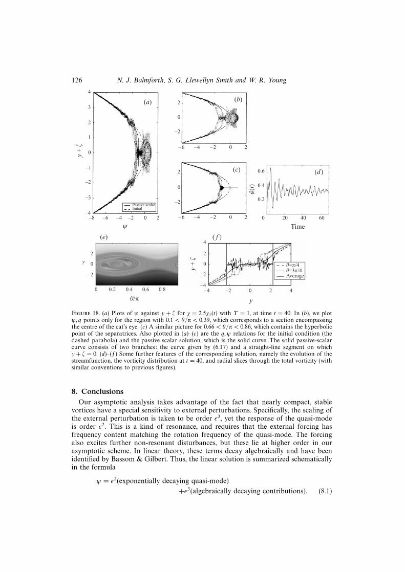
126 N. J. Balmforth, S. G. Llewellyn Smith and W. R. Young
4
3
2
1
0
–1
–2
–3
–4–8 –6 –4 –2 0 2
2
0
–2
–6 –4 –2 0 2
2
0
–2
–6 –4 –2 0 2
0.6
0.4
0.2
0 20 40 60
Passive scalarInitial
(a) (b)
(c) (d )
y +
ζ
Timeψ
(e)
2
0
–2
0 0.2 0.4 0.6 0.8
θ/π
4
2
0
–2
–4–4 –2 0 2 4
θ=π/4θ=3π/4Average
( f )
y
y
y +
ζ
Figure 18. (a) Plots of ψ against y + ζ for χ = 2.5χ1(t) with T = 1, at time t = 40. In (b), we plotψ, q points only for the region with 0.1 < θ/π < 0.39, which corresponds to a section encompassingthe centre of the cat’s eye. (c) A similar picture for 0.66 < θ/π < 0.86, which contains the hyperbolicpoint of the separatrices. Also plotted in (a)–(c) are the q, ψ relations for the initial condition (thedashed parabola) and the passive scalar solution, which is the solid curve. The solid passive-scalarcurve consists of two branches: the curve given by (6.17) and a straight-line segment on whichy + ζ = 0. (d)–(f) Some further features of the corresponding solution, namely the evolution of thestreamfunction, the vorticity distribution at t = 40, and radial slices through the total vorticity (withsimilar conventions to previous figures).
8. ConclusionsOur asymptotic analysis takes advantage of the fact that nearly compact, stable
vortices have a special sensitivity to external perturbations. Specifically, the scaling ofthe external perturbation is taken to be order ε3, yet the response of the quasi-modeis order ε2. This is a kind of resonance, and requires that the external forcing hasfrequency content matching the rotation frequency of the quasi-mode. The forcingalso excites further non-resonant disturbances, but these lie at higher order in ourasymptotic scheme. In linear theory, these terms decay algebraically and have beenidentified by Bassom & Gilbert. Thus, the linear solution is summarized schematicallyin the formula
ψ = ε2(exponentially decaying quasi-mode)
+ε3(algebraically decaying contributions). (8.1)

Disturbing vortices 127
p = 0 p = 1 p = 2
ω2/Zmax 1/4 0.185 0.158
r2/RC
√2 1.162 1.027
RCZmaxI1 16√
2 = 22.63 38.45 63.23
|I5|/RC 4√
2 = 5.657 4.647 4.107
γ/Zmax π√
2/16Υ = 0.278Υ 0.2205 Υ 0.1571 Υνc − 1 Υ 2Ac 1.187 Υ 2Ac 1.027 Υ 2Ac
Table 2. Numerical values of ω2, r2, and of the integrals I1 and I5 in (3.23) for the first threemembers (p = 0, 1 and 2) of the compact family in (2.3). The Landau damping rate, γ in (5.6),and the critical threshold of initial aspect ratio, νc in (C 5) are also shown. The nondimensionalparameter Υ ≡ RC|εZ ′S(r2)|/Zmax measures the strength of the perturbation relative to the underlyingcompact vortex. Using figure 13, our best estimate of Ac in the bottom row of the table is Ac ≈ 0.9.
Consequently, there is a switch-over from an initial exponential decay to a muchslower algebraic decay for times of order log(1/ε). The computations in Schecter etal. (1999) and Schecter (1999) display this exchange of order. We can summarize thelinear theory by saying that in almost all circumstances axisymmetrization occurs.Exceptions to the previous statement are provided by vortices which for one reason oranother possess undamped Kelvin modes. Into this category fall all contour dynamicalsimulations which employ discontinuous vorticity profiles.
The effect of nonlinearity is to slow the decay of the quasi-mode, or even arrest thatdecay if the initial amplitude of excitation exceeds a threshold. Above the threshold,cat’s eye structures form, and, in the case of an m = 2 perturbation, the result isa tripolar vortex, as seen in experiments. Because the forcing is scaled to be orderε3, this threshold is actually small. Thus, finite-amplitude cat’s eyes are the genericoutcome of resonantly exciting the quasi-mode of the vortex.
We now use the family of compact vortices defined in (2.3) to estimate the di-mensional Landau damping rate and the critical forcing threshold for the Gaussianvortex ZG = Zmax exp (−r2/R2
G). To ensure that the compact approximant has thesame circulation as the Gaussian vortex, we use the relation (2.6) to determine RC.The Landau damping rate, γ, is given in (5.6), and has the form of the dimen-sionless skirt vorticity gradient evaluated at the critical layer, Υ ≡ RC|εZ ′S|/Zmax,multiplying a profile-dependent numerical coefficient, which is given in table 2. Forthe Gaussian, Υ = 2
√2e−2, 0.3125 and 0.2608 for p = 0, 1 and 2, respectively. Hence,
γ/Zmax ≈ 0.1063, 0.069 and 0.041 in the three cases. This should be compared with thenumerical result for the Gaussian presented by Schecter et al. (1999): γ/Zmax ≈ 0.079.The damping rate for the case p = 0 is known analytically, namely γ/Zmax = (π e−2/4),and coincides with an earlier perturbation result quoted by Schecter et al. (1999). Thisagreement is rough, and surprisingly, the p = 1 vortex gives a better estimate thanp = 2.
To express the critical threshold in a more useful form, we specialize to instan-taneous kicks and convert Ac(T = 0) ≈ 0.9 into a critical initial aspect ratio ofthe perturbed vortex, as described in Appendix C. A perturbed vortex whose initialaspect ratio is greater than νc will not return to axisymmetry. Instead, the nonlinearterms result in the formation of a permanent cat’s eye structure. In Appendix C,we find that νc − 1 ∝ Υ 2, with numerical constants of proportionality as given intable 2. Again, for the Gaussian, we have νc − 1 ≈ 0.1318, 0.1043, 0.0625 for thethree values p = 0, 1 and 2. These estimates indicate that, without viscosity, 5 or

128 N. J. Balmforth, S. G. Llewellyn Smith and W. R. Young
10% departures from axisymmetry are sufficient to prevent axisymmetrization of anelliptical Gaussian vortex.
We expect that the reduced system (3.35)–(3.37) is broadly applicable as a modelof linear and weakly nonlinear relaxation in ideal plasmas and fluid shear flows. Inanalogy with plasma physics, one might call this system the ‘single-wave model’.
The view here is that if ε is small, so that a vortex is approximated by a compactvortex, then the single-wave model describes the weakly nonlinear evolution of themost easily excited perturbations on this vortex. Moreover for a certain class ofm = 2 perturbations we have calculated the critical initial aspect ratio for return toaxisymmetry.
This work was supported by the National Science Foundation (grant numberOCE9529 824), and partly carried out at the 1999 Geophysical Fluid Dynamics Sum-mer Study Program, Woods Hole Oceanographic Institution. S. G. L. S. was supportedby a Research Fellowship from Queens’ College. N. J. B. acknowledges an equipmentgrant from the Nuffield Foundation. We thank A. Bernoff and the anonymous refereesfor helping to improve the manuscript.
Appendix A. Computational technicalitiesWhen written in terms of F = ζ + βy, the equation for ζ reduces to the advection-
diffusion equation Ft+yFθ +ϕθFy = 0. (F can be used instead of ζ interchangeably inthe 〈 〉 term since 〈y〉 = 0.) We solve the equations with an operator splitting schemebased on the algorithm developed by Cheng & Knorr (1976) for the Vlasov equation(see also Feix et al. 1994), and subject to the boundary condition in y: ζ → 0 asy → ±∞. In order to save computing the evolution of unneeded angular harmonics,we consider a periodicity in θ of π rather than 2π.
A.1. Asymptotic solutions for large y
To avoid dealing with an infinite domain, we truncate the range in y and solve thevorticity equation over the region −L < y < L. This requires boundary conditionsat y = ±L. To increase the accuracy of this truncation of the domain, we use theasymptotic solution for large y: to order L−3,
ζ ∼ ζa = −ϕy
+1
2y2[χ(0)e2i(θ−yt) + c.c.]− 1
4y2ϕtθ. (A 1)
The slow algebraic decay of the vorticity complicates the numerical scheme over theoriginal Cheng & Knorr algorithm.
A.2. Operator splitting
We divide an integration step over the interval [t, t+ τ] into three stages:
A.2.1. Advect in θ for half a time step
This amounts to solving
Ft + yFθ = 0 (A 2)
over [t, t+τ/2], leaving ϕ unchanged. The exact solution is Fα(y, θ) = F(y, θ−yτ/2, t).This shift in θ is computed using Fourier interpolation.

Disturbing vortices 129
A.2.2. Advect in y for a complete time step
We then solve
Ft − 4(ϕr sin 2θ − ϕi cos 2θ)Fy = 0 (A 3)
and
iϕt = χ+ 〈e−2iθF〉 (A 4)
for [t, t+ τ], where ϕ(t) = ϕr(t) + iϕi(t). Because the advection in y amounts to a shiftof that coordinate, the integral in 〈e−2iθF〉 does not change during y-advection. Hencewe can deal with the equation for ϕ independently of the abridged vorticity equation.We do this by explicitly isolating the part of the integral over the computationaldomain, −L < y < L, from the part that originates outside. We approximate thelatter using the large-y theory (Haynes 1985). Hence,
〈e−2iθF〉 = 〈e−2iθF〉L − i
Lϕt +
1
Lχ(0)F(2Lt) + O(L−2), (A 5)
where
F(X) =
∫ ∞1
cos (Xη)dη
η2, (A 6)
and 〈 〉L has the obvious meaning. Hence,
i(1 + L−1)ϕt = χ+ 〈e−2iθF〉L +1
Lχ(0)F(2Lt) + O(L−2). (A 7)
But 〈e−2iθF〉L is constant over the step, and so
i(1 + L−1)[ϕ(t+ τ)− ϕ(t)]
= τ〈e−2iθF〉L +
∫ t+τ
t
[χ(s) +
1
Lχ(0)F(2Ls)
]ds+ O(τL−2). (A 8)
Now we solve the y-advection equation: Fβ(y, θ) = Fα(y − Vτ, θ), where V =−4(ϕr sin 2θ − ϕi cos 2θ), and ϕr = [ϕr(t+ τ) + ϕr(t)]/2 and ϕi = [ϕi(t+ τ) + ϕi(t)]/2are averages over the step. The introduction of these averages ensures second-orderaccuracy in time.
We accomplish the shift in y using interpolation with cubic splines. (Cubic splinesare also used to compute the integrals in 〈e−2iθF〉L.) The interpolation can be per-formed as long as the shifted position, −Vτ, lies inside the computational domain.However, for the boundary points, −L − Vτ lies below the domain if V > 0, andL−Vτ is above if V < 0. At these locations, we cannot use interpolation; the physicalsignificance is that fluid is being advected into the domain from outside. Instead wefix the values of F = ζ + βy at these points according to the solution for large |y| in(A 1).
A.2.3. Advect in θ for another half time step
Finally, we again advect in θ. This gives F(y, θ, t+ τ) = Fβ(y, θ − yτ/2) as the newvorticity distribution. Except at the first and final time steps, we can combine thisstep with the first one and shift in θ only once per time step.
A.3. Choice of time step
The main practical limitation on the time step (other than τ 1 for the sake ofprecision) is that we cannot shift in y over more than one grid point. Otherwise, fluid

130 N. J. Balmforth, S. G. Llewellyn Smith and W. R. Young
from outside invades our computational domain beyond one mesh point. Whilst thiscould easily be taken into account by using the asymptotic solution at the infectedgrid points, it signifies that accuracy is likely to be affected if the invasion becomessubstantial. To avoid this situation, we limit the time step to ensure that shifts overmore than one grid point do not take place.
With this limitation,
∆y > τVmax ≡ 4τ|ϕ|, (A 9)
where ∆y is the grid size in y. This leads us to choose a variable time step,
τ(t) = Min
[3∆y
16|ϕ(t)| , τmax
], (A 10)
where the arbitrary factor of 3/4 ensures we do not violate (A 9), and the upper limit,τmax, ensures we do not take an excessively long step. Note that there is no attemptto limit the amount of advection in θ.
In practice, for low-amplitude or short runs, we take τmax = 5 × 10⁻³. In longerruns with large-amplitude streamfunctions, we take τmax as low as 10−4 to improveprecision.
A.4. Further details
We have used various tests (doubling the grid size or maximum time step) to assessthe accuracy of the scheme. Based on these tests, we used the following recipe. Wechoose a computational grid of size (N, 2M + 1) to cover the interval 0 6 θ 6 πand −L 6 y 6 L. We use L = 5 or 10, N = 512 and M = 2000 or 4000 for thelarge-amplitude runs in which we study the cat’s eyes. For the lower-amplitude runsin which we compute the first bounce time, we use L = 10, N = 32 and M = 4000.
Spatial resolution is ultimately inadequate because of the increasing crenellation ofthe vorticity distribution. The finite resolution provides a numerical smoothing of thesolution by which small-scale structure is lost, as shown by the comparison of exactand numerical solutions in figure 7.
The main effect of the finite L is to introduce spurious, low-amplitude oscillationsinto the streamfunction. These are evident in the two panels of figure 5, and obscurethe ultimate decay of ϕ(t) in the cases in which cat’s eyes do not form. The frequencyand amplitude of the oscillations is determined by L and the magnitude of χ′(0); weattempted to choose L to minimize any effect of this spurious ringing, whilst retainingadequate spatial resolution.
Appendix B. The correction ϕ1(t) to the strongly forced limitThe expression (6.5) is obtained by multiplying the vorticity equation by y, spatially
averaging and integrating in time. In the notation of § 6.2, the resulting integral is
ϕ1(t) = 12〈yζ0(θ, y, t)〉 =
1
2
∫ ∞−∞
dy
∮dθ
2πy[y0(ξ, y, t)− y]. (B 1)
By symmetry, we need only consider y > 0 and −π/2 < ξ < π/2. The separatrixm = 1 divides the flow into two regions: one inside the cat’s eye with m > 1 and oneoutside with m < 1.
Outside the cat’s eye, we change variables from (ξ, y) to (u, m) where
sin ξ = sn(u;m), y =2√m
dn(u;m) (B 2)

Disturbing vortices 131
and
m =4
y2 + 4 sin2 ξ. (B 3)
The Jacobian of this transformation is ∂(ξ, y)/∂(u, m) = −2m−3/2. The range ofintegration becomes 0 < m < 1 and −K(m) < u < K(m), so the resulting subintegralis
I1 =8
π
∫ 1
0
dm
m5/2
∫ K(m)
−K(m)
dn(u;m)[ dn(u0;m)− dn(u;m)] du, (B 4)
where u0 = u− 2t/√m. The orientation of the mapping (ξ, y)→ (u, m) has been used
to obtain the correct sign of I1.
Now dn(u, m) may be expanded using
dn(u, m) =π
K(m)
[1
2+ 2
∞∑n=1
$n
1 + $2ncos (nπu/K)
](B 5)
and substituted into I1. The quantity
$(m) ≡ exp
[−πK(1− m)
K(m)
](B 6)
(usually denoted by q) is known as the nome. Orthogonality of trigonometric functionsleads to the result
I1 = −32π
∫ 1
0
dm
m5/2K(m)
∞∑n=1
$2n
(1 + $2n)2
1− cos
[2πnt√mK(m)
]. (B 7)
Inside the cat’s eye, Jacobi’s transformation may be used to transform from (ξ, y)to (v, m) by
sin ξ =1√m
sn(v;m−1), y =2√m
cn(v;m−1), (B 8)
which leads to ∂(ξ, y)/∂(v, m) = −2m−2. This mapping has negative orientation andthe resulting subintegral is
I2 = −8
π
∫ ∞1
dm
m3
∫ K(m−1)
−K(m−1)
cn(v;m−1)[ cn(v0;m−1)− cn(v;m−1)] dv, (B 9)
where v0 = v − 2t. The appropriate series to use now is
cn(v, 1/m) =2π√m
K(m−1)
∞∑n=1
$n−1/2
1 + $2n−1cos
[(n+ 1/2)πv
K(m−1)
]. (B 10)
Noting that $(m) = $(m−1) and using orthogonality leads to
I2 = 32π
∫ ∞1
dm
m2K(m−1)
∞∑n=1
$2n+1
(1 + $2n+1)2
1− cos
[(2n+ 1)πt
K(m−1)
]. (B 11)
Invoking the transformation K(m) = K(m−1)/√m and taking I1 + I2 gives (6.3).

132 N. J. Balmforth, S. G. Llewellyn Smith and W. R. Young
Appendix C. The initial aspect ratioFor an impulsive kick with real amplitude B, the external forcing function in (3.5)
is
ψext = 2r2Bδ(τ) cos 2ϑ, b(τ) = Bδ(τ) . (C 1)
The initial vorticity perturbation created by this kick is obtained from the balance
ζτ =1
r[Z ′C + εZ ′S]ψext
θ = −4rB[Z ′C + εZ ′S]δ(τ) sin 2ϑ (C 2)
in (3.3). Hence, at t = 0+, the total vorticity field is
ζTotal(r, θ, 0+) = [ZC(r) + εZS(r)]− 4ε2rB sin 2ϑ[ZC(r) + εZS(r)]′ + O(ε3)
≡ ZC(κ) + εZS(κ) + O(ε3), (C 3)
where κ = r−4ε2rB sin 2ϑ. The impulsive kick therefore deforms the vortex ellipticallyand the ratio of major and minor axes is given by
ν =1 + 4ε2|B|1− 4ε2|B| ≈ 1 + 8ε2|B|. (C 4)
We can relate B and A through the third relation in (3.34), and so
ν = 1 + 8ε2I1r2LA|I5|T . (C 5)
The final line in table 2 is calculated using (C 5) after evaluating I1 and I5. Todetermine the critical aspect ratio from the calculations in § 7 we take the limit T → 0so that χ→ Aδ(t). This corresponds to extrapolating the curves in figure 13 to T = 0,which gives Ac ≈ 0.9.
REFERENCES
Abramowitz, M. & Stegun, I. 1972 Handbook of Mathematical Functions. Dover.
Balmforth, N. J. 1998 Stability of vorticity defects in viscous shear. J. Fluid Mech. 357, 199–224.
Balmforth, N. J., del-Castillo-Negrete, D. & Young, W. R. 1997 Dynamics of vorticity defectsin shear. J. Fluid Mech. 333, 197–230.
Bassom, A. P. & Gilbert, A. D. 1998 The spiral wind-up of vorticity in an inviscid planar vortex.J. Fluid Mech. 371, 109–140.
Batchelor, G. K. 1967 An Introduction to Fluid Dynamics. Cambridge University Press.
Benney, D. J. & Bergeron, R. F. 1969 A new class of nonlinear waves in parallel flows. Stud. Appl.Maths 48, 181–204.
Bernoff, A. J. & Lingevitch, J. 1994 Rapid relaxation of an axisymmetrical vortex. Phys. Fluids6, 3717–3723.
Bernstein, I. B., Greene, J. M. & Kruskal, M. D. 1958 Exact nonlinear plasma oscillations. Phys.Rev. 108, 546–550.
Briggs, R. J., Daugherty, J. D. & Levy, R. H. 1970 Role of Landau damping in crossed-fieldelectron beams and inviscid shear flows. Phys. Fluids 13, 421–432.
Cass, A. C. 1998 Experiments on Vortex Symmetrization in magnetized electron plasma columns.PhD thesis, University of California, San Diego.
Cheng, C. Z. & Knorr, G. 1976 The integration of the Vlasov equation in configuration space.J. Comput. Phys. 22, 330–351.
Churilov, S. M. & Shukhman, I. G. 1987 The nonlinear development of disturbances in a zonalshear flow. Geophys. Astrophys. Fluid Dyn. 38, 145–175.
del-Castillo-Negrete, D. 1998 Weakly nonlinear dynamics of electrostatic perturbations inmarginally stable plasmas. Phys. Plasmas 5, 3886–3900.

Disturbing vortices 133
Driscoll, C. F. & Fine, F. S. 1990 Experiments on vortex dynamics in pure electron plasma. Phys.Fluids B 2, 1359–1366.
Dritschel, D. G. 1998 On the persistence of non-axisymmetric vortices in inviscid two-dimensionalflows. J. Fluid Mech. 371, 141–155.
Feix, M. R., Bertrand, P. & Ghizzo, A. 1994 Eulerian codes for the Vlasov equation. In Advancesin Kinetic Theory and Computing (ed. B. Perthame), pp. 45–81. World Scientific.
Goldstein, M. E. & Hultgren, L. S. 1988 Nonlinear spatial evolution of an externally excitedinstability wave in a free shear layer. J. Fluid Mech. 197, 259–330.
Goldstein, M. E. & Leib, S. J. 1988 Nonlinear roll-up of externally excited free shear layers. J. FluidMech. 191, 481–515.
Gould, R. W. 1994 Dynamics of non-neutral plasmas. Phys. Plasmas 2, 2151–2163.
Haynes, P.H. 1985 Nonlinear instability of a Rossby-wave critical layer. J. Fluid Mech. 161, 493–511.
Heijst, G. J. F. van, Kloosterziel, R. C. & Williams, C. W. M. 1991 Laboratory experiments onthe tripolar vortex in a rotating fluid. J. Fluid Mech. 225, 301–331.
Imamura, T., Sugihara, R. & Taniuti, T. 1969 An asymptotic method for the Vlasov equation.J. Phys. Soc. Japan 27, 1623–1630.
Kelvin, Lord 1880 On the vibrations of a columnar vortex. Phil. Mag. 10, 155–168.
Killworth, P. D. & McIntyre, M. E. 1985 Do Rossby-wave critical layers absorb, reflect orover-reflect? J. Fluid Mech. 161, 449–492.
Kloosterziel, R. C. & Carnevale, G. F. 1999 On the evolution and saturation of instabilities oftwo-dimensional isolated circular vortices. J. Fluid Mech. 388, 217–257.
Le Dizes, S. 2000 Non-axisymmetric vortices in two-dimensional flows. J. Fluid Mech. 406, 175–198.
Lingevitch, J. F. & Bernoff, A. J. 1995 Distortion and evolution of a localized vortex in anirrotational flow. Phys. Fluids 7, 1015–1026.
Manfredi, G. 1997 Long-time behaviour of nonlinear Landau damping. Phys. Rev. Lett. 79, 2815–2819.
Moller, J. D. & Montgomery, M. T. 1999 Vortex Rossby waves and hurricane intensification ina barotropic model. J. Atmos. Sci. 56, 1674–1687.
Montgomery, M. T. & Kallenbach, R. J. 1997 A theory for vortex Rossby waves and its applicationto spiral bands and intensity changes in hurricanes. Q. J. R. Met. Soc. 123, 435–465.
O’Neil, T. M. 1965 Collisionless damping of nonlinear plasma oscillations. Phys. Fluids 8, 2255–2262.
O’Neil, T. M.,Winfrey, J. H. & Malmberg, J. H. 1971 Nonlinear interaction of a small cold beamand a plasma. Phys. Fluids 14, 1204–1212.
Rayleigh, Lord 1880 On the stability, or instability, of certain fluid motions. Proc. Lond. Math.Soc. 9, 57–70.
Rhines, P. B. & Young, W. R. 1983 How rapidly is passive scalar mixed within closed streamlines?J. Fluid Mech. 133, 133–145.
Rossi, L. F., Lingevitch, J. F. & Bernoff, A. J. 1997 Quasi-steady monopole and tripole attractorsfor relaxing vortices. Phys. Fluids 9, 2329-2338.
Schecter, D. A. 1999 On the dynamics of inviscid relaxation in 2D fluids and nonneutral plasmas.PhD thesis, University of California, San Diego.
Schecter, D. A., Dubin, D. H. E., Cass, A. C., Driscoll, C. F., Lansky, I. M. & O’Neil, T. M. 1999Inviscid damping of elliptical perturbations on a 2D vortex. In AIP Proc. 1999 Non-neutralPlasmas Workshop.
Stewartson, K. 1978 The evolution of the critical layer of a Rossby wave. Geophys. Astrophys.Fluid Dyn. 9, 185–200.
Stewartson, K. 1981 Marginally stable inviscid flows with critical layers. IMA J. Appl. Maths 27,133–175.
Sugihara, R. & Kamimura, T. 1972 An asymptotic method for the Vlasov equation. III Transitionfrom amplitude oscillations to linear Landau damping. J. Phys. Soc. Japan 33, 206–215.
Tennyson, J. L., Meiss, J. D. & Morrison, P. J. 1994 Self-consistent chaos in the beam-plasmainstability. Physica D 71, 1–17.
Warn, T. & Gauthier, P. 1989 Potential vorticity mixing by marginally unstable baroclinic distur-bances. Tellus 41A, 115–131.
Warn, T. & Warn, H. 1978 The evolution of a nonlinear critical level. Stud. Appl. Maths 59, 37–71.


