Distributionally Robust Optimization with In nitely ... · Chen, Sim, and Xu: Distributionally...
41
manuscript Distributionally Robust Optimization with Infinitely Constrained Ambiguity Sets Zhi Chen Imperial College Business School, Imperial College London [email protected] Melvyn Sim Department of Analytics & Operations, NUS Business School, National University of Singapore [email protected] Huan Xu H. Milton Stewart School of Industrial and Systems Engineering, Georgia Institute of Technology [email protected] We consider a distributionally robust optimization problem where the ambiguity set of probability distri- butions is characterized by a tractable conic representable support set and by expectation constraints. We propose a new class of infinitely constrained ambiguity sets for which the number of expectation constraints could be infinite. The description of such ambiguity sets can incorporate the stochastic dominance, dis- persion, fourth moment, and our newly proposed “entropic dominance” information about the uncertainty. In particular, we demonstrate that including this entropic dominance can improve the characterization of stochastic independence as compared with a characterization based solely on covariance information. Because the corresponding distributionally robust optimization problem need not lead to tractable reformulations, we adopt a greedy improvement procedure that consists of solving a sequence of tractable distributionally robust optimization subproblems—each of which considers a relaxed and finitely constrained ambiguity set. Our computational study establishes that this approach converges reasonably well. Key words : distributionally robust optimization; stochastic programming; entropic dominance. History : May 20, 2018. 1. Introduction In recent years, distributionally robust optimization has become a popular approach for addressing optimization problems contaminated by uncertainty. The attractive features of distributionally robust optimization include not only its flexibility in the specification of uncertainty beyond a fixed probability distribution but also its ability to yield computationally tractable models. Its idea can be traced back to minimax stochastic programming, in which optimal solutions are evaluated under the worst-case expectation in response to a family of probability distributions of uncertain parameters (see, for instance, Scarf 1958, Dupaˇ cov´ a 1987, Gilboa and Schmeidler 1989, Breton and El Hachem 1995, Shapiro and Kleywegt 2002). 1
Transcript of Distributionally Robust Optimization with In nitely ... · Chen, Sim, and Xu: Distributionally...

manuscript
Distributionally Robust Optimizationwith Infinitely Constrained Ambiguity Sets
Zhi ChenImperial College Business School, Imperial College London
Melvyn SimDepartment of Analytics & Operations, NUS Business School, National University of Singapore
Huan XuH. Milton Stewart School of Industrial and Systems Engineering, Georgia Institute of Technology
We consider a distributionally robust optimization problem where the ambiguity set of probability distri-
butions is characterized by a tractable conic representable support set and by expectation constraints. We
propose a new class of infinitely constrained ambiguity sets for which the number of expectation constraints
could be infinite. The description of such ambiguity sets can incorporate the stochastic dominance, dis-
persion, fourth moment, and our newly proposed “entropic dominance” information about the uncertainty.
In particular, we demonstrate that including this entropic dominance can improve the characterization of
stochastic independence as compared with a characterization based solely on covariance information. Because
the corresponding distributionally robust optimization problem need not lead to tractable reformulations,
we adopt a greedy improvement procedure that consists of solving a sequence of tractable distributionally
robust optimization subproblems—each of which considers a relaxed and finitely constrained ambiguity set.
Our computational study establishes that this approach converges reasonably well.
Key words : distributionally robust optimization; stochastic programming; entropic dominance.
History : May 20, 2018.
1. Introduction
In recent years, distributionally robust optimization has become a popular approach for addressing
optimization problems contaminated by uncertainty. The attractive features of distributionally
robust optimization include not only its flexibility in the specification of uncertainty beyond a
fixed probability distribution but also its ability to yield computationally tractable models. Its idea
can be traced back to minimax stochastic programming, in which optimal solutions are evaluated
under the worst-case expectation in response to a family of probability distributions of uncertain
parameters (see, for instance, Scarf 1958, Dupacova 1987, Gilboa and Schmeidler 1989, Breton and
El Hachem 1995, Shapiro and Kleywegt 2002).
1
Chen, Sim, and Xu: Distributionally Robust Optimization with Infinitely Constrained Ambiguity Sets
2
The problem usually studied in distributionally robust optimization is as follows:
minx∈X
supP∈F
EP [f(x, z)] , (1)
where x ∈ X ⊆ RM is the “here-and-now” decision taken before the uncertainty realizes, z ∈ RN
is the realization of that uncertainty, and f(·, ·) : X ×RN 7→R is the objective function. Given the
decision x, the distributionally robust optimization model (1) evaluates the worst-case expected
objective
ρ(x) = supP∈F
EP [f(x, z)] (2)
with reference to the ambiguity set, denoted by F . Distributionally robust optimization is a true
generalization of classical robust optimization and stochastic programming. When the ambiguity
set contains only the support information—that is, when F = {P∈P0(RN) | z ∼ P, P [z ∈W] = 1},
the evaluation criterion (2) reduces to the worst-case objective
ρ(x) = supz∈W
f(x,z)
as in classical robust optimization (see, for instance, Soyster 1973, Ben-Tal and Nemirovski 1998,
El Ghaoui et al. 1998, Bertsimas and Sim 2004). When the ambiguity set is a singleton (i.e.,
F = {P0}), the evaluation criterion (2) recovers the expected objective
ρ(x) =EP0 [f(x, z)]
considered in stochastic programming (see, for instance, Birge and Louveaux 2011).
The introduction of an ambiguity set leads to greater modeling power and allows us to incor-
porate information about the uncertainty, such as support and descriptive statistics (e.g., mean,
moments, and dispersions; see El Ghaoui et al. 2003, Chen et al. 2007, Chen and Sim 2009, Delage
and Ye 2010, Wiesemann et al. 2014, Hanasusanto et al. 2017). Recent studies have led to signifi-
cant progress on computationally tractable reformulations for distributionally robust optimization,
which is closely related to the interplay between the ambiguity set and the objective function.
In particular, Delage and Ye (2010) propose tractable reformulations for distributionally robust
optimization problems, in which the ambiguity set is specified by the first and second moments
that themselves could be uncertain. Wiesemann et al. (2014) propose a broad class of ambiguity
sets with conic representable expectation constraints and a collection of nested conic representable
confidence sets. The authors identify conditions under which the distributionally robust optimiza-
tion problem has an explicit tractable reformulation. They also comment that from the theoretical
standpoint, an optimization problem is considered tractable if it can be solved in polynomial time;
yet for practical applications of general interest, the problem is tractable only when formatted as

Chen, Sim, and Xu: Distributionally Robust Optimization with Infinitely Constrained Ambiguity Sets
3
a linear or second-order conic program, or, to a lesser degree, a semidefinite program. Another
popular type of ambiguity sets is based on limiting the statistical distance (in terms of certain
statistical distance measure) of their members to a reference probability distribution. Through the
choice of the statistical distance measure, examples of the statistical-distance-based ambiguity sets
include the φ-divergence ambiguity set (Ben-Tal et al. 2013, Jiang and Guan 2016, Wang et al.
2016) and the Wasserstein ambiguity set (Pflug and Wozabal 2007, Gao and Kleywegt 2016, Esfa-
hani and Kuhn 2017, Zhao and Guan 2018). More recently, as shown in Chen et al. (2017), these
ambiguity sets can be characterized by a finite number of expectation constraints and they belong
to the type of scenario-wise ambiguity sets with (conditional) expectation constraints based on
generalized moments. While these ambiguity sets lead to tractable reformulations, they may not
be able to capture important distributional information such as stochastic independence, which is
ubiquitous in characterizing uncertainty.
In this paper, we proposed a new class of ambiguity set that encompasses a potentially infinite
number of expectation constraints, which has the benefits of, among other things, tightening the
approximation of ambiguity sets with information on stochastic independence. We call this class
the infinitely constrained ambiguity set, which is complementary to existing ambiguity sets in the
literature such as the one in Wiesemann et al. (2014). Although the corresponding distributionally
robust optimization problem may not generally lead to tractable reformulations, we propose an
algorithm involving a greedy improvement procedure to solve the problem. In each iteration, the
algorithm yields a monotonic improvement over the previous solution. Our computational study
reveals that this approach converges reasonably well.
The paper’s main contributions can be summarized as follows.
1. We propose a new class of infinitely constrained ambiguity sets that would allow ambiguous
probability distributions to be characterized by an infinite number of expectation constraints, which
can be naturally integrated into existing ambiguity sets. We elucidate the generality of this class
for characterizing distributional ambiguity when addressing distributionally robust optimization
problems. We also present several examples of infinitely constrained ambiguity sets.
2. To solve the corresponding distributionally robust optimization problem, we propose a greedy
improvement procedure to obtain its solution by solving a sequence of subproblems. Each of these
subproblems is a tractable distributionally robust optimization problem, in which the ambiguity
set is finitely constrained and is a relaxation of the infinitely constrained ambiguity set. At each
iteration, we also solve a separation problem that enables us to obtain a tighter relaxation and
thus a monotonic improvement over the previous solution.
3. When incorporating covariance and fourth moment information into the ambiguity set, we
show that the subproblems are second-order conic programs. This differs from the literature where
Chen, Sim, and Xu: Distributionally Robust Optimization with Infinitely Constrained Ambiguity Sets
4
the distributionally robust optimization problem with an ambiguity set involving only covariance
information is usually reformulated as a semidefinite program. An important advantage of having
a second-order conic optimization formulation is the availability of state-of-the-art commercial
solvers that also support discrete decision variables.
4. We introduce the entropic dominance ambiguity set : an infinitely constrained ambiguity set
that incorporates an upper bound on the uncertainty’s moment-generating function. This entropic
dominance can yield an improved characterization of stochastic independence than can be achieved
via the existing approach based solely on covariance information. Although the corresponding
separation problem is not convex, we show computationally that the trust region method works
well, and that we are able to obtain less conservative solutions if the underlying uncertainties are
independently distributed.
The rest of our paper proceeds as follows. We introduce and motivate the infinitely constrained
ambiguity set in Section 2. In Section 3, we study the corresponding distributionally robust opti-
mization problem and focus on relaxing the ambiguity set to obtain a tractable reformulation
for the worst-case expected objective; toward that end, we propose an algorithm to tighten the
relaxation. We address covariance and the fourth moment in Section 4 and Section 5 is devoted to
the entropic dominance; in these sections, we also demonstrate potential applications. Proofs not
included in the main text are given in the electronic companion.
Notation: Boldface uppercase and lowercase characters represent (respectively) matrices and vec-
tors, and [x]i or xi denotes the i-th element of the vector x. We denote the n-th standard unit basis
vector by en, the vector of 1s by e, ,the vector of 0s by 0, and the set of positive running indices up to
N by [N ] = {1,2, . . . ,N}. For a proper cone K∈RN , the set constraint y−x∈K is equivalent to the
general inequality x� y. We use K∗ to signify the dual cone of K such that K∗ = {y | y′x≥ 0,∀x∈
K}. We denote the second-order cone by KSOC, i.e., (a,b)∈KSOC refers to a second-order conic con-
straint ||b||2 ≤ a. For the exponential cone, we write KEXP = cl{
(d1, d2, d3) | d2 > 0, d2ed1/d2 ≤ d3
}and its dual cone by K∗EXP = cl
{(d1, d2, d3) | d1 < 0,−d1e
d2/d1 ≤ ed3
}. We denote the set of all Borel
probability distributions on RN by P0(RN). A random variable z is denoted with a tilde sign and
we use z ∼ P, P ∈ P0 (RN) to denote z as an N -dimensional random variable with probability
distribution P.
2. Infinitely constrained ambiguity set
Wiesemann et al. (2014) propose a class of conic representable ambiguity sets that results in
tractable reformulations of distributionally robust optimization problems with convex piecewise
Chen, Sim, and Xu: Distributionally Robust Optimization with Infinitely Constrained Ambiguity Sets
5
affine objective functions in the form of conic optimization problems. The following tractable conic
ambiguity set is an expressive example of the ambiguity set in Wiesemann et al. (2014).
FT =
P∈P0
(RN)∣∣∣∣∣∣∣∣∣∣∣
z ∼ P
EP [Gz] =µ
EP [g(z)]�K h
P [z ∈W] = 1
(3)
with parametersG∈RL×N , µ∈RL, and h∈RL1 and with functions g : RN 7→RL1 . The K-epigraph
of the function g, that is, {(z,u)∈RN ×RL1 | g(z)�K u}, is tractable conic representable via conic
inequalities involving tractable cones. The support set W is also tractable conic representable. We
refer readers to Ben-Tal and Nemirovski (2001) for an excellent introduction to conic representation
and we refer to the nonnegative orthant, second-order cone, exponential cone, positive semidefinite
cone, and their Cartesian product as the tractable cone.
In the tractable conic ambiguity set FT, the equality expectation constraint specifies the mean
values of Gz. At the same time, the conic inequality expectation constraint characterizes the dis-
tributional ambiguity via a bound on mean, covariance, expected utility, and others. Observe that
we can replace the conic inequality expectation constraint by a set of infinitely many expectation
constraints as follows:
FT =
P∈P0
(RN)∣∣∣∣∣∣∣∣∣∣∣
z ∼ P
EP [Gz] =µ
EP [q′g(z)]≤ q′h, ∀q ∈K∗
P [z ∈W] = 1
,
where K∗ is the dual cone of K.
In this paper, we propose the infinitely constrained ambiguity set—by extending the tractable
conic ambiguity set to incorporate a potentially infinite number of expectation constraints—as
follows:
FI =
P∈P0
(RN)∣∣∣∣∣∣∣∣∣∣∣
z ∼ P
EP [Gz] =µ
EP [gi(qi, z)]≤ hi(qi), ∀qi ∈Qi,∀i∈ [I]
P [z ∈W] = 1
; (4)
here sets Qi ⊆RMi , functions gi : Qi×RN 7→R, and functions hi : Qi 7→R for i ∈ [I]. The support
set W is bounded, nonempty, and tractable conic representable. We also assume that the epigraph
of the function gi(qi,z) is tractable conic representable with respect to z for any qi ∈Qi.
The generality of our infinitely constrained ambiguity set is elucidated in the following result.

Chen, Sim, and Xu: Distributionally Robust Optimization with Infinitely Constrained Ambiguity Sets
6
Theorem 1. Let X be any infinite set in the real space. Suppose that, for any x∈X , the function
f(x,z) : X ×RN 7→R is tractable conic representable in the variable z. Then for any ambiguity set
F ⊆P0 (RN) , there exists an infinitely constrained ambiguity set FI ⊆P0 (RN) such that
supP∈F
EP [f(x, z)] = supP∈FI
EP [f(x, z)] , ∀x∈X .
Proof. We consider the ambiguity set
FI =
P∈P0
(RN) ∣∣∣∣∣∣ z ∼ P
EP [g(q, z)]≤ h(q), ∀q ∈Q
,
where Q,X , h (q), supP∈F EP [f(q, z)], and g(q,z), f(q,z). Observe that the function g(q,z) is
tractable conic representable in z for any q ∈Q and that the set Q is infinite; hence the constructive
set FI is an infinitely constrained ambiguity set.
On the one hand, for any P∈FI we have
EP [f(x, z)] =EP [g(x, z)]≤ h(x) = supP∈F
EP [f(x, z)] , ∀x∈X ,
which implies that
supP∈FI
EP [f(x, z)]≤ supP∈F
EP [f(x, z)] , ∀x∈X .
On the other hand, for any P∈F we have
EP [g(x, z)] =EP [f(x, z)]≤ supP∈F
EP [f(x, z)] = h(x), ∀x∈X ;
hence P∈FI and F ⊆FI. As a result,
supP∈F
EP [f(x, z)]≤ supP∈FI
EP [f(x, z)] , ∀x∈X .
We can therefore conclude that
supP∈F
EP [f(x, z)] = supP∈FI
EP [f(x, z)] , ∀x∈X . �
Using Theorem 1, we can represent the distributionally robust optimization problem (1) with
any ambiguity set F as one with an infinitely constrained ambiguity set FI—provided the objective
function f(x,z) is tractable conic representable in z for any x ∈ X . This observation reveals the
generality of the infinitely constrained ambiguity set for characterizing distributional ambiguity in
distributionally robust optimization models. We emphasize that FI is not necessarily a substitution
of existing ambiguity sets but can also be naturally integrated with them: for any ambiguity set F ,
we can always consider an intersection F⋂FI, which shall inherit the modeling power from both
ambiguity sets. The infinitely constrained ambiguity set FI indeed enables us to characterize some
new properties of uncertain probability distributions. We now provide some examples.
Chen, Sim, and Xu: Distributionally Robust Optimization with Infinitely Constrained Ambiguity Sets
7
Stochastic dominance ambiguity set
Stochastic dominance, particularly in the second order, is a form of stochastic ordering that is
prevalent in decision theory and economics.
Definition 1. A random outcome z ∼ P dominates another random outcome z† ∼ P† in the
second order, written z �(2) z†, if EP [u(z)]≥ EP† [u(z†)] for every concave nondecreasing function
u(·), for which these expected values are finite.
The celebrated expected utility hypothesis, introduced by von Neumann and Morgenstern (1947),
states that: for every rational decision maker, there exists a utility function u(·) such that she
prefers the random outcome z over some random outcome z† if and only if EP [u(z)]>EP† [u(z†)]. In
practice, however, it is almost impossible for a decision maker to elicit her utility function. Instead,
Dentcheva and Ruszczynski (2003) propose a safe relaxation of the constraint EP [u(z)]>EP† [u(z†)]
by considering the second-order stochastic dominance constraint z �(2) z†. This constraint ensures
that, without articulating her utility function, the decision maker will prefer the payoff z over the
benchmark payoff z† as long as her utility function u(·) is concave and nondecreasing. The proposal
is practically useful in many applications. In portfolio optimization problems, for instance, one can
construct the reference portfolio from past return rates and then attempt to devise a more nearly
optimal portfolio under the constraint that it dominates the reference portfolio (see Dentcheva and
Ruszczynski 2006). The second-order stochastic dominance constraint z �(2) z† has an equivalent
representation
EP[(q− z)+]≤EP† [(q− z†)+], ∀q ∈R,
which can be readily incorporated into an infinitely constrained ambiguity set. In fact, the modeling
capability of that set extends to higher-order stochastic dominance relations; for more details, see
Dentcheva and Ruszczynski (2003).
Mean-dispersion ambiguity set
In the class of mean-dispersion ambiguity sets, probability distributions of the uncertainty are
characterized by the support and mean and by upper bounds on their dispersion. Mean-dispersion
ambiguity sets recover a range of ambiguity sets from the literature and have been recently studied
in Hanasusanto et al. (2017) for joint chance constraints. A typical mean-dispersion ambiguity set
FD satisfies
FD =
P∈P0
(RN)∣∣∣∣∣∣∣∣∣∣∣
z ∼ P
EP [z] =µ
EP [g(q, z)]≤ h(q), ∀q ∈Q
P [z ∈W] = 1
, (5)
Chen, Sim, and Xu: Distributionally Robust Optimization with Infinitely Constrained Ambiguity Sets
8
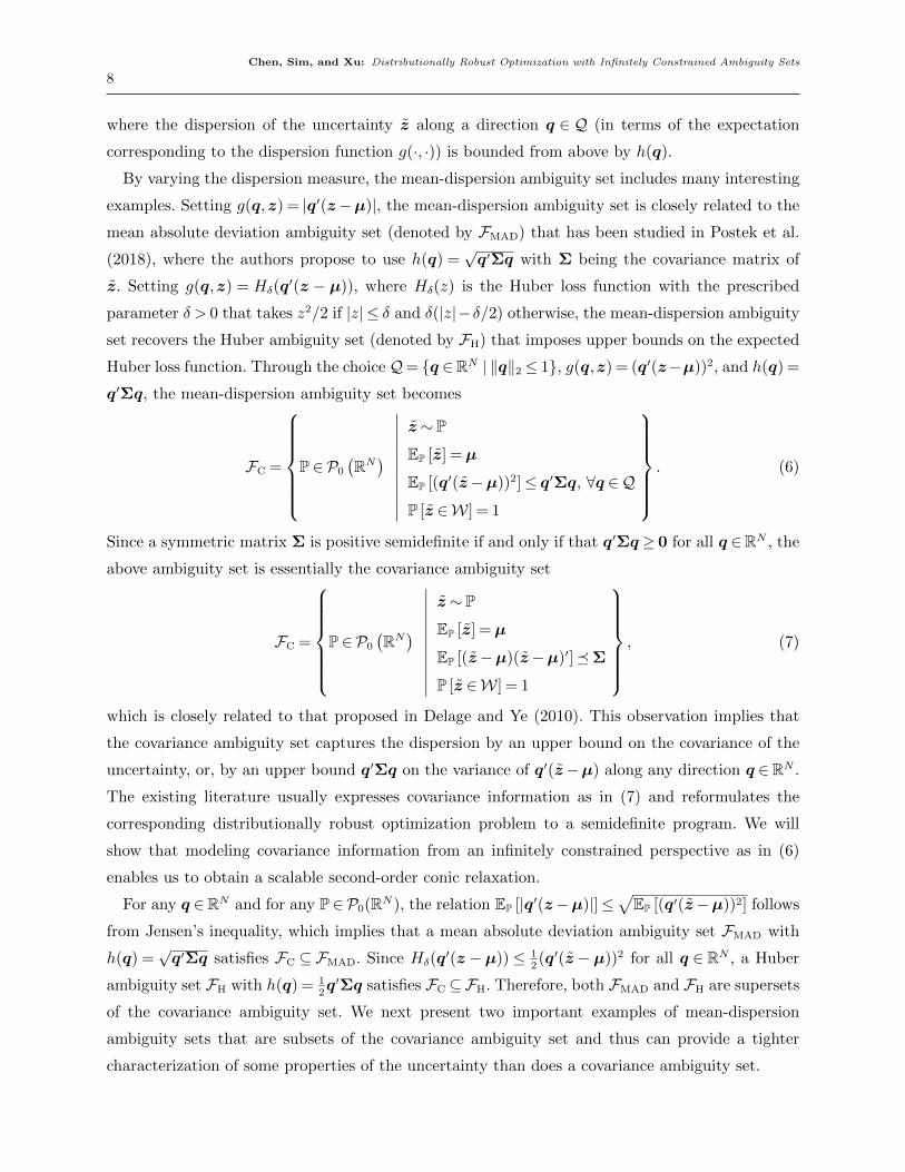
where the dispersion of the uncertainty z along a direction q ∈ Q (in terms of the expectation
corresponding to the dispersion function g(·, ·)) is bounded from above by h(q).
By varying the dispersion measure, the mean-dispersion ambiguity set includes many interesting
examples. Setting g(q,z) = |q′(z−µ)|, the mean-dispersion ambiguity set is closely related to the
mean absolute deviation ambiguity set (denoted by FMAD) that has been studied in Postek et al.
(2018), where the authors propose to use h(q) =√q′Σq with Σ being the covariance matrix of
z. Setting g(q,z) = Hδ(q′(z − µ)), where Hδ(z) is the Huber loss function with the prescribed
parameter δ > 0 that takes z2/2 if |z| ≤ δ and δ(|z|−δ/2) otherwise, the mean-dispersion ambiguity
set recovers the Huber ambiguity set (denoted by FH) that imposes upper bounds on the expected
Huber loss function. Through the choice Q= {q ∈RN | ‖q‖2 ≤ 1}, g(q,z) = (q′(z−µ))2, and h(q) =
q′Σq, the mean-dispersion ambiguity set becomes
FC =
P∈P0
(RN)∣∣∣∣∣∣∣∣∣∣∣
z ∼ P
EP [z] =µ
EP [(q′(z−µ))2]≤ q′Σq, ∀q ∈Q
P [z ∈W] = 1
. (6)
Since a symmetric matrix Σ is positive semidefinite if and only if that q′Σq≥ 0 for all q ∈RN , the
above ambiguity set is essentially the covariance ambiguity set
FC =
P∈P0
(RN)∣∣∣∣∣∣∣∣∣∣∣
z ∼ P
EP [z] =µ
EP [(z−µ)(z−µ)′]�Σ
P [z ∈W] = 1
, (7)
which is closely related to that proposed in Delage and Ye (2010). This observation implies that
the covariance ambiguity set captures the dispersion by an upper bound on the covariance of the
uncertainty, or, by an upper bound q′Σq on the variance of q′(z−µ) along any direction q ∈RN .
The existing literature usually expresses covariance information as in (7) and reformulates the
corresponding distributionally robust optimization problem to a semidefinite program. We will
show that modeling covariance information from an infinitely constrained perspective as in (6)
enables us to obtain a scalable second-order conic relaxation.
For any q ∈RN and for any P∈P0(RN), the relation EP [|q′(z−µ)|]≤√
EP [(q′(z−µ))2] follows
from Jensen’s inequality, which implies that a mean absolute deviation ambiguity set FMAD with
h(q) =√q′Σq satisfies FC ⊆ FMAD. Since Hδ(q
′(z −µ))≤ 12(q′(z −µ))2 for all q ∈ RN , a Huber
ambiguity set FH with h(q) = 12q′Σq satisfies FC ⊆FH. Therefore, both FMAD and FH are supersets
of the covariance ambiguity set. We next present two important examples of mean-dispersion
ambiguity sets that are subsets of the covariance ambiguity set and thus can provide a tighter
characterization of some properties of the uncertainty than does a covariance ambiguity set.
Chen, Sim, and Xu: Distributionally Robust Optimization with Infinitely Constrained Ambiguity Sets
9
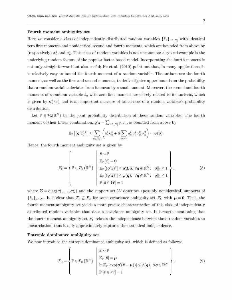
Fourth moment ambiguity set
Here we consider a class of independently distributed random variables {zn}n∈[N ] with identical
zero first moments and nonidentical second and fourth moments, which are bounded from above by
(respectively) σ2n and κ4
n. This class of random variables is not uncommon: a typical example is the
underlying random factors of the popular factor-based model. Incorporating the fourth moment is
not only straightforward but also useful; He et al. (2010) point out that, in many applications, it
is relatively easy to bound the fourth moment of a random variable. The authors use the fourth
moment, as well as the first and second moments, to derive tighter upper bounds on the probability
that a random variable deviates from its mean by a small amount. Moreover, the second and fourth
moments of a random variable zn with zero first moment are closely related to its kurtosis, which
is given by κ4n/σ
4n and is an important measure of tailed-ness of a random variable’s probability
distribution.
Let P ∈ P0(RN) be the joint probability distribution of these random variables. The fourth
moment of their linear combination, q′z =∑
n∈[N ] qnzn, is bounded from above by
EP[(q′z)4
]≤∑n∈[N ]
(q4nκ
4n + 6
∑m 6=n
q2mq
2nσ
2mσ
2n
)=ϕ(q).
Hence, the fourth moment ambiguity set is given by
FF =
P∈P0
(RN)∣∣∣∣∣∣∣∣∣∣∣∣∣∣
z ∼ P
EP [z] = 0
EP [(q′z)2]≤ q′Σq, ∀q ∈RN : ‖q‖2 ≤ 1
EP [(q′z)4]≤ϕ(q), ∀q ∈RN : ‖q‖2 ≤ 1
P [z ∈W] = 1
, (8)
where Σ = diag(σ21, . . . , σ
2N) and the support set W describes (possibly nonidentical) supports of
{zn}n∈[N ]. It is clear that FF ⊆ FC for some covariance ambiguity set FC with µ = 0. Thus, the
fourth moment ambiguity set yields a more precise characterization of this class of independently
distributed random variables than does a covariance ambiguity set. It is worth mentioning that
the fourth moment ambiguity set FF relaxes the independence between these random variables to
uncorrelation, thus it only approximately captures the statistical independence.
Entropic dominance ambiguity set
We now introduce the entropic dominance ambiguity set, which is defined as follows:
FE =
P∈P0
(RN)∣∣∣∣∣∣∣∣∣∣∣
z ∼ P
EP [z] =µ
lnEP [exp(q′(z−µ))]≤ φ(q), ∀q ∈RN
P [z ∈W] = 1
; (9)

Chen, Sim, and Xu: Distributionally Robust Optimization with Infinitely Constrained Ambiguity Sets
10
here φ : RN 7→R is some convex and twice continuously differentiable function that satisfies φ(0) = 0
and ∇φ(0) = 0 for ∇φ(·) the gradient of φ(·). The entropic dominance ambiguity set virtually
bounds from above the logged moment-generating function of the random variable z as adjusted
by its mean µ. Hence, the entropic dominance ambiguity set can encompass common random
variables used in statistics—such as sub-Gaussian (Wainwright 2015), a class of random variables
with exponentially decaying tails. A formal definition follows.
Definition 2. A random variable z with mean µ is sub-Gaussian with deviation parameter
σ > 0, if
lnEP [exp(q(z−µ))]≤ q2σ2
2, ∀q ∈R.
In the case of a normal distribution, the deviation parameter σ corresponds to the standard
deviation and we have equality in the relation just defined. So if {zn}n∈[N ] are independently dis-
tributed sub-Gaussian random variables with means {µn}n∈[N ] and deviation parameters {σn}n∈[N ],
then we can specify the entropic dominance ambiguity set (9) by letting φ(q) = 12
∑n∈[N ] q
2nσ
2n.
It is worth noting that the class of infinitely many expectation constraints implicitly specifies the
mean, an upper bound on the covariance, and a superset of the support of a probability distribution.
Theorem 2. For any probability distribution P that satisfies
lnEP [exp(q′(z−µ))]≤ φ(q), ∀q ∈RN ,
we have: EP [z] =µ, EP [(z−µ)(z−µ)′]�∇2φ(0), and
W ⊆{z ∈RN
∣∣∣ q′(z−µ)≤ limα→∞
1
αφ(αq), ∀q ∈RN
}.
If φ(q) has an additive form given by φ(q) =∑
n∈[N ] φn(qn), where φn(0) = 0 for all n ∈ [N ], then
we have the following simplified results: ∇2φ(0) = diag (φ′′1(0), . . . , φ′′N(0)) and
W ⊆{z ∈RN
∣∣∣ µn + limα→−∞
1
αφn(α)≤ zn ≤ µn + lim
α→∞
1
αφn(α), ∀n∈ [N ]
}.
Theorem 2 implies that every entropic dominance ambiguity set is a subset of some covariance
ambiguity set; this implication, as we will demonstrate in the sections to follow, is helpful in
developing an improved characterization of stochastic independence among uncertain components.
We remark that Theorem 2 works only with the class of infinitely many expectation constraints
and that one’s choice of the function φ(·) may lead to an “invalid” support (for example, choosing
φ(q) = 12qq′ implies only that the support setW ⊆RN). Therefore, we explicitly stipulate the mean
and support in the entropic dominance ambiguity set FE.

Chen, Sim, and Xu: Distributionally Robust Optimization with Infinitely Constrained Ambiguity Sets
11
Before proceeding, we showcase yet another application of the entropic dominance ambiguity
set in providing a new bound for the expected surplus of an affine function of a set {zn}n∈[N ] of
independently distributed random variables:
ρ0(x0,x) =EP0
[(x0 +x′z)+
]. (10)
This term frequently appears in the literature on risk management and operations management as
in the newsvendor problem and the inventory control problem. Note that computing the exact value
of ρ0(x0,x) involves high-dimensional integration and has been shown to be #P-hard even when
all of {zn}n∈[N ] are uniformly distributed (Hanasusanto et al. 2016). Even so, its upper bound has
been proved useful for providing tractable approximations to stochastic programming and chance-
constrained optimization problems (see, for instance, Nemirovski and Shapiro 2006, Chen et al.
2008, Chen et al. 2010, Goh and Sim 2010). A well-known approach that gives an upper bound of
Problem (10) is based on the observation that ω+ ≤ η exp (ω/η− 1) for all η > 0. It follows that,
under stochastic independence, we can obtain an upper bound on Problem (10) by optimizing the
problem
ρB(x0,x) = infη>0
EP0
[η
eexp
(x0 +x′z
η
)]= inf
η>0
η
eexp
(x0 +x′µ
η+∑n∈[N ]
φn
(xnη
)).
In this expression, we have φn(q) = lnEPn [exp (q(zn−µn))] for Pn (resp., µn) the marginal distribu-
tion (resp., the mean) of zn. The following result presents a new approach—based on the entropic
dominance ambiguity set—to bounding ρ0(x0,x).
Proposition 1. Consider the entropic dominance ambiguity set
FE =
P∈P0
(RN) ∣∣∣∣∣∣∣
z ∼ P
lnEP [exp (q′(z−µ))]≤∑n∈[N ]
φn(fn), ∀q ∈RN
and let ρE(x0,x) = supP∈FE EP[(x0 +x′z)+]. Then, for all x∈RN , we have
ρ0(x0,x)≤ ρE(x0,x)≤ ρB(x0,x).
The value of ρE(x0,x) does not generally equal the value of ρB(x0,x), as we illustrate next.
Proposition 2. Let N = 1 and P0 be the standard normal distribution. Then
ρ0(0,1) =1√2π, ρE(0,1) =
1
2, ρB(0,1) =
1√e.
We can extend this approach to the case of distributional ambiguity if the underlying random
variables are independently distributed. Suppose zn has the ambiguous distribution Pn ∈Fn. In that
case, we can define the function φn as the tightest upper bound on its logged moment-generating
function, as adjusted by its mean, in the way: φn(q) = supP∈Fn lnEP [exp(q(zn−µn))] . For example,
if zn were an ambiguous sub-Gaussian random variable with mean µn and deviation parameter σn,
then we would define φn(q) = 12q2σ2
n.

Chen, Sim, and Xu: Distributionally Robust Optimization with Infinitely Constrained Ambiguity Sets
12
3. Distributionally robust optimization model and solution procedure
Our aim in this paper is to obtain the optimal solution (or a reasonable approximation thereof) to
the distributionally robust optimization problem
minx∈X
supP∈FI
EP [f(x, z)] = minx∈X
ρI(x), (11)
where X ⊆ RM is the feasible set and ρI(x) is the worst-case expected objective over the con-
vex and compact infinitely constrained ambiguity set FI. Observe that Problem (11) may not be
tractable, because standard reformulation approaches based on duality results (Isii 1962, Shapiro
2001, Bertsimas and Popescu 2005) could lead to infinitely many dual variables associated with
the expectation constraints. So instead, we consider the following relaxed ambiguity set:
FR =
P∈P0
(RN)∣∣∣∣∣∣∣∣∣∣∣
z ∼ P
EP [Gz] =µ
EP [gi(qi, z)]≤ hi(qi), ∀qi ∈ Qi,∀i∈ [I]
P [z ∈W] = 1
; (12)
here, for i ∈ [I], the set Qi = {qij | j ∈ [Ji]} ⊆ Qi is a finite approximation of Qi that leads to
FI ⊆ FR. To obtain an explicit formulation in the tractable conic optimization format, we define
the epigraphs of gi, i∈ [I] and the support set W as follows:
W ={
(z,u)∈RN ×RJ | z ∈W, gi(qij,z)≤ uij, ∀i∈ [I],∀j ∈ [Ji]},
where J =∑
i∈[I] Ji. Here we have used the concept of conic representation and also make the
following assumption.
Assumption 1. The conic representation of the system
Gz =µ
gi(qij,z)≤ hi(qij), ∀i∈ [I],∀j ∈ [Ji]
z ∈W
satisfies Slater’s condition (see, Ben-Tal and Nemirovski 2001, Theorem 1.4.2).
With respect to the relaxed ambiguity set FR, we now consider the relaxed distributionally
robust optimization problem
minx∈X
supP∈FR
EP [f(x, z)] = minx∈X
ρR(x). (13)
Note that ρI(x) ≤ ρR(x) and recall that our goal is to achieve sequentially better solutions by
tightening the relaxation of FI (i.e., FR). We shall focus on the convex and piecewise affine objective
function
f(x,z) = maxk∈[K]
fk(x,z) = maxk∈[K]
{ak(x)′z+ bk(x)} ,

Chen, Sim, and Xu: Distributionally Robust Optimization with Infinitely Constrained Ambiguity Sets
13
where for all k ∈ [K], ak : X 7→RN and bk : X 7→R are some affine functions. The requirement on
the objective function can be extended to a richer class of functions such that fk(x,z) is convex in
x (given z) and is concave in z (given x). In such cases, the resulting reformulation of Problem (13)
would vary accordingly; for detailed discussions, we refer interested readers to Wiesemann et al.
(2014).
In the following result, we recast the inner supremum problem ρR(x) as a minimization problem,
which can be performed jointly with the outer minimization over x.
Theorem 3. Given the relaxed ambiguity set FR, the relaxed worst-case expected objective ρR(x)
is the same as the optimal value of the following tractable conic optimization problem:
inf α+β′µ+∑i∈[I]
∑j∈[Ji]
γijhi(qij)
s.t. α− bk(x)− tk ≥ 0, ∀k ∈ [K]
G′β−ak(x)− rk = 0, ∀k ∈ [K]
γ− sk = 0, ∀k ∈ [K]
(rk,sk, tk)∈K∗, ∀k ∈ [K]
α∈R,β ∈RL,γ ∈RJ+,
(14)
where K∗ is the dual cone of K= cl{
(z,u, t) ∈RN ×RJ ×R | (z/t,u/t) ∈ W, t > 0}. Furthermore,
Problem (14) is solvable—that is, its optimal value is attainable.
Proof. Introducing dual variables α, β, and γ that correspond to the respective probability and
expectation constraints in FR, we obtain the dual of ρR(x) as follows:
ρ0(x) = inf α+β′µ+∑i∈[I]
∑j∈[Ji]
γijhi(qij)
s.t. α+β′Gz+∑i∈[I]
∑j∈[Ji]
γijgi(qij,z)≥ f(x,z), ∀z ∈W
α∈R,β ∈RL,γ ∈RJ+,
(15)
which provides an upper bound on ρR(x). Indeed, consider any P ∈ FR and any feasible solution
(α,β,γ) in Problem (15); the robust counterpart in the dual implies that
EP [f(x, z)]≤EP
[α+β′Gz+
∑i∈[I]
∑j∈[Ji]
γijgi(qij, z)
]≤ α+β′µ+
∑i∈[I]
∑j∈[Ji]
γijhi(qij).
Thus weak duality follows; that is, ρR(x)≤ ρ0(x). We next establish the equality ρR(x) = ρ0(x).
The robust counterpart can be written more compactly as a set of robust counterparts
α+β′Gz+∑i∈[I]
∑j∈[Ji]
γijgi(qij,z)−ak(x)′z− bk(x)≥ 0, ∀z ∈W,∀k ∈ [K].

Chen, Sim, and Xu: Distributionally Robust Optimization with Infinitely Constrained Ambiguity Sets
14
After introducing the auxiliary variable u, we can state that each robust counterpart is not violated
if and only if
δ= inf (G′β−ak(x))′z+
∑i∈[I]
∑j∈[Ji]
γijuij
s.t. (z,u,1)∈K,is not less than bk(x)−α. The dual of the preceding problem is given by
δ′ = sup −tks.t. G′β−ak(x)− rk = 0
γ− sk = 0
(rk,sk, tk)∈K∗,
where δ′ ≤ δ follows from weak duality. Re-injecting the dual formulation into Problem (15), we
obtain a problem with a smaller feasible set of (α,β,γ) and hence a larger objective value:
ρ0(x)≤ ρ1(x) = inf α+β′µ+∑i∈[I]
∑j∈[Ji]
γijhi(qij)
s.t. α− bk(x)− tk ≥ 0, ∀k ∈ [K]
G′β−ak(x)− rk = 0, ∀k ∈ [K]
γ− sk = 0, ∀k ∈ [K]
(rk,sk, tk)∈K∗, ∀k ∈ [K]
α∈R,β ∈RL,γ ∈RJ+.
(16)
By conic duality, the dual of Problem (16) is given by
ρ2(x) = sup∑k∈[K]
(ak(x)′ξk + bk(x)ηk)
s.t.∑k∈[K]
ηk = 1∑k∈[K]
Gξk =µ∑k∈[K]
[ζk]ij ≤ hi(qij), ∀i∈ [I],∀j ∈ [Ji]
(ξk,ζk, ηk)∈K, ∀k ∈ [K]
ξk ∈RN ,ζk ∈RJ , ηk ∈R+, ∀k ∈ [K],
(17)
where ξk,ζk, ηk, k ∈ [K] are dual variables associated with the respective constraints and where the
conic constraint follows from K∗∗ =K.
Under Assumption 1, Slater’s condition holds for Problem (17); hence strong duality holds (i.e.,
ρ1(x) = ρ2(x)). In fact, there exists a sequence {(ξlk, ηlk)k∈[K]}l≥0 of strictly feasible solutions to
Problem (17) such that
liml→∞
∑k∈[K]
(ak(x)′ξk + bk(x)ηk
)= ρ2(x).

Chen, Sim, and Xu: Distributionally Robust Optimization with Infinitely Constrained Ambiguity Sets
15
We can therefore construct a sequence of discrete probability distributions {Pl ∈P0(RN)}l≥0 on
the random variable z ∈RN as follows:
Pl[z =
ξlkηlk
]= ηlk, ∀k ∈ [K].
For all l ≥ 0, we have: EPl [Gz] = µ; EPl [gi(qij, z)]≤ hi(qij) for all i ∈ [I] and for all j ∈ [Ji]; and
ξlk/ηlk ∈W for all k ∈ [K]. It follows that Pl ∈FR. In addition, we have
ρ2(x) = liml→∞
∑k∈[K]
ηlk
(a′k(x)
ξlkηlk
+ bk(x))
≤ liml→∞
∑k∈[K]
ηlk
(maxn∈[K]
{an(x)′
ξlkηlk
+ bn(x)})
= liml→∞
EPl
[maxn∈[K]
{an(x)′z+ bn(x)}]
≤ supP∈G
EP [f(x, z)]
= ρR(x).
Because ρR(x)≤ ρ0(x)≤ ρ1(x), we obtain ρR(x)≤ ρ0(x)≤ ρ1(x) = ρ2(x)≤ ρR(x). It now follows
from Ben-Tal and Nemirovski (2001, Theoremm 1.4.2) that Problem (14), which is the dual of
Problem (17), is solvable. �
Theorem 3 provides two equivalent reformulations of the worst-case expected objective ρR(x).
The minimization reformulation ρ1(x) enables us to solve the relaxed distributionally robust opti-
mization (13) as a single conic optimization problem with an order of K(N +J) decision variables
and an order of KJ conic constraints, both linearly growing in the number J of expectation con-
straints. The maximization reformulation ρ2(x) allows us to represent Problem (13), which is of
the minimax type (Sion 1958), as yet another minimax problem: minx∈X ρ2(x). By exploring that
representation, we can determine a worst-case distribution in the relaxed ambiguity set that cor-
responds to the optimal solution x∗ for Problem (13), which plays a crucial role in our proposed
algorithm for tightening the relaxation.
Theorem 4. Given the relaxed ambiguity set FR and the optimal solution x∗ for Problem (13),
let (ξ∗k, η∗k)k∈[K] be an optimal solution to the following tractable conic optimization problem:
sup∑k∈[K]
(ak(x∗)′ξk + bk(x
∗)ηk)
s.t.∑k∈[K]
ηk = 1∑k∈[K]
Gξk =µ∑k∈[K]
[ζk]ij ≤ hi(qij), ∀i∈ [I],∀j ∈ [Ji]
(ξk,ζk, ηk)∈K, ∀k ∈ [K]
ξk ∈RN ,ζk ∈RJ , ηk ∈R+, ∀k ∈ [K];
(18)

Chen, Sim, and Xu: Distributionally Robust Optimization with Infinitely Constrained Ambiguity Sets
16
here if the feasible set X is convex and compact, we add further a robust constraint∑k∈[K]
(ak(x)′ξk + bk(x)ηk)≥∑k∈[K]
(ak(x∗)′ξk + bk(x
∗)ηk) , ∀x∈X . (19)
Then the worst-case distribution in FR for the worst-case expected objective ρR(x∗) is given by
Pv[z =
ξ∗kη∗k
]= η∗k, ∀k ∈ [K] : η∗k > 0.
Proof. For the constructive discrete distribution we note that if η∗k′ = 0 for some k′ ∈ [K], then
ξ∗k′ = 0; otherwise, ξ∗k′/η∗k′ ∈W would contradict the compactness of the support set W. We can
verify that Pv [z ∈W] = 1, EPv [Gz] =µ, and EPv [gi(qij, z)]≤ hi(qij) for all i∈ [I] and for all j ∈ [Ji];
hence Pv ∈FR. In addition, we observe that
EPv [f(x∗, z)] =∑k∈[K]
η∗k maxn∈[K]
{an(x∗)′
ξ∗kη∗k
+ bn(x)
}≥∑k∈[K]
(ak(x∗)′ξ∗k + bk(x
∗)′η∗k) = ρR(x∗),
where the last equality follows from ρ2(x∗) = ρR(x∗). Therefore, we can conclude that Pv is the
worst-case distribution.
We next discuss the case when the feasible set X is convex and compact. For ease of notation, we
write (ξ,η) = (ξk, ηk)k∈[K] and f(x,ξ,η) =∑
k∈[K] (ak(x)′ξk + bk(x)ηk). Let C be the convex and
compact set of the feasible solution (ξ,η) in Problem (18). By Theorem 3, the relaxed distribu-
tionally robust optimization problem (13) is equivalent to the minimax problem
minx∈X
sup(ξ,η)∈C
f(x,ξ,η), (20)
which, by Assumption 1, satisfies
minx∈X
sup(ξ,η)∈C
f(x,ξ,η) = sup(ξ,η)∈C
minx∈X
f(x,ξ,η).
Because X is convex and compact, by the minimax theorem, x∗ is the optimal solution to Prob-
lem (20) if and only if there exists an (ξ∗,η∗)∈ C such that (x∗,ξ∗,η∗) is a saddle point—that is,
if and only if
sup(ξ,η)∈C
f(x∗,ξ,η)≤ f(x∗,ξ∗,η∗)≤minx∈X
f(x,ξ∗,η∗).
This saddle-point property ensures that given x∗, we can add the constraint (19) into Problem (18)
without influencing its optimal objective value. �
Theorem 4 asserts that Pv is the worst-case distribution in FR. However, Pv might not belong
to the infinitely constrained ambiguity set FI because it may violate those classes of expectation
constraints for some q∗i ∈ Qi, i ∈ [I]. In that event, the worst-case distribution Pv is essentially a
violating distribution in FI. This observation motivates us to solve the separation problem
Zi(Pv) = minq∈Qi
{ψi (hi(q))−ψi (EPv [gi(q, z)])
}(21)

Chen, Sim, and Xu: Distributionally Robust Optimization with Infinitely Constrained Ambiguity Sets
17
to check whether each of those classes of expectation constraints holds. Note that ψi : R 7→R is some
increasing function, which could (in principle) be linear—although a nonlinear ψi may increase
precision when we evaluate the separation problem’s objective. When we consider an entropic
dominance ambiguity set, for instance, hi(q) would be an exponential function; in that case, we
would not (owing to the 64 bit floating-point precision) be able to evaluate the value of exp(x)
for x ≥ 710. For such circumstances, we can choose ψi to be a logarithmic function to improve
precision when solving the separation problem.
We now offer a formal statement of our algorithm, which utilizes the separation problem (21) to
tighten the relaxation.
Algorithm Greedy Improvement Procedure (GIP).
Input: Initial finite subsets Qi ⊆Qi for all i∈ [I].
1. Solve Problem (13) and obtain an optimal solution x.
2. Solve Problem (18) and obtain the worst-case distribution Pv.
3. For all i ∈ [I], solve Problem (21): if Zi(Pv)< 0, obtain the optimal solution qi and update
Qi = Qi ∪{qi}.
4. If Zi(Pv)≥ 0 for all i∈ [I], then STOP. Otherwise return to Step 1.
Output: Solution x.
Theorem 5. In Algorithm GIP, the sequence of objectives of Problem (13) is nonincreas-
ing. If in addition, the feasible set X is convex and compact, then the sequence of solutions in
Algorithm GIP converges to the optimal solution of the distributionally robust optimization prob-
lem (11).
Proof. The proof of the theorem’s first part is straightforward and so is omitted. We next proof
the theorem’s second part.
Let F tR be the ambiguity set at the t-th iteration of Algorithm GIP and let Ptv and xt denote
the optimal solutions to (respectively) Problem (18) and Problem (13). Observe that {F tR}t≥1
is a nonincreasing sequence of sets, all of which contain FI; hence there exists a F∗R such that
limt→∞F tR =F∗R and FI ⊆F∗R. The steps in Algorithm GIP indicate that (xt,Ptv) is a saddle point
of the minimax type problem minx∈X supP∈FtREP [f(x, z)] , from which it follows that
supP∈Ft
R
EP [f(xt, z)]≤EPtv [f(xt, z)]≤minx∈X
EPtv [f(x, z)] , (22)

Chen, Sim, and Xu: Distributionally Robust Optimization with Infinitely Constrained Ambiguity Sets
18
Because X and F are compact, the sequence {(xt,Ptv)}t≥1 has a subsequence that converges to a
limit point (x∗,P∗v). Hence, inequality (22) becomes
supP∈F∗
R
EP [f(x∗, z)]≤EP∗v [f(x∗, z)]≤minx∈X
EP∗v [f(x, z)] ,
which implies that (x∗,P∗v) is a saddle point for the problem minx∈X supP∈F∗REP [f(x, z)] . Since
FI ⊆F∗R, we obtain
supP∈FI
EP [f(x∗, z)]≤EP∗v [f(x∗, z)]≤minx∈X
EP∗v [f(x, z)] .
Moreover, it follows that P∗v ∈ FI; otherwise there must be some i such that the corresponding
separation problem yields Zi(P∗v)< 0 for some optimal solution q∗.
Let qt be the optimal solution for the separation problem at Algorithm GIP’s t-th iteration:
qt ∈ arg minq∈Qi
{ψi (hi(q))−ψi
(EPtv [gi(q, z)]
)}.
Then the algorithm’s procedure ensures that
ψi (hi(qt))−ψi
(EP∗v [gi(q
t, z)])≥ 0, ∀t≥ 1. (23)
By the definition of qt, for every t we have:
ψi (hi(qt))−ψi
(EPtv [gi(q
t, z)])≤ψi (hi(q∗))−ψi
(EPtv [gi(q
∗, z)]).
Let t→∞, then ψi (hi(q))−ψi(EP∗v [gi(q, z)]
)≤ ψi (hi(q∗))−ψi
(EP∗v [gi(q
∗, z)])
=Zi(P∗v) for some
accumulation point q of the sequence {qt}t≥1. However, from inequality (23), it follows that
ψi (hi(q))−ψi(EP∗v [gi(q, z)]
)≥ 0, which contradicts Zi(P∗v)< 0. Therefore, (x∗,P∗v) is a saddle point
for the problem minx∈X supP∈FI EP [f(x, z)] and we can conclude that x∗ is an optimal solution to
Problem (11). �
The key to establishing the convergence result is that we are able to derive a saddle point for
the relaxed problem in each iteration whenever the feasible set X is convex and compact. If the
solver adopts the primal-dual approach to solve Problem (13) and provides the corresponding
optimal dual solutions, then we can construct the worst-case distribution using these associated
dual variables without solving Problem (18). Since the separation problem (21) is generally not
convex, it could be computationally challenging to obtain its optimal solution. For the case of the
covariance ambiguity set we can solve the separation problem to optimality in polynomial time
because it is a minimal eigenvalue problem. For instances of the fourth moment ambiguity set
and the entropic dominance ambiguity set, we can efficiently obtain solutions that attain negative
objective values using the trust region method (Conn et al. 2000) and then proceed to the next
iteration by using these solutions to tighten the current relaxation. In this way, we can still obtain
iteratively a monotonic improvement.

Chen, Sim, and Xu: Distributionally Robust Optimization with Infinitely Constrained Ambiguity Sets
19
4. Covariance and fourth moment
In this section, we first consider the distributionally robust optimization model
minx∈X
supP∈FC
EP [f(x, z)] (24)
with FC being the covariance ambiguity set (7), which—as the next proposition shows—can be
reformulated into a semidefinite program.
Proposition 3. Problem (24) is equivalent to
inf α+β′µ+ 〈Γ,Σ〉
s.t. α− bk(x) + 2χ′kµ− δk− tk ≥ 0, ∀k ∈ [K]
β−ak(x)− rk− 2χk = 0, ∀k ∈ [K]
Γ = Γk, ∀k ∈ [K]
(rk, tk)∈K∗(W), ∀k ∈ [K](δk χ
′k
χk Γk
)� 0, ∀k ∈ [K]
α∈R,β ∈RN ,x∈X .
(25)
In this problem, K∗(W) is the dual cone of K(W) = cl{(z, t) ∈ RN ×R | z/t ∈W, t > 0} and 〈·, ·〉
denotes the trace inner product of two matrices.
As mentioned previously, a covariance ambiguity set can be represented as in (6), in the form of an
infinitely constrained ambiguity set. With that representation, we now consider the corresponding
relaxed ambiguity set
GC =
P∈P0
(RN)∣∣∣∣∣∣∣∣∣∣∣
z ∼ P
EP [z] =µ
EP [(q′(z−µ))2]≤ q′Σq, ∀q ∈ Q
P [z ∈W] = 1
, (26)
where Q = {qj | j ∈ [J ]} for some qj ∈ RN with ‖qj‖2 ≤ 1. The relaxed distributionally robust
optimization is then given by
minx∈X
supP∈GC
EP [f(x, z)] , (27)
which—in contrast to Problem (24)—can be reformulated as a second-order conic program. In
addition, the optimization problem for determining the worst-case distribution required in solving
the separation problem is also a second-order conic program.
Chen, Sim, and Xu: Distributionally Robust Optimization with Infinitely Constrained Ambiguity Sets
20
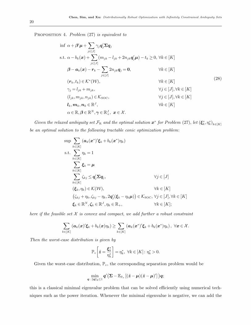
Proposition 4. Problem (27) is equivalent to
inf α+β′µ+∑j∈[J]
γjq′jΣqj
s.t. α− bk(x) +∑j∈[J]
(mjk− ljk + 2njkq′jµ)− tk ≥ 0, ∀k ∈ [K]
β−ak(x)− rk−∑j∈[J]
2njkqj = 0, ∀k ∈ [K]
(rk, tk)∈K∗(W), ∀k ∈ [K]
γj = ljk +mjk, ∀j ∈ [J ],∀k ∈ [K]
(ljk,mjk, njk)∈KSOC, ∀j ∈ [J ],∀k ∈ [K]
lk,mk,nk ∈RJ , ∀k ∈ [K]
α∈R,β ∈RN ,γ ∈RJ+, x∈X .
(28)
Given the relaxed ambiguity set FR and the optimal solution x∗ for Problem (27), let (ξ∗k, η∗k)k∈[K]
be an optimal solution to the following tractable conic optimization problem:
sup∑k∈[K]
(ak(x∗)′ξk + bk(x
∗)ηk)
s.t.∑k∈[K]
ηk = 1∑k∈[K]
ξk =µ∑k∈[K]
ζkj ≤ q′jΣqj, ∀j ∈ [J ]
(ξk, ηk)∈K(W), ∀k ∈ [K](ζkj + ηk, ζkj − ηk,2q′j(ξk− ηkµ)
)∈KSOC, ∀j ∈ [J ],∀k ∈ [K]
ξk ∈RN ,ζk ∈RJ , ηk ∈R+, ∀k ∈ [K];
here if the feasible set X is convex and compact, we add further a robust constraint∑k∈[K]
(ak(x)′ξk + bk(x)ηk)≥∑k∈[K]
(ak(x∗)′ξk + bk(x
∗)ηk) , ∀x∈X .
Then the worst-case distribution is given by
Pv[z =
ξ∗kη∗k
]= η∗k, ∀k ∈ [K] : η∗k > 0.
Given the worst-case distribution, Pv, the corresponding separation problem would be
minq : ‖q‖2≤1
q′(Σ−EPv [(z−µ)(z−µ)′]
)q;
this is a classical minimal eigenvalue problem that can be solved efficiently using numerical tech-
niques such as the power iteration. Whenever the minimal eigenvalue is negative, we can add the

Chen, Sim, and Xu: Distributionally Robust Optimization with Infinitely Constrained Ambiguity Sets
21
corresponding eigenvector to the set Q, which would end up tightening the relaxed covariance
ambiguity set GC. It is of considerable interest that there exists an ambiguity set GC with J =N
such that Problems (24) and (27) have the same objective value, as shown in the following result.
Theorem 6. Consider any function f : RN 7→R, for which the problem
supP∈FC
EP [f(z)]
is finitely optimal. There exists a relaxed ambiguity set G∗C such that J =N and
supP∈FC
EP [f(z)] = supP∈G∗
C
EP [f(z)] .
Proof. Consider the problem ZA = supP∈FC EP [f(z)]. By duality, we have
ZA = inf α+β′µ+ 〈Γ,Σ〉
s.t. α+β′z+⟨Γ, (z−µ)(z−µ)′
⟩≥ f(z), ∀z ∈W
α∈R,β ∈RN ,Γ� 0,
(29)
whose optimal solution we denote by (α∗,β∗,Γ∗). Using the eigendecomposition, we write Γ∗ =∑n∈[N ] λ
∗nq∗n(q∗n)′, where the {λ∗n}n∈[N ] are eigenvalues of Γ∗ and where {q∗n}n∈[N ] are the corre-
sponding eigenvectors. Note that Γ∗ � 0 implies that λ∗n ≥ 0 for all n∈ [N ].
Let G∗C be the particular relaxed ambiguity set with Q= {q∗1 , . . . ,q∗N} and consider the problem
ZB = supP∈G∗CEP [f(z)], whose dual is given as follows:
ZB = inf α+β′µ+∑n∈[N ]
γn(q∗n)′Σq∗n
s.t. α+β′z+∑n∈[N ]
γn((q∗n)′(z−µ))2 ≥ f(z), ∀z ∈W
α∈R,β ∈RN ,γ ∈RN+ .
(30)
We can exploit the optimal solution to Problem (29) to construct a feasible solution (αB,βB,γB)
to Problem (30) by letting αB = α∗, βB =β∗, and γB =λ∗. Since 〈Γ∗,Σ〉=∑
n∈[N ] 〈λ∗nq∗n(q∗n)′,Σ〉=∑n∈[N ] γn(q∗n)′Σq∗n, it follows that ZB ≤ ZA. Yet we already know that ZA ≤ ZB for any relaxed
covariance ambiguity set, so our claim holds. �
Having a relaxation of Problem (24) in the form of a second-order conic program is especially
useful when the feasible set X has integral constraints because such a format is already supported
by commercial solvers such as CPLEX and Gurobi. In such cases, the reformulation of Problem (24)
would become a semidefinite program involving discrete decision variables, which are harder to
solve. Instead, we can first consider the linear relaxation of X (denoted by X ), solve the problem
minx∈X
supP∈FC
EP [f(x, z)] ,

Chen, Sim, and Xu: Distributionally Robust Optimization with Infinitely Constrained Ambiguity Sets
22
and obtain G∗C through Theorem 6. Afterward, we implement Algorithm GIP with G∗C being the
initial relaxed ambiguity set and solve a sequence of mixed-integer second-order conic programs to
obtain approximate solutions to the problem of interest.
Fourth moment ambiguity set
The fourth moment ambiguity set (8) has the following relaxation
GF =
P∈P0
(RN)∣∣∣∣∣∣∣∣∣∣∣∣∣∣
z ∼ P
EP [z] = 0
EP [(q′z)2]≤ q′Σq, ∀q ∈ Q
EP [(q′z)4]≤ϕ(q), ∀q ∈ Q
P [z ∈W] = 1
, (31)
where Q= {qj | j ∈ [J ]} and Q= {qj | j ∈ [J ]} for some qj,qj ∈RN and ‖qj‖2,‖qj‖2 ≤ 1. Note that
the function (q′z)4 is also second-order conic representable in z. Following from a similar derivation
as in Proposition 4, the relaxed distributionally robust optimization problem
minx∈X
supP∈GF
EP [f(x, z)]
can be reformulated as a second-order conic program and so does the optimization problem for
determining the worst-case distribution. Given that the worst-case distribution Pv takes value zk
with probability pk, the separation problem that corresponds to the second set of infinitely many
expectation constraints in FF is unconstrained and takes the following form:
minq
Ψ(q) = minq
{ ∑n∈[N ]
(q4nκ
4n + 6
∑m 6=n
q2mq
2nσ
2mσ
2n
)−∑k∈[K]
pk(q′zk)
4
},
where the objective function is a multivariate polynomial of {q}n∈[N ]. In general, this separation
problem is NP-hard (Nesterov 2000) but admits a semidefinite relaxation if we use the sum of
squares tool (cf. Choi et al. 1995, Lasserre 2001, Parrilo 2003). This kind of semidefinite relaxations
may be successively improved and has been applied in many areas including option pricing (Bert-
simas and Popescu 2002, Lasserre et al. 2006). An alternative approach is to adopt the trust region
method (TRM), which is useful for finding local minimums of this separation problem. The TRM
is one of the most important numerical optimization methods in solving nonlinear programming
problems. It works by solving a sequence of subproblems; in each subproblem, the TRM approxi-
mates the objective function Ψ(·) by a quadratic function (usually obtained by taking Taylor series
up to second order) and searches for an improving direction in a region around the current solution.
Note that solving an unconstrained nonlinear optimization problem via the TRM is well supported
in Matlab (Mathworks 2017); we need only provide the gradient and the Hessian matrix of Ψ(·).
Chen, Sim, and Xu: Distributionally Robust Optimization with Infinitely Constrained Ambiguity Sets
23
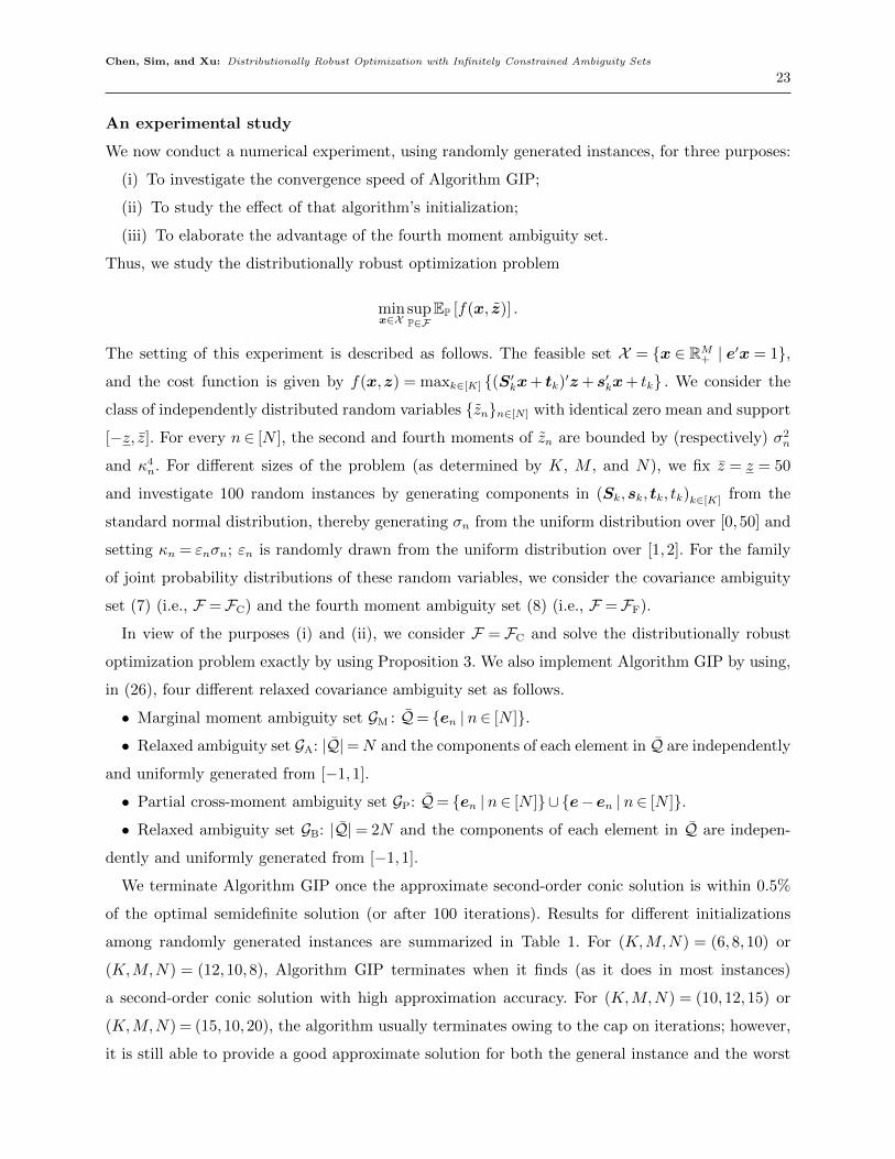
An experimental study
We now conduct a numerical experiment, using randomly generated instances, for three purposes:
(i) To investigate the convergence speed of Algorithm GIP;
(ii) To study the effect of that algorithm’s initialization;
(iii) To elaborate the advantage of the fourth moment ambiguity set.
Thus, we study the distributionally robust optimization problem
minx∈X
supP∈F
EP [f(x, z)] .
The setting of this experiment is described as follows. The feasible set X = {x ∈ RM+ | e′x = 1},
and the cost function is given by f(x,z) = maxk∈[K] {(S′kx+ tk)′z+ s′kx+ tk} . We consider the
class of independently distributed random variables {zn}n∈[N ] with identical zero mean and support
[−z, z]. For every n∈ [N ], the second and fourth moments of zn are bounded by (respectively) σ2n
and κ4n. For different sizes of the problem (as determined by K, M , and N), we fix z = z = 50
and investigate 100 random instances by generating components in (Sk,sk, tk, tk)k∈[K] from the
standard normal distribution, thereby generating σn from the uniform distribution over [0,50] and
setting κn = εnσn; εn is randomly drawn from the uniform distribution over [1,2]. For the family
of joint probability distributions of these random variables, we consider the covariance ambiguity
set (7) (i.e., F =FC) and the fourth moment ambiguity set (8) (i.e., F =FF).
In view of the purposes (i) and (ii), we consider F = FC and solve the distributionally robust
optimization problem exactly by using Proposition 3. We also implement Algorithm GIP by using,
in (26), four different relaxed covariance ambiguity set as follows.
• Marginal moment ambiguity set GM : Q= {en | n∈ [N ]}.
• Relaxed ambiguity set GA: |Q|=N and the components of each element in Q are independently
and uniformly generated from [−1,1].
• Partial cross-moment ambiguity set GP: Q= {en | n∈ [N ]}∪ {e−en | n∈ [N ]}.
• Relaxed ambiguity set GB: |Q|= 2N and the components of each element in Q are indepen-
dently and uniformly generated from [−1,1].
We terminate Algorithm GIP once the approximate second-order conic solution is within 0.5%
of the optimal semidefinite solution (or after 100 iterations). Results for different initializations
among randomly generated instances are summarized in Table 1. For (K,M,N) = (6,8,10) or
(K,M,N) = (12,10,8), Algorithm GIP terminates when it finds (as it does in most instances)
a second-order conic solution with high approximation accuracy. For (K,M,N) = (10,12,15) or
(K,M,N) = (15,10,20), the algorithm usually terminates owing to the cap on iterations; however,
it is still able to provide a good approximate solution for both the general instance and the worst
Chen, Sim, and Xu: Distributionally Robust Optimization with Infinitely Constrained Ambiguity Sets
24
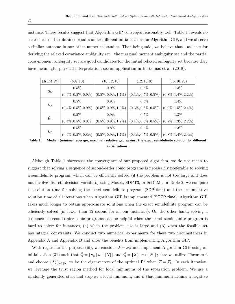
instance. These results suggest that Algorithm GIP converges reasonably well. Table 1 reveals no
clear effect on the obtained results under different initializations for Algorithm GIP, and we observe
a similar outcome in our other numerical studies. That being said, we believe that—at least for
deriving the relaxed covariance ambiguity set—the marginal moment ambiguity set and the partial
cross-moment ambiguity set are good candidates for the initial relaxed ambiguity set because they
have meaningful physical interpretation; see an application in Bertsimas et al. (2018).
(K,M,N) (6,8,10) (10,12,15) (12,10,8) (15,10,20)
GM0.5%
(0.4%,0.5%,0.9%)
0.9%
(0.5%,0.9%,1.7%)
0.5%
(0.3%,0.5%,0.5%)
1.3%
(0.8%,1.4%,2.2%)
GA0.5%
(0.4%,0.5%,0.9%)
0.9%
(0.5%,0.9%,1.9%)
0.5%
(0.3%,0.5%,0.5%)
1.4%
(0.9%,1.5%,2.4%)
GP0.5%
(0.4%,0.5%,0.8%)
0.9%
(0.5%,0.9%,1.7%)
0.5%
(0.4%,0.5%,0.5%)
1.3%
(0.7%,1.3%,2.2%)
GB0.5%
(0.4%,0.5%,0.8%)
0.8%
(0.5%,0.9%,1.7%)
0.5%
(0.3%,0.5%,0.5%)
1.3%
(0.8%,1.4%,2.3%)
Table 1 Median (minimal, average, maximal) relative gap against the exact semidefinite solution for different
initializations.
Although Table 1 showcases the convergence of our proposed algorithm, we do not mean to
suggest that solving a sequence of second-order conic programs is necessarily preferable to solving
a semidefinite program, which can be efficiently solved (if the problem is not too large and does
not involve discrete decision variables) using Mosek, SDPT3, or SeDuMi. In Table 2, we compare
the solution time for solving the exact semidefinite program (SDP time) and the accumulative
solution time of all iterations when Algorithm GIP is implemented (SOCP time). Algorithm GIP
takes much longer to obtain approximate solutions when the exact semidefinite program can be
efficiently solved (in fewer than 12 second for all our instances). On the other hand, solving a
sequence of second-order conic programs can be helpful when the exact semidefinite program is
hard to solve: for instances, (a) when the problem size is large and (b) when the feasible set
has integral constraints. We conduct two numerical experiments for these two circumstances in
Appendix A and Appendix B and show the benefits from implementing Algorithm GIP.
With regard to the purpose (iii), we consider F = FF and implement Algorithm GIP using an
initialization (31) such that Q= {en | n ∈ [N ]} and Q= {λ∗n | n ∈ [N ]}; here we utilize Theorem 6
and choose {λ∗n}n∈[N ] to be the eigenvectors of the optimal Γ∗ when F = FC. In each iteration,
we leverage the trust region method for local minimums of the separation problem. We use a
randomly generated start and stop at a local minimum, and if that minimum attains a negative

Chen, Sim, and Xu: Distributionally Robust Optimization with Infinitely Constrained Ambiguity Sets
25
(K,M,N) (6,8,10) (10,12,15) (12,10,8) (15,10,20)
GM 4.5 4.5 0.7 4.5
GA 5.0 4.6 1.1 4.9
GP 5.5 6.1 0.9 7.0
GB 5.4 5.8 1.2 6.7
Table 2 Average SOCP time/SDP time for different initializations.
objective value for the separation problem then we find a violating expectation constraint and
proceed to the next iteration; otherwise, we continue with another random start. We terminate
Algorithm GIP if no violating expectation constraint is found after 100 trials for a given iteration
(or after 50 iterations). The relative improvement from considering the fourth moment ambiguity
set is reported in Table 3, which shows the clear improvement for all four problem sizes. We
remark that this improvement accounts only for the best approximation we have sought—because
finding the separation problem’s optimal solution is hard and we have to terminate Algorithm GIP
prematurely.
(K,M,N) (6,8,10) (10,12,15) (12,10,8) (15,10,20)
Relative
improvement
1.8%
(0.3%,1.9%,5.1%)
3.9%
(1.4%,4.2%,7.5%)
4.5%
(1.6%,4.6%,9.9%)
5.1%
(2.0%,5.2%,7.2%)
Table 3 Median (minimal, average, maximal) relative improvement over the semidefinite solution.
5. Entropic dominance
In this section, we focus on the entropic dominance ambiguity set FE in (9) and show that it
provides a better characterization of stochastic independence than does the covariance ambiguity
set. In particular, we consider the relaxed distributionally robust optimization problem
minx∈X
supP∈GE
EP [f(x, z)] (32)
with the relaxed entropic dominance ambiguity set
GE =
P∈P0
(RN)∣∣∣∣∣∣∣∣∣∣∣
z ∼ P
EP [z] =µ
lnEP [exp (q′(z−µ))]≤ φ(q), ∀q ∈ Q
P [z ∈W] = 1
,
where Q = {qj | j ∈ [J ]} for some qj ∈ RN . As mentioned in Section 2, we explicitly specify the
mean and support because they are not implied when there are only a finite number of expectation

Chen, Sim, and Xu: Distributionally Robust Optimization with Infinitely Constrained Ambiguity Sets
26
constraints in GE. Problem (32) can be reformulated as a conic optimization problem involving the
exponential cone, as can the problem for obtaining the worst-case distribution.
Proposition 5. Problem (32) is equivalent to
inf α+β′µ+∑j∈[j]
γj
s.t. α− bk(x) +∑j∈[J]
lkj(q′jµ+φ (qj)
)−∑j∈[J]
mkj − tk ≥ 0, ∀k ∈ [K]
β−ak(x)− rk−∑j∈[J]
lkjqj = 0, ∀k ∈ [K]
γ−nk = 0, ∀k ∈ [K]
(lkj,mkj, nkj)∈K∗EXP, ∀j ∈ [J ],∀k ∈ [K]
(rk, tk)∈K∗(W), ∀k ∈ [K]
α∈R,β ∈RN ,γ ∈RJ+, x∈X .
Given the relaxed ambiguity set FR and the optimal solution x∗ for Problem (32), let (ξ∗k, η∗k)k∈[K]
be an optimal solution to the following tractable conic optimization problem:
sup∑k∈[K]
(ak(x∗)′ξk + bk(x
∗)ηk)
s.t.∑k∈[K]
ηk = 1∑k∈[K]
ξk =µ∑k∈[K]
ζk ≤ e
(ξk, ηk)∈K(W), ∀k ∈ [K](q′j(ξk− ηkµ)− ηkφ(qj), ηk, ζkj
)∈KEXP, ∀j ∈ [J ], k ∈ [K]
ξk ∈RN ,ζk ∈RJ , ηk ∈R+, ∀k ∈ [K];
here if the feasible set X is convex and compact, we add further a robust constraint∑k∈[K]
(ak(x)′ξk + bk(x)ηk)≥∑k∈[K]
(ak(x∗)′ξk + bk(x
∗)ηk) , ∀x∈X .
Then the worst-case distribution is given by
Pv[z =
ξ∗kη∗k
]= η∗k, ∀k ∈ [K] : η∗k > 0.
Note that an exponential conic constraint can be approximated fairly accurately via a small
number of second-order conic constraints (see Chen and Sim 2009, Appendix B). This kind of
successive approximation methods is supported in Matlab toolboxes, such as ROME (Goh and
Sim 2011) and CVX (Grant and Boyd 2008, Grant et al. 2008). An exponential conic program

Chen, Sim, and Xu: Distributionally Robust Optimization with Infinitely Constrained Ambiguity Sets
27
can also be efficiently and exactly solved by interior-point methods (cf. Chares 2009, Skajaa and
Ye 2015). For the entropic dominance ambiguity set, the corresponding separation problem is
unconstrained and takes the following form:
minq
Φ(q) = minq{φ(q)− lnEPv [exp(q′(z−µ))]}= min
q
{φ(q)− ln
∑k∈[K]
pk exp(q′(zk−µ)
)};
here the worst-case distribution Pv takes value zk with probability pk. We can also use the TRM
for efficiently detection of the local minimums.
An application in portfolio selection
In this numerical example, we illustrate how our new bound for the expected surplus EP [(·)+]
can be leveraged in practice. For that purpose, we study the distributionally robust portfolio
optimization problem under the worst-case conditional value at risk (CVaR) of Rockafellar and
Uryasev (2002). We consider the case of N assets, each with independently distributed random
return premium µn+σnzn that are affected by the uncertainty zn with mean 0 and support [−1,1].
The parameters used in our study are N = 50, µn = n/250, and σn = (N√
2n)/1000. Thus, the asset
with a higher return premium is more risky. The feasible investment lies in the simplex x ∈ X =
{x∈RN+ | e′x= 1}. The total return premium obtained from an investment x under realization z is
L(x,z) =∑
n∈[N ] xn(µn +σnzn). Inspired by Zymler et al. (2013), we consider the distributionally
robust optimization model, which looks for an investment plan with minimal worst-case CVaR:
minx∈X
supP∈F
P-CVaRε (−L(x, z)) , (33)
where the CVaR at level ε with respect to a probability distribution P is
P-CVaRε (−L(x,x)) = minθ∈R
{θ+
1
εEP[(−L(x, z)− θ)+ ]}
.
By the stochastic minimax theorem in Shapiro and Kleywegt (2002), we can rewrite the worst-case
CVaR in the objective function of Problem (33) as
supP∈F
P-CVaRε (−L(x,x)) = minθ∈R
{θ+
1
εsupP∈F
EP[(−L(x, z)− θ)+ ]}
.
As a result, the worst-case CVaR portfolio selection problem (33) becomes
minx∈X ,θ∈R
{θ+
1
εsupP∈F
EP[(−L(x, z)− θ)+ ]}
.
We consider the following covariance ambiguity set, which encompasses the family of distributions
of these independently distributed uncertainties {zn}n∈[N ]:
FC =
P∈P0
(RN)∣∣∣∣∣∣∣∣∣∣∣
z ∼ P
EP [z] = 0
EP
[(q′z)
2]≤ q′q, ∀q ∈RN : ‖q‖2 ≤ 1
P [z ∈W] = 1
,

Chen, Sim, and Xu: Distributionally Robust Optimization with Infinitely Constrained Ambiguity Sets
28
where the support set is modeled asW = {z ∈RN | ‖z‖∞ ≤ 1}. Because zn is sub-Gaussian with zero
mean and unit deviation parameter for n∈ [N ], we also consider the following entropic ambiguity
set (which captures the sub-Gaussianity):
FG =
P∈P0
(RN)∣∣∣∣∣∣∣∣∣∣∣∣
z ∼ P
EP [z] = 0
lnEP [exp (q′z)]≤ 1
2q′q, ∀q ∈RN
P [z ∈W] = 1
;
here we explicitly specify the support set W because, by Theorem 2, the chosen function φ(·)
implies only thatW lies in RN . As shown in the following result, the entropic dominance ambiguity
set improves upon the covariance ambiguity set in terms of capturing independently distributed
random variables with known mean and support.
Proposition 6. Let z1, . . . , zN be independently distributed random variables of zero mean and
with support W = {z ∈ RN | ‖z‖∞ ≤ 1}. The minimal covariance ambiguity set that encompasses
this family of distributions is FC. The entropic dominance ambiguity set FG yields a better char-
acterization of this family of distributions: that is, FG ⊆FC.
We now investigate the numerical performance of the relaxed entropic dominance ambiguity set
GG =
P∈P0
(RN)∣∣∣∣∣∣∣∣∣∣∣∣
z ∼ P
EP [z] = 0
lnEP [exp (q′z)]≤ 1
2q′q, ∀q ∈ Q
P [z ∈W] = 1
against the covariance ambiguity set FC. We initialize Algorithm GIP with Q = {en | n ∈ [N ]}.
In each iteration, we solve the separation problem by the trust region method with a randomly
generated initial solution. If the resulting local minimum attains a negative objective value, then
we find a violating expectation constraint and proceed to the next iteration; otherwise, we continue
with the TRM while using another randomly generated initial solution. The algorithm terminates
if no violating expectation constraint is found after 100 trials.
We report the objective values for various confidence levels, ε ∈ {0.01,0.02,0.05,0.08,0.1}, in
Table 4. Note that ZC denotes the objective value obtained by the covariance ambiguity set and that
ZiG denotes the objective value achieved at the i-th iteration when using the entropic dominance
ambiguity set. The relaxed entropic dominance solutions yield significantly lower objective values
than those obtained from the covariance ambiguity set. Moreover, the entropic dominance approach
converges reasonably well: it terminates in at most 10 iterations. As a robustness check, we used

Chen, Sim, and Xu: Distributionally Robust Optimization with Infinitely Constrained Ambiguity Sets
29
different initializations for the relaxed entropic dominance ambiguity set; we arrived at the same
solutions and observed similar convergence results.
ε 0.01 0.02 0.05 0.08 0.1
ZC 0.0674 0.0674 0.0674 0.0579 0.0430
Z1G 0.0674 0.0674 0.0674 0.0674 0.0674
Z2G 0.0674 0.0674 0.0674 0.0661 0.0661
Z3G 0.0474 0.0674 0.0484 0.0251 0.0569
Z4G 0.0443 0.0408 0.0247 0.0126 0.0517
Z5G 0.0442 0.0350 0.0201 0.0126 0.0486
Z6G — 0.0347 0.0199 0.0106 0.0163
Z7G — — 0.0199 0.0105 0.0069
Z8G — — — 0.0105 0.0055
Z9G — — — — 0.0054
Z10G — — — — —
Table 4 Objective values of the covariance approach and the entropic dominance approach.
6. Future work
In this paper, we work with static distributionally robust optimization problems. In our numerical
studies, we choose the marginal moment ambiguity set and the partial cross-moment ambiguity
set as the relaxed covariance ambiguity set and identify “violating” expectation constraints to
improve the solution. In a recent work, Bertsimas et al. (2018) study adaptive distributionally
robust optimization problems and show the improvement of the partial cross-moment ambiguity
set over the marginal moment ambiguity set. We believe that the extension of our approach to
adaptive problems with infinitely constrained ambiguity sets and to systematically improve the
partial cross-moment ambiguity set (or any relaxed ambiguity set) will be useful.
Acknowledgments
The authors would like to thank Daniel Kuhn and Wolfram Wiesemann for the helpful discussions and
comments. The authors also thank Zhenyu Hu and Karthik Natarajan for their feedbacks. The research of
Melvyn Sim is supported by the Singapore National Research Foundation National Cybersecurity R&D Grant
under Grant R-263-000-C74-281 and Grant NRF2015NCR-NCR003-006. The research of Huan Xu is partly
supported by the startup fund from the H. Milton Stewart School of Industrial and Systems Engineering of
Georgia Institute of Technology.

Chen, Sim, and Xu: Distributionally Robust Optimization with Infinitely Constrained Ambiguity Sets
30
References
Ben-Tal, Aharon, Dick Den Hertog, Anja De Waegenaere, Bertrand Melenberg, Gijs Rennen. 2013. Robust
solutions of optimization problems affected by uncertain probabilities. Management Science 59(2)
341–357.
Ben-Tal, Aharon, Arkadi Nemirovski. 1998. Robust convex optimization. Mathematics of operations research
23(4) 769–805.
Ben-Tal, Aharon, Arkadi Nemirovski. 2001. Lectures on modern convex optimization: analysis, algorithms,
and engineering applications. SIAM.
Bertsimas, Dimitris, Ioana Popescu. 2002. On the relation between option and stock prices: a convex opti-
mization approach. Operations Research 50(2) 358–374.
Bertsimas, Dimitris, Ioana Popescu. 2005. Optimal inequalities in probability theory: A convex optimization
approach. SIAM Journal on Optimization 15(3) 780–804.
Bertsimas, Dimitris, Melvyn Sim. 2004. The price of robustness. Operations research 52(1) 35–53.
Bertsimas, Dimitris, Melvyn Sim, Meilin Zhang. 2018. Adaptive distributionally robust optimization. Man-
agement Science .
Birge, John R, Francois Louveaux. 2011. Introduction to stochastic programming . Springer Science & Business
Media.
Breton, Michele, Saeb El Hachem. 1995. Algorithms for the solution of stochastic dynamic minimax problems.
Computational Optimization and Applications 4(4) 317–345.
Chares, Robert. 2009. Cones and interior-point algorithms for structured convex optimization involving
powers and exponentials. PhD thesis .
Chen, Wenqing, Melvyn Sim. 2009. Goal-driven optimization. Operations Research 57(2) 342–357.
Chen, Wenqing, Melvyn Sim, Jie Sun, Chung-Piaw Teo. 2010. From cvar to uncertainty set: Implications in
joint chance-constrained optimization. Operations research 58(2) 470–485.
Chen, Xin, Melvyn Sim, Peng Sun. 2007. A robust optimization perspective on stochastic programming.
Operations Research 55(6) 1058–1071.
Chen, Xin, Melvyn Sim, Peng Sun, Jiawei Zhang. 2008. A linear decision-based approximation approach to
stochastic programming. Operations Research 56(2) 344–357.
Chen, Zhi, Melvyn Sim, Peng Xiong. 2017. Tractable distributionally robust optimization with data. URL
http://www.optimization-online.org/DB_FILE/2017/06/6055.pdf.
Choi, Man-Duen, Tsit Yuen Lam, Bruce Reznick. 1995. Sums of squares of real polynomials. Proceedings of
Symposia in Pure mathematics, vol. 58. American Mathematical Society, 103–126.
Conn, Andrew R, Nicholas IM Gould, Philippe L Toint. 2000. Trust region methods. SIAM.
Chen, Sim, and Xu: Distributionally Robust Optimization with Infinitely Constrained Ambiguity Sets
31
Delage, Erick, Yinyu Ye. 2010. Distributionally robust optimization under moment uncertainty with appli-
cation to data-driven problems. Operations research 58(3) 595–612.
Dentcheva, Darinka, Andrzej Ruszczynski. 2003. Optimization with stochastic dominance constraints. SIAM
Journal on Optimization 14(2) 548–566.
Dentcheva, Darinka, Andrzej Ruszczynski. 2006. Portfolio optimization with stochastic dominance con-
straints. Journal of Banking & Finance 30(2) 433–451.
Dupacova, Jitka. 1987. The minimax approach to stochastic programming and an illustrative application.
Stochastics: An International Journal of Probability and Stochastic Processes 20(1) 73–88.
El Ghaoui, Laurent, Maksim Oks, Francois Oustry. 2003. Worst-case value-at-risk and robust portfolio
optimization: A conic programming approach. Operations research 51(4) 543–556.
El Ghaoui, Laurent, Francois Oustry, Herve Lebret. 1998. Robust solutions to uncertain semidefinite pro-
grams. SIAM Journal on Optimization 9(1) 33–52.
Esfahani, Peyman Mohajerin, Daniel Kuhn. 2017. Data-driven distributionally robust optimization using the
wasserstein metric: Performance guarantees and tractable reformulations. Mathematical Programming
1–52.
Gao, Rui, Anton J Kleywegt. 2016. Distributionally robust stochastic optimization with wasserstein distance.
arXiv preprint arXiv:1604.02199 .
Gilboa, Itzhak, David Schmeidler. 1989. Maxmin expected utility with non-unique prior. Journal of mathe-
matical economics 18(2) 141–153.
Goh, Joel, Melvyn Sim. 2010. Distributionally robust optimization and its tractable approximations. Oper-
ations research 58(4-part-1) 902–917.
Goh, Joel, Melvyn Sim. 2011. Robust optimization made easy with rome. Operations Research 59(4)
973–985.
Grant, Michael, Stephen Boyd, Yinyu Ye. 2008. Cvx: Matlab software for disciplined convex programming.
Grant, Michael C, Stephen P Boyd. 2008. Graph implementations for nonsmooth convex programs. Recent
advances in learning and control . Springer, 95–110.
Hanasusanto, Grani A, Daniel Kuhn, Wolfram Wiesemann. 2016. A comment on computational complexity
of stochastic programming problems. Mathematical Programming 159(1-2) 557–569.
Hanasusanto, Grani A, Vladimir Roitch, Daniel Kuhn, Wolfram Wiesemann. 2017. Ambiguous joint chance
constraints under mean and dispersion information. Operations Research 65(3) 751–767.
He, Simai, Jiawei Zhang, Shuzhong Zhang. 2010. Bounding probability of small deviation: A fourth moment
approach. Mathematics of Operations Research 35(1) 208–232.
Isii, Keiiti. 1962. On sharpness of tchebycheff-type inequalities. Annals of the Institute of Statistical Mathe-
matics 14(1) 185–197.

Chen, Sim, and Xu: Distributionally Robust Optimization with Infinitely Constrained Ambiguity Sets
32
Jiang, Ruiwei, Yongpei Guan. 2016. Data-driven chance constrained stochastic program. Mathematical
Programming 158(1-2) 291–327.
Kaas, Rob, Marc Goovaerts, Jan Dhaene, Michel Denuit. 2008. Modern actuarial risk theory: using R, vol.
128. Springer Science & Business Media.
Lasserre, Jean B. 2001. Global optimization with polynomials and the problem of moments. SIAM Journal
on Optimization 11(3) 796–817.
Lasserre, Jean-Bernard, Tomas Prieto-Rumeau, Mihail Zervos. 2006. Pricing a class of exotic options via
moments and sdp relaxations. Mathematical Finance 16(3) 469–494.
Mathworks. 2017. Unconstrained nonlinear optimization algorithms. URL www.mathworks.com/help/
optim/ug/unconstrained-nonlinear-optimization-algorithms.html.
Nemirovski, Arkadi, Alexander Shapiro. 2006. Convex approximations of chance constrained programs.
SIAM Journal on Optimization 17(4) 969–996.
Nesterov, Yurii. 2000. Squared functional systems and optimization problems. High performance optimiza-
tion. Springer, 405–440.
Parrilo, Pablo A. 2003. Semidefinite programming relaxations for semialgebraic problems. Mathematical
programming 96(2) 293–320.
Pflug, Georg, David Wozabal. 2007. Ambiguity in portfolio selection. Quantitative Finance 7(4) 435–442.
Postek, Krzysztof, Aharon Ben-Tal, Dick den Hertog, Bertrand Melenberg. 2018. Robust optimization with
ambiguous stochastic constraints under mean and dispersion information. Operations Research .
Rockafellar, R Tyrrell, Stanislav Uryasev. 2002. Conditional value-at-risk for general loss distributions.
Journal of banking & finance 26(7) 1443–1471.
Scarf, Herbert. 1958. A min-max solution of an inventory problem. Studies in the mathematical theory of
inventory and production .
Shapiro, Alexander. 2001. On duality theory of conic linear problems. Semi-infinite programming . Springer,
135–165.
Shapiro, Alexander, Anton Kleywegt. 2002. Minimax analysis of stochastic problems. Optimization Methods
and Software 17(3) 523–542.
Sion, Maurice. 1958. On general minimax theorems. Pacific Journal of mathematics 8(1) 171–176.
Skajaa, Anders, Yinyu Ye. 2015. A homogeneous interior-point algorithm for nonsymmetric convex conic
optimization. Mathematical Programming 150(2) 391–422.
Soyster, Allen L. 1973. Technical noteconvex programming with set-inclusive constraints and applications
to inexact linear programming. Operations research 21(5) 1154–1157.
von Neumann, John, Oskar Morgenstern. 1947. Theory of games and economic behavior . Princeton university
press.

Chen, Sim, and Xu: Distributionally Robust Optimization with Infinitely Constrained Ambiguity Sets
33
Wainwright, JM. 2015. High-dimensional statistics: A non-asymptotic viewpoint . Preparation. University of
California, Berkeley.
Wang, Zizhuo, Peter W Glynn, Yinyu Ye. 2016. Likelihood robust optimization for data-driven problems.
Computational Management Science 13(2) 241–261.
Wiesemann, Wolfram, Daniel Kuhn, Melvyn Sim. 2014. Distributionally robust convex optimization. Oper-
ations Research 62(6) 1358–1376.
Zhao, Chaoyue, Yongpei Guan. 2018. Data-driven risk-averse stochastic optimization with wasserstein metric.
Operations Research Letters 46(2) 262–267.
Zymler, Steve, Daniel Kuhn, Berc Rustem. 2013. Distributionally robust joint chance constraints with
second-order moment information. Mathematical Programming 1–32.

e-companion to Chen, Sim, and Xu: Distributionally Robust Optimization with Infinitely Constrained Ambiguity Sets ec1
Eletronic Companion
Appendix A
We conduct an experiment using randomly generated instances of the following distributionally
robust optimization problem
minx∈X
supP∈FC
EP [f(x, z)] ,
where FC is a covariance ambiguity set. The setting of this experiment is identical to that in the
paper. We increase the size of the problem (as determined by K, M , and N) so that the computer
can not solve the exact semidefinite reformulation within an hour. We implement Algorithm GIP
by using the partial cross-moment ambiguity set with Q= {en | n∈ [N ]}∪{e} as the initial relaxed
ambiguity set. We terminate Algorithm GIP after 50 iterations (the accumulative solution time of
all iterations is less than an hour).
Let ZiC denote the objective value achieved at the i-th iteration when using the relaxed ambiguity
set. We report in Table EC.1 the relative gap (over 10 random instances for each size of the
problem) between the initial solution Z1C and the terminal solution Z50
C , which is given by∣∣∣∣Z1C−Z50
C
Z50C
∣∣∣∣× 100%.
The result reveals that by solving a sequence of second-order conic subproblems, Algorithm GIP
yields iteratively an improved solution, even when the exact semidefinite program can not be solved
within the time limit. This experiment supports that having a second-order conic relaxation can
be helpful when the exact semidefinite program is of a large size.
(K,M,N) (110,20,50) (100,20,60) (80,20,70)
Relative
improvement
12.0%
(10.5%,12.1%,13.9%)
12.8%
(10.9%,12.9%,14.4%)
14.3%
(13.3%,14.4%,16.2%)
Table EC.1 Median (minimal, average, maximal) relative gap.
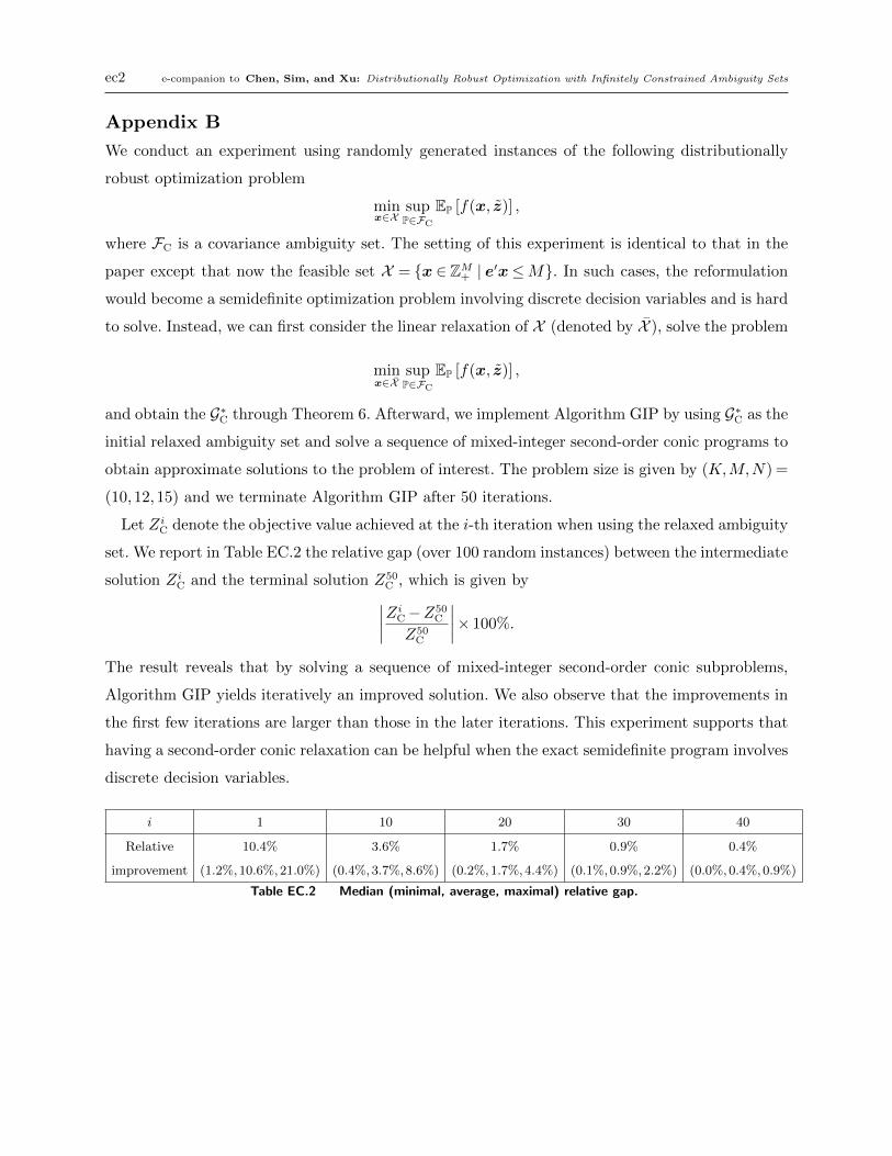
ec2 e-companion to Chen, Sim, and Xu: Distributionally Robust Optimization with Infinitely Constrained Ambiguity Sets
Appendix B
We conduct an experiment using randomly generated instances of the following distributionally
robust optimization problem
minx∈X
supP∈FC
EP [f(x, z)] ,
where FC is a covariance ambiguity set. The setting of this experiment is identical to that in the
paper except that now the feasible set X = {x ∈ ZM+ | e′x≤M}. In such cases, the reformulation
would become a semidefinite optimization problem involving discrete decision variables and is hard
to solve. Instead, we can first consider the linear relaxation of X (denoted by X ), solve the problem
minx∈X
supP∈FC
EP [f(x, z)] ,
and obtain the G∗C through Theorem 6. Afterward, we implement Algorithm GIP by using G∗C as the
initial relaxed ambiguity set and solve a sequence of mixed-integer second-order conic programs to
obtain approximate solutions to the problem of interest. The problem size is given by (K,M,N) =
(10,12,15) and we terminate Algorithm GIP after 50 iterations.
Let ZiC denote the objective value achieved at the i-th iteration when using the relaxed ambiguity
set. We report in Table EC.2 the relative gap (over 100 random instances) between the intermediate
solution ZiC and the terminal solution Z50C , which is given by∣∣∣∣ZiC−Z50
C
Z50C
∣∣∣∣× 100%.
The result reveals that by solving a sequence of mixed-integer second-order conic subproblems,
Algorithm GIP yields iteratively an improved solution. We also observe that the improvements in
the first few iterations are larger than those in the later iterations. This experiment supports that
having a second-order conic relaxation can be helpful when the exact semidefinite program involves
discrete decision variables.
i 1 10 20 30 40
Relative
improvement
10.4%
(1.2%,10.6%,21.0%)
3.6%
(0.4%,3.7%,8.6%)
1.7%
(0.2%,1.7%,4.4%)
0.9%
(0.1%,0.9%,2.2%)
0.4%
(0.0%,0.4%,0.9%)
Table EC.2 Median (minimal, average, maximal) relative gap.

e-companion to Chen, Sim, and Xu: Distributionally Robust Optimization with Infinitely Constrained Ambiguity Sets ec3
Appendix C
Proof of Theorem 2. Consider any probability distribution P∈FE and observe that
EP [zn−µn] = limα→0
EP [exp (α(zn−µn))]− 1
α.
Let α→ 0+(0−); then
limα→0+(0−)
EP [exp (α(zn−µn))]− 1
α≤ (≥) lim
α→0+
exp (φ(αen))− exp (φ(0))
α=∂φ (q)
∂qn
∣∣∣∣q=0
.
Thus, for every n∈ [N ] we have
EP [zn−µn] =∂φ (q)
∂qn
∣∣∣∣q=0
= 0,
which implies that EP [z] =µ.
For any α∈R and q ∈RN , we have EP [exp (αq′(z−µ))]≤ exp (φ (αq)); this inequality implies
limα→0
EP [exp (αq′(z−µ))]− exp (φ (αq))
α2≤ 0, ∀q ∈RN . (EC.1)
Taking Taylor expansion up to second order at 0, the first term in the numerator of (EC.1) becomes
1 +αEP [q′(z−µ)] +1
2α2EP
[(q′(z−µ))2
]+ o(α2)
= 1 +1
2α2EP
[(q′(z−µ))2
]+ o(α2)
and the second term becomes
exp(φ(αq)) = exp
(φ(0) +α∇φ(0)′q+
1
2α2q′∇2φ(0)q+ o(α2)
)= exp
(1
2α2q′∇2φ(0)q+ o(α2)
)= 1 +
1
2α2q′∇2φ(0)q+ o(α2).
Hence, inequality (EC.1) becomes
limα→0
1 +1
2α2EP
[(q′(z−µ))2
]− 1− 1
2α2q′∇2φ(0)q+ o (α2)
α2
= limα→0
α2(EP[(q′(z−µ))2
]− q′∇2φ(0)q
)+ o (α2)
2α2
=EP[(q′(z−µ))2
]− q′∇2φ(0)q
2≤ 0, ∀q ∈RN ,
which implies that EP [(z−µ)(z−µ)′]�∇2φ(0).
It is well known (for instance, Kaas et al. 2008) that the function lnEP [exp(αz)]/α is increasing
in α and satisfies
limα→∞
lnEP [exp(αz)]/α= ess sup (z) .
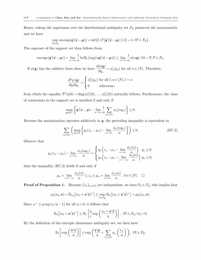
ec4 e-companion to Chen, Sim, and Xu: Distributionally Robust Optimization with Infinitely Constrained Ambiguity Sets
Hence, taking the supremum over the distributional ambiguity set FE preserves the monotonicity
and we have
supP∈FE
ess sup(q′(z−µ)) = inf{δ | P [q′(z−µ)≤ δ] = 1,∀P∈FE}.
The superset of the support set then follows from
ess sup (q′(z−µ)) = limα→∞
1
αlnEP [exp(αq′(z−µ))]≤ lim
α→∞
1
αφ(αq),∀z ∼ P,P∈FE.
If φ(q) has the additive form then we have∂φ(q)
∂qn= φ′n(qn) for all n∈ [N ]. Therefore,
∂2φ (q)
∂ql∂qn=
φ′′n(qn) for all l, n∈ [N ], l= n
0 otherwise,
from which the equality ∇2φ(0) = diag (φ′′1(0), . . . , φ′′N(0)) naturally follows. Furthermore, the class
of constraints in the support set is satisfied if and only if
maxq∈RN
{q′(z−µ)− lim
α→∞
1
α
∑n∈[N ]
φn(αqn)
}≤ 0.
Because the maximization operates additively in q, the preceding inequality is equivalent to∑n∈[N ]
(maxqn∈R
{qn(zn−µn)− lim
α→∞
φn(αqn)
α
})≤ 0. (EC.2)
Observe that
qn(zn−µn)− limα→∞
φn(αqn)
α=
qn
(zn−µn− lim
α→∞
φn(α)
α
)qn ≥ 0
qn
(zn−µn− lim
α→−∞
φn(α)
α
)qn ≤ 0,
thus the inequality (EC.2) holds if and only if
µn + limα→−∞
φn(α)
α≤ zn ≤ µn + lim
α→∞
φn(α)
α, ∀n∈ [N ]. �
Proof of Proposition 1. Because {zn}n∈[N ] are independent, we have P0 ∈FE; this implies that
ρ0(x0,x) =EP0
[(x0 +x′z)+
]≤ sup
P∈FEEP[(x0 +x′z)+
]= ρE(x0,x).
Since ω+ ≤ η exp (ω/η− 1) for all η > 0, it follows that
EP[(x0 +x′z)+
]≤EP
[η
eexp
(x0 +x′z
η
)], ∀P∈FE,∀η > 0.
By the definition of the entropic dominance ambiguity set, we then have
EP
[exp
(x′z
η
)]≤ exp
(x′µ
η+∑n∈[N ]
φn
(xnη
)), ∀P∈FE.
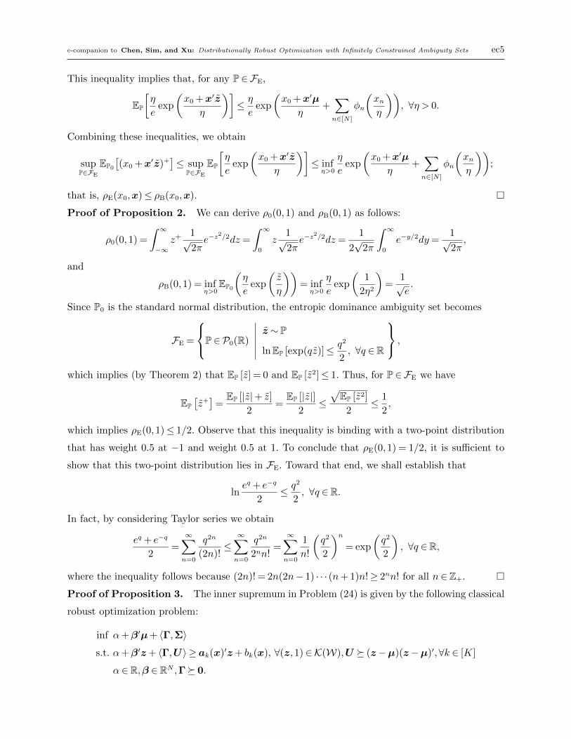
e-companion to Chen, Sim, and Xu: Distributionally Robust Optimization with Infinitely Constrained Ambiguity Sets ec5
This inequality implies that, for any P∈FE,
EP
[η
eexp
(x0 +x′z
η
)]≤ η
eexp
(x0 +x′µ
η+∑n∈[N ]
φn
(xnη
)), ∀η > 0.
Combining these inequalities, we obtain
supP∈FE
EP0
[(x0 +x′z)+
]≤ sup
P∈FEEP
[η
eexp
(x0 +x′z
η
)]≤ inf
η>0
η
eexp
(x0 +x′µ
η+∑n∈[N ]
φn
(xnη
));
that is, ρE(x0,x)≤ ρB(x0,x). �
Proof of Proposition 2. We can derive ρ0(0,1) and ρB(0,1) as follows:
ρ0(0,1) =
∫ ∞−∞
z+ 1√2πe−z
2/2dz =
∫ ∞0
z1√2πe−z
2/2dz =1
2√
2π
∫ ∞0
e−y/2dy=1√2π,
and
ρB(0,1) = infη>0
EP0
(η
eexp
(z
η
))= inf
η>0
η
eexp
(1
2η2
)=
1√e.
Since P0 is the standard normal distribution, the entropic dominance ambiguity set becomes
FE =
P∈P0(R)
∣∣∣∣∣∣z ∼ P
lnEP [exp(qz)]≤ q2
2, ∀q ∈R
,
which implies (by Theorem 2) that EP [z] = 0 and EP [z2]≤ 1. Thus, for P∈FE we have
EP[z+]
=EP [|z|+ z]
2=
EP [|z|]2≤√EP [z2]
2≤ 1
2,
which implies ρE(0,1)≤ 1/2. Observe that this inequality is binding with a two-point distribution
that has weight 0.5 at −1 and weight 0.5 at 1. To conclude that ρE(0,1) = 1/2, it is sufficient to
show that this two-point distribution lies in FE. Toward that end, we shall establish that
lneq + e−q
2≤ q2
2, ∀q ∈R.
In fact, by considering Taylor series we obtain
eq + e−q
2=∞∑n=0
q2n
(2n)!≤∞∑n=0
q2n
2nn!=∞∑n=0
1
n!
(q2
2
)n= exp
(q2
2
), ∀q ∈R,
where the inequality follows because (2n)! = 2n(2n− 1) · · · (n+ 1)n!≥ 2nn! for all n∈Z+. �
Proof of Proposition 3. The inner supremum in Problem (24) is given by the following classical
robust optimization problem:
inf α+β′µ+ 〈Γ,Σ〉
s.t. α+β′z+ 〈Γ,U〉 ≥ ak(x)′z+ bk(x), ∀(z,1)∈K(W),U � (z−µ)(z−µ)′,∀k ∈ [K]
α∈R,β ∈RN ,Γ� 0.

ec6 e-companion to Chen, Sim, and Xu: Distributionally Robust Optimization with Infinitely Constrained Ambiguity Sets
Here we have introduced the auxiliary variable U ∈RN×N and represent the constraint z ∈W by
(z,1) ∈ K(W). Using the Schur complement, we know that each k-th robust counterpart is not
violated if and only if
inf (β−ak(x))′z+ 〈Γ,U〉
s.t.
1 (z−µ)′
(z−µ) U
� 0
(z,1)∈KW
is not less than bk(x)−α. The dual of the above problem is
sup 2χ′kµ− δk− tks.t. β−ak(x)− rk− 2χk = 0
Γ = Γk
(rk, tk)∈K∗W δk χ′kχk Γk
� 0.
Substituting this dual formulation and then performing the outer and inner minimizations jointly,
we obtain the formulation (25). �
Proof of Proposition 4. The inner supremum in Problem (27) can be reformulated as
inf α+β′µ+∑j∈[J]
γjq′jΣqj
s.t. α+β′z+∑j∈[J]
γj(q′j(z−µ))2 ≥ ak(x)′z+ bk(x), ∀(z,1)∈K(W),∀k ∈ [K]
α∈R,β ∈RN ,γ ∈RJ+.
In this formulation, each k-th constraint is not violated if and only if the optimal value of the
problem
inf (β−ak(x))′z+γ ′u
s.t. uj ≥(q′j(z−µ)
)2, ∀j ∈ [J ]
(z,1)∈W
is not less than bk(x) − α. Here, we have introduced an auxiliary vector u such that the uj is
associated with the epigraph of quadratic function(q′j(z−µ)
)2. The first set of constraints has an
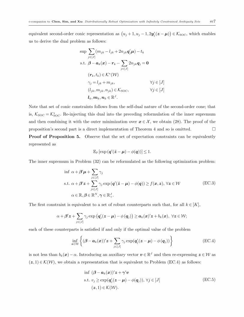
e-companion to Chen, Sim, and Xu: Distributionally Robust Optimization with Infinitely Constrained Ambiguity Sets ec7
equivalent second-order conic representation as(uj + 1, uj − 1,2y′j(z−µ)
)∈ KSOC, which enables
us to derive the dual problem as follows:
sup∑j∈[J]
(mjk− ljk + 2njkq′jµ)− tk
s.t. β−ak(x)− rk−∑j∈[J]
2njkqj = 0
(rk, tk)∈K∗(W)
γj = ljk +mjk, ∀j ∈ [J ]
(ljk,mjk, njk)∈KSOC, ∀j ∈ [J ]
lk,mk,nk ∈RJ .
Note that set of conic constraints follows from the self-dual nature of the second-order cone; that
is, KSOC = K∗SOC. Re-injecting this dual into the preceding reformulation of the inner supremum
and then combining it with the outer minimization over x ∈ X , we obtain (28). The proof of the
proposition’s second part is a direct implementation of Theorem 4 and so is omitted. �
Proof of Proposition 5. Observe that the set of expectation constraints can be equivalently
represented as
EP [exp (q′(z−µ)−φ(q))]≤ 1.
The inner supremum in Problem (32) can be reformulated as the following optimization problem:
inf α+β′µ+∑j∈[J]
γj
s.t. α+β′z+∑j∈[J]
γj exp (q′(z−µ)−φ(q))≥ f(x,z), ∀z ∈W
α∈R,β ∈RN ,γ ∈RJ+.
(EC.3)
The first constraint is equivalent to a set of robust counterparts such that, for all k ∈ [K],
α+β′z+∑j∈[J]
γj exp(q′j(z−µ)−φ (qj)
)≥ ak(x)′z+ bk(x), ∀z ∈W;
each of these counterparts is satisfied if and only if the optimal value of the problem
infz∈W
{(β−ak(x))′z+
∑j∈[J]
γj exp(q′j(z−µ)−φ (qj))
}(EC.4)
is not less than bk(x)−α. Introducing an auxiliary vector v ∈RJ and then re-expressing z ∈W as
(z,1)∈K(W), we obtain a representation that is equivalent to Problem (EC.4) as follows:
inf (β−ak(x))′z+γ ′v
s.t. vj ≥ exp(q′j(z−µ)−φ(qj)), ∀j ∈ [J ]
(z,1)∈K(W).
(EC.5)
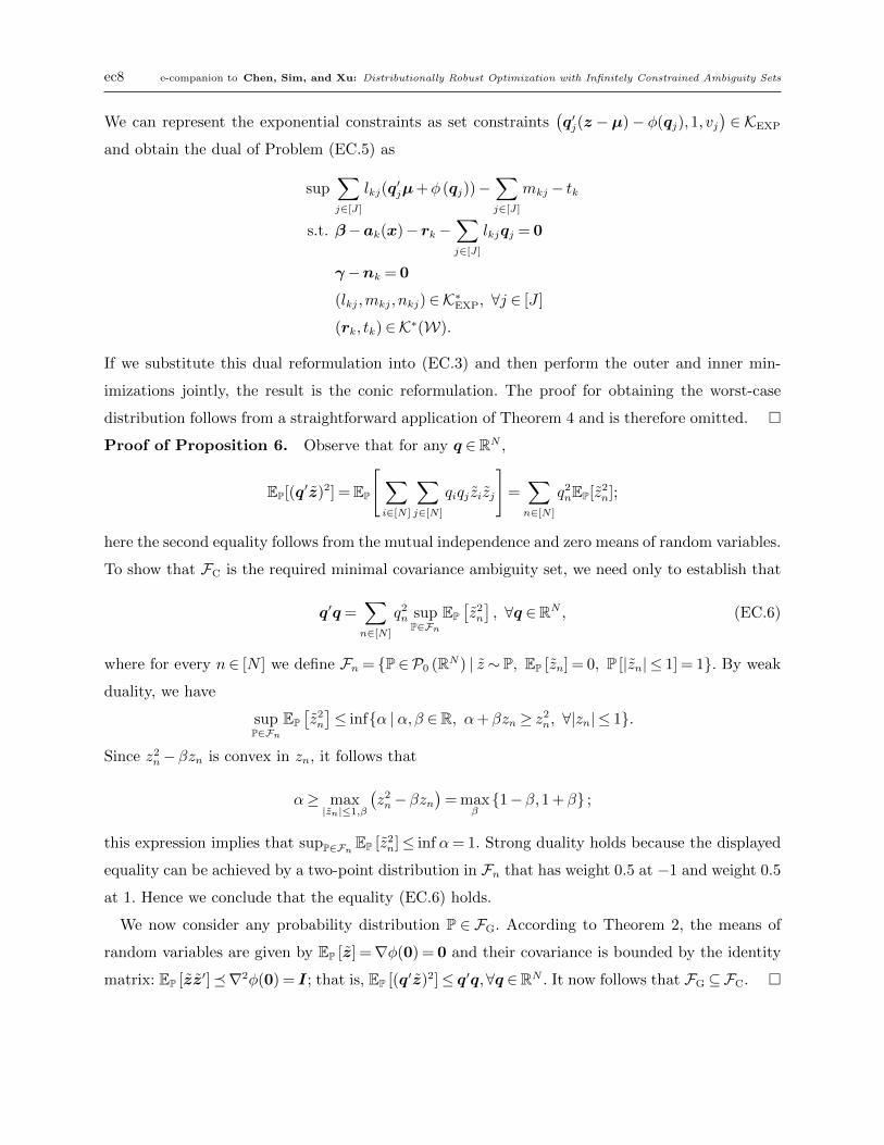
ec8 e-companion to Chen, Sim, and Xu: Distributionally Robust Optimization with Infinitely Constrained Ambiguity Sets
We can represent the exponential constraints as set constraints(q′j(z −µ)− φ(qj),1, vj
)∈ KEXP
and obtain the dual of Problem (EC.5) as
sup∑j∈[J]
lkj(q′jµ+φ (qj))−
∑j∈[J]
mkj − tk
s.t. β−ak(x)− rk−∑j∈[J]
lkjqj = 0
γ−nk = 0
(lkj,mkj, nkj)∈K∗EXP, ∀j ∈ [J ]
(rk, tk)∈K∗(W).
If we substitute this dual reformulation into (EC.3) and then perform the outer and inner min-
imizations jointly, the result is the conic reformulation. The proof for obtaining the worst-case
distribution follows from a straightforward application of Theorem 4 and is therefore omitted. �
Proof of Proposition 6. Observe that for any q ∈RN ,
EP[(q′z)2] =EP
[ ∑i∈[N ]
∑j∈[N ]
qiqj zizj
]=∑n∈[N ]
q2nEP[z2
n];
here the second equality follows from the mutual independence and zero means of random variables.
To show that FC is the required minimal covariance ambiguity set, we need only to establish that
q′q=∑n∈[N ]
q2n supP∈Fn
EP[z2n
], ∀q ∈RN , (EC.6)
where for every n∈ [N ] we define Fn = {P∈P0 (RN) | z ∼ P, EP [zn] = 0, P [|zn| ≤ 1] = 1}. By weak
duality, we have
supP∈Fn
EP[z2n
]≤ inf{α | α,β ∈R, α+βzn ≥ z2
n, ∀|zn| ≤ 1}.
Since z2n−βzn is convex in zn, it follows that
α≥ max|zn|≤1,β
(z2n−βzn
)= max
β{1−β,1 +β} ;
this expression implies that supP∈Fn EP [z2n]≤ inf α= 1. Strong duality holds because the displayed
equality can be achieved by a two-point distribution in Fn that has weight 0.5 at −1 and weight 0.5
at 1. Hence we conclude that the equality (EC.6) holds.
We now consider any probability distribution P ∈ FG. According to Theorem 2, the means of
random variables are given by EP [z] =∇φ(0) = 0 and their covariance is bounded by the identity
matrix: EP [zz′]�∇2φ(0) = I; that is, EP [(q′z)2]≤ q′q,∀q ∈RN . It now follows that FG ⊆FC. �