DISTRIBUTIONAL INCENTIVES IN AN EQUILIBRIUM MODEL OF ... · Distributional Incentives in an...

NBER WORKING PAPER SERIES

DISTRIBUTIONAL INCENTIVES IN AN EQUILIBRIUM MODEL OF DOMESTICSOVEREIGN DEFAULT

Pablo D'ErasmoEnrique G. Mendoza

Working Paper 19477http://www.nber.org/papers/w19477

NATIONAL BUREAU OF ECONOMIC RESEARCH1050 Massachusetts Avenue

Cambridge, MA 02138September 2013

We acknowledge the generous support of the National Science Foundation under awards 1325122and 1324740. Comments by Jesse Schreger, Fabrizio Perri, Vincenzo Quadrini and by participantsat presentations in Columbia University, the 2014 Winter Meetings of the Econometric Society, andthe NBER Conference on Sovereign Debt and Financial Crises are also gratefully acknowledged. Wethank Jingting Fan for excellent research assistance. The views expressed in this paper do not necessarilyreflect those of the Federal Reserve Bank of Philadelphia, the Federal Reserve System, or the NationalBureau of Economic Research.

NBER working papers are circulated for discussion and comment purposes. They have not been peer-reviewed or been subject to the review by the NBER Board of Directors that accompanies officialNBER publications.

© 2013 by Pablo D'Erasmo and Enrique G. Mendoza. All rights reserved. Short sections of text, notto exceed two paragraphs, may be quoted without explicit permission provided that full credit, including© notice, is given to the source.

Distributional Incentives in an Equilibrium Model of Domestic Sovereign DefaultPablo D'Erasmo and Enrique G. MendozaNBER Working Paper No. 19477September 2013, Revised July 2015JEL No. E44,E6,F34,H63

ABSTRACT

Europe’s debt crisis resembles historical episodes of outright default on domestic public debt aboutwhich little research exists. This paper proposes a theory of domestic sovereign default based on distributionalincentives affecting the welfare of risk-averse debt- and non-debt holders. A utilitarian governmentcannot sustain debt if default is costless. If default is costly, debt with default risk is sustainable, anddebt falls as concentration of debt ownership rises. A government favoring bond holders can also sustaindebt, with debt rising as ownership becomes more concentrated. These results are robust to addingforeign investors, redistributive taxes, or a second asset.

Pablo D'ErasmoFederal Reserve Bank of PhiladelphiaResearch DepartmentTen Independence Mall, Philadelphia PA [email protected]

Enrique G. MendozaDepartment of EconomicsUniversity of Pennsylvania3718 Locust WalkPhiladelphia, PA 19104and [email protected]

1 Introduction

The seminal study by Reinhart and Rogoff (2011) identified 68 episodes in which governments

defaulted outright (i.e. by means other than inflation) on their domestic creditors in a cross-

country database going back to 1750. These domestic defaults occurred via mechanisms such

as forcible conversions, lower coupon rates, unilateral reductions of principal, and suspensions

of payments. Reinhart and Rogoff also documented that domestic public debt accounts for a

large fraction of total government debt in the majority of countries (about 2/3rds on average),

and that domestic defaults were associated with periods of severe financial turbulence, which

often included defaults on external debt, banking system collapses and full-blown economic

crises. Despite of these striking features, they also found that domestic sovereign default is a

“forgotten history” that remains largely unexplored in economic research.

The ongoing European debt crisis also highlights the importance of studying domestic

sovereign default. In particular, four features of this crisis make it more akin to a domestic

default than to the typical external default that dominates the literature on public debt default.

First, countries in the Eurozone are highly integrated, with the majority of their public debt

denominated in their common currency and held by European residents. Hence, from an Euro-

pean standpoint, default by one or more Eurozone governments means a suspension of payments

to “domestic” agents, instead of external creditors. Second, domestic public debt-GDP ratios

are high in the Eurozone in general, and very large in the countries at the epicenter of the

crisis (Greece, Ireland, Italy, Spain and Portugal). Third, the Eurozone’s common currency and

common central bank rule out the possibility of individual governments resorting to inflation as

a means to lighten their debt burden without an outright default. Fourth, and perhaps most

important from the standpoint of the theory proposed in this paper, European-wide institutions

such as the ECB and the European Commission are weighting the interests of both creditors

and debtors in assessing the pros and cons of sovereign defaults by individual countries, and

creditors and debtors are aware of these institutions’ concern and of their key role in influencing

expectations and default risk.1 Hall and Sargent (2014) document a similar situation in the

process by which the U.S. government handled the management of its debt in the aftermath of

the Revolutionary War.

Table 1 shows that the Eurozone fiscal crisis has been characterized by rapid increases in

public debt ratios and sovereign spreads that coincided with rising government expenditure

ratios. The Table also shows that debt ownership, as proxied by Gini coefficients of wealth

distributions, is unevenly distributed in the seven countries listed, with mean and median Gini

1The analogy with a domestic default is imperfect, however, because the Eurozone is not a single country,and in particular there is no fiscal entity with tax and debt-issuance powers over all the members.

2

coefficients of around 2/3rds.2

Table 1: Euro Area: Key Fiscal Statistics and Wealth Inequality

Gov. Debt Gov. Exp. Spreads GiniMoment (%) Avg. 2011 Avg. “crisis peak” Avg. “crisis peak” WealthFrance 34.87 62.72 23.40 24.90 0.08 1.04 0.73Germany 33.34 52.16 18.80 20.00 - - 0.67Greece 84.25 133.09 18.40 23.60 0.37 21.00 0.65Ireland 14.07 64.97 16.10 20.50 0.11 6.99 0.58Italy 95.46 100.22 19.40 21.40 0.27 3.99 0.61Portugal 35.21 75.83 20.00 22.10 0.20 9.05 0.67Spain 39.97 45.60 17.60 21.40 0.13 4.35 0.57Avg. 48.17 76.37 19.10 21.99 0.22 7.74 0.64Median 35.21 64.97 18.80 21.40 0.17 5.67 0.65

Note: Author’s calculations based on OECD Statistics, Eurostat, ECSB and

Davies, Sandstrm, Shorrocks, and Wolff (2009). “Gov. Debt” refers to Total General Government Net

Financial Liabilities (avg 90-07); “Gov. Exp.” corresponds to government purchases in National Accounts (avg

00-07); “Sov Spreads” correspond to the difference between interest rates of the given country and Germany

for bonds of similar maturity (avg 00-07). For a given country i, they are computed as (1+ri)(1+rGer) − 1. “Crisis

Peak” refers to the maximum value observed during 2008-2012 using data from Eurostat. “Gini Wealth” are

Gini wealth coefficients for 2000 from Davies, Sandstrm, Shorrocks, and Wolff (2009) Appendix V.

Taken together, the history of domestic defaults and the risk of similar defaults in Europe

pose two important questions: What explains the existence of domestic debt ratios exposed to

default risk? And, can the concentration of the ownership of government debt be a determinant

of domestic debt exposed to default risk?

This paper aims to answer these questions by proposing a framework for explaining domestic

sovereign defaults driven by distributional incentives. This framework is motivated by the key

fact that a domestic default entails substantial redistribution across domestic agents, with all of

these agents, including government debt holders, entering in the payoff function of the sovereign.

This is in sharp contrast with what standard models of external sovereign default assume,

particularly those based on the classic work of Eaton and Gersovitz (1981).

We propose a tractable two-period model with heterogeneous agents and non-insurable aggre-

gate risk in which domestic default can be optimal for a government responding to distributional

incentives. A fraction γ of agents are low-wealth (L) agents who do not hold government debt,

2In Section A.1 of the Appendix, we present a more systematic analysis of the link between debt and inequalityand show that government debt is increasing in inequality when inequality is low but decreasing for high levelsof inequality.

3

and a fraction 1 − γ are high-wealth (H) agents who hold the debt. The government finances

the gap between exogenous stochastic expenditures and endogenous taxes by issuing non-state-

contingent debt, retaining the option to default. In our benchmark case, the government is

utilitarian,, so the social welfare function assigns the weights γ and 1 − γ to the welfare of L

and H agents respectively.

If the government is utilitarian and default is costless, the model cannot support an equi-

librium with debt. This is because for any given level of debt that could have been issued in

the first period, the government always attains the second period’s socially efficient levels of

consumption allocations and redistribution by choosing to default, and if default in period two

is certain the debt market collapses in the first period. An equilibrium with debt under a utili-

tarian government can exist if default entails an exogenous cost in terms of disposable income.

When default is costly, repayment becomes optimal if the amount of period-two consumption

dispersion that the competitive equilibrium with repayment supports yields higher welfare than

the default equilibrium net of default cost.

Alternatively, we show that an equilibrium with debt can be supported if the government’s

payoff function displays a “political” bias in favor of bond holders, even if default is costless.

In this case, the government’s weight on H-type agents is higher than the actual fraction of

these agents in the distribution of bond holdings. In this extension, the debt is an increasing

function of the concentration of debt ownership, instead of decreasing as in the utilitarian case.

This is because incentives to default get weaker as the government’s weight on L-type agents

falls increasingly below γ. The model with political bias also yields the interesting result that

agents that do not hold public debt may prefer a government that weighs bond holders more

than a utilitarian government. This is because the government with political bias has weaker

default incentives, and can thus sustain higher debt at lower default probabilities, which relaxes

a liquidity constraint affecting agents who do not hold public debt by improving tax smoothing.

We also explore other three important extensions of the model to show that the main result

of the benchmark model, namely the existence of equilibria with domestic public debt exposed

to default risk, is robust. We examine extensions opening the economy so that a portion of the

debt is held by foreign investors, introducing taxation as another instrument for redistributive

policy, and adding a second asset as an alternative vehicle for saving.

This work is related to various strands of the large literature on public debt. First, studies

on public debt as a self-insurance mechanism and a vehicle that alters consumption disper-

sion in heterogeneous agents models without default, such as Aiyagari and McGrattan (1998),

Golosov and Sargent (2012), Azzimonti, de Francisco, and Quadrini (2014), Floden (2001) and

4

Heathcote (2005).3

A second strand is the literature on external sovereign default in the line of the Eaton and Gersovitz

(1981) model (e.g. Aguiar and Gopinath (2006), Arellano (2008), Pitchford and Wright (2012),

Yue (2010)).4 Also in this literature, and closely related, Aguiar and Amador (2013) analyze

the interaction between public debt, taxes and default risk and Lorenzoni and Werning (2013)

study the dynamics of debt and interest rates in a model where default is driven by insolvency

and debt issuance follows a fiscal rule.

A third strand is the literature on political economy and sovereign default, which also fo-

cuses mostly on external default (e.g. Amador (2003), Dixit and Londregan (2000), D’Erasmo

(2011), Guembel and Sussman (2009), Hatchondo, Martinez, and Sapriza (2009) and Tabellini

(1991)). A few studies like those of Alesina and Tabellini (1990) and Aghion and Bolton (1990)

do focus on political economy aspects of government debt in a closed economy, including default,

and Aguiar, Amador, Farhi, and Gopinath (2013) examine optimal policy in a monetary union

subject to self-fulfilling debt crises.

A fourth important strand of the literature focuses on the consequences of default on domestic

agents, the role of secondary markets, discriminatory v. nondiscriminatory default and the role of

domestic debt in providing liquidity (see Guembel and Sussman (2009), Broner, Martin, and Ventura

(2010), Broner and Ventura (2011), Gennaioli, Martin, and Rossi (2014), Basu (2009), Brutti

(2011), Mengus (2014) and Di Casola and Sichlimiris (2014)).5 As in most of these studies, de-

fault in our setup is non-discriminatory, because the government cannot discriminate across any

of its creditors when it defaults. Our analysis differs in that default is driven by distributional

incentives.6

Finally, there is also a newer literature that is closer to our work in that it studies the trade-

offs between distributional incentives to default on domestic debt and the use of debt in infinite-

horizon models with heterogeneous agents (see, in particular, D’Erasmo and Mendoza (2014)

and Dovis, Golosov, and Shourideh (2014)). In D’Erasmo and Mendoza, debt is determined by

3A related literature initiated by Aiyagari, Marcet, Sargent, and Seppala (2002) studies optimal taxationand public debt dynamics with aggregate uncertainty and incomplete markets, but in a representative-agentenvironment. Pouzo and Presno (2014) extended this framework to incorporate default and renegotiation.

4See Panizza, Sturzenegger, and Zettelmeyer (2009), Aguiar and Amador (2014), and Tomz and Wright(2012) for recent reviews of the sovereign debt literature. Some studies in this area have examined modelsthat include tax and expenditure policies, as well as settings with foreign and domestic lenders, but always main-taining the representative agent assumption (e.g. Cuadra, Sanchez, and Sapriza (2010)), Vasishtha (2010) andmore recently Dias, Richmond, and Wright (2012) have examined the benefits of debt relief from the perspectiveof a global social planner with utilitarian preferences.

5Motivated by the recent financial crisis and extending the theoretical work of Gennaioli, Martin, and Rossi(2014), a set of recent papers focuses on the interaction between sovereign debt and domestic financial institutions,such as Sosa-Padilla (2012), Bocola (2014), Boz, D’Erasmo, and Durdu (2014) and Perez (2015).

6Andreasen, Sandleris, and der Ghote (2011), Ferriere (2014) and Jeon and Kabukcuoglu (2014) study envi-ronments in which domestic income heterogeneity plays a central role in the determination of external defaults.

5

a fiscal rule, while in this paper we model public debt as an optimal choice and derive analytical

expressions that characterize equilibrium prices and the solution of the government’s problem.

Our work differs from Dovis et al. in that they assume complete domestic asset markets, so

their analysis abstracts from the role of public debt in providing social insurance, while the

non-state-contingent nature of public debt plays a central role in the distributional incentives

we examine here and in the endogenous default costs studied in D’Erasmo and Mendoza (2014).

In addition, Dovis et al. focus on the solution to a Ramsey problem that supports equilibria

in which default is not observed along the equilibrium path, while in our work default is an

equilibrium outcome.7

2 Model Environment

Consider a two-period economy inhabited by a continuum of agents with aggregate unit mea-

sure. Agents differ in their initial wealth position, which is characterized by their holdings of

government debt at the beginning of the first period. The government is represented by a social

planner with a utilitarian payoff who issues one-period, non-state-contingent debt, levies lump-

sum taxes, and has the option to default. Government debt is the only asset available in the

economy and is entirely held by domestic agents.

2.1 Household Preferences & Budget Constraints

All agents have the same preferences, which are given by:

u(c0) + βE[u(c1)], u(c) =c1−σ

1− σ

where β ∈ (0, 1) is the discount factor and ct for t = 0, 1 is individual consumption. The utility

function u(·) takes the standard CRRA form.

All agents receive a non-stochastic endowment y each period and pay lump-sum taxes τt,

which are uniform across agents. Taxes and newly issued government debt are used to pay

for government consumption gt and repayment of outstanding government debt. The initial

supply of outstanding government bonds at t = 0 is denoted B0. Given B0, the initial wealth

distribution is defined by a fraction γ of households who are the L-type individuals with initial

bond holdings bL0 , and a fraction (1 − γ) who are the H-types and hold bH0 > bL0 . These initial

bond holdings satisfy market clearing: γbL0 + (1− γ)bH0 = B0, which given bH0 > bL0 implies that

bH0 > B0 and bL0 < B0.

7See also Golosov and Sargent (2012) who study debt dynamics without default risk in a similar environment.

6

The budget constraints of the two types of households in the first period are given by:

ci0 + q0bi1 = y + bi0 − τ0 for i = L,H. (1)

Agents collect the payout on their initial holdings of government debt (bi0), receive endowment

income y, and pay lump-sum taxes τ0. This net-of-tax resources are used to pay for consumption

and purchases of new government bonds bi1 at price q0. Agents are not allowed to take short

positions in government bonds, which is equivalent to imposing the no-borrowing condition often

used in heterogeneous-agents models with incomplete markets: bi1 ≥ 0.

The budget constraints in the second period differ depending on whether the government

defaults or not. If the government repays, the budget constraints take the standard form:

ci1 = y + bi1 − τ1 for i = L,H. (2)

If the government defaults, there is no repayment on the outstanding debt, and the agents’

budget constraints are:

ci1 = (1− φ(g1))y − τ1 for i = L,H. (3)

As is standard in the sovereign debt literature, we can allow for default to impose an exogenous

cost that reduces income by a fraction φ. This cost is usually modeled as a function of the

realization of a stochastic endowment income, but since income is constant in this setup, we

model it as a function of the realization of government expenditures in the second period g1.

In particular, the cost is a non-increasing, step-wise function: φ(g1) ≥ 0, with φ′(g1) ≤ 0 for

g1 ≤ g1, φ′(g1) = 0 otherwise, and φ′′(g1) = 0. Hence, g1 is a threshold high value of g1 above

which the marginal cost of default is zero.8

2.2 Government

At the beginning of t = 0, the government has outstanding debt B0 and can issue one-period,

non-state contingent discount bonds B1 ∈ B ≡ [0,∞) at the price q0 ≥ 0. Each period, the

government collects lump-sum revenues τt and pays for gt. Since g0 is known at the beginning

of the first period, the relevant uncertainty with respect to government expenditures is for g1,

8This formulation is analogous to the step-wise default cost as a function of income proposed by Arellano(2008) and now widely used in the external default literature, and it also captures the idea of asymmetric costsof tax collection (see Barro (1979) and Calvo (1988)). Note, however, that for the model to support equilibriawith debt under a utilitarian government all we need is φ(g1) > 0. The additional structure is useful for thequantitative analysis and for making it easier to compare the model with the standard external default models.In external default models, the non-linear cost makes default more costly in “good” states, which alters defaultincentives to make default more frequent in “bad” states, and it also contributes to support higher debt levels.

7

which is characterized by a well-defined probability distribution function with mean µg. We do

not restrict the sign of τt, so τt < 0 represents lump-sum transfers.

At equilibrium, the price of debt issued in the first period must be such that the government

bond market clears:

Bt = γbLt + (1− γ)bHt for t = 0, 1. (4)

This condition is satisfied by construction in period 0. In period 1, however, the price moves

endogenously to clear the market.

The government has the option to default at t = 1. The default decision is denoted by

d1 ∈ {0, 1} where d1 = 0 implies repayment. The government evaluates the values of repayment

and default as a benevolent planner with a social welfare function. In the rest of this Section we

focus on the case of a standard utilitarian social welfare function: γu(cL1 ) + (1 − γ)u(cH1 ). The

government, however, cannot discriminate across the two types of agents when setting taxation,

debt and default policies.

At t = 0, the government budget constraint is

τ0 = g0 +B0 − q0B1. (5)

The level of taxes in period 1 is determined after the default decision. If the government

repays, taxes are set to satisfy the following government budget constraint:

τd1=01 = g1 +B1. (6)

Notice that, since this is a two-period model, equilibrium requires that there are no outstanding

assets at the end of period 1 (i.e. bi2 = B2 = 0 and q1 = 0). If the government defaults, taxes

are simply set to pay for government purchases:

τd1=11 = g1. (7)

3 Equilibrium

The analysis of the model’s equilibrium proceeds in three stages. First, we characterize the

households’ optimal savings problem and determine their payoff (or value) functions, taking as

given the government debt, taxes and default decision. Second, we study how optimal govern-

ment taxes and the default decision are determined. Third, we examine the optimal choice of

debt issuance that internalizes the outcomes of the first two stages.

8

3.1 Households’ Problem

Given B1 and γ, a household with initial debt holdings bi0 for i = L,H chooses bi1 by solving

this maximization problem:

vi(B1, γ) = maxbi1

{u(y + bi0 − q0(B1, γ)b

i1 − τ0) + (8)

βEg1

[(1− d1(B1, g1, γ))u(y + bi1 − τd1=0

1 ) + d1(B1, g1, γ)u(y(1− φ(g1))− τd1=11 )

]},

subject to bi1 ≥ 0. The term Eg1 [.] represents the expected payoff across the repayment and

default states in period 1.9

The first-order condition, evaluated at the equilibrium level of taxes, yields the following

Euler equation:

u′(ci0) ≥ β(1/q0(B1, γ))Eg1

[u′(y − g1 + bi1 − B1)(1− d1(B1, g1, γ))

], = if bi1 > 0 (9)

In states in which, given (B1, γ), the value of g1 is such that the government chooses to default

(d1(B1, g1, γ) = 1), the marginal benefit of an extra unit of debt is zero.10 Thus, conditional

on B1, a larger default set (i.e. a larger set of values of g1 such that the government defaults),

implies that the expected marginal benefit of an extra unit of savings decreases. This implies

that, everything else equal, a higher default probability results in a lower demand for government

bonds, a lower equilibrium bond price, and higher taxes.11

Given that income and taxes are homogeneous across agents, it has to be the case at equi-

librium that bH1 > bL1 , which therefore implies that H−types are never credit constrained. In

contrast, whether L − types are credit constrained or not depends on parameter values. This

is less likely to happen the higher bL0 , B0 or B1. Whenever the L−types are constrained, the

H−types are the marginal investor and their Euler equation can be used to derive the equi-

librium price. For the remainder of the paper we focus on equilibria in which L−types are

constrained (i.e. bL0 = bL1 = 0), in order to capture the feature of heterogeneous agents models

with incomplete markets that a fraction of agents is always credit constrained endogenously, and

public debt has the social benefit that it contributes to reduce the tightness of this constraint.

The equilibrium bond price is the value of q0(B1, γ) for which, as long as consumption for all

agents is non-negative and the default probability of the government is less than 1, the following

9Notice in particular that the payoff in case of default does not depend on the level of individual debt holdings(bi1), reflecting the fact that the government cannot discriminate across households when it defaults.

10Utility in the case of default equals u(y(1− φ(g1))− g1), and is independent of bi1.11Note also that from the agents’ perspective, their bond decisions do not affect d1(B1, g1, γ).

9

market-clearing condition holds:

B1 = γbL1 (B1, γ) + (1− γ)bH1 (B1, γ), (10)

where B1 in the left-hand-side of this expression represents the supply of public debt, and the

right-hand-side is the aggregate government bond demand.

It is instructive to analyze further the households’ problem assuming logarithmic utility

(u(c) = log(c)), because under these assumptions we can solve for q0(B1, γ) in closed form, and

use the solution to establish some important properties of bond prices and default risk spreads.

We show in Section A.4 of the Appendix that the equilibrium bond price is:

q0(B1, γ) = β

(y − g0 +

(γ

1−γ

)B0

)Π(B1, γ)

1 +(

γ

1−γ

)βB1Π(B1, γ),

(11)

where Π(B1, γ) ≡ Eg1

[1−d(B1,g1,γ)

y−g1+( γ

1−γ )B1

]is the expected marginal utility of H−type agents for the

second period, which weights only non-default states because the marginal benefit of debt is zero

in default states. Since, as also shown in the Appendix (Section A.4), ∂Π(B1,γ)∂B1

< 0, it follows

that ∂q0(B1,γ)∂B1

< 0 for cH0 > 0. Moreover, since bond prices are decreasing in B1, it follows that

the “revenue” the government generates by selling debt, q0(B1, γ)B1, behaves like the familiar

debt Laffer curve of the Eaton-Gersovitz models derived by Arellano (2008).12 This Laffer curve

will play a key role later in determining the government’s optimal debt choice. In particular, the

government internalizes that higher debt eventually produces decreasing revenues, and that in

the decreasing segment of the Laffer curve revenues fall faster as the debt increases, and much

faster as default risk rises sharply.

A similar expression can be obtained for the “risk-free” price (i.e., the bond price that arises

in a model with full commitment), to show that the risk premium is non-negative, and it is

strictly positive if there is default in equilibrium. The premium is increasing in B1 since the

default set is increasing in B1. We also show in Section A.4 of the Appendix that the spread

is a multiple of 1/β(y − g0 +

(γ

1−γ

)B0

). As a result, the total date-0 resources available for

consumption of the H-types (y − g0 +(

γ

1−γ

)B0) have a first-order negative effect on default

risk spreads. This is because, as this measure of income rises, the marginal utility of date-0

consumption of H types falls, which pushes up bond prices. Changes in γ have a similar impact

12It is straightforward to show that revenue R(B1) = q0(B1, γ)B1 follows a Laffer curve in the [0, Bmax1 ]

interval, where Bmax1 is the upper bound of debt such that the government chooses default for any realization

of g1 and thus q0(Bmax1 , γ) = 0. Since R(0) = 0 with R′(0) = q(0, γ) > 0, and R(Bmax

1 ) = 0 with R′(Bmax1 ) =

q′0(Bmax1 , γ)Bmax

1 < 0, it follows by Rolle’s theorem that R(B1) has at least one local maximum in (0, Bmax1 ).

10

on this ratio also pushing spreads downward. However, as γ increases default incentives also

strengthen, as the welfare of debt holders is valued less. Thus, in principle the response of

spreads to increases in the concentration of debt ownership is ambiguous.

3.2 Government’s Problem

3.2.1 Government Default Decision at t = 1

At t = 1, the government chooses to default or not by solving this optimization problem:

maxd∈{0,1}

{W d=0

1 (B1, g1, γ),Wd=11 (g1)

}, (12)

where W d=01 (B1, g1, γ) and W d=1

1 (g1) denote the values of the social welfare function at the

beginning of period 1 in the case of repayment and default respectively. Using the government

budget constraint to substitute for τd=01 and τd=1

1 , the government’s utilitarian payoffs can be

expressed as:

W d=01 (B1, g1, γ) = γu(y − g1 + bL1 − B1) + (1− γ)u(y − g1 + bH1 − B1) (13)

and

W d=11 (g1) = u(y(1− φ(g1))− g1). (14)

Notice that all households lose g1 of their income to government absorption regardless of the

default choice. Moreover, debt repayment reduces consumption and welfare of L types and rises

them for H types (since (bL1 − B1) ≤ 0 and (bH1 − B1) ≥ 0), whereas default implies the same

consumption and utility for both types of agents.

The distributional mechanism determining the default decision can be illustrated by means

of a graphical tool. To this end, it is helpful to express the values of optimal debt holdings

as bL1 = B1 − ǫ and bH1 (γ) = B1 + γ

1−γǫ, for some hypothetical decentralized allocation of

debt holdings given by ǫ ∈ [0, B1]. Consumption allocations under repayment would therefore

be cL1 (ǫ) = y − g1 − ǫ and cH1 (γ, ǫ) = y − g1 +γ

1−γǫ, so ǫ also determines the decentralized

consumption dispersion. The efficient dispersion of consumption that the social planner would

choose is characterized by the value of ǫSP that maximizes social welfare under repayment, which

satisfies this first-order condition:

u′

(y − g1 +

γ

1− γǫSP)

= u′(y − g1 − ǫSP

). (15)

Hence, the efficient allocations are characterized by zero consumption dispersion, because equal

11

marginal utilities imply cL,SP=cH,SP = y − g1, which is attained with ǫSP = 0.

Consider now the government’s default decision when default is costless (φ(g1) = 0). This

scenario is depicted in Figure 1, which plots the social welfare function under repayment as a

function of ǫ as the bell-shaped curve, and the social welfare under default (which is independent

of ǫ), as the black dashed line.

Figure 1: Default Decision and Consumption Dispersion

−0.5 −0.4 −0.3 −0.2 −0.1 0 0.1 0.2 0.3 0.4 0.5−1.5

−1.45

−1.4

−1.35

−1.3

−1.25

−1.2

−1.15

−1.1

(ǫ)

W d=0(ǫ)

ǫSP

u(y − g1)

u(y(1− φ)− g1)

ǫ̂

default zone (φ> 0)

default zone (φ= 0)

repayment zone

(φ> 0)

Clearly, the maximum welfare under repayment is attained when ǫ = 0 which is also the

efficient amount of consumption dispersion ǫSP .13 Given that the only policy instruments the

government can use, other than the default decision, are non-state contingent debt and lump-sum

taxes, it is straightforward to conclude that default is always optimal. This is because default

produces identical allocations in a decentralized equilibrium as the socially efficient ones, since

default produces zero consumption dispersion with consumption levels cL=cH = y − g1. This

outcome is invariant to the values of B1, g1 and γ. This result also implies that the model

without default costs cannot support equilibria with domestic debt subject to default risk,

because default is always optimal.

The outcome is very different when default is costly. With φ(g1) > 0, default still yields

zero consumption dispersion, but at lower levels of consumption and therefore utility, since

consumption allocations in the default state become cL=cH = (1− φ(g1))y − g1. This does not

alter the result that the first-best social optimum is ǫSP = 0, but what changes is that default

13Recall also that we defined the relevant range of decentralized consumption dispersion for ǫ > 0, so welfareunder repayment is decreasing in ǫ over the relevant range.

12

can no longer support the consumption allocations of the first best. Hence, there is now a

threshold amount of consumption dispersion in the decentralized equilibrium, ǫ̂(γ), which varies

with γ and such that for ǫ ≥ ǫ̂(γ) default is again optimal, but for lower ǫ repayment is now

optimal. This is because when ǫ is below the threshold, repayment produces a level of social

welfare higher than the one that default yields. Figure 1 also illustrates this scenario.

3.2.2 Government Debt Decision at t = 0

We can now examine how the government chooses the optimal amount of debt to issue in

the initial period. Before studying the government’s optimization problem, it is important to

emphasize that in this model debt is a mechanism for altering consumption dispersion across

agents, both within a period and across periods. In particular, since bL0 = bL1 = 0, consumption

dispersion in each period and repayment state can be written as: cH0 −cL0 = 11−γ

[B0 − q(B1, γ)B1],

cH,d=01 − cL,d=0

1 = 11−γ

B1, and cH,d=11 − cL,d=1

1 = 0. These expressions make it clear that, given B0,

issuing at least some debt (B1 > 0) reduces consumption dispersion at t = 0 compared with no

debt (B1 = 0), but increases it at t = 1 if the government repays (i.e., d = 0). Moreover, the debt

Laffer curve that governs q0(B1, γ)B1 limits the extent to which debt can reduce consumption

dispersion at t = 0. Starting from B1 = 0, consumption dispersion in the initial period falls as

B1 increases, but there is a critical positive value of B1 beyond which it increases with debt.

At t = 0, the government chooses its debt policy internalizing the above effects, including

the dependence of bond prices on the debt issuance choice. The government chooses B1 so as

to maximize the “indirect” social welfare function:

W0(γ) = maxB1

{γvL(B1, γ) + (1− γ)vH(B1, γ)

}. (16)

where vL and vH are the value functions obtained from solving the households’ problems defined

in the Bellman equation (8) taking into account the government budget constraints and the

equilibrium pricing function of bonds.

We can gain some intuition about the solution of this maximization problem by deriving

its first-order condition and re-arranging it as follows (assuming that the relevant functions are

differentiable):

u′(cH0 ) = u′(cL0 ) +η

q(B1, γ)γ

{βEg1 [∆d∆W1] + γµL

}(17)

13

where

η ≡ q(B1, γ)/ (q′(B1, γ)B1) < 0,

∆d ≡ d(B1 + δ, g1, γ)− d(B1, g1, γ) ≥ 0, for δ > 0 small,

∆W1 ≡ W d=11 (g1, γ)−W d=0

1 (B1, g1, γ) ≥ 0,

µL ≡ q(B1, γ)u′(cL0 )− βEg1

[(1− d1)u′(cL1 )

]> 0.

In these expressions, η is the price elasticity of the demand for government bonds, ∆d∆W1

represents the marginal distributional benefit of a default, and µL is the shadow value of the

borrowing constraint faced by L-type agents.

If both types of agents were unconstrained in their bonds’ choice, so that in particular

µL = 0, and if there is no change in the risk of default (or assuming commitment to remove

default risk entirely), so that Eg1 [∆d∆W1] = 0, then the optimality condition simplifies to

u′(cH0 ) = u′(cL0 ). Hence, in this case the social planner issues debt so as to equalize marginal

utilities of consumption across agents at date 0, which requires simply setting B1 to satisfy

q(B1, γ)B1 = B0.

If H-type agents are unconstrained and L-types are constrained (i.e. µL > 0), which is

the scenario we are focusing on, and still assuming no change in default risk or a government

committed to repay, the optimality condition reduces to u′(cH0 ) = u′(cL0 ) +ηµL

q(B1,γ). Since η < 0,

this result implies cL0 < cH0 , because u′(cL0 ) > u′(cH0 ). Thus, the government’s debt choice sets

B1 as needed to maintain an optimal, positive level of consumption dispersion. Moreover, since

optimal consumption dispersion is positive, we can also ascertain that B0 > q(B1, γ)B1, which

using the government budget constraint implies that the government runs a primary surplus at

t = 0. The government borrows resources, but less than it would need in order to eliminate all

consumption dispersion (which requires zero primary balance).

The intuition for the optimality of issuing debt can be presented in terms of tax smoothing

and savings: Date-0 consumption dispersion without debt issuance would be B0/(1 − γ), but

this is more dispersion than what the government finds optimal, because by choosing B1 > 0 the

government provides tax smoothing (i.e. reduces date-0 taxes) for everyone, which in particular

eases the L-type agents credit constraint, and provides also a desired vehicle of savings for H

types. Thus, positive debt increases consumption of L types (since cL0 = y−g0−B0+q(B1, γ)B1),

and reduces consumption of H types (since cH0 = y− g0+(

γ

1−γ

)(B0− q(B1, γ)B1)). But issuing

debt (assuming repayment) also increases consumption dispersion a t = 1, since debt is then

paid with higher taxes on all agents, while H agents collect also the debt repayment. Thus, the

debt is being chosen optimally to trade off the social costs and benefits of reducing (increasing)

14

date-0 consumption and increasing (reducing) date-1 consumption for rich (poor) agents.

In the presence of default risk and if default risk changes near the optimal debt choice, the

term Eg1 [∆d∆W1] enters in the government’s optimality condition with a positive sign, which

means the optimal gap in the date-0 marginal utilities of the two agents widens even more.

Hence, the government’s optimal choice of consumption dispersion for t = 0 is greater than

without default risk, and the expected dispersion for t = 1 is lower, because in some states of

the world the government will choose to default and consumption dispersion would then drop

to zero. Moreover, the debt Laffer curve now plays a central role in the government’s weakened

incentives to borrow, because as default risk rises the price of bonds drops to zero faster and

the resources available to reduce date-0 consumption dispersion peak at lower debt levels. In

short, default risk reduces the government’s ability to use non-state-contingent debt in order to

reduce consumption dispersion.

3.3 Competitive Equilibrium with Optimal Debt & Default Policy

For a given value of γ, a Competitive Equilibrium with Optimal Debt and Default

Policy is a pair of household value functions vi(B1, γ) and decision rules bi(B1, γ) for i = L,H ,

a government bond pricing function q0(B1, γ) and a set of government policy functions τ0(B1, γ),

τd∈{0,1}1 (B1, g1, γ), d(B1, g1, γ), B1(γ) such that:

1. Given the pricing function and government policy functions, vi(B1, γ) and bi1(B1, γ) solve

the households’ problem.

2. q0(B1, γ) satisfies the market-clearing condition of the bond market (equation (10)).

3. The government default decision d(B1, g1, γ) solves problem (12).

4. Taxes τ0(B1, γ) and τd1 (B1, g1, γ) are consistent with the government budget constraints.

5. The government debt policy B1(γ) solves problem (16).

4 Quantitative Analysis

In this Section, we study the model’s quantitative predictions based on a calibration using

European data. The goal is to show whether a reasonable set of parameter values can produce an

equilibrium with debt subject to default risk, and to study how the properties of this equilibrium

change with the model’s key parameters. Since the two-period model is not well suited to account

for the time-series dynamics of the data, we see the results more as an illustration of the potential

15

relevance of the model’s argument for explaining domestic default rather than as an evaluation

of the model’s general ability to match observed public debt dynamics.14

4.1 Calibration

The model is calibrated to annual frequency, and most of the parameter values are set so that the

model matches moments from European data. The calibrated parameter values are summarized

in Table 2. The details of the calibration are available in Section A.5 of the Appendix. Note also

that we assume a log-normal process for g1, so that ln(g1) ∼ N((1− ρg) ln(µg) + ρg ln(g0),

σ2e

(1−ρ2g)

).15

and the cost of default takes the following functional form: φ(g1) = φ0 + (g1 − g1)/y.

Table 2: Model Parameters

Parameter ValueDiscount Factor β 0.96Risk Aversion σ 1.00Avg. Income y 0.79Low household wealth bL0 0.00Avg. Gov. Consumption µg 0.18Autocorrel. G ρg 0.88Std Dev Error σe 0.017Initial Gov. Debt B0 0.35Output Cost Default φ0 0.004

Note: Government expenditures, income and debt values are derived using data from France,Germany, Greece, Ireland, Italy, Spain and Portugal.

We abstain from setting a calibrated value for γ and instead show results for γ ∈ [0, 1].

Data from the United States and Europe suggest that the empirically relevant range for γ is

[0.55, 0.85], and hence when taking a stance on a particular value of γ is useful we use γ = 0.7,

which is the mid point of the plausible range.16

14We solve the model following a similar backward-recursive strategy as in the theoretical analysis. First,taking as given a set of values {B1, γ}, we solve for the equilibrium pricing and default functions by iterating on(q0, b

i1) and the default decision rule d1 until the date-0 bond market clears when the date-1 default decision rule

solves the government’s optimal default problem (12). Then, in the second stage we complete the solution of theequilibrium by finding the optimal choice of B1 that solves the government’s date-0 optimization problem (16).It is important to recall that, as explained earlier, for given values of B1 and γ, an equilibrium with debt will notexist if either the government finds it optimal to default on B1 for all realizations of g1 or if at the givenB1 theconsumption of L types is non-positive. In these cases, there is no finite price that can clear the debt market.

15This specification allows us to control the correlation between g0 and g1 via ρg, the mean of the shock via

µg and the variance of the unpredicted portion via σ2e . Note that if g0 = µg, ln(g1) ∼ N(ln(µg),

σ2

g

(1−ρ2e)).

16In the United States, the 2010 Survey of Consumer Finances indicates that only 12 percent of households

16

4.2 Results

We examine the quantitative results in the same order in which the backward solution algorithm

works. We start with the second period’s utility of households under repayment and default.

We then move to the first period and examine the equilibrium bond prices. Finally, we study

the optimal government debt issuance B1 for a range of values of γ.

4.2.1 Second period default incentives for given (B1, g1, γ)

Using the agents’ optimal choice of bond holdings, we compute the equilibrium utility levels

they attain at t = 1 under repayment v. default for different triples (B1, g1, γ). Since we are

looking at the last period of a two-period model, these compensating variations reduce simply

to the percent changes in consumption across the default and no-default states of each agent:17

αi(B1, g1, γ) =ci,d=11 (B1, g1, γ)

ci,d=01 (B1, g1, γ)

− 1 =(1− φ(g1))y − g1y − g1 + bi1 − B1

− 1

A positive (negative) value of αi(B1, g1, γ) implies that agent i prefers government default (re-

payment) by an amount equivalent to an increase (cut) of αi(·) percent in consumption.

The individual welfare gains of default are aggregated using γ to obtain the utilitarian

representation of the social welfare gain of default:

α(B1, g1, γ) = γαL(B1, g1, γ) + (1− γ)αH(B1, g1, γ).

A positive value indicates that default induces a social welfare gain and a negative value a loss.

The default decision is directly linked to the values of α(B1, g1, γ). In particular, the repayment

region of the default decision (d(B1, g1, γ) = 0) corresponds to α(B1, g1, γ) < 0 and the default

region (d(B1, g1, γ) = 1) to α(B1, g1, γ) > 0.

hold savings bonds and 50.4 percent have retirement accounts (which are very likely to include governmentbonds). These figures would suggest values of γ ranging from 0.5 to 0.88. In Europe, comparable statistics arenot available for several countries, but Davies, Sandstrm, Shorrocks, and Wolff (2009) document that the wealthdistribution is highly concentrated with Gini coefficients ranging between 0.55 and 0.85. In our model, sincebL0 = 0, the Gini coefficient of wealth is equal to γ.

17These calculations are straightforward given that in the equilibria we solve for bL1 = 0, and hence bH1 =B1/(1 − γ). The same formula would apply, however, even if these conditions do not hold, using instead thepolicy functions bi1(B1, g1, γ) that solve the households’ problems for any given pair of functions d1(B1, g1, γ)and q0(B1, γ), including the ones that are consistent with the government’s default decision and equilibrium inthe bond market.

17

Figure 2: Social Welfare Gain of Default α(B1, g1, γ)

Figure 2 shows two intensity plots of the social welfare gain of default for the ranges of

values of B1 and γ in the vertical and horizontal axes respectively. Panel (i) is for a low value of

government purchases, g1, set 3 standard deviations below µg, and panel (ii) is for a high value

g1 set 3 standard deviations above µg. Figure A.2 in the Appendix shows the default decision

rules that correspond to these two plots. The intensity of the color or shading in these plots

indicates the magnitude of the welfare gain according to the legend shown to the right of each.

The regions shown in white color and marked as “No Equilibrium Zone”, represent values of

(B1, γ) for which the debt market collapses and no equilibrium exists. In this zone, there is no

equilibrium because, at the given γ, the government chooses to default on the given B1 for all

values of g1.18

The area in which the social welfare gains of default are well defined in these intensity

plots illustrates two of the key mechanisms driving the government’s distributional incentives

to default: First, fixing γ, the welfare gain of default is higher at higher levels of debt, or

conversely the gain of repayment is lower. Second, keeping B1 constant, the welfare gain of

18There is another potential “No Equilibrium Zone” that could arise if the given (B1, γ) would yield cL0 ≤ 0at the price that induces market clearing, and so the government would not supply that particular B1. Thishappens for low levels of B1 relative to B0. To determine if cL0 ≤ 0 at some (B1, γ) we need q0(B1, γ), sincecombining the budget constraints of the L types and the government yields cL0 = y − g0 − B0 + q0B1. Hence,to evaluate this condition we take the given B1 and use the H types Euler equation and the market clearingcondition to solve for q0(B1, γ), and then determine if y − g0 − B0 + q0B1 ≤ 0, if this is true, then (B1, γ) is inthe lower no equilibrium zone.

18

default is also increasing in γ (i.e. higher concentration of debt ownership increases the welfare

gain of default). This implies that lower concentration of debt ownership is sufficient to trigger

default at higher levels of debt.19 For example, for a debt of 20 percent of GDP (B1 = 0.20)

and g1 = g1, social welfare is higher under repayment if 0 ≤ γ ≤ 0.10 but it becomes higher

under default if 0.10 < γ ≤ 0.6, and for higher γ there is no equilibrium because the government

prefers default not only for g1 = g1 but for all possible g1. If instead the debt is 35 percent of

GDP, then social welfare is higher under default for all the values of γ for which an equilibrium

exists.

The two panels in Figure 2 differ in that panel (ii) displays a well-defined transition from a

region in which repayment is socially optimal (α(B1, g1, γ) < 0) to one where default is optimal

(α(B1, g1, γ) > 0) but in panel (i) the social welfare gain of default is never positive, so repayment

is always optimal. This reflects the fact that higher g1 also weakens the incentives to repay.

4.2.2 Bond prices for given (B1, γ)

Figure 3 shows q0(B1, γ) as a function of γ for three values of B1 (BL < BM < BH) and a

comparison with the prices from the model with the government committed to repay qRF .The

bond price functions are truncated when the equilibrium does not exist.

Figure 3: Equilibrium Bond Price

0.3 0.4 0.5 0.6 0.7 0.80

0.2

0.4

0.6

0.8

1

1.2Bond Prices q(B1, γ) and qRF (B1, γ)

Fraction "low" wealth agents (γ)

q(B

1,γ)

q(B1,L, γ)

q(B1,M , γ)

q(B1,H , γ)

qRF (B1,L, γ)

qRF (B1,M , γ)

qRF (B1,H , γ)

19Note that the cross-sectional variance of initial debt holdings is given by V ar(b) = B2 γ

1−γwhen bL0 = 0.

This implies that the cross-sectional coefficient of variation is equal to CV (b) = γ

1−γ, which is increasing in γ for

γ ≤ 1/2.

19

Figure 3 illustrates three key features of public debt prices discussed in Section 3:

(i) The equilibrium price is decreasing in B1 for given γ (the pricing functions shift downward

as B1 rises). This follows from a standard demand-and-supply argument: For a given γ, as the

government borrows more, the price at which households are willing to demand the additional

debt falls and the interest rate rises. This effect is present even without uncertainty, but it is

stronger in the presence of default risk.20

(ii) Default risk reduces the price of bonds below the risk-free price and thus induces a risk

premium. Prices are either identical or nearly identical for the values shown of B1 when γ ≤ 0.5

since the probability of default is either zero or very close to zero. As γ increases above 0.5,

however, the risk premium becomes nontrivial and bond prices subject to default risk fall sharply

below the risk free prices.

(iii) Bond prices are a non-monotonic function of γ: When default risk is sufficiently low,

bond prices are increasing in γ, but eventually they become a steep decreasing function of γ.

Whether bond prices are increasing or decreasing in γ depends on the relative strength of a

demand composition effect v. the effect of increasing γ on default incentives. The composition

effect results from the fact that, as γ increases, H-type agents become a smaller fraction of

the population and wealthier in per-capita terms, and therefore a higher q0(B1, γ) is needed

to clear the market. On the other hand, higher concentration of debt ownership strengthens

distributional incentives to default, which pushes for lower bond prices. This second effect starts

to dominate for γ > 0.5, producing bond prices that fall sharply as γ rises, while for lower γ the

composition effect dominates and prices rise gradually with γ.21

4.2.3 Optimal Debt Choice and Competitive Equilibrium

Given the solutions for household decision rules, tax policies, bond pricing function and default

decision rule, we finally solve for the government’s optimal choice of debt issuance in the first

period (i.e. the optimal B1 that solves problem (16)) for a range of values of γ. Given this

optimal debt, we can go back and identify the equilibrium values of the rest of the model’s

endogenous variables that are associated with the optimal debt choices.

Figure 4 shows the four main components of the equilibrium: Panel (i) plots the optimal

first-period debt issuance in the model with default risk, B∗1(γ), and in the case when the

government is committed to repay so that the debt is risk free, BRF1 (γ); Panel (ii) shows the

equilibrium debt prices that correspond to the optimal debt of the same two economies; Panel

20Sections A.3 and A.4 of the Appendix provide proofs showing that q′(B1, γ) < 0 in the log-utility case. InFigure 3, the scale of the vertical axis is too wide to make the fall in q(B1, γ) as B1 rises visible for γ < 0.5.

21Sections A.3 and A.4 of the Appendix provide further details, including an analysis of the bond demanddecision rules that validates the intuition provided here.

20

(iii) shows the default spread (the difference in the inverses of the bond prices); and Panel (iv)

shows the probability of default. Since the government that has the option to default can still

choose a debt level for which it prefers to repay in all realizations of g1, we identify with a square

in Panel (i) the equilibria in which B∗1(γ) has a positive default probability. This is the case for

all but the smallest value of γ considered (γ = 0.05), in which the government sets B∗1(γ) at 20

percent of GDP with zero default probability.

Figure 4: Competitive Equilibrium with Optimal Debt Policy

0 0.5 10

0.05

0.1

0.15

Frac. "low" wealth agents (γ)

Panel (i): Debt. Choice B∗

1(γ)

B∗

1(γ)

BRF1 (γ)

Def. Ind

0 0.5 10.5

1

1.5

2

2.5

3

3.5


Panel (ii): Bond Price q(B∗

1(γ), γ)

q(B∗

1(γ))

qRF (B∗

1(γ))

0 0.5 10

0.2

0.4

0.6

0.8

1


Panel (iii): Spread (%)

spre

ad (

%)

0 0.5 10

0.005

0.01

0.015


Panel (iv): Def. Prob. p(B∗

1(γ), γ)

It is evident from Panel (i) of Figure 4 that optimal debt falls as γ increases in both the

economy with default risk and the economy with a government committed to repay. This

occurs because in both cases the government seeks to reallocate consumption across agents and

across periods by altering the product q(B1, γ)B1 optimally, and in doing this it internalizes the

response of bond prices to its choice of debt. As γ rises, this response is influenced by the stronger

default incentives and demand composition effect. At equilibrium, the latter dominates in this

quantitative experiment, because panel (ii) shows that the equilibrium bond prices rise with γ.

21

Hence,the government internalizes that as γ rises the demand composition effect strengthens

demand for bonds, pushing bond prices higher, and as a result it can actually attain a higher

q(B1, γ)B1 by choosing lower B1. This is a standard Laffer curve argument: In the upward

slopping segment of this curve, increasing debt increases the amount of resources the government

acquires by borrowing in the first period.

Although the Laffer curve argument and the demand composition effect explain why both

B∗1(γ) and BRF

1 (γ) are decreasing in γ, default risk is not innocuous. As Panel (i) shows, the

optimal B1 choices of the government that cannot commit to repay are lower than those of the

government that can. This reflects the fact that the government optimally chooses smaller debt

levels once it internalizes the effect of default risk on the debt Laffer curve and its distribu-

tional implications. The negative relationship between B1 and γ is in line with the empirical

evidence on the negative relationship between public debt ratios and wealth Gini coefficients at

relatively high levels of inequality noted in the Introduction and documented in Section A.1 of

the Appendix.

Panels (iii) and (iv) show that, in contrast with standard models of external default, in

this model the default spread is neither similar to the probability of default nor does it have a

monotonic relationship with it.22 Both the spread and the default probability start at zero for

γ = 0.05 because B∗1(0.05) has zero default probability. As γ increases up to 0.5, both the spread

and the default probability of the optimal debt choice are similar in magnitude and increase

together, but for the regions where the default probability is constant (for γ > 0.5) the spread

falls with γ.23 These results are in line with the findings of the theoretical analysis in Section 3.

The determination of the optimal debt choice and the relationship between the four panels

of Figure 4 can be illustrated further as follows. Define a default-threshold value of γ, γ̂(B1, g1),

as the one such that the government is indifferent between defaulting and repaying for a given

(B1, g1). The government chooses to default if γ ≥ γ̂. Figure 5 shows the optimal debt choice

B∗1(γ) together with curves representing γ̂(B1, g1) for several realizations of g1. The curves for

the lowest (g), highest (g), and mean (µg) realizations are identified with labels.

Figure 5 shows that, because of the stronger default incentives at higher γ and higher real-

izations of g1, the default-threshold curves are decreasing in B1 and g1. There are, therefore,

two key “border curves.” First, for pairs (B1, γ) below γ̂(B1, g1) repayment can be expected to

occur for sure, because the government will repay even if the highest realization of g1 is observed.

Second, for pairs (B1, γ) above γ̂(B1, g1) default can be expected to occur for sure, because the

22In the standard models, the two are similar and a monotonic function of each other because of the arbitragecondition of a representative risk-neutral lender.

23As we explained before, this is derived from the composition effect that strengthens the demand for bondsand results in increasing prices (with default risk and without) as γ increases. This result disappears in theextension of the model that introduces foreign lenders (see Section 5).

22

government will choose default even if the lowest realization of g1 is observed.

Figure 5: Default Threshold, Debt Policy and Equilibrium Default

0 0.05 0.1 0.15 0.2 0.25 0.3 0.350

0.1

0.2

0.3

0.4

0.5

0.6

0.7

0.8

0.9

1

Gov. Debt (B1)

Defau

ltThresho

ld(γ̂)an

dγ

Default Threshold and Debt Policy

γ̂(B1, g)

γ̂(B1, µg)γ̂(B1, g)B1(γ)

Note: g and g are the smallest and largest possible realizations of g1 in the Markov processof government expenditures, which are set to -/+ 3 standard deviations off the mean respectively.

The dotted lines correspond to a set of selected thresholds for different values of g1.

It follows from the above that, for equilibria with debt exposed to default risk to exist, the

optimal debt choice B∗1(γ) must lie in between the two borders (if it is below γ̂(B1, g1) the

debt is issued at zero default risk, and if it were to be above γ̂(B1, g1) there is no equilibrium).

Moreover, the probability of default is implicitly determined as the cumulative probability of

the value of g1 corresponding to the highest debt-threshold curve that B∗1(γ) reaches. This

explains why the default probability in Panel (iv) of Figure 4 shows constant segments as γ rises

above 0.5. As Figure 5 shows, for γ ≤ 0.5 the optimal debt is relatively invariant to increases

in γ, starting from a level that is actually in the region of risk-free debt and then moving into

the region exposed to default risk. In this segment, the optimal debt falls slightly and the

probability of default rises gradually as γ rises. For γ just a little about 0.5 to 0.6, the optimal

debt falls but along the same default threshold curve (not shown in the plot), and hence the

default probability remains constant at about 0.007. For γ > 0.6, the debt choice falls gradually

but always along the default-threshold curve associated with a default probability of 0.015.

The above findings suggests that the optimal debt is being chosen seeking to sell the “most

debt” that can be issued while keeping default risk low. In turn, the “most debt” that is optimal

to issue responds to the incentives to reallocate consumption across agents and across periods

23

internalizing the dependence of the debt Laffer curve on the debt choice. In fact, for all values

of B∗1(γ) that are exposed to nontrivial risk of default (those corresponding to γ ≥ 0.5), B∗

1(γ)

coincides with the maximum point of the corresponding debt Laffer curve (see Figure A.6 of the

Appendix). Hence, the optimal debt yields the maximum resources to the government that it

can procure given its inability to commit to repay. Setting debt higher is suboptimal because

default risk reduces bond prices sharply, resulting in a lower amount of resources, and setting it

lower is also suboptimal, because then default risk is low and extra borrowing generates more

resources since bond prices fall little.

5 Extensions

This Section summarizes results of four important extensions of the model. First, a political

bias case in which the social welfare function assigns weighs to agents that deviate from the

fraction of L and H types observed in the economy. Second, an economy in which risk-neutral

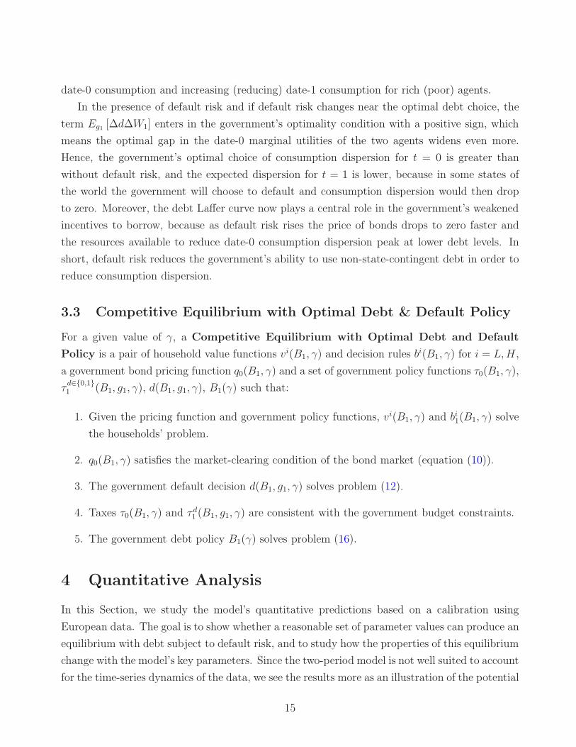
foreign investors can buy government debt. Third, a case in which proportional distortionary

taxes on consumption are used as an alternative tool for redistributive policy. Fourth, a case in

which agents have access to a second asset as vehicle for saving.

5.1 Biased Welfare Weights

Assume now that the weights of the government’s payoff function differ from the utilitarian

weights γ and 1 − γ. This can be viewed as a situation in which, for political reasons, the

government’s welfare weights are biased in favor of one group of agents. The government’s

welfare weights on L- and H-type households are denoted ω and (1 − ω) respectively, and we

refer to ω as the government’s political bias.

The government’s default decision at t = 1 is determined by the following optimization

problem:

maxd∈{0,1}

{W d=0

1 (B1, g1, γ, ω),Wd=11 (g1)

}, (18)

whereW d=01 (B1, g1, γ, ω) andW d=1

1 (g1) denote the government’s payoffs in the cases of no-default

and default respectively. Using the government budget constraints to substitute for τd=01 and

τd=11 , the government payoffs can be expressed as:

W d=01 (B1, g1, γ, ω) = ωu(y − g1 + bL1 − B1) + (1− ω)u(y − g1 + bH1 −B1) (19)

24

and

W d=11 (g1) = u(y(1− φ(g1))− g1). (20)

We can follow a similar approach as before to characterize the optimal default decision by

comparing the allocations it supports with the first-best allocations. The parameter ǫ is used

again to represent the dispersion of hypothetical decentralized consumption allocations under

repayment: cL(ǫ) = y − g1 − ǫ and cH(γ, ǫ) = y − g1 +γ

1−γǫ. Under default the consumption

allocations are again cL = cH = y(1− φ(g1))− g1. Recall that under repayment, the dispersion

of consumption across agents increases with ǫ, and under default there is zero consumption

dispersion. The repayment government payoff can now be rewritten as:

W d=0(ǫ, g1, γ, ω) = ωu(y − g1 + ǫ) + (1− ω)u

(y − g1 +

γ

1− γǫ

).

The socially efficient planner chooses its optimal consumption dispersion ǫSP as the value of ǫ

that maximizes the above expression. Since as of t = 1 the only instrument the government can

use to manage consumption dispersion relative to what the decentralized allocations support is

the default decision, it will repay only if doing so allows it to get closer to ǫSP than by defaulting.

The planner’s optimality condition is now:

u′(cH1 )

u′ (cL1 )=

u′(y − g1 +

γ

1−γǫSP)

u′ (y − g1 − ǫSP )=

(ω

γ

)(1− γ

1− ω

). (21)

This condition implies that optimal consumption dispersion for the planner is zero only if ω = γ.

For ω > γ the planner likes consumption dispersion to favor L types so that cL1 > cH1 , and the

opposite holds for ω < γ.

The key difference with political bias v. the model with a utilitarian government is that

the former can support equilibria with debt subject to default risk even without default costs.

Assuming φ(g1) = 0, there are two possible scenarios depending on the relative size of γ and ω.

First, if ω ≥ γ, the planner again always chooses default as in the setup of Section 2. This is

because for any decentralized consumption dispersion ǫ > 0, the consumption allocations feature

cH > cL, while the planner’s optimal consumption dispersion requires cH ≤ cL, and hence ǫSP

cannot be implemented. Default brings the planner the closest it can get to the payoff associated

with ǫSP and hence it is always chosen. In the second scenario ω < γ (i.e. the political bias

assigns more (less) weight to H (L) types than the fraction of each type of agents that actually

exists). In this case, the model can support equilibria with debt even without default costs. In

particular, there is a threshold consumption dispersion ǫ̂ such that default is optimal for ǫ ≥ ǫ̂,

25

where ǫ̂ is the value of ǫ at which W d=01 (ǫ, g1, γ, ω) and W d=1

1 (g1) intersect. For ǫ < ǫ̂, repayment

is preferable because W d=01 (ǫ, g1, γ, ω) > W d=0

1 (g1). Thus, without default costs, equilibria for

which repayment is optimal require two conditions: (a) that the government’s political bias

favors bond holders (ω < γ), and (b) that the debt holdings chosen by private agents do not

produce consumption dispersion in excess of ǫ̂.

Figure 6 illustrates the main quantitative predictions of the model with political bias. The

scenario with ω = γ, shown in blue corresponds to the utilitarian case of Section 4, and the other

two scenarios correspond to high and low values of ω (ωL = 0.25 and ωH = 0.45 respectively).24

Figure 6: Equilibrium of the Model with Political Bias for different values of ω

0 0.2 0.4 0.6 0.8 10

0.1

0.2

0.3

0.4

0.5



1(γ)

0 0.2 0.4 0.6 0.8 10

1

2

3

4



1(γ), γ)

ω = γ (bench.)ωL

ωH

0 0.2 0.4 0.6 0.8 10

2

4

6

8



spre

ad (%

)

0 0.2 0.4 0.6 0.8 10

0.01

0.02

0.03

0.04

0.05

0.06



1(γ), γ)

Figure 6 shows that the optimal debt level is increasing in γ. This is because the incentives

to default grow weaker and the repayment zone widens as γ increases for a fixed value of ω.

Moreover, the demand composition effect of higher γ is still present, so along with the lower

default incentives we still have the increasing per capita demand for bonds of H types. These

24Note that along the blue curve of the utilitarian case both ω and γ effectively vary together because theyare always equal to each other, while in the other two plots ω is fixed and γ varies. For this reason, the linecorresponding to the ωL case intersects the benchmark solution when γ = 0.25, and the one for ωH intersectsthe benchmark when γ = 0.45.

26

two effects combined drive the increase in the optimal debt choice of the government. It is also

interesting to note that in the ωL and ωH cases the equilibrium exists for all values of γ (even

those that are lower than ω). Without default costs each curve would be truncated exactly

where γ equals either ωL or ωH , but since these simulations retain the default costs used in the

utilitarian case, there can still be equilibria with debt for lower values of γ (as explained earlier).

In this model with political bias, the government is still aiming to optimize debt by focusing

on the resources it can reallocate across periods and agents, which are still determined by

the debt Laffer curve, and internalizing the response of bond prices to debt choices.25 This

relationship, however, behaves very differently than in the benchmark model, because now higher

optimal debt is carried at decreasing default probabilities, which leads the planner internalizing

the price response to choose higher debt, whereas in the benchmark model lower optimal debt

was carried at increasing equilibrium default probabilities, which led the planner internalizing

the price response to choose lower debt.

In the empirically relevant range of γ, and for values of ω lower than that range (since

ωL = 0.25 and ωH = 0.45, while the relevant range of γ is [0.55− 0.85]), this model can sustain

significantly higher debt ratios than the model with utilitarian payoff, and those ratios are close

to the observed European median. At the lower end of that range of γ, a government with ωH

chooses a debt ratio of about 25 percent, while a government with ωL chooses a debt ratio of

about 35 percent.

The behavior of equilibrium bond prices (panel (ii)) with either ωL = 0.25 or ωH = 0.45 differs

markedly from the utilitarian case. In particular, the prices no longer display an increasing,

convex shape, instead they are (for most values of γ) a decreasing function of γ. This occurs

because the higher supply of bonds that the government finds optimal to provide offsets the

demand composition effect that increases individual demand for bonds as γ rises. At low values

of γ the government chooses lower debt levels (panel (i)) in part because the default probability

is higher (panel (iv)), which also results in higher spreads (panel (iii)). But as γ rises and

repayment incentives strengthen (because ω becomes relatively smaller than γ), the probability

of default falls to zero, the spreads vanish, and debt levels increase. The price remains relatively

flat because, again, the higher debt supply offsets the demand composition effect.

The political bias extension yields an additional interesting result: For a sufficiently con-

centrated distribution of bond holdings (high γ), L−type agents prefer that the government

weighs the bond holders more than a utilitarian government (i.e, there are values of γ and ω

for which, comparing equilibrium payoffs under a government with political bias v. a utilitarian

25When choosing B1, the government takes into account that higher debt increases disposable income forL-type agents in the initial period but it also implies higher taxes in the second period (as long as default is notoptimal). Thus, the government is willing to take on more debt when ω is lower.

27

government, vL(B1, ω, γ) > vL(B1, γ)). To illustrate this result, Figure 7 plots the equilibrium

payoffs in the political-bias model for the two types of agents as ω varies for two values of γ

(γL = 0.15 and γH = 0.85). The payoffs for the L− and H− types are in Panels (i) and (ii),

respectively. The vertical lines identify the payoffs that would be attained with a utilitarian

government (which by construction coincide with those under political bias when ω=γ).

Figure 7: Welfare as a function of Political Bias for different values of γ

0 0.2 0.4 0.6 0.8 1

−3

−2.5

−2

−1.5

Panel (i): vL0 (γ, ω)

Welfare weights (ω)

vL0 (γL, ω)

vL0 (γH , ω)

0 0.2 0.4 0.6 0.8 1−1

−0.8

−0.6

−0.4

−0.2

0

0.2

0.4

0.6Panel (ii): vH0 (γ, ω)

Welfare weights (ω)

vH0 (γL, ω)vH0 (γH , ω)

ω = γH

ω = γL

ω = γH

ω = γL

maxmax

max

Panel (ii) shows that the payoff of H-types is monotonically decreasing in ω, because H

types always prefer the higher debt levels attained by low ω governments, since it enhances

their ability to smooth consumption at a lower risk of default. In contrast, Panel (i) shows

that the payoff of L-types is non-monotonic in ω, and has a well-defined maximum. In the

γ = γL case, the maximum point is at ω = γL, which corresponds to the equilibrium under the

utilitarian government, but when γ = γH the maximum point is at about ω = 0.75, which is

smaller than γH . Thus, in this case, ownership of public debt is sufficiently concentrated for

the agents that do not hold it to prefer a government that chooses B1 weighting the welfare

of bond holders by more than the utilitarian government. This occurs because with γH the

utilitarian government has strong incentives to default, and thus the equilibrium supports low

debt, but L−type agents would be better off if the government could sustain more debt, which

the government with ω = 0.75 can do because it weighs the welfare of bond holders more, and

thus has weaker default incentives. The L− type agents desire more debt because they are

liquidity-constrained (i.e. µL > 0) and higher debt improves the smoothing of taxation and thus

makes this constraint less tight.

28

The above results yield an important political economy implication: Under a majority voting

electoral system, in which candidates are represented by values of ω, it can be the case that

majorities of either L or H types elect governments with political bias ω < γ. This possibility is

captured in Figure 7. When the actual distribution of bond holdings is given by γH, the majority

of voters are L types, and thus it follows from Panel (i) that the government represented by the ω

at the maximum point (around 0.75) is elected. In this case, agents that do not hold government

bonds vote for a government that favors bond holders (i.e. L types are weighed at 0.75 instead

of 0.85 in the government’s payoff function). When the distribution of bond holdings is given

by γL, the majority of voters are H types and the electoral outcome is determined in Panel (ii).

Since the payoff of H types is decreasing in ω, they elect the government at the lower bound of

ω. Hence, under both γL and γH, a candidate with political bias beats the utilitarian candidate.

This result is not general, however, because we cannot rule out the possibility that there could

be a γ ≥ 0.5 such that the maximum point of the L-types payoff is where ω = γ, and hence the

utilitarian government is elected under majority voting.

5.2 International Investors

While a large fraction of sovereign debt in Europe is in hands of domestic households (for the

countries in Table 1, 60 percent is the median and 75 percent the average), the fraction in

hands of foreign investors is not negligible. For this reason, we extend the benchmark model

to incorporate foreign investors and move from a closed to an open economy. In particular,

we assume that there is a pool of international investors modeled in the same way as in the

Eaton-Gersovitz class of external default models: risk-neutral lenders with an opportunity cost

of funds equal to an exogenous, world-determined real interest rate r̄. As is common practice,

we assume that these bonds are pari passu contracts, which rules out the possibility for the

government to discriminate among borrowers when choosing to default. This also maintains the

symmetry with the baseline model, in which the government was not allowed to default on a

particular set of domestic households.

Since foreign lenders are the marginal investor of sovereign debt, in this model the price

of the bond is given by q(B1, γ) = 1−p(B1,γ)(1+r̄)

where p(B1, γ) is the default probability. More

precisely, p(B1, γ) = Eg1[d(B1, γ, g1)]. While the arbitrage condition is functionally identical to

the one of the Eaton-Gersovitz models, they embody different mechanisms. The two are similar

in indicating that, because of risk neutrality, risk premia are equal to default probabilities. But

there is a critical difference in how these probabilities are determined. In Eaton-Gersovitz models

they follow from the values of continuation v. default of a representative agent, while in our

model they are determined by comparing those values for a utilitarian social welfare function,

29

which in turn depend on the dispersion of individual payoffs of default v. repayment (and on

the welfare weights). Hence, concentration of debt ownership affects default probabilities via

changes in the relative magnitudes of individual payoffs of default v. repayment.

We let the position of foreign investors be denoted Bft , which defines also the economy’s

net foreign asset position. We assume that a fraction φf of the initial stock of debt is in their

hands.26 That is Bf0 = φfB0. A fraction (1 − φf) is distributed among domestic households

according to γ. We denote the domestic demand by Bdt = γbLt + (1 − γ)bHt . The debt market

clearing condition is

Bdt +Bf

t = Bt (22)

We do not restrict the value of [γbL1 + (1− γ)bH1 ] to be less than or equal to B1, so Bf1 could be

positive or negative. When Bf1 > 0 the country is a net external borrower, because the bonds

issued by the government are less than the domestic demand for them, and when Bf1 < 0 the

country is a net external saver.

The problems of the agents and the government remain identical to those described in Section

3. Of course, agents understand that there is a new pricing equation and that market-clearing

conditions incorporate the foreign demand. We solve the model numerically using the same

parameter values of the benchmark model. We set φf = 0.25 to match the average fraction

of foreign debt observed in our sample of European countries and r to 2 percent to match the

average real interest rate in Germany in the 2000-2007 period.

Figure 8 shows how the planner’s welfare gain of default varies with γ and B1 for different

levels of government expenditures (g1 = g1and g1 = g1). The no-equilibrium region, which

exists for the same reasons as before, is shown in dark blue. In line with the characteristics

of default incentives of the benchmark model, within the region where the equilibrium is well

defined, for a given γ, the planner’s value of default increases monotonically with the level of

debt B1. However, we observe that, contrary to the benchmark case, in the economy with

foreign lenders, conditional on B1, the welfare gain of default has an inverted-U shape in the γ

dimension. That is, for a given B1 the value of α decreases with γ for low γ, reaches a minimum

point and then increases with γ. This also determines a bell-shaped “No Equilibrium Zone.”

The intuition for this result is simple and derives from the decision rules of domestic agents (see

Figure A.12 of the Appendix for the corresponding plot). For a given level of B1, when γ is

below (γ < 0.25 for B1 = BM for example), the country is on average a foreign borrower (i.e.

Bf > 0). That implies that a default generates a direct increase in domestic resources equal to

26This assumption is made only to approximate the quantitative predictions of the model with the data butis not crucial for any of the results presented below.

30

the forgone debt payments to foreign lenders. In this region, both L−type and H−type agents

are at the borrowing limit. As γ increases, the country becomes a net saver in foreign markets.

Increases in γ are associated with an increasing portion of domestic debt in hands of H−types.

This reduces the benefit of a default on foreign lenders. However, as in the model without foreign

lenders, domestic consumption dispersion increases. For mid-range γ’s the first effect dominates

the second and repayment is the preferred option. As γ increases even further the dispersion

in domestic consumption increases to points where default is again the optimal alternative for

the government. In this region, the main driver of domestic default is redistribution among

domestic agents as in our benchmark economy.

Figure 8: Planner’s welfare gain of default α(B1, g1, γ)

Figure 9 shows the comparison of the equilibrium functions in the economy with foreign

lenders v. the benchmark economy. As we described before, the introduction of foreign lenders

and the possibility of a “foreign” default constraint debt values and result in lower debt levels

than in the benchmark, for values of γ lower than 0.75 (see Panel (i)). This is also reflected

in higher default probabilities and spreads in the economy with foreign lenders than in the

benchmark (see Panel (iii) and (iv)). By construction, the upper bound on the price of the

31

economy with foreign lenders is (1+r)−1, so the the distributive effect that negative real interest

rates have in the benchmark economy dissipate (see Panel (ii)). This induces the government to

take on more risk and redistribute via debt issuance in the economy with foreign lenders than

in the benchmark.

Figure 9: Equilibrium Domestic and Foreign Debt Holdings

0 0.2 0.4 0.6 0.8 10

0.05

0.1

0.15

0.2



1(γ)

0 0.2 0.4 0.6 0.8 10.5

1

1.5

2

2.5

3

3.5



1(γ), γ)

BenchmarkForeign Lenders

0 0.2 0.4 0.6 0.8 10

1

2

3

4

5

6

7



spre

ad (%

)

0 0.2 0.4 0.6 0.8 10

0.01

0.02

0.03

0.04

0.05

0.06



1(γ), γ)

5.3 Redistributive Taxation (Partial Default)

In the benchmark model, issuing debt in the first period and defaulting in the second are the

only tools the government can use to reduce consumption dispersion. We now examine how the

model’s predictions change by adding an alternative tool for redistribution. In particular, we

introduce a proportional consumption tax that is invariant across periods and realizations of

g1.27

27Using this tax as opposed to other taxes simplifies the solution of the model, because aggregate consumption(as a function of y and gt) is pinned down by the resource constraint, and thus known before solving the agents’problem. As a result, the algorithm does not need to iterate on the level of transfers to close the governmentbudget constraint, while introducing a wealth tax would require it. An income tax would require not onlyiterating on aggregate transfers but also extending the model to consider endogenous labor supply, because the

32

With consumption taxes, the cost of purchasing goods in the left-hand-side of the agents’

budget constraints becomes (1+ τ c)cit for i = L,H and t = 0, 1. Since aggregate consumption in

each period is still given by y − gt, the government budget constraints simplify to the following

expressions. At date 0, the constraint is:

τ0 + τ cy = g0(1 + τ c) + B0 − q0B1. (23)

In the second period, under repayment, the constraint is:

τd1=01 + τ cy = g1(1 + τ c) + B1. (24)

In the second period, under default the budget constraint is:

τd1=11 + τ cy(1− φ(g1)) = g1(1 + τ c). (25)

Using the budget constraints of agents and the government, we can proceed as with the

benchmark model and derive expressions for the difference in consumption of the two agents in

the two periods and default scenarios: cH0 − cL0 = 11−γ

[B0−q(B1,γ)B1

(1+τc)

], cH,d=0

1 − cL,d=01 = 1

1−γB1

(1+τc)

and cH,d=11 − cL,d=1

1 = 0. These expressions are similar to those presented in Section 4, except

that the terms that include public debt in the date-0 difference and the date-1 difference under

repayment are divided by (1 + τ c). Consumption taxes reduce consumption dispersion in both

instances. Intuitively, the consumption tax plays a role akin to inflation in reducing the real

value of public debt. Hence, this tax always reduces consumption dispersion in the first period

(as long as there is a primary deficit), and also always reduces dispersion in the second period

under repayment. In fact, assuming repayment, this tax is a better mechanism for redistribution

because debt can only reduce dispersion at date 0 at the expense of increasing it a date 1.

Moreover, the tax’s ability to redistribute is not hampered by the debt Laffer curve that hampers

the ability to redistribute with debt because of default risk. The tax acts in fact as a de-facto

partial default in both periods. As a result, if we allow it to be chosen optimally, letting τ c go to

infinity would be optimal because it completely removes consumption dispersion in all periods

at no cost. The purpose of this analysis, however, is to see how the existence of an alternative

redistribution tool affects the results we have obtained for debt and default risk, rather than

focus on the optimal use of the consumption tax.28

benchmark model assumes no income heterogeneity, which makes proportional income tax close to a lump-sumtax.

28The consumption tax as modeled lacks important trade-offs that would make it suboptimal to set it infinitelylarge. In particular, it is non-distortionary, because there is no labor supply choice, and because, since the tax

33

We solve the model numerically using the parameters of the benchmark calibration. For the

value of the consumption tax, we use τ c = 0.16 which is the value estimated for the Eurozone

in Mendoza, Tesar, and Zhang (2014). We also solve the model for τ c = 0.32 and τ c = 0.48,

which are two and three times larger that the data proxy.29 Figure 10 presents the comparison

of the equilibrium of the benchmark economy with the three economies with taxes. This figure

shows that the main result of the paper (the ability to support the existence of public debt with

positive default risk) is robust to incorporating distributive taxes.

Figure 10: Comparison Equilibrium Benchmark vs Proportional Consumption Taxes

0 0.2 0.4 0.6 0.8 10.04

0.06

0.08

0.1

0.12

0.14

0.16

0.18



1(γ)

0 0.2 0.4 0.6 0.8 10.5

1

1.5

2

2.5

3

3.5



1(γ), γ)

τ c = 0 (bench.)

τ c = 0.16τ c = 0.32τ c = 0.48

0 0.2 0.4 0.6 0.8 10

0.2

0.4

0.6

0.8

1

1.2

1.4



spre

ad (

%)

0 0.2 0.4 0.6 0.8 10

0.002

0.004

0.006

0.008

0.01

0.012

0.014

0.016



1(γ), γ)

As consumption taxes increase, default incentives grow weaker (see lower default probabili-

ties in Panel (iv)), which is natural because the tax reduces consumption dispersion, and hence

reduces the need for the government to use default to lower dispersion. As a result, the govern-

ment can sustain higher debt levels(see Panel (iv)), although the effect is not very large (debt

is constant, it does not distort savings decisions. The tax is also assumed to be known with perfect foresight,whereas uncertainty about inflation would have an effect similar to a partial risk of default that would affectdemand for bonds and bond prices.

29In the tax rate estimates in Mendoza, Tesar, and Zhang (2014), the highest consumption tax is observed inFinland at 24 percent.

34

increases by at most 5 percentage points for γ = 0.6 and a change in the consumption tax

from 0 to 48 percent). This effect is negligible when default incentives are weak to start with,

which occurs at low values of γ. The properties of the price function observed in the benchmark

case (i.e. increasing in γ for a given level of default risk) are sustained in the economy with

consumption taxes (see Panel (ii)). In line with the reduction in default probabilities, the model

with consumption taxes also displays lower spreads than the benchmark (see Panel (iii)).

The findings in this Section suggest that the existence of other tools for redistribution con-

tributes to support higher debt levels at lower default frequencies. The results are also interesting

as an illustration of what happens if we combine de-jure outright default with partial, de-facto

default (the latter commonly takes place via inflation, but as noted earlier the consumption tax

in this setup plays the same role as inflation in reducing the real debt burden).

5.4 A Second Asset

We review now the implications of adding a risk-free asset that agents can use as a vehicle of

savings, in addition to public debt. In particular, agents have access to a non-stochastic pro-

duction technology yit = z(kit)

θ with 0 < θ < 1, where yit is total output and kit is capital for

agent of type i in period t, respectively.30 The initial aggregate level of capital is denoted by K0.

L-type agents are now endowed with bL0 and kL0 units of public debt and capital respectively,

whileH-type agents have endowments given by bH0 =B0−γbL0(1−γ)

and kH0 =

K0−γkL0(1−γ)

. Capital depre-

ciates at rate δ. At period 0, agents choose how much of their savings they want to allocate to

public bonds bi1 ≥ 0 and capital ki1 ≥ 0.

The full characterization of the equilibrium and the detailed quantitative results are discussed

in Section A.10 of the Appendix. Here we focus only on the main results. Intuitively, the

existence of the second asset implies that agents arbitrage returns across public debt and risk-

free capital, taking into account the risk of default on public debt. In particular, the optimality

conditions for H− type agents imply:

q0

[θz(ki1)

θ−1 + 1− δ]−1 =

Eg1

[u′(ci,d=0

1 )(1− d1)]

Eg1

[u′(ci,d=0

1 )(1− d1) + u′(ci,d=11 )d1

] . (26)

Thus, the default spread of this model (i.e. the gap between the yield on government bonds and

the marginal productivity of capital) is determined by default risk, weighted by marginal utility

in each state of the world, since agents are risk-averse. From this perspective, the second asset

30The curvature in production allows us to obtain a well-defined portfolio choice of bonds and capital forprivate agents.

35

has a similar effect as introducing the foreign investor, because it introduces an opportunity

cost of funds, but with the difference that in this cost is now endogenous and falls as capital

investment rises.

Adding the second asset also affects the government’s debt and default choices. In particular,

the government now has to consider the initial distributions of both bonds and capital across

agents, and the effects of its choices on the individual capital and bond decisions {bi1, ki1},

which depend on B1 and default risk. Default is more costly, because via its effects on capital

allocations it can cause higher consumption dispersion than before.

To make this case as close as possible to the benchmark model for the quantitative analysis,

we assume ki0 = K0 (i.e. all initial heterogeneity is in initial bond holdings). Still, this results

in heterogeneous bond and capital holdings for the second period. We set z to normalize GDP

to 1, θ = 0.33 andδ = 0.10 ( standard values), and set K0 so the capital to output ratio is equal

to 2. All other parameters are the same as in the benchmark.

Agents in this setup have the option to switch from debt to capital as default risk rises, which

affects adversely the capacity of the government to issue debt. On the other hand, the weaker

default incentives because of the additional adverse consumption dispersion effects enhance the

ability to issue debt. In line with these arguments, we found that for low enough γ, so that

default is a zero-probability event, both models have nearly identical results. As γ rises up to

γ < 0.6, the model with two assets sustains higher optimal debt than the benchmark (by at

most 4 percentage points), but at higher values of γ the opposite is true (debt in the bechnmark

is at most 2 percentage points higher). Thus, optimal debt levels do not differ by wide margins,

even tough the effects of adding the second asset are noticeable.

The arbitrage condition connecting bond prices and capital returns also has interesting quan-

titative implications for spreads and bond prices. First, since reallocation of savings from debt

to capital reduces the marginal product of capital, the default risk spread rises as γ rises, and

this happens even tough the probability of default, which rises with γ, is actually lower than in

the benchmark. Second, bond prices rise at a much lower rate as γ rises than in the benchmark,

and in fact are never higher than 1 even at the highest values of γ considered (i.e. bond yields

are never negative). In this dimension, the quantitative results are very different in the setup

with two assets, although they are qualitatively similar.

6 Conclusions

This paper proposes a framework in which domestic sovereign default and public debt subject

to default risk emerge as an equilibrium outcome. In contrast with standard models of sovereign

36

default on external debt, this model highlights the role of the domestic distribution of public

debt ownership and the distributional effects of default across domestic agents in shaping the

government’s default incentives. These are features common to both the historical episodes of

outright domestic default documented by Reinhart and Rogoff (2011) and the ongoing European

debt crisis.

In this environment, the distribution of public debt across private agents interacts with the

government’s optimal default, debt issuance and tax decisions. Distributional incentives alone

cannot support equilibria with debt, because default is always optimal in the second period,

and hence the debt market cannot function in the first period. We also showed that equilibria

with debt exposed to default risk can exist if we introduce either exogenous default costs or

government preferences biased in favor of bond holders.

The main finding of the paper (i.e. that distributional incentives to default tempered by

default costs can support equilibria with debt exposed to default risk) is robust to other three

important extensions of the model: Adding foreign investors who can hold a portion of the debt

issued by the government, introducing consumption taxes as an alternative tool for redistributing

resources across agents, and adding a second asset as a vehicle for saving.

This paper is a first attempt at developing a blueprint for research into models of domestic

sovereign default driven by distributional incentives, and their interaction with agent hetero-

geneity and incomplete insurance markets. It has two main limitations, both byproducts of the

two-period life horizon: First, it takes as given a distribution of bond ownership across agents.

Second, it does not capture endogenous costs of default that would result from losing the benefits

of public debt as a vehicle for self-insurance and liquidity-provision (see Aiyagari and McGrattan

(1998))). In further work D’Erasmo and Mendoza (2014)) we are aiming to develop a framework

that takes both issues into account.

37

References

Aghion, P. and P. Bolton, 1990. “Government Domestic Debt and the Risk of Default:A Political-Economic Model of the Strategic Role of Debt.” In Public Debt Management:

Theory and History, edited by Rudiger Dornbusch and Mario Draghi. New York: Cambridge

University Press : 31544.

Aguiar, M. and M. Amador, 2013. “Fiscal Policy in Debt Constrained Economies.” NBER

Working Papers 17457.

Aguiar, M. and M. Amador, 2014. “Sovereign Debt.” Handbook of International Economics,4: 647–87.

Aguiar, M. and G. Gopinath, 2006. “Defaultable debt, interest rates and the current ac-count.” Journal of International Economics, 69(1): 64–83.

Aguiar, M., M. Amador, E. Farhi, and G. Gopinath, 2013. “Crisis and Commitment:Inflation Credibility and the Vulnerability to Sovereign Debt Crises.” NBER Working Papers

19516.

Aiyagari, R. and E. McGrattan, 1998. “The optimum quantity of debt.” Journal of Mone-

tary Economics, 42: 447–469.

Aiyagari, R., A. Marcet, T. Sargent, and J. Seppala, 2002. “Optimal Taxation withoutState-Contingent Debt.” Journal of Political Economy, 110(6): 1220–1254.

Alesina, A. and G. Tabellini, 1990. “A Positive Theory of Fiscal Deficits and GovernmentDebt.” The Review of Economic Studies, 57: 403–414.

Amador, M., 2003. “A Political Economy Model of Sovereign Debt Repayment.” Stanford

University mimeo.

Andreasen, E., G. Sandleris, and A. Van der Ghote, 2011. “The Political Economy ofSovereign Defaults.” Universidad Torcuato Di Tella, Business School Working Paper.

Arellano, C., 2008. “Default Risk and Income Fluctuations in Emerging Economies.” American

Economic Review, 98(3): 690–712.

Azzimonti, M., E. de Francisco, and V. Quadrini, 2014. “Financial Globalization, In-equality, and the Rising Public Debt.” American Economic Review, 104(8): 2267–2302.

Barro, R., 1979. “On the determination of the public debt.” Journal of Political Economy,87(5): 940–971.

Basu, S., 2009. “Sovereign debt and domestic economic fragility.” Manuscript, Massachusetts

Institute of Technology.

Bocola, L., 2014. “The Pass-Through of Sovereign Risk.” Manuscript, University of Pennsyl-

vania.

38

Boz, E., P. D’Erasmo, and B. Durdu, 2014. “Sovereign Risk and Bank Balance Sheets:The Role of Macroprudential Policies.” Manuscript.

Broner, F. and J. Ventura, 2011. “Globalization and Risk Sharing.” Review of Economic

Studies, 78(1): 49–82.

Broner, F., A. Martin, and J. Ventura, 2010. “Sovereign Risk and Secondary Markets.”American Economic Review, 100(4): 1523–55.

Brutti, 2011. “Sovereign defaults and liquidity crises.” Journal of International Economics, 84(1): 6572.

Calvo, G., 1988. “Servicing the Public Debt: The Role of Expectations.” American Economic

Review, 78(4): 647–61.

Cuadra, G., J. Sanchez, and H. Sapriza, 2010. “Fiscal Policy and Default Risk in EmergingMarkets.” Review of Economic Dynamics, 13(2): 452–469.

Davies, J., S. Sandstrm, A. Shorrocks, and E. Wolff, 2009. “The Level and Distributionof Global Household Wealth.” NBER Working Paper 15508.

Davies, J., R. Lluberas, and A. Shorrocks, 2012. “Credit Suisse Global Wealth Databook.”Zurich: Credit Suisse Reseach Institute.

D’Erasmo, P., 2011. “Government Reputation and Debt Repayment in Emerging Economies.”mimeo.

D’Erasmo, P. and E. Mendoza, 2014. “Optimal Domestic Sovereign Default.” Manuscript,

University of Pennsylvania.

Di Casola, P. and S. Sichlimiris, 2014. “Domestic and External Sovereign Debt.” Working

Paper, Stockholm School of Economics.

Dias, D., C. Richmond, and M. Wright, 2012. “In for a Penny, In for a 100 Billion Pounds:Quantifying the Welfare Benefits from Debt Relief.” mimeo.

Dixit, A. and J. Londregan, 2000. “Political Power and the Credibility of Government Debt.”Journal of Economic Theory, 94: 80105.

Dovis, A., M. Golosov, and A. Shourideh, 2014. “Sovereign Debt vs Redistributive Taxes:Financing Recoveries in Unequal and Uncommitted Economies.” mimeo.

Eaton, J. and M. Gersovitz, 1981. “Debt with Potential Repudiation: Theoretical andEmpirical Analysis.” Review of Economic Studies, 48(2): 289–309.

Ferriere, 2014. “Sovereign Default, Inequality, and Progressive Taxation.” mimeo.

Floden, M., 2001. “The effectiveness of government debt and transfers as insurance.” Journal

of Monetary Economics, 48: 81–108.

39

Gennaioli, N., A. Martin, and S. Rossi, 2014. “Sovereign default, domestic banks andfinancial institutions.” Journal of Finance.

Golosov, M. and T. Sargent, 2012. “Taxation, redistribution, and debt with aggregateshocks.” working paper Princeton University.

Guembel, A. and O. Sussman, 2009. “Sovereign Debt without Default Penalties.” Review

of Economic Studies, 76: 1297–1320.

Hall, G. and T. Sargent, 2014. “Fiscal Discrimination in Three Wars.” Journal of Monetary

Economics, 61: 148–166.

Hatchondo, J.C., L. Martinez, and H. Sapriza, 2009. “Heterogeneous Borrowers in Quan-titative Models of Sovereign Default.” International Economic Review, 50: 12951.

Heathcote, J., 2005. “Fiscal Policy with Heterogeneous Agents.” Review of Economic Studies,72: 161–188.

Jeon, K. and Z. Kabukcuoglu, 2014. “Income Inequality and Sovereign Default.” working

paper, University of Pittsburgh.

Lorenzoni, G. and I. Werning, 2013. “Slow moving debt crises.” NBER Working Paper No.

w19228.

Mendoza, E.G. and V.Z. Yue, 2012. “A General Equilibrium Model of Sovereign Defaultand Business Cycles.” Quarterly Journal of Economics, 127(2): 889–946.

Mendoza, E.G., L. Tesar, and J. Zhang, 2014. “Saving europe?: The unpleasant arith-metic of fiscal austerity in integrated economies.” National Bureau of Economic Research,

No. w20200.

Mengus, E., 2014. “Honoring Sovereign Debt or Bailing Out Domestic Residents? A Theoryof Internal Cost of Default.” WP Banque de France 480.

Panizza, U., F. Sturzenegger, and J. Zettelmeyer, 2009. “The Economics and Law ofSovereign Debt and Default.” Journal of Economic Literature, 47(3): 651–98.

Perez, D., 2015. “Sovereign Debt, Domestic Banks and the Provision of Public Liquidity.”Manuscript.

Pitchford and Wright, 2012. “Holdouts in Sovereign Debt Restructuring: A Theory of Nego-tiation in a Weak Contractual Environment.” Review of Economic Studies, 79(2): 812–837.

Pouzo, D. and I. Presno, 2014. “Optimal Taxation with Endogenous Default under Incom-plete Markets.” U.C. Berkeley, mimeo.

Reinhart, C. and K. Rogoff, 2011. “The Forgotten History of Domestic Debt.” Economic

Journal, 121, Issue 552: 319–350.

40

Sosa-Padilla, C., 2012. “Sovereign Defaults and Banking Crises.” Manuscript.

Tabellini, G., 1991. “The Politics of Intergenerational Redistribution.” Journal of Political

Economy, 99: 33557.

Tauchen, G., 1986. “Finite state Markov-chain approximation to univariate and vector autore-gressions.” Economics Letters, 20: 177–81.

Tomz and Wright, 2012. “Empirical research on sovereign debt and default.” Working Paper

Series WP-2012-06, Federal Reserve Bank of Chicago.

Vasishtha, 2010. “Domestic versus external borrowing and fiscal policy in emerging markets.”Review of International Economics, 18(5): 1058–1074.

Yue, V., 2010. “Sovereign Default and Debt Renegotiation.” Journal of International Eco-

nomics, 80 (2): 176–187.

41

Appendix

Distributional Incentives in an Equilibrium Modelof Domestic Sovereign Default

This Appendix includes additional material that provides background for some of the argu-ments made in the paper. Section A.1 provides an empirical analysis of the relationship betweendomestic debt and inequality. Section A.2 presents a deterministic version of our model withoutdefault risk and log preferences. Section A.3 extends this simplified model to incorporate ag-gregate risk. Section A.4 derives analytically the equilibrium price function for this model anddescribes its determinants. Section A.5 provides the details of the calibration exercise presentedin the paper. Section A.6 displays a set of additional figures of the benchmark model. SectionA.7 contains a sensitivity analysis of the benchmark model. Sections A.8 and A.9 introduce ad-ditional figures for the extension of the model with biased welfare weights and foreign investors,respectively. Finally, Section A.10 describes the extension of the model with two assets in detailand presents a set of figures that complement those in the main body of the paper.

A.1 Empirical Analysis Debt and Inequality

Further and more systematic empirical analysis of the relationship between wealth inequalityand public debt shows a statistically significant, bell-shaped relationship: Debt is increasingin wealth inequality when inequality is low, until the Gini coefficient reaches about 0.75, andthen becomes decreasing in wealth inequality. This finding follows from estimating a cross-country panel regression using the international database of Gini coefficients for wealth producedby Davies, Sandstrm, Shorrocks, and Wolff (2009) and Davies, Lluberas, and Shorrocks (2012),together with data on public debt-output ratios and control variables (i.e. the size of thegovernment, proxied by the ratio of government expenditures to GDP, and country fixed effects).The results of panel regressions of the debt ratio on the Gini coefficient, the square of thiscoefficient, and the controls (using the observations for 2000 and 2012) are shown in Table A.3,and Figure A.11 shows a plot of the 2012 data and the fitted regression curve. The regressionsonly explain about a tenth of the cross-country variations on debt ratios, but the linear andquadratic effects of the wealth Gini coefficient are statistically significant and opposite in sign.

42

Figure A.11: Public Debt Ratios and Wealth Inequality

Australia

Austria

Bahamas

Barbados

Belarus

Belgium

Brazil

Bulgaria

Canada Colombia

Cyprus

Czech

Denmark

Estonia

Finland

France

Georgia

Germany

Greece

Hong Kong

Hungary

Iceland

India

Indonesia

IrelandItaly

Jordan

Kazakhstan

LatviaLithuania

Luxembourg

Malaysia

Malta

Moldova

Mongolia

NetherlandsNew Zealand

NorwayPeru

Portugal

Russia

Singapore

Slovakia

Spain

Sweden

Thailand

Trinidad and Tobago

Turkey

Ukraine

United Kingdom

United States

Uruguay

0.5

11.

5B

/Y

.6 .7 .8 .9 1Wealth Gini

Note: Author’s calculations based on WDI, Davies, Sandstrm, Shorrocks, and Wolff (2009) and

Davies, Lluberas, and Shorrocks (2012). Fitted line from results presented in Table A.3

Table A.3: Panel Regressions of Public Debt Ratios and Wealth Inequality

Panel Country Fixed EffectDep. Var: Debt to GDP

Wealth Gini 17.65∗∗ 18.11∗∗

s.e. 7.06 7.22Wealth Gini2 -11.80∗∗ -12.03∗∗

s.e. 4.76 4.85G/Y - -0.010s.e. - 0.012avg. country FE -5.92∗∗ -5.95∗∗

s.e. 2.60 2.64years 2000-2012 2000-2012R2 0.118 0.136# obs. 139 139

Note: Author’s calculations based on WDI, Davies, Sandstrm, Shorrocks, and Wolff (2009) and Davies, Lluberas, and Shorrocks (2012). Debt to

GDP refers to Central Government Debt as share of GDP (source WDI). Wealth Gini as reported for each country for year 2000 and 2012 by

Davies, Sandstrm, Shorrocks, and Wolff (2009) and Davies, Lluberas, and Shorrocks (2012). G/Y corresponds to government final consumption as a

share of GDP (source WDI). Coefficients and standard errors reported are derived from a panel linear regression with Country Fixed Effects. The

sample contains 87 countries with data for years 2000 and 2012. If debt to GDP or government expenditure ratio is not available for year 2000 or 2012

data for year 1999 or 2011 is used.

43

A.2 Deterministic Model without Default Risk and Log

Utility

This part of the Appendix derives solutions for a version of the model in which low-wealth (L)types do not hold any bonds and high-wealth (H) types buy all the debt. We cover first the fullydeterministic case, without any shocks to income or government policies, and no default risk,but government expenditures may be deterministically different across periods. Governmentwants to use debt to relocate consumption across agents and across periods optimally given autilitarian welfare function. Ruling out default on initial outstanding debt, the planner tradesoff the desire to use debt to smooth taxation for L types (reduce date-0 taxes by issuing debt)against the cost of the postponement of consumption this induces on H types who save to buythe debt. In what follows, we work with cases where bL1 = 0 which might not hold dependingon the parameters of the model; however, it is a relevant benchmark since this holds for ourbaseline parameterization and all the extensions of the model we present.31 This assumptiontogether with log utility provides closed form solutions. The goal is to illustrate the mechanismsthat are driving the model when default risk and stochastic government purchases are takenout. Later in the Appendix we derive some results for the model with stochastic governmentpurchases, and make some inferences for the case with default risk.

A.2.1 Households

A fraction γ of agents are L types, and 1− γ are H types. Preferences are:

ln(ci0) + β ln(ci1) for i = L,H (A.1)

If bL1 = 0, budget constraints are:

cL0 = y − τ0, cH0 = y − τ0 + bH0 − qbH1 (A.2)

cL1 = y − τ1, cH1 = y − τ1 + bH1 (A.3)

Since L types do not save they can only consume what their budget constraints allow. This isimportant because altering taxes affects disposable income, which will in turn affect the optimaldebt choice of the government. For H types, the Euler equation is:

q = βcH0cH1

(A.4)

For L types, in order to make the assumption that they hold no assets consistent at equilibrium,it must be the case that they are credit constrained (i.e. they would want to hold negativeassets). That is, at the equilibrium price of debt their Euler equation for bonds would satisfy:

q > βcL0cL1

(A.5)

31The L− type agents will be credit constrained (i.e. bL1 = 0) the lower bL0 , B0 and B1.

44

A.2.2 Government

The government budget constraints are:

τ0 = g0 +B0 − qB1 (A.6)

τ1 = g1 +B1 (A.7)

The initial debt B0 ≥ 0 is taken as given and the government is assumed to be committed torepay it.

The social planner seeks to maximize this utilitarian social welfare function:

γ(ln(cL0 ) + β ln(cL1 )) + (1− γ)(ln(cH0 ) + β ln(cH1 )) (A.8)

A.2.3 Competitive equilibrium in the bond market

A competitive equilibrium in the bond market for a given supply of government debt B1 is givenby a price q that satisfies the market-clearing condition of the bond market: γbL1+(1−γ)bH1 = B1.By construction the same condition is assumed to hold for the initial conditions bH0 and B0. SincebL0 = 0, this implies that the initial wealth of H-types is given by bH0 = B0/(1− γ).

Rewriting the Euler equation of H types using the budget constraint, the government budgetconstraints and the bond market-clearing conditions when bL1 = 0 yields:

q = βy − g0 +

(γ

1−γ

)B0 − q

(γ

1−γ

)B1

y − g1 +(

γ

1−γ

)B1

(A.9)

Hence, the equilibrium price of bonds for a given government supply is:

q(B1) = βy − g0 +

(γ

1−γ

)B0

y − g1 +(

γ

1−γ

)(1 + β)B1

(A.10)

Note that this price is not restricted to be lower than 1 (i.e. q(B1) > 1 which implies anegative real rate of return on government debt can be an equilibrium outcome). In particular,as γ rises the per capita bond demand of H-types increases and this puts upward pressure onbond prices, and even more so if the government finds it optimal to offer less debt than theinitial debt, as we showed numerically and explain further below. As γ → 1, the limit of theequilibrium price goes to q(B1) =

β

1+βB0

B1even tough market-clearing requires the demand of the

infinitesimal small H type to rise to infinity.After some simplification, the derivative of this price is given by:

q′(B1) =−q(B1)

(γ

1−γ

)(1 + β)

[y − g1 +

(γ

1−γ

)(1 + β)B1

] (A.11)

45

which at any equilibrium with a positive bond price satisfies q′(B1) < 0 (notice cH1 > 0 impliesthat the denominator of this expression must be positive).

Consider now what happens to this equilibrium as the fraction of L-types vanishes. Asγ → 0, the economy converges to a case where there is only an H type representative agent,and the price is simply q(B1) = β y−g0

y−g1, which is in fact independent of B1 and reduces to β if

government purchases are stationary. Trivially, in this case the planner solves the same problemas the representative agent and the equilibrium is efficient. Also, for an exogenously given B0

and stationary g, the competitive equilibrium is stationary at this consumption level:

cH = y − g +

(γ

1− γ

)B0

1 + β(A.12)

and the optimal debt is:

B1 =B0

1 + β(A.13)

Hence, in this case consumption and disposable income each period are fully stationary, yet theoptimal debt policy is always to reduce the initial debt by the fraction 1/(1 + β). This is onlybecause of the two-period nature of the model. With an infinite horizon, the same bond pricewould imply that an equilibrium with stationary consumption and an optimal policy that issimply B1 = B0. It also follows trivially that carrying no initial debt to start with would befirst-best, using lump-sum taxation to pay for g.

A.2.4 Optimal debt choice

The government’s optimal choice of B1 in the first period solves this maximization problem:

maxB1

{γ [ln (y − g0 − B0 + q(B1)B1) + β ln (y − g1 − B1)]

+(1− γ)[ln(y − g0 +

(γ

1−γ

)B0 − q(B1)

(γ

1−γ

)B1

)+ β ln(y − g1 +

(γ

1−γ

)B1)]}

(A.14)

where q(B1) = βy−g0+( γ

1−γ )B0

y−g1+( γ

1−γ )(1+β)B1.

The first-order condition is:

γ[u′(cL0 ) [q

′(B1)B1 + q(B1)]− βu′(cL1 )]

(A.15)

+(1− γ)

(γ

1− γ

)[−u′(cH0 ) [q

′(B1)B1 + q(B1)] + βu′(cH1 )]= 0

Using the Euler equation of the H types and simplifying:

u′(cL0 ) +

[u′(cL0 )q(B1)− βu′(cL1 )

q′(B1)B1

]= u′(cH0 ) (A.16)

This expression is important, because it defines a wedge between equating the two agents’marginal utility of consumption that the planner finds optimal to maintain, given that the onlyinstrument that it has to reallocate consumption across agents is the debt. Notice that, since as

46

noted earlier for L types to find it optimal to hold zero assets it must be that they are ”creditconstrained,” their Euler equation implies that at the equilibrium price: u′(cL0 )q(B1)−βu′(cL1 ) >0. Hence, the above optimality condition for the planner together with this condition imply thatthe optimal debt choice supports u′(cL0 ) > u′(cH0 ) or c

H0 > cL0 , and notice that from the budget

constraints this also implies B0 − q(B1)B1 > 0, which implies B1/B0 < 1/q(B1). Furthermore,the latter implies that the optimal debt must be lower than any initial B0 for any q(B1) ≥ 1,and also for ”sufficiently high” q(B1).

Comparison with no-debt equilibrium: Notice that since B0−q(B1)B1 > 0, the planneris allocating less utility to L type agents than those agents would attain without any debt.Without debt, and a tax policy τt = gt, all agents consume y − gt every period, but with debtL-types consume less each period given that B1 > 0 and B0 − q(B1)B1 > 0. Compared withthese allocations, when the planner finds optimal to choose B1 > 0 is because he is trading offthe pain of imposing higher taxes in both periods, which hurts L types, against the benefit theH types get of having the ability to smooth using government bonds. Also, B0 − q(B1)B1 > 0highlights that there is a nontrivial role to the value of B0, because if B0 were zero B1 wouldneed to be negative which is not possible by construction. Hence, the model only has a sensiblesolution if there is already enough outstanding debt (and wealth owned by H type agents) thatgives the government room to be able to improve the H type’s ability to smooth across the twoperiods, which they desire to do more the higher is B0.

Comparison with sub-optimal debt equilibrium: By choosing positive debt, the gov-ernment provides tax smoothing for L types. Given B0 and the fact that B0 − q(B1)B1 > 0,positive debt allows to lower date-0 taxes, which increases consumption of L types (sincecL0 = y − g0 − B0 + q(B1)B1). The same policy lowers the consumption of H types (since

cH0 = y − g0 +(

γ

1−γ

)(B0 − q(B1)B1)). Hence, debt serves to redistribute consumption across

the two agents within the period. This also changes inter-temporal consumption allocations,with the debt reducing L types consumption in the second period and increasing H types con-sumption. Hence, with commitment to repay B0, the debt will be chosen optimally to tradeoff these social costs and benefits of issuing debt to reallocate consumption atemporally acrossagents and intertemporally.

It is also useful to notice that the demand elasticity of bonds is given by η ≡ q(B1)/ (q′(B1)B1) ,

so the marginal utility wedge can be expressed as η[u′(cL0 )−

βu′(cL1 )

q(B1)

]and the planner’s optimal-

ity condition reduces to:

1 + η

[1−

βu′(cL1 )

q(B1)u′(cL0 )

]=

u′(cH0 )

u′(cL0 )(A.17)

Hence, the planner’s marginal utility wedge is the product of the demand elasticity of bonds and

the L-type agents shadow value of being credit constrained (the difference 1 −βu′(cL1 )

q(B1)u′(cL0 )> 0,

which can be interpreted as an effective real interest rate faced by L-type agents that is higherthan the return on bonds). The planner wants to use positive debt to support an optimalwedge in marginal utilities only when the demand for bonds is elastic AND L-type agents areconstrained.

47

A.3 Extension to Include Government Expenditure Shocks

Now consider the same model but government expenditures are stochastic. In particular, real-izations of government purchases in the second period are given by the set [g11 < g21 < ... < gM1 ]

with transition probabilities denoted by π(gi1|g0) for i = 1, ...,M withM∑i=1

π(gi1|g0) = 1.

A.3.1 Households

Preferences are now:

ln(ci0) + β

(M∑

i=1

π(gi1|g0) ln(ci1)

)for i = L,H (A.18)

Budget constraints are unchanged:

cL0 = y − τ0, cH0 = y − τ0 + bH0 − qbH1 (A.19)

cL1 = y − τ1, cH1 = y − τ1 + bH1 (A.20)

We still analyze cases where L types do not save, so they only consume what their budgetconstraints allow. For H types, the Euler equation becomes:

q = βM∑

i=1

π(gi1|g0)

(cH0cH1

)(A.21)

For L types, in order to make the assumption that they hold no assets consistent at equilibrium,their Euler equation for bonds must satisfy:

q > βM∑

i=1

π(gi1|g0)

(cL0cL1

)(A.22)

A.3.2 Government

The government budget constraints are unchanged:

τ0 = g0 +B0 − qB1

τ1 = g1 +B1

The initial debt B0 ≥ 0 is taken as given and the government is assumed to be committed torepay it.

The social planner seeks to maximize this utilitarian social welfare function:

γ

(ln(cL0 ) + β

M∑

i=1

π(gi1|g0) ln(cL1 )

)+ (1− γ)

(ln(cH0 ) + β

M∑

i=1

π(gi1|g0) ln(cH1 )

)(A.23)

48

A.3.3 Competitive equilibrium in the bond market

A competitive equilibrium in the bond market for a given supply of government debt B1 is givenby a price q that satisfies the market-clearing condition of the bond market: bH1 = B1/(1− γ).When bL1 = 0 the equilibrium price can be derived from the H-types Euler equation.

We can solve the model in the same steps as before. First, rewrite the Euler equation of Htypes using their budget constraints, the government budget constraints and the market-clearingconditions:

q = β

M∑

i=1

π(gi1|g0)

y − g0 +

(γ

1−γ

)B0 − q

(γ

1−γ

)B1

y − g1 +(

γ

1−γ

)B1

(A.24)

From here, we can solve again for the equilibrium price at a given supply of bonds:

q(B1) = β

(y − g0 +

(γ

1−γ

)B0

)(M∑i=1

π(gi1|g0)

y−g1+( γ

1−γ )B1

)

1 +(

γ

1−γ

)βB1

(M∑i=1

π(gi1|g0)

y−g1+( γ

1−γ )B1

) (A.25)

As γ → 0 we converge again to the world where there is only an H type representative agent, butnow the pricing formula reduces to the standard formula for the pricing of a non-state-contingent

asset q(B1) = β

(M∑i=1

π(gi1|g0)y−g0y−g1

). As γ → 1 the equilibrium degenerates again into a situation

where market clearing requires the demand of the infinitesimal small H type to rise to infinity.The derivative of the price at any equilibrium with a positive bond price satisfies q′(B1) < 0.

To show this, define Π(B1) ≡M∑i=1

π(gi1|g0)

y−gi1+(γ

1−γ )B1which yields Π′(B1) = −

M∑i=1

π(gi1|g0)(γ

1−γ )

(y−gi1+(γ

1−γ )B1)2 < 0.

Then taking the derivative q′(B1) and simplifying we get:

q′(B1) =β(y − g0 +

(γ

1−γ

)B0

) [Π′(B1)− β

(γ

1−γ

)(Π(B1))

2]

(1 + β

(γ

1−γ

)B1Π(B1)

)2 (A.26)

Since Π′(B1) < 0 and positive cH0 implies y − g0 +(

γ

1−γ

)B0 > 0, it follows that q′(B1) < 0.

We can also gain some insight into the implicit risk premium (the ratio q(B1)/β)) and therelated question of why the asset price can exceed 1 in this setup. Recall that in fact thelatter was already possible without uncertainty when γ is large enough, because of the demandcomposition effect (higher γ implies by market clearing that the fewer H type agents need todemand more bonds per capita, so the bond price is increasing in γ and can exceed 1). Theissue now is that, as numerical experiments show, an increase in the variance of g1 also results inhigher bond prices, and higher than in the absence of uncertainty, and again for γ large enoughwe get both q(B1) > 1 and q(B1)/β > 1. The reason bond prices increase with the variabilityof government purchases is precautionary savings. Government bonds are the only vehicle of

49

saving, and the incentive for this gets stronger the larger the variability of g1. Hence, the priceof bonds is higher in this stochastic model than in the analogous deterministic model becauseof precautionary demand for bonds, which adds to the effect of demand composition (i.e. theprice is higher with uncertainty than without at a given γ).

A.3.4 Optimal debt choice

The government’s optimal choice of B1 solves again a standard maximization problem:

maxB1

γ

[ln (y − g0 −B0 + q(B1)B1) + β

M∑i=1

π(gi1|g0) ln (y − g1 − B1)

]

+(1− γ)

[ln(y − g0 +

(γ

1−γ

)B0 − q(B1)

(γ

1−γ

)B1

)

+βM∑i=1

π(gi1|g0) ln(y − g1 +(

γ

1−γ

)B1)

]

(A.27)

where q(B1) is given by the expression solved for in the competitive equilibrium.The first-order condition is:

γ

[u′(cL0 ) [q

′(B1)B1 + q(B1)]− β

M∑

i=1

π(gi1|g0)u′(cL1 )

](A.28)

+(1− γ)

(γ

1− γ

)[−u′(cH0 ) [q

′(B1)B1 + q(B1)] + βM∑

i=1

π(gi1|g0)u′(cH1 )

]= 0

Using the stochastic Euler equation of the H types and simplifying:

u′(cL0 ) [q′(B1)B1 + q(B1)]− β

M∑

i=1

π(gi1|g0)u′(cL1 ) = u′(cH0 )q

′(B1)B1 (A.29)

u′(cL0 ) +

u′(cL0 )q(B1)− β

M∑i=1

π(gi1|g0)u′(cL1 )

q′(B1)B1

= u′(cH0 ) (A.30)

This last expression, compared with the similar expression of the planner without uncertainty,implies that in the planner’s view, the government expenditure shocks only matter to the ex-tent that they affect the shadow price of the binding credit constraint of the L types. Asbefore, since for L types to find it optimal to hold zero assets it must be that they are ”creditconstrained,” their Euler equation would imply that at the equilibrium price: u′(cL0 )q(B1) −

βM∑i=1

π(gi1|g0)u′(cL1 ) > 0. Hence, the above optimality condition for the planner together with

this condition imply that the optimal debt choice supports u′(cL0 ) > u′(cH0 ) or cH0 > cL0 , andnotice that from the budget constraints this implies again B0 − q(B1)B1 > 0, which implies

50

B1/B0 < 1/q(B1). Furthermore, the latter implies that the optimal debt must be lower thanany initial B0 for any q(B1) ≥ 1, and also for ”sufficiently high” q(B1). Thus the optimal debtchoice again has an incentive to be lower than the initial debt.

A.4 Pricing Function: Stochastic Model with Default

We can also make an inference about what the pricing function looks like in the model withdefault risk, because with default we have a similar Euler equation, except that the summationthat defines the term Π(B1) above will exclude all the states of g1 for which the governmentchooses to default on a given B1 (and also at a given value of γ). That is, the term in question

becomes ΠD(B1) ≡M∑

{i:d(B1,gi1,γ)=0}

π(gi1|g0)

y−gi1+(γ

1−γ )B1≤ Π(B1), and the pricing function with default

risk is:

qD(B1) = β

(y − g0 +

(γ

1−γ

)B0

)ΠD(B1)

1 +(

γ

1−γ

)βB1ΠD(B1)

≤ q(B1) (A.31)

Moreover, it follows from the previous analysis that this pricing function is also decreasing

in B1 (qD′(B1) < 0), and ΠD′(B1) = −M∑

{i:d(B1,gi1,γ)=0}

π(gi1|g0)(γ

1−γ )

(y−gi1+(γ

1−γ )B1)2 is negative but such that

Π′(B1) ≤ ΠD′(B1) < 0. Also, it is clear from the above pricing functions that if the probabilityof default is small, so that are only a few values of i for which d(B1, g

i1, γ) = 1 and/or the

associated probability π(gi1|g0) is very low, the default pricing function will be very similar tothe no-default pricing function.

If we define the default risk spread as S(B1, γ) ≡ [1/qD(B1, γ)] − [1/q(B1, γ)], where γ hasbeen added as an argument of the price functions because those prices also depend on variationsin inequality, the spread reduces to the following expression:

S(B1, γ) =

1

β(y − g0 +

(γ

1−γ

)B0

)

[

1

ΠD(B1, γ)−

1

Π(B1, γ)

]

Clearly since ΠD(B1, γ) ≤ Π(B1, γ) the spread is non-negative, and it is strictly positive if thereis default at equilibrium. The spread is increasing in B1, because as the debt rises default ischosen optimally in more of the possible realizations of gi1 and hence ΠD(B1, γ) falls furtherbelow Π(B1, γ), so that the gap between the reciprocals of these two terms widens. Note alsothat the spread is a multiple of the gap between these reciprocals, with the multiple given by

1/β(y − g0 +

(γ

1−γ

)B0

). As a result, the total date-0 resources available for consumption of

the H-types (y−g0+(

γ

1−γ

)B0) have a first-order negative effect on the spreads. This is because,

as this measure of income rises, the marginal utility of date-0 consumption of H types falls, whichpushes up bond prices. The are also second order effects, because the equilibrium allocation ofB1 also depends on that income measure, and thus ΠD(B1, γ) and Π(B1, γ) vary with it as well,

51

but these are not considered here.In terms of the effect of changes in γ on S, notice that there are two effects. First, there is

a negative effect because higher γ means that, for a given B0, the resources available for date-0 consumption of H types increase, since fewer H type agents need to demand enough initialbonds to clear the bond market, which means that per-capita each of the H types hold moredate-0 bonds and have more bond income. Second, there is a positive effect because rising γweakens default incentives as the welfare of the wealthy is valued more, and hence default isoptimally chosen in more states, which increases

[1/ΠD(B1, γ)− 1/Π(B1, γ)

]. Thus, in principle

the response of the spread to increases in inequality is ambiguous. The weaker the response ofthe default probability to changes in γ, however, the more likely it is that the first effect willdominate and the spreads will be a decreasing function of inequality.

A.5 Calibration of the Benchmark Model

The model is calibrated to annual frequency, and most of the parameter values are set so as toapproximate some of the model’s predicted moments to those observed in the European data.The preference parameters are set to standard values: β = 0.96, σ = 1. We also assume forsimplicity that L types start with zero wealth, bL0 = 0.32 We assume that

ln(g1) ∼ N

((1− ρg) ln(µg) + ρg ln(g0),

σ2e

(1− ρ2g)

).33

The parameters of this process are pinned down by estimating an AR(1) model with 1995-2012data of the government expenditures-GDP ratio (in logs) for France, Germany, Greece, Ireland,Italy, Spain and Portugal. Given the parameter estimates for each country, we set µg, ρg andσe to the corresponding cross-country average. This results in the following values µg = 0.1812,ρg = 0.8802 and σe = 0.017. Given these moments, we set g0 = µg and use Tauchen (1986)quadrature method with 45 nodes inG1 ≡ {g

1, . . . , g1} to generate the realizations and transition

probabilities of the Markov process that drives expectations about g1.34

We abstain from setting a calibrated value for γ and instead show results for γ ∈ [0, 1]. Note,however, that data for the United States and Europe suggest that the empirically relevant rangefor γ is [0.55, 0.85], and hence when taking a stance on a particular value of γ is useful we useγ = 0.7, which is the mid point of the plausible range.35

32σ = 1 and bL0 = 0 are also useful because, as we show in the Appendix, under these assumptions we canobtain closed-form solutions and establish some results analytically.

33This specification allows us to control the correlation between g0 and g1 via ρg, the mean of the shock via

µg and the variance of the unpredicted portion via σ2e . Note that if g0 = µg, ln(g1) ∼ N(ln(µg),

σ2

g

(1−ρ2e)).

34As it is standard, we assume that g1 is an equally spaced grid with log(g1) and log(g1) located -/+ 3 standard

deviations from log(µg) respectively.35In the United States, the 2010 Survey of Consumer Finances indicates that only 12% of households hold

savings bonds but 50.4% have retirement accounts (which are very likely to own government bonds). Thesefigures would suggest values of γ ranging from 50% to 88%. In Europe, comparable statistics are not availablefor several countries, but recent studies show that the wealth distribution is highly concentrated and that thewealth Gini coefficient ranges between 0.55 and 0.85 depending on the country and the year of the study (see

52

Average income y is calibrated such that the model’s aggregate resource constraint is consis-tent with the data when GDP is normalized to one. This implies that the value of households’aggregate endowment must equal GDP net of fixed capital investment and net exports, sincethe latter two are not explicitly modeled. The average for the period 1970-2012 for the sameset of countries used to estimate the g1 process implies y = 0.7883. Note also that under thiscalibration of y and the Markov process of g1, the gap y−g1 is always positive, even for g1 = g1,which in turn guarantees cH1 > 0 in all repayment states.

We set the value of B0 to match the median value of government debt for Euro-zone countriesreported in Table 1 of the paper. As we describe in the next section, even though the optimal B1

(close to 15 percent of GDP for γ ∈ [0.55, 0.85]) is higher than those observed in the sovereigndebt literature, in this two-period model the consumption smoothing mechanism induces areduction in the optimal B1 relative to the initial condition B0 even in a deterministic version ofthe model with stationary government purchases. Under these assumptions, the optimal debtchoice is decreasing in γ and has an upper bound of B1 = B0/(1 + β) as γ → 0.36 In addition,when default risk is introduced debt needs to be below the level that would lead the governmentto default in the second period with probability 1, and above the level at which either cL0 or cH1become non-positive, otherwise there is no equilibrium.

The functional form of the default cost function is the following: φ(g1) = φ0 + (g1 − g1)/y,where g1 is calibrated to represent an “unusually large” realization of g1 set equal to the largestrealization in the Markov process of government expenditures, which is in turn set equal to3 standard deviations from the mean (in the process in logs).37 We calibrate φ0 to matchan estimate of the observed frequency of domestic defaults. According to Reinhart and Rogoff(2011), historically, domestic defaults are about 1/4 as frequent as external defaults (68 domesticv. 250 external in data since 1750). Since the probability of an external default has beenestimated in the range of 3 to 5% (see for example Arellano (2008)), we estimate the probabilityof a domestic default at about 1%. The model is close to this default frequency on average whensolved over the empirically relevant range of γ′s (γ ∈ [0.55, 0.85]) if we set φ0 = 0.004. Note,however, that this calibration of φ0 to target the default probability and the calibration of B0 tothe target described early needs to be done jointly by repeatedly solving the model until bothtargets are well approximated.

Davies, Sandstrm, Shorrocks, and Wolff (2009)). In our model, if bL0 = 0, the Gini coefficient of wealth is equalto γ.

36This occurs because as γ → 0, the model in deterministic form collapses to a representative agent economyinhabited by H types where the optimal debt choice yields stationary consumption, q0 = 1/β, and B1 = B0/(1+β). In contrast, an infinite horizon, stationary economy yields B1 = B0 (see Appendix for details).

37This cost function shares a key feature of the default cost functions widely used in the external defaultliterature to align default incentives so as to support higher debt ratios and trigger default during recessions (seeArellano (2008) and Mendoza and Yue (2012)): The default cost is an increasing function of disposable income(y − g1). In addition, this formulation ensures that households’ consumption during a default never goes abovea given threshold.

53

A.6 Additional Figures: Benchmark Model

Figure A.12 shows two panels with the optimal default decision for different values of g1. Theplots separate the regions where the government chooses to repay (d(B1, g1, γ) = 0 shown inwhite), where it chooses to default (d(B1, g1, γ) = 1 in green) and where the equilibrium doesnot exist (in blue).

Figure A.12: Government default decision d(B1, g1, γ)

The repayment region (d(B1, g1, γ) = 0) corresponds to the region with α(B1, g1, γ) < 0.Hence, the government defaults at higher B1 the lower a given γ, or at higher γ the lowera given B1. Moreover, the two plots show that when g1 = g1 the government defaults forcombinations of γ and B1 for which it repays when g1 = g

1. Thus, default occurs over a wider

set of (B1, γ) pairs at higher levels of government expenditures, and thus it is also more likelyto occur.

We examine further the behavior of the default decision by computing the threshold value ofγ such that the government is indifferent between defaulting and repaying in period for a given(B1, g1). These indifference thresholds (γ̂(B1, g1)) are plotted in Figure A.13 against debt levelsranging from 0 to 0.4 for three values of government expenditures {g1, µg, g1}. For any given(B1, g1), the government chooses to default if γ ≥ γ̂.

54

Figure A.13: Default Threshold γ̂(B1, g1)

0 0.05 0.1 0.15 0.2 0.25 0.3 0.350

0.1

0.2

0.3

0.4

0.5

0.6

0.7

0.8

0.9

1

Gov. Debt (B1)

Defau

ltThresho

ld(γ̂)

γ̂(B1, g)

γ̂(B1, µg)γ̂(B1, g)

Figure A.13 shows that the default threshold is decreasing in B1. Hence, the governmenttolerates higher debt ratios without defaulting only if wealth concentration is sufficiently low.Also, default thresholds are decreasing in g1, because the government has stronger incentivesto default when government expenditures are higher (i.e. the threshold curves shift inward).38

This last feature of γ̂ is very important to determine equilibria with debt subject to default risk.If, for a given value of B1, γ is higher than the curve representing γ̂ for the lowest realization inthe Markov process of g1 (which is also the value of g1), the government defaults for sure and,as explained earlier, there is no equilibrium. Alternatively, if for a given value of B1, γ is lowerthan the curve representing γ̂ for the highest realization of g1 (which is the value of g1), thegovernment repays for sure and debt would be issued effectively without default risk. Thus, forthe model to support equilibria with debt subject to default risk, the optimal debt chosen bythe government in the first period for a given γ must lie between these two extreme thresholdcurves. We show that this is the case later in this Section. Figure A.14 shows intensity plots ofthe equilibrium tax functions.

38γ̂ approaches zero for B1 sufficiently large, but in Figure A.13 B1 reaches 0.40 only for exposition purposes.

55

Figure A.14: Equilibrium Tax Functions τd(B1,g1,γ)1

Putting together these plots with those of the default decision in Figure A.12 illustrates themodel’s distributional incentives to default from the perspective of tax policy. If the governmentdefaults, the tax is τ1 = g1, but if it repays the tax is τ1 = g1 + B1. Since all agents pay thesame taxes but L types do not collect bond repayments, the lower taxes under default provide adistributional incentive to default that is larger when wealth is more concentrated. Figure A.14shows that, for given g1, the repayment scenarios with higher taxes are more likely when a largefraction of households hold debt (low γ) and thus benefit from a repayment, or when the debtis low so that the distributional incentives to default are weak. Moreover, equilibria with highertaxes are more likely to be observed at low than at high levels of government expenditures,because default is far likely with the latter.

Figure A.15 plots the bond demand decision rules (for given B1) of the H types in the samelayout as the bond prices (i.e. as functions of γ for three values of B1).

39 This plot validatesthe intuition provided above about the properties of these agents’ bond demand function. Inparticular, as γ increases, the demand for bonds ofH types grows at an increasing rate, reflectingthe combined effects of higher per-capita demand by a smaller fraction of H-type agents and arising default risk premium. Thus, the convexity of these bond decision rules reflects the effectsof wealth dispersion on demand composition and default risk explained earlier.

39We do not include the bond decision rules for L types because they are credit constrained (i.e. their Eulercondition holds with inequality) and choose bL1 = bL0 = 0.

56

Figure A.15: Equilibrium HH bond decision rules bi1

0.2 0.3 0.4 0.5 0.6 0.7 0.8 0.90

0.5

1

1.5


bH1 (B1,L, γ)

bH1 (B1,M , γ)

bH1 (B1,H , γ)

Figure A.16 shows the debt Laffer curves for five values of γ in the [0.05,0.95] range.40

40Each curve is truncated at values of B1 in the horizontal axis that are either low enough for cL0 ≤ 0 orhigh enough for default to be chosen for all realizations of g1, because as noted before in these cases there is noequilibrium.

57

Figure A.16: Debt Laffer Curve

0 0.05 0.1 0.15 0.2 0.25 0.3 0.35 0.40

0.05

0.1

0.15

0.2

0.25

0.3

0.35”Laffer” Curve B1 ∗ q(B1, γ)

Government Debt (B1)

B1∗q(B

1,γ)

B1 ∗ q(B1, γ = 0.05)B1 ∗ q(B1, γ = 0.25)B1 ∗ q(B1, γ = 0.50)B1 ∗ q(B1, γ = 0.75)B1 ∗ q(B1, γ = 0.95)Bx

1

When γ ≥ 0.50, B∗1(γ) is located at the maximum of the corresponding Laffer curve. In these

cases, setting debt higher than at the maximum of the Laffer curve is suboptimal because defaultrisk reduces bond prices sharply, moving the government to the downward sloping region of theLaffer curve, and setting it lower is also suboptimal because then default risk is low and extraborrowing generates more resources since bond prices change little, leaving the government in theupward sloping region of the Laffer curve. Thus, if the optimal debt has a nontrivial probabilityof default, the government’s debt choice exhausts its ability to raise resources by borrowing.

A.7 Sensitivity Analysis: Benchmark Model

This Section presents the results of a set of counterfactuals that shed more light on the workingsof the model and also show some results for the case in which the social welfare function hasbiased weights that do not correspond to the fractions of L and H types in the economy. Thesensitivity analysis studies how the main results are affected by changes in the initial debt B0,initial government expenditures g0, and the constant in the default cost function φ0.

A.7.1 Lower Initial Debt Level B0

Figure A.17 compares the optimal government debt and associated equilibrium bond prices,spreads and default probability under the original calibration with B0 = 0.35 and a value thatis 20% lower (B0,L = 0.28).

58

Panel (i) shows that the optimal debt choice is always lower for the lower B0, but thedifference narrows as γ rises. This occurs because at low γ default risk plays a negligible role,and the demand composition effect implies lower per-capita demand for bonds from H typeagents and a smaller fraction of credit-constrained L types, so the government wants to sell lessdebt. But once default risk becomes relevant, the optimal debt choice is about the same.

With the lower B0, bond prices are uniformly lower albeit slightly (panel (ii)), spreads areincreasing as γ rises for a wider range of γ and attain a lower maximum (panel (iii)), andthe same is true for default probabilities (panel (iv)). Bond prices are lower with lower initialdebt because for a given γ this implies lower initial wealth of H types (bH0 ), and in turn thisrequires a lower bond price to clear the market. This effect is stronger than two other effects thatpush bond prices in the opposite direction: First, the slightly lower debt B1 that the governmentfinds optimal to supply at lower levels of B0. Second, the higher disposable income of householdsresulting from the lower date-0 taxes needed to repay lower levels of B0, which increases demandfor bonds.

Figure A.17: Changes in Initial Government Debt B0

0 0.5 10

0.05

0.1

0.15

0.2

0.25



1(γ)

B0 (bench.)B0,L

0 0.5 10.5

1

1.5

2

2.5

3

3.5



1(γ), γ)

0 0.5 10

0.2

0.4

0.6

0.8

1

1.2

1.4



spre

ad (%

)

0 0.5 10

0.005

0.01

0.015

0.02



1(γ), γ)

59

In terms of the implications for the empirically relevant range of γ in the European data,these results show that at the lower B0 the model continues to predict debt ratios of about 8 to12%, but now at spreads that are only half (40 v. 100 basis points) and at default probabilitiesbelow 1 percent instead of 1 to 1.5 percent. Moreover, these results also show that spreads anddefault probabilities can display richer patterns than the ones found in the initial calibration.

A.7.2 Lower Initial Government Expenditures g0

Figure A.18 compares the model’s equilibrium outcomes under the calibrated value of initialgovernment expenditures, g0 = µg = 0.181, and a scenario in which g0 is 1.5 standard deviationsbelow the mean, g0,L = 0.171.

Figure A.18: Changes in Initial Government Expenditures g0

0 0.5 10

0.05

0.1

0.15

0.2



1(γ)

0 0.5 10.5

1

1.5

2

2.5

3

3.5



1(γ), γ)

g0 = µg (bench.)

g0,L

0 0.5 10

0.5

1

1.5



spre

ad (%

)

0 0.5 10

0.005

0.01

0.015

0.02



1(γ), γ)

Like the reduction in B0, the reduction in g0 increases date-0 disposable income via lowerdate-0 taxes. They differ, however, in two key respects: First, changes in g0 affect the expectedlevel of government expenditures for t = 1, as reflected in changes in the transition probabilitieswhich are conditional on g0. Second, changes in g0 do not affect the aggregate wealth of theeconomy and the initial bond holdings of H types.

Panel (i) shows that the optimally debt is slightly higher with lower g0, unless γ is below0.35. This reflects the fact that the lower g0 allows the government to issue more debt in theinitial period, because the likelihood of hitting states with sufficiently high g1 for optimal defaultto occur in the second period is lower. This also explains why in panels (ii)-(iv), despite thehigher optimal debt with the lower g0, bond prices, default probabilities and spreads are lower.

60

Moreover, optimal debt is about the same with lower g0 as in the initial calibration for γ ≤ 0.35because at this low level of wealth concentration default risk is not an issue and the mechanismthat we just described is irrelevant.

A.7.3 Fixed Cost of Default φ0

Panels (i)− (iv) in Figure A.19 compare the equilibrium outcomes for the initial calibration ofthe default cost parameter (φ0 = 0.004) with an scenario with a higher values (φ0,H = 0.02).

Figure A.19: Changes in Cost of Default φ0

0 0.5 10

0.05

0.1

0.15

0.2



1(γ)

0 0.5 10.5

1

1.5

2

2.5

3

3.5



1(γ), γ)

φ0 (bench.)

φ0,H

0 0.5 10

0.5

1

1.5



spre

ad (%

)

0 0.5 10

0.005

0.01

0.015

0.02



1(γ), γ)

Qualitatively, the changes in the equilibrium are in the direction that would be expected.Higher default costs increase the optimal debt and reduce bond prices, spreads and defaultprobabilities. Quantitatively, however, the changes in optimal debt and bond prices are small,while the reduction in spreads and default probabilities are significantly larger.

A.8 Additional Figures: Model with BiasedWelfareWeights

Adding default costs to the political bias setup (φ(g1) > 0) makes it possible to support repay-ment equilibria even when ω ≥ γ. As Figure A.20 shows, with default costs there are thresholdvalues of consumption dispersion, ǫ̂, separating repayment from default zones for ω >=< γ.

61

Figure A.20: Default decision with non-utilitarian planner when φ(g1) > 0

0ǫ

Wd=0(ǫ)

ǫ̂(ω < γ)ǫ̂(ω = γ)ǫ̂(ω > γ)

ω < γ

ω = γ

ω > γ

u(y(1 − φ) − g)

u(y − g)

Wd=1

Wd=1

It is also evident in Figure A.20 that the range of values of ǫ for which repayment is chosenwidens as γ rises relative to ω. Thus, when default is costly, equilibria with repayment requireonly the condition that the debt holdings chosen by private agents, which are implicit in ǫ, donot produce consumption dispersion larger than the value of ǫ̂ associated with a given (ω,γ)pair. Intuitively, the consumption of H-type agents must not exceed that of L-type agents bymore than what ǫ̂ allows, because otherwise default is optimal.

Figure A.21 shows the default decision rule induced by the planner’s welfare gains of default,again as a function of ω and γ for the same two values of B1. The region in white correspondsto cases where d(B1, g1, γ, ω) = 0, the green region corresponds to d(B1, g1, γ, ω) = 1 and theblue region corresponds to cases in which there is no equilibrium.

62

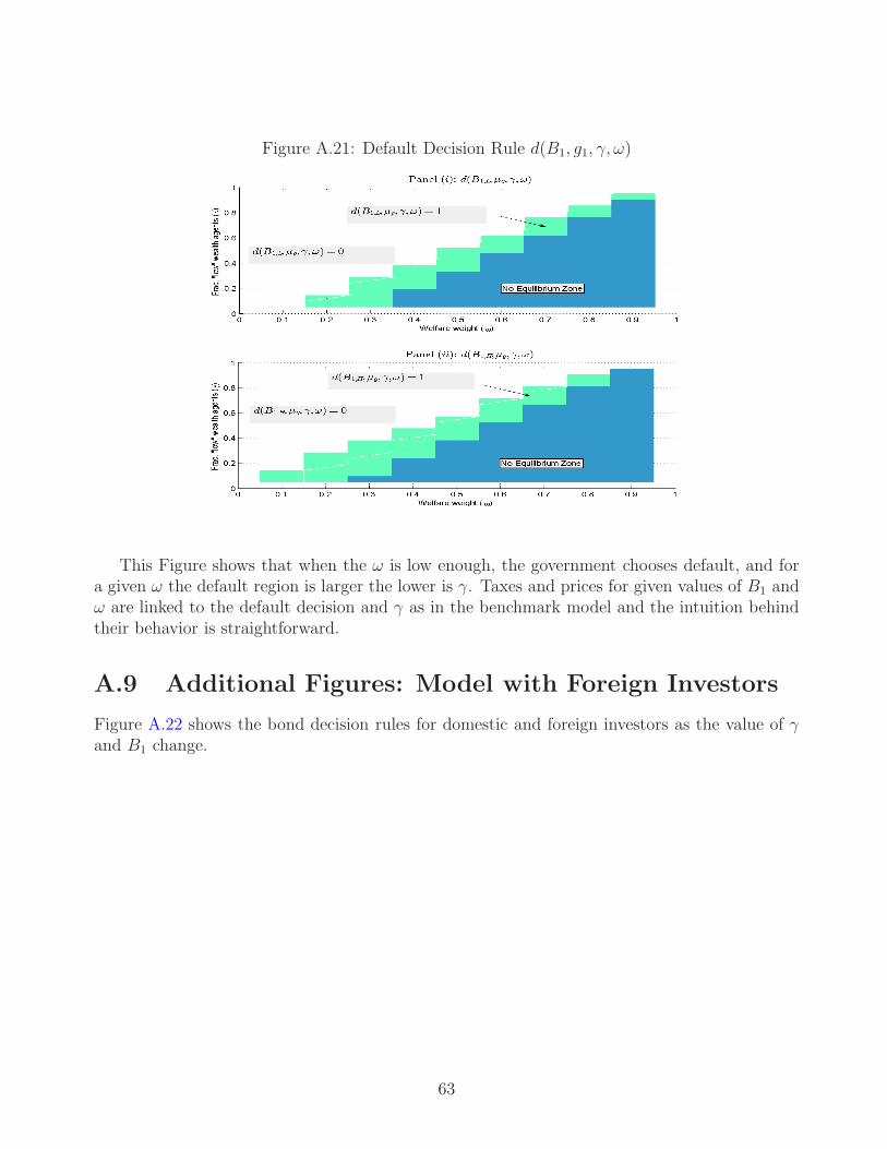
Figure A.21: Default Decision Rule d(B1, g1, γ, ω)

This Figure shows that when the ω is low enough, the government chooses default, and fora given ω the default region is larger the lower is γ. Taxes and prices for given values of B1 andω are linked to the default decision and γ as in the benchmark model and the intuition behindtheir behavior is straightforward.

A.9 Additional Figures: Model with Foreign Investors

Figure A.22 shows the bond decision rules for domestic and foreign investors as the value of γand B1 change.

63

Figure A.22: Decision Rule Domestic and Foreign Agents

0 0.2 0.4 0.6 0.8 10

0.5

1

1.5

2

2.5


bH1 (B1,L, γ)

bH1 (B1,M , γ)

bH1 (B1,H , γ)

0 0.2 0.4 0.6 0.8 1−1

−0.5

0

0.5

1


bL1 (B1,L, γ)

bL1 (B1,M , γ)

bL1 (B1,H , γ)

0 0.2 0.4 0.6 0.8 10

0.05

0.1

0.15

0.2


Bd1(B1,L, γ)

Bd1(B1,M , γ)

Bd1(B1,H , γ)

0 0.2 0.4 0.6 0.8 1−0.15

−0.1

−0.05

0

0.05


Bf1 (B1,L, γ)

Bf1 (B1,M , γ)

Bf1 (B1,H , γ)

Figure A.23 presents the optimal domestic and foreign demand (Panel (i)) and the optimaldebt issuance of the government (Panel (ii)). This Panel also marks with red squares the debtlevels where there is positive risk of default and shows that the feature of equilibrium domesticdefault is also robust to the introduction of foreign lenders.

64

Figure A.23: Equilibrium Domestic and Foreign Debt Holdings

0 0.1 0.2 0.3 0.4 0.5 0.6 0.7 0.8 0.9 1−0.05

0

0.05

0.1

0.15


Panel (i): Domestic and Foreign Positions

Bd1 (γ)

Bf1 (γ)

0 0.1 0.2 0.3 0.4 0.5 0.6 0.7 0.8 0.9 10

0.05

0.1


Panel (ii): B1(γ)

B1(γ)

Def. Ind.

Panel (i) of Figure A.23 shows that domestic (foreign) demand is an increasing (decreasing)function of γ. Panel (ii) of Figure A.23 shows that the debt choice of the government is a concavefunction of γ. This is a direct result of default incentives. When γ is low the government hasstrong incentives to default of foreign lenders, so debt issuance remains low. As γ increases anddomestic households increase their demand for sovereign debt, forces for a “foreign” default de-crease and higher debt levels are attainable. As higher levels of γ, “domestic” default incentivesconstraint the government to increase the debt further and the optimal choice decreases.

A.10 Details for the Model with Two Assets

We now extend the baseline model by allowing domestic agents to save using a risk-free asset, inaddition to government bonds. In particular, agents have access to a non-stochastic productiontechnology yit = z(ki

t)θ with 0 < θ < 1, where yit is total output and ki

t is capital for agentof type i in period t, respectively. The initial aggregate level of capital is denoted by K0. Asbefore, there is a fraction γ of L−type agents that are endowed with bL0 and kL

0 units of domesticsovereign debt and capital respectively. A fraction (1 − γ) of agents are of the H − type and

have endowments given by bH0 =B0−γbL0(1−γ)

and kH0 =

K0−γkL0(1−γ)

. We assume that capital depreciatesat rate δ. At period 0, agents choose how much of their savings they want to allocate to publicbonds bi1 ≥ 0 and capital ki

1 ≥ 0.

65

The assumptions we made above to introduce the second asset, particularly the curvatureof the production function, serve the purpose of supporting a well-defined portfolio choice forprivate agents (i.e. the fraction of wealth to allocate to bonds and capital), which is in turn usefulto solve the government’s problem.41 This formulation is also helpful because it approximatesthe cases in which agents could buy a foreign risk-free asset or a domestic asset that is in zeronet supply (and is also risk free). If, for example, agents could buy a foreign risk-free asset, wecould obtain well defined portfolios by introducing adjustment costs.

The agents’ budget constraint in the initial period is:

ci0 + q0bi1 + ki

1 = z(ki0)

θ + ki0(1− δ) + bi0 − τ0 for i = L,H. (A.32)

The budget constraints in period 1 for the case of no-default and default are:

ci,d=01 = z(ki

1)θ + ki

1(1− δ) + bi1 − τ1 for i = L,H. (A.33)

ci,d=11 = (1− φ(g1))z(k

i1)

θ + ki1(1− δ)− τ1 for i = L,H. (A.34)

The first-order condition with respect to bi1 is

u′(ci0) ≥ (β/q0)Eg1

[u′(ci,d=0

1 )(1− d1)], = if bi1 > 0.

As in the benchmark, the marginal benefit of an extra unit of domestic bond is positive onlyin those states where the government chooses to repay. Similarly, the first-order condition withrespect to capital is given by

u′(ci0) ≥ βEg1

[u′(ci,d=0

1 )(1− d1) + u′(ci,d=11 )d1

] [θz(ki

1)θ−1 + 1− δ

], = if ki

1 > 0.

Since the asset is risk-free, the marginal benefit of an extra unit of capital is positive in all possiblefuture states of the world. However, it will be more valuable in those states where the governmentchooses to default since the marginal utility is higher. These first-order conditions also showthat the level of government debt B1 (as well as the initial wealth dispersion γ) influence theindividual asset demand through the default decision directly, and indirectly through the bondprice.

When the borrowing constraint on bonds binds, this introduces a wedge between the agents’expected marginal product of capital and the expected return on the bond. However, if bothdecisions are interior (which is likely to happen forH−type agents), agents equalize the expectedreturn across assets, which implies:

q0

[θz(ki1)

θ−1 + 1− δ]−1 =

Eg1

[u′(ci,d=0

1 )(1− d1)]

Eg1

[u′(ci,d=0

1 )(1− d1) + u′(ci,d=11 )d1

] . (A.35)

This equation shows that when capital and bond decisions are interior, the wedge between

41This statement is of course conditional on parameters supporting the interesting case in which at least someagents do hold both assets at equilibrium.

66

the price of the bond and the marginal productivity of capital is driven uniquely by defaultrisk (weighted by marginal utility in each state of the world). In the particular case in whichin addition we are in a combination of B1 and γ where there is no default risk, the optimalindividual choice of capital is given by:

(1/q0) = (αz(ki1)

α−1 + 1− δ)

⇒ ki1 =

[αzq0

1− q0(1− δ)

] 11−α

.

The demand for capital increases with the price of the bond, or falls with the interest rate, asin standard investment models.

In this environment, the government faces similar budget constraints to those presented inthe benchmark model. However, when choosing the optimal level of debt and whether to defaultor not, it takes into account not only the distribution of bond holdings across agents but alsothe distribution of capital. In particular, at t = 1, the repayment value is given by:

W d=01 (B1, g1, γ) = γu(z(kL

1 )θ+(1−δ)kL

1 −g1+bL1 −B1)+(1−γ)u(z(kH1 )

θ+(1−δ)kH1 −g1+bH1 −B1)

and the value of default is

W d=11 (g1, γ) = γu(z(kL

1 )θ(1−φ(g1))+(1−δ)kL

1 −g1)+(1−γ)u(z(kH1 )

θ(1−φ(g1))+(1−δ)kH1 −g1).

Note that in each case, the individual capital and bond decisions {bi1, ki1} are a function of B1 and

γ. This implies that the variance of consumption, a key moment to determine the differentialvalue of repayment v. default, is a function of the amount of debt the government has issued inperiod 0.

The model seems simple, but its solution needs to be obtained numerically. To make thiscase as close as possible to the benchmark model, we assume that ki

0 = K0 (i.e. all initialheterogeneity is in initial bond holdings). Still, this results in heterogeneous bond and capitalholdings in the second period. We set z to normalize GDP to 1, θ equal to 0.33 (a standardvalue), δ = 0.10 and set K0 so the capital to output ratio is equal to 2. All other parametersare set equal to those in the benchmark.

Figure A.24 presents the decision rules of the model. The top panels correspond to thosefor the H−type and the bottom panels to those for the L − type. They are truncated forcombinations of B1 and γ where the equilibrium does not exist because the government defaultsfor all possible realizations of g1.

67

Figure A.24: Bond and Capital Decision Rules in Model with Two Assets

0 0.2 0.4 0.6 0.8 11

1.5

2

2.5

3

3.5

4


kH1 (B1,L, γ)

kH1 (B1,M , γ)

kH1 (B1,H , γ)

0 0.2 0.4 0.6 0.8 10

0.2

0.4

0.6

0.8


bH1 (B1,L, γ)

bH1 (B1,M , γ)

bH1 (B1,H , γ)

0 0.2 0.4 0.6 0.8 10.95

1

1.05

1.1

1.15

1.2


kL1 (B1,L, γ)

kL1 (B1,M , γ)

kL1 (B1,H , γ)

0 0.2 0.4 0.6 0.8 1−1

−0.5

0

0.5

1


bL1 (B1,L, γ)

bL1 (B1,M , γ)

bL1 (B1,H , γ)

As in the benchmark model, L − type agents are at the borrowing constraint for all valuesof B1. Their capital choice is determined completely by the first-order condition for capital. Aswe get close to a region with default risk, their demand for capital decreases since the marginalbenefit of an extra unit of savings decreases, because they expect to receive a transfer in thecase of a default. On the other hand, H−type agents are never at the borrowing constraint,so their choice of capital is given by equation (A.35). As in the benchmark economy with oneasset, while default risk is low (B1 = B1,L), the bond price increases with γ to induce theH−type to demand a decreasing fraction of their initial bond position (but still increasing inγ). This increase in bond prices drives the increasing demand for capital for the H−type whenB1 = B1,L. As we move to higher levels of B1, similar factors are at play but since default risk isnot trivially small, bond prices do not rise as fast, inducing a relatively flat demand for capitalwith slightly increasing demand for domestic bonds for H−types with a decreasing demand forcapital for L−types.

68

Figure A.25: Equilibrium Model with Two Assets

0 0.5 10

0.05

0.1

0.15



1(γ)

B∗

1(γ)

BRF1 (γ)

Def. Ind

0 0.5 10.85

0.9

0.95

1



1(γ), γ)

q(B∗

1(γ))

1/mpkH

0 0.5 10

0.5

1

1.5

2



spre

ad

(%

)

0 0.5 10

0.005

0.01

0.015



1(γ), γ)

Note: mpkH denotes the marginal product of capital for the H−type and is given byθz(kH)θ−1 + 1− δ. The spread is computed as 1/q(B1, γ) −mpkH .

Figure A.25 presents the equilibrium functions as they vary with γ. As before, we presentthe optimal debt choice of the government, and the associated bond prices, spreads (measuredagainst the marginal product of capital of the H−type) and the default probability.42 This figureshows that the results of the benchmark model are robust to the introduction of an additionalasset.

Panel (i) shows that optimal debt falls as γ increases and Panel (iv) that default risk isnot zero for γ > 0.20 (non negligible for γ > 0.50). Importantly, the probability of a defaultevent is increasing in the initial level of wealth inequality. As default risk increases, the wedgebetween the marginal product of capital and the equilibrium bond price increases driving upthe spreads (see Panels (ii) and (iii)). Different from our baseline model, bond prices remainbelow 1, implying positive real interest payments for all values of γ.

Figure A.26 compares the equilibrium functions of the benchmark model with those of theeconomy with two assets.

42We measure spreads against the marginal product of capital of the H−type since the wedge is only driven bydefault risk. In the case of the L−type agents there is an additional component that arises from the multiplieron the non negativity constraint on domestic bonds.

69

Figure A.26: Comparison Equilibrium Benchmark vs Two Asset Model

0 0.5 10

0.05

0.1

0.15

0.2



1(γ)

0 0.5 10

1

2

3

4



1(γ), γ)

BenchmarkTwo Assets

0 0.5 1−0.5

0

0.5

1

1.5

2



spre

ad

(%

)

0 0.5 10

0.005

0.01

0.015

0.02



1(γ), γ)

The model with two assets sustains higher levels of debt, but as default risk increases thegovernment chooses to reduce debt issuance faster in the economy with capital than in thebenchmark. Even though we observe a lower default probability and spreads, the previousresult derives from the fact that lower levels of debt are sustainable when agents have accessto another asset. The cost of a default is not as high for the H−types and a default reducesconsumption dispersion that increases faster with γ in the economy with capital than in thebenchmark since initial dispersion is amplified via capital.

70

DISTRIBUTIONAL INCENTIVES IN AN EQUILIBRIUM MODEL OF ... · Distributional Incentives in an...

Documents

Transcript of DISTRIBUTIONAL INCENTIVES IN AN EQUILIBRIUM MODEL OF ... · Distributional Incentives in an...