DISTRIBUTION SYSTEM OPTIMIZATION WITH INTEGRATED ...

University of Kentucky University of Kentucky

UKnowledge UKnowledge

Theses and Dissertations--Electrical and Computer Engineering Electrical and Computer Engineering

2018

DISTRIBUTION SYSTEM OPTIMIZATION WITH INTEGRATED DISTRIBUTION SYSTEM OPTIMIZATION WITH INTEGRATED

DISTRIBUTED GENERATION DISTRIBUTED GENERATION

Sarmad Khaleel Ibrahim University of Kentucky, [email protected] Digital Object Identifier: https://doi.org/10.13023/ETD.2018.132

Right click to open a feedback form in a new tab to let us know how this document benefits you. Right click to open a feedback form in a new tab to let us know how this document benefits you.

Recommended Citation Recommended Citation Ibrahim, Sarmad Khaleel, "DISTRIBUTION SYSTEM OPTIMIZATION WITH INTEGRATED DISTRIBUTED GENERATION" (2018). Theses and Dissertations--Electrical and Computer Engineering. 116. https://uknowledge.uky.edu/ece_etds/116

This Doctoral Dissertation is brought to you for free and open access by the Electrical and Computer Engineering at UKnowledge. It has been accepted for inclusion in Theses and Dissertations--Electrical and Computer Engineering by an authorized administrator of UKnowledge. For more information, please contact [email protected].

http://uknowledge.uky.edu/

http://uknowledge.uky.edu/

https://uknowledge.uky.edu/

https://uknowledge.uky.edu/ece_etds

https://uknowledge.uky.edu/ece_etds

https://uknowledge.uky.edu/ece

https://uky.az1.qualtrics.com/jfe/form/SV_9mq8fx2GnONRfz7

mailto:[email protected]

STUDENT AGREEMENT: STUDENT AGREEMENT:

I represent that my thesis or dissertation and abstract are my original work. Proper attribution

has been given to all outside sources. I understand that I am solely responsible for obtaining

any needed copyright permissions. I have obtained needed written permission statement(s)

from the owner(s) of each third-party copyrighted matter to be included in my work, allowing

electronic distribution (if such use is not permitted by the fair use doctrine) which will be

submitted to UKnowledge as Additional File.

I hereby grant to The University of Kentucky and its agents the irrevocable, non-exclusive, and

royalty-free license to archive and make accessible my work in whole or in part in all forms of

media, now or hereafter known. I agree that the document mentioned above may be made

available immediately for worldwide access unless an embargo applies.

I retain all other ownership rights to the copyright of my work. I also retain the right to use in

future works (such as articles or books) all or part of my work. I understand that I am free to

register the copyright to my work.

REVIEW, APPROVAL AND ACCEPTANCE REVIEW, APPROVAL AND ACCEPTANCE

The document mentioned above has been reviewed and accepted by the student’s advisor, on

behalf of the advisory committee, and by the Director of Graduate Studies (DGS), on behalf of

the program; we verify that this is the final, approved version of the student’s thesis including all

changes required by the advisory committee. The undersigned agree to abide by the statements

above.

Sarmad Khaleel Ibrahim, Student

Dr. Aaron M. Cramer, Major Professor

Dr. Caicheng Lu, Director of Graduate Studies

DISTRIBUTION SYSTEM OPTIMIZATION WITH INTEGRATED DISTRIBUTEDGENERATION

DISSERTATION

A dissertation submitted in partial fulfillment of therequirements for the degree of Doctor of Philosophy in the

College of Engineering at the University of Kentucky

By

Sarmad Khaleel Ibrahim

Lexington, Kentucky

Director: Dr. Aaron M. Cramer , Associate Professor of Electrical Engineering

Lexington, Kentucky

2018

Copyright© Sarmad Khaleel Ibrahim 2018

ABSTRACT OF DISSERTATION


In this dissertation, several volt-var optimization methods have been proposed to improvethe expected performance of the distribution system using distributed renewable energysources and conventional volt-var control equipment:photovoltaic inverter reactive powercontrol for chance-constrained distribution system performance optimisation, integrateddistribution system optimization using a chance-constrained formulation, integrated con-trol of distribution system equipment and distributed generation inverters, and coordinationof PV inverters and voltage regulators considering generation correlation and voltage qual-ity constraints for loss minimization. Distributed generation sources (DGs) have importantbenefits, including the use of renewable resources, increased customer participation, anddecreased losses. However, as the penetration level of DGs increases, the technical chal-lenges of integrating these resources into the power system increase as well. One suchchallenge is the rapid variation of voltages along distribution feeders in response to DGoutput fluctuations, and the traditional volt-var control equipment and inverter-based DGcan be used to address this challenge.

These methods aim to achieve an optimal expected performance with respect to thefigure of merit of interest to the distribution system operator while maintaining appropriatesystem voltage magnitudes and considering the uncertainty of DG power injections. Thefirst method is used to optimize only the reactive power output of DGs to improve systemperformance (e.g., operating profit) and compensate for variations in active power injectionwhile maintaining appropriate system voltage magnitudes and considering the uncertaintyof DG power injections over the interval of interest. The second method proposes an inte-grated volt-var control based on a control action ahead of time to find the optimal voltageregulation tap settings and inverter reactive control parameters to improve the expectedsystem performance (e.g., operating profit) while keeping the voltages across the systemwithin specified ranges and considering the uncertainty of DG power injections over theinterval of interest. In the third method, an integrated control strategy is formulated forthe coordinated control of both distribution system equipment and inverter-based DG. Thiscontrol strategy combines the use of inverter reactive power capability with the operationof voltage regulators to improve the expected value of the desired figure of merit (e.g., sys-tem losses) while maintaining appropriate system voltage magnitudes. The fourth method

proposes a coordinated control strategy of voltage and reactive power control equipment toimprove the expected system performance (e.g., system losses and voltage profiles) whileconsidering the spatial correlation among the DGs and keeping voltage magnitudes withinpermissible limits, by formulating chance constraints on the voltage magnitude and con-sidering the uncertainty of PV power injections over the interval of interest.

The proposed methods require infrequent communication with the distribution systemoperator and base their decisions on short-term forecasts (i.e., the first and second meth-ods) and long-term forecasts (i.e., the third and fourth methods). The proposed methodsachieve the best set of control actions for all voltage and reactive power control equipmentto improve the expected value of the figure of merit proposed in this dissertation withoutviolating any of the operating constraints. The proposed methods are validated using theIEEE 123-node radial distribution test feeder.

KEYWORDS: Distributed power generation, chance-constrained programming, renew-able integration, reactive power optimization, voltage control

Sarmad Khaleel IbrahimAuthor’s signature

May 4, 2018Date


By

Sarmad Khaleel Ibrahim

Aaron M. CramerDirector of Dissertation

Caicheng LuDirector of Graduate Studies

May 4, 2018Data

To my parents and family.

ACKNOWLEDGEMENTS

To my advisor Dr. Aaron M. Cramer, thank you for the advice and support. I have been

lucky to work with Dr. Cramer for the past four years. I would also like to thank Dr. Liao

for providing help, ideas, and co-authoring a couple of papers with me. I would like to

thank my committee members Dr. Yuan Liao, Dr. Paul A. Dolloff, and Dr. Joseph Sottile

for their insightful comments and their advice and willingness to serve on my dissertation

advisory committee. I have to thank my outside examiner Prof. Zongming Fei for his

valuable time. I would like to thank my wife for her encouragement and support through

my Ph.D. studies. I have to thank my parents for their support and encouragement. They

are always supporting me and encouraging me with their best wishes. This work was

supported by the Ministry of Higher Education and Scientific Research and the University

of Babylon, Iraq.

iii

TABLE OF CONTENTS

Acknowledgements . . . . . . . . . . . . . . . . . . . . . . . . . . . . . . . . . . iii

Table of Contents . . . . . . . . . . . . . . . . . . . . . . . . . . . . . . . . . . . iv

List of Tables . . . . . . . . . . . . . . . . . . . . . . . . . . . . . . . . . . . . . . vi

List of Figures . . . . . . . . . . . . . . . . . . . . . . . . . . . . . . . . . . . . . vii

1 Introduction . . . . . . . . . . . . . . . . . . . . . . . . . . . . . . . . . . . . 11.1 Introduction . . . . . . . . . . . . . . . . . . . . . . . . . . . . . . . . . . 11.2 Distributed Generator Sources (DGs) . . . . . . . . . . . . . . . . . . . . 11.3 The Challenges Associated with Integration of DGs . . . . . . . . . . . . . 21.4 The Benefits Associated with Integration of DGs . . . . . . . . . . . . . . 31.5 Volt-var Control in Distribution Systems with DGs . . . . . . . . . . . . . 31.6 Dissertation Outline . . . . . . . . . . . . . . . . . . . . . . . . . . . . . . 6

2 Literature Review . . . . . . . . . . . . . . . . . . . . . . . . . . . . . . . . . 7

3 Photovoltaic Inverter Reactive Power Control for Chance-Constrained Dis-tribution System Performance Optimisation . . . . . . . . . . . . . . . . . . . 133.1 Introduction . . . . . . . . . . . . . . . . . . . . . . . . . . . . . . . . . . 133.2 System Description and Approximation . . . . . . . . . . . . . . . . . . . 143.3 Problem Formulation . . . . . . . . . . . . . . . . . . . . . . . . . . . . . 173.4 Test System Description . . . . . . . . . . . . . . . . . . . . . . . . . . . . 223.5 Simulation Results and Discussion . . . . . . . . . . . . . . . . . . . . . . 25

3.5.1 Case 1 (Cloudy) . . . . . . . . . . . . . . . . . . . . . . . . . . . . 293.5.2 Case 2 (Sunny) . . . . . . . . . . . . . . . . . . . . . . . . . . . . 303.5.3 Case 3 (Transient) . . . . . . . . . . . . . . . . . . . . . . . . . . . 323.5.4 Sensitivity to Distribution Assumptions . . . . . . . . . . . . . . . 35

3.6 Conclusion . . . . . . . . . . . . . . . . . . . . . . . . . . . . . . . . . . 36

4 Integrated Distribution System Optimization Using a Chance-ConstrainedFormulation . . . . . . . . . . . . . . . . . . . . . . . . . . . . . . . . . . . . 384.1 Introduction . . . . . . . . . . . . . . . . . . . . . . . . . . . . . . . . . . 384.2 System Description and Approximation . . . . . . . . . . . . . . . . . . . 394.3 Problem Formulation . . . . . . . . . . . . . . . . . . . . . . . . . . . . . 414.4 Description of the distribution system and case studies . . . . . . . . . . . 474.5 Simulation results . . . . . . . . . . . . . . . . . . . . . . . . . . . . . . . 484.6 Conclusion . . . . . . . . . . . . . . . . . . . . . . . . . . . . . . . . . . 50

iv

5 Integrated Control of Voltage Regulators and Distributed Generation In-verters . . . . . . . . . . . . . . . . . . . . . . . . . . . . . . . . . . . . . . . . 525.1 Introduction . . . . . . . . . . . . . . . . . . . . . . . . . . . . . . . . . . 525.2 System Description and Approximation . . . . . . . . . . . . . . . . . . . 535.3 Problem Formulation . . . . . . . . . . . . . . . . . . . . . . . . . . . . . 565.4 Test System Description . . . . . . . . . . . . . . . . . . . . . . . . . . . . 625.5 Simulation Results and Discussion . . . . . . . . . . . . . . . . . . . . . . 66

5.5.1 Sensitivity to Distribution Assumptions . . . . . . . . . . . . . . . 745.6 Conclusion . . . . . . . . . . . . . . . . . . . . . . . . . . . . . . . . . . 77

6 Coordination of PV Inverters and Voltage Regulators Considering Genera-tion Correlation and Voltage Quality Constr-aints for Loss Minimization . . . . . . . . . . . . . . . . . . . . . . . . . . . . 796.1 Introduction . . . . . . . . . . . . . . . . . . . . . . . . . . . . . . . . . . 796.2 System Description and Approximation . . . . . . . . . . . . . . . . . . . 816.3 Problem Formulation . . . . . . . . . . . . . . . . . . . . . . . . . . . . . 816.4 Test System Description . . . . . . . . . . . . . . . . . . . . . . . . . . . . 866.5 Simulation Results and Discussion . . . . . . . . . . . . . . . . . . . . . . 896.6 Conclusion . . . . . . . . . . . . . . . . . . . . . . . . . . . . . . . . . . 97

7 Conclusion and Future Work . . . . . . . . . . . . . . . . . . . . . . . . . . . 987.1 Conclusion . . . . . . . . . . . . . . . . . . . . . . . . . . . . . . . . . . 987.2 Future Work . . . . . . . . . . . . . . . . . . . . . . . . . . . . . . . . . . 102

Bibliography . . . . . . . . . . . . . . . . . . . . . . . . . . . . . . . . . . . . . . 105

Vita . . . . . . . . . . . . . . . . . . . . . . . . . . . . . . . . . . . . . . . . . . . 113

v

LIST OF TABLES

3.1 Inverter parameters . . . . . . . . . . . . . . . . . . . . . . . . . . . . . . . . 243.2 Voltage regulator tap settings . . . . . . . . . . . . . . . . . . . . . . . . . . . 283.3 Simulation results for Case 1 (Cloudy) . . . . . . . . . . . . . . . . . . . . . . 293.4 Simulation results for Case 2 (Sunny) . . . . . . . . . . . . . . . . . . . . . . 303.5 Simulation results for Case 3 (Transient) . . . . . . . . . . . . . . . . . . . . . 343.6 Performance of proposed method for Case 3 (Transient) . . . . . . . . . . . . . 35

4.1 Simulation Results for Cases . . . . . . . . . . . . . . . . . . . . . . . . . . . 49

5.1 Inverter parameters . . . . . . . . . . . . . . . . . . . . . . . . . . . . . . . . 645.2 Simulation Results for All Instances . . . . . . . . . . . . . . . . . . . . . . . 675.3 The tap change operations of DM and IM versions over the interval of interest . 725.4 Accuracy of the proposed method (i.e., optimal solutions) . . . . . . . . . . . . 735.5 The sensitivity of the proposed method (i.e., initial solutions) . . . . . . . . . . 735.6 Performance of IM . . . . . . . . . . . . . . . . . . . . . . . . . . . . . . . . 74

6.1 Simulation results for all methods . . . . . . . . . . . . . . . . . . . . . . . . 906.2 Simulation results for voltage magnitude violations . . . . . . . . . . . . . . . 946.3 Total number of tap change operations of all methods over the interval of interest 96

vi

LIST OF FIGURES

3.1 Flowchart of proposed solution algorithm . . . . . . . . . . . . . . . . . . . . 233.2 IEEE 123-node radial distribution test feeder. The PV source location nodes

are indicated with PV panels. . . . . . . . . . . . . . . . . . . . . . . . . . . . 253.3 Irradiance data for (a) Case 1 (Cloudy), (b) Case 2 (Sunny), and (c) Case 3

(Transient). . . . . . . . . . . . . . . . . . . . . . . . . . . . . . . . . . . . . 263.4 Volt/var control using droop control function. . . . . . . . . . . . . . . . . . . 273.5 Node 83 a-phase voltage magnitude for (a) Case 1 (Cloudy), (b) Case 2 (Sunny),

and (c) Case 3 (Transient), and (d) Node 65 a-phase voltage magnitude forCase 3 (Transient). . . . . . . . . . . . . . . . . . . . . . . . . . . . . . . . . 31

3.6 Sample of PV inverter active power set points in (a) and optimal reactive powerset points in (b) for a time interval at Node 1 for a-phase, b-phase, and c-phasefor the CCO method in Case 3 (Transient). . . . . . . . . . . . . . . . . . . . . 32

4.1 Flowchart of proposed solution algorithm . . . . . . . . . . . . . . . . . . . . 464.2 Node 65 a-phase voltage magnitude for (a) Case 3 (Transient) and Node 83

a-phase voltage magnitude for (b) Case 3 (Transient). . . . . . . . . . . . . . . 50

5.1 Flowchart of proposed solution algorithm . . . . . . . . . . . . . . . . . . . . 635.2 Load profile and PV active power injection. . . . . . . . . . . . . . . . . . . . 655.3 (a) Node 114 a-phase voltage magnitude for SM, (b) Node 104 c-phase voltage

magnitude for DMV1 and DMV2, (c) Node 114 a-phase voltage magnitude forIMV1 and IMV2, and (d) Node 104 c-phase voltage magnitude for DMV3 andIMV3. . . . . . . . . . . . . . . . . . . . . . . . . . . . . . . . . . . . . . . . 69

5.4 Losses for DMV1 and IMV3. . . . . . . . . . . . . . . . . . . . . . . . . . . . 705.5 (a) Tap positions for the voltage regulator connected to Node 160 for IMV3,

(b) PV inverter three-phase reactive power injection at Node 55, and (c) and(d) the PV inverter three-phase fixed and variable reactive power injection (αααand βββ ) at Node 55 for IMV3. . . . . . . . . . . . . . . . . . . . . . . . . . . . 71

5.6 (a) Node 114 a-phase voltage magnitude for synthetic and actual case of theIMV1, (b) Node 114 a-phase voltage magnitude for synthetic and actual caseof the IMV2, and (c) Node 114 a-phase voltage magnitude for for syntheticand actual case of the IMV3. . . . . . . . . . . . . . . . . . . . . . . . . . . . 75

6.1 (a) Node 104 c-phase voltage magnitude for BM and LCIM, (b) Node 104 c-phase voltage magnitude for the DM and LCIM, (c) Node 114 a-phase voltagemagnitude for the IM and LIM, and (d) Node 114 a-phase voltage magnitudefor the CIM and LCIM. . . . . . . . . . . . . . . . . . . . . . . . . . . . . . . 93

6.2 The worst 15-minute standard deviation of voltage magnitude of Node 114 a-phase voltage magnitude for the CIM and LCIM in (a) and for the IM and LIMin (b). . . . . . . . . . . . . . . . . . . . . . . . . . . . . . . . . . . . . . . . 95

vii

6.3 Tap positions for the voltage regulator connected to Node 160 for the CIM in(a) and for the LCIM in (b). . . . . . . . . . . . . . . . . . . . . . . . . . . . . 96

viii

Chapter 1Introduction

1.1 Introduction

A traditional power distribution system is a part of a power delivery system which serves

as a link between the transmission system and customers. It has been initially designed

and operated based on many essential assumptions in which the reliability and efficiency

of distribution systems can be evaluated by designers or customers. It is designed to deliver

power from the high voltage side of the electrical grid to last customers connected on the

low voltage side. It is also designed based on unidirectional power flow, low energy losses,

minimum consumption, voltages and currents within allowable limits, and centralized gen-

erating [1]. Although non-renewable energy sources are considered the primary source of

energy in most electric power systems, they are also considered a source of environmental

pollution because of waste materials such as carbon dioxide and sulfur dioxide, which con-

tribute to increasing rates of greenhouse gas emissions in our atmosphere. Greenhouse gas

emissions and polluting materials have necessitated research into new sources of produc-

ing electricity with less environmental impact. Renewable energy is an efficient solution to

reduce global warming.

1.2 Distributed Generator Sources (DGs)

The increase of environmental pollution produced from conventional energy resources has

stimulated the electric utilities to think of alternative energy sources to improve the tra-

1

ditional electric power system. This necessity of finding alternative energy sources with

less environmental impact and production cost has dramatically increased in recent years.

This need also gives a motivation to look for new small and large-scale power generation

technologies that are able to be located at any point of consumption to reduce resources

and improve system performance. These generating techniques are known as distributed

generation or renewable energy distributed generation sources and can be easily installed

into distribution systems by customers or electric utilities. However, these power genera-

tion sources fluctuate over the course of the day because they can only produce electricity

when their energy source is available [2].

1.3 The Challenges Associated with Integration of DGs

When the number of DGs, which are mostly connected near the loads, increases with a

high-level penetration, the challenges of integrating DGs into a power grid increase as

well. With both a bidirectional power flow and fluctuated nature of DGs that cause a

voltage fluctuation [3], the imperative challenge is how to control and mitigate the adverse

effects of DGs such as a maximum voltage deviation. Also, all voltage control devices in

traditional distribution systems have been mainly designed to operate without DGs, and

voltage magnitudes decrease along the distribution feeder from the substation to the end-

users. The presence of DGs makes this assumption no longer valid because the change of

power flow (e.g., the bidirectional power flow) causes the node phase voltage magnitudes

along the distribution feeder to violate these assumptions [4].

The DG impacts relatively increase or decrease depending on the location and size of a

penetration level of the DGs generation. These impacts can significantly reduce the life of

equipment that is used in a distribution feeder for controlling issues. Some of the signifi-

cant impacts and challenges have been addressed by researchers for the implementation of

distribution networks with DGs including voltage magnitude levels, power flow, thermal

equipment ratings, fault current levels, and protection issues [5].

2

1.4 The Benefits Associated with Integration of DGs

The contribution of increasing benefits by DGs to the electric utilities is dramatically in-

creased during the last few decades. Most electric utilities have found that the economic

cost of injecting reactive power into distribution systems can be obtained by using DGs,

and efficient use of the DGs will highly benefit the electric utilities. Many advantages

have been mainly obtained by using DGs into distribution systems such as supporting the

network voltage, minimizing feeder losses, increasing the system reliability, and reducing

greenhouse gas emissions [6–8]. The DGs are also capable to assist the energy supply for

distribution system loads. Once DGs are connected near the loads, the electric utilities and

users who own the DGs can obtain some good benefits such as loss reduction and increased

operating profit [9].

1.5 Volt-var Control in Distribution Systems with DGs

The primary advantages of using the volt-var control in distribution systems are to main-

tain appropriate system voltages and consider the uncertainty of power injections and loads

by injecting or consuming reactive power as necessary. In the traditional distribution sys-

tem, volt-var control actions have been performed based on the voltage and reactive power

equipment such as switchable capacitor banks, on load tap changer transformers, and step

voltage regulators. This volt-var control equipment is designed to operate based on as-

sumptions such as unidirectional power flow in which the voltages decrease along the dis-

tribution system within the American National Standards Institute (ANSI) standard.

Coordinated volt-var control methods using the traditional voltage and reactive power

equipment in distribution systems to minimize the energy consumption or system losses

have been widely investigated and studied by researchers. For example, a step voltage

regulator and shunt capacitor are coordinated to keep the system voltage within acceptable

limits under various load conditions [10]. Another researcher has discovered that finding

3

optimal scheduling of on-load tap changer position and capacitor bank status for some

hours in advance can minimize the real power losses [11]. Voltage stability of the system

can be improved by controlling the operational decision of the voltage regulator devices

[12]. Different control approaches in the distribution system are reviewed based on volt-

var control strategies [13].

Due to falling costs and increasing interest in alternative energy sources rather than

fossil-fuel-based sources, using DGs has increased significantly in recent years with the

transmission and distribution system [14]. The connection of DGs into the distribution

system has increased the challenges of traditional volt-var control equipment to match the

assumptions for which the distribution system is designed. With increasing the penetration

level and intermittent nature of DGs, traditional feeder volt-var controls are too slow to

react to fast fluctuations in the power output of DGs. Traditional voltage control systems,

which are considered local static var sources and too expensive, cannot respond to a fast

variation in the power output of DGs [15].

With fast development in DG inverter technologies, the electric utilities have found that

power electronic inverter-based DGs are an excellent alternative to solve the problem as-

sociated with a rapid response to a voltage variation. Since inverter-based DGs are power

electronic devices, they can provide the reactive power needed in less than 50 milliseconds

to avoid fast voltage fluctuations caused by transient cloud passing [16, 17]. Using this

feature, inverter-based DGs have reduced the dependency on the traditional distribution

system control such as on-load tap changers, capacitor banks, and static var compensators.

For example, shunt capacitors can only support the system voltage by injecting reactive

power, but cannot absorb reactive power. On the other hand, DG inverters have fast re-

sponse times and simply provide dynamic values, and can efficiently provide faster and

more flexible reactive power support that is capable of generating or absorbing and assist-

ing in controlling voltage [18].

Coordinated reactive power compensation, which can be obtained from DG inverters

4

and traditional volt-var control devices, can provide significant economic benefits for elec-

tric utilities and can improve the system efficiency and reliability [19, 20]. For example,

significant advantages can be obtained using PV inverters such as minimizing system losses

and increasing line capacities [21]. The optimal volt-var control is proposed using the ca-

pability of PV inverters to generate and absorb the reactive power to minimize system

losses and energy consumption while maintaining the voltage magnitudes within desired

ranges [22].

The volt-var control also aims to keep the voltage deviation within an acceptable range

by using system control devices, such as on-load tap changer transformers and PV invert-

ers, and to regulate voltage magnitudes for either local control or global control along the

distribution feeder [23]. PV inverters can provide a reactive power compensation that can

be utilized in supplying voltage support when fluctuations in generation occur [24]. The

volt-var control can also be used to conserve energy by maintaining the voltage magni-

tudes within acceptable levels [25]. The electric utility company can deliver energy more

efficiently by controlling voltage magnitudes based on the ANSI standards [26]. As a re-

sult, the electric utilities will save money by reducing total power losses in a distribution

feeder [27].

There are many other methods to support voltage optimization in the distribution system

using DGs. Many electric utility companies have efficiently used an accurate power pre-

diction method for fluctuating solar power production to improve the accuracy of volt-var

control methods. An accurate prediction is essential for electric utilities because efficient

use of the fluctuating solar power production could provide a strong economic impact on

total generation costs and a substantial improvement associated with the integration of DGs

into the distribution feeder [28].

This dissertation provides supervisory control methods focusing on improving the ex-

pected system performance concerning a figure of the merit of interest to the distribution

system operator (e.g., operating profits, system losses, and voltage profiles) while con-

5

straining the probability of unacceptable voltage magnitudes occurring during the interval

of interest. The integrated control strategies proposed herein are used to coordinate exist-

ing inverter-based DG and voltage control equipment (e.g., voltage regulators) based on

the current communication infrastructure of traditional power distribution networks. For

instance, it is assumed that supervisory control and data acquisition (SCADA) systems can

be used for communicating and coordinating between the distribution system operator and

the available voltage and reactive power control equipment. These control strategies also

require both infrequent communication with the distribution system operator and infre-

quent changes to voltage control equipment. However, they can respond to rapidly chang-

ing conditions by providing control parameters to the inverters to allow them to respond to

such changes in real time, a capability that is available in smart inverters.

1.6 Dissertation Outline

The remainder of this dissertation is organized as follows: The literature review related to

the contribution of DG inverters and traditional voltage regulator devices in volt-var con-

trol methods into the distribution system is described in Chapter 2. Photovoltaic inverter

reactive power control for chance-constrained distribution system performance optimisa-

tion is proposed in Chapter 3. Integrated distribution system optimization using a chance-

constrained formulation is discussed in Chapter 4. Integrated control of distribution system

equipment and distributed generation inverters is discussed in Chapter 5. Coordination of

PV inverters and voltage regulators considering generation correlation and voltage quality

constraints for loss minimization is discussed in Chapter 6. Conclusions and the future

work are discussed in Chapter 7.

6

Chapter 2Literature Review

With more PV installations being implemented in distribution systems, due to falling costs

and increasing interest in alternative energy sources rather than fossil-fuel-based sources,

the technical challenges associated with high penetration levels are becoming ever more

critical [29]. Despite the potential benefits of DGs [30], such as PV and wind generation,

high penetration of these resources also reduces the effectiveness of existing methods that

are used to maintain system voltage magnitudes and reduce system losses in distribution

systems [31]. Mitigation of the problems associated with the intermittency of PV sources

when clouds pass is a difficult technical challenge that distribution system operators must

address. PV output changes both over the course of a day and much shorter periods due to

cloud transient. Cloud transient caused by the passage of shadows over a PV source can

result in changes in solar irradiance as much as 60%/s [32, 33]. Therefore, PV inverters,

which perform maximum power point tracking on the order of 50 milliseconds [16, 34],

will quickly vary the amount of active power being injected into the distribution system.

These transients cause voltage magnitudes in distribution systems to fluctuate rapidly. The

rapid variation of voltages along distribution feeders in response to PV output fluctuations

remains one of the challenges that has increased with rising PV penetration levels in the

distribution feeder [35]. While facing this issue, distribution system operators are still

charged with improving system performance by reducing system losses or total demand.

Many studies have proposed that PV inverters, with their reactive power capability that

7

can be largely controlled independently [36], can be used to improve distribution system

operations [37, 38]. PV inverters, in addition to feeding active power, are capable of ab-

sorbing reactive power from or providing it to the distribution system [39]. PV inverters,

unlike other distribution system devices, are necessary to inject power from PV sources

into the distribution system and are typically purchased by the PV owner. PV inverters can

efficiently reduce the dependency on traditional distribution system control equipment such

as OLTC transformers, capacitor banks, and static var compensators [31, 40]. Traditional

voltage regulator devices either do not have the capability to respond to voltage fluctua-

tions, due to fast variation in the power output of PV sources (in the case of mechanical

devices), or are very expensive (in the case of power electronic devices) [41]. Many pub-

lished studies have addressed the use of static var compensators, capacitor banks, on-load

tap changer transformers (OLTC), etc., for volt-var optimization [42,43]. A voltage and var

control (VCC) with DGs is used to find the optimal setting for the feeder control variables

using traditional voltage control and a PV inverter [44].

Many studies have proposed that PV inverters and traditional volt-var control devices

can provide significant economic benefits for electric utilities and can improve the system

efficiency and reliability. For example, improving the operating profit using the distribution

system losses and the voltage profile as important factors to measure the growth in the oper-

ating profit is shown in [45–47]. The goodness factor of DGs based on the calculation of the

incremental contribution of DGs to distribution system losses is proposed in [45]. Increas-

ing financial benefits and managing the load demand by optimizing short-term activities for

a distribution system operator is considered in [46]. Financial benefits can be obtained by

using the nodal pricing on the distribution network [47]. The PV inverters can be used to

improve the efficiency of power distribution systems by reducing line losses. For example,

in [48], a decentralized controller is proposed to reduce system losses by controlling the

reactive power being injected by PV inverters. System losses can be reduced by injecting

most of the PV power produced into the phase with the highest power consumption [49].

8

In [50], a real-time volt-var controller is proposed to reduce feeder losses by controlling

the traditional voltage regulation devices along with a PV inverter. The integration of DGs

used to maximize the system performance and maintain a voltage regulation with uncertain

power injections is presented in [51, 52]. Minimizing the operating cost and eliminating

voltage violations are proposed in [53]. Based on predictive outputs of wind turbines and

photovoltaic generators, volt/var control considers the integration of distributed generators

and load-to-voltage sensitivities [54]. The optimal allocation of DGs can reduce system

losses in the distribution system while maintaining the system voltages within acceptable

limits [55]. While such studies show a benefit from reactive power injection, they do not

address the challenges associated with fluctuations in active power injection.

To limit the voltage fluctuations that can cause a number of technical challenges, many

volt-var control approaches have been studied in distribution systems. For example, the

enhanced utilization of voltage control resources in order to increase DG capacity and re-

duce the negative impact on the voltage levels in a transmission system side is proposed

in [56]. Different control strategies to coordinate multiple voltage regulating devices with

PV inverters can be used to mitigate the voltage fluctuation and improve the power qual-

ity [57, 58]. A volt-var control with DGs is used to find the optimal settings of reactive

power provided by distributed energy resources for the system control variables using tra-

ditional voltage control and PV inverters [59]. The optimal control of distribution voltage

magnitudes with coordination of voltage regulation devices is considered in [60]. The cen-

tral and local methods used to control the distribution voltage and the amount of curtailed

active power using PV inverters are proposed in [61].

A high penetration level of DGs in a distribution system may also result in voltage

rise because of a bi-directional power flow. Multiple methods to avoid a voltage rise have

been studied in distribution systems. For example, a voltage control loop can be used

by absorbing or injecting reactive power from PV inverters to mitigate the effect of the

reverse power flow caused by PV inverters [62]. An adaptive algorithm for reactive power

9

control is proposed to manage the bus voltage along the distribution feeder and reduce

the feeder losses with high-level penetration in [63]. A smart VVC is used to perform

power flow analysis based on intelligent meter measurements and wireless communication

systems to maintain voltages within acceptable voltage limits along the distribution feeder,

minimize system losses, and coordinate the traditional voltage regulators [64]. To mitigate

an unwanted voltage rise at the load bus when DGs with high penetration are installed

on the distribution feeder, voltage magnitudes at the substation can be adjusted within

acceptable limits [65].

A consequence of wide-scale deployment of DGs is also voltage variations. Many

studies have been conducted to address voltage magnitude variations. For example, DG

inverters can perform fast and flexible voltage regulation to mitigate the impacts of sudden

voltage fluctuations and reduce system losses [66]. Voltage deviations caused by varia-

tion in the output of DGs are too fast to be effectively remedied by traditional distribution

system equipment and can cause excessive wear and tear on such devices [67–69]. Volt-

age deviation problems can be mitigated using adaptive droop-based control algorithms to

control the active and reactive power of PV inverters [70]. Another study to mitigate un-

wanted voltage variations has shown that voltage quality can be improved if the reactive

power output is substituted for active power output during periods of fluctuation [71]. Mul-

tiple control modes (voltage support, mitigating the voltage rise, and mitigating the voltage

fluctuation) are considered in [72–74].

A method for controlling the reactive power capability of PV inverters has two primary

concerns for the distribution system operator. First, the voltage magnitudes throughout the

distribution system must remain within acceptable limits, despite fluctuations in PV active

power output. Second, the method should improve the performance of the distribution

system as quantified by some figure of merit of interest to the distribution system operator.

Most of the studies above have focused on one or the other of these two concerns, with

relatively little work on the combined problem. Even the dual-layer approach proposed

10

in [75], solves the second concern in its outer layer, reserving a margin to address the first

concern in its inner layer. Although reactive power control to improve voltage quality or

system performance had been investigated in previous studies, the full capability of all

control devices is not being used either because of lack of coordination between these

devices or because of separate consideration of reactive power control and voltage control

that causes suboptimal solutions.

By analogy to microgrid control systems, the volt-var control methods proposed in

this dissertation are most similar to a tertiary level control [76]. Similar control ideas are

employed in microgrids [77]. The proposed control methods use a chance-constrained

approach.

Chance-constrained approaches have been proposed recently to achieve a certain level

of reliability under the uncertainty associated with DG output. For example, minimiza-

tion of capital and operating costs under uncertainty can be posed as a chance-constrained

problem [78, 79]. A robust chance-constrained optimal power flow is used to minimize an

uncertainty in the parameters of probability distributions and model uncertainty of supply

in [80]. Chance-constrained optimal power flow can be used to maximize system perfor-

mance [81–83]. In very recent studies, the idea of chance-constrained optimal power flow

is considered for similar problems [84]. In [84], a similar approach to that proposed in [85]

is applied to optimal power flow problems in which forecasting errors can occur in future

time steps and in which there are devices with intertemporal constraints (e.g., energy stor-

age). The approach proposed in [85] is used to solve a chance-constrained optimal control

problem. In this proposed approach, unlike existing literature, a similar approach is applied

to a conceptually different problem. While [84] considers uncertainty at future time steps,

the proposed method in [85] consider uncertainty that can occur between control time steps,

allowing for suitable operation with relatively infrequent communication. Unlike methods

in other studies, an integrated control strategy proposed in [85] for the coordinated con-

trol of DGs and voltage control devices (e.g., voltage regulators) requires only infrequent

11

communication with the distribution system operator.

In this dissertation, the proposed methods perform the supervisory control methods of

voltage and reactive power devices in the distribution system. These controls use a large

time step (i.e., 1 second for inverter reactive power control and 15 minutes for voltage reg-

ulator tap operations and communication with the distribution system operator) using low

bandwidth communication. At this level, these controls are primarily focused on optimiz-

ing the performance of the system in terms of voltage magnitudes, operating profits, losses,

and voltage profiles.

12

Chapter 3Photovoltaic Inverter Reactive Power Con-trol for Chance-Constrained DistributionSystem Performance Optimisation

3.1 Introduction

In this chapter, a method of achieving optimal expected performance with respect to a

figure of merit of interest to the distribution system operator while keeping voltage magni-

tudes within acceptable ranges is proposed. A figure of merit, as used herein, represents a

numerical quantity for which a distribution system operator has an interest in maximizing

the expected value. In this proposed method, the operating profit serves as an example,

but other figures (e.g., losses, total demand) could also be used with this method. Such a

method would preferably not rely on high-bandwidth communication between the distri-

bution system operator and the PV inverters.

Specifically, this method utilizes reactive power injections in PV phases both to improve

expected system performance and to compensate for variations in active power injection

during an upcoming interval in which no further system control decisions are possible and

yet in which considerable uncertainty regarding PV power injections remains. It operates

at a relatively slow time step (e.g.,15 minutes), requiring relatively infrequent communi-

cation between the distribution system operator and the PV inverters. For instance, the

current communication infrastructure of classic power distribution networks, via SCADA

13

system, can be used for communication so that the distribution system operator can control

the PV inverters [86]. The implementation of the proposed strategy assumes that short-term

forecasts of the expected real power generated by the PV plant and the expected load are

known with sufficient accuracy. As well, it bases its decisions on short-term forecasts that

include the mean and variance of the active power injection over the interval (e.g., every 15

minutes), and formulates the voltage magnitude requirements as chance constraints. By uti-

lizing the reactive power capability of the inverters in this manner, it reduces wear-and-tear

of traditional mechanical voltage regulation equipment while achieving faster control of

voltage magnitudes during a period of PV power injection variation. The work mentioned

in this chapter has been published in [85].

The remainder of this chapter is organized as follows. The system description and

methods of approximating the figure of merit and the system voltage magnitudes and their

sensitivity with respect to the active and reactive power injected into each PV phase are

presented in Section 3.2. In Section 3.3, the specific problem formulation considered herein

and the proposed solution method are described. The test system, based on the IEEE 123-

node radial distribution test feeder [87], is detailed in Section 3.4. In Section 3.5, the

results of the proposed method and three benchmark methods are compared for three cases

(cloudy, sunny, and transient). Conclusions are drawn in Section 3.6.

3.2 System Description and Approximation

The problem considered herein is to maximize the expected value of a figure of merit U

associated with the operation of the distribution system while constraining the probability

of unacceptable voltage magnitudes. The performance of the distribution system will vary

with load and other factors, but the primary concern addressed herein is the rapid fluctua-

tion of power injection from PV sources (e.g., due to cloud transients). An example figure

14

of merit considered herein is operating profit, which can be expressed as

U =Nload

∑i=1

CloadPload,i−Npv

∑i=1

CpvPpv,i−Nin

∑i=1

CinPin,i, (3.1)

where Nload , Npv, and Nin are the numbers of load, PV, and input (i.e., substation) node

phases, respectively, Cload is the price received for power delivered to loads, Cpv is the

price paid for power received from PV sources, Cin is the price paid for power received

from the input, Pload,i is power delivered to a load phase i, Ppv,i is power received from a

PV phase i, and Pin,i is power received from an input phase i.

The first part of (3.1) is the revenue associated with the active power consumed by

the loads. The second part is the cost of the active power supplied by the PV sources.

The third part is the cost of power purchased by the distribution system operator from an

external source, such as the transmission system. In this study, the prices are considered

to be known in advance for an upcoming time interval. When the output power of the PV

sources change, the load demand and the power supplied from the transmission system

vary as well.

The active power produced in each PV phase is represented by the vector Ppv ∈ RNpv .

PV inverters are also capable of producing reactive power, and the reactive power produced

in each PV phase is represented by Qpv ∈RNpv . It is possible to use linearization to describe

the behavior of the distribution system about an operating point. For a given operating point

represented as ∗ where Ppv = Ppv0 and Qpv = Qpv0, Taylor series expansion can be used

around the operation point.

The figure of merit can be approximated as

U(Ppv,Qpv)≈ U |∗︸︷︷︸U0

+∂U

∂Ppv

∣∣∣∣∗︸︷︷︸

UTP

(Ppv−Ppv0)∂U

∂Qpv

∣∣∣∣∗︸︷︷︸

UTQ

(Qpv−Qpv0), (3.2)

where U0 is the figure of merit evaluated at the operating point and UP and UQ represent

the sensitivity of the figure of merit with respect to the active and reactive power injected

15

into each PV phase. The operating profit herein considered as an example figure of merit,

U0 =Nload

∑i=1

CloadPload,i|∗−Npv

∑i=1

CpvPpv,i|∗−Nin

∑i=1

CinPin,i|∗ (3.3)

UTP =

Nload

∑i=1

Cload ∂Pload,i

∂Ppv

∣∣∣∣∗−

Npv

∑i=1

Cpv ∂Ppv,i

∂Ppv

∣∣∣∣∗−

Nin

∑i=1

Cin ∂Pin,i

∂Ppv

∣∣∣∣∗

(3.4)

UTQ =

Nload

∑i=1

Cload ∂Pload,i

∂Qpv

∣∣∣∣∗−

Npv

∑i=1

Cpv ∂Ppv,i

∂Qpv

∣∣∣∣∗−

Nin

∑i=1

Cin ∂Pin,i

∂Qpv

∣∣∣∣∗

. (3.5)

The node phase voltages along the distribution feeder can be represented using the vector

V ∈CNnode , where Nnode is the number of node phases within the system. The node voltage

magnitudes are a function of the active and reactive power injected into each PV phase:

|V|= f(Ppv,Qpv), (3.6)

and this function can be evaluated while performing load flow. Taylor series expansion is

used around the operation point ∗, and the voltage magnitudes can be approximated as

|V| ≈ f|∗︸︷︷︸V0

+∂ f

∂Ppv

∣∣∣∣∗︸︷︷︸

VP

(Ppv−Ppv0)+∂ f

∂Qpv

∣∣∣∣∗︸︷︷︸

VQ

(Qpv−Qpv0), (3.7)

where V0 is the voltage magnitudes evaluated at the operating point and VP and VQ rep-

resent the sensitivity of the voltage magnitudes with respect to the active and reactive

power injected into each PV phase and can be evaluated while performing load flow. In

this work, it is assumed that the PV injections are provided by three-phase sources (i.e.,

Npv = 3Nsource), where Nsource is the number of sources. Furthermore, it is assumed that

the active power from these sources is being injected equally in each phase. Thus, the

power being injected into each PV phase can be expressed as

Ppv = HPsource, (3.8)

where H = 13 (INsource⊗13×1), In is the n× n identity matrix, ⊗ is the Kronecker product

operator, 1m×n is the m× n matrix filled with unity, and Psource ∈ RNsource is the vector

describing the power being injected from each PV source.

16

The reactive power output of each PV phase can be adjusted based on the active power

output of the phase. The reactive power injected into each PV phase can be expressed using

an affine control equation:

Qpv = ααα +βββ ◦Ppv, (3.9)

where ααα ∈RNpv and βββ ∈RNpv are vectors of the control parameters describing the behavior

of each PV phase, and the ◦ is the Hadamard product operator. The nth Hadamard root of

a matrix A is denoted A◦1n , and the nth Hadamard power is denoted A◦n. Substituting (3.8)

into (3.9) yields

Qpv = ααα +βββ ◦ (HPsource). (3.10)

Substituting (3.8) and (3.10) into (3.2) yields

U ≈ U0 +UTP(HPsource−Ppv0)+UT

Q((ααα +βββ ◦ (HPsource))−Qpv0)

=U0 +UTP(HPsource−Ppv0)−UT

QQpv0 +UTQααα +UT

Q diag[HPsource]βββ , (3.11)

where the diagonal operator diag[x] on a vector x ∈Rn is an n×n matrix with the elements

of x on the diagonal. Substituting (3.8) and (3.10) into (3.7) gives

|V| ≈ V0 +VP(HPsource−Ppv0)+VQ((ααα +βββ ◦ (HPsource))−Qpv0

)= V0 +VP(HPsource−Ppv0)−VQQpv0 +VQααα +VQ diag[HPsource]βββ . (3.12)

3.3 Problem Formulation

The problem considered herein is to maximize the expected value of a figure of merit while

constraining the probability of unacceptable voltage magnitudes over some interval of time:

maxααα,βββ E [U ]

subject to Pr[|Vi| ≤Vmin]≤ pmax

∀i ∈ {1,2, . . . ,Nnode} Pr[|Vi| ≥Vmax]≤ pmax,

(3.13)

where Vi is the voltage at node phase i and pmax is the maximum acceptable probability

for a node phase voltage magnitude to leave the acceptable range of [Vmin,Vmax]. It is

17

assumed that the expected value and the variance of each source power are both known,

i.e., E[Psource] and Var[Psource]. This nonlinear problem is solved iteratively (as described

below) and is solved based on a linearization about the previous solution estimate (i.e., βββ 0).

For given control parameters ααα and βββ , it is possible to approximate E[U ] using (3.2):

E[U ]≈U0 +UTP(HE[Psource]−Ppv0)−UT


Q diag[HE[Psource]]βββ

= c0 + cTαααα + cT

ββββ , (3.14)

where

c0 =U0 +UTP(HE[Psource]−Ppv0)−UT

QQpv0, (3.15)

cα = UQ, (3.16)

cβ = diag[HE[Psource]]UQ. (3.17)

The expected voltage magnitudes along the distribution feeder can be expressed from (3.7)

as

E[|V|]≈ V0 +VP(HE[Psource]−Ppv0)−VQQpv0 +VQααα +VQ diag[HE[Psource]]βββ

= N0 +Nαααα +Nβ βββ , (3.18)

where

N0 = V0 +VP(HE[Psource]−Ppv0)−VQQpv0 (3.19)

Nα = VQ (3.20)

Nβ = VQ diag[HE[Psource]]. (3.21)

Assuming that the source powers are independently distributed over the interval of

interest, the variance of the voltage magnitudes can be expressed from (3.7) as

Var[|V|]≈ (VPH+VQ diag(βββ )H)◦2 Var[Psource], (3.22)

and the standard deviation can be written as

(Var[|V|])◦12 ≈ ((VPH+VQ diag(βββ )H)◦2Var[Psource])

◦ 12 . (3.23)

18

The standard deviation can be further approximated using a Taylor series around a previous

estimate of βββ (i.e., βββ 0):

(Var[|V|])◦12 ≈ (((VP +VQ diag[βββ 0])H)◦2 Var[Psource])

◦ 12

+(((VP +VQ diag[βββ 0])Hdiag[Var[Psource]]

·HT)◦VQ ◦ ((((VP +VQ diag[βββ 0])H)◦2

·Var[Psource])◦ 1

2 11×Npv)◦(−1))(βββ −βββ 0)

= M0 +Mβ βββ , (3.24)

where

M0 = (((VP +VQ diag[βββ 0])H)◦2 Var[Psource])◦ 1

2

− (((VP +VQ diag[βββ 0])Hdiag[Var[Psource]]HT)

◦VQ ◦ ((((VP +VQ diag[βββ 0])H)◦2 Var[Psource])◦ 1

2

·11×Npv)◦(−1))βββ 0 (3.25)

Mβ = ((VP +VQ diag[βββ 0])Hdiag[Var[Psource]]HT)

◦VQ ◦ ((((VP +VQ diag[βββ 0])H)◦2 Var[Psource])◦ 1

2

·11×Npv)◦(−1) (3.26)

If the node voltage magnitudes are assumed to be normally distributed over the interval of

interest, then the probability constraints in (3.13), which are equivalent to

Pr[|Vi| ≤Vmin]≤ pmax (3.27)

Pr[|Vi| ≤Vmax]≥ 1− pmax, (3.28)

can be expressed as

Φ

(Vmin−E[|Vi|]√

Var[|Vi|]

)≤ pmax (3.29)

Φ

(Vmax−E[|Vi|]√

Var[|Vi|]

)≥ 1− pmax, (3.30)

19

where Φ(·) is the cumulative distribution function of the standard normal distribution. By

substitution of (3.18) and (3.24), these constraints ∀i ∈ {1,2, . . . ,Nnode} can be expressed

as

Vmin− (N0 +Nαααα +Nβ βββ )≤Φ−1(pmax)(M0 +Mβ βββ ), (3.31)

Vmax− (N0 +Nαααα +Nβ βββ )≥Φ−1(1− pmax)(M0 +Mβ βββ ), (3.32)

where Vmin = Vmin1Nnode×1 and Vmax = Vmax1Nnode×1. The approximation in (3.24) is only

valid for βββ sufficiently close to βββ 0. In particular, an additional constraint is introduced to

ensure that the approximate standard deviation is nonnegative:

M0 +Mβ βββ ≥ 000. (3.33)

The maximum expected reactive power being injected by the PV inverter is also limited

by the apparent power limits of the PV phases:

−(S◦2max−P◦2pv0)◦ 1

2 ≤ (ααα +βββ ◦Ppv0)≤ (S◦2max−P◦2pv0)◦ 1

2 , (3.34)

where Smax ∈ RNpv×1 is a vector of the apparent power limits of the PV phases.

By combining (3.14) and (3.31)–(3.34), the solution to the optimization problem in

(3.13) can be approximated by the solution of a linear programming problem of the form

maxx cTx

subject to Ax≤ b,(3.35)

where x = [αααT βββT]T , c = [cT

α cTβ]T, and

A =

−Nα −(Nβ +Φ−1(pmax)Mβ )

Nα Nβ +Φ−1(1− pmax)Mβ

03Nnode×Npv −Mβ

INpv diag[Ppv0]

−INpv −diag[Ppv0]

20

b =

Φ−1(pmax)M0−Vmin +N0

−Φ−1(1− pmax)M0 +Vmin−N0

M0

(S◦2max−P◦2pv0)◦ 1

2

(S◦2max−P◦2pv0)◦ 1

2

,

where 0m×n is the m×n matrix filled with zero.

The problem is solved relatively infrequently for the interval of interest over which load

and traditional regulating device characteristics are approximately constant but in which

there can be significant PV fluctuation. Likewise, it is assumed that the statistical charac-

teristics of the source power over the interval of interest (i.e., E[Psource] and Var[Psource])

are known. Therefore,

Ppv0 = HE[Psource] (3.36)

is a suitable value of active PV phase power about which to linearize the system. If, in

addition to βββ 0, a previous estimate of ααα is available (i.e., ααα0), then

Qpv0 = ααα0 +βββ 0 ◦ (HE[Psource]) (3.37)

is a suitable value of reactive PV phase power about which to linearize the system. In this

work, it is not strictly necessary to limit the values of ααα and βββ because they are constrained

by the apparent power limits in (3.34).

Because the linear programming problem described by (3.35) is based on a previous

estimate of the solution of the optimization problem in (3.13), the solution to the problem

may not be optimal or even be feasible. However, if the previous estimate of the solution is

feasible, then it can be shown that the solution to (3.35) indicates a direction in which the

solution quality can be improved. In order to implement an algorithm using this approach,

it is necessary to locate an initial feasible solution. Starting from any initial solution (e.g.,

ααα0 = 0 and βββ 0 = 0), it is possible to linearize the system and solve for a point that is near

the initial solution that satisfies the linear inequality constraints associated with the initial

21

solution. Because the solution is near the initial solution, it is more likely to be feasible

with the constraints being obtained from a nearby point. This problem can be expressed as

a quadratic programming problem:

minx12xTQx+ fTx


where

12

xTQx+ fTx+C =12(ααα−ααα0)

T diag[S◦(−1)max ](ααα−ααα0)+

12(βββ −βββ 0)

T(βββ −βββ 0). (3.39)

By repetitively solving this quadratic programming problem, an initial feasible solution

can be found. Once an initial feasible solution is found, the linear programming problem

in (3.35) can be solved to determine a direction in which the solution quality can be im-

proved. By searching in this direction, a feasible solution that improves the solution quality

can be located. This process can be repeated until the solution converges. A flowchart il-

lustrating this process is shown in Figure 3.1. In this flowchart, the top portion shows the

process of finding an initial feasible solution (i.e., ααα and βββ ). Throughout the remainder of

the algorithm, ααα and βββ represent the current feasible candidate solution. By solving the

linear programming problem, a new, possibly infeasible, candidate solution represented by

ααα and βββ , is found. The feasibility and solution quality of points between the current can-

didate solution and the new candidate solution are evaluated (using a step size constriction

coefficient δ ∈ (0,1)) in order to update the current candidate solution. When no further

feasible improvement to the solution can be made (in terms of relative step size 0 < ε� 1),

the algorithm terminates with the values ααα and βββ .

3.4 Test System Description

In order to evaluate the performance of the proposed method, the IEEE 123-node radial

distribution test feeder is used in this study [87]. The system is shown in Figure 3.2 and

consists of 123 nodes in a low-voltage feeder connected through a step-down transformer

22

Figure 3.1: Flowchart of proposed solution algorithm

23

Table 3.1: Inverter parameters

Node Rated IrradianceLocation Solar Power (kW) Data Source

1 200 DH17 200 DH28 200 DH3

13 200 DH418 200 DH552 200 DH653 200 DH754 200 DH855 200 DH956 200 DH10

to a transmission system, four capacitor banks, and four voltage regulators. These four

voltage regulators can be used to control voltage magnitudes along the distribution feeder,

and they are placed between Nodes 150 and 149, 9 and 14, 25 and 26, and 160 and 67.

The nominal voltage used for the analysis is 4.16 kV. The loads in this system are un-

balanced and are classified as constant impedance, constant current, and constant power

loads in either a wye or delta configuration [87]. To validate the proposed method, ten

three-phase PV inverters are connected to Nodes 1, 7, 8, 13, 18, 52, 53, 54, 55, and 56.

The placement of these inverters is based on a previous study [71] in which it was found

that inverters situated in these locations with spatially correlated irradiance can cause very

significant voltage fluctuations. The power output of these inverters is based on the 1-s

global horizontal irradiance data collected by the National Renewable Energy Laboratory

Solar Measurement Grid in Oahu, Hawaii [88]. In particular, each inverter is associated

with one of the sensors in the grid. The active power output of each inverter is proportional

to the irradiance with the rated power output at an irradiance of 1000 W/m2. The inverter

locations, ratings, and data sources are given in Table 3.1.

24

Figure 3.2: IEEE 123-node radial distribution test feeder. The PV source location nodesare indicated with PV panels.

3.5 Simulation Results and Discussion

Three different cases are studied to understand the performance of the proposed method

under various conditions. Each of these cases represents a 15-minute interval over which

the operation of traditional voltage regulation equipment (i.e., capacitor banks and voltage

regulators) is considered fixed. Case 1 is cloudy with data from 1:50 pm to 2:05 pm on 13

July 2010. Case 2 is sunny with data from 2:40 pm to 2:55 pm on 10 July 2011. Case 3 is

transient with data from 11:00 am to 11:15 am on 1 March 2010. Representative irradiance

data are shown in Figure 3.3 to convey the nature of the three cases. From Figure 3.3, it can

be seen that there is significant correlation among the PV sources. For each of the cases,

voltage regulator tap settings shown in Table 3.2 are used.

All of the optimization problems are solved using an open-source linear programming

solver (Coin-OR Linear Programming (CLP)) and an open-source quadratic programming

solver (Object Orientated Quadratic Programming (OOQP)). The average CPU time to find

25

Figure 3.3: Irradiance data for (a) Case 1 (Cloudy), (b) Case 2 (Sunny), and (c) Case 3(Transient).

ααα and βββ for three cases is recorded as 85 seconds for the IEEE 123-node radial distribution

test feeder. The values δ = 0.5 and ε = 10−4 are used in this work. A workstation with

an Intel Core i7-3770 processor operating at 3.40 GHz with 8 GB of memory was used to

perform the results and simulations.

The proposed chance-constrained optimization (CCO) method is tested against three

other methods. The baseline method involves the inverters providing active power without

any reactive power.

26

Figure 3.4: Volt/var control using droop control function.

The local voltage control (LVC) method involves the conventional droop function as

shown in Figure 3.4. This method proposes volt-var control to maintain the system volt-

age magnitudes within acceptable limits and coordinate the injecting or the absorbing of

reactive power among several distributed generators with a piecewise linear droop char-

acteristic. This characteristic determines and adjusts the reactive power output of the PV

inverters as a function of the voltage magnitude at the PV inverter terminals [62], but it does

not seek to maximize a figure of merit. The predetermined piecewise linear droop charac-

teristic is used with the parameters Va = 119 V, Vb = 120 V, Vc = 125 V, and Vd = 126 V.

The maximum reactive power available to the PV inverter phase is a function of the present

real power injection:

Qmax =√(Smax)2− (Ppv)2,

while the LVC method is based on node voltages, the global violation unbalanced

(GVU) method from [71] is based on real power injections and provides independent in-

jections of reactive power into each phase to mitigate voltage violations, but it also does

not seek to maximize a figure of merit.

The CCO method uses a maximum acceptable probability of voltage magnitude viola-

tion pmax of 5%. The retail price used in this study for power delivered to loads is 30¢/kWh,

27

Table 3.2: Voltage regulator tap settings

Node 150 9 25 160Phase a,b,c a a c a b cCase 1 (Cloudy) 7 −2 0 −2 8 2 5Case 2 (Sunny) 6 −3 0 −2 6 1 4Case 3 (Transient) 5 0 1 0 8 3 5

the wholesale price for power received from the transmission system is 20¢/kWh, and the

price for power received from PV sources is 20¢/kWh, based on prices obtained from the

U.S. Energy Information Administration [89]. For this study, the acceptable voltage mag-

nitude limits of all nodes are 118–126 V on a 120 V scale based on American National

Standards Institute limits [26].

While research on short-term forecasting exists (e.g., [90,91]), an idealized forecasting

model is assumed herein. With this model, the expected values and variances of the PV

sources are known over the next period of time (e.g., 15 minutes), but the moment-by-

moment source power injections are not assumed to be known in advance.

The voltage regulator tap settings in Table 3.2 are selected such that all of the node

phase voltage magnitudes are acceptable if the expected active power is injected with no

reactive power injection, a prerequisite for using the benchmark GVU method. No further

adjustment of the voltage regulator tap settings is performed during each case. Both the

GVU method and the proposed CCO method are executed to determine the reactive power

control parameters for each case, and these parameters are held constant during the case.

In this study, a modified version of the ladder iterative power flow technique [1] is

used both for evaluating the characteristics of the system about the expected active power

injection (in order to execute the GVU and CCO methods) and for determining the voltages

and currents in each time step.

The baseline, LVC, GVU, and CCO methods are evaluated for the system in each of the

three cases described above and the results for each case are described below. Each method

is compared with the others on the basis of several metrics. The number of violated node

28

Table 3.3: Simulation results for Case 1 (Cloudy)

Violated Violation Violation Mean Meannode time percentage U loss

Method phases (s) (%) (¢/s) (kW)Baseline 0 0 0.0 9.29 91.9LVC 0 0 0.0 9.30 91.7GVU 0 0 0.0 9.29 91.9CCO 0 0 0.0 9.35 86.9U represents the figure of merit.

phases is the number of node phases in which a voltage magnitude outside of the acceptable

limits is experienced during the case. The violation time is the time for which at least one

node phase experienced a voltage magnitude outside of the acceptable limits during the

case. Each node phase voltage magnitude is over the acceptable limit a certain fraction of

time during the case and under the acceptable limit a certain fraction of time. The largest

such fraction is the violation percentage, corresponding to the worst-case satisfaction of

the chance-constraints in (3.13). The mean figure of merit and system loss over the cases

are also calculated.

3.5.1 Case 1 (Cloudy)

In Case 1, there is relatively little active power injection from the PV sources due to cloud

cover and also relatively low variability in the active power injections as seen in Fig-

ure 3.3 (a). The resulting voltage magnitude at the a phase of Node 83 is shown as an

example in Figure 3.5 (a) for each of the four methods. It can be seen that for this node

phase, none of the methods cause the voltage magnitude to leave the acceptable range.

It can also be seen that the CCO method moves the average voltage magnitude closer to

the upper limit (to reduce feeder losses), which is possible to do without violating the con-

straints because of the low variability. The overall performance of the methods for this case

is shown in Table 3.3. It can be seen that no node phases experience any voltage magnitude

violations. Therefore, the performances of the baseline and GVU methods are nearly iden-

29

Table 3.4: Simulation results for Case 2 (Sunny)



tical, and the performance of the LVC has very little improvement. In comparison with the

baseline method, the CCO method is able to reduce the mean loss by 5.44%, resulting in an

improvement in the mean figure of merit of 0.65%. It can be seen that due to the relatively

high efficiency of the feeder, a modest improvement in the figure of merit corresponds with

a more sizable improvement in system losses.

3.5.2 Case 2 (Sunny)

In Case 2, there is relatively high active power injection from the PV sources, but there is

also relatively low variability in the active power injections. The resulting voltage magni-

tude at the a phase of Node 83, the same node phase as above, is shown in Figure 3.5 (b)

for each of the four methods. The resulting voltage magnitudes are similar to those shown

for Case 1. The voltage magnitudes are relatively constant and do not leave the allowable

range during the case for any of the methods. As with Case 1, the CCO method reduces

losses by moving the average voltage magnitude closer to the upper limit. The overall per-

formance of the methods for this sunny case is shown in Table 3.4. As with the previous

case, all voltage magnitudes are within acceptable limits for the duration of the case for

each method. Also, the performance of the baseline, LVC, and GVU methods are nearly

identical in terms of the figure of merit and losses, In comparison with the baseline method,

the mean figure of merit is improved by 0.84% under the CCO method, corresponding to an

8.69% reduction in losses. As with Case 1, a relatively modest improvement in the figure

30

Figure 3.5: Node 83 a-phase voltage magnitude for (a) Case 1 (Cloudy), (b) Case 2(Sunny), and (c) Case 3 (Transient), and (d) Node 65 a-phase voltage magnitude for Case 3(Transient).

31

Figure 3.6: Sample of PV inverter active power set points in (a) and optimal reactive powerset points in (b) for a time interval at Node 1 for a-phase, b-phase, and c-phase for the CCOmethod in Case 3 (Transient).

of merit is associated with a more substantial improvement in losses.

3.5.3 Case 3 (Transient)

In Case 3, the active power injection varies significantly over the case, exhibiting high

variance and spatial correlation between nearby PV sources as shown in Figure 3.3 (c).

Figure 3.6 illustrates a sample of the action of the CCO method at Node 1. It can be

seen that even when the active power output is equally injected into each PV phase as

shown in Figure 3.6 (a), the reactive power being injected into each PV phase as shown in

Figure 3.6 (b) depends on the generation patterns of the PV sources and the CCO method.

32

The voltage magnitude of the a phase of Node 83 is shown in Figure 3.5 (c) for each

of the four methods. It can be seen in this case that the voltage magnitude for the baseline,

LVC and CCO methods exhibit visibly greater variation than for the GVU method. It can

also be seen that the voltage magnitude for the CCO method makes a brief excursion above

the acceptable upper limit (126 V).

The overall performance of the methods during this transient are shown in Table 3.5. It

can be seen that the baseline method results in 14 node phases having voltage magnitude

violations at some point during the case and that the time during which at least one voltage

magnitude is unacceptable is more than one third of the total case duration. In this case,

this corresponds to the violation percentage, the largest fraction of time over which a node

phase voltage magnitude is over or under the acceptable limits. It can also be seen that

LVC method results in none of node phases having a voltage magnitude violation during

this case. The GVU method uses reactive power injection to reduce the occurrence of

voltage magnitude violations. For the GVU method, only one node phase (a phase of

Node 65) experiences a violation, but this violation occurs for nearly one sixth of the total

case duration, corresponding to the violation percentage. The voltage magnitude of this

phase is shown in Figure 3.5 (d). It can be seen in this figure that the voltage magnitude

remains very close to the lower limit of 118 V, but that it often makes small excursions

below this voltage. This is the worst-case phase for the GVU method. The CCO method

seeks to limit the probability of voltage magnitude violations while maximizing the desired

figure of merit. Like the GVU method, the CCO method also results in a single node

phase (a phase of Node 83) experiencing a violation. This is the phase voltage shown in

Figure 3.5 (a)–(c) and represents the worst-case phase for the CCO method. This phase

experiences a violation for approximately one thirtieth of the total case duration.

For this case, the mean figures of merit for the baseline and GVU methods are approx-

imately equal, with the GVU method only resulting in slightly higher losses. The mean

figure of merit and the mean loss of the LVC method have little improvement. Alterna-

33

Table 3.5: Simulation results for Case 3 (Transient)



tively, the mean figure of merit of the CCO method is improved by 0.64%, corresponding

to a reduction in losses of 6.66%, with respect to the baseline method.

This result is consistent with the formulations of the LVC, GVU, and CCO methods.

The GVU and LVC methods only seek to reduce voltage violations. It is clear from the

reductions in the number of violated node phases, violation time, and violation percentage

that the GVU and LVC methods effectively use reactive power injection to achieve this

goal. It can be seen in Figure 3.5 (d) that even when the GVU method results in a voltage

magnitude violation, the violation is relatively small. It can also be seen in Figure 3.5 (d)

that even when the LVC method results in no voltage magnitude violation, the improvement

in the figure of merit and loss reduction is still very little. Alternatively, the proposed

CCO method does not seek only to reduce voltage violations; it seeks to limit voltage

violations while improving a desired figure of merit. The CCO method was performed

using a maximum acceptable probability of voltage magnitude violation pmax of 5% at

any moment in time. It can be seen in Table 3.5 that the violation percentage, which

corresponds to the worst-case frequency of voltage magnitude violation, is 3.2%, which is

less than pmax. This means that the chance constraints in (3.13) are satisfied. At the same

time, the CCO method results in substantial improvement of the figure of merit and loss

reduction.

34

Table 3.6: Performance of proposed method for Case 3 (Transient)


phases (s) (%) (¢/s) (kW)Expected – – 5.0 9.48 56.0Synthetic 3 44 4.9 9.48 56.0Actual 1 29 3.2 9.48 56.1U represents the figure of merit.

3.5.4 Sensitivity to Distribution Assumptions

The most significant assumptions made by the proposed method are the normality and

independence of the PV source powers. In this section, the sensitivity of the proposed CCO

method is evaluated with respect to these assumptions using Case 3, the transient case. The

Anderson-Darling normality test is performed [92] and can reject the hypothesis that the

irradiance during this interval is normally distributed. Furthermore, the Pearson correlation

coefficient (i.e., Pearson’s r) is calculated to examine the linear correlation between PV

source powers, and values as high as 0.7 are observed between PV sources, indicating

strong linear correlation. These tests indicate that the assumptions do not actually hold for

the PV source powers in Case 3, and yet the results in Table 3.5 seem to indicate acceptable

performance by the proposed CCO method in this case.

To evaluate the “cost” of failing to satisfy the assumptions, synthetic PV source powers

are constructed that have the same statistical characteristics (i.e., mean values and vari-

ances) as those in Case 3. However, the synthetic values are constructed to be independent

and normally distributed. For such data, the input to the CCO method is identical (i.e.,

mean values and variances), and the resulting solution is identical. It is possible to com-

pare the expected values (considered when computing the CCO solution) to the simulation

performances of CCO in both the synthetic Case 3 and the actual Case 3. These values are

shown in Table 3.6.

It can be seen that the CCO method in the synthetic Case 3 actually results in more

35

node phases having voltage magnitude violations at some point during the case and a

greater period of time in which at least one node phase experiences an unacceptable volt-

age magnitude. In terms of the violation percentage, the synthetic Case 3 more carefully

approaches the expected violation percentage of 5% when compare with the actual Case

3. This is expected because the synthetic Case 3 more carefully matches the assumptions

upon which the expected value is calculated. The lower value during the actual Case 3

indicates improved voltage quality, but it also represents a more conservative solution to

the optimization problem because pmax is 5%.

In terms of figure-of-merit performance, the expected value of U matches the mean

value in both the synthetic and actual cases. The mean loss in the actual Case 3 is slightly

greater than the expected value or the mean value from the synthetic Case 3. When taken

together, the results indicate that the CCO method is not highly sensitive to the assumptions

regarding the normality and independence of the PV source powers. The CCO method

may be slightly conservative and may be capable of modest improvement by a more exact

representation of the distributions of the PV source powers.

3.6 Conclusion

A method of achieving optimal expected performance with respect to a figure of merit of

interest to the distribution system operator while maintaining appropriate system voltage

magnitudes and considering the uncertainty of PV power injections is proposed. It is based

on short-term forecasts that include the mean and variance of the active power injection

and formulates the voltage magnitude requirements as chance constraints. Reactive power

injections in PV phases are used both to improve expected system performance and to com-

pensate for variations in active power injection. The method requires relatively infrequent

communication between the distribution system operator and the PV inverters.

Operating profit is used herein as an example figure of merit. The proposed CCO

method is compared with a baseline method without reactive power control, the LVC,

36

which varies reactive power based on a piecewise linear droop characteristic of the volt-

age magnitude, and the GVU method, which similarly varies reactive power based on an

affine function of the reactive power injection. These methods are compared on the IEEE

123-node radial distribution feeder. Three cases are considered, corresponding to cloudy,

sunny, and transient conditions. In each of these cases, the CCO method is able to improve

the average operating profit over the other methods, while maintaining acceptable voltage

magnitudes and reducing distribution system losses by 5.4–8.7%. The sensitivity of the

CCO method to the distribution assumptions is considered, and it is found that the method

is not highly sensitive to these assumptions. Because the proposed method is able to utilize

short-term forecasts, to consider uncertainty of PV power injections, and to operate without

high-bandwidth communication, it can be used to maintain voltage magnitudes throughout

the distribution system and to improve the performance of the distribution system.

37

Chapter 4

Integrated Distribution System Optimiza-

tion Using a Chance-Constrained Formu-

lation

4.1 Introduction

In this chapter, a method of achieving optimal voltage regulation tap settings and optimal

expected performance with respect to a figure of merit of interest to the distribution system

operator while maintaining voltage magnitudes within acceptable limits and considering

the uncertainty of PV power injections are proposed. In this work, the integrated chance-

constrained optimization (ICCO) is proposed to combine the conventional voltage control

devices (e.g., voltage regulators) and the capability of PV inverters to inject reactive power

along with active power for maximizing the expected value of a figure of merit while con-

straining the probability of unacceptable voltage magnitudes. The optimal voltage regulator

tap settings and PV inverter set point values including optimal reactive power parameters

can be transmitted periodically from a centralized control center (e.g., each 15 minutes)

via local communication channels. The proposed method uses short-term forecasts that

include the expected mean and variance of the active power injection and expected load

38

with sufficient accuracy over the interval of interest and formulates the voltage magnitude

requirements as chance constraints. The work suggested in this chapter has been published

in [93].

The remainder of this chapter is arranged as follows. Section 4.2 provides the system

description and approximations for the figure of merit and the system voltage magnitudes.

Section 4.3 presents the problem formulation and solution approach. Section 4.4 presents

the description of the distribution system and case studies. The simulation results are pre-

sented in Section 4.5. Finally, conclusions are drawn in Section 4.6.


The operating profit serves, in this study, as example of figure of merit, which is expressed

as

U =Nload

∑i=1

CloadPload,i−Npv

∑i=1

CpvPpv,i−Nin

∑i=1

CinPin,i. (4.1)

where Nload , Npv, and Nin are the numbers of load, PV, and input (i.e., substation) node

phases, respectively, Cload is the price received for power delivered to loads, Cpv is the

price paid for power received from PV sources, Cin is the price paid for power received

from the input, Pload,i is power delivered to a load phase i, Ppv,i is power received from

a PV phase i, and Pin,i is power received from an input phase i. The first part of (4.1)

is the revenue received from the loads. The second part is the cost of the active power

provided by the PV sources. The third part is the cost of the active power purchased from

external source. In this study, the prices are considered known in advance over the interval

of interest.

The active and reactive power produced in each PV phase are represented by the vec-

tors Ppv ∈ RNpv and Qpv ∈ RNpv . The vector T ∈ ZNt represents tap settings of voltage

regulators, where Nt denotes the number of regulator tap settings. To approximate (4.1),

Taylor series expansion is used around the desired operation point represented as ∗ where

39

Ppv = Ppv0, Qpv = Qpv0, and T = T0. The figure of merit can be approximated as

U(Ppv,Qpv,T)≈ U |∗︸︷︷︸U0

+∂U

∂Ppv

∣∣∣∣∗︸︷︷︸

UTP

(Ppv−Ppv0)

+∂U

∂Qpv

∣∣∣∣∗︸︷︷︸

UTQ

(Qpv−Qpv0)+∂U∂T

∣∣∣∣∗︸︷︷︸

UTT

(T−T0), (4.2)

where U0 is the figure of merit evaluated at the operating point, UP, UQ, and UT are the

sensitivity of the figure of merit with respect to the active and reactive power injected

into each PV phase and voltage regulation tap settings—calculated using the power flow

algorithm.

The node voltage magnitudes are a function of the active and reactive power injected

into each PV phase and voltage regulator tap settings:

|V|= f(Ppv,Qpv,T), (4.3)

where V∈CNnode is a vector of node phase voltages along the distribution feeder, and Nnode

is the number of node phases within the system, and this function can be calculated using

power flow algorithm. Taylor series expansion is used around the operation point ∗, and

the voltage magnitudes can be approximated as

|V| ≈ f|∗︸︷︷︸V0

+∂ f

∂Ppv

∣∣∣∣∗︸︷︷︸

VTP

(Ppv−Ppv0)+∂ f

∂Qpv

∣∣∣∣∗︸︷︷︸

VTQ

(Qpv−Qpv0)+∂ f∂T

∣∣∣∣∗︸︷︷︸

VTT

(T−T0), (4.4)

where V0 is the voltage magnitudes evaluated at the operating point and VP,VQ, and VT

represent the sensitivity of the voltage magnitudes with respect to the active and reactive

power injected into each PV phase and voltage regulator tap settings— calculated using

power flow algorithm.

Three-phase PV inverters (i.e., Npv = 3Nsource) are used, and the active power from

these sources is being injected equally in each phase:

Ppv = HPsource, (4.5)

40

where H = 13 (INsource⊗13×1), In is the n× n identity matrix, ⊗ is the Kronecker product

operator, 1m×n is the m× n matrix filled with unity, and Psource ∈ RNsource is the vector

describing the power being injected from each PV source.

The proposed method allows reactive power output of each PV phase to be adjusted

based on the active power output of the phase. Thus, an affine control equation is used to

control the reactive power injected into each PV:

Qpv = ααα +βββ ◦Ppv, (4.6)

where ααα ∈ RNpv and βββ ∈ RNpv are vectors of the control parameters, and the ◦ is the

Hadamard product operator. The nth Hadamard root of a matrix A is denoted A◦1n , and

the nth Hadamard power is denoted A◦n. Substituting (4.5) into (4.6) yields

Qpv = ααα +βββ ◦ (HPsource). (4.7)

Substituting (4.5) and (4.7) into (4.2) yields

U ≈ U0 +UTP(HPsource−Ppv0)+UT

Q((ααα +βββ ◦ (HPsource))−Qpv0)+UTT (T−T0)

=U0 +UTP(HPsource−Ppv0)−UT


Q diag[HPsource]βββ +UTT T−UT

T T0.

(4.8)

where the diagonal operator diag[x] on a vector x ∈Rn is an n×n matrix with the elements

of x on the diagonal. Substituting (4.5) and (4.7) into (4.4) yields

|V| ≈ V0 +VTP(HPsource−Ppv0)VT

Q((ααα +βββ ◦ (HPsource))−Qpv0

)+VT

T (T−T0)

= V0 +VTP(HPsource−Ppv0)−VT

QQpv0 +VTQααα +VT

Q diag[HPsource]βββ +VTT T−VT

T T0.

(4.9)


The main goal of the proposed method is to maximize the expected value of a figure of

merit by selecting optimal PV control parameters and optimal voltage regulator settings,

41

while constraining the probability of unacceptable voltage magnitudes over the interval of

interest:maxααα,βββ ,T E [U ]


∀i ∈ {1,2, . . . ,Nnode} Pr[|Vi| ≥Vmax]≤ pmax.

(4.10)

where Vi is the voltage at node phase i and pmax is the maximum acceptable probability for

a node phase voltage magnitude to leave the acceptable range of [Vmin,Vmax]. It is assumed

that the expected value and the variance of each source power are known, i.e., E[Psource] and

Var[Psource] over the interval of interest. This nonlinear problem is solved iteratively based

on a linearization about the previous solution estimate (i.e., βββ 0). For the given control

parameters ααα , βββ , and T, it is possible to approximate E[U ] using (4.2):

E[U ] = c0 + cTαααα + cT

ββββ + cT

T T, (4.11)

where

c0 =U0 +UTP(HE[Psource]−Ppv0)−UT

QQpv0−UTT T0, (4.12)

cα = UQ, (4.13)

cβ = diag[HE[Psource]]UQ, (4.14)

cT = UT . (4.15)

The expected voltage magnitudes along the distribution feeder can be expressed from

(4.4) as

E[|V|] = N0 +Nαααα +Nβ βββ +NT T, (4.16)

where

N0 = V0 +VTP(HE[Psource]−Ppv0)−VT

QQpv0−VTT T0, (4.17)

Nα = VTQ, (4.18)

Nβ = VTQ diag[HE[Psource]], (4.19)

NT = VTT . (4.20)

42

If the source powers are assumed to be distributed independently over the interval of


Var[|V|]≈ (VTPH+VT

Q diag(βββ )H)◦2 Var[Psource], (4.21)


(Var[|V|])◦12 ≈ ((VT

PH+VTQ diag(βββ )H)◦2Var[Psource])

◦ 12 . (4.22)

The standard deviation can be further approximated using a Taylor series around a

previous estimate of βββ (i.e., βββ 0):

(Var[|V|])◦12 = M0 +Mβ βββ , (4.23)

where

M0 = (((VTP +VT

Q diag[βββ 0])H)◦2 Var[Psource])◦ 1

2

− (((VTP +VT

Q diag[βββ 0])Hdiag[Var[Psource]]HT)

◦VTQ ◦ ((((VT

P +VTQ diag[βββ 0])H)◦2 Var[Psource])

◦ 12

·11×Npv)◦(−1))βββ 0 (4.24)

Mβ = ((VTP +VT

Q diag[βββ 0])Hdiag[Var[Psource]]HT)

◦VTQ ◦ ((((VT

P +VTQ diag[βββ 0])H)◦2 Var[Psource])

◦ 12

·11×Npv)◦(−1). (4.25)

If the node voltage magnitudes are assumed to be normally distributed over the interval

of interest, the probability constraints in (4.10), which are equivalent to


Pr[|Vi| ≤Vmax]≥ 1− pmax, (4.27)

43

can be expressed as

Φ

(Vmin−E[|Vi|]√

Var[|Vi|]

)≤ pmax (4.28)

Φ

(Vmax−E[|Vi|]√

Var[|Vi|]

)≥ 1− pmax. (4.29)



as

Vmin− (N0 +Nαααα +Nβ βββ +NT T)≤Φ−1(pmax)(M0 +Mβ βββ ), (4.30)

Vmax− (N0 +Nαααα +Nβ βββ +NT T)≥Φ−1(1− pmax)(M0 +Mβ βββ ), (4.31)




M0 +Mβ βββ ≥ 000. (4.32)

The maximum expected reactive power being injected by the PV inverter is limited by

the apparent power limits of the PV phases:

−(S◦2max−P◦2pv0)◦ 1

2 ≤ (ααα +βββ ◦Ppv0)≤ (S◦2max−P◦2pv0)◦ 1

2 . (4.33)

where Smax ∈ RNpv×1 is a vector of the apparent power limits of the inverter phases. To

ensure that the voltage regulator tap settings are within allowable limits, an additional con-

straint is introduced,

Tmin ≤ T≤ Tmax, (4.34)

where Tmax and Tmin are maximal and minimal allowable voltage regulator tap settings.

By combining (4.11) and (4.30)–(4.34), the solution to the optimization problem in (4.10)

can be approximated by the solution of a linear programming problem in the form of

maxx cTx


44

where x = [αααT βββT TT]T, c = [cT

α cTβ

cTT ]

T, and

A =

−Nα −(Nβ +Φ−1(pmax)Mβ ) −NT

Nα Nβ +Φ−1(1− pmax)Mβ −NT

03Nnode×Npv −Mβ 03Nnode×Nt

INpv diag[Ppv0] 0Npv×Nt

−INpv −diag[Ppv0] 0Npv×Nt

b =



M0

(S◦2max−P◦2pv0)◦ 1

2

(S◦2max−P◦2pv0)◦ 1

2

,


The problem is solved relatively infrequently, once for each interval, over the length of

which load and traditional regulating device characteristics are approximately constant but

in which there can be significant PV fluctuation.

The first part of the proposed solution method is to locate an initial feasible solution

as shown in first portion of Figure 4.1. This problem can be expressed as a quadratic

programming problem:

minx12xTQx+ fTx


where

12


T diag[S◦(−1)max ](ααα−ααα0)

+12(βββ −βββ 0)

T(βββ −βββ 0)+12(T−T0)

T diag[T◦(−1)max ](T−T0). (4.37)

Starting from any initial solution (e.g., ααα0 = 0, βββ 0 = 0, and T0 = 0) and repetitively

solving this quadratic programming problem, an initial feasible solution can be found rep-

45


resented by ααα , βββ , and T. In the second portion, the linear programming problem in (4.35)

is used to find a direction in which the solution quality can be improved. By searching in

this direction, a feasible solution represented by ααα0, βββ 0, and T0 that improves the solution

quality can be located. This process can be repeated until the solution converges. The dis-

crete variables (e.g. voltage regulator tap settings) are treated herein as discrete variables

by rounding them.

46

4.4 Description of the distribution system and case studies

The IEEE 123-node radial distribution test feeder is used from [87] to test the proposed

methodology. This test system as shown in Figure 3.2 consists of 123 nodes, four capacitor

banks, the nominal voltage is 4.16 kV, unbalanced loads, and four voltage regulators which

are located between Nodes 150 and 149, 9 and 14, 25 and 26, and 160 and 67 [87]. In

this work, ten three-phase PV inverters are considered in the locations shown in Figure 3.2

based on a previous study [71] in which inverters situated in these locations with spatially

correlated irradiance can cause significant voltage fluctuations. The power output of these

inverters is based on the 1-s global horizontal irradiance data collected by the National

Renewable Energy Laboratory Solar Measurement Grid in Oahu, Hawaii [88]. The active

power output of each inverter in proportional to the irradiance with the rated power output

at an irradiance of 1000 W/m2. In this work, the rated solar power for all the PV sources is

chosen to be 200 kW.

In order to examine the proposed method, three cases are considered. Each case repre-

sents a 15-minute interval over which the operation of traditional voltage regulation equip-

ment (i.e., capacitor banks and voltage regulators) is considered fixed. Example irradiance

data used are shown in Figure 3.3.

The proposed ICCO method is examined against three other methods. The baseline

method involves the PV inverters providing active power without reactive power. The

chance-constrained optimization (CCO) method involves finding optimal expected perfor-

mance with respect to a figure of merit of interest while maintaining appropriate system

voltage magnitudes without considering the optimal voltage regulator tap settings. The

dual global violation unbalanced (DGVU) method involves calculating the optimal control

settings in the first layer (e.g., voltage regulation tap settings and reference reactive power

of PV inverters), and they are kept constant for the second layer. In the second layer, PV

inverter reactive power is used to to mitigate voltage variations [75]. In the ICCO method,

47

it is assumed that a pmax of 5%, the price received from loads is 30¢/kWh, the price paid to

PV sources is 20¢/kWh, the price paid to the input source is 20¢/kWh, and the acceptable

voltage magnitude limits are assumed to be 118–126 V on a 120-V scale.

The optimal control parameters and optimal voltage regulator tap settings for DGVU

and ICCO methods are held to be constant over the interval of interest in each case. Like-

wise, the optimal control parameters for CCO method are held to be constant over the

interval of interest in each case. A modified version of the ladder iterative power flow tech-

nique [1] is used to simulate the baseline, CCO, DGVU, and ICCO methods. The baseline,

CCO, DGVU, and ICCO methods are examined in each of the three cases (i.e., cloudy,

sunny, and transient). The number of node phases in which a voltage magnitude outside

of the acceptable limits is experienced during the case and the time for which at least one

node phase experienced a voltage magnitude outside of the acceptable limits during the

case are used as performance metrics. Also, each node phase voltage magnitude is over the

acceptable limit a certain fraction of time during the case and under the acceptable limit a

certain fraction of time. The largest such fraction is the violation percentage, correspond-

ing to the worst-case satisfaction of the chance-constraints in (4.10). The mean figure of

merit and system loss over the case are also considered.

4.5 Simulation results

In order to understand the proposed method, three cases are investigated for comparison

purposes as shown in Figure 3.3. The potential benefits of this approach are clearly dis-

cernible from the three cases as shown in Table 4.1. As can be seen, the larger improvement

in the mean of the figure of merit of interest (e.g. 1.2–1.6%.) is observed in ICCO method

in all cases with a corresponding 6.64–10.5% reduction in losses. The improvement of

losses is generally correlated with an improvement in the figure of merit. However, in Case

1, the ICCO method has slightly worse losses than the DGVU method (0.23% more), but it

is still able to improve the mean value of the figure of merit. Only Case 3 presents voltage

48

Table 4.1: Simulation Results for Cases


Cases Method phases (s) (%) (¢/s) (kW)

Cloudy

Baseline 0 0 0.0 9.29 91.9CCO 0 0 0.0 9.35 86.9DGVU 0 0 0.0 9.39 85.6ICCO 0 0 0.0 9.40 85.8

Sunny


Transient


U represents the figure of merit.

magnitude challenges due to highly variable PV injection. To understand the effects of the

ICCO method on voltage violations, the worst two node phases in Case 3 are shown in

Figure 4.2. For the a-phase of Node 65, the voltage magnitudes associated with the four

methods are shown in Figure 4.2 (a). It can be seen that for this node phase, the baseline

method causes voltage magnitude violations. It can also be seen that the ICCO method

moves the average voltage magnitude closer to the upper limit (to reduce feeder losses),

which is possible to do without violating the constraints because of consideration of the

chance constraints.

The voltage magnitudes associated with the four methods for the a-phase of Node 83

are shown in Figure 4.2 (b). It can be seen that for this node phase, the CCO method

causes the voltage magnitude to exceed the acceptable upper limit (126 V). While the CCO

method only violates this limit for an acceptable fraction of the interval (pmax = 5%), the

ICCO method is able to adjust the voltage regulator settings to eliminate this violation. The

ICCO method maintains the voltage magnitudes within acceptable limits while improving

49

Figure 4.2: Node 65 a-phase voltage magnitude for (a) Case 3 (Transient) and Node 83a-phase voltage magnitude for (b) Case 3 (Transient).

the figure of merit.

4.6 Conclusion

The proposed ICCO method aims to maximize the expected value of a given figure of merit

while constraining the probability of voltage magnitudes leaving acceptable limits. This

method combines control of traditional voltage regulation equipment with control of PV

inverter reactive power capability in an integrated optimization formulation. It considers

short-term uncertainty in PV power injections and formulates chance constraints in terms of

short-term forecasts of the statistical characteristics of these injections. Because it operates

over relatively long intervals of interest, only low bandwidth communication is required.

50

The proposed approach is compared to baseline, CCO, and DGVU methods on the

IEEE 123-node radial distribution feeder under various generation conditions. Three cases

were considered, corresponding to cloudy, sunny, and transient conditions. The results

showed that the ICCO method was effective in both improving performance with respect

to the figure of merit and constraining the probability of voltage magnitude violations.

51

Chapter 5

Integrated Control of Voltage Regulators

and Distributed Generation Inverters

5.1 Introduction

In this chapter, an integrated control strategy is formulated for the coordinated control of

both distribution system equipment and inverter-based DG. The control strategy combines

the use of inverter reactive power capability with the operation of voltage regulators in or-

der to improve the expected value of a desired figure of merit (e.g., system losses) while

maintaining appropriate system voltage magnitudes, by formulating chance constraints on

the voltage magnitudes. The control strategy requires both infrequent communication with

the distribution system operator and infrequent changes to voltage regulator settings. How-

ever, it can respond to rapidly changing conditions by providing control parameters to

the inverters to allow them to respond to such changes in real time. The control strat-

egy is formulated as a mixed-integer, nonlinear, chance-constrained optimization problem,

and a heuristic approach using power flow solutions and linearization is used to find solu-

tions. The proposed method builds on the progress in [85], where such a method is used

to optimize only the reactive power output of DGs, and in [93] where distribution system

equipment is considered. An initial study that considered coordination of DGs and volt-

age regulators was performed in [93]. The current work includes an improved solution

52

algorithm to the mixed-integer problem that accounts for the discrete nature of voltage reg-

ulator tap settings and accelerates the process of finding initial feasible points. The current

work also evaluates the performance of the proposed method more thoroughly by consid-

eration of longer periods of time and by comparison with existing methods. Although the

proposed method does not explicitly seek to reduce the number of tap change operations,

the proposed control method uses an efficient approach to limit the number of tap change

operations indirectly. The strategy used herein helps the voltage regulators to be infre-

quently adjusted (i.e., every 15 minutes over the 14-hour period) and proposes restarting

the algorithm from the previous solution, helping with reducing tap change operations as

well.

The remainder of this chapter is arranged as follows. Section 5.2 provides the system

description and approximation for the figure of merit and the system voltage magnitudes.

The problem formulation is presented in Section 5.3. Section 5.4 presents the test system

description based on the IEEE 123-node radial distribution test feeder [87]. Simulation

results and discussion are presented in Section 5.5. Finally, conclusions are drawn in Sec-

tion 5.6.


To formulate the integrated control method, the system behavior and suitable approxima-

tions are introduced. The system behavior is evaluated using power flow solutions, while

the approximations, which are derived from power flow solutions, are used in a heuristic

method to identify optimal solutions, which will be described in Section 5.4. In particular,

the behavior of the system with respect to changes in active and reactive power injections

from DG and to changes in the settings of voltage regulation equipment is of interest. The

control method seeks to minimize the expected value of a figure of merit that is of interest

to the distribution system operator. Herein, network loss is used as an example figure of

53

merit and can be expressed as

U =Nin

∑i=1

Pin,i +Ninv

∑i=1

Pinv,i−Nload

∑i=1

Pload,i, (5.1)

where Nload , Ninv, and Nin denote the numbers of load, inverter, and input (i.e., substation)

node phases, respectively, Pload,i denotes power to a load phase i, Pinv,i denotes power from

an inverter phase i, and Pin,i denotes power from an input phase i.

The active and reactive power produced in each inverter phase are represented by the

vectors Pinv ∈RNinv and Qinv ∈RNinv . The vector K ∈ ZNt represents tap settings of voltage

regulators, where Nt denotes the number of regulator tap settings.

The proposed solution approach uses a linear approximation of (5.1), which can be

obtained by Taylor series expansion around a specified operating point represented as ∗ and

where Pinv = Pinv0, Qinv = Qinv0, and K = K0. The figure of merit can be approximated as

U(Pinv,Qinv,K)≈ U |∗︸︷︷︸U0

+∂U

∂Pinv

∣∣∣∣∗︸︷︷︸

UTP

(Pinv−Pinv0)

+∂U

∂Qinv

∣∣∣∣∗︸︷︷︸

UTQ

(Qinv−Qinv0)+∂U∂K

∣∣∣∣∗︸︷︷︸

UTK

(K−K0), (5.2)

where U0 is the figure of merit evaluated at the operating point and UP, UQ, and UK are the

sensitivities of the figure of merit with respect to the active and reactive power injected into

each inverter phase and voltage regulation tap settings.1 The values of U0, UP, UQ, and UK

can be estimated from power flow solution and numerical perturbations [94].

All else being equal, the node voltage magnitudes along the distribution feeder are

a function of the active and reactive power injected into each inverter phase and voltage

regulator tap settings:

|V|= f(Pinv,Qinv,K), (5.3)

where V ∈ CNnode is a vector of node phase voltages along the distribution feeder, and

Nnode is the number of node phases within the system. A similar linear approximation is1T is the transpose operator.

54

employed:

|V| ≈ f|∗︸︷︷︸V0

+∂ f

∂Pinv

∣∣∣∣∗︸︷︷︸

VP

(Pinv−Pinv0) +∂ f

∂Qinv

∣∣∣∣∗︸︷︷︸

VQ

(Qinv−Qinv0) +∂ f∂K

∣∣∣∣∗︸︷︷︸

VK

(K−K0), (5.4)

where V0 is the voltage magnitudes evaluated at the operating point and VP,VQ, and VK

are the sensitivities of the voltage magnitudes with respect to the active and reactive power

injected into each inverter phase and voltage regulator tap settings. These values can also

be obtained from power flow solution and numerical perturbations.

The inverters considered in this work are three-phase inverters (i.e., Ninv = 3Nsource),

where Nsource is the number of sources, and the active power from these sources is being

injected equally in each phase. Thus, the power being injected into each inverter phase can

be expressed as

Pinv = HPsource, (5.5)

where H = 13 (INsource⊗13×1), In is the n×n identity matrix, 1m×n is the m×n matrix filled

with unity, and Psource ∈ RNsource is a vector describing the power being injected from each

PV source.2

The local reactive power control method allows reactive power output of each inverter

phase to be adjusted based on the active power output of the phase. The reactive power

injected into each inverter phase can be expressed using an affine control equation:

Qinv = ααα +βββ ◦Pinv, (5.6)

where ααα ∈RNinv and βββ ∈RNinv are vectors of the inverter control parameters (i.e., the fixed

and variable reactive power output of the PV inverters) describing the behavior of each

inverter phase.3 Substituting (5.5) into (5.6) yields

Qinv = ααα +βββ ◦ (HPsource). (5.7)2⊗ is the Kronecker product operator.3◦ is the Hadamard product operator. The nth Hadamard root of a matrix A is denoted A◦

1n , and the nth

Hadamard power is denoted A◦n.

55

Substituting (5.5) and (5.7) into (5.2) yields4

U ≈ U0 +UTP(HPsource−Pinv0)+UT

Q((ααα +βββ ◦ (HPsource))−Qinv0)+UTK(K−K0)

=U0 +UTP(HPsource−Pinv0)−UT

QQinv0−UTKK0 +UT

Qααα +UTQ diag[HPsource]βββ +UT

KK.

(5.8)

Substituting (5.5) and (5.7) into (5.4) gives

|V| ≈ V0 +VP(HPsource−Pinv0)+VQ ((ααα +βββ ◦ (HPsource))−Qinv0)+VK (K−K0)

= V0 +VP(HPsource−Pinv0)−VQQinv0−VKK0 +VQααα +VQ diag[HPsource]βββ +VKK.

(5.9)


The proposed integrated control method is formulated as a nonlinear, mixed-integer, chance-

constrained problem. Values of the inverter control parameters and voltage regulator tap

settings are sought to minimize the expected value of a figure of merit (e.g., system loss)

while constraining the probability of unacceptable voltage magnitudes occurring during the

interval of interest5:minααα,βββ ,K E [U ]


∀i Pr[|Vi| ≥Vmax]≤ pmax

αααmin ≤ ααα ≤ αααmax

βββ min ≤ βββ ≤ βββ max

Kmin ≤K≤Kmax,

(5.10)

where Vi is the voltage at node phase i, ∀i ∈ {1,2, . . . ,Nnode}, pmax is the maximum accept-

able probability for a node phase voltage magnitude to exceed Vmax or to fall below Vmin,

αααmin, βββ min, αααmax, βββ max are minimal and maximal allowable inverter control parameters,4The diagonal operator diag[x] on the vector x ∈ Rn is the n× n matrix with the elements of x on the

diagonal.5E is the expectation operator

56

and Kmin and Kmax are minimal and maximal allowable voltage regulator tap settings. It

is assumed that the expected value and the variance of each source power, i.e., E[Psource]

and Var[Psource], are known over the interval of interest. This nonlinear problem is solved

iteratively and is solved based on a linearization about the previous solution estimate (i.e.,

ααα0, βββ 0, and K0).

It is possible to approximate E[U ] using (5.8):

E[U ]≈U0 +UTP(HE[Psource]−Pinv0)−UT

QQinv0−UTKK0

+UTQααα +UT

Q diag[HE[Psource]]βββ +UTKK


ββββ + cT

KK, (5.11)

where

c0 =U0 +UTP(HE[Psource]−Pinv0)−UT

QQinv0−UTKK0 (5.12)

cα = UQ (5.13)

cβ = diag[HE[Psource]]UQ (5.14)

cK = UK . (5.15)


(5.9) as

E[|V|]≈ V0 +VP(HE[Psource]−Pinv0)−VQQinv0−VKK0

+VQααα +VQ diag[HE[Psource]]βββ +VKK

= N0 +Nαααα +Nβ βββ +NKK, (5.16)

where

N0 = V0 +VP(HE[Psource]−Pinv0)−VQQinv0−VKK0 (5.17)

Nα = VQ (5.18)

Nβ = VQ diag[HE[Psource]] (5.19)

NK = VK . (5.20)

57

If the source powers are assumed to be distributed independently over the interval of


Var[|V|]≈ Var[V0−VPPinv0−VQQinv0−VKK0 +VQααα +VKK+VPHPsource

+VQ diag[HPsource]βββ ]

= Var[V0−VPPinv0−VQQinv0−VKK0 +VQααα +VKK+(VPH+VQ

·diag(βββ )H)Psource]

= (VPH+VQ diag(βββ )H)◦2 Var[Psource], (5.21)


(Var[|V|])◦12 ≈ ((VPH+VQ diag(βββ )H)◦2Var[Psource])

◦ 12 . (5.22)



(Var[|V|])◦12 ≈ (((VP +VQ diag[βββ 0])H)◦2 Var[Psource])

◦ 12 +(((VP +VQ diag[βββ 0])H

·diag[Var[Psource]]HT)◦VQ ◦ ((((VP +VQ diag[βββ 0])H)◦2 Var[Psource])◦ 1

2

·11×Ninv)◦(−1))(βββ −βββ 0)

= M0 +Mβ βββ , (5.23)

where

M0 = (((VP +VQ diag[βββ 0])H)◦2 Var[Psource])◦ 1

2 − (((VP +VQ diag[βββ 0])H

·diag[Var[Psource]]HT)◦VQ ◦ ((((VP +VQ diag[βββ 0])H)◦2 Var[Psource])◦ 1

2 11×Ninv)◦(−1))

·βββ 0 (5.24)

Mβ = ((VP +VQ diag[βββ 0])Hdiag[Var[Psource]]HT)◦VQ ◦ ((((VP +VQ diag[βββ 0])H)◦2

Var[Psource])◦ 1

2 ·11×Ninv)◦(−1) (5.25)

58




Pr[|Vi| ≤Vmax]≥ 1− pmax, (5.27)

can be expressed as

Φ

(Vmin−E[|Vi|]√

Var[|Vi|]

)≤ pmax (5.28)

Φ

(Vmax−E[|Vi|]√

Var[|Vi|]

)≥ 1− pmax, (5.29)



as

Vmin− (N0 +Nαααα +Nβ βββ +NKK)≤Φ−1(pmax)(M0 +Mβ βββ ), (5.30)

Vmax− (N0 +Nαααα +Nβ βββ +NKK)≥Φ−1(1− pmax)(M0 +Mβ βββ ), (5.31)




M0 +Mβ βββ ≥ 000. (5.32)

The maximum expected reactive power being injected by each inverter phase is limited

by the apparent power limits of the inverter phase:

−(S◦2max−P◦2inv0)◦ 1

2 ≤ (ααα +βββ ◦Pinv0)≤ (S◦2max−P◦2inv0)◦ 1

2 , (5.33)

where Smax ∈ RNinv×1 is a vector of the apparent power limits of the inverter phases.

59

By combining (5.11) and (5.30)–(5.33), the solution to the optimization problem in

(5.10) can be approximated by the solution of a linear programming problem of the form

minx cTx

subject to Ax≤ b

xmin ≤ x≤ xmax,

(5.34)

where x = [αααT βββT KT]T, c = [cT

α cTβ

cTK]

T, and

A =

−Nα −(Nβ +Φ−1(pmax)Mβ ) −NK

Nα Nβ +Φ−1(1− pmax)Mβ −NK

03Nnode×Ninv −Mβ 03Nnode×Nt

INinv diag[Pinv0] 0Ninv×Nt

−INinv −diag[Pinv0] 0Ninv×Nt

b =



M0

(S◦2max−P◦2inv0)◦ 1

2


2

,


Because the linear programming problem described by (5.34) is based on linearization

about a previous estimate of the solution of the optimization problem in (5.10), the solution

to the problem may not be optimal or even be feasible. However, if the previous estimate of

the solution is feasible, then it can be shown that the solution to (5.34) indicates a direction

in which the solution quality can be improved. In order to implement an algorithm using

this approach, it is necessary to locate an initial feasible solution.

Given any candidate initial solution (e.g., ααα0 = 0, βββ 0 = 0, and Ku = 0) and the assumed

statistical characteristics of the source power over the interval of interest, it is possible to

60

linearize the system about the point with

Pinv0 = HE[Psource] (5.35)

Qinv0 = ααα0 +βββ 0 ◦ (HE[Psource]). (5.36)

With linearization, a point that is near the candidate initial solution that satisfies the lin-

ear inequality constraints associated with the candidate initial solution can be found. Be-

cause the solution is near the candidate initial solution, it is more likely to be feasible with

the constraints being obtained from a nearby point. This problem can be expressed as a

quadratic programming problem:

minx12xTQx+ fTx+C

subject to Ax≤ b

xmin ≤ x≤ xmax,

(5.37)

where

12


T diag[S◦(−1)max ](ααα−ααα0)

+12(βββ −βββ 0)

T(βββ −βββ 0)+12(K−K0)

T diag[K◦(−1)range ](K−K0), (5.38)

where Krange is a vector indicating the magnitude of the voltage regulator tap settings (e.g.,

max{|Kmin|, |Kmax|}).

When solving the quadratic programming problem in (5.37), the solver returns updated

candidate initial solutions ααα0, βββ 0, and K, the last of which does not consider the inte-

ger nature of the tap settings. An unrounded estimate Ku is maintained and updated by

determining the difference between the voltage regulator tap settings determined by the

quadratic programming solver and those about which the system is linearized:

∆∆∆K := K−K0. (5.39)

The unrounded estimate is updated using

Ku := Ku +∆∆∆K, (5.40)

61

and the candidate initial integer vector K0 is updated by rounding the unrounded estimate.

This process is repeated until an initial feasible solution is found as shown in the top portion

of the flowchart in Figure 5.1.

Once an initial feasible solution is found, the linear programming problem in (5.34)

can be solved to determine a direction in which the solution quality can be improved.

By searching in this direction, a feasible solution that improves the solution quality can

be located. This process can be repeated until the solution converges. This process is

illustrated in the bottom portion of Figure 5.1. In the top portion, ααα , βββ , and K represent

the current feasible candidate solution. The bottom portion shows the process of finding

a feasible solution (i.e., ααα0, βββ 0, and K0). By solving the linear programming problem,

a new, possibly infeasible, candidate solution represented by ααα , βββ , and K is found. The

feasibility and solution quality of points between the current candidate solution and the

new candidate solution are evaluated. If necessary, the new candidate solution is moved

closer to the current candidate solution using a step size constriction coefficient δ ∈ (0,1).

When no further feasible improvement to the solution is made (in terms of relative step size

0 < ε � 1), the algorithm terminates with the values ααα0, βββ 0, and K0.


The IEEE 123-node radial distribution test feeder [87] is considered as a test network to

assess the performance of the proposed control strategy. This test system is shown in Fig-

ure 3.2, has a nominal voltage of 4.16 kV, and consists of 123 nodes, unbalanced loads,

and four voltage regulators, which are located between Nodes 150 and 149, 9 and 14, 25

and 26, and 160 and 67. In this study, ten three-phase PV inverters are considered in the

locations shown in Figure 3.2 based on a previous study [71] in which inverters situated

in these locations with spatially correlated irradiance can cause significant voltage fluctua-

tions. The power output of these inverters is based on the 1-s global horizontal irradiance

data collected by the National Renewable Energy Laboratory Solar Measurement Grid in

62


63

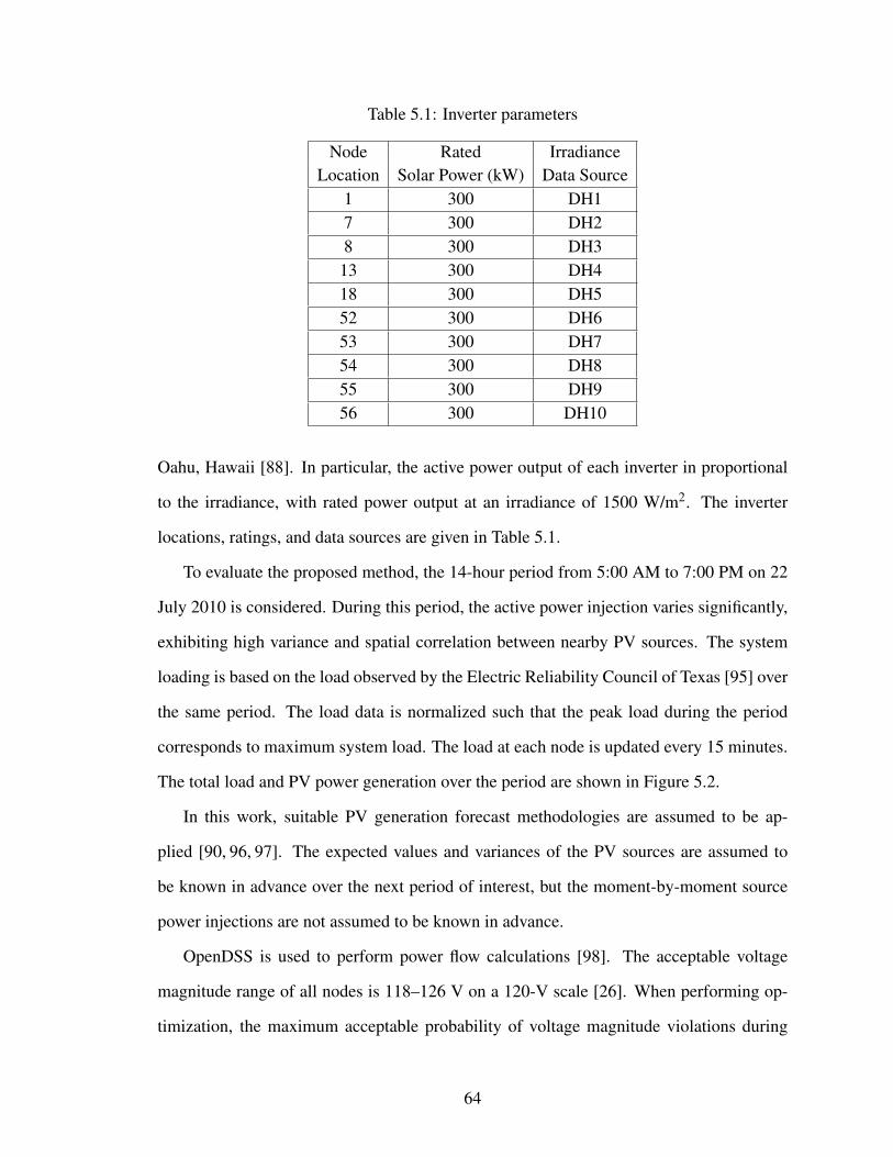
Table 5.1: Inverter parameters

Node Rated IrradianceLocation Solar Power (kW) Data Source

1 300 DH17 300 DH28 300 DH3

13 300 DH418 300 DH552 300 DH653 300 DH754 300 DH855 300 DH956 300 DH10

Oahu, Hawaii [88]. In particular, the active power output of each inverter in proportional

to the irradiance, with rated power output at an irradiance of 1500 W/m2. The inverter

locations, ratings, and data sources are given in Table 5.1.

To evaluate the proposed method, the 14-hour period from 5:00 AM to 7:00 PM on 22

July 2010 is considered. During this period, the active power injection varies significantly,

exhibiting high variance and spatial correlation between nearby PV sources. The system

loading is based on the load observed by the Electric Reliability Council of Texas [95] over

the same period. The load data is normalized such that the peak load during the period

corresponds to maximum system load. The load at each node is updated every 15 minutes.

The total load and PV power generation over the period are shown in Figure 5.2.

In this work, suitable PV generation forecast methodologies are assumed to be ap-

plied [90, 96, 97]. The expected values and variances of the PV sources are assumed to

be known in advance over the next period of interest, but the moment-by-moment source

power injections are not assumed to be known in advance.

OpenDSS is used to perform power flow calculations [98]. The acceptable voltage

magnitude range of all nodes is 118–126 V on a 120-V scale [26]. When performing op-

timization, the maximum acceptable probability of voltage magnitude violations during

64

Figure 5.2: Load profile and PV active power injection.

the optimization interval pmax of 5% is used. When assessing the results, the range of ac-

ceptable voltage magnitudes is slightly expanded to 117.95–126.05 V to avoid penalizing

methods for extremely small deviations (e.g., due to non-linearity, non-normal distribu-

tions, and correlation between sources).

All of the optimization problems are solved using an open-source linear programming

solver (Coin-OR Linear Programming) and an open-source quadratic programming solver

(Object Orientated Quadratic Programming). A workstation with an Intel Core i7-3770

processor operating at 3.40 GHz with 8 GB of memory was used to perform the results and

simulations. To control the convergence of the algorithm, the values δ = 0.8 and ε = 10−4

are used herein. The average time required to find ααα , βββ , and K for each 15-minute interval

over the entire 14-hour period is recorded as 180 seconds for the IEEE 123-node radial

distribution test feeder, which is significantly smaller than the 15-minute cycle time.

In order to examine the proposed method, three versions of three different methods

are considered. The three versions of these methods vary based on which variables are

considered. In the first version (V1), only the voltage regulator tap settings K are adjusted,

and the fixed and variable reactive power output of the PV inverters are zero (i.e., ααα = βββ =

0). This version is similar to conventional volt-var control methods in which only utility

equipment is controlled [99]. In the second version (V2), the voltage regulator tap settings

65

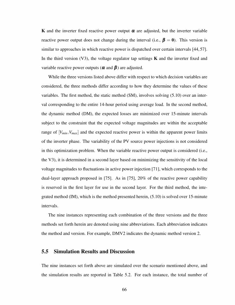
K and the inverter fixed reactive power output ααα are adjusted, but the inverter variable

reactive power output does not change during the interval (i.e., βββ = 0). This version is

similar to approaches in which reactive power is dispatched over certain intervals [44, 57].

In the third version (V3), the voltage regulator tap settings K and the inverter fixed and

variable reactive power outputs (ααα and βββ ) are adjusted.

While the three versions listed above differ with respect to which decision variables are

considered, the three methods differ according to how they determine the values of these

variables. The first method, the static method (SM), involves solving (5.10) over an inter-

val corresponding to the entire 14-hour period using average load. In the second method,

the dynamic method (DM), the expected losses are minimized over 15-minute intervals

subject to the constraint that the expected voltage magnitudes are within the acceptable

range of [Vmin,Vmax] and the expected reactive power is within the apparent power limits

of the inverter phase. The variability of the PV source power injections is not considered

in this optimization problem. When the variable reactive power output is considered (i.e.,

the V3), it is determined in a second layer based on minimizing the sensitivity of the local

voltage magnitudes to fluctuations in active power injection [71], which corresponds to the

dual-layer approach proposed in [75]. As in [75], 20% of the reactive power capability

is reserved in the first layer for use in the second layer. For the third method, the inte-

grated method (IM), which is the method presented herein, (5.10) is solved over 15-minute

intervals.

The nine instances representing each combination of the three versions and the three

methods set forth herein are denoted using nine abbreviations. Each abbreviation indicates

the method and version. For example, DMV2 indicates the dynamic method version 2.


The nine instances set forth above are simulated over the scenario mentioned above, and

the simulation results are reported in Table 5.2. For each instance, the total number of

66

Table 5.2: Simulation Results for All Instances

Violated Violation Violation Mean Worst-case Worst-casenode time percentage loss 15-min violation violated

Instance phases (s) (%) (kW) percentage (%) node phaseSMV1 88 20731 41 45.86 — —SMV2 72 23860 47 41.98 — —SMV3 114 43200 54 42.83 — —DMV1 43 5266 4.7 44.82 55 104 c-phaseDMV2 24 3629 3.4 40.90 43 104 c-phaseDMV3 0 0 0 41.10 0 —IMV1 18 1077 1.2 44.82 23 114 a-phaseIMV2 13 922 0.86 40.88 30 114 a-phaseIMV3 0 0 0 40.81 0 —

violated node phases (i.e., nodes with phase voltage magnitudes outside of the acceptable

range) is recorded. Also, the total time in which any violation is experienced in the sys-

tem is observed. For each node phase, two voltage violation percentages are calculated:

one for voltage magnitude over the acceptable limit, and the other for voltage magnitude

under the acceptable limit, corresponding to the constraints in (5.10). The largest of these

violation percentages across the system is presented. Mean loss is determined using power

calculated every second over the 14-hour period. The DM and IM both operate on a 15-

minute interval, so worst-case violations in any 15-minute interval are also considered for

these methods. The worst-case violation percentage is the violation percentage during the

worst 15-minute interval for a given instance. The node phase experiencing this worst-case

violation is also recorded.

As seen in Table 5.2, the SM results in many phases having voltage magnitude vio-

lations and the system experiencing such violations for a large fraction of the considered

interval. Even using the chance constraints in (5.10), the violation percentages are very

large with all versions. This occurs because this method does not account for any changes

over the day. In particular, it does not consider how load varies, including how it is corre-

67

lated over longer periods of time with the PV generation, which is shown in Figure 5.3 (a).

It can be seen that because of variations in loading, voltage magnitudes drift outside of the

acceptable range for large periods of time. However, it can also be seen that using variable

reactive power (i.e., V3), the voltage magnitudes are smoother. The SMV1 is a basic base-

line, but it is not particularly realistic because it does not correspond to how such systems

are ordinarily operated (e.g., tap changes by voltage regulators).

DMV1 is a more realistic baseline, with its behavior more closely representing dis-

tribution system volt-var control. It adjusts the tap settings each 15 minutes to minimize

system losses while maintaining expected voltage magnitudes within acceptable limits. It

can be seen in Table 5.2 that it is generally successful with reducing the overall violation

percentage, but it does experience 15-minute intervals in which it is not able to control

the voltage magnitudes effectively. Even DMV2, which uses fixed reactive power output

in each 15-minute interval cannot prevent the system from experiencing unacceptable 15-

minute intervals. This can be seen in Figure 5.3 (b). It can also be seen that using the

reactive power capability of the PV inverters results in smoother voltage magnitudes com-

pared with using tap changes alone. It can be seen in Table 5.2, that the DM versions are

more effective at reducing both voltage magnitude violations and losses than the analo-

gous SM versions. This is expected because the DM is making decisions every 15 minutes

compared with a single decision being made by the SM.

The proposed IM versions are also shown in Table 5.2. The IM versions also make a de-

cision every 15 minutes, but they formulate voltage magnitude limits as chance constraints.

It can be seen that they are more capable than the analogous DM versions at reducing both

voltage magnitude violations and losses. Figure 5.3 (c) indicates that IMV1 and IMV2 both

maintain voltage magnitudes in most intervals, but that the system still experiences unac-

ceptable 15-minute intervals because the violation percentage is larger than pmax = 5%.

From Table 5.2, the severity of these intervals for the IM versions is less than that of the

DM versions. Another observation that can be made from these results is that the worst-

68

Figure 5.3: (a) Node 114 a-phase voltage magnitude for SM, (b) Node 104 c-phase voltagemagnitude for DMV1 and DMV2, (c) Node 114 a-phase voltage magnitude for IMV1 andIMV2, and (d) Node 104 c-phase voltage magnitude for DMV3 and IMV3.

69

Figure 5.4: Losses for DMV1 and IMV3.

case 15-minute violation percentages for these instances should be less than approximately

pmax = 5%. A potential explanation for this discrepancy is that variable reactive power

injection (i.e., βββ ) is not used in IMV1 or IMV2.

The DMV3 seeks to keep the voltage magnitude within acceptable limits as shown in

Figure 5.3 (d) with no violation over the interval of interest and with successful reduction

in mean losses of 8.30% with respect to DMV1 as can be seen in Table 5.2. In DMV3, the

first layer is used to minimize the system loss, reserving some of the PV reactive power

capability for use in the second layer but not coordinating with the second layer. Conse-

quently, the DMV3 is somewhat conservative with respect to loss minimization (because

of the reserved capability) and results in less smooth voltages (because of the lack of coor-

dination). Alternatively, the IMV3 is formulated as an integrated control method in which

the use of inverter reactive power capability with the operation of voltage regulators is co-

ordinated to control voltage magnitude violations and reduce losses. It also exhibits no

voltage violations over the interval of interest, is able to further reduce losses (8.97% with

respect to DMV1 as shown in Figure 5.4 or an additional 8.07% reduction with respect to

the reduction obtained with DMV3), and results in smoother voltage magnitudes than other

instances as shown in Figure 5.3 (d).

The proposed IMV3 coordinates the actions of the distribution system equipment (e.g.,

70

Figure 5.5: (a) Tap positions for the voltage regulator connected to Node 160 for IMV3,(b) PV inverter three-phase reactive power injection at Node 55, and (c) and (d) the PVinverter three-phase fixed and variable reactive power injection (ααα and βββ ) at Node 55 forIMV3.

71

Table 5.3: The tap change operations of DM and IM versions over the interval of interest

Voltage Instanceregulators (V.R) Phase DMV1 DMV2 DMV3 IMV1 IMV2 IMV3V.R150−149 abc 2 2 3 2 5 1V.R9−14 a 3 3 6 7 2 1

V.R25−26a 4 6 6 8 5 5c 5 1 4 5 2 3

V.R160−67

a 7 9 14 7 5 11b 6 4 8 8 2 4c 7 3 11 11 6 6

Total number of tap changes 34 28 52 48 27 31

voltage regulators) with those of the PV inverters. Too frequently occurring tap change

operations is a maintenance concern for distribution system operators. While it is not

an explicit goal of the proposed method, it can help reduce tap change operations. The

control strategy used herein adjusts the voltage regulators infrequently (i.e., at most every

15 minutes over the 14-hour period) and the solution method in Figure 5.1 begins its search

for each interval from the solution for the previous interval. To study the effectiveness of

the IMV3 in terms of tap change operation reduction, the tap changing operations of the

IM and DM versions over the 14-hour period are shown in Table 5.3. Also, the tap settings

of one of the voltage regulators using IMV3 are shown in Figure 5.5 (a). It can be seen that

the tap settings are adjusted relatively infrequently during the course of the day in order to

improve losses and maintain voltages in response to changing load and PV injections. As

a result, IMV3 has fewer tap change operations in comparison with DMV3, which is the

instance with the most comparable performance. The proposed method is able to function

in this way because it uses variable PV reactive power injections to compensate for rapid

changes. The three-phase reactive power output of one of the PV inverters and its control

parameters (ααα and βββ ) are shown in Figure 5.5 (b),(c), and (d). It can be seen that whenever

the PV generation has a significant fluctuation as shown in Figure 5.2, PV inverters provide

or consume reactive power based on the PV generation patterns. The proposed method is

72

Table 5.4: Accuracy of the proposed method (i.e., optimal solutions)

15-minute Mean loss (kW) of the IMV3 Mean loss (kW) of the IMV3interval using MINLP using the proposed algorithm

5:00 AM to 5:15 AM 25.085 25.17:30 AM to 7:45 AM 19.547 19.548

10:00 AM to 10:15 AM 23.454 23.45410:30 AM to 10:45 AM 31.603 31.603

3:00 PM to 3:15 PM 53.622 53.623

Table 5.5: The sensitivity of the proposed method (i.e., initial solutions)

15-minute Mean loss (kW) of the IMV3 Mean loss (kW) of the IMV3interval using MINLP using the proposed algorithm

5:00 AM to 5:15 AM 26.351 25.1847:30 AM to 7:45 AM 20.782 19.553

10:00 AM to 10:15 AM 28 23.54510:30 AM to 10:45 AM 37.16 32.03

3:00 PM to 3:15 PM 60.215 53.68

able to minimize losses and maintain system voltages more effectively by coordinating the

response of the distribution system equipment with that of the PV inverters.

Because the proposed method is a supervisory control method targeting the perfor-

mance of the entire system, the most effective means of validating its performance is with

system studies. In this case, a widely available and acceptable test system (i.e., the IEEE

123-node test feeder from the IEEE PES Distribution System Analysis Subcommittee) is

used to validate the method. To validate the accuracy of the proposed method to find

the optimal solution for the control parameters, the mixed-integer nonlinear programming

(MINLP) solver is used to solve the proposed problem directly. The results show that the

proposed method matches the results obtained from the MINLP solver (within the toler-

ances used by the method) with much less computational time. For example, the five 15-

minute intervals have been randomly chosen from the interval of interest, and it is assumed

that the MINLP uses the optimal solutions of the proposed method as initial solutions. The

73

Table 5.6: Performance of IM


Method phases (s) (%) (kW) percentage(%) node phase

IMV1Expected – – 0.18 44.63 0.62 114 a-phaseSynthetic 4 13 0.2 44.66 0.66 114 a-phaseActual 18 1077 1.2 44.82 23 114 a-phase

IMV2Expected – – 0.07 40.70 2.04 114 a-phaseSynthetic 3 34 0.04 40.73 2.0 114 a-phaseActual 13 922 0.86 40.88 30 114 a-phase

IMV3Expected – – 0 40.60 0 —Synthetic 0 0 0 40.63 0 —Actual 0 0 0 40.81 0 —

results shown in Table 5.4 clearly indicate that optimal solutions of the proposed method

are very close to optimal solutions obtained by the MINLP. To better understand the perfor-

mance of the proposed method and the MINLP in terms of initial solutions, it is assumed

that the proposed method and the MINLP have the same initial solutions (i.e., zero initial

solutions). As can be seen in Table 5.5, the MINLP solver is far more sensitive to the

initial solution than the proposed method. This is expected because this type of problem

might mostly be non-convex with several local minima that are suboptimal solutions to

non-convex problems.

5.5.1 Sensitivity to Distribution Assumptions

The sensitivity of the IM is evaluated with respect to assumptions (i.e., the normality and

independence of the PV source powers). Statistical tests (e.g., the Anderson-Darling nor-

mality and Pearson correlation coefficient test) are used to measure both the normality of

the irradiance during the interval of interest and the linear correlation of PV sources. These

tests reject the hypothesis in which the irradiance during the interval of interest is normally

distributed and indicate a strong linear correlation between PV sources. In order to assess

the degree to which the proposed method fails to satisfy the assumptions, synthetic PV

74

Figure 5.6: (a) Node 114 a-phase voltage magnitude for synthetic and actual case of theIMV1, (b) Node 114 a-phase voltage magnitude for synthetic and actual case of the IMV2,and (c) Node 114 a-phase voltage magnitude for for synthetic and actual case of the IMV3.

75

source powers are constructed that have the same statistical characteristics (i.e., mean val-

ues and variances) as those in the actual PV source powers. However, the synthetic values

are constructed to be independent and normally distributed. It is possible to compare the

expected values (considered when computing the IM solution) to the simulation perfor-

mances of the IM in both the synthetic and the actual PV source powers. Table 5.6 for the

actual case indicates that the assumptions actually hold for the PV sources in the IMV1

and IMV2 (i.e., a maximum acceptable probability of voltage magnitude violation pmax of

5% at every 15-min), and do not hold with acceptable performance of the IMV3 because

of the variable PV reactive power output [85]. From Table 5.6, the IMV1 and IMV2 in the

synthetic case result in less node phases having voltage magnitude violations at some point

during the case and a lower period of time in which at least one node phase experiences

an unacceptable voltage magnitude. Another observation that can be made from Table 5.6

is that the IMV3 in both the synthetic and actual case results in no node phases having

voltage magnitude violations. In terms of the violation percentage, the IM versions in the

synthetic case more carefully seek to match the expected violation percentage. This is ex-

pected because the IM versions in the synthetic case more carefully match the assumptions

upon which the expected value is calculated. The lower value during the IM versions in the

synthetic case indicates improved voltage quality, but it also represents a more conservative

solution to the optimization problem because pmax is 5%. When compared with the actual

case, the IMV1 and IMV2 are less accurate to match the expected violation percentage

while the IMV3 matches the expected violation percentage. In terms of the mean loss, the

IMV1, IMV2, and IMV3 in the synthetic case carefully seek to match the expected value of

the mean loss, but in the actual case are relatively worse. In terms of the worst-case 15-min

violation percentage, the IMV1, IMV2, and IMV3 in the synthetic case are relatively close

to matching the expected value, but the IMV1 and IMV2 in the actual case fail to satisfy

the the assumption herein (i.e., a maximum acceptable probability of voltage magnitude

violation pmax of 5% at every 15-min) because these methods are highly sensitive to the

76

assumptions (i.e., the normality and independence of the PV source powers) without con-

sidering the variable PV reactive power output used to mitigate the variation of PV source

powers. When taken together, the results indicate that the IMV3 is not highly sensitive to

the assumptions regarding the normality and independence of the PV source powers.

The resulting voltage magnitude at the a phase of Node 114 is shown as an example in

Figure 5.6 for the synthetic and actual case. Figure 5.6 (a) and (b) indicate that the voltage

magnitude of the IMV1 and the IMV2 using the synthetic case has a shorter excursion

under the acceptable lower limit (117.95 V) than in the actual case. Figure 5.6 (c) also

indicates that the voltage magnitude of the IMV3 in both the synthetic and actual case does

not draft outside the acceptable ranges because it is not highly sensitive to the assumptions

used in this work, and exhibits a smoother voltage magnitude than the IMV1 and the IMV2

over the interval of interest because of the use of the variable PV reactive power output.

5.6 Conclusion

An integrated control method, formulated as a mixed-integer, nonlinear, chance-constrained

optimization problem, is presented to minimize the expected value of a figure of merit

while constraining the probability of unacceptable voltage magnitudes and considering the

uncertainty of PV power injections over the interval of interest. The integrated control

method combines the capabilities of distribution system equipment with the reactive power

capabilities of PV inverters to minimize system losses and constrain the probability of volt-

age violations. The proposed method uses suitable PV generation forecast methodologies

that include the expected values and variances of the PV sources, but not the moment-

by-moment values. The sensitivity of the proposed method IMV3 to the distribution as-

sumptions is considered, and it is found that the method is not highly sensitive to these

assumptions. The performance of the proposed method is evaluated using the IEEE 123-

node radial distribution test feeder under changing load and irradiance conditions, and it is

compared against two different existing methods. The results showed the capability of the

77

proposed method to minimize the system losses and mitigate voltage fluctuations.

78

Chapter 6

Coordination of PV Inverters and Volt-

age Regulators Considering Generation

Correlation and Voltage Quality Constr-

aints for Loss Minimization

6.1 Introduction

In this chapter, a coordinated volt-var control method is proposed to achieve the optimal

expected performance (i.e., system losses and voltage profiles), while considering spatial

correlations among the DGs. It also seeks to maintain voltage magnitudes within an accept-

able range, by formulating chance constraints on the voltage magnitude and considering

the uncertainty of DG power injections, over the interval of interest. Although the volt-var

control proposed herein uses infrequent communication between the distribution system

operator and voltage regulator settings, it can respond successfully to a rapid change in

irradiance conditions, by using DG control parameters. Thus, allowing them to respond

to such changes in real time. The control strategy is formulated as a mixed-integer, non-

linear, chance-constrained optimization problem, and a heuristic approach, using power

79

flow solutions and linearization to find optimal solutions. The proposed method is based

on previous work [85], where this method only used the reactive power output of DGs to

improve the system performance, and to previous work [93], where this method used distri-

bution system equipment including PV inverters, to improve the system performance. The

main improvements of this work are: a consideration of the spatial correlation among DGs,

improved voltage magnitude profiles by limiting the variation of voltage magnitudes, eval-

uation of the system performance over longer periods, and a more thorough comparison

with existing methods to achieve a reasonable benchmark for comparison.

Despite the fact that the proposed method mainly targets the improvement of the system

performance (i.e., the system losses and voltage magnitude profiles), a frequent operation

of voltage regulators can be indirectly remedied using an effective approach. This approach

involves reducing the number of possible interactions between DGs and voltage regulators.

This can be achieved by adjusting the voltage regulators every 15 minutes, over the 14-hour

period, and restarting the proposed solution algorithm from a previous optimal solution.

The DG source powers are distributed near each other in this work. Therefore, the

DG source powers are highly correlated with each other, based on statistical tests used to

measure the normality of irradiance during this interval and the linear correlation of DG

sources. Consequently, the impact of spatial correlations among DG source powers on the

accuracy of the proposed method and the voltage profile enhancement is mainly studied

in this chapter. The proposed method is validated using an IEEE 123-node radial distribu-

tion system. The results showed that the proposed method is promising for improving the

system performance and voltage magnitude profile with intermittent renewable resources.

The remainder of this chapter is described as follows. Section 6.2 presents the system

description and approximation for the figure of merit and the system voltage magnitudes.

The problem formulation is provided in Section 6.3. Section 6.4 describes the test system

description based on the IEEE 123-node radial distribution test feeder [87]. Simulation

results and discussion are explored in Section 6.5. Finally, conclusions are given in Sec-

80

tion 6.6.


A coordinated volt-var control method using the PV inverters and voltage regulators is

presented herein to minimize the expected value of a figure of merit U and mitigate the

voltage magnitude fluctuations, while considering the spatial correlation among DGs and

constraining the probability of unacceptable voltage magnitudes in the distribution sys-

tems. The strategy used herein is based on solving nonlinear problems using power flow

solutions and approximations derived from power flow solutions in a heuristic method. The

equations that explain the system description and approximation for the figure of merit and

the system voltage magnitudes mentioned in 5.2 will be used in this section.


The proposed method is formulated as a nonlinear, mixed-integer, chance-constrained

problem with predefined probabilistic constraints. The proposed method seeks to improve

the expected value of a figure of merit including optimal expected inverter control param-

eters and voltage regulator settings, while ensuring that the probability of unacceptable

81

voltage magnitudes over the interval of interest is satisfied1:

minααα,βββ ,K E [U ]


∀i ∈ {1,2, . . . ,Nnode} Pr[|Vi| ≥Vmax]≤ pmax

000≤ (Var[|V|])◦ 12 ≤ σσσmax

(E[Pinv]◦2 +E[Qinv]

◦2)◦12 ≤ Smax



Kmin ≤K≤Kmax,

(6.1)

where Vi is the voltage at node phase i, pmax is the maximum acceptable probability for a

node phase voltage magnitude to exceed Vmax or to fall below Vmin, σσσmax = σmax1Nnode×1 is

the vector of the maximum expected standard deviation of the voltage magnitudes, Smax ∈

RNinv×1 is a vector of the apparent power limits of the inverter phases, αααmin, βββ min, αααmax,

βββ max are minimal and maximal allowable inverter control parameters, and Kmin and Kmax

are minimal and maximal allowable voltage regulator tap settings.

It is assumed that the expected value and the variance of each source power, i.e.,

E[Psource] and Var[Psource], are known over the interval of interest. This nonlinear prob-

lem is solved iteratively, and is solved based on a linearization about the previous solution

estimate (i.e., ααα0, βββ 0, and K0).

It is possible to approximate E[U ] using (5.8):

E[U ]≈U0 +UTP(HE[Psource]−Pinv0)−UT

QQinv0−UTKK0

+UTQααα +UT

Q diag[HE[Psource]]βββ +UTKK


ββββ + cT

KK, (6.2)

1E is the expectation operator

82

where

c0 =U0 +UTP(HE[Psource]−Pinv0)−UT

QQinv0−UTKK0 (6.3)

cα = UQ (6.4)

cβ = diag[HE[Psource]]UQ (6.5)

cK = UK . (6.6)


(5.9) as

E[|V|]≈ V0 +VP(HE[Psource]−Pinv0)−VQQinv0−VKK0

+VQααα +VQ diag[HE[Psource]]βββ +VKK

= N0 +Nαααα +Nβ βββ +NKK, (6.7)

where

N0 = V0 +VP(HE[Psource]−Pinv0)−VQQinv0−VKK0 (6.8)

Nα = VQ (6.9)

Nβ = VQ diag[HE[Psource]] (6.10)

NK = VK . (6.11)

In order to explore the influence of the spatial correlation among the PV source powers,

the covariance matrix among the PV source powers is considered when expressing the

variance of the voltage magnitudes [100]. Accordingly, the source powers are assumed

to be distributed dependently over the interval of interest, and the variance of the voltage

magnitudes can be expressed from (5.9) as2

Var[|V|]≈ (VPH+VQ diag(βββ )H)Cov[Psource](VPH+VQ diag(βββ )H)T, (6.12)

where Cov[Psource] is the covariance matrix among PV source powers, and the standard

deviation can be written as2Cov is the covariance operator.

83

(Var[|V|])◦12 ≈ ((((VPH+VQ diag[βββ ]H)Cov[Psource](VPH+VQ diag[βββ ]H)T)◦ INnode)

◦1Nnode×1)◦ 1

2 . (6.13)



(Var[|V|])◦12 ≈ ((((VPH+VQ diag[βββ 0]H)Cov[Psource](VPH+VQ diag[βββ ]H)T)◦ INnode)

◦1Nnode×1)◦ 1

2 +12((VPHCov[Psource]HT ◦VQ +(HCov[Psource]HTVT

P)T ◦VQ

+(HCov[Psource]HT(VQ diag[βββ 0])T)T2◦VQ)◦ ((((((VPH+VQ diag[βββ 0]H)

·Cov[Psource](VPH+VQ diag[βββ 0]H)T)◦ INnode)◦1Nnode×1)◦ 1

2 11×Ninv)◦(−1)))

· (βββ −βββ 0)

= M0 +Mβ βββ , (6.14)

where

M0 = ((((VPH+VQ diag[βββ 0]H)Cov[Psource](VPH+VQ diag[βββ ]H)T)◦ INnode)◦1Nnode×1)◦ 1

2

− 12((VPHCov[Psource]HT ◦VQ +(HCov[Psource]HTVT

P)T ◦VQ +(HCov[Psource]HT

· (VQ diag[βββ 0])T)T2◦VQ)◦ ((((((VPH+VQ diag[βββ 0]H)Cov[Psource](VPH+VQ

·diag[βββ 0]H)T)◦ INnode)◦1Nnode×1)◦ 1

2 11×Ninv)◦(−1))βββ 0 (6.15)

Mβ =12((VPHCov[Psource]HT ◦VQ +(HCov[Psource]HTVT

P)T ◦VQ +(HCov[Psource]HT

· (VQ diag[βββ 0])T)T2◦VQ)◦ ((((((VPH+VQ diag[βββ 0]H)Cov[Psource](VPH+VQ

·diag[βββ 0]H)T)◦ INnode)◦1Nnode×1)◦ 1

2 11×Ninv)◦(−1))) (6.16)




Pr[|Vi| ≤Vmax]≥ 1− pmax, (6.18)

84

can be expressed as

Φ

(Vmin−E[|Vi|]√

Var[|Vi|]

)≤ pmax (6.19)

Φ

(Vmax−E[|Vi|]√

Var[|Vi|]

)≥ 1− pmax, (6.20)


substitution of (6.7) and (6.14), these constraints ∀i ∈ {1,2, . . . ,Nnode} can be expressed as

Vmin− (N0 +Nαααα +Nβ βββ +NKK)≤Φ−1(pmax)(M0 +Mβ βββ ), (6.21)

Vmax− (N0 +Nαααα +Nβ βββ +NKK)≥Φ−1(1− pmax)(M0 +Mβ βββ ), (6.22)


valid for βββ sufficiently close to βββ 0. Specifically, an additional constraint is introduced to

ensure that the approximate standard deviation is non negative:

000≤M0 +Mβ βββ ≤ σσσmax, (6.23)

The maximum expected reactive power being injected by each inverter phase is limited by

the apparent power limits of the inverter phase:

−(S◦2max−P◦2inv0)◦ 1

2 ≤ (ααα +βββ ◦Pinv0)≤ (S◦2max−P◦2inv0)◦ 1

2 , (6.24)

By combining (6.2) and (6.21)–(6.24), the solution to the optimization problem in (6.1) can

be approximated by the solution of a linear programming problem of the form

minx cTx

subject to Ax≤ b

xmin ≤ x≤ xmax,

(6.25)

where x = [αααT βββT KT]T, c = [cT

α cTβ

cTK]

T, and

85

A =

−Nα −(Nβ +Φ−1(pmax)Mβ ) −NK

Nα Nβ +Φ−1(1− pmax)Mβ −NK

03Nnode×Ninv −Mβ 03Nnode×Nt

03Nnode×Ninv Mβ 03Nnode×Nt

INinv diag[Pinv0] 0Ninv×Nt

−INinv −diag[Pinv0] 0Ninv×Nt

b =



M0

σσσmax−M0


2


2

,

where 0m×n is the m×n matrix filled with zero. The algorithm that describes the scenario

of finding optimal solutions for the optimization problem given in (6.1) is mentioned in

5.3.


To examine the performance of the proposed volt-var control, six methods, based on un-

balanced three-phase distribution test system, are studied, by using the modified IEEE

123-node radial distribution test feeder [87]. The test feeder is described in Figure 3.2.

This test system used herein has a nominal voltage of 4.16 kV and consists of 123 nodes. It

also has unbalanced loads, and four voltage regulators for voltage control between Nodes

150 and 149, 9 and 14, 25 and 26, and 160 and 67. In this study, ten three-phase four

wire PV inverters are connected to nodes 1, 7, 8, 13, 18, 52, 53, 54, 55, and 56. Their

86

locations are based on a previous study [71] that showed inverters situated in these loca-

tions with spatially correlated irradiance can cause significant voltage fluctuations. The PV

inverters injected at specified nodes can adjust the fixed and variable reactive power output

for each phase independently. The rated solar power of all PV inverters is 300 kW. For

the power generation of these PV inverters, one-second global horizontal irradiance data

collected by the National Renewable Energy Laboratory Solar Measurement Grid in Oahu,

Hawaii is used herein [88]. The solar irradiance data sources are measured based on ten

irradiance sensors placed in different locations (e.g., DH1–DH10). In particular, the active

power output of each inverter is proportional to the irradiance with rated power output at

an irradiance of 1500 W/m2. For the study proposed herein, irradiance data from 5:00 AM

to 7:00 PM on 22 July 2010 is used. During this period, the active power injection varies

significantly, exhibiting high variance and spatial correlation between nearby PV sources.

The system loading is based on the load observed by the Electric Reliability Council of

Texas [95] over the same period. The load data is normalized such that the peak load dur-

ing the period corresponds to maximum system load. The load at each node is updated

every 15 minutes. The total load and PV power generation are illustrated in Figure 5.2 for

a 14-hour period. In this study, suitable PV generation forecast methodologies are assumed

to be applied [90,96,97]. The expected values and variances of the PV sources are assumed

to be known in advance over the next period of interest, but the moment-by-moment source

power injections are not assumed to be known in advance.

OpenDSS is used to perform power flow calculations [98]. The voltage magnitude

limits of all nodes are assumed to be 118–126 V on a base of a 120-V scale [26]. When

performing optimization, the maximum acceptable probability of voltage magnitude viola-

tions during the optimization interval pmax of 5% is used. When assessing the results, the

range of acceptable voltage magnitudes is slightly expanded to 117.9995–126.0005 V to

avoid penalizing methods for extremely small deviations (e.g., due to non-normal distribu-

tions).

87

In order to examine the proposed method, six different methods are considered. In

first method, the baseline method (BM), the voltage regulator tap settings K are only ad-

justed, and the fixed and variable reactive power output of the PV inverters are zero (i.e.,

ααα = βββ = 0). In this optimization problem, the tap settings are adjusted every 15 minutes

to minimize system losses while maintaining expected voltage magnitudes within accept-

able limits, and the variability of the PV source power output injections is not considered.

For the rest of the methods, the voltage regulator tap settings K and the inverter fixed and

variable reactive power outputs (ααα and βββ ) are adjusted every 15 minutes. In the second

method, the dynamic method (DM), the expected losses are minimized over 15-minute in-

tervals subject to the constraint that the expected voltage magnitudes are within the accept-

able range of [Vmin,Vmax] and the maximum expected reactive power is within the apparent

power limits of the inverter phase. The variability of the PV source power injections is

not considered in this optimization problem. When the variable reactive power output is

considered, it is determined in a second layer based on minimizing the sensitivity of the

local voltage magnitudes to fluctuations in active power injection [71], which corresponds

to the dual-layer approach proposed in [75]. As in [75], 20% of the reactive power capa-

bility is reserved in the first layer for use in the second layer. For the third method, the

integrated method (IM), (6.1) is solved over 15-minute intervals with considering the vari-

ability of the PV source power injections. For the fourth method, the limited integrated

method (LIM), (6.1) is solved over 15-minute intervals, by considering the variability of

the PV source power injections and limiting the variation of voltage magnitudes. For the

fifth method, the correlated integrated method (CIM),which is the method presented herein,

(6.1) is solved over 15-minute intervals, by considering the spatial correlations among the

PV source powers. For the sixth method, the limited correlated integrated method (LCIM),

(6.1) is solved over 15-minute intervals, by considering the spatial correlations among the

PV source powers and limiting the variation of voltage magnitudes.

88


The six methods are simulated over the scenario mentioned above, and the simulation re-

sults are reported in Table 6.1. For each method, the total number of violated node phases

(i.e., nodes with phase voltage magnitudes outside of the acceptable range) is recorded.

Also, the total time in which any violation is experienced in the system is observed. For

each node phase, two voltage violation percentages are calculated: one for voltage mag-

nitude over the acceptable limit, and the other for voltage magnitude under the acceptable

limit. The largest of these violation percentages across the system is presented. Mean loss

is determined using power calculated every second over the 14-hour period. All meth-

ods operate on a 15-minute interval, so the worst-case violations in any 15-minute interval

are also considered for these methods. The worst-case violation percentage is the viola-

tion percentage during the worst 15-minute interval for a given method. The node phase

experiencing this worst-case violation is also recorded.

The voltage magnitude variation can be constrained based on the desirable standard

deviation of the voltage magnitudes in (6.23). This efficient constraint helps the proposed

method to match assumptions made in this work and mitigate the impact of non-normal

distributions on the proposed method. In order to evaluate the performance of the proposed

method in terms of the voltage magnitude variation, all methods are studied to understand

the performance of these methods on the distribution voltage magnitude variations. All

methods are compared with each other and evaluated on their performance based on several

metrics. The metrics are described as follows. The mean violation time is the average of

the violation time for all nodes experienced a voltage magnitude outside of the acceptable

limits during the case. The voltage magnitude violation indicates each node phase voltage

magnitude is over the acceptable limit, a certain fraction of the voltage magnitude during

the case, and under the acceptable limit, a certain fraction of the voltage magnitude. The

mean voltage magnitude violation is the mean of the aforementioned fraction. The largest

89

Table 6.1: Simulation results for all methods


method phases (s) (%) (kW) percentage (%) node phaseBM 49 8516 7 44.82 62 104 c-phaseDM 2 900 1.63 41.10 66 104 c-phaseIM 3 1683 2.47 40.81 32 114 a-phaseLIM 4 738 1.06 40.84 16.45 114 a-phaseCIM 5 515 0.47 40.82 8 114 a-phaseLCIM 1 60 0.12 40.83 4.4 114 a-phase

such fraction is the maximum voltage magnitude violation. The standard deviation of the

voltage magnitudes of Node i over the time interval m is used and defined below

σim =

√√√√ 1Tin

Tin

∑t=1

(|Vim(t)|− |V?im|)2, (6.26)

where |V?im| is the mean of the voltage magnitudes of Node i during the time interval m,

i ∈ {1,2, ...,Nnode}, t ∈ {1,2, ...,Tin} and Tin is the time interval, and m = {1,2, ...,M}

and M is the total number of the time interval over the interval of interest. The standard

deviation of the voltage magnitudes each time interval can be expressed as

σm =

√√√√ 1Nnode

Nnode

∑i=1

σ2im. (6.27)

The maximum standard deviation over the interval of interest is given by

maxm∈M

maxi∈{1,2,...,Nnode}

σim, (6.28)

where σim ∈RM+ is a standard deviation of the voltage magnitudes over the time interval m,

and the average standard deviation over the interval of interest is given by

1M

M

∑m=1

σm. (6.29)

As it can be seen in Table 6.1, the BM failed to maintain the overall violation percent-

ages within the acceptable range because the violation percentage is larger than pmax = 5%.

90

Also, the voltage magnitudes drift outside of the acceptable range for larger periods of time

than the other methods as seen in Figure 6.1 (a). Table 6.1 also shows that the DM is more

effective than the BM in reducing both voltage magnitude violations and system losses.

This is expected because the DM makes its decision every 15 minutes, but it uses the in-

verter fixed and variable reactive power outputs (ααα and βββ ) to improve system performance,

compared with a single decision being made by the BM (i.e., K). However, the DM is

somewhat conservative with respect to loss minimization because of the reserved capabil-

ity of PV inverters. The lack of coordination between the two layers in the DM causes the

voltage magnitudes to have unacceptable 15-minute intervals and be less smooth during

the interval of interest as shown in Figure 6.1 (b) compared with the LCIM.

The IM also makes its decision every 15 minutes and uses the inverter fixed and variable

reactive power outputs (ααα and βββ ) to improve system performance, but it formulates voltage

magnitude limits as chance constraints. From Table 6.1, the IM is obviously more capable

of reducing system losses, albeit the IM is less capable than the DM in reducing voltage

magnitude violations. This is expected because the IM formulates the voltage magnitude

limits as chance constraints to reduce system losses. In order to mitigate the impact of non-

normal distribution of irradiance data used herein, the variation of the voltage magnitudes is

limited in the IM (i.e., the LIM). Consequently, as noticed in Table 6.1, the performance of

the IM is relatively improved in terms of violation time, violation percentage, and the unac-

ceptable 15-minute interval. However, there is a trade off between limiting the variation of

the voltage magnitudes, which also restricts chance constraints, and reducing system losses

as noticed in Table 6.1. Another observation that can be made from Table 6.1 is that the IM

still experiences unacceptable 15-minute intervals due to non-linearity, non-normal distri-

butions, and the spatial correlations among PV sources. Consequently, the main advantage

obtained using the LIM is that, in addition to improving the system performance, the LIM

has less voltage magnitude variability than the IM in most of the interval of interest as seen

in Figure 6.1 (c).

91

The CIM is the method proposed herein in this chapter. It also makes its decision every

15 minutes and formulates voltage magnitude limits as chance constraints, but it considers

spatial correlations among the PV sources. The simulation results in Table 6.1 indicate

that the performance of the CIM to match assumptions is sufficiently higher than the afore-

mentioned methods. As seen in Table 6.1, the CIM results in a lower period of time in

which at least one node phase experiences an unacceptable voltage magnitude with more

reduction of the overall violation percentage. Table 6.1 also indicates that the severity of

the worst-case 15-minute violation percentages for the CIM is less than that of others, but it

still experiences unacceptable 15-minute intervals. This is expected because of non-normal

distribution of irradiance data. Although the CIM is also effective in reducing mean loss

with respect to the BM, the CIM still is somewhat more conservative with respect to loss

minimization than the IM (0.022% more). The LCIM is also shown in Table 6.1. In the

CIM, the variation of the voltage magnitudes is also limited to mitigate the impact of a

non-normal distribution of irradiance data (i.e., the LCIM). Therefore, as seen in Table 6.1,

the LCIM results in less node phase having voltage magnitude violations than the other

methods, and a lower period of time in which at least one node phase experiences an un-

acceptable voltage magnitude with also more reduction of the overall violation percentage.

Another observation that can be made from these results is that the worst-case 15-minute

violation percentage for the LCIM is less than pmax = 5%. The results also show that

the LCIM has slightly worse losses than the CIM (0.022% more with respect to the BM).

This is expected due to limiting the variability of the voltage magnitudes that somewhat

makes the LCIM conservative in loss reduction. The overall conclusion is that the simula-

tion results in Table 6.1 indicate that the performance improvement of the LCIM to match

assumptions has been observed in both voltage magnitude violations and the worst-case

15-minute violation percentage. Also, it can be noticed from Figure 6.1 (d) that the LCIM

has smoother voltage magnitudes than the CIM in most of the interval of interest.

The performance of all the methods during the interval of interest to mitigate a voltage

92

Figure 6.1: (a) Node 104 c-phase voltage magnitude for BM and LCIM, (b) Node 104 c-phase voltage magnitude for the DM and LCIM, (c) Node 114 a-phase voltage magnitudefor the IM and LIM, and (d) Node 114 a-phase voltage magnitude for the CIM and LCIM.

93

Table 6.2: Simulation results for voltage magnitude violations

Mean Mean Maximum Mean Maximumviolation violation violation standard standard

method time (s) (mV) (mV) deviation (mV) deviation (mV)BM 118 225×10−3 499 89.5 259.8DM 3.3 1.65×10−4 7.3 1.4 4.3IM 6.12 4.6×10−4 23.5 4.7 12.83LIM 2.68 8.1×10−5 7.15 1.67 3.92CIM 2.04 3.1×10−4 45 12.61 42.5LCIM 0.22 1.26×10−5 9.6 2.22 3.67

variation is shown in Table 6.2. In terms of mean violation time, the LCIM is successful in

reducing the overall mean violation time. Also, the Table 6.2 indicates that the LCIM has

the best improvement in a mean voltage magnitude violation. Furthermore, it matches the

desirable constraint of standard deviations of the voltage magnitudes during the interval of

interest (e.g., σmax = 3.5 mV on a base of 120-V scale chosen based on the best reduction in

the system loss and improvement in the voltage magnitude profile for the LCIM and LIM).

To study the behavior of the LCIM and LIM in this chapter further, the worst-case 15-

min standard deviation of voltage magnitude resulting at the a phase of Node 114 for CIM

and IM is shown as an example in Figure 6.2 compared with the LCIM and LIM. As seen in

Figure 6.2 (a) and (b) that without limiting the standard deviation of the voltage magnitude

over the interval of interest, the CIM and IM experience more observable voltage mag-

nitude variations than the LCIM and LIM. As a result, limiting the standard deviation of

the voltage magnitude over the interval of interest helps to mitigate the voltage magnitude

violation and improve the voltage magnitude profile of all system nodes.

The rapid fluctuation in PV output powers results in an excessive number of tap change

operations of voltage regulators. While the main goal of the proposed method is not to

reduce tap change operations, this efficient strategy used herein helps to reduce that. The

control strategy adjusts the voltage regulators infrequently (i.e., at most every 15 minutes

94

Figure 6.2: The worst 15-minute standard deviation of voltage magnitude of Node 114a-phase voltage magnitude for the CIM and LCIM in (a) and for the IM and LIM in (b).

over the 14-hour period) and the solution method in Figure 5.1 begins its search for each

interval from the solution for the previous interval. To study the effectiveness of the LCIM

in terms of a tap change operation reduction, the total number of tap changing operations

of all methods over the 14-hour period are shown in Table 6.3. Also, the tap settings of one

of the voltage regulators using the CIM and LCIM is shown in Figure 6.3. Figure 6.3 (b)

shows that constraining the voltage magnitude variations helps to adjust tap change opera-

tions relatively infrequently compared with Figure 6.3 (a) during the course of the day in

order to improve losses, enhance the voltage profiles, and maintain voltages in response to

changing load and PV injections. As a result, the LCIM has fewer tap change operations

in comparison with the other methods as shown in Table 6.3.

95

Figure 6.3: Tap positions for the voltage regulator connected to Node 160 for the CIM in(a) and for the LCIM in (b).

Table 6.3: Total number of tap change operations of all methods over the interval of interest

Voltage Methodregulators (V.R) Phase BM DM IM LIM CIM LCIMV.R150−149 abc 2 3 1 1 1 1V.R9−14 a 3 6 1 2 1 1

V.R25−26a 4 6 5 11 6 4c 5 4 3 3 2 2

V.R160−67

a 7 14 11 10 8 3b 6 8 4 4 8 2c 7 11 6 8 8 4

Total number of tap changes 34 52 31 39 34 17

96

6.6 Conclusion

A correlated integrated method that is formulated as a mixed-integer, nonlinear, chance-

constrained optimization problem is proposed to optimize the expected performance of a

distribution system. It optimizes this performance while considering the spatial correlation

among PV sources, maintaining acceptable system voltage magnitudes, and considering

the uncertainty of PV power injections. The proposed method uses both the PV inverter

capability to inject or absorb a reactive power and the voltage control equipment to min-

imize the system losses, mitigate voltage magnitude fluctuations, improve voltage mag-

nitude profiles, and indirectly reduce tap operations of voltage regulators. The proposed

method formulated the voltage magnitude requirements as chance constraints. The per-

formance is assessed using IEEE 123-node radial distribution test feeder under load and

irradiance changing, and more thoroughly by the consideration of longer periods of time

and comparison with existing methods. The final results demonstrated that the proposed

method can effectively improve the system performance of distribution systems with PV

sources.

97

Chapter 7

Conclusion and Future Work

7.1 Conclusion

In this dissertation, several volt-var control methods using voltage and reactive power con-

trol equipment are proposed to provide applicable solutions to mitigate the adverse effects

that DGs might have. In Chapter 3, a method of achieving optimal expected performance

while maintaining appropriate system voltage magnitudes is proposed. Specifically, this

technique is used to optimize only the reactive power output of DGs to improve expected

system performance (i.e., the operating profit) and to compensate for variations in active

power injections during an upcoming interval. Three different cases are studied to under-

stand the performance of the proposed method under various conditions (i.e., the cloudy

case, sunny case, and transient case). Each of these cases represents a 15-minute interval

over which the operation of traditional voltage regulation equipment (i.e., capacitor banks

and voltage regulators) is considered fixed. The proposed chance-constrained optimization

(CCO) method is examined against three other methods. The baseline method involves the

inverters only providing active power without any reactive power. The local voltage con-

trol (LVC) method involves using a volt-var control to maintain the system voltage mag-

nitudes within acceptable limits and coordinates the injecting or the absorbing of reactive

power among several distributed generators with a piecewise linear droop characteristic.

The global violation unbalanced (GVU) method is formulated to inject independent reac-

98

tive powers based on real power injections into each phase to mitigate voltage violations.

The CCO is compared to baseline, LVC, and GVU methods on the IEEE 123-node ra-

dial distribution feeder under various generation conditions. Three cases were considered,

corresponding to cloudy, sunny, and transient conditions. The results showed that in each

of these cases, the CCO method is able to improve the average operating profit over the

other methods while maintaining acceptable voltage magnitudes and reducing distribution

system losses. When performance of the proposed method is examined in terms of sensi-

tivity to the distribution assumptions made in this chapter, the results showed that the CCO

method is not highly sensitive to these assumptions.

In Chapter 4, the integrated chance-constrained optimization (ICCO) is proposed. The

ICCO combines the conventional voltage control equipment (e.g., voltage regulators) and

the capability of PV inverters to inject reactive power along with active power to maxi-

mize the expected value of a figure of merit (i.e., the operating profit) while constraining

the probability of unacceptable voltage magnitudes. The ICCO uses short-term forecasts

that include the expected mean and variance of the active power injection and expected

load and formulates the voltage magnitude requirements as chance constraints. The opti-

mal voltage regulator tap settings and PV inverter reactive parameters can be transmitted

periodically from a centralized control center (e.g., every 15 minutes) via local communi-

cation channels. The ICCO method is examined against three other methods. The baseline

method involves the PV inverters only providing active power without reactive power. The

CCO method seeks to find optimal expected performance with respect to a figure of merit

of interest while maintaining appropriate system voltage magnitudes without considering

the optimal voltage regulator tap settings. The dual global violation unbalanced (DGVU)

method involves calculating the optimal control settings in the first layer (e.g., voltage regu-

lation tap settings and reference reactive power of PV inverters), and they are kept constant

for the second layer. In the second layer, PV inverter reactive power is used to mitigate

voltage variations. The ICCO is compared to baseline, CCO, and DGVU methods on the

99

IEEE 123-node radial distribution feeder under various generation conditions. Using the

same three cases mentioned above, the results showed that the ICCO method was effec-

tive in both improving performance with respect to the figure of merit and constraining the

probability of voltage magnitude violations.

In Chapter 5, a supervisory volt-var control method focusing on system optimization is

proposed. The proposed method is addressing a figure of merit of interest to the distribution

system operator (e.g., system loss) while constraining the probability of unacceptable volt-

age magnitudes occurring during the interval of interest. The proposed method performs

this control by adjusting parameters associated with the fixed and variable reactive power

produced by the inverter and the voltage regulator tap settings, by formulating chance con-

straints on the voltage magnitudes. The proposed method includes an enhanced solution

algorithm to the mixed-integer problem that accounts for the discrete nature of voltage

regulator tap settings and accelerates the process of finding initial feasible points. The

performance of the proposed method is also evaluated more thoroughly by consideration

of longer periods of time, and, by comparison, with existing methods. Although the pro-

posed method does not explicitly seek to reduce the number of tap change operations, the

proposed control method uses an efficient approach to limit the number of tap change op-

erations indirectly. The strategy used herein helps the voltage regulators to be infrequently

adjusted (i.e., every 15 minutes over the 14-hour period) and proposes restarting the al-

gorithm from the previous solution, helping with reducing tap change operations as well.

This volt-var control strategy also requires both infrequent communication with the distri-

bution system operator and infrequent changes to voltage regulator settings. However, it

can respond to rapidly changing conditions by providing control parameters to the inverters

to allow them to respond to such changes in real time, a capability that is available in smart

inverters. In order to examine the proposed method, three different methods that control

the variable and fixed reactive power output of the DG inverters and the voltage regulator

tap settings are considered. These methods are mainly defined by static method, dynamic

100

method, and integrated method. Each of these methods involves three versions which vary

based on which variables are considered. The performance of the proposed method is

evaluated using the IEEE 123-node radial distribution test feeder under changing load and

irradiance conditions. To better understand the performance of the proposed method in

terms of sensitivity to the distribution assumptions made in this chapter after considering

the voltage regulator tap setting as a control variable, the sensitivity of the proposed method

to the distribution assumptions is considered. The results showed that the method is not

highly sensitive to these assumptions. The results also showed the effectiveness of the

proposed method to minimize the system losses and mitigate voltage fluctuations.

In Chapter 6, a coordinated control of voltage regulators and PV inverters considering

PV generation correlations to achieve the optimal expected performance is proposed. The

proposed method performs this integrated control by using existing PV inverters and the

voltage control equipment to improve the expected system performance while considering

the spatial correlation among PV source powers. Six different methods are studied to un-

derstand the performance of the proposed method under various conditions. In the baseline

method (BM), the voltage regulator tap settings are only adjusted every 15-minute period

while keeping the expected voltage magnitudes within acceptable ranges without consider-

ing the variability of the PV source power injections. The dynamic method (DM) involves

the fixed and variable PV inverter parameters and the voltage regulator tap settings are ad-

justed every 15-minute period while maintaining the expected voltage magnitudes within

acceptable limits without considering the variability of the PV source power injections.

The integrated method (IM) involves the fixed and variable reactive power output of PV

inverters and the voltage regulator tap settings are adjusted every 15-minute period while

maintaining the expected voltage magnitudes within acceptable limits, by formulating the

voltage magnitudes as chance constraints and considering the variability of the PV source

power injection. The limited integrated method (LIM) involves the IM used with constrain-

ing the expected variation of voltage magnitudes by a desirable standard deviation. The

101

correlated integrated method (CIM) involves the voltage regulator tap settings and the PV

inverter reactive power output parameters are adjusted every 15-minute period while main-

taining the expected voltage magnitudes within acceptable limits and considering the spa-

tial correlation among the PV source powers. In the limited correlated integrated method

(LCIM), the CIM is used with constraining the expected variation of voltage magnitudes

within a desirable standard deviation. The performance of the proposed method is assessed

using IEEE 123-node radial distribution test feeder under load and irradiance changing, and

compared with five methods for comparison purpose. The final results showed that the pro-

posed method is promising for improving the system performance and voltage magnitude

profile with intermittent renewable resources.

7.2 Future Work

For the volt-var control method discussed in Chapter 3, which only used the reactive power

outputs of PV inverters to optimize the system performance, the price for reactive power

injected is ignored when formulating the proposed method. In future work, the price for

reactive power injected by the PV inverter will be added to the figure of merit equation to

make the proposed method more realistic. The modified figure of merit will be expressed

as

U =Nload

∑i=1

CloadPload,i−Npv

∑i=1

CpvPpv,i−Npv

∑i=1

CqvQpv,i−Nin

∑i=1

CinPin,i, (7.1)

where Cqv is the price paid for reactive power received from PV sources and Qpv,i is a

reactive power received from a PV phase i.

For all volt-var control methods described in this dissertation, the most significant as-

sumptions are the normality and independence of the PV source powers. Under these

assumptions and when modeled in this linearized way, the voltage magnitudes will be nor-

mally distributed over the interval of interest. For the volt-var control methods described

in Chapter 5 and 6, when assessing the results, the range of acceptable voltage magnitudes

102

is slightly expanded to avoid penalizing methods for extremely small deviations (e.g., non-

normal distributions). In order to obtain accurate results that match these assumptions,

it is recommended to use the Gaussian mixture distribution instead of using the normal

Gaussian distribution for future work to fit the real data used in this dissertation.

All volt-var control methods proposed in this dissertation mostly relied on the DG re-

active power parameters (i.e., the fixed and variable reactive power outputs) and the volt-

age control equipment (e.g., voltage regulators) to improve the system performance while

maintaining the voltage magnitudes within acceptable ranges. In order to obtain a com-

prehensive volt-var control method, the voltage control method that controls the voltage

magnitudes locally at point of common coupling is proposed for future work. The problem

formulation will be expressed as

minααα,βββ ,K,γγγ E [U ]


∀i ∈ {1,2, . . . ,Nnode} Pr[|Vi| ≥Vmax]≤ pmax



Kmin ≤K≤Kmax

γγγmin ≤ γγγ ≤ γγγmax,

(7.2)

where γγγ is the voltage substitution rates, γγγmin = γmin1Ninv×1 and γγγmax = γmax1Ninv×1, and

γmin and γmax are minimal and maximal allowable voltage substitution rates. The reactive

power injected into each inverter phase will be expressed using a modified affine control

equation:

Qinv = ααα +βββ ◦Pinv + γγγ ◦ (S|V|), (7.3)

where S is the Ninv×Nnode, a selector matrix filled with zeros and ones. This method pro-

vides a good insight as to what the performance is of the rest of the system in terms of volt-

age magnitudes and also gives us a degree of freedom to react towards, for example, min-

imizing the system losses while the γγγ can be used to maintain the probability constraints.

103

In this method, the set of decisions is expanded to solve the same problem proposed in this

dissertation (i.e., ααα , βββ , and γγγ), which γγγ helps to sense the voltage magnitudes locally and

react accordingly. This coordinated voltage and reactive power control can be implemented

to utilize the full capability of existing voltage and reactive power control equipment. This

control method provides grid-support to mitigate negative impacts that are associated with

integration of the DGs and thus accommodates more DGs into the distribution systems.

104

Bibliography

[1] W. H. Kersting, Distribution System Modeling and Analysis. Boca Raton,NY: CRCPress, 2012.

[2] G. Pepermans et al., “Distributed generation: definition, benefits and issues,” EnergyPolicy, vol. 33, no. 6, p. 787–798, July 2005.

[3] M. Hasheminamin et al., “Impact study of high PV penetration in low and medium-voltage networks when considering residential and industrial load profile,” in 2013International Conf. on Renewable Energy Research and Applications (ICRERA),Oct 2013, pp. 347–352.

[4] P. P. Barker and R. W. D. Mello, “Determining the impact of distributed generationon power systems. i. radial distribution systems,” in 2000 Power Engineering SocietySummer Meeting (Cat. No.00CH37134), vol. 3, 2000, pp. 1645–1656 vol. 3.

[5] J. P. Lopes et al., “Integrating distributed generation into electric power systems: Areview of drivers, challenges and opportunities,” Electric Power Syst. Res., vol. 77,no. 9, p. 1189–1203, July 2007.

[6] W. El-Khattam and M. Salama, “Distributed generation technologies, definitions andbenefits,” Electric Power Syst. Res., vol. 71, pp. 119–128, Oct 2004.

[7] P. Chiradeja and R. Ramakumar, “An approach to quantify the technical benefits ofdistributed generation,” IEEE Trans. Energy Convers., vol. 19, no. 4, pp. 764–773,Dec 2004.

[8] M. A. Kashem and G. Ledwich, “Multiple distributed generators for distributionfeeder voltage support,” IEEE Trans. Energy Convers., vol. 20, no. 3, pp. 676–684,Sept 2005.

[9] P. N. Vovos et al., “Centralized and distributed voltage control: Impact on distributedgeneration penetration,” IEEE Trans. Power Syst., vol. 22, no. 1, pp. 476–483, Feb2007.

[10] W. H. Kersting, “Distribution feeder voltage regulation control,” IEEE Trans. Ind.Appl., vol. 46, no. 2, pp. 620–626, March 2010.

105

[11] R.-H. Liang and Y.-S. Wang, “Fuzzy-based reactive power and voltage control ina distribution system,” IEEE Trans. Power Del., vol. 18, no. 2, pp. 610–618, April2003.

[12] S. Pal and S. Nath, “An intelligent on line voltage regulation in power distributionsystem,” in 2010 International Conf. on Power, Control and Embedded Systems, Nov2010, pp. 1–5.

[13] M. Tahir et al., “A review of volt/var control techniques in passive and active powerdistribution networks,” in 2016 IEEE Smart Energy Grid Engineering (SEGE), Aug2016, pp. 57–63.

[14] R. A. Walling et al., “Summary of distributed resources impact on power deliverysystems,” IEEE Trans. Power Del., vol. 23, no. 3, pp. 1636–1644, July 2008.

[15] R. J. Bravo et al., “Var support from solar PV inverters,” in 40th IEEE Photovolt.Specialist Conf., June 2014, pp. 2672–2676.

[16] M. A. G. de Brito et al., “Evaluation of the main MPPT techniques for photovoltaicapplications,” IEEE Trans. Ind. Electron., vol. 60, no. 3, pp. 1156–1167, March2013.

[17] E. Bianconi et al., “A fast current-based MPPT technique employing sliding modecontrol,” IEEE Trans. Ind. Electron., vol. 60, no. 3, pp. 1168–1178, March 2013.

[18] H. Li et al., “Adaptive voltage control with distributed energy resources: Algorithm,theoretical analysis, simulation, and field test verification,” IEEE Trans. Power Syst.,vol. 25, no. 3, pp. 1638–1647, Aug 2010.

[19] S. Uaroon et al., “Reactive power compensation for solving voltage problems in PVfarm based upon IEC-61850,” in 2017 14th Int. Conf. on Electrical Engineering/-Electronics, Computer, Telecommunications and Information Technology (ECTI-CON), June 2017, pp. 353–356.

[20] R. G. Wandhare and V. Agarwal, “Reactive power capacity enhancement of a PV-grid system to increase PV penetration level in smart grid scenario,” IEEE Trans.Smart Grid, vol. 5, no. 4, pp. 1845–1854, July 2014.

[21] I. Abdelmotteleb et al., “Benefits of PV inverter volt-var control on distribution net-work operation,” in 2017 IEEE Manchester PowerTech, June 2017, pp. 1–6.

[22] M. Farivar et al., “Optimal inverter var control in distribution systems with high PVpenetration,” in 2012 IEEE Power and Energy Society General Meeting, July 2012,pp. 1–7.

[23] K. Turitsyn et al., “Options for control of reactive power by distributed photovoltaicgenerators,” Proc. IEEE, vol. 99, no. 6, pp. 1063–1073, June 2011.

[24] Y. Liu et al., “Distribution system voltage performance analysis for high-penetrationPV,” in 2008 IEEE Energy 2030 Conference, Nov 2008, pp. 1–8.

106

[25] H. J. Liu and T. J. Overbye, “Smart-grid-enabled distributed reactive power supportwith conservation voltage reduction,” in Power and Energy Conf. at Illinois (PECI),2014, Feb 2014, pp. 1–5.

[26] The American National Standards Institute ANSI, American national standard forelectric power-systems and equipment voltage ratings (60) hertz, ANSI Std. C84.1,1995-1996.

[27] K. P. Schneider et al., “Evaluations of conservation voltage reduction (cvr) on anational level,” Pacific Nortwest National Laboratory PNNL Report, United StatesDepartment of Energy under Contract DE-AC05-76RL01830 19596, 2010.

[28] M. Braun, “Reactive power supplied by PV inverters - cost-benefit-analysis,” in 22ndEuropean Photovolt. Solar Energy Conf. and Exhibition, Sept. 2007, pp. 1–7.

[29] P. Juanuwattanakul and M. A. S. Masoum, “Increasing distributed generation pene-tration in multiphase distribution networks considering grid losses, maximum load-ing factor and bus voltage limits,” IET Gener. Transm. Distrib., vol. 6, no. 12, pp.1262–1271, December 2012.

[30] W. El-Khattam and M. Salama, “Distributed generation technologies, definitions andbenefits,” Electric Power Syst. Res., vol. 71, no. 2, pp. 119 – 128, 2004.

[31] Y. P. Agalgaonkar et al., “Distribution voltage control considering the impact of PVgeneration on tap changers and autonomous regulators,” IEEE Trans. Power Syst.,vol. 29, no. 1, pp. 182–192, Jan 2014.

[32] F. Giraud and Z. M. Salameh, “Analysis of the effects of a passing cloud on a grid-interactive photovoltaic system with battery storage using neural networks,” IEEETrans. Energy Convers., vol. 14, no. 4, pp. 1572–1577, Dec 1999.

[33] M. Lave1 et al., “High-frequency irradiance fluctuations and geographic smooth-ing,” Solar Energy, vol. 86, no. 8, pp. 2190–2199, Aug 2012.

[34] J. H. R. Enslin et al., “Integrated photovoltaic maximum power point tracking con-verter,” IEEE Trans. Ind. Electron., vol. 44, no. 6, pp. 769–773, Dec 1997.

[35] D. Cheng et al., “Photovoltaic PV impact assessment for very high penetration lev-els,” IEEE J. Photovolt., vol. 6, no. 1, pp. 295–300, Jan 2016.

[36] D. B. Arnold et al., “Model-free optimal control of var resources in distributionsystems: An extremum seeking approach,” IEEE Trans. Power Syst., vol. 31, no. 5,pp. 3583–3593, Sept 2016.

[37] W. Sheng et al., “Reactive power coordinated optimisation method with renewabledistributed generation based on improved harmony search,” IET Gener. Transm. Dis-trib., vol. 10, no. 13, pp. 3152–3162, 2016.

107

[38] S. Chen et al., “Optimal reactive power and voltage control in distribution networkswith distributed generators by fuzzy adaptive hybrid particle swarm optimisationmethod,” IET Gener. Transm. Distrib., vol. 9, no. 11, pp. 1096–1103, 2015.

[39] A. O’Connell and A. Keane, “Var curves for photovoltaic inverters in distributionsystems,” IET Gener. Transm. Distrib., vol. 11, no. 3, pp. 730–739, 2017.

[40] R. Kabiri et al., “Lv grid voltage regulation using transformer electronic tap chang-ing, with PV inverter reactive power injection,” IEEE J. Emerging and Sel. TopicsPower Electron., vol. 3, no. 4, pp. 1182–1192, Dec 2015.

[41] F. A. Viawan and D. Karlsson, “Combined local and remote voltage and reactivepower control in the presence of induction machine distributed generation,” IEEETrans. Power Syst., vol. 22, no. 4, pp. 2003–2012, Nov 2007.

[42] N. Daratha et al., “Coordination between OLTC and SVC for voltage regulationin unbalanced distribution system distributed generation,” IEEE Trans. Power Syst.,vol. 29, no. 1, pp. 289–299, Jan 2014.

[43] B. Milosevic and M. Begovic, “Capacitor placement for conservative voltage reduc-tion on distribution feeders,” IEEE Trans. Power Del., vol. 19, no. 3, pp. 1360–1367,July 2004.

[44] E. A. Paaso et al., “Formulation and solution of distribution system voltage andvar control with distributed generation as a mixed integer non-linear programmingproblem,” Electric Power Syst. Res., vol. 108, no. 8-10, pp. 164–169, Mar 2014.

[45] A. A. S. Algarni and K. Bhattacharya, “Disco operation considering DG units andtheir goodness factors,” IEEE Trans. Power Syst., vol. 24, no. 4, pp. 1831–1840, Nov2009.

[46] A. Safdarian et al., “Integration of price-based demand response in discos’ short-term decision model,” IEEE Trans. Smart Grid, vol. 5, no. 5, pp. 2235–2245, Sept2014.

[47] P. M. Sotkiewicz and J. M. Vignolo, “Nodal pricing for distribution networks: effi-cient pricing for efficiency enhancing DG,” IEEE Trans.Power Syst., vol. 21, no. 2,pp. 1013–1014, May 2006.

[48] A. Cagnano et al., “Online optimal reactive power control strategy of PV inverters,”IEEE Trans. Ind. Electron., vol. 58, no. 10, pp. 4549–4558, Oct 2011.

[49] S. Weckx et al., “Reducing grid losses and voltage unbalance with PV inverters,” in2014 IEEE PES General Meeting — Conf. Expos., July 2014, pp. 1–5.

[50] D. Chaudhary et al., “Chance-constrained real-time volt/var optimization using sim-ulated annealing,” in 2015 IEEE Power and Energy Soc. General Meeting, July2015, pp. 1–5.

108

[51] L. F. Ochoa and G. P. Harrison, “Minimizing energy losses: Optimal accommoda-tion and smart operation of renewable distributed generation,” IEEE Trans. PowerSyst., vol. 26, no. 1, pp. 198–205, Feb 2011.

[52] A. A. A. de Souza et al., “Impact of distributed generation on the operational plan-ning of low voltage distribution networks using genetic algorithms,” in 2013 IEEEPES Conf. on Innovative Smart Grid Technologies (ISGT Latin America), April2013, pp. 1–7.

[53] P. Li et al., “A coordinated control method of voltage and reactive power for ac-tive distribution networks based on soft open point,” IEEE Trans. Sustain. Energy,vol. PP, no. 99, pp. 1–12, 2017.

[54] Z. Wang et al., “Mpc-based voltage/var optimization for distribution circuits withdistributed generators and exponential load models,” IEEE Trans. Smart Grid, vol. 5,no. 5, pp. 2412–2420, Sept 2014.

[55] Y. M. Atwa et al., “Optimal renewable resources mix for distribution system energyloss minimization,” IEEE Trans. Power Syst., vol. 25, no. 1, pp. 360–370, Feb 2010.

[56] A. Keane et al., “Enhanced utilization of voltage control resources with distributedgeneration,” IEEE Trans. Power Syst., vol. 26, no. 1, pp. 252–260, Feb 2011.

[57] M. Chamana et al., “Distributed control of voltage regulating devices in the pres-ence of high PV penetration to mitigate ramp-rate issues,” IEEE Trans. Smart Grid,vol. PP, no. 99, pp. 1–1, 2017.

[58] M. Z. Degefa et al., “Optimal voltage control strategies for day-ahead active dis-tribution network operation,” Electric Power Syst. Res., vol. 127, pp. 41–52, Oct2015.

[59] H. J. Liu et al., “Distributed voltage control in distribution networks: Online androbust implementations,” IEEE Trans. Smart Grid, vol. PP, no. 99, pp. 1–1, 2017.

[60] T. Senjyu et al., “Optimal distribution voltage control and coordination with dis-tributed generation,” IEEE Trans. Power Del., vol. 23, no. 2, pp. 1236–1242, April2008.

[61] S. Weckx et al., “Combined central and local active and reactive power control ofPV inverters,” IEEE Trans. Sustain. Energy, vol. 5, no. 3, pp. 776–784, July 2014.

[62] P. Jahangiri and D. C. Aliprantis, “Distributed volt/var control by PV inverters,”IEEE Trans. Power Syst., vol. 28, no. 3, pp. 3429–3439, Aug 2013.

[63] H. G. Yeh et al., “Adaptive var control for distribution circuits with photovoltaicgenerators,” IEEE Trans. Power Syst., vol. 27, no. 3, pp. 1656–1663, Aug 2012.

[64] M. Ibrahim and M. M. A. Salama, “Smart distribution system volt/var control usingdistributed intelligence and wireless communication,” IET Gener. Transm. Distrib.,vol. 9, no. 4, pp. 307–318, 2015.

109

[65] R. A. Shayani and M. A. G. de Oliveira, “Photovoltaic generation penetration limitsin radial distribution systems,” IEEE Trans. Power Syst., vol. 26, no. 3, pp. 1625–1631, Aug 2011.

[66] A. R. Malekpour and A. Pahwa, “A dynamic operational scheme for residential PVsmart inverters,” IEEE Trans. Smart Grid, vol. 8, no. 5, pp. 2258–2267, Sept 2017.

[67] H. E. Farag and E. F. El-Saadany, “Voltage regulation in distribution feeders withhigh DG penetration: From traditional to smart,” in 2011 IEEE Power and EnergySoc. General Meeting, July 2011, pp. 1–8.

[68] F. Katiraei and J. R. Aguero, “Solar PV integration challenges,” IEEE Power EnergyMag., vol. 9, no. 3, pp. 62–71, May 2011.

[69] D. Ranamuka et al., “Online coordinated voltage control in distribution systemssubjected to structural changes and DG availability,” IEEE Trans. Smart Grid, vol. 7,no. 2, pp. 580–591, March 2016.

[70] M. A. Ghasemi and M. Parniani, “Prevention of distribution network overvoltageby adaptive droop-based active and reactive power control of PV systems,” ElectricPower Syst. Res., vol. 133, pp. 313–327, Apr 2016.

[71] X. Liu et al., “Reactive power control methods for photovoltaic inverters to mitigateshort-term voltage magnitude fluctuations,” Electric Power Syst. Res., vol. 127, pp.213–220, Oct 2015.

[72] E. Demirok et al., “Local reactive power control methods for overvoltage preventionof distributed solar inverters in low-voltage grids,” IEEE Journal of Photovoltaics,vol. 1, no. 2, pp. 174–182, Oct 2011.

[73] A. Safayet et al., “Reactive power management for overvoltage prevention at highPV penetration in a low-voltage distribution system,” IEEE Trans. Ind. Appl.,vol. 53, no. 6, pp. 5786–5794, Nov 2017.

[74] M. J. E. Alam et al., “A multi-mode control strategy for var support by solar PV in-verters in distribution networks,” IEEE Trans. Power Syst., vol. 30, no. 3, pp. 1316–1326, May 2015.

[75] E. A. Paaso et al., “Dual-layer voltage and var control approach with active partici-pation from distributed solar generations,” Electr. Power Compon. Syst., vol. 43, no.8-10, pp. 854–865, Mar 2015.

[76] J. M. Guerrero et al., “Advanced control architectures for intelligent microgrids; parti: Decentralized and hierarchical control,” IEEE Trans. Ind. Electron., vol. 60, no. 4,pp. 1254–1262, April 2013.

[77] H. R. Baghaee et al., “A decentralized power management and sliding mode controlstrategy for hybrid ac/dc microgrids including renewable energy resources,” IEEETrans. Ind. Informat., vol. PP, no. 99, pp. 1–1, 2017.

110

[78] N. Yang et al., “An investigation of reactive power planning based on chance con-strained programming,” Electric Power Syst. Res., vol. 151, pp. 650–656, Nov 2007.

[79] B. Odetayo et al., “A chance constrained programming approach to integrated plan-ning of distributed power generation and natural gas network,” Electric Power Syst.Res., vol. 151, pp. 197–207, Oct 2017.

[80] M. Lubin et al., “A robust approach to chance constrained optimal power flow withrenewable generation,” IEEE Trans. Power Syst., vol. 31, no. 5, pp. 3840–3849, Sept2016.

[81] K. Baker and B. Toomey, “Efficient relaxations for joint chance constrained ACoptimal power flow,” Electric Power Syst. Res., vol. 148, pp. 230–236, July 2017.

[82] Y. Zhang et al., “Distributionally robust chance-constrained optimal power flow withuncertain renewables and uncertain reserves provided by loads,” IEEE Trans. PowerSyst., vol. 32, no. 2, pp. 1378–1388, March 2017.

[83] L. Roald and G. Andersson, “Chance-constrained ac optimal power flow: Reformu-lations and efficient algorithms,” IEEE Trans. Power Syst., vol. PP, no. 99, pp. 1–1,2017.

[84] E. Dall’Anese et al., “Chance-constrained ac optimal power flow for distributionsystems with renewables,” Electric Power Syst. Res., vol. 32, no. 5, pp. 3427–3438,Sept 2017.

[85] S. Ibrahim et al., “PV inverter reactive power control for chance-constrained dis-tribution system performance optimisation,” IET Gener. Transm. Distrib., vol. 12,no. 5, pp. 1089–1098, 2018.

[86] Q. Yang et al., “Communication infrastructures for distributed control of power dis-tribution networks,” IEEE Trans. Ind. Informat., vol. 7, no. 2, pp. 316–327, May2011.

[87] W. H. Kersting, “Radial distribution test feeders,” IEEE Trans. Power Syst., vol. 6,no. 3, pp. 975–985, Aug 1991.

[88] M. Sengupta and Andreas. (2010) Solar measurement grid (1.5-year archive)1-second global horizontal irradiance oahu, hawaii. [Online]. Available: http://www.nrel.gov/midc/oahu-archive/

[89] (2016) U.s. energy information administration (EIA). [Online]. Available:http://www.eia.gov/

[90] L. Chong et al., “Short-term PV generation forecasting based on weather type clus-tering and improved GPR model,” in 2016 Chin. Int. Conf. on Electricity Distribu-tion (CICED), Aug 2016, pp. 1–5.

111

http://www.nrel.gov/midc/oahu-archive/

http://www.nrel.gov/midc/oahu-archive/

http://www.eia.gov/

[91] A. Tascikaraoglu et al., “Compressive spatio-temporal forecasting of meteorologicalquantities and photovoltaic power,” IEEE Trans. Sustain. Energy, vol. 7, no. 3, pp.1295–1305, July 2016.

[92] T.W.Anderson and D.A.Darling, “Asymptotic theory of certain goodness of fit crite-ria based on stochastic processes,” IEEE Trans. Sustain. Energy, vol. 2, no. 23, pp.193–212, 1952.

[93] S. K. Ibrahim et al., “Integrated distribution system optimization using a chance-constrained formulation,” in 2017 North American Power Symp. (NAPS), Sept 2017,pp. 1–6.

[94] F. Tamp and P. Ciufo, “A sensitivity analysis toolkit for the simplification of MVdistribution network voltage management,” IEEE Trans. Smart Grid, vol. 5, no. 2,pp. 559–568, March 2014.

[95] Electric Reliability Council of Texas available at: http://www.ercot.com, accessed15 August 2017.

[96] C. Yang et al., “Multitime-scale data-driven spatio-temporal forecast of photovoltaicgeneration,” IEEE Trans. Sustain. Energy, vol. 6, no. 1, pp. 104–112, Jan 2015.

[97] C. M. Huang et al., “One-day-ahead hourly forecasting for photovoltaic power gen-eration using an intelligent method with weather-based forecasting models,” IETGener. Transm. Distrib., vol. 9, no. 14, pp. 1874–1882, 2015.

[98] R. C. Dugan, “Reference guide: The open distribution system simulator(OpenDSS),” EPRI, Tech. Rep, Jun 2013.

[99] Y. P. Agalgaonkar et al., “Distribution voltage control considering the impact of PVgeneration on tap changers and autonomous regulators,” IEEE Trans. Power Syst.,vol. 29, no. 1, pp. 182–192, Jan 2014.

[100] K. Yasunami and T. Washio, “An accuracy evaluation of PV power output estimationmethod using covariance between solar radiation intensity and power flow,” in 2015IEEE Innovative Smart Grid Technologies - Asia (ISGT ASIA), Nov 2015, pp. 1–6.

112

Vita

Sarmad K. Ibrahim received the B.Sc. degree in electrical engineering from the University

of Babylon, Babylon, Iraq, in 2002, the M.Sc. degree in electrical power engineering from

the University of Technology, Baghdad, Iraq, in 2005, and he is currently pursuing the

Ph.D. degree in electrical engineering from University of Kentucky, USA.

Publications

1. Sarmad Ibrahim, Aaron Cramer, Xiao Liu, and Yuan Liao: ‘Photovoltaic Inverter Re-

active Power Control for Chance-Constrained Distribution System Performance Op-

timization’, IET Generation, Transmission and Distribution, 2018, 12, (5), pp. 1089–

1098.

2. Sarmad K. Ibrahim, Aaron Cramer, and Yuan Liao: ‘Integrated distribution system

optimization using a chance-constrained formulation’, 2017 IEEE North American

Power Symposium (NAPS), 2017, pp. 1–6.

3. Sarmad Ibrahim, Aaron Cramer, and Yuan Liao: ‘Integrated Control of Voltage Reg-

ulators and Distributed Generation Inverters’, Submitted: Electric Power Systems

Research, 2017.

113

DISTRIBUTION SYSTEM OPTIMIZATION WITH INTEGRATED ...

Documents

Transcript of DISTRIBUTION SYSTEM OPTIMIZATION WITH INTEGRATED ...