PHYSICAL REVIEW E 103, 032309 (2021)

Distribution of blackouts in the power grid and the Motter and Lai model

Yosef Kornbluth ,1 Gabriel Cwilich,2 Sergey V. Buldyrev,2 Saleh Soltan ,3,* and Gil Zussman 4

1Department of Mechanical Engineering, Massachusetts Institute of Technology, Cambridge, Massachusetts, USA2Department of Physics, Yeshiva University, New York, New York, USA

3Princeton University, Princeton, New Jersey, USA4Department of Electrical Engineering, Columbia University, New York, New York, USA

(Received 3 August 2020; accepted 9 February 2021; published 17 March 2021)

Carreras, Dobson, and colleagues have studied empirical data on the sizes of the blackouts in real grids andmodeled them with computer simulations using the direct current approximation. They have found that theresulting blackout sizes are distributed as a power law and suggested that this is because the grids are drivento the self-organized critical state. In contrast, more recent studies found that the distribution of cascades isbimodal resulting in either a very small blackout or a very large blackout, engulfing a finite fraction of thesystem. Here we reconcile the two approaches and investigate how the distribution of the blackouts changes withmodel parameters, including the tolerance criteria and the dynamic rules of failure of the overloaded lines duringthe cascade. In addition, we study the same problem for the Motter and Lai model and find similar results,suggesting that the physical laws of flow on the network are not as important as network topology, overloadconditions, and dynamic rules of failure.

DOI: 10.1103/PhysRevE.103.032309

I. INTRODUCTION

Cascading failures in the power grids continue to happenin spite of efforts to make power grids more resilient [1–3].The standard criterion of resiliency is the N − 1 criterion [4]:the grid must safely operate in the event of the failure of anysingle line. Carreras et al. have studied empirical data on thesizes of the blackouts in real grids [5] and modeled them withcomputer simulations using the direct current (dc) approxi-mation [6–8]. They have found that the resulting blackoutsizes are distributed as a power law and suggested that thisis because the grids are driven to the self-organized critical(SOC) state [9–11]. In their model, they assume that at anystage of the cascade, one of the lines with loads exceedingthe maximum values imposed by the N − 1 condition failsand immediately all the currents in the grids are redistributedadjusting to the new network topology. The motivation forthis “one-by-one” failure rule of the cascade propagationcomes from investigation of real blackouts. It is documented[1,12] that the failures of overloaded lines do not happeninstantaneously but require a certain period of time, duringwhich overloaded lines undergo heating expansion. When theexpanded line touches the ground or foliage, the current in theline dramatically increases and the line breaks, after which thecurrent in other lines changes almost instantaneously, so thatif the current in a previously overloaded line reduces to nor-mal, that line’s length reduces and it may eventually survivethe cascade of failures. In a recent work [13] which modelsU.S.-south Canada power grid with the dc approximation andstarts the cascade with the removal of nr � 4 power lines,

*Now at Amazon.com, New York, New York, USA.

the overheating has been modeled directly using a realisticmodel of temperature evolution [14]. This work reproducesthe power-law distribution of blackouts, but more importantlyfinds a small set of vulnerable nodes responsible for the failurecascades.

Ren et al. [4] suggested that the power grid is drivento the SOC state by recursive upgrading of the power gridwith constantly growing power demand, applying the N − 1condition, or upgrading lines involved in the recent cascade offailures. They simulated this model of self-organization andfound that the system converges in the infinite time limit toa steady state characterized by an exponential distribution ofthe blackout sizes, while the SOC models typically displaypower-law distribution of avalanche lengths associated with asecond-order critical point as in percolation theory [15–17]. Incontrast, recently [18] a power-law distribution of the black-outs has been related to Zipf’s law distribution of city sizes[19].

Other recent studies [20,21] have suggested that the distri-bution of cascades is bimodal, resulting in either a very smallblackout or a very large one. In all these studies, the cascadesof failures were started by a random failure of a single line,and the currents were computed from a given distributionof loads and generators using the dc current approximation.The difference between Refs. [6–8] and Ref. [20] was thatthe maximal loads in Ref. [20] were computed not by usingN − 1 criterion, but by a uniform tolerance algorithm as inRefs. [22,23] and that the overloaded lines during each stageof the cascade were eliminated all at once [15,16,24], not oneby one.

The difference in the outcome between the “one-by-one”rule and the “all-at-once” rule suggests that the cascade prop-agation in the overload models inherently depends on the

2470-0045/2021/103(3)/032309(11) 032309-1 ©2021 American Physical Society

YOSEF KORNBLUTH et al. PHYSICAL REVIEW E 103, 032309 (2021)

dynamics of the cascade, which makes these models verydifferent from the simple topological models of cascading fail-ures in which the final outcome depends on only the networktopology and initial failures and is the same for any sequenceof removals of the unfunctional elements [25].

Here we reconcile the two approaches and show that thepower-law distribution of cascades emerges for high protec-tion level of the grid and also in cases where the networktopology is close to the percolation point. We also showthat the “one-by-one” removal rule significantly reduces thesizes of large blackouts and their probabilities, replacing thebimodal distribution of blackouts by an approximate powerlaw for intermediate protection levels when the “all-at-once”rule still leads to a bimodal distribution. We show that thesefeatures are held for both the dc model of a power grid andthe much simpler Motter and Lai model [22,26], suggestingthat the exact physical laws of flow on the network (Kirch-hoff’s laws versus minimal path rule) are not as relevant asthe protection level, network topology, and cascade dynamicsrules.

The rest of the paper is organized as follows: In Sec. II wefirst review phase transitions for cascading failures in topo-logical and overload models with massive and single-elementinitial attacks. Next we interpret the cascading failure after asingle-element initial attack as a branching process.

In Sec. III we first describe the models of power grids wesimulate. Then we describe the implementation of the N − 1condition, and uniform tolerance conditions for node failureand the one-by-one versus all-at-once cascade update rulesfor power grids. Next we investigate the effect of the N − 1condition with the one-by-one and all-at-once rules. Finally,we investigate uniform tolerance condition with both updaterules.

In Sec. IV we first describe the implementation of thebetweenness centrality model and the implementation of theN − 1 condition and uniform tolerance conditions for nodefailure. Next we study the uniform tolerance condition withvarious tolerance levels and both cascade update rules. Afterthis we discuss the effect of the average degree and the size ofthe system on the cascade distribution for the N − 1 conditionand one-by-one update rule. Finally, we investigate such acascade as a SOC dynamics.

In Sec. V we present the summary and conclusions.

II. POWER-LAW VERSUS BIMODAL DISTRIBUTIONS

A. Overview

In this section we review the conditions under which thedistributions of cascade sizes in overload models are powerlaw or bimodal, and compare these overload models withthe topological models [27–34], in which the outcome of thecascade depends only on the initial topology of the networkand location of the initially damaged elements. Topologicalor overload models can be investigated for three differentclasses of initial attacks. (The third class of initial attacks,characterized by a hybrid transition, [35,36] will be brieflyreviewed in the Appendix).

In the first well-studied class [31,32,35–37], the cascade isstarted by a massive attack, after which only a fraction p of

elements survive. For this class, an interesting problem is tostudy the behavior of the order parameter S(p), which is thefraction of the surviving nodes at the end of the cascade, as afunction of the fraction p of the initially surviving elements.Many topological and overload models exhibit a first-orderphase transition at p = pt , at which the order parameter S(p)exhibits a step discontinuity, or a second-order transition atp = pc, at which the order parameter is continuous but itsderivative with respect to p exhibits a step discontinuity. Forfinite systems, near p = pt the distribution of the order param-eter becomes bimodal, and the transition point pt is definedas the point at which the population of the two peaks isequal. At the second-order transition the distribution of theorder parameter is always unimodal. For some topologicaland overload models, the line of the first-order transitions, pt ,in a plane of two parameters may transform into the line ofsecond-order phase transitions, pc, at a certain value of thesecond parameter [32,36–38].

B. Cascading failures as branching process

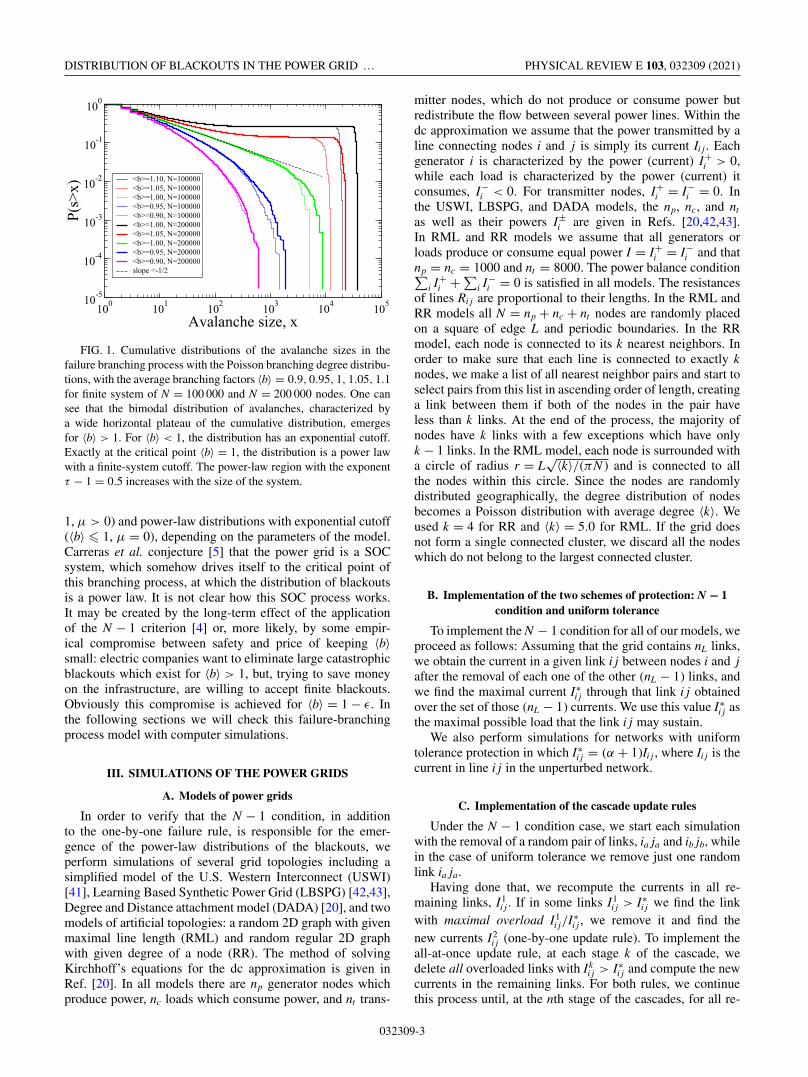
In the second class of initial attacks, such as in the abovementioned discussion of power grids [6–8,13,18] and a recentwork on the Motter and Lai model [26], the cascade is startedby the failure of a single element. Here it is informative tostudy the distribution of the “blackout” sizes, i.e., the num-ber of nodes that failed during the cascade and how sucha probability distribution depends on the model parameters.In this case the system before the attack exists in a statecharacterized by some set of parameters, but the parameterp describing the size of the initial attack is not applicable atall. In this case, in both topological and overload models, thecascading failures evolve as a branching process in which thefailure of one element leads to the failure of b elements, whichdepend on the failed element in the topological models, orget overloaded due to the removal of the failed element in theoverload models. The critical point of the simplest branchingprocess with a fixed distribution of the branching factor P(b) isdefined by 〈b〉 = 1 [39]. For the mean-field variant of the fixeddistribution model, the distribution of the avalanche sizes is apower law with an exponential cutoff P(s) ∼ s−τ exp(−s/s∗),where s∗ ∼ (〈b〉 − 1)−1/σ . Here σ = 1/2 and τ = 3/2 arethe critical exponents [17,40]. These in turn give the valuesof the two other critical exponents, γ = (2 − τ )/σ = 1 andβ = (τ − 1)/σ = 1, where γ governs the divergence of theaverage finite avalanche size for 〈b〉 → 1 and β governs theprobability of a giant avalanche for 〈b〉 > 1, i.e., the avalanchewhich in the thermodynamic limit N → ∞ constitutes a finitefraction μ of the entire system. Note that μ plays the roleof the order parameter of the phase transition. This phasetransition is the second-order transition as in percolation. For〈b〉 > 1, μ > 0, while for 〈b〉 � 1, μ = 0. In a finite network,the size of the giant avalanche fluctuates around μN and,thus, forms the second peak of the bimodal distribution ofavalanche sizes. Other avalanches, which do not scale as afinite fraction of the network, form a first peak of the sizedistributions, which is separated from the second peak by ahuge gap because there are no avalanches of size s, such thats∗ << s << μN (Fig. 1). Thus, this simple branching processmodel predicts the existence of regimes with bimodal (〈b〉 >

032309-2

DISTRIBUTION OF BLACKOUTS IN THE POWER GRID … PHYSICAL REVIEW E 103, 032309 (2021)

100

101

102

103

104

105

Avalanche size, x

10-5

10-4

10-3

10-2

10-1

100

P(s

>x)

<b>=1.10, N=100000<b>=1.05, N=100000<b>=1.00, N=100000<b>=0.95, N=100000<b>=0.90, N=100000<b>=1.00, N=200000<b>=1.05, N=200000<b>=1.00, N=200000<b>=0.95, N=200000<b>=0.90, N=200000slope =-1/2

FIG. 1. Cumulative distributions of the avalanche sizes in thefailure branching process with the Poisson branching degree distribu-tions, with the average branching factors 〈b〉 = 0.9, 0.95, 1, 1.05, 1.1for finite system of N = 100 000 and N = 200 000 nodes. One cansee that the bimodal distribution of avalanches, characterized bya wide horizontal plateau of the cumulative distribution, emergesfor 〈b〉 > 1. For 〈b〉 < 1, the distribution has an exponential cutoff.Exactly at the critical point 〈b〉 = 1, the distribution is a power lawwith a finite-system cutoff. The power-law region with the exponentτ − 1 = 0.5 increases with the size of the system.

1, μ > 0) and power-law distributions with exponential cutoff(〈b〉 � 1, μ = 0), depending on the parameters of the model.Carreras et al. conjecture [5] that the power grid is a SOCsystem, which somehow drives itself to the critical point ofthis branching process, at which the distribution of blackoutsis a power law. It is not clear how this SOC process works.It may be created by the long-term effect of the applicationof the N − 1 criterion [4] or, more likely, by some empir-ical compromise between safety and price of keeping 〈b〉small: electric companies want to eliminate large catastrophicblackouts which exist for 〈b〉 > 1, but, trying to save moneyon the infrastructure, are willing to accept finite blackouts.Obviously this compromise is achieved for 〈b〉 = 1 − ε. Inthe following sections we will check this failure-branchingprocess model with computer simulations.

III. SIMULATIONS OF THE POWER GRIDS

A. Models of power grids

In order to verify that the N − 1 condition, in additionto the one-by-one failure rule, is responsible for the emer-gence of the power-law distributions of the blackouts, weperform simulations of several grid topologies including asimplified model of the U.S. Western Interconnect (USWI)[41], Learning Based Synthetic Power Grid (LBSPG) [42,43],Degree and Distance attachment model (DADA) [20], and twomodels of artificial topologies: a random 2D graph with givenmaximal line length (RML) and random regular 2D graphwith given degree of a node (RR). The method of solvingKirchhoff’s equations for the dc approximation is given inRef. [20]. In all models there are np generator nodes whichproduce power, nc loads which consume power, and nt trans-

mitter nodes, which do not produce or consume power butredistribute the flow between several power lines. Within thedc approximation we assume that the power transmitted by aline connecting nodes i and j is simply its current Ii j . Eachgenerator i is characterized by the power (current) I+

i > 0,while each load is characterized by the power (current) itconsumes, I−

i < 0. For transmitter nodes, I+i = I−

i = 0. Inthe USWI, LBSPG, and DADA models, the np, nc, and nt

as well as their powers I±i are given in Refs. [20,42,43].

In RML and RR models we assume that all generators orloads produce or consume equal power I = I+

i = I−i and that

np = nc = 1000 and nt = 8000. The power balance condition∑i I+

i + ∑i I−

i = 0 is satisfied in all models. The resistancesof lines Ri j are proportional to their lengths. In the RML andRR models all N = np + nc + nt nodes are randomly placedon a square of edge L and periodic boundaries. In the RRmodel, each node is connected to its k nearest neighbors. Inorder to make sure that each line is connected to exactly knodes, we make a list of all nearest neighbor pairs and start toselect pairs from this list in ascending order of length, creatinga link between them if both of the nodes in the pair haveless than k links. At the end of the process, the majority ofnodes have k links with a few exceptions which have onlyk − 1 links. In the RML model, each node is surrounded witha circle of radius r = L

√〈k〉/(πN ) and is connected to allthe nodes within this circle. Since the nodes are randomlydistributed geographically, the degree distribution of nodesbecomes a Poisson distribution with average degree 〈k〉. Weused k = 4 for RR and 〈k〉 = 5.0 for RML. If the grid doesnot form a single connected cluster, we discard all the nodeswhich do not belong to the largest connected cluster.

B. Implementation of the two schemes of protection: N − 1condition and uniform tolerance

To implement the N − 1 condition for all of our models, weproceed as follows: Assuming that the grid contains nL links,we obtain the current in a given link i j between nodes i and jafter the removal of each one of the other (nL − 1) links, andwe find the maximal current I∗

i j through that link i j obtainedover the set of those (nL − 1) currents. We use this value I∗

i j asthe maximal possible load that the link i j may sustain.

We also perform simulations for networks with uniformtolerance protection in which I∗

i j = (α + 1)Ii j , where Ii j is thecurrent in line i j in the unperturbed network.

C. Implementation of the cascade update rules

Under the N − 1 condition case, we start each simulationwith the removal of a random pair of links, ia ja and ib jb, whilein the case of uniform tolerance we remove just one randomlink ia ja.

Having done that, we recompute the currents in all re-maining links, I1

i j . If in some links I1i j > I∗

i j we find the linkwith maximal overload I1

i j/I∗i j , we remove it and find the

new currents I2i j (one-by-one update rule). To implement the

all-at-once update rule, at each stage k of the cascade, wedelete all overloaded links with Ik

i j > I∗i j and compute the new

currents in the remaining links. For both rules, we continuethis process until, at the nth stage of the cascades, for all re-

032309-3

YOSEF KORNBLUTH et al. PHYSICAL REVIEW E 103, 032309 (2021)

maining links, Ini j � I∗

i j . If, at a certain stage, the grid splits intoseveral disconnected clusters, we apply the power production-consumption equalization for each cluster using the minimalproduction-consumption rule described in Ref. [20]. We com-pute the blackout size as a fraction of the consumed powerlost in the cascade |I0 − I f |/I0, where I0 = ∑

i |I−i | for the

intact grid and I f = ∑i |I−

i | at the end of the cascade. Anothermethod of measuring the blackout size is to compute thefraction of the lines lost in the cascade fd = nd/nL, where nd

is the number of lines removed from the grid due to overload.In summary, for each network model, we study four cases:

the N − 1 condition together with one-by-one or all-at-onceupdate rules, and uniform tolerance together with one-by-oneor all-at-once update rules.

D. Results for different models of power gridwith the N − 1 condition

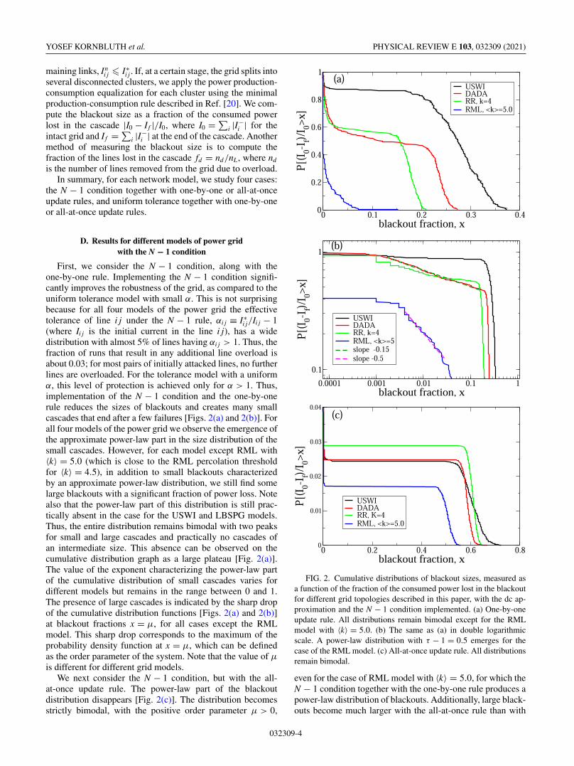
First, we consider the N − 1 condition, along with theone-by-one rule. Implementing the N − 1 condition signifi-cantly improves the robustness of the grid, as compared to theuniform tolerance model with small α. This is not surprisingbecause for all four models of the power grid the effectivetolerance of line i j under the N − 1 rule, αi j ≡ I∗

i j/Ii j − 1(where Ii j is the initial current in the line i j), has a widedistribution with almost 5% of lines having αi j > 1. Thus, thefraction of runs that result in any additional line overload isabout 0.03; for most pairs of initially attacked lines, no furtherlines are overloaded. For the tolerance model with a uniformα, this level of protection is achieved only for α > 1. Thus,implementation of the N − 1 condition and the one-by-onerule reduces the sizes of blackouts and creates many smallcascades that end after a few failures [Figs. 2(a) and 2(b)]. Forall four models of the power grid we observe the emergence ofthe approximate power-law part in the size distribution of thesmall cascades. However, for each model except RML with〈k〉 = 5.0 (which is close to the RML percolation thresholdfor 〈k〉 = 4.5), in addition to small blackouts characterizedby an approximate power-law distribution, we still find somelarge blackouts with a significant fraction of power loss. Notealso that the power-law part of this distribution is still prac-tically absent in the case for the USWI and LBSPG models.Thus, the entire distribution remains bimodal with two peaksfor small and large cascades and practically no cascades ofan intermediate size. This absence can be observed on thecumulative distribution graph as a large plateau [Fig. 2(a)].The value of the exponent characterizing the power-law partof the cumulative distribution of small cascades varies fordifferent models but remains in the range between 0 and 1.The presence of large cascades is indicated by the sharp dropof the cumulative distribution functions [Figs. 2(a) and 2(b)]at blackout fractions x = μ, for all cases except the RMLmodel. This sharp drop corresponds to the maximum of theprobability density function at x = μ, which can be definedas the order parameter of the system. Note that the value of μ

is different for different grid models.We next consider the N − 1 condition, but with the all-

at-once update rule. The power-law part of the blackoutdistribution disappears [Fig. 2(c)]. The distribution becomesstrictly bimodal, with the positive order parameter μ > 0,

FIG. 2. Cumulative distributions of blackout sizes, measured asa function of the fraction of the consumed power lost in the blackoutfor different grid topologies described in this paper, with the dc ap-proximation and the N − 1 condition implemented. (a) One-by-oneupdate rule. All distributions remain bimodal except for the RMLmodel with 〈k〉 = 5.0. (b) The same as (a) in double logarithmicscale. A power-law distribution with τ − 1 = 0.5 emerges for thecase of the RML model. (c) All-at-once update rule. All distributionsremain bimodal.

even for the case of RML model with 〈k〉 = 5.0, for which theN − 1 condition together with the one-by-one rule produces apower-law distribution of blackouts. Additionally, large black-outs become much larger with the all-at-once rule than with

032309-4

DISTRIBUTION OF BLACKOUTS IN THE POWER GRID … PHYSICAL REVIEW E 103, 032309 (2021)

the one-by-one rule; the system is more prone to failure, whichis indicated by the larger values of the order parameter μ.

E. Comparison of different cascade models for the USWIand the LBSPG

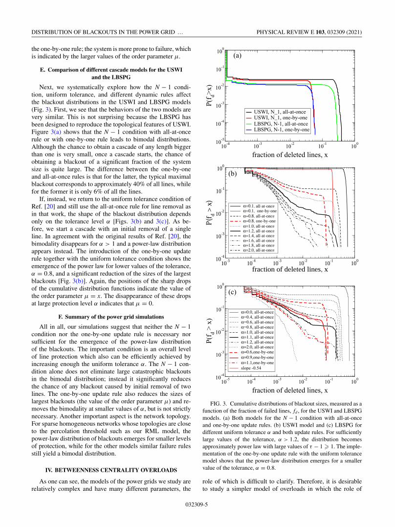
Next, we systematically explore how the N − 1 condi-tion, uniform tolerance, and different dynamic rules affectthe blackout distributions in the USWI and LBSPG models(Fig. 3). First, we see that the behaviors of the two models arevery similar. This is not surprising because the LBSPG hasbeen designed to reproduce the topological features of USWI.Figure 3(a) shows that the N − 1 condition with all-at-oncerule or with one-by-one rule leads to bimodal distributions.Although the chance to obtain a cascade of any length biggerthan one is very small, once a cascade starts, the chance ofobtaining a blackout of a significant fraction of the systemsize is quite large. The difference between the one-by-oneand all-at-once rules is that for the latter, the typical maximalblackout corresponds to approximately 40% of all lines, whilefor the former it is only 6% of all the lines.

If, instead, we return to the uniform tolerance condition ofRef. [20] and still use the all-at-once rule for line removal asin that work, the shape of the blackout distribution dependsonly on the tolerance level α [Figs. 3(b) and 3(c)]. As be-fore, we start a cascade with an initial removal of a singleline. In agreement with the original results of Ref. [20], thebimodality disappears for α > 1 and a power-law distributionappears instead. The introduction of the one-by-one updaterule together with the uniform tolerance condition shows theemergence of the power law for lower values of the tolerance,α = 0.8, and a significant reduction of the sizes of the largestblackouts [Fig. 3(b)]. Again, the positions of the sharp dropsof the cumulative distribution functions indicate the value ofthe order parameter μ = x. The disappearance of these dropsat large protection level α indicates that μ = 0.

F. Summary of the power grid simulations

All in all, our simulations suggest that neither the N − 1condition nor the one-by-one update rule is necessary norsufficient for the emergence of the power-law distributionof the blackouts. The important condition is an overall levelof line protection which also can be efficiently achieved byincreasing enough the uniform tolerance α. The N − 1 con-dition alone does not eliminate large catastrophic blackoutsin the bimodal distribution; instead it significantly reducesthe chance of any blackout caused by initial removal of twolines. The one-by-one update rule also reduces the sizes oflargest blackouts (the value of the order parameter μ) and re-moves the bimodality at smaller values of α, but is not strictlynecessary. Another important aspect is the network topology.For sparse homogeneous networks whose topologies are closeto the percolation threshold such as our RML model, thepower-law distribution of blackouts emerges for smaller levelsof protection, while for the other models similar failure rulesstill yield a bimodal distribution.

IV. BETWEENNESS CENTRALITY OVERLOADS

As one can see, the models of the power grids we study arerelatively complex and have many different parameters, the

FIG. 3. Cumulative distributions of blackout sizes, measured as afunction of the fraction of failed lines, fd , for the USWI and LBSPGmodels. (a) Both models for the N − 1 condition with all-at-onceand one-by-one update rules. (b) USWI model and (c) LBSPG fordifferent uniform tolerance α and both update rules. For sufficientlylarge values of the tolerance, α > 1.2, the distribution becomesapproximately power law with large values of τ − 1 � 1. The imple-mentation of the one-by-one update rule with the uniform tolerancemodel shows that the power-law distribution emerges for a smallervalue of the tolerance, α = 0.8.

role of which is difficult to clarify. Therefore, it is desirableto study a simpler model of overloads in which the role of

032309-5

YOSEF KORNBLUTH et al. PHYSICAL REVIEW E 103, 032309 (2021)

each parameter becomes clear. It is also interesting to see ifthe emergence of the power-law distribution is a universalphenomenon for different overload models. A good candi-date for such a model is the betweenness centrality model,which displays a clear bimodal distribution of blackouts forthe all-at-once removal rule and uniform tolerance conditionemployed by Motter and Lai [22,26]. However, we can expectthat, similarly to the power grid models, the implementationof the N − 1 condition and one-by-one removal rule in thebetweenness centrality model will also lead to the emergenceof a power-law distribution of the blackout sizes. Testing ofthis hypothesis will allow us to better understand the generalmechanism of the emergence of the power-law distribution ofthe sizes of blackouts in the overload models.

A. Implementation of the betweenness centrality model

We build the betweenness centrality model as in Ref. [37].Namely, we create a randomly connected graph with a givendegree distribution P(k) and compute the shortest paths be-tween each pair of nodes. The length of each edge is assumedto be equal to 1 + ε, where ε is a normally distributed randomvariable with a small standard deviation σε 1. This precau-tion is taken in order to make sure that each pair of nodes i jhas a unique shortest path connecting them. The betweennesscentrality b(k) of each node k is computed as the number ofall shortest paths i j passing through node k, such that k �= i,k �= j.

B. Implementation of the N − 1 condition

The N − 1 condition in the betweenness centrality modelshould be understood in the following way: If any one nodei is deleted, the rest of the nodes remain connected and thebetweenness centrality of each remaining node j, bi( j) doesnot exceed its maximal possible load b∗( j). Thus

b∗( j) = maxi �= j

bi( j), (1)

and the original graph must be biconnected. Note that inthe original Motter and Lai model with a uniform toleranceα > 0,

b∗( j) = (1 + α)b( j), (2)

where b( j) is the initial betweenness of node j in a completelyintact network.

To implement this model, we first construct a randomlyconnected graph of N nodes with a given degree distribu-tion P(k) with the Molloy-Read algorithm [44] and findits largest biconnected component with Nb nodes using theHopcroft-Tarjan algorithm [45]. After that, we compute thebetweenness centrality of each node and repeat Nb simulationswith each node removed in turn to find b∗(i) for each node.To find the distribution of cascades of failures we remove apair of random nodes and find the nodes i with overloadsz = b(i)/b∗(i) > 1. In the first case of all-at-once removal,at each stage of the cascade we remove all the nodes withoverloads, recompute the betweenness centrality of the re-maining nodes and repeat this process until no overloadednodes are left. In the second case of one-by-one removal,at each stage of the cascades we remove only one of the

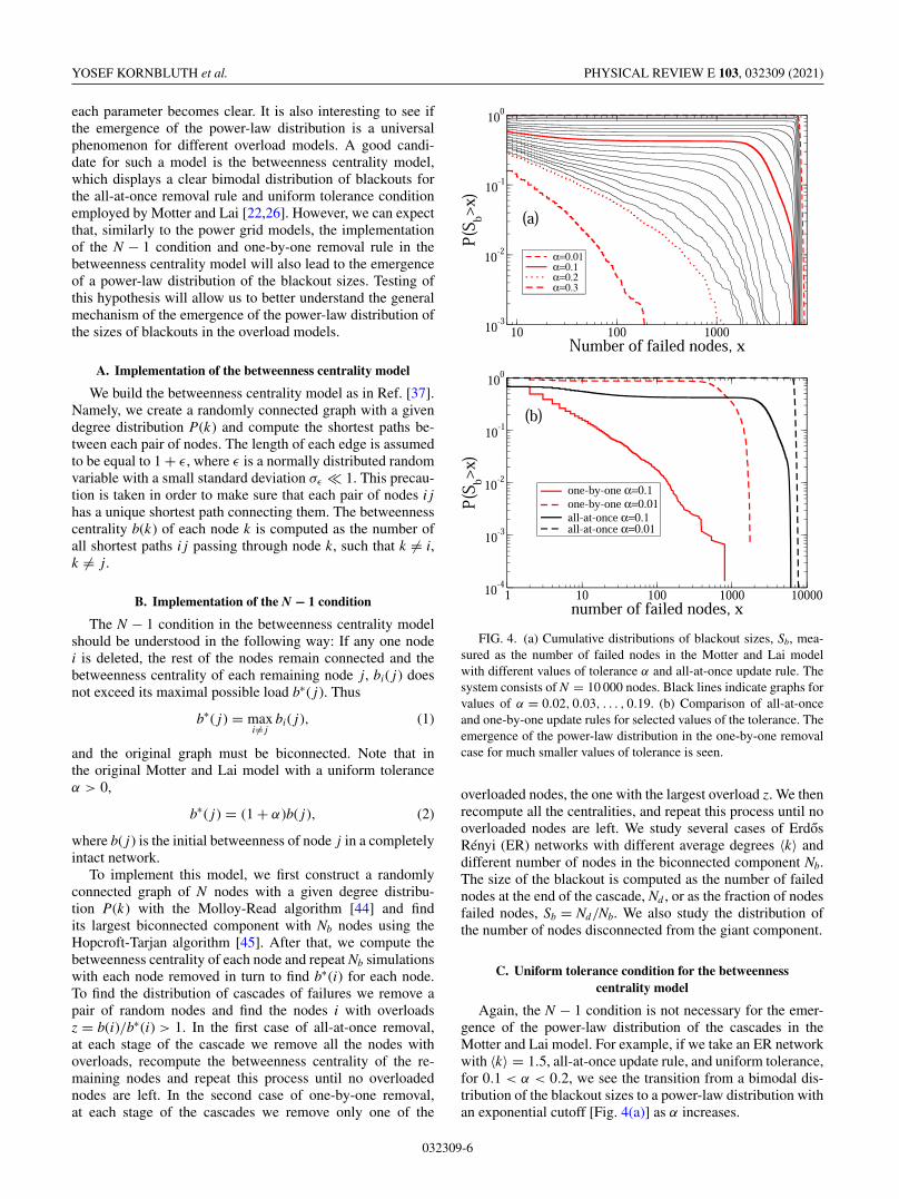
FIG. 4. (a) Cumulative distributions of blackout sizes, Sb, mea-sured as the number of failed nodes in the Motter and Lai modelwith different values of tolerance α and all-at-once update rule. Thesystem consists of N = 10 000 nodes. Black lines indicate graphs forvalues of α = 0.02, 0.03, . . . , 0.19. (b) Comparison of all-at-onceand one-by-one update rules for selected values of the tolerance. Theemergence of the power-law distribution in the one-by-one removalcase for much smaller values of tolerance is seen.

overloaded nodes, the one with the largest overload z. We thenrecompute all the centralities, and repeat this process until nooverloaded nodes are left. We study several cases of ErdosRényi (ER) networks with different average degrees 〈k〉 anddifferent number of nodes in the biconnected component Nb.The size of the blackout is computed as the number of failednodes at the end of the cascade, Nd , or as the fraction of nodesfailed nodes, Sb = Nd/Nb. We also study the distribution ofthe number of nodes disconnected from the giant component.

C. Uniform tolerance condition for the betweennesscentrality model

Again, the N − 1 condition is not necessary for the emer-gence of the power-law distribution of the cascades in theMotter and Lai model. For example, if we take an ER networkwith 〈k〉 = 1.5, all-at-once update rule, and uniform tolerance,for 0.1 < α < 0.2, we see the transition from a bimodal dis-tribution of the blackout sizes to a power-law distribution withan exponential cutoff [Fig. 4(a)] as α increases.

032309-6

DISTRIBUTION OF BLACKOUTS IN THE POWER GRID … PHYSICAL REVIEW E 103, 032309 (2021)

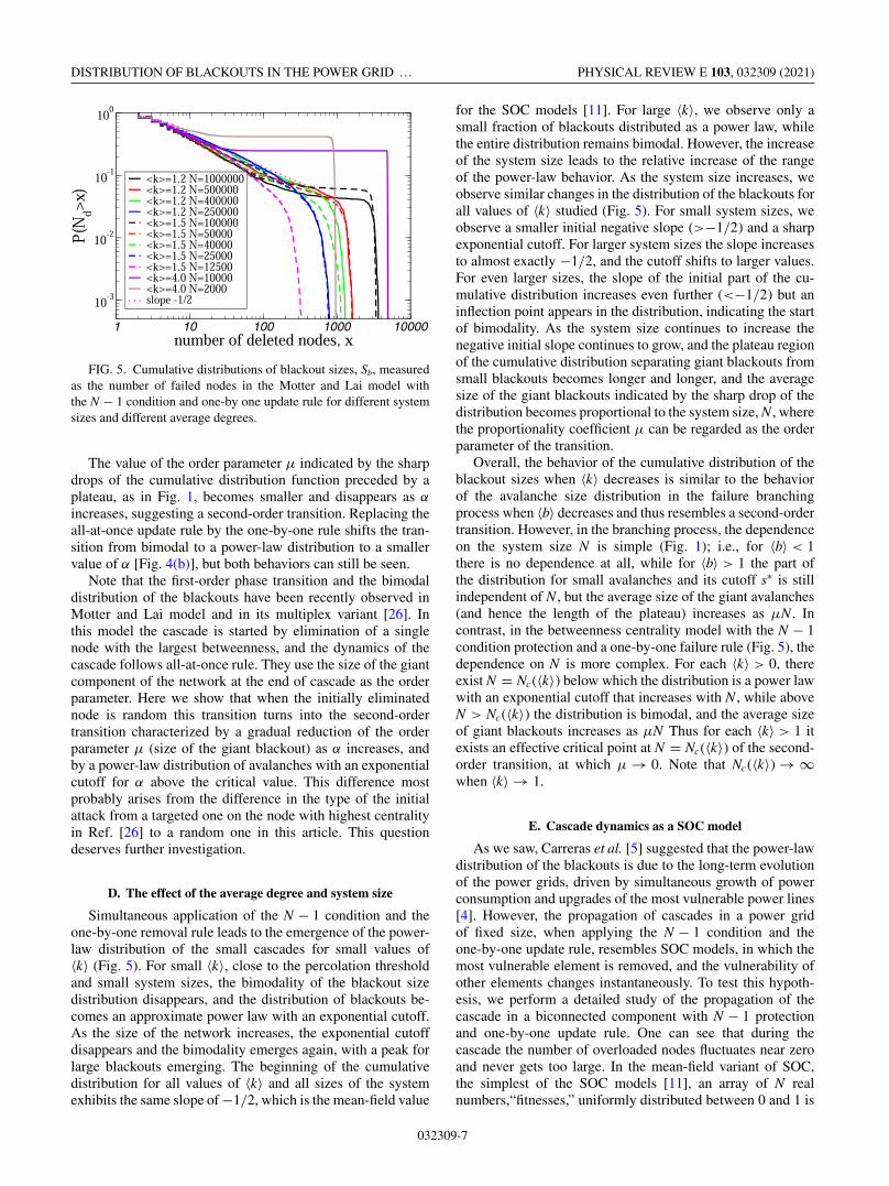
FIG. 5. Cumulative distributions of blackout sizes, Sb, measuredas the number of failed nodes in the Motter and Lai model withthe N − 1 condition and one-by one update rule for different systemsizes and different average degrees.

The value of the order parameter μ indicated by the sharpdrops of the cumulative distribution function preceded by aplateau, as in Fig. 1, becomes smaller and disappears as α

increases, suggesting a second-order transition. Replacing theall-at-once update rule by the one-by-one rule shifts the tran-sition from bimodal to a power-law distribution to a smallervalue of α [Fig. 4(b)], but both behaviors can still be seen.

Note that the first-order phase transition and the bimodaldistribution of the blackouts have been recently observed inMotter and Lai model and in its multiplex variant [26]. Inthis model the cascade is started by elimination of a singlenode with the largest betweenness, and the dynamics of thecascade follows all-at-once rule. They use the size of the giantcomponent of the network at the end of cascade as the orderparameter. Here we show that when the initially eliminatednode is random this transition turns into the second-ordertransition characterized by a gradual reduction of the orderparameter μ (size of the giant blackout) as α increases, andby a power-law distribution of avalanches with an exponentialcutoff for α above the critical value. This difference mostprobably arises from the difference in the type of the initialattack from a targeted one on the node with highest centralityin Ref. [26] to a random one in this article. This questiondeserves further investigation.

D. The effect of the average degree and system size

Simultaneous application of the N − 1 condition and theone-by-one removal rule leads to the emergence of the power-law distribution of the small cascades for small values of〈k〉 (Fig. 5). For small 〈k〉, close to the percolation thresholdand small system sizes, the bimodality of the blackout sizedistribution disappears, and the distribution of blackouts be-comes an approximate power law with an exponential cutoff.As the size of the network increases, the exponential cutoffdisappears and the bimodality emerges again, with a peak forlarge blackouts emerging. The beginning of the cumulativedistribution for all values of 〈k〉 and all sizes of the systemexhibits the same slope of −1/2, which is the mean-field value

for the SOC models [11]. For large 〈k〉, we observe only asmall fraction of blackouts distributed as a power law, whilethe entire distribution remains bimodal. However, the increaseof the system size leads to the relative increase of the rangeof the power-law behavior. As the system size increases, weobserve similar changes in the distribution of the blackouts forall values of 〈k〉 studied (Fig. 5). For small system sizes, weobserve a smaller initial negative slope (>−1/2) and a sharpexponential cutoff. For larger system sizes the slope increasesto almost exactly −1/2, and the cutoff shifts to larger values.For even larger sizes, the slope of the initial part of the cu-mulative distribution increases even further (<−1/2) but aninflection point appears in the distribution, indicating the startof bimodality. As the system size continues to increase thenegative initial slope continues to grow, and the plateau regionof the cumulative distribution separating giant blackouts fromsmall blackouts becomes longer and longer, and the averagesize of the giant blackouts indicated by the sharp drop of thedistribution becomes proportional to the system size, N , wherethe proportionality coefficient μ can be regarded as the orderparameter of the transition.

Overall, the behavior of the cumulative distribution of theblackout sizes when 〈k〉 decreases is similar to the behaviorof the avalanche size distribution in the failure branchingprocess when 〈b〉 decreases and thus resembles a second-ordertransition. However, in the branching process, the dependenceon the system size N is simple (Fig. 1); i.e., for 〈b〉 < 1there is no dependence at all, while for 〈b〉 > 1 the part ofthe distribution for small avalanches and its cutoff s∗ is stillindependent of N , but the average size of the giant avalanches(and hence the length of the plateau) increases as μN . Incontrast, in the betweenness centrality model with the N − 1condition protection and a one-by-one failure rule (Fig. 5), thedependence on N is more complex. For each 〈k〉 > 0, thereexist N = Nc(〈k〉) below which the distribution is a power lawwith an exponential cutoff that increases with N , while aboveN > Nc(〈k〉) the distribution is bimodal, and the average sizeof giant blackouts increases as μN Thus for each 〈k〉 > 1 itexists an effective critical point at N = Nc(〈k〉) of the second-order transition, at which μ → 0. Note that Nc(〈k〉) → ∞when 〈k〉 → 1.

E. Cascade dynamics as a SOC model

As we saw, Carreras et al. [5] suggested that the power-lawdistribution of the blackouts is due to the long-term evolutionof the power grids, driven by simultaneous growth of powerconsumption and upgrades of the most vulnerable power lines[4]. However, the propagation of cascades in a power gridof fixed size, when applying the N − 1 condition and theone-by-one update rule, resembles SOC models, in which themost vulnerable element is removed, and the vulnerability ofother elements changes instantaneously. To test this hypoth-esis, we perform a detailed study of the propagation of thecascade in a biconnected component with N − 1 protectionand one-by-one update rule. One can see that during thecascade the number of overloaded nodes fluctuates near zeroand never gets too large. In the mean-field variant of SOC,the simplest of the SOC models [11], an array of N realnumbers,“fitnesses,” uniformly distributed between 0 and 1 is

032309-7

YOSEF KORNBLUTH et al. PHYSICAL REVIEW E 103, 032309 (2021)

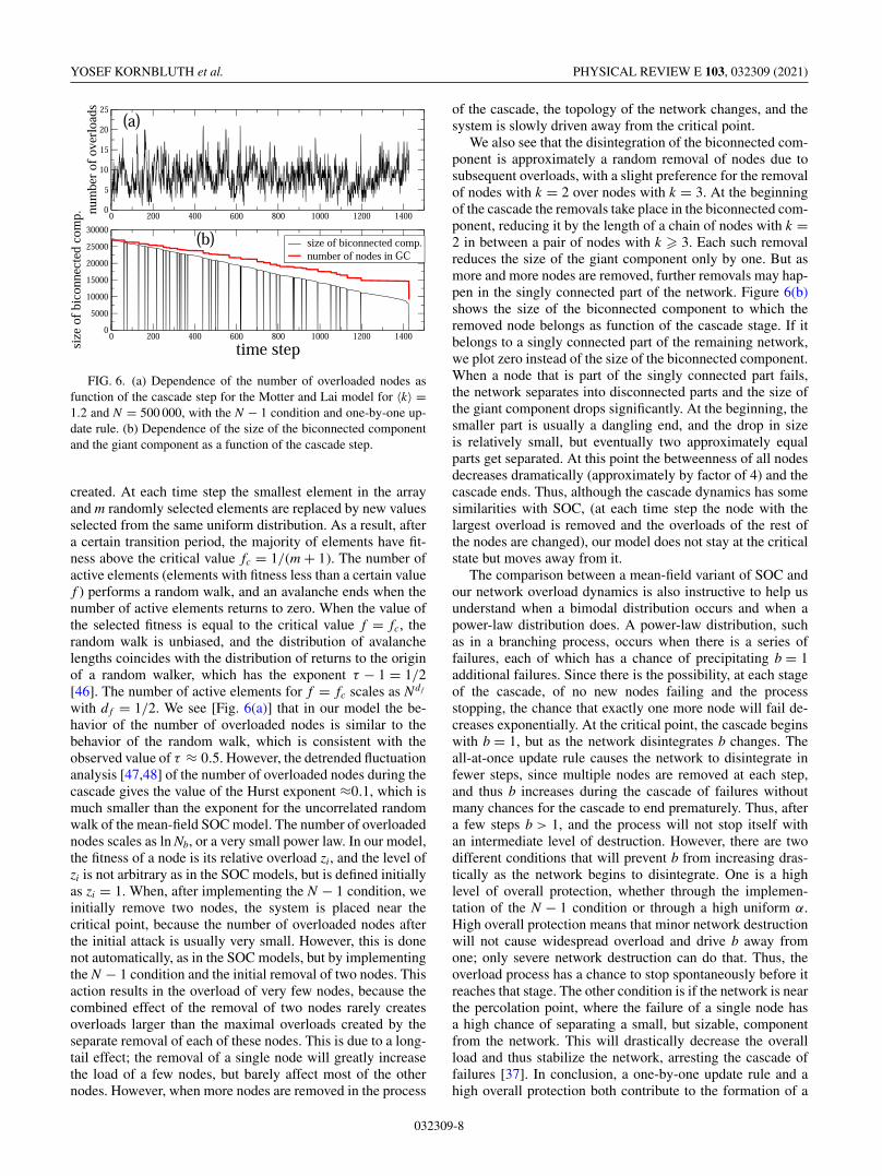
FIG. 6. (a) Dependence of the number of overloaded nodes asfunction of the cascade step for the Motter and Lai model for 〈k〉 =1.2 and N = 500 000, with the N − 1 condition and one-by-one up-date rule. (b) Dependence of the size of the biconnected componentand the giant component as a function of the cascade step.

created. At each time step the smallest element in the arrayand m randomly selected elements are replaced by new valuesselected from the same uniform distribution. As a result, aftera certain transition period, the majority of elements have fit-ness above the critical value fc = 1/(m + 1). The number ofactive elements (elements with fitness less than a certain valuef ) performs a random walk, and an avalanche ends when thenumber of active elements returns to zero. When the value ofthe selected fitness is equal to the critical value f = fc, therandom walk is unbiased, and the distribution of avalanchelengths coincides with the distribution of returns to the originof a random walker, which has the exponent τ − 1 = 1/2[46]. The number of active elements for f = fc scales as Nd f

with d f = 1/2. We see [Fig. 6(a)] that in our model the be-havior of the number of overloaded nodes is similar to thebehavior of the random walk, which is consistent with theobserved value of τ ≈ 0.5. However, the detrended fluctuationanalysis [47,48] of the number of overloaded nodes during thecascade gives the value of the Hurst exponent ≈0.1, which ismuch smaller than the exponent for the uncorrelated randomwalk of the mean-field SOC model. The number of overloadednodes scales as ln Nb, or a very small power law. In our model,the fitness of a node is its relative overload zi, and the level ofzi is not arbitrary as in the SOC models, but is defined initiallyas zi = 1. When, after implementing the N − 1 condition, weinitially remove two nodes, the system is placed near thecritical point, because the number of overloaded nodes afterthe initial attack is usually very small. However, this is donenot automatically, as in the SOC models, but by implementingthe N − 1 condition and the initial removal of two nodes. Thisaction results in the overload of very few nodes, because thecombined effect of the removal of two nodes rarely createsoverloads larger than the maximal overloads created by theseparate removal of each of these nodes. This is due to a long-tail effect; the removal of a single node will greatly increasethe load of a few nodes, but barely affect most of the othernodes. However, when more nodes are removed in the process

of the cascade, the topology of the network changes, and thesystem is slowly driven away from the critical point.

We also see that the disintegration of the biconnected com-ponent is approximately a random removal of nodes due tosubsequent overloads, with a slight preference for the removalof nodes with k = 2 over nodes with k = 3. At the beginningof the cascade the removals take place in the biconnected com-ponent, reducing it by the length of a chain of nodes with k =2 in between a pair of nodes with k � 3. Each such removalreduces the size of the giant component only by one. But asmore and more nodes are removed, further removals may hap-pen in the singly connected part of the network. Figure 6(b)shows the size of the biconnected component to which theremoved node belongs as function of the cascade stage. If itbelongs to a singly connected part of the remaining network,we plot zero instead of the size of the biconnected component.When a node that is part of the singly connected part fails,the network separates into disconnected parts and the size ofthe giant component drops significantly. At the beginning, thesmaller part is usually a dangling end, and the drop in sizeis relatively small, but eventually two approximately equalparts get separated. At this point the betweenness of all nodesdecreases dramatically (approximately by factor of 4) and thecascade ends. Thus, although the cascade dynamics has somesimilarities with SOC, (at each time step the node with thelargest overload is removed and the overloads of the rest ofthe nodes are changed), our model does not stay at the criticalstate but moves away from it.

The comparison between a mean-field variant of SOC andour network overload dynamics is also instructive to help usunderstand when a bimodal distribution occurs and when apower-law distribution does. A power-law distribution, suchas in a branching process, occurs when there is a series offailures, each of which has a chance of precipitating b = 1additional failures. Since there is the possibility, at each stageof the cascade, of no new nodes failing and the processstopping, the chance that exactly one more node will fail de-creases exponentially. At the critical point, the cascade beginswith b = 1, but as the network disintegrates b changes. Theall-at-once update rule causes the network to disintegrate infewer steps, since multiple nodes are removed at each step,and thus b increases during the cascade of failures withoutmany chances for the cascade to end prematurely. Thus, aftera few steps b > 1, and the process will not stop itself withan intermediate level of destruction. However, there are twodifferent conditions that will prevent b from increasing dras-tically as the network begins to disintegrate. One is a highlevel of overall protection, whether through the implemen-tation of the N − 1 condition or through a high uniform α.High overall protection means that minor network destructionwill not cause widespread overload and drive b away fromone; only severe network destruction can do that. Thus, theoverload process has a chance to stop spontaneously before itreaches that stage. The other condition is if the network is nearthe percolation point, where the failure of a single node hasa high chance of separating a small, but sizable, componentfrom the network. This will drastically decrease the overallload and thus stabilize the network, arresting the cascade offailures [37]. In conclusion, a one-by-one update rule and ahigh overall protection both contribute to the formation of a

032309-8

DISTRIBUTION OF BLACKOUTS IN THE POWER GRID … PHYSICAL REVIEW E 103, 032309 (2021)

power law. The effect of the system size discussed above canalso be understood in light of the comparison to a branchingprocess. The larger the system, the more nodes (as an absolutenumber, not a fraction) fail following the initial attack. Thus,the chance that none of the overloaded nodes will cause an-other node to overload (i.e., a spontaneous end to the cascade)becomes increasingly unlikely as the number of overloadednodes increases, even if b remains close to one for many stepsof the cascade. Thus, the chance that the cascade of failureswill end with an intermediate amount of damage becomesmore unlikely when the size of the original system increases.

V. DISCUSSION AND CONCLUSION

We have shown that the dc model of the power grid hasremarkable similarities to the Motter and Lai model of be-tweenness centrality, suggesting that the exact physical lawsgoverning the flux do not play as big a role as the networktopology and the dynamics of the cascade propagation. Wehave shown that both overload models have similarities anddifferences with the topological models [27–34]. In the topo-logical models the outcome of the cascade depends only onthe topology of the network and the location of the initialdamage, while in the overload models the outcome signifi-cantly depends on the dynamics of the cascade, which itselfdepends on the order of removal of overloaded elements andthe relative speed of failure of overloaded elements and re-distribution of flux after the failure. In general, if the failureis slow compared to the redistribution of flux (one-by-oneremoval rule) the cascades become smaller, while for fastfailures of overloaded elements (the all-at-once removal rule)the blackouts can be larger by an order of magnitude thanin the one-by-one case. But the one-by-one removal rule isneither necessary nor sufficient for the elimination of “giant”blackouts engulfing a finite fraction of the entire system.

We also find that the N − 1 condition is neither neces-sary nor sufficient for the disappearance of large cascadesdestroying a finite fraction of the elements in the system, but itreduces the probability of any cascade by an order of magni-tude compared to the universal tolerance condition even for alarge tolerance α, if two elements are deleted simultaneouslyat the beginning of the cascade.

The general picture of the behavior of the overload modelsis consistent with the simple model of the failure branchingprocess, which demonstrates a second-order phase transition.For large protection levels (small 〈b〉) the distribution ofblackout sizes is a power law with exponential cutoff, whilefor low protection levels (large 〈b〉) the distribution of black-out sizes becomes bimodal, when a fraction of large blackoutsengulfing a finite fraction of the entire system emerges. Thisfraction and the size of these “giant” blackouts (which serve asthe order parameter of the problem μ) continuously decreasewhen the protection level increases and vanishes when 〈b〉reaches its critical value 〈b〉 = 1.

The protection level can be increased by several factors: (1)increase of the tolerance α, (2) introduction of the one-by-oneremoval rule, (3) the reduction of the network connectivity,i.e., bringing the network closer to the percolation threshold,by reducing the average degree 〈k〉, and (4) by decreasing thesystem size. These methods have an additive effect, i.e., when

applied simultaneously they will achieve larger protectionlevels than when applied separately. For example, applicationof the one-by-one removal rule alone may not change thebimodal distribution of blackouts to unimodal; however, whenimplemented together with the uniform tolerance condition,it will help to achieve the unimodal distribution for smallervalues of the tolerance α.

The empirical observation of the power-law distributionof the blackout sizes in real power grids indicates that thesegrids are near the critical point of the correspondent failurebranching process. However, this is unlikely to be caused bya SOC mechanism in which the model is driven to the criticalpoint by a certain dynamic rule. One hypothesis would be thatit is the N − 1 criterion and the one-by-one update rule thatbrings the grid to the SOC state. However, we observe herethat these two conditions are neither necessary nor sufficientfor the existence of a power-law distribution of blackout sizes.Most likely the power grids are brought to the vicinity ofthe critical point by a risk-price compromise, in which theutilities, with the firm goal of avoiding the catastrophic black-outs that engulf a significant fraction of the entire system,increase the level of protection up to the critical point of thebranching process 〈b〉 < 1, but, in order to minimize costsunder this condition, allow 〈b〉 to be as close as possible tothe critical point from below, so that limited but occasionallyvery large blackouts are still possible. It is still desirable todevelop a model of long time evolution of power grids similarto Ref. [4], which reproduces the power-law distribution ofavalanches. The observation of power-law distribution of theblackouts in the sparse networks close to the percolation pointalso emphasizes the role of islanding for preventing largeblackouts.

A plausible reason for the emergence of the power-lawdistribution of cascades is presented in a recent work of Nestiet al. [18], who relate it to the power-law distribution of citysizes and hence the distribution of loads (“sinks”) in the dcapproximation of the grid. They observe τ > 2 in agreementwith empirical observations [5]. However, our study suggeststhat the distribution of loads is irrelevant for the emergence ofthe power-law distribution of blackouts for large protectionlevels. In fact, the USWI model has a lognormal distribu-tion of the loads I−

i with a sharp cutoff, while the LBSPGmodel has a power-law distribution P(|I−

i |) ∼ |I−i |−2.2 of the

loads, but their behavior is very similar in our study, and inboth models the transition from a bimodal distribution to apower-law distribution of the blackouts occurs at high level ofprotection (high tolerance). The appearance of the power-lawdistribution of blackouts also in the Motter and Lai modelsuggests that this feature might be a very general phenomenonnot necessarily related to the power-law distribution of theloads.

ACKNOWLEDGMENTS

This material is based upon work supported in part by theU.S. Department of Energy’s Office of Energy Efficiency andRenewable Energy (EERE) under the Solar Energy Technol-ogy Office, ASSIST Initiative Award No. DE-EE0008769,as well as by Defense Threat Reduction Agency grantsHDTRA1-14-1-0017, HDTRA1-19-1-0016. S.V.B. and G.C.

032309-9

YOSEF KORNBLUTH et al. PHYSICAL REVIEW E 103, 032309 (2021)

acknowledge the partial support of this research through theDr. Bernard W. Gamson Computational Science Center atYeshiva College.

APPENDIX

As mentioned in Sec. II A there is a third class of initialattacks in which the system first undergoes a cascade of fail-ures caused by a massive initial attack with p > pt and theorder parameter stabilizes at S(p). This is analogous to the firstclass of initial attacks. Afterwards, the avalanche is startedby the removal of one additional element. In the well-studiedtopological models, it is known [35,36] that

S(p) − S(pt + 0) ∼ (p − pt )1/2, (A1)

where S(pt + 0) is the limit of S(p) for p → pt abovethe step discontinuity. Because in the topological modelsthe order of removal elements does not play any role, theremoval of one element after the system is stabilized atp is identical to the initial removal of pN + 1 elements,where N is the total number of elements in the system.In either situation, the average avalanche size under this

initial conditions is s = N[S(p + 1/N ) − S(p)] ≈ ∂S(p)/∂ p ∼ (p − pt )−1/2. Hence, the avalanche size diverges abovethe transition point pt , with the divergence characterized bythe critical exponent γ = −1/2.

In network theory this transition is called a hybrid tran-sition, but in fact this behavior is completely equivalent tothe mean-field behavior near the spinodal of the first-orderphase transition [49], such as the behavior of the isother-mal compressibility near the spinodal of the gas-liquid phasetransition. This follows from the fact that the isothermalcompressibility is equivalent to the susceptibility in the Isingmodel, which in turn is equivalent to the average cluster sizeat the percolation transition.

The divergence takes place only for p > pt , while for p <

pt the avalanches remain of finite size or do not exist at all,since S(p) = 0 for p < pt . For p → pt + 0, the distributionof the avalanche sizes develops a power-law behavior withan exponential cutoff S∗: P(s) ∼ s−τ exp(−S/S∗) with themean-field exponent τ = 3/2 [35,36], and S∗ ∼ (p − pt )−1/σ

with σ = −1; they, together with γ = −1/2, satisfy a usualpercolation scaling relation γ = (2 − τ )/σ , but with differentγ and σ than in the percolation theory [17,40].

[1] U.S-Canada Power System Outage Task Force: Final report onthe August 14, 2003 blackout in the United States and Canada:Causes and recommendations (Canada, 2004), https://eta-publications.lbl.gov/sites/default/files/2003-blackout-us-canada.pdf.

[2] Report of the enquiry committee on grid disturbance in theNorthern region on 30th July 2012 and in Northern, Easternand North-Eastern region on 31st July 2012 (2012), https://powermin.nic.in/sites/default/files/uploads/GRID_ENQ_REP_6_8_12.pdf.

[3] Report on the Grid Disturbance on 30th July 2012 and GridDisturbance on 31st July 2012 (2012), http://www.cercind.gov.in/2012/orders/Final_Report_Grid_Disturbance.pdf.

[4] H. Ren, I. Dobson, and B. A. Carreras, IEEE Trans. Power Syst.23, 1217 (2008).

[5] B. A. Carreras, D. E. Newman, and I. Dobson, IEEE Trans.Power Syst. 31, 4406 (2016).

[6] B. A. Carreras, V. E. Lynch, I. Dobson, and D. E. Newman,Chaos 12, 985 (2002).

[7] B. A. Carreras, V. E. Lynch, I. Dobson, and D. E. Newman,Chaos 14, 643 (2004).

[8] I. Dobson and L. Lu, IEEE Trans. CAS 39, 762 (1992).[9] P. Bak and K. Sneppen, Phys. Rev. Lett. 71, 4083 (1993).

[10] M. Paczuski, S. Maslov, and P. Bak, Phys. Rev. E 53, 414(1996).

[11] H. Flyvbjerg, K. Sneppen, and P. Bak, Phys. Rev. Lett. 71, 4087(1993).

[12] R. Albert, I. Albert, and G. L. Nakarado, Phys. Rev. E 69,025103(R) (2004).

[13] Y. Yang, T. Nishikawa, and E. Motter, Science 358, eaan3184(2017).

[14] M. Anghel, K. A. Werley, and A. E. Motter, in Proceedings ofthe 2007 40th Annual Hawaii International Conference on Sys-

tem Sciences HICSS’07, Big Island, HI, USA (IEEE, Piscataway,NJ, 2007), p. 113.

[15] H. Cetinay, S. Soltan, F. A. Kuipers, G. Zussman, andP. Van Mieghem, IEEE Trans. Netw. Sci. Eng. 5, 301(2017).

[16] S. Soltan, A. Loh, and G. Zussman, IEEE Trans. Control Netw.Syst. 5, 1424 (2017).

[17] D. Stauffer and A. Aharony, Introduction to Percolation Theory(Taylor and Francis, Philadelphia, 1994). Note that Stauffer andAharony define the distribution of cluster sizes s by counting thenumber of clusters of different sizes N (s) in a finite network,which is characterized by the critical exponent τ = 5/2. Analternative definition, consistent with the notation in the SOCliterature, is the probability p(s) of a randomly selected site tobelong to a cluster of size s. This probability distribution is char-acterized by a power law with an exponent τ ′ = τ − 1 = 3/2.

[18] T. Nesti, F. Sloothaak, and B. Zwart, Phys. Rev. Lett. 125,058301 (2020).

[19] G. K. Zipf, Soc. Forces 28, 340 (1950).[20] R. Spiewak, S. Soltan, Y. Forman, S. V. Buldyrev, and G.

Zussman, Netw. Sci. 6, 448 (2018).[21] S. Pahwa, C. Scoglio, and A. Scala, Sci. Rep. 4, 3694

(2014).[22] A. E. Motter and Y.-C. Lai, Phys. Rev. E 66, 065102(R)

(2002).[23] A. E. Motter, Phys. Rev. Lett. 93, 098701 (2004).[24] S. Soltan, D. Mazauric, and G. Zussman, Proc. ACM e-Energy

14, 195 (2014).[25] P. Hines, E. Cotilla-Sanchez, and S. Blumsack, Chaos 20,

033122 (2010).[26] O. Artime and M. De Domenico, New J. Phys. 22, 093035

(2020).[27] D. J. Watts, Proc. Natl. Acad. Sci. USA 99, 5766 (2002).

032309-10

DISTRIBUTION OF BLACKOUTS IN THE POWER GRID … PHYSICAL REVIEW E 103, 032309 (2021)

[28] J. P. Gleeson and D. J. Cahalane, Proc. SPIE 6601, 66010W(2007).

[29] G. J. Baxter, S. N. Dorogovtsev, A. V. Goltsev, and J. F. F.Mendes, Phys. Rev. E 82, 011103 (2010).

[30] G. J. Baxter, S. N. Dorogovtsev, A. V. Goltsev, and J. F. F.Mendes, Phys. Rev. E 83, 051134 (2011).

[31] S. V. Buldyrev, R. Parshani, G. Paul, H. E. Stanley, and S.Havlin, Nature (London) 464, 1025 (2010).

[32] R. Parshani, S. V. Buldyrev, and S. Havlin, Proc. Natl. Acad.Sci. USA 108, 1007 (2011).

[33] M. A. Di Muro, S. V. Buldyrev, H. E. Stanley, and L. A.Braunstein, Phys. Rev. E 94, 042304 (2016).

[34] M. A. Di Muro, L. D. Valdez, H. H. Aragao Rego, S. V.Buldyrev, H. E. Stanley, and L. A. Braunstein, Sci. Rep. 7,15059 (2017).

[35] S. N. Dorogovtsev, A. V. Goltsev, and J. F. F. Mendes, PhysicaD 224, 7 (2006).

[36] G. J. Baxter, S. N. Dorogovtsev, A. V. Goltsev, and J. F. F.Mendes, Phys. Rev. Lett. 109, 248701 (2012).

[37] Y. Kornbluth, G. Barach, Y. Tuchman, B. Kadish, G. Cwilich,and S. V. Buldyrev, Phys. Rev. E 97, 052309 (2018).

[38] R. Parshani, S. V. Buldyrev, and S. Havlin, Phys. Rev. Lett. 105,048701 (2010).

[39] T. E. Harris, The Theory of Branching Processes, DieGrundlehren der Mathematischen Wissenschaften Vol. 119(Springer, Berlin, 1963).

[40] A. Bunde and S. Havlin (eds.), Fractals and Disordered Systems(Springer, New York, 1996).

[41] A. Bernstein, D. Bienstock, D. Hay, M. Uzunoglu, and G.Zussman, in Proceedings of the IEEE INFOCOM 2014 -IEEE Conference on Computer Communications, Toronto, ON,Canada (IEEE, 2014), pp. 2634–2642.

[42] S. Soltan, A. Loh, and G. Zussman, IEEE Syst. J. 13, 625(2019).

[43] S. Soltan, A. Loh, and G. Zussman, Columbia Universitysynthetic power grid with geographical coordinates,https://egriddata.org/dataset/columbia-university-synthetic-power-grid-geographical-coordinates (2018).

[44] M. Molloy and B. Reed, Combin. Probab. Comput. 7, 295(1998).

[45] J. Hopcroft and R. Tarjan, Commun. ACM 16, 372(1973).

[46] W. Feller, An Introduction to Probability Theory and its Appli-cations, Vol. I, 3rd ed. (John Wiley and Sons, Princeton, NewJersey, 1968).

[47] C. K. Peng, S. V. Buldyrev, S. Havlin, M. Simons, H. E. Stanleyand A. L. Goldberger, Phys. Rev. E 49, 1685 (1994).

[48] S. V. Buldyrev, A. L. Goldberger, S. Havlin, R. N. Mantegna,M. E. Matsa, C.-K. Peng, M. Simons, and H. E. Stanley, Phys.Rev. E 51, 5084 (1995).

[49] M. A. Di Muro, S. V. Buldyrev, and L. A. Braunstein, Phys.Rev. E 101, 042307 (2020).

032309-11