arX

iv:1

212.

1245

v2 [

cs.G

T]

11 S

ep 2

013

1

Distributed Adaptive Networks:A Graphical Evolutionary Game-Theoretic View

Chunxiao Jiang,Member, IEEE, Yan Chen,Member, IEEE, and K. J. Ray Liu,Fellow, IEEE

Abstract—Distributed adaptive filtering has been consideredas an effective approach for data processing and estimationoverdistributed networks. Most existing distributed adaptive filteringalgorithms focus on designing different information diffusionrules, regardless of the nature evolutionary characteristic of adistributed network. In this paper, we study the adaptive networkfrom the game theoretic perspective and formulate the distributedadaptive filtering problem as a graphical evolutionary game. Withthe proposed formulation, the nodes in the network are regardedas players and the local combiner of estimation informationfromdifferent neighbors is regarded as different strategies selection.We show that this graphical evolutionary game framework is verygeneral and can unify the existing adaptive network algorithms.Based on this framework, as examples, we further proposetwo error-aware adaptive filtering algorithms. Moreover, we usegraphical evolutionary game theory to analyze the informationdiffusion process over the adaptive networks and evolutionarilystable strategy of the system. Finally, simulation resultsare shownto verify the effectiveness of our analysis and proposed methods.

Index Terms—Adaptive filtering, graphical evolutionary game,distributed estimation, adaptive networks, data diffusion.

I. I NTRODUCTION

Recently, the concept of adaptive filter network derivedfrom the traditional adaptive filtering was emerging, wherea group of nodes cooperatively estimate some parameters ofinterest from noisy measurements [1]. Such a distributed esti-mation architecture can be applied to many scenarios, such aswireless sensor networks for environment monitoring, wirelessAd-hoc networks for military event localization, distributedcooperative sensing in cognitive radio networks and so on[2], [3]. Compared to the classical centralized architecture,the distributed one is not only more robust when the centernode may be dysfunctional, but also more flexible when thenodes are with mobility. Therefore, distributed adaptive filternetwork has been considered as an effective approach for theimplementation of data fusion, diffusion and processing overdistributed networks [4].

In a distributed adaptive filter network, at every time instantt, node i receives a set of data{di(t),ui,t} that satisfies a

Copyright (c) 2013 IEEE. Personal use of this material is permitted.However, permission to use this material for any other purposes must beobtained from the IEEE by sending a request to pubs-permissions@ieee.org.

Chunxiao Jiang is with Department of Electrical and Computer Engineering,University of Maryland, College Park, MD 20742, USA, and also withDepartment of Electronic Engineering, Tsinghua University, Beijing 100084,P. R. China (e-mail: chx.jiang@gmail.com).

Yan Chen, and K. J. Ray Liu are with Department of Electrical andComputer Engineering, University of Maryland, College Park, MD 20742,USA (e-mail: yan@umd.edu, kjrliu@umd.edu).

linear regression model as follow

di(t) = ui,tw0 + vi(t), (1)

wherew0 is a deterministic but unknownM × 1 vector,di(t)is a scalar measurement of some random processdi, ui,t isthe 1 × M regression vector at timet with zero mean andcovariance matrixRui

= E(

u∗i,tui,t

)

> 0, and vi(t) is therandom noise signal at timet with zero mean and varianceσ2

i .Note that the regression dataui,t and measurement processdi

are temporally white and spatially independent, respectivelyand mutually. The objective for each node is to use the dataset{di(t),ui,t} to estimate parameterw0.

In the literatures, many distributed adaptive filtering algo-rithms have been proposed for the estimation of parameterw0. The incremental algorithms, in which nodei updatesw,i.e., the estimation ofw0, through combining the observeddata sets of itself and nodei − 1, were proposed, e.g.,the incremental LMS algorithm [5]. Unlike the incrementalalgorithms, the diffusion algorithms allow nodei to com-bine the data sets from all neighbors, e.g., diffusion LMS[6], [7] and diffusion RLS [8]. Besides, the projection-basedadaptive filtering algorithms were summarized in [9], e.g.,theprojected subgradient algorithm [10] and the combine-project-adapt algorithm [11]. In [12], the authors considered the node’smobility and analyzed the mobile adaptive networks.

While achieving promising performance, these traditionaldistributed adaptive filtering algorithms mainly focused ondesigning different information combination rules or diffu-sion rules among the neighborhood by utilizing the networktopology information and/or nodes’ statistical information.For example, the relative degree rule considers the degreeinformation of each node [8], and the relative degree-variancerule further incorporates the variance information of eachnode [6]. However, most of the existing algorithms are some-how intuitively designed to achieve some specific objective,sort of like bottom-up approaches to the distributed adaptivenetworks. There is no existing work that offers a designphilosophy to explain why combination and/or diffusion rulesare developed and how they are related in a unified view.Is there a general framework that can reveal the relationshipamong the existing rules and provide fundamental guidancefor better design of distributed adaptive filtering algorithms? Inour quest to answer the question, we found that in essence theparameter updating process in distributed adaptive networksfollows similarly the evolution process in natural ecologicalsystems. Therefore, based on the graphical evolutionary game,in this paper, we propose a general framework that can offera unified view of existing distributed adaptive algorithms,and

2

provide possible clues for new future designs. Unlike thetraditional bottom-up approaches that focus on some specificrules, our framework provide a top-down design philosophy tounderstand the fundamental relationship of distributed adaptivenetworks.

The main contributions of this paper are summarized asfollows.

1) We propose a graphical evolutionary game theoreticframework for the distributed adaptive networks, wherenodes in the network are regarded as players and thelocal combination of estimation information from dif-ferent neighbors is regarded as different strategies selec-tion. We show that the proposed graphical evolutionarytheoretic framework can unify existing adaptive filteringalgorithms as special cases.

2) Based on the proposed framework, as examples, wefurther design two simple error-aware distributed adap-tive filtering algorithms. When the noise variance isunknown, our proposed algorithm can achieve similarperformance compared with existing algorithms but withlower complexity, which immediately shows the advan-tage of the proposed general framework.

3) Using the graphical evolutionary game theory, we ana-lyze the information diffusion process over the adaptivenetwork, and derive the diffusion probability of infor-mation from good nodes.

4) We prove that the strategy of using information fromgood nodes is evolutionarily stable strategy either incomplete graphs or incomplete graphs.

The rest of this paper is organized as follows. We summarizethe existing works in Section II. In Section III, we describein details how to formulate the distributed adaptive filteringproblem as a graphical evolutionary game. We then discussthe information diffusion process over the adaptive networkin Section IV, and further analyze the evolutionarily stablestrategy in Section V. Simulation results are shown in SectionVI. Finally, we draw conclusions in Section VII.

II. RELATED WORKS

Let us consider an adaptive filter network withN nodes.If there is a fusion center that can collect information fromall nodes, then global (centralized) optimization methodscanbe used to derive the optimal updating rule for the parameterw, wherew is a deterministic but unknownM × 1 vector forestimation, as shown in the left part of Fig. 1. For example,in the global LMS algorithm, the parameter updating rule canbe written as [6]

wt+1 = wt + µN∑

i=1

u∗i,t

(

di(t)− ui,twt

)

, (2)

whereµ is the step size and{·}∗ denotes complex conjugationoperation. With (2), we can see that the centralized LMSalgorithm requires the information of{di(t),ui,t} across thewhole network, which is generally impractical. Moreover, sucha centralized architecture highly relies on the fusion center andwill collapse when the fusion center is dysfunctional or somedata links are disconnected.

node

Fusion

Center

node i

tdi (t) , ui

tdi (t) , uii

w0

w0

Fig. 1. Left: centralized model. Right: distributed model.

If there is no fusion center in the network, then each nodeneeds to exchange information with the neighbors to updatethe parameter as shown in the right part of Fig. 1. In the litera-ture, several distributed adaptive filtering algorithms have beenintroduced, such as distributed incremental algorithms [5],distributed LMS [6], [7], and projection-based algorithms[10],[11]. These distributed algorithms are based on the classicaladaptive filtering algorithms, where the difference is thatnodescan use information from neighbors to estimate the parameterw0. Taking one of the distributed LMS algorithms, Adapt-then-Combine Diffusion LMS (ATC) [6], as an example, theparameter updating rule for nodei is

χi,t+1 = wi,t + µi

∑

j∈Ni

oiju∗j,t

(

dj(t)− uj,twj,t

)

,

wi,t+1 =∑

j∈Ni

aijχj,t+1,(3)

whereNi denotes the neighboring nodes set of nodei (includ-ing nodei itself), oij andaij are linear weights satisfying thefollowing conditions

oij = aij = 0, if j /∈ Ni,

N∑

j=1

oij = 1,N∑

j=1

aij = 1.(4)

In a practical scenario, since the exchange of full raw data{di(t),ui,t} among neighbors is costly, the weightoij isusually set asoij = 0, if j 6= i, as in [6]. In such a case,for node i with degreeni (including nodei itself, i.e., thecardinality of setNi) and neighbour set{i1, i2, . . . , ini

}, wecan write the general parameter updating rule as

wi,t+1 = Ai,t+1

(

F (wi1,t), F (wi2,t), ..., F (wini,t))

,

=∑

j∈Ni

Ai,t+1(j)F (wj,t), (5)

where F (·) can be any adaptive filtering algorithm, e.g.F (wi,t) = wi,t + µu∗

i,t(di(t) − ui,twi,t) for the LMS al-gorithm,Ai,t+1(·) represents some specific linear combinationrule. The (5) gives a general form of existing distributed adap-tive filtering algorithms, where the combination ruleAi,t+1(·)mainly determines the performance. Table I summarizes theexisting combination rules, where for all rulesAi,t+1(j) = 0,if j /∈ Ni.

From Table I, we can see that the weights of the first fourcombination rules are purely based on the network topology.The disadvantage of such topology-based rules is that, theyare

3

TABLE IDIFFERENTCOMBINATION RULES.

Name Rule: Ai(j) =

Uniform [11][13] 1

ni, for all j ∈ Ni

Maximum degree [8][14]

1

N, for j 6= i,

1− ni−1

N, for j = i.

Laplacian [15][16]

1

nmax, for j 6= i

1− ni−1

nmax, for j = i.

Relative degree [8]nj∑

k∈Nink

, for all j ∈ Ni

Relative degree-variance [6]njσ

−2j

∑k∈Ni

nkσ−2k

, for all j ∈ Ni

Metropolis [16][17]

1

max{|Ni|,|Nj |}, for j 6= i,

1−∑

k 6=i Ai(k), for j = i.

Hastings [17]

σ2j

max{|Ni|σ2i,|Nj |σ

2j}, for j 6= i,

1−∑

k 6=i Ai(k), for j = i.

sensitive to the spatial variation of signal and noise statisticsacross the network. The relative degree-variance rule showsbetter mean-square performance than others, which, however,requires the knowledge of all neighbors’ noise variances. Asdiscussed in Section I, all these distributed algorithms are onlyfocusing on designing the combination rules. Nevertheless, adistributed network is just like a natural ecological system andthe nodes are just like individuals in the system, which mayspontaneously follow some nature evolutionary rules, insteadof some specific artificially predefined rules. Besides, althoughvarious kinds of combination rules have been developed,there is no general framework which can reveal the unifyingfundamentals of distributed adaptive filtering problems. In thesequel, we will use graphical evolutionary game theory toestablish a general framework to unify existing algorithmsandgive insights of the distributed adaptive filtering problem.

III. G RAPHICAL EVOLUTIONARY GAME FORMULATION

A. Introduction of Graphical Evolutionary Game

Evolutionary game theory (EGT) is originated from thestudy of ecological biology [18], which differs from theclassical game theory by emphasizing more on the dynamicsand stability of the whole population’s strategies [19], insteadof only the property of the equilibrium. EGT has been widelyused to model users’ behaviors in image processing [20],as well as communication and networking area [21][22],such as congestion control [23], cooperative sensing [24],cooperative peer-to-peer (P2P) streaming [25] and dynamicspectrum access [26]. In these literatures, evolutionary gamehas been shown to be an effective approach to model thedynamic social interactions among users in a network.

EGT is an effective approach to study how a group ofplayers converges to a stable equilibrium after a period of

5

1

3

4

2

=

0

0

0

0

0

0

0

0

0

0

0

0

0

0

0

0

31

13

34 43

45

14

21

52

25

13 14

21 25

31 34

43 45

52

Fig. 2. Graphical evolutionary game model.

strategic interactions. Such an equilibrium strategy is definedas the Evolutionarily Stable Strategy (ESS). For an evolution-ary game withN players, a strategy profilea∗ = (a∗1, ..., a

∗N ),

wherea∗i ∈ X andX is the action space, is an ESS if andonly if, ∀a 6= a

∗, a∗ satisfies following [19]:

1) Ui(ai, a∗−i) ≤ Ui(a

∗i , a

∗−i), (6)

2) if Ui(ai, a∗−i) = Ui(a

∗i , a

∗−i),

Ui(ai, a−i) < Ui(a∗i , a−i), (7)

whereUi stands for the utility of playeri anda−i denotes thestrategies of all players other than playeri. We can see thatthe first condition is the Nash equilibrium (NE) condition, andthe second condition guarantees the stability of the strategy.Moreover, we can also see that a strict NE is always an ESS.If all players adopt the ESS, then no mutant strategy couldinvade the population under the influence of natural selection.Even if a small part of players may not be rational and takeout-of-equilibrium strategies, ESS is still a locally stable state.

Let us consider an evolutionary game withm strategiesX = {1, 2, ...,m}. The utility matrix,U , is anm×m matrix,whose entries,uij , denote the utility for strategyi versusstrategyj. The population fraction of strategyi is given bypi, where

∑m

i=1 pi = 1. The fitness of strategyi is givenby fi =

∑m

j=1 pjuij . For the average fitness of the wholepopulation, we haveφ =

∑m

i=1 pifi. The Wright-Fisher modelhas been widely adopted to let a group of players converge tothe ESS [27], where the strategy updating equation for eachplayer can be written as

pi(t+ 1) =pi(t)fi(t)

φ(t). (8)

Note that one assumption in the Wright-Fisher model is thatwhen the total population is sufficiently large, the fraction ofplayers using strategyi is equal to the probability of oneindividual player using strategyi. From (8), it can be seenthat the strategy updating process in the evolutionary gameis similar to the parameter updating process in adaptive filterproblem. It is intuitive that we can use evolutionary game toformulate the distributed adaptive filter problem.

The classical evolutionary game theory considers a pop-ulation of M individuals in a complete graph. However,in many scenarios, players’ spatial locations may lead toan incomplete graph structure. Graphical evolutionary gametheory is introduced to study the strategies evolution in such a

4

TABLE IICORRESPONDENCEBETWEEN GRAPHICAL EGT AND DISTRIBUTED

ADAPTIVE NETWORK.

Graphical EGT Distributed adaptive network

N Players N Nodes in the network

Pure strategy of playeri withni neighbors{i1, i2, ..., ini

}Node i combines information fromone of its neighbors{i1, i2, ..., ini

}

Mixed strategy of playeri withni neighbors{p1, p2, ..., pni

}Node i’s combiner (Weight){Ai(1), Ai(2), ...,Ai(ni)}

Mixed strategy update of playeri Combiner update of nodei

Equilibrium Convergence network state

finite structured population [28], where each vertex representsa player and each edge represents the reproductive relationshipbetween valid neighbors, i.e.,θij denotes the probability thatthe strategy of nodei will replace that of nodej, as shownin Fig. 2. Graphical EGT focuses on analyzing the ability of amutant gene to overtake a group of finite structured residents.One of the most important research issues in graphical EGTis how to compute the fixation probability, i.e., the probabilitythat the mutant will eventually overtake the whole structuredpopulation [29]. In the following, we will use graphical EGTto formulate the dynamic parameter updating process in adistributed adaptive filter network.

B. Graphical Evolutionary Game Formulation

In graphical EGT, each player updates strategy according tohis/her fitness after interacting with neighbors in each round.Similarly, in distributed adaptive filtering, each node updatesits parameterw through incorporating the neighbors’ informa-tion. In such a case, we can treat the nodes in a distributed filternetwork as players in a graphical evolutionary game. For nodei with ni neighbors, it hasni pure strategies{i1, i2, ..., ini

},where strategyj means updatingwi,t+1 using the updatedinformation from its neighborj, Ai,t+1(j). We can see that (5)represents the adoption of mixed strategy. In such a case, theparameter updating in distributed adaptive filter network canbe regarded as the strategy updating in graphical EGT. TableIIsummarizes the correspondence between the terminologies ingraphical EGT and those in distributed adaptive network.

We first discuss how players’ strategies are updated ingraphical EGT, which is then applied to the parameter updatingin distributed adaptive filtering. In graphical EGT, the fitnessof a player is locally determined from interactions with alladjacent players, which is defined as [30]

f = (1− α) · B + α · U, (9)

whereB is the baseline fitness, which represents the player’sinherent property. For example, in a distributed adaptivenetwork, a node’s baseline fitness can be interpreted as the

Selection for birthInitial population ReplaceSelection for death

(a) BD update rule.

Selection for deathInitial population ReplaceSelection for birth

(b) DB update rule.

Selection for updateInitial population ImitationSelection for imitation

(c) IM update rule.

Fig. 3. Three different update rules, where death selections are shown indark blue and birth selections are shown in red.

quality of its noise variance.U is the player’s utility which isdetermined by the predefined utility matrix. The parameterαrepresents the selection intensity, i.e., the relative contributionof the game to fitness. The caseα → 0 represents the limitof weak selection [31], whileα = 1 denotes strong selection,where fitness equals utility. There are three different strategyupdating rules for the evolution dynamics, called as birth-death(BD), death-birth (DB) and imitation (IM) [32].

• BD update rule: a player is chosen for reproductionwith the probability being proportional to fitness (Birthprocess). Then, the chosen player’s strategy replaces oneneighbor’s strategy uniformly (Death process), as shownin Fig. 3-(a).

• DB update rule: a random player is chosen to abandonhis/her current strategy (Death process). Then, the chosenplayer adopts one of his/her neighbors’ strategies withthe probability being proportional to their fitness (Birthprocess), as shown in Fig. 3-(b).

• IM update rule: each player either adopts the strategyof one neighbor or remains with his/her current strategy,with the probability being proportional to fitness, asshown in Fig. 3-(c).

These three kinds of strategy updating rules can be matchedto three different kinds of parameter updating algorithms indistributed adaptive filtering. Suppose that there areN nodesin a structured network, where the degree of nodei is ni. WeuseN to denote the set of all nodes andNi to denote theneighborhood set of nodei, including nodei itself.

For the BD update rule, the probability that nodei adoptsstrategyj, i.e., using updated information from its neighbornodej, is

Pj =fj

∑

k∈N fk

1

nj

, (10)

where the first term fj∑k∈N fk

is the probability that the neigh-boring nodej is chosen to reproduction, which is proportional

5

to its fitnessfj , and the second term1nj

is the probability thatnodei is chosen for adopting strategyj. Note that the networktopology information (nj) is required to calculate (10). In sucha case, the equivalent parameter updating rule for nodei canbe written by

wi,t+1 =∑

j∈Ni\{i}

(

fj∑

k∈N fk

1

nj

)

F (wj,t) +

(

1−∑

j∈Ni\{i}

(

fj∑

k∈N fk

1

nj

)

)

F (wi,t).(11)

Similarly, for the DB updating rule, we can obtain the corre-sponding parameter updating rule for nodei as

wi,t+1 =1

ni

∑

j∈Ni\{i}

(

fj∑

k∈Nifk

)

F (wj,t) +

(

1− 1

ni

∑

j∈Ni\{i}

(

fj∑

k∈Nifk

)

)

F (wi,t). (12)

For the IM updating rule, we have

wi,t+1 =∑

j∈Ni

(

fj∑

k∈Nifk

)

F (wj,t). (13)

Note that (11), (12) and (13) are expected outcome of BD,DB and IM updated rules, which can be referred in [35], [37].

The performance of adaptive filtering algorithm is usuallyevaluated by two measures: mean-square deviation (MSD) andexcess-mean-square error (EMSE), which are defined as

MSD = E||wt −w0||2, (14)

EMSE = E∣

∣ut(wt−1 −w0)∣

∣

2. (15)

Using (11), (12) and (13), we can calculate the network MSDand EMSE of these three update rules according to [6].

C. Relationship to Existing Distributed Adaptive FilteringAlgorithms

In Section II, we have summarized the existing distributedadaptive filtering algorithms in (5) and Table I. In this sub-section, we will show that all these algorithms are the specialcases of the IM update rule in our proposed graphical EGTframework. Compare (5) and (13), we can see that differentfitness definitions are corresponding to different distributedadaptive filtering algorithms in Table I. For the uniform rule,the fitness can be uniformly defined asfi = 1 and using theIM update rule, we have

wi,t+1 =∑

j∈Ni

1

ni

F (wj,t), (16)

which is equivalent to the uniform rule in Table I. Here,the definition offi = 1 means the adoption of fixed fitnessand weak selection (α << 1). For the Laplacian rule, whenupdating the parameter of nodei, the fitness of nodes inNi

can be defined as

fj =

{

1, for j 6= i,nmax− ni + 1, for j = i.

(17)

TABLE IIIDIFFERENTFITNESSDEFINITIONS.

Name Fitness: fj =

Uniform [11][13] 1, for all j ∈ Ni

Maximum

1, for j 6= i,

N − ni + 1, for j = i.degree [8][14]

Laplacian [15][16]

1, for j 6= i

nmax− ni + 1, for j = i.

Relative degree [8] nj , for all j ∈ Ni

Relativenjσ

−2

j , for all j ∈ Nidegree-variance [6]

Metropolis [16][17]

1−∑

k 6=i Ai(k)1

max{|Ni|,|Nj |}

1

max{|Ni|,|Nj |}1−

∑

k 6=j Aj(k)

Hastings [17]

1−∑

k 6=i Ai(k)σ2(i,j)

max{|Ni|σ2i,|Nj |σ

2j}

σ2(j,i)

max{|Ni|σ2i,|Nj |σ

2j}

1−∑

k 6=j Aj(k)

From (17), we can see that each node gives more weight tothe information from itself through enhancing its own fitness.Similarly, for the Relative-degree-variance rule, the fitness canbe defined as

fj = njσ−2j , for all j ∈ Ni. (18)

For the metropolis rule and Hastings rule, the correspond-ing fitness definitions are based on strong selection model(α → 1), where utility plays a dominant role in (9). For themetropolis rule, the utility matrix of nodes can be defined as

Node i Nodej 6= i

Nodei ( 1−∑k 6=i Ai(k)1

max{|Ni|,|Nj|})

Node j 6= i 1max{|Ni|,|Nj|}

1−∑k 6=j Aj(k)

(19)

For the Hastings rule, the utility matrix can be defined as

Node i Nodej 6= i

Node i ( 1−∑k 6=i Ai(k)σ2(i,j)

max{|Ni|σ2i,|Nj |σ2

j})

Nodej 6= iσ2(j,i)

max{|Ni|σ2i,|Nj|σ2

j}

1−∑k 6=j Aj(k)

(20)

Table III summarizes different fitness definitions correspond-ing to different combination rules in Table I. Therefore, wecan see that the existing algorithms can be summarized intoour proposed graphical EGT framework with correspondingfitness definitions.

D. Error-aware Distributed Adaptive Filtering Algorithm

To illustrate our graphical EGT framework, as examples, wefurther design two distributed adaptive algorithms by choosingdifferent fitness functions. As discussed in Section II, theexisting distributed adaptive filtering algorithms eitherrely onthe prior knowledge of network topology or the requirementof additional network statistics. All of them are not robustto a dynamic network, where a node location may change

6

and the noise variance of each node may also vary withtime. Considering these problems, we propose error-awarealgorithms based on the intuition that neighbors with lowmean-square-error (MSE) should be given more weight whileneighbors with high MSE should be given less weight. Theinstantaneous error of nodei, denoted by i, can be calculatedby

i,t = |di(t)− ui,twi,t−1|2 , (21)

where only local data{di(t),ui,t} are used. The approximatedMSE of nodei, denoted byβi, can be estimated by followingupdate rule in each time slot,

βi,t = (1− νi,t)βi,t−1 + νi,ti,t, (22)

whereνi,t is a positive parameter. We assume that nodes canexchange their instantaneous MSE information with neighbors.Based on the estimated MSE, we design two kinds of fitness:exponential form and power form as follows:

Power: fi = β−λi , (23)

Exponential: fi = e−λβi , (24)

whereλ is a positive coefficient. Note that the fitness definedin (23) and (24) are just two examples of our proposed frame-work, while many other forms of fitness can be considered,e.g.,fi = log(λβ−1

i ). Using the IM update rule, we have

wi,t+1 =∑

j∈Ni

β−λj,t

∑

k∈Niβ−λk,t

F (wj,t), (25)

wi,t+1 =∑

j∈Ni

e−λβj,t

∑

k∈Nie−λβk,t

F (wj,t). (26)

From (25) and (26), we can see that the proposed algorithmsdo not directly depend on any network topology information.Moreover, they can also adapt to a dynamic environment whenthe noise variance of nodes are unknown or suddenly change,since the weights can be immediately adjusted accordingly.In [33], a similar algorithm was also proposed based on theinstantaneous MSE information, which is a special case of ourerror-aware algorithm with power form ofλ = 2. Note thatthe deterministic coefficients are adopted when implementing(25) and (26), instead of using random combining efficientwith some probability. However, the algorithm can also beimplemented using a random selection with probabilities.There will be no performance loss since the expected outcomeis the same, but the efficiency (convergence speed) will belower. In Section V, we will verify the performance of theproposed algorithm through simulation.

IV. D IFFUSION ANALYSIS

In a distributed adaptive filter network, there are nodes withgood signals, i.e., lower noise variance, as well as nodes withpoor signals. The principal objective of distributed adaptivefiltering algorithms is to stimulate the diffusion of good signalsto the whole network to enhance the network performances. Inthis section, we will use the EGT to analyze such a dynamicdiffusion process and derive the close-form expression forthediffusion probability. In the following diffusion analysis, we

r

mr

m

r

r

r

r

mr

m

r

m

r

nr

nm

nr

nm

Fig. 4. Graphical evolutionary game model.

assume that all nodes have the same regressor statisticsRu,but different noise statistics.

In a graphical evolutionary game, the structured populationare either residents or mutants. An important concept is thefixation probability, which represents the probability that themutant will eventually overtake the whole population [34].Letus consider a local adaptive filter network as shown in Fig. 4,where the hollow points denote common nodes, i.e., nodeswith common noise varianceσ2

r ; and the solid points denotegood nodes, i.e., nodes with a lower noise varianceσ2

m. σ2r and

σ2m satisfy thatσ2

r >> σ2m. Here, we adopt the binary signal

model to better reveal the diffusion process of good signals. Ifwe regard the common nodes as residents and the good nodesas mutants, the concept of fixation probability in EGT can beapplied to analyze the diffusion of good signals in the network.According to the definition of fixation probability, we definethe diffusion probability in a distributed filter network astheprobability that a good signal can be adopted by all nodes toupdate parameters in the network.

A. Strategies and Utility Matrix

As shown in Fig. 4, for the node at the center, its neighborsinclude both common nodes and good nodes. When the centernode updates its parameterwi, it has the following twopossible strategies:{

Sr, using information from common nodes,

Sm, using information from good nodes.(27)

In such a case, we can define the utility matrix as follow:

Sr Sm

Sr

(

π−1(σr , σr) π−1(σm, σr))

Sm π−1(σr, σm) π−1(σm, σm)=

(

u1 u2

)

u3 u4

, (28)

whereπ(x, y) represents the steady EMSE of node with noisevariancex2 using information from node with noise variancey2. For example,π(σr , σm) is the steady EMSE of nodewith noise varianceσ2

r adopting strategySm, i.e., updatingits w using information from node with noise varianceσ2

m

which in turn adopts strategySr. In our diffusion analysis,we assume that only two players are interacting with eachother at one time instant, i.e., there are two nodes exchangingand combining information with each other at one time instant.In such a case, the payoff matrix is two-user case. Note thata node chooses one specific neighbor with some probability,

7

which is equivalent to the weight that the node gives to thatneighbor.

Since the steady EMSEπ(x, y) in the utility matrix isdetermined by the information combining rule, there is nogeneral expressions forπ(x, y). Nevertheless, by intuition,we know that the steady EMSE of node with varianceσ2

r

should be larger than that of node with varianceσ2m since

σ2r >> σ2

m, and adopting strategySm should be morebeneficial than adopting strategySr since the node can obtainbetter information from others, i.e.,π(σr , σr) > π(σr , σm) >π(σm, σr) > π(σm, σm). Therefore, we assume that the utilitymatrix defined in (28) has the quality as follow

u1 < u3 < u2 < u4. (29)

Here, we use an example in [17] to have a close-formexpression forπ(x, y) to illustrate and verify this intuition.According to [17], with sufficiently small step sizeµ, theoptimalπ(x, y) can be calculated by

π(x, y) = c1σ21 + c2

x4

σ22

, (30)

c1 = µTr(Ru)4 , c2 = µ2||ζ||2

2 ,

σ21 = 2x2y2

x2+y2 , σ22 = x2y2

2 ,(31)

where ζ = col{ζ1, ..., ζN} consists of the eigenvalues ofRu (recall thatRu is the covariance matrix of the observedregression dataut). According to (30) and (31), we have

π(σr , σr) = c1σ2r + 2c2, (32)

π(σr , σm) = c12σ2

mσ2r

σ2m + σ2

r

+ 2c2σ2r

σ2m

, (33)

π(σm, σr) = c12σ2

mσ2r

σ2m + σ2

r

+ 2c2σ2m

σ2r

, (34)

π(σm, σm) = c1σ2m + 2c2. (35)

Supposeσ2m = τσ2

r , through comparing (32-35), we can derivethe condition forπ(σr , σr) > π(σr , σm) > π(σm, σr) >π(σm, σm) as follows

µ <τTr(Ru)σ

2r

4(1 + τ)||ζ||2 . (36)

According to [17], the derivation of optimalπ(x, y) in (30)and (31) is based on the assumption thatµ is sufficiently small.Therefore, the condition ofµ in (36) holds. In such a case,we can conclude thatπ(σr , σr) > π(σr, σm) > π(σm, σr) >π(σm, σm), which implies thatu1 < u3 < u2 < u4.

In the following, we will analyze the diffusion process ofstrategySm, i.e., the ability of good signals diffusing overthe whole network. We consider an adaptive filter networkbased on a homogenous graph with general degreen andadopt the IM update rule for the parameter update [35]. Letpr and pm denote the percentages of nodes using strategiesSr andSm in the population, respectively. Letprr, prm, pmr

and pmm denote the percentages of edge, whereprm meansthe percentage of edge on which both nodes use strategySr

and Sm. Let qm|r denote the conditional probability of anode using strategySm given that the adjacent node is using

strategySr, similar we haveqr|r, qr|m and qm|m. In such acase, we have

pr + pm = 1, qr|X + qm|X = 1, (37)

pXY = pY · qX|Y , prm = pmr, (38)

whereX and Y are eitherr or m. The equations (37-38)imply that the state of the whole network can be described byonly two variables,pm and qm|m. In the following, we willcalculate the dynamics ofpm andqm|m under the IM updaterule.

B. Dynamics of pm and qm|m

In order to derive the diffusion probability, we first needto analyze the diffusion process of the system. As discussedin the previous subsection, the system dynamics under IMupdate rule can be represented by parameterspm and qm|m.Thus, in this subsection, we will first analyze the dynamics ofpm andqm|m to understand the dynamic diffusion process ofthe adaptive network. According to the IM update rule, a nodeusing strategySr is selected for imitation with probabilitypr.As shown in the left part of Fig. 4, among itsn neighbors (notincluding itself), there arenr nodes using strategySr andnm

nodes using strategySm, respectively, wherenr + nm = n.The percentage of such a configuration is

(

nnm

)

qnm

m|rqnr

r|r. Insuch a case, the fitness of this node is

f0 = (1− α) + α(nru1 + nmu2), (39)

where the baseline fitness is normalized as1. We can seethat (39) includes the normalized baseline fitness and alsothe fitness from utility, which is the standard definition offitness used in the EGT filed, as shown in (9). Among thosen neighbors, the fitness of node using strategySm is

fm = (1−α)+α(

[

(n−1)qr|m+1]

u3+(n−1)qm|mu4

)

, (40)

and the fitness of node using strategySr is

fr = (1−α)+α(

[

(n−1)qr|r+1]

u1+(n−1)qm|ru2

)

. (41)

In such a case, the probability that the node using strategySr

is replaced bySm is

Pr→m =nmfm

nmfm + nrfr + f0. (42)

Therefore, the percentage of nodes using strategySm, pm,increases by1/N with probability

Prob(

∆pm =1

N

)

= pr∑

nr+nm=n

(

n

nm

)

qnm

m|rqnr

r|r

· nmfmnmfm + nrfr + f0

. (43)

Meanwhile, the edges that both nodes use strategySm increaseby nm, thus, we have

Prob(

∆pmm =2nm

nN

)

= pr

(

n

nm

)

qnm

m|rqnr

r|r

· nmfmnmfm + nrfr + f0

. (44)

8

Similar analysis can be applied to the node using strategySm. According to the IM update rule, a node using strategySm is selected for imitation with probabilitypm. As shownin the right part of Fig. 4, we also assume that there arenr

nodes using strategySr and nm nodes using strategySm

among itsn neighbors. The percentage of such a phenomenonis(

nnm

)

qnm

m|mqnr

r|m. Thus, the fitness of this node is

g0 = (1− α) + α(nru2 + nmu3). (45)

Among thosen neighbors, the fitness of node using strategySm is

gm = (1−α)+α(

(n−1)qr|mu3+[

(n−1)qm|m+1]

u4

)

, (46)

and the fitness of node using strategySr is

gr = (1−α)+α(

(n−1)qr|ru1+[

(n−1)qm|r+1]

u2

)

. (47)

In such a case, the probability that the node using strategySm

is replaced bySr is

Pm→r =nrgr

nmgm + nrgr + g0. (48)

Therefore, the percentage of nodes using strategySm, pm,decreases by1/N with probability

Prob(

∆pm = − 1

N

)

= pm∑

nr+nm=n

(

n

nm

)

qnm

m|mqnr

r|m

· nrgrnmgm + nrgr + g0

. (49)

Meanwhile, the edges that both nodes use strategySm de-crease bynm, thus, we have

Prob(

∆pmm = −2nm

nN

)

= pm

(

n

nm

)

qnm

m|mqnr

r|m

· nrgrnmgm + nrgr + g0

. (50)

Combining (43) and (49), we have the dynamic ofpm as

pm =1

NProb

(

∆pm =1

N

)

− 1

NProb

(

∆pm = − 1

N

)

=αn(n− 1)prmN(n+ 1)2

(γ1u1 + γ2u2 + γ3u3 + γ4u4)+O(α2),(51)

where the second equality is according to Taylor’s Theoremand weak selection assumption withα goes to zero [36], andthe parametersγ1, γ2, γ3 andγ4 are given as follows:

γ1 = −qr|r[(n− 1)(qr|r + qm|m) + 3], (52)

γ2 = −qm|m − qm|r[(n− 1)(qr|r + qm|m) + 2]− 2

n−1,(53)

γ3 = qr|r + qr|m[(n− 1)(qr|r + qm|m) + 2] +2

n−1, (54)

γ4 = qm|m[(n− 1)(qr|r + qm|m) + 3]. (55)

In (51), the dot notationpm represents the dynamic ofpm,i.e., the variation ofpm within a tiny period of time. In sucha case, the utility obtained from the interactions is consideredas limited contribution to the overall fitness of each player.On one hand, the results derived from weak selection oftenremain as valid approximations for larger selection strength[31]. On the other hand, the weak selection limit has a

long tradition in theoretical biology [37]. Moreover, the weakselection assumption can help achieve a close-form analysisof diffusion process and better reveal how the strategy diffusesover the network. Similarly, by combining (44) and (50), wehave the dynamics ofpmm as

pmm =

n∑

nm=0

2nm

nNProb

(

∆pmm =2nm

nN

)

−n∑

nm=0

2nm

nNProb

(

∆pmm = −2nm

nN

)

=2prm

(n+ 1)N

(

1 + (n− 1)(qm|r−qm|m))

+O(α).(56)

Besides, we can also have the dynamics ofqm|m as

qm|m =d

dt

(pmm

pm

)

=2

(n+ 1)N

prmpm

(

1 + (n− 1)(qm|r − qm|m))

+O(α). (57)

C. Diffusion Probability Analysis

The dynamic equation ofpm in (51) reflects the the dynamicof nodes updatingw using information from good nodes,i.e., the diffusion status of good signals in the network. Apositive pm means that good signals are diffusing over thenetwork, while a negativepm means that good signals have notbeen well adopted. The diffusion probability of good signalsis closely related to the noise variance of good nodesσm.Intuitively, the lower σm, the higher probability that goodsignals can spread the whole network. In this subsection,we will analyze the close-form expression for the diffusionprobability.

As discussed at the beginning of Section IV, the state ofwhole network can be described by onlypm and qm|m. Insuch a case, (51) and (57) can be re-written as functions ofpm andqm|m

pm = α ·G1(pm, qm|m) +O(α2), (58)

qm|m = G2(pm, qm|m) +O(α). (59)

From (58) and (59), we can see thatqm|m converges toequilibrium in a much faster rate thanpm under the assumptionof weak selection. At the steady state ofqm|m, i.e., qm|m = 0,we have

qm|m − qm|r =1

n− 1. (60)

In such a case, the dynamic network will rapidly converge ontothe slow manifold, defined byG2(pm, qm|m) = 0. Therefore,we can assume that (60) holds in the whole convergenceprocess ofpm. According to (37)-(38) and (60), we have

qm|m = pm +1

n− 1(1− pm), (61)

qm|r =n− 2

n− 1pm, (62)

qr|m =n− 2

n− 1(1− pm), (63)

qr|r = 1− n− 2

n− 1pm. (64)

9

Therefore, the diffusion process can be characterized by onlypm. Thus, we can focus on the dynamics ofpm to derive thediffusion probability, which is given by followingTheorem 1.

Theorem 1: In a distributed adaptive filter network whichcan be characterized by aN -node regular graph with degreen, suppose there are common nodes with noise varianceσr

and good nodes with noise varianceσm, where each commonnode has connection edge with only one good node. If eachnode updates its parameterw using the IM update rule, thediffusion probability of the good signal can be approximatedby

Pdiff =1

n+ 1+

αnN

6(n+ 1)3(ξ1u1+ξ2u2+ξ3u3+ξ4u4), (65)

where the parametersξ1, ξ2, ξ3 andξ4 are as follows:

ξ1 = −2n2 − 5n+ 3, ξ2 = −n2 − n− 3, (66)

ξ3 = 2n2 + 2n− 3, ξ4 = n2 + 4n+ 3. (67)

Proof: See Appendix.UsingTheorem 1, we can calculate the diffusion probability

of the good signals over the network, which can be usedto evaluate the performance of an adaptive filter network.Similarly, the diffusion dynamics and probabilities underBDand DB update rules can also be derived using the sameanalysis. The following theorem shows an interesting result,which is based on an important theorem in [29], stating thatevolutionary dynamics under BD, DB, and IM are equivalentfor undirected regular graphs.

Theorem 2: In a distributed adaptive filter network whichcan be characterized by aN -node regular graph with degreen,suppose there are common nodes with noise varianceσr andgood nodes with noise varianceσm, where each common nodehas connection edge with only one good node. If each nodeupdates its parameterw using the IM update rule, the diffusionprobabilities of good signals under BD and DB update rulesare same with that under the IM update rule.

V. EVOLUTIONARILY STABLE STRATEGY

In the last section, we have analyzed the information diffu-sion process in an adaptive network under the IM update rule,and derived the diffusion probability of strategySm that usinginformation from good nodes. On the other hand, consideringthat if the whole network has already chosen to adopt thisfavorable strategySm, is the current state a stable networkstate, even though a small fraction of nodes adopt the otherstrategySr? In the following, we will answer these questionsusing the concept of evolutionarily stable strategy (ESS) inevolutionary game theory. As discussed in Section III-A, theESS ensures that one strategy is resistant against invasionofanother strategy [38]. In our system model, it is obvious thatSm, i.e., using information from good nodes, is the favorablestrategy and a desired ESS in the network. In this section, wewill check whether strategySm is evolutionarily stable.

A. ESS in Complete Graphs

We first discuss whether strategySm is an ESS in completegraphs, which is shown by the following theorem.

Theorem 3: In a distributed adaptive filter network that canbe characterized by complete graphs, strategySm is alwaysan ESS strategy.

Proof: In a complete graph, each node meets every othernode equally likely. In such a case, according to the utilitymatrix in (28), the average utilities of using strategiesSr andSm are given by

Ur = pru1 + pmu2, (68)

Um = pru3 + pmu4, (69)

where pr and pm are the percentages of population usingstrategiesSr andSm, respectively. Consider the scenario thatthe majority of the population adopt strategySm, while a smallfraction of the population adoptSr which is considered asinvasion,pr = ǫ. In such a case, according to the definitionof ESS in (7), strategySm is evolutionary stable ifUm > Ur

for (pr, pm) = (ǫ, 1− ǫ), i.e.,

ǫ(u3 − u1) + (1− ǫ)(u4 − u2) > 0. (70)

For ǫ → 0, the left hand side of (70) is positive if and only if

“u4 > u2” or “u4 = u2 andu3 > u1” . (71)

The (71) gives the sufficient evolutionary stable conditionofstrategySm. In our system, we haveu4 > u2 > u3 > u1,which means that (71) always holds. Therefore, strategySm

is always an ESS if the adaptive filter network is a completegraph.

B. ESS in Incomplete Graphs

Let us consider an adaptive filter network which can becharacterized by an incomplete regular graph with degreen.The following theorem shows that strategySm is always anESS in such an incomplete graph.

Theorem 4: In a distributed adaptive filter network whichcan be characterized by a regular graph with degreen, strategySm is always an ESS strategy.

Proof: Using the pair approximation method [32], thereplicator dynamics of strategiesSm andSr on a regular graphof degreen can be approximated simply by

pr = pr(pru′1 + pmu′

2 − φ), (72)

pm = pm(pru′3 + pmu′

4 − φ), (73)

whereφ = prpru′1+prpm(u′

2+u′3)+pmpmu′

4 is the averageutility, and u′

1, u′2, u′

3 andu′4 are given as follows:

u′1 = u1,

u′2 = u2 + u′,

u′3 = u3 − u′,

u′4 = u4.

(74)

The parameteru′ depends on the three update rules (IM, BDand DB), which is given by [32]

IM: u′ =(n+ 3)u1 + u2 − u3 − (n+ 3)u4

(n+ 3)(n− 2), (75)

BD: u′ =(n+ 1)u1 + u2 − u3 − (n+ 1)u4

(n+ 1)(n− 2), (76)

DB: u′ =u1 + u2 − u3 − u4

n− 2. (77)

10

1

2

3

4

5

6

78

9

10

11

12

13

14

15

16

17

18

19

20

2 4 6 8 10 12 14 16 18 20

2468

10

2 4 6 8 10 12 14 16 18 201.01.21.41.61.82.0

Node i

Tr(R

i u)

Node i

Fig. 5. Network information for simulation, including network topology for20 nodes (left), trace of regressor covariance Tr(Ru) (right top) and noisevarianceσi (right bottom).

In such a case, the equivalent utility matrix is

Sr Sm

Sr

(

u1 u2 + u′)

Sm u3 − u′ u4. (78)

According to (71), the evolutionary stable condition forstrategySm is

u4 > u2 + u′. (79)

Sinceu1 < u3 < u2 < u4, we haveu′ < 0 for all threeupdate rules. In such a case, (79) always holds, which meansthat strategySm is always an ESS strategy. This completesthe proof of the theorem.

VI. SIMULATION RESULTS

In this section, we develop simulations to compare theperformances of different adaptive filtering algorithms, as wellas to verify the derivation of information diffusion probabilityand the analysis of ESS.

A. Mean-square Performances

The network topology used for simulation is shown in theleft part of Fig. 5, where20 randomly nodes are randomlylocated. The signal and noise power information of each nodeare also shown in the right part of Fig. 5, respectively. In thesimulation, we assume that the regressors with sizeM = 5, arezero-mean Gaussian and independent in time and space. Theunknown vector is set to bew0 = 15/

√2 and the step size of

the LMS algorithm at each nodei is set asµi = 0.01. All thesimulation results are averaged over500 independent runnings.All the performance comparisons are conducted among sixdifferent kinds of distributed adaptive filtering algorithms asfollows:

• Relative degree algorithm [8];• Hastings algorithm [17];• Adaptive combiner algorithm [7];• Relative degree-variance algorithm [6];• Proposed error-aware algorithm with power form;• Proposed error-aware algorithm with exponential form.

Among these algorithms, the adaptive combiner algorithm [7]and our proposed error-aware algorithm are based on dynamiccombiners (weights), which are updated in each time slot. The

0 100 200 300 400 500 600 700 800 900 1000

-35

-30

-25

-20

-15

-10

-5

0

5

914 916 918 920 922 924 926 928 930 932-35.2

-35.0

-34.8

-34.6

-34.4

-34.2

-34.0

-33.8

-33.6

-33.4

-33.2

-33.0

-32.8

Tran

sien

t net

wor

k EM

SE (d

B)

Time Index

Relative degree algorithm [8] Hastings algorithm [17] Adaptive combiner algorithm [7] Relative degree-variance algorithm [6] Proposed error-aware algorithm with power form Proposed error-aware algorithm with exponential form

(a) Network EMSE.

0 100 200 300 400 500 600 700 800 900 1000

-35

-30

-25

-20

-15

-10

-5

0

5

908 910 912 914 916 918 920 922 924 926-35.0

-34.8

-34.6

-34.4

-34.2

-34.0

-33.8

-33.6

-33.4

-33.2

-33.0

-32.8

Relative degree algorithm [8] Hastings algorithm [17] Adaptive combiner algorithm [7] Relative degree-variance algorithm [6] Proposed error-aware algorithm with power form Proposed error-aware algorithm with exponential form

Tran

sien

t net

wor

k M

SD (d

B)

Time Index

(b) Network MSD.

Fig. 6. Transient performances comparison with known noisevariances.

difference is the updating rule, where the adaptive combineralgorithm in [7] uses optimization and projection method,and our proposed algorithms use the approximated EMSEinformation.

In the first comparison, we assume that the noise vari-ance of each node is known by the Hastings and rela-tive degree-variance algorithms. Fig. 6 shows the transientnetwork-performance comparison results among six kinds ofalgorithms in terms of EMSE and MSD. Under the similarconvergence rate, we can see that the relative degree-variance

11

2 4 6 8 10 12 14 16 18 20

-35.0

-34.5

-34.0

-33.5

-33.0

-32.5

Relative degree algorithm [8] Hastings algorithm [17] Adaptive combiner algorithm [7] Relative degree-variance algorithm [6] Proposed error-aware algorithm with power form Proposed error-aware algorithm with exponential form

Stea

dy E

MSE

(dB

)

Node Index

(a) Node’s EMSE.

2 4 6 8 10 12 14 16 18 20

-35.0

-34.5

-34.0

-33.5

-33.0

-32.5

Stea

dy M

SD (d

B)

Node Index

(b) Node’s MSD.

Fig. 7. Steady performances comparison with known noise variances.

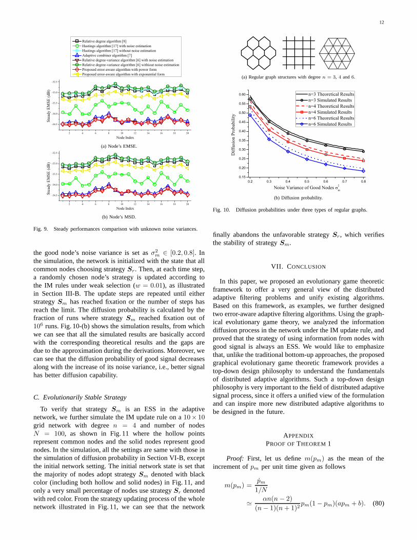
algorithm performs the best. The proposed algorithm withexponential form performs better than the relative degreealgorithm. With the power form fitness, the proposed algorithmcan achieve similar performance, if not better than, com-pared with adaptive combiner algorithm, and both algorithmsperforms better than all other algorithms except the relativedegree-variance algorithm. However, as discussed in Section 2,the relative degree-variance algorithm requires noise varianceinformation of each node, while our proposed algorithm doesnot. Fig. 7 shows the corresponding steady-state performancesof each node for six kinds of distributed adaptive filteringalgorithms in terms of EMSE and MSD. Since the steady-stateresult is for each node, besides averaging over500 independentrunnings, we average at each node over100 time slots afterthe convergence. We can see that the comparison results ofsteady-state performances are similar to those of the transientperformances.

In the second comparison, we assume that the noise varianceof each node is unknown, but can be estimated by the methodproposed in [17]. Fig. 8 and Fig. 9 show the transient andsteady-state performances for six kinds of algorithms in termsof EMSE and MSD under similar convergence rate. Sincethe noise variance estimation requires additional complexity,we also simulate the Hastings and relative degree-variancealgorithms without variance estimation for fair comparison,where the noise variance is set as the network average vari-ance, which is assumed to be prior information. Comparingwith Fig. 7, we can see that when the noise variance informa-tion is not available, the performance degradation of relativedegree-variance algorithm is significant, about 0.5dB (12%more error) even with noise variance estimation, while theperformance of Hastings algorithm degrades only a little sinceit relies less on the noise variance information. From Fig. 8-(b),

0 100 200 300 400 500 600 700 800 900 1000

-35

-30

-25

-20

-15

-10

-5

0

5

958 960 962 964 966 968 970 972 974 976

-34.6

-34.4

-34.2

-34.0

-33.8

-33.6

-33.4

-33.2

-33.0

-32.8

Relative degree algorithm [8] Hasting algorithm [17] with noise estimation Hasting algorithm [17] without noise estimation Adaptive combiner algorithm [7] Relative degree-variance algorithm [6] with noise estimation Relative degree-variance algorithm [6] withiout noise estimation Proposed error-aware algorithm with power form Proposed error-aware algorithm with exponential form

Tran

sien

t net

wor

k EM

SE (d

B)

Time Index

(a) Network EMSE.

0 100 200 300 400 500 600 700 800 900 1000

-35

-30

-25

-20

-15

-10

-5

0

5

978 980 982 984 986 988 990 992 994 996 998-34.6

-34.4

-34.2

-34.0

-33.8

-33.6

-33.4

-33.2

-33.0

-32.8

Relative degree algorithm [8] Hasting algorithm [17] with noise estimation Hasting algorithm [17] without noise estimation Adaptive combiner algorithm [7] Relative degree-variance algorithm [6] with noise estimation Relative degree-variance algorithm [6] withiout noise estimation Proposed error-aware algorithm with power form Proposed error-aware algorithm with exponential form

Tran

sien

t net

wor

k M

SD (d

B)

Time Index

(b) Network MSD.

Fig. 8. Transient performances comparison with unknown noise variances.

we can clearly see that when the variance estimation method isnot adopted, our proposed algorithm with power form achievesthe best performance. When the variance estimation methodis adopted, the performances of our proposed algorithm withpower form, the relative degree-variance and the adaptivecombiner algorithm are similar, all of which perform betterthan other algorithms. Nevertheless, the complexity of bothrelative degree-variance algorithm with variance estimationand the adaptive combiner algorithm are higher than thatof our proposed algorithm with power form. Such resultsimmediately show the advantage of the proposed generalframework. We should notice that more algorithms with betterperformances under certain criteria can be designed basedon the proposed framework by choosing more proper fitnessfunctions.

B. Diffusion Probability

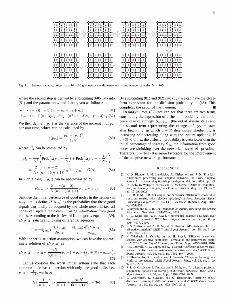
In this subsection, we develop simulation to verify thediffusion probability analysis in Section IV. For the simulationsetup, three types of regular graphs are generated with degreen = 3, 4 and6, respectively, as shown in Fig. 10-(a). All thesethree types of graphs are withN = 100 nodes, where eachnode’s trace of regressor covariance is set to be Tr(Ru) = 10,the common nodes’s noise variance is set asσ2

r = 1.5 and

12

2 4 6 8 10 12 14 16 18 20

-34.5

-34.0

-33.5

-33.0

-32.5

Relative degree algorithm [8] Hastings algorithm [17] with noise estimation Hastings algorithm [17] without noise estimation Adaptive combiner algorithm [7] Relative degree-variance algorithm [6] with noise estimation Relative degree-variance algorithm [6] withiout noise estimation Proposed error-aware algorithm with power form Proposed error-aware algorithm with exponential form

Stea

dy E

MSE

(dB

)

Node Index

(a) Node’s EMSE.

2 4 6 8 10 12 14 16 18 20

-34.5

-34.0

-33.5

-33.0

-32.5

Stea

dy E

MSE

(dB

)

Node Index

(b) Node’s MSD.

Fig. 9. Steady performances comparison with unknown noise variances.

the good node’s noise variance is set asσ2m ∈ [0.2, 0.8]. In

the simulation, the network is initialized with the state that allcommon nodes choosing strategySr. Then, at each time step,a randomly chosen node’s strategy is updated according tothe IM rules under weak selection (w = 0.01), as illustratedin Section III-B. The update steps are repeated until eitherstrategySm has reached fixation or the number of steps hasreach the limit. The diffusion probability is calculated bythefraction of runs where strategySm reached fixation out of106 runs. Fig. 10-(b) shows the simulation results, from whichwe can see that all the simulated results are basically accordwith the corresponding theoretical results and the gaps aredue to the approximation during the derivations. Moreover,wecan see that the diffusion probability of good signal decreasesalong with the increase of its noise variance, i.e., better signalhas better diffusion capability.

C. Evolutionarily Stable Strategy

To verify that strategySm is an ESS in the adaptivenetwork, we further simulate the IM update rule on a10× 10grid network with degreen = 4 and number of nodesN = 100, as shown in Fig. 11 where the hollow pointsrepresent common nodes and the solid nodes represent goodnodes. In the simulation, all the settings are same with those inthe simulation of diffusion probability in Section VI-B, exceptthe initial network setting. The initial network state is set thatthe majority of nodes adopt strategySm denoted with blackcolor (including both hollow and solid nodes) in Fig. 11, andonly a very small percentage of nodes use strategySr denotedwith red color. From the strategy updating process of the wholenetwork illustrated in Fig. 11, we can see that the network

(a) Regular graph structures with degreen = 3, 4 and6.

0.2 0.3 0.4 0.5 0.6 0.7 0.80.15

0.20

0.25

0.30

0.35

0.40

0.45

0.50

0.55

0.60

Diff

usio

n Pr

obab

ility

Noise Variance of Good Nodes 2m

n=3 Theoretical Results n=3 Simulated Results n=4 Theoretical Results n=4 Simulated Results n=6 Theoretical Results n=6 Simulated Results

(b) Diffusion probability.

Fig. 10. Diffusion probabilities under three types of regular graphs.

finally abandons the unfavorable strategySr, which verifiesthe stability of strategySm.

VII. C ONCLUSION

In this paper, we proposed an evolutionary game theoreticframework to offer a very general view of the distributedadaptive filtering problems and unify existing algorithms.Based on this framework, as examples, we further designedtwo error-aware adaptive filtering algorithms. Using the graph-ical evolutionary game theory, we analyzed the informationdiffusion process in the network under the IM update rule, andproved that the strategy of using information from nodes withgood signal is always an ESS. We would like to emphasizethat, unlike the traditional bottom-up approaches, the proposedgraphical evolutionary game theoretic framework providesatop-down design philosophy to understand the fundamentalsof distributed adaptive algorithms. Such a top-down designphilosophy is very important to the field of distributed adaptivesignal process, since it offers a unified view of the formulationand can inspire more new distributed adaptive algorithms tobe designed in the future.

APPENDIX

PROOF OFTHEOREM 1

Proof: First, let us definem(pm) as the mean of theincrement ofpm per unit time given as follows

m(pm) =pm1/N

≃ αn(n− 2)

(n− 1)(n+ 1)2pm(1− pm)(apm + b). (80)

13

Fig. 11. Strategy updating process in a10× 10 grid network with degreen = 4 and number of nodesN = 100.

where the second step is derived by substituting (60)-(64) into(51) and the parametersa andb are given as follows:

a= (n− 2)(n+ 3)(u1 − u2 − u3 + u4), (81)

b= −(n−1)(n+3)u1−3u2+(n2+n−3)u3+(n+3)u4.(82)

We then definev(pm) as the variance of the increment ofpmper unit time, which can be calculated by

v(pm) =˙p2m − (pm)2

1/N, (83)

where ˙p2m can be computed by

˙p2m =1

N2

(

Prob(

∆pm =1

N

)

+ Prob(

∆pm = − 1

N

)

)

=2

N2

n(n− 2)

(n− 1)(n+ 1)pm(1 − pm) +O(α). (84)

In such a case,v(pm) can be approximated by

v(pm) ≃ 2

N

n(n− 2)

(n− 1)(n+ 1)pm(1− pm). (85)

Suppose the initial percentage of good nodes in the network ispm0. Let us defineH(pm0) as the probability that these goodsignals can finally be adopted by the whole network, i.e., allnodes can update their ownw using information from goodnodes. According to the backward Kolmogorov equation [39],H(pm0) satisfies following differential equation

0 = m(pm0)dH(pm0)

dpm0+

v(pm0)

2

d2H(pm0)

dp2m0

. (86)

With the weak selection assumption, we can have the approx-imate solution ofH(pm0) as

H(pm0) = pm0 +αN

6(n+ 1)pm0(1− pm0)

(

(a+3b)+ apm0

)

.

(87)Let us consider the worst initial system state that each

common node has connection with only one good node, i,e.,pm0 = 1

n+1 , we have

H

(

1

n+ 1

)

≃ 1

n+ 1+

αnN

6(n+ 1)3(a+ 3b). (88)

By substituting (81) and (82) into (88), we can have the close-form expression for the diffusion probability in (65). Thiscompletes the proof of the theorem.

Remark: From (87), we can see that there are two termsconstituting the expression of diffusion probability: theinitialpercentage of strategySm, pm0 (the initial system state) andthe second term representing the changes of system stateafter beginning, in whicha + 3b determines whetherpm isincreasing or decreasing along with the system updating. Ifa+3b < 0, i.e., the diffusion probability is even lower than theinitial percentage of strategySm, the information from goodnodes are shrinking over the network, instead of spreading.Therefore,a+ 3b > 0 is more favorable for the improvementof the adaptive network performance.

REFERENCES

[1] V. D. Blondel, J. M. Hendrickx, A. Olshevsky, and J. N. Tsitsiklis,“Distributed processing over adaptive networks,” inProc. AdaptiveSensor Array Processing Workshop, Lexington, MA, Jun. 2006, pp. 1–3.

[2] D. Li, K. D. Wong, Y. H. Hu, and A. M. Sayed, “Detection, classifica-tion, and tracking of targets,”IEEE Signal Process. Mag., vol. 19, no. 2,pp. 17–29, 2002.

[3] F. C. R. Jr, M. L. R. de Campos, and S. Werner, “Distributedcooperativespectrum sensing with selective updating,” inProc. European SignalProcessing Conference (EUSIPCO), Bucharest, Romania, Aug. 2012,pp. 474–478.

[4] S. Haykin and K. J. R. Liu,Handbook on Array Processing and SensorNetworks. New York: IEEE-Wiley, 2009.

[5] C. G. Lopes and A. H. Sayed, “Incremental adaptive strategies overdistributed networks,”IEEE Trans. Signal Process., vol. 55, no. 8, pp.4064–4077, 2007.

[6] F. S. Cattivelli and A. H. Sayed, “Diffusion LMS strategies for dis-tributed estimation,”IEEE Trans. Signal Process., vol. 58, no. 3, pp.1035–1048, 2010.

[7] N. Takahashi, I. Yamada, and A. H. Sayed, “Diffusion least-meansquares with adaptive combiners: Formulation and performance analy-sis,” IEEE Trans. Signal Process., vol. 58, no. 9, pp. 4795–4810, 2010.

[8] F. S. Cattivelli, C. G. Lopes, and A. H. Sayed, “Diffusionrecursive least-squares for distributed etimation over adaptive networks,” IEEE Trans.Signal Process., vol. 56, no. 5, pp. 1865–1877, 2008.

[9] S. Theodoridis, K. Slavakis, and I. Yamada, “Adaptive learning in aworld of projections,”IEEE Signal Process. Mag., vol. 28, no. 1, pp.97–123, 2011.

[10] R. L. G. Cavalcante, I. Yamada, and B. Mulgrew, “An adaptive projectedsubgradient approach to learning in diffusion networks,”IEEE Trans.Signal Process., vol. 57, no. 7, pp. 2762–2774, 2009.

[11] S. Chouvardas, K. Slavakis, and S. Theodoridis, “Adaptive robustdistributed learning in diffusion sensor networks,”IEEE Trans. SignalProcess., vol. 59, no. 10, pp. 4692–4707, 2011.

14

[12] S.-Y. Tu and A. H. Sayed, “Mobile adaptive networks,”IEEE J. Sel.Topics Signal Process., vol. 5, no. 4, pp. 649–664, 2011.

[13] V. D. Blondel, J. M. Hendrickx, A. Olshevsky, and J. N. Tsitsiklis,“Convergence in multiagent coordination, consensus, and flocking,” inProc. Joint 44th IEEE Conf. Decision Control Eur. Control Conf. (CDC-ECC), Seville, Spain, Dec. 2005, pp. 2996–3000.

[14] L. Xiao, S. Boyd, and S. Lall, “A scheme for robust distributed sensorfusion based on average consensus,” inProc. Information ProcessingSensor Networks (IPSN), Los Angeles, CA, Apr. 2005, pp. 63–70.

[15] D. S. Scherber and H. C. Papadopoulos, “Locally constructed algorithmsfor distributed computations in Ad Hoc networks,” inProc. InformationProcessing Sensor Networks (IPSN), Berkeley, CA, Apr. 2004, pp. 11–19.

[16] L. Xiao and S. Boyd, “Fast linear iterations for distributed averaging,”Syst. Control Lett., vol. 53, no. 1, pp. 65–78, 2004.

[17] X. Zhao and A. H. Sayed, “Performance limits for distributed estimationover LMS adaptive networks,”IEEE Trans. Signal Process., vol. 60,no. 10, pp. 5107–5124, 2012.

[18] J. M. Smith, Evolution and the theory of games. Cambridge, UK:Cambridege University Press, 1982.

[19] R. Cressman,Evolutionary Dynamics and Extensive Form Games.Cambridge, MA: MIT Press, 2003.

[20] Y. Chen, Y. Gao, and K. J. R. Liu, “An evolutionary game-theoreticapproach for image interpolation,” inProc. IEEE ICASSP, 2011, pp.989–992.

[21] K. J. R. Liu and B. Wang,Cognitive Radio Networking and Security:A Game Theoretical View. Cambridge University Press, 2010.

[22] B. Wang, Y. Wu, and K. J. R. Liu, “Game theory for cognitive radionetworks: An overview,”Computer Networks, vol. 54, no. 14, pp. 2537–2561, 2010.

[23] E. H. Watanabe, D. Menasche, E. Silva, and R. M. Leao, “Modelingresource sharing dynamics of VoIP users over a WLAN using a game-theoretic approach,” inProc. IEEE INFOCOM, 2008, pp. 915–923.

[24] B. Wang, K. J. R. Liu, and T. C. Clancy, “Evolutionary cooperativespectrum sensing game: how to collaborate?”IEEE Trans. Commun.,vol. 58, no. 3, pp. 890–900, 2010.

[25] Y. Chen, B. Wang, W. S. Lin, Y. Wu, and K. J. R. Liu, “Cooperativepeer-to-peer streaming: an evolutionary game-theoretic approach,”IEEETrans. Circuit Syst. Video Technol., vol. 20, no. 10, pp. 1346–1357, 2010.

[26] C. Jiang, Y. Chen, Y. Gao, and K. J. R. Liu, “Joint spectrum sensingand access evolutionary game in cognitive radio networks,”IEEE Trans.Wireless Commun., vol. 12, no. 5, pp. 2470–2483, 2013.

[27] R. Fisher,The Genetical Theory of Natural Selection. Clarendon Press,1930.

[28] E. Lieberman, C. Hauert, and M. A. Nowak, “Evolutionarydynamicson graphs,”Nature, vol. 433, pp. 312–316, 2005.

[29] P. Shakarian, P. Roos, and A. Johnson, “A review of evolutionary graphtheory with applications to game theory,”Biosystems, vol. 107, no. 2,pp. 66–80, 2012.

[30] M. A. Nowak and K. Sigmund, “Evolutionary dynamics of biologicalgames,”Science, vol. 303, pp. 793–799, 2004.

[31] H. Ohtsuki, M. A. Nowak, and J. M. Pacheco, “Breaking thesymme-try between interaction and replacement in evolutionary dynamics ongraphs,”Phys. Rev. Lett., vol. 98, no. 10, p. 108106, 2007.

[32] H. Ohtsukia and M. A. Nowak, “The replicator equation ongraphs,”J.Theor. Biol., vol. 243, pp. 86–97, 2006.

[33] X. Zhao and A. H. Sayed, “Clustering via diffusion adaptation overnetworks,” in Proc. International Workshop on Cognitive InformationProcessing, Spain, May. 2012, pp. 1–6.

[34] M. Slatkin, “Fixation probabilities and fixation timesin a subdividedpopulation,” J. Theor. Biol., vol. 35, no. 3, pp. 477–488, 1981.

[35] H. Ohtsuki, C. Hauert, E. Lieberman, and M. A. Nowak, “A simple rulefor the evolution of cooperation on graphs and social networks,” Nature,vol. 441, pp. 502–505, 2006.

[36] F. Fu, L. Wang, M. A. Nowak, and C. Hauert, “Evolutionarydynamicson graphs: Efficient method for weak selection,”Phys. Rev., vol. 79,no. 4, p. 046707, 2009.

[37] G. Wild and A. Traulsen, “The different limits of weak selection and theevolutionary dynamics of finite populations,”J. Theor. Biol., vol. 247,no. 2, pp. 382–390, 2007.

[38] H. Ohtsukia and M. A. Nowak, “Evolutionary stability ongraphs,”J.Theor. Biol., vol. 251, no. 4, pp. 698–707, 2008.

[39] W. J. Ewense,Mathematical population genetics: theoretical introduc-tion. Spinger, New York, 2004.

Chunxiao Jiang (S’09-M’13) received his B.S.degree in information engineering from Beijing Uni-versity of Aeronautics and Astronautics (BeihangUniversity) in 2008 and the Ph.D. degree from Ts-inghua University (THU), Beijing in 2013, both withthe highest honors. During 2011-2012, he visited theSignals and Information Group (SIG) at Departmentof Electrical & Computer Engineering (ECE) ofUniversity of Maryland (UMD), supported by ChinaScholarship Council (CSC) for one year.

Dr. Jiang is currently a research associate in ECEdepartment of UMD with Prof. K. J. Ray Liu, and also a post-doctor in EEdepartment of THU. His research interests include the applications of gametheory and queuing theory in wireless communication and networking andsocial networks.

Dr. Jiang received the Beijing Distinguished Graduated Student Award, Chi-nese National Fellowship and Tsinghua Outstanding Distinguished DoctoralDissertation in 2013.

Yan Chen (S’06-M’11) received the Bachelor’s de-gree from University of Science and Technology ofChina in 2004, the M. Phil degree from Hong KongUniversity of Science and Technology (HKUST)in 2007, and the Ph.D. degree from University ofMaryland College Park in 2011. From 2011 to2013, he is a Postdoctoral research associate in theDepartment of Electrical and Computer Engineeringat University of Maryland College Park.

Currently, he is a Principal Technologist at OriginWireless Communications. He is also affiliated with

Signal and Information Group of University of Maryland College Park. Hiscurrent research interests are in social learning and networking, behavioranalysis and mechanism design for network systems, multimedia signalprocessing and communication.

Dr. Chen received the University of Maryland Future FacultyFellowshipin 2010, Chinese Government Award for outstanding studentsabroad in2011, University of Maryland ECE Distinguished Dissertation FellowshipHonorable Mention in 2011, and was the Finalist of A. James Clark Schoolof Engineering Deans Doctoral Research Award in 2011.

K. J. Ray Liu (F’03) was named a DistinguishedScholar-Teacher of University of Maryland, CollegePark, in 2007, where he is Christine Kim EminentProfessor of Information Technology. He leads theMaryland Signals and Information Group conduct-ing research encompassing broad areas of signalprocessing and communications with recent focuson cooperative and cognitive communications, sociallearning and network science, information forensicsand security, and green information and communi-cations technology.

Dr. Liu is the recipient of numerous honors and awards including IEEESignal Processing Society Technical Achievement Award andDistinguishedLecturer. He also received various teaching and research recognitions fromUniversity of Maryland including university-level Invention of the YearAward; and Poole and Kent Senior Faculty Teaching Award, OutstandingFaculty Research Award, and Outstanding Faculty Service Award, all fromA. James Clark School of Engineering. An ISI Highly Cited Author, Dr. Liuis a Fellow of IEEE and AAAS.

Dr. Liu is President of IEEE Signal Processing Society wherehe has servedas Vice President – Publications and Board of Governor. He was the Editor-in-Chief of IEEE Signal Processing Magazine and the founding Editor-in-Chiefof EURASIP Journal on Advances in Signal Processing.