TI 2011-100/3 Tinbergen Institute Discussion Paper

Distortionary Company Car Taxation: Deadweight Losses through Increased Car Ownership

Jos N. van Ommeren* Eva Gutiérrez-i-Puigarnau

Faculty of Economics and Business Administration, VU University Amsterdam. * Tinbergen Institute

Tinbergen Institute is the graduate school and research institute in economics of Erasmus University Rotterdam, the University of Amsterdam and VU University Amsterdam. More TI discussion papers can be downloaded at http://www.tinbergen.nl Tinbergen Institute has two locations: Tinbergen Institute Amsterdam Gustav Mahlerplein 117 1082 MS Amsterdam The Netherlands Tel.: +31(0)20 525 1600 Tinbergen Institute Rotterdam Burg. Oudlaan 50 3062 PA Rotterdam The Netherlands Tel.: +31(0)10 408 8900 Fax: +31(0)10 408 9031

Duisenberg school of finance is a collaboration of the Dutch financial sector and universities, with the ambition to support innovative research and offer top quality academic education in core areas of finance.

DSF research papers can be downloaded at: http://www.dsf.nl/ Duisenberg school of finance Gustav Mahlerplein 117 1082 MS Amsterdam The Netherlands Tel.: +31(0)20 525 8579

Jos van Ommeren is affiliated to the Tinbergen Institute, Amsterdam, The Netherlands. This research has been supported financially by the Netherlands Organisation for Scientific Research (NWO).

DISTORTIONARY COMPANY CAR TAXATION:

DEADWEIGHT LOSSES THROUGH INCREASED CAR OWNERSHIP

Jos N. van Ommeren

VU University, Amsterdam, The Netherlands j.n.van.ommeren@vu.nl

Eva Gutiérrez-i-Puigarnau

VU University, Amsterdam, The Netherlands egutierrez@feweb.vu.nl

17/07/2011

Abstract

We analyse the effects of distortionary company car taxation through increased household car

ownership for the Netherlands. We use several identification strategies and demonstrate that

for about 20 percent of households company car possession increases car ownership. The

annual welfare loss of distortionary company taxation through increased car ownership is

generally rather small, maximally €120 per company car, and likely much less. However, for

policies that exempt households from paying tax on their company car, the annual deadweight

loss is likely higher.

Keywords: Fringe benefits; taxation; company car; JEL codes: D12; D61; J33; R41; R48

2

1. Introduction

The supply and demand for fringe benefits receive much attention in economic textbooks (e.g.

Ehrenberg and Smith, 2003). The effect of distortionary fringe benefits taxation receives

however little attention in the transport and urban economics literature. This is surprising,

because there are strong indications that fringe benefit taxation has a strong effect on transport

related fringe benefits. The main examples are employer free parking, which is a common

fringe benefit in the US (e.g., Shoup, 2005; van Ommeren and Wentink, 2012) and company

cars, which are cars that are provided by employers to employees for private usage. Company

cars are widespread over the whole of Europe: about 40 percent of new cars are company cars

(Copenhagen Economics, 2010). 1

The reason why company car taxation is distortionary in Europe is easy to understand.

In most European countries, the exact level of the tax depends mainly on the company car’s

purchase price, but usually not on its private use (Copenhagen Economics, 2010). Cars which

are provided to employees for private usage are taxed at a rather low rate so the households'

implicit price of using a company car (including tax) is far below its market price.2 In these

countries, the households' implicit price of a company car is usually between 20 to 50 below

its market price. Given such a large price advantage, it is not so surprising that company cars

are common in Europe. One potential justification for favourable company car taxation is that

these cars increase workers' productivity. However, this appears not to be a convincing

argument, because the large majority of the company cars are not, or hardly, used for business

purposes. For example, only 20 percent of workers in the Netherlands regularly use their

1 Company cars are usually new, used for a period of about 3 to 4 years, and then sold on the secondhand market. In Europe about 15 to 20% of two-adult households have access to a company car (Gutiérrez-i-Puigarnau and van Ommeren, 2011). 2 To give a concrete example, in the Netherlands maximally 24 percent of the company car’s purchase price is added to annual taxable income. However, the annual cost of such a car is about 40 percent of its purchase price. In the literature it is common to distinguish between the price of owning and the price of using a car. This difference is not essential here, because employers usually pay for the possession of the car (usually through a car lease) including insurance and taxes but also for its use including fuel consumption and repairs (Wuyts, 2009).

3

company car for business purposes (Gutiérrez-i-Puigarnau and van Ommeren, 2011).3 For

Belgium, similar numbers are reported: less than 10 percent (20 percent) of trips (of mileage)

with a company car are incurred for business purposes. Another interesting example is that 13

percent of lower level administrative staff, for whom productivity effects of company cars are

absent, receive a company car (De Borger and Wuyts, 2011). It is then not so hard to see that

in most European countries, taxation of company cars is far from optimal.

Distortionary company car taxation has several consequences for behaviour of

households. One expects that the reduced price of having a (company) car induces households

to demand a more expensive company car and travel more privately than they would

otherwise. In a recent paper, we have shown that these behavioural changes imply that company

car taxation is strongly distortionary and induces an annual welfare loss of about €350 to €700

per company car (see, Gutiérrez-i-Puigarnau and van Ommeren, 2011). Although such a

welfare loss is substantial, this estimate has been argued to be still an underestimate because it

ignores other behavioural changes. In particular, it is plausible that due to the company cars'

reduced price, households will also increase car ownership, so the number of cars in the

household will increase. This will be the focus of the current paper.

There are several indications that increases in car ownership due to company car

taxation is quantitatively important. First, about 25 percent of Belgian employees with a

company car state that they would reduce household car ownership when they would not

receive a company car (De Borger and Wuyts, 2011). Second, the household car ownership

studies by Whelan et al. (2001) and Han (2001) suggest that the presence of a company car in

the household increases car ownership.4 However, these two studies ignore a range of

3 However, even when a worker uses a company car for business purposes then this does not necessarily imply that the worker is more productive, because most workers use a car for commuting. So when not offered a company car, they may use a private car for business purposes (and receive reimbursement from their employer for the marginal costs related to business trips). 4 Empirical car ownership studies, which aim to explain the number of cars in the household are abundant in the transportation literature (see e.g., Kumar and Rao, 2006; Dargay and Gateley, 1999;

4

statistical and economic issues. In particular, they do not take into account endogeneity issues

and control only for a few explanatory variables. Furthermore, they do not attempt to derive

the welfare effects of distortionary taxation. The present work deals with these issues.

Third, fuel price and car price elasticities of car ownership in the transport literature are

suggestive. Note that some of these studies measure car ownership at the individual (rather

than the household) level, so interpretation of the elasticities for our purpose is not

straightforward. We focus on long-run elasticities.5 Two meta-analyses using different studies

conclude that the long-run fuel price elasticity of ownership is around - 0.20 (Brons et al.,

2008; Goodwin et al., 2004). This suggests that the presence of a company car, which reduces

the fuel price toward zero, may increase the number of cars through free fuel only by, on

average, 14 percent ((log(2) - log (1)) × -0.20), as most company car owners receive free fuel

for private travel. The long-run car price ownership elasticity is estimated to be between - 0.1

and -0.5 (Ubbels, 2006; Goodwin et al., 2004; Dargay and Vythoulkas, 1999; Johansson and

Schipper, 1997), whereas the more elastic estimate is more common.6 If a company car is

offered to employees at an effective price that is 20 to 50 percent below the price in the car

market, as is common in Europe, then current studies suggest an increase in car ownership of

10 to 30 percent.

Company cars are predominantly taxed in Europe based on the company car’s purchase

price. We focus on the Netherlands where the implicit average price of a company car paid by

the household is about 30 percent below its market price (Gutiérrez-i-Puigarnau and van

Ommeren, 2011). The level of the company car tax does not depend on the extent of business

use. However, economic theory indicates that optimal fringe benefits taxation must not be

Holtzclaw, 1994). However, these studies ignore company cars, which is a major omission when applied to European countries. 5 We focus on the long-run, because it is then plausible that households fully adapt to changes in prices, similar to households that have a company car and are confronted with different prices. 6 It is suggested in the literature that most of the reported car price elasticities of ownership are downward biased, because they omit car quality measures, so the price elasticities are plausible somewhat larger.

5

based on the company car’s purchase price, but must be derived from the firm’s costs of

providing a company car, e.g. the leasing price, (and any compensation that a worker receives

for the marginal cost of business trips (e.g. fuel costs) must not be taxed), as is the current

practice in the US. However, the latter tax policy requires differentiation between business

and private kilometres for tax purposes, which entails higher monitoring costs for tax

authorities. Similarly, in some European countries, the level of company car tax depends on

the combination of company car's private and business use (Copenhagen Economics, 2010).7

Rather obviously, company car possession only increases household car ownership if

there is any demand for more than one car in the household. So, for single-person households

who own a private car, car ownership is unlikely to increase when they receive a company

car, as single-person households seldom desire more than one car. However, in two-adult

households with one private car, car ownership is more likely to increase, because there is

usually a latent demand for a second car. One expects then that an increase in car ownership is

particularly likely to happen, if the company car is an imperfect substitute for the private car.

For this reason, we identify the effect of distortionary company car taxation on car

ownership for two-adult households in the Netherlands. We do so by estimating the effect of

company car possession (which captures a car price reduction due to company car taxation)

on the decision to have more than one car for a sample of two-adult households who have at

least one car. Households with cars have usually little reason to refuse a company car, which

will be cheaper than their private car, as a part of their employment contract. This implies that

whether a household has a company car is mainly determined by the firm’s company car

policy and therefore by the household's members specific occupations (Tillema et al., 2008).

This strongly reduces the likelihood that company car possession is endogenous with regard

7 For example, in the UK, until recently, the tax level decreased strongly with business mileage.

6

to household car ownership. Nevertheless, as endogeneity cannot be excluded, we will mainly

focus on estimates where endogeneity is addressed.

In the next section, we discuss the theoretical setting. The remainder of the paper is

structured as follows: section 3 provides information on the data used, introduces the different

statistical models and presents the empirical results. Sections 4 and 5 examine the welfare

analyses. Section 6 concludes.

2. Theory

To determine the welfare effects of the tax treatment of company cars, we use a standard

household model that includes wages and identical cars (see Gutiérrez-i-Puigarnau and van

Ommeren, 2011, who allow for heterogeneous cars). We assume that the labour market is

perfectly competitive and the car market is perfectly competitive with a horizontal supply

curve.8 The car price is denoted by p. For simplicity, we assume that a household does not

demand more than two cars. When the household owns a car, the indicator z equals one,

otherwise it is zero; when the household owns also another car, the indicator x equals one,

otherwise it is zero. There is only one other composite good y. Labour income is denoted by

m and τ denotes the marginal income tax. The household maximizes utility U(z,x,y) given a

household income constraint: p(z +x) + y = m(1− τ), where the price of y is standardized to

one. Let us now assume that z equals 1. This is in line with our data, as (almost) all

households have at least one car.

Given these assumptions, the household utility function may be written as a standard

two-good utility function U(x,y) given the constraint px + y = m(1− τ) −p. The function

x(p,m(1− τ) − p) is then the Marshallian car demand function for the second car. In case the

8 The results by Zax (1988) suggest that monopsony has little effect on the welfare effects of fringe benefits taxation, so this issue will be ignored. The car market is described by the partial-equilibrium perfectly competitive model, where costs and pre-tax prices are not affected by the tax distortion. We abstract from market power by car suppliers (see Berry et al., 1995; Verboven, 1996).

7

household has two private cars (and has no demand for a third car), then company car

possession will have no effect on car ownership. We will therefore from now on focus on a

household that has one private car (rather than two), so x = 0. For this household holds that

U(0, m(1− τ) − p) exceeds U(1, m(1− τ) − 2p).

Suppose that the tax authorities allow firms to offer one company car as a fringe

benefit. So we now focus on the firm that offers a company car and gross income mc. The tax

system values the company car at a price H, where H < p. In a competitive labour market, a

firm chooses to offer a company car when total labour costs will fall, so mc+p ≤ m and the

utility of the household must remain the same implying that

c cU(0, m - (m +H)) U(0, m(1- ) -p) . A (textbook) non-distortionary tax treatment of company

cars requires that H = p and mc+p = m. The latter equality implies that labour expenses of the

firm, and therefore its profit, do not depend on company car taxation and that company car

taxation only distorts the car market.

It is reasonable to assume that company cars and private cars are either perfect

substitutes, imperfect substitutes9 or unrelated goods. For convenience, we will focus on the

case that these cars are either perfect substitutes or unrelated goods. Let us suppose first that

the company car is a perfect substitute for the private car. As the company car is cheaper than

the private car the household will always accept the company car and then decide whether or

not to have a private car. The function , 1c cx p m H is then the household's

Marshallian demand function for the second car conditional on receiving a company car.

When a household receives a company car at a reduced price, there may be an income and a

substitution effect on car demand. The income effect is likely small, because firms that offer

company cars reduce wages at the same time. Given a competitive labour market (or a

9 When the type of car received as a company car is not the preferred choice of the household then the company car is an imperfect substitute. This was common in the 90s when the lease market for cars was not well developed in Europe, so company cars were usually owned by the employer without considering the preferences of households.

8

quasilinear utility function), there is even no income effect of receiving a car at a lower price.

So, the price effect of company car taxation on household car ownership must be interpreted

as the compensated price effect. So, assuming that there is no income effect of receiving a

company car, this implies that xc = x. Hence, given the assumption that the company car is a

perfect substitute, company car taxation does not induce welfare losses through changes in

car ownership.

Let us now suppose that company and private cars are unrelated goods. This may be due

to a number of reasons. One reason is that other members of the household are not allowed to

drive the company car due to car insurance reasons (this is, for example, standard in the UK,

but not in the Netherlands). Another reason might be, applicable in the Netherlands after

2002, that the tax paid on receiving a company car depends on the number of kilometres

driven privately (discussed in detail later on). It may also be case the company car is used for

commuting, and other members of the household need a car for commuting.

In the case that company cars and private cars are unrelated goods, the household

decides to accept the offer of the company car, its utility is equal to c cU(1, m - (m +H)- p)

otherwise it is equal to U(0, m(1− τ) − p). Given mc+p = m, one can show that p – τ(p − H)

can be interpreted as the household's effective price for the company car and – τ(p − H) as the

company car tax advantage. The function , 1c cx p p H m p is then the

household's Marshallian demand function for the second car conditional on receiving a

company car. We aim to estimate the demand for a second car, conditional on receiving, or

not receiving, a company car, which is the basis of our welfare analysis. We then focus on the

difference in the demand for a second car for households with or without a company car, so

we focus on the difference between x and xc.

Given estimates of the demand function, and the assumption that the company car is

either a perfect substitute or unrelated to private car, it is straightforward to determine the

9

welfare effect of the tax treatment of the company car. In our estimates, we control for

income. When income is given, consumer’s surplus is a reasonable approximation of welfare.

We assume that the demand for the second car is a linear function of its price, so the reduction

in consumer surplus and therefore welfare, can be calculated using the rule of half.10 The

change in demand for a second car due to company car procession is then equal to the change

in the probability of having two cars due to receiving a company car. We denote the change in

this probability by P. Assuming that company car possession implies a subsidy equal to Ω, the

reduction in consumer surplus through increased car demand is equal to 0.5 P Ω. This

calculation of the welfare effect in this way is rather rough. First, we assume that company

cars are either a complete substitute or unrelated to private cars and, second, we ignore that

demand for a second car is a discrete demand. However, our welfare estimates are a

reasonable estimate of the order of magnitude of the incurred deadweight loss.

Distortionary company car taxation may not only increase car ownership but may also

increase the demand for commuting (see Gutiérrez-i-Puigarnau and van Ommeren, 2011). If

we assume that household utility is additive-separable in commuting and car ownership, then

we may examine the distortionary effect of company car taxation on car ownership ignoring

its effect on commuting distance. As this assumption may not hold, we will also report

estimates controlling for commuting distance. Another issue is that we ignore that some

company cars are productive and that the car market is distorted by purchase and user taxation

which may result in an overestimate of the welfare loss caused by company car taxation. We

address both issues later on by making assumptions on the proportion of company cars that

are productive and by taking other distortionary taxation into account.

10 We ignore here that a car is a discrete good. Assuming a discrete demand function, welfare analysis is possible using the methodology proposed by Small and Rosen (1981).

10

3. Car ownership demand analysis

3.1. The data

We aim to estimate the effect of company car possession on car demand in the household. Our

empirical analysis is based on information from the annual 1995–2009 DNB (Dutch Central

Bank) survey, which is a household panel survey. As there are only a few households with

more than two cars, we model car demand as a discrete choice between one or more than one

car. In all analyses, we employ samples of two-adult households that possess at least one car

(and which contain at least one full-time employed adult).11 To facilitate interpretation of our

results, we also exclude a few observations referring to households that have two company

cars. Furthermore, we exclude observations when the head of the household is self-employed

or relevant information is missing.12 In total we have 7,429 observations for 2,644

households.

Descriptive statistics show that 14.7 percent of the households own a company car

and 20 percent of the households own (at least) two cars. Bivariate statistics suggest a strong

relationship between company car possession and car ownership: 45 percent of households

with a company car have (at least) two cars, whereas this applies to 15 percent of households

without a company car. This suggests that company car possession increases household car

ownership by 30 percent.

In the multivariate analyses, we will use several identification strategies. One of our

identification strategies implies a household fixed-effects approach, so this identification

strategy relies on changes over time in household company car possession and household car

11 Given an unconstrained choice of the data the statistical analysis becomes cumbersome, as the presence of a company car is then endogenous, as it indicates the presence of at least one car. This selection is not problematic, because merely 6% of households do not own a car and these households seldom belong to the social group of households who receive a company car offer. 12 For most variables, information is almost complete. The main exception is household income which is missing for about one third of the observations. Including these observations, and using a control dummy variable to control for missing income, generates almost identical effects.

11

ownership. It appears that there is sufficient time variation in both variables: we observe 360

household changes in car ownership and 112 household changes in company car possession.

3.2. Empirical analysis

In our empirical application, car demand is captured by a dichotomous variable which

measures whether the number of cars exceeds one. To estimate the effect of car ownership on

car demand, we rely on linear probability models (rather than discrete choice models).13 We

estimate specifications with ordinary regression (OLS), with instrumental variables (IV) as

well as with household fixed effects (FE). We use a range of relevant time-varying control

variables, including number of children, household income (in log), residence ownership, five

dummy indicators which capture population density in the municipality of residence, head

employment status (permanently or temporarily employed), partners employment

employment status (employed or non-employed). Further, we control for year and residence

region dummies. When we do not control for household fixed effects, we also control for

head’s age, gender and education (which are not identified given year dummies and

household fixed effects). For now, we assume that the effect of company car possession is a

constant and the same for all households, so it does not depend on calendar time or household

characteristics.

Our main finding is that the possession of a company car strongly increases the number

of cars in the household. This holds for all identification strategies (see Table 1). For the OLS

estimates without any control variables except for year dummies, the effect of company car on

car ownership is 0.29 (and highly statistically significant with a standard error of less than

13 The main reason is that in one of our estimation strategies we use household fixed effects. Given a logit specification with fixed effects, parameters can be consistently estimated using a conditional likelihood procedure, but, the marginal effects of explanatory variables, in which we are interested, are then not defined. Another issue is that for fixed effects logit models, parameters are entirely identified using households that change car ownership. This is problematic, because it is plausible that those households that change ownership are on average more sensitive to changes in prices of cars than other households.

12

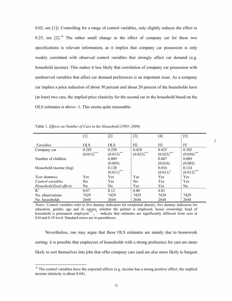
0.02, see [1]). Controlling for a range of control variables, only slightly reduces the effect to

0.25, see [2].14 The rather small change in the effect of company car for these two

specifications is relevant information, as it implies that company car possession is only

weakly correlated with observed control variables that strongly affect car demand (e.g.

household income). This makes it less likely that correlation of company car possession with

unobserved variables that affect car demand preferences is an important issue. As a company

car implies a price reduction of about 30 percent and about 20 percent of the households have

(at least) two cars, the implied price elasticity for the second car in the household based on the

OLS estimates is above -1. This seems quite reasonable.

Table 1. Effects on Number of Cars in the Household (1995–2009)

[1] [2] [3] [4] [5] | Variables OLS OLS FE FE IVCompany car 0.285

(0.015)*** 0.250 (0.013)***

0.428 (0.023)***

0.425 (0.023)***

0.302 (0.056)***

Number of children

0.009 (0.005)

0.007 (0.010)

0.009 (0.005)

Household income (log)

0.128 (0.011)***

0.016 (0.011)*

0.124 (0.012)***

Year dummies Yes Yes Yes Yes YesControl variables No Yes No Yes Yes Household fixed effects No No Yes Yes No R2 0.07 0.12 0.80 0.81 No. observations 7429 7429 7429 7429 7429 No. households 2644 2644 2644 2644 2644 Notes: Control variables refer to five dummy indicators for residential density, five dummy indicators for education, gender, age and its square, whether the partner is employed, house ownership, head of household is permanent employed.***, *– indicate that estimates are significantly different from zero at 0.01and 0.10 level. Standard errors are in parentheses.

Nevertheless, one may argue that these OLS estimates are mainly due to housework

sorting: it is possible that employees of households with a strong preference for cars are more

likely to sort themselves into jobs that offer company cars (and are also more likely to bargain

14 The control variables have the expected effects (e.g. income has a strong positive effect; the implied income elasticity is about 0.64).

13

for this fringe benefit conditional on the specific job), which suggests that the OLS estimate is

biased and is an overestimate.

So we have estimated models with household fixed effects, which control for time-

invariant preferences for cars. We now find that the effect of company car is not lower, but

substantially higher and equal to 0.43 (see [3]). This finding is robust to the inclusion of

control variables (see [4]). Our results that the fixed effects estimate is higher than the OLS

estimate is plausible, because fixed effects estimates must be interpreted as short-run

estimates. Because not all households who receive a company car will immediately sell their

private car, it is plausible that the short-run effect exceeds the long-run effect.15

By controlling for household effects, we avoid arguments that households with strong

preferences for cars sort themselves into jobs with company cars so that the effect of company

car is due to time-invariant unobserved car preferences of households. Further, we control for

many time-varying demand variables including income and the number of children. However,

one may argue that the presence of time-varying unobserved demand variables creates an

estimation bias (e.g. a sudden increase in the demand for the second car induces employees

without a company car to sort themselves into other jobs that offer company cars).

A relevant example which comes to mind is that company cars are offered to workers

who do not use a car for commuting and that these cars are offered by organisations that are

difficult to reach other than by car. In this case, one may argue that the effect we have

identified above is not merely due to reduced price for the company car but also due to the

length of the commute, so we have an overestimate. To address this point, we have re-

estimated the models adding a control for the head’s commuting distance (we have

information about this variable after the year 2001). We find that the effect of company car 15 Households who receive a company car may not immediately sell their private car for several reasons: first, it takes time to find a buyer; second, some households may be uncertain of the expected employment duration and company car possession may be considered temporary; third, some households might be uncertain of the benefits of having more than one car and keep the private car for a short period to experience the advantage of having two cars.

14

remains the same (see Table 2).16 Furthermore, we have estimated IV models (with and

without controlling for commuting distance) using as an instrument whether or not the

households head is employed by a public organisation.17

Table 2. Effects on Number of Cars in the Household controlling for commuting distance (2001–2009) [1] [2] Variables OLS IV Company car 0.312

(0.056)*** 0.261 (0.096)***

Commuting distance (log) 0.035 0.040 (0.008)*** (0.011)*** Number of children 0.017

(0.005)* 0.017 (0.008)*

Household income (log) 0.119 (0.012)***

0.110 (0.020)***

Year dummies Yes Yes Control variables Yes Yes Household fixed effects No No R2 0.13 No. observations 2397 2397 No. households 840 840 Notes: see Table 1.

So the assumption we make is that, given household income and other observed demand

indicators (e.g. number of children, commuting distance), the demand for cars is exogenous

with respect to whether the head of the household is employed by a public organisation. In the

specification we distinguish between two types of public organisations (civil servants and

others, such as hospitals). These instruments are strong with an F-test of 170. A standard

overidentification test does not reject the instruments (however, as the instruments are similar

16 In this specification we ignore that commuting distance is potentially endogenous. We are not able to control for other private kilometres travelled as it is unobserved in this dataset. However, this is less relevant as private travel (excluding commuting) is roughly the same for households with and without a company car (Gutiérrez-i-Puigarnau and van Ommeren, 2011). 17 In the dataset, we do not have specific information about the type of industry, but we have information about the names of the pension fund of the current employer. In this way, we are able to derive the type of industry in an unusual way. So, we are able to distinguish between employees that work in public organisations (government, universities) or private organisations. We are also able to distinguish between broad categories of private organisations. This information is later on used in the sensitivity analysis.

15

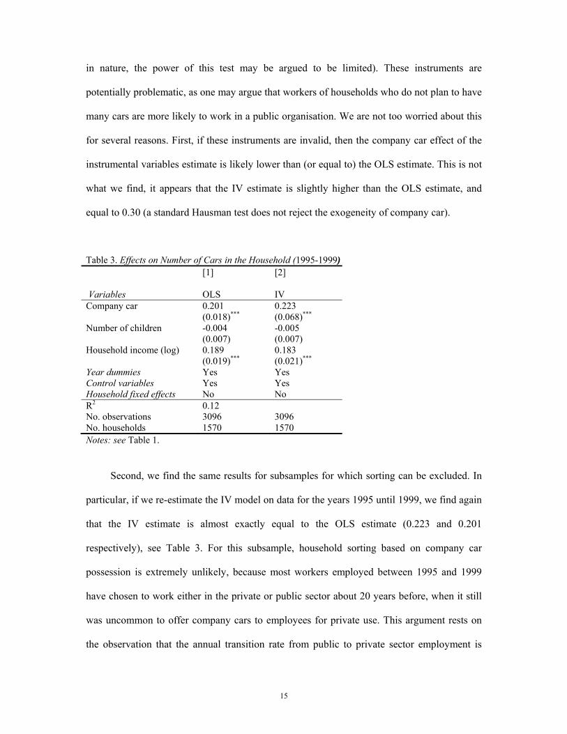
in nature, the power of this test may be argued to be limited). These instruments are

potentially problematic, as one may argue that workers of households who do not plan to have

many cars are more likely to work in a public organisation. We are not too worried about this

for several reasons. First, if these instruments are invalid, then the company car effect of the

instrumental variables estimate is likely lower than (or equal to) the OLS estimate. This is not

what we find, it appears that the IV estimate is slightly higher than the OLS estimate, and

equal to 0.30 (a standard Hausman test does not reject the exogeneity of company car).

Table 3. Effects on Number of Cars in the Household (1995-1999) [1] [2] Variables OLS IV Company car 0.201

(0.018)*** 0.223 (0.068)***

Number of children -0.004 (0.007)

-0.005 (0.007)

Household income (log) 0.189 (0.019)***

0.183 (0.021)***

Year dummies Yes Yes Control variables Yes Yes Household fixed effects No No R2 0.12 No. observations 3096 3096 No. households 1570 1570 Notes: see Table 1.

Second, we find the same results for subsamples for which sorting can be excluded. In

particular, if we re-estimate the IV model on data for the years 1995 until 1999, we find again

that the IV estimate is almost exactly equal to the OLS estimate (0.223 and 0.201

respectively), see Table 3. For this subsample, household sorting based on company car

possession is extremely unlikely, because most workers employed between 1995 and 1999

have chosen to work either in the private or public sector about 20 years before, when it still

was uncommon to offer company cars to employees for private use. This argument rests on

the observation that the annual transition rate from public to private sector employment is

16

close to zero for our sample (it is 0.0087) and the average worker with a company car in the

period between 1995 and 1999 is 46 years, so this worker started to work in the beginning of

the 70s.

Third, as an informal way to test the validity of the instruments, we have included both

instruments directly into the OLS regression, see similarly Arzaghi and Henderson (2008).

When company car possession is correlated with unobserved household characteristics, then

the instruments will absorb some of the bias of the company car. If the instruments are not

valid, the effect of company car should decline. Given this specification however, we find an

almost identical coefficient for company car compared to the first OLS estimate, suggesting

that our instruments are valid.18

Fourth, the instrument relies on the explicit assumption that type of sector does not

directly influence car demand, which is implemented by distinguishing between public and

private sector. Hence, one way to test for the validity of our public sector instruments is to

distinguish between different types of private sector (e.g. bank, retail) and use type of private

sector as a control variable in the IV approach. When we control for type of private

employment, we find exactly the same effect for company car, and, importantly, we do not

find any evidence that type of private sector has any direct effect on car ownership.19 In

particular, this suggests that our estimates are not driven by differences in workplace location

(as firms strongly differ in terms of location; for example, business services and industry are

typically located at different locations) and also not driven by differences in demand for

business trips (as firms strongly differ in their demand for business trips).

We conducted several additional analyses to evaluate the sensitivity of the reported

effect of company car possession on car demand. In particular, one may argue that the effect 18 It also appears that our instruments have no direct impact on car ownership conditional on including company car possession suggesting that any effect of sector is through company car possession. 19 As an informal test, we exclude company car in the OLS analysis, and find a strong effect of type of private sector which also implies that the effect of type of private sector is entirely through company car possession, supporting our assumption that public sector is a valid instrument.

17

of household income on car demand is non-linear, so we added the square (and also the cubic)

of net household income in log as controls, but find that the results remain the same.

We re-estimated the models by splitting the sample in low and high income households.

This is interesting because the marginal income tax is somewhat increasing in income and

price elasticities of demand may differ by income. We find roughly the same estimates for

both income groups. Finally, we estimated all models using a probit specification. In essence,

the average marginal effect given this specification is almost exactly equal to the marginal

effect of the linear specification. We will continue now on the assumption that the 0.20

estimate is the most accurate estimate. We emphasise that this is a conservative estimate

given the range of estimated coefficients. About 12 percent of all personal cars in the

economy are company cars, so the presence of company cars increases the overall number of

cars on the economy by about 2.4 percent. This seems a substantial number, but this number

is not indicative about the welfare effects of company car taxation.

4. Welfare effects through changes in car ownership

To examine the welfare effects of current company car taxation, we use market averages. The

additional annual expenditure on a car is about €4000. The tax advantage is assumed to be 30

percent. The annual loss of consumer surplus is then equal to 0.5*0.2*€4000*0.3 = €120.20

This is a useful estimate, but it is also useful to consider the plausible range of the deadweight

loss. For the households that do not pay any tax on the company car (those that do not drive

privately, except for commuting), the subsidy is about 0.5. Given the (conservative)

assumption that for these households the probability to increase car ownership is 0.2 (so it is

not higher for households that do not drive privately except for commuting), the annual 20 One objection to our analysis may be that employers that lease a large number of cars receive bulk discounts due to a reduction in transaction costs. Bulk discounts are typically less than 10%, but precise figures are unknown to us. If we assume that employers provide company cars at an average reduction of 5% (and that these reductions are not due to market power), then the welfare loss due to the tax distortion is overestimated by 5%.

18

welfare loss is at least €200 (0.5*0.2*€4000*0.5). For countries such as Belgium, where

households are exempted from paying tax on company cars, €200 seems the more plausible

welfare loss.

In the Netherlands, there are about 800,000 company cars. As explained in the

introduction some of these company cars may be productive, but previous studies indicate that

maximally 20 percent of the company cars are productive. Let us first assume that the effect

of company car on household car ownership does not depend on whether the company car is

productive. This implies that 600,000 company cars are used merely for private reasons.

Given a welfare loss of €120 per company car, the annual welfare loss of distortionary

company car taxation through increased household car ownership is about €70 million.

Clearly, the deadweight loss of distortionary company car taxation is sizeable. Nevertheless,

this loss is only 10 percent of the reported deadweight loss of company car taxation due to

increased expenditure on the company car as well as increased driving (Gutiérrez-i-Puigarnau

and van Ommeren, 2011). However, one may argue that the €70 million is still an

overestimate because company cars that are productive are less likely a substitute for a private

car (when a car is used for business reasons, it cannot be used by other members of the

household), implying that the annual welfare loss is maximally €70 million.

Our data allow us to examine the effects of policy changes. Company cars are taxed as a

fringe benefit when they are privately used. So, tax authorities have to define what private use

implies. For an increasing number of trips it turns out to be difficult to determine whether the

trip with the company car is for business or for private reasons. This is particularly the case

for business trips that originate from the employee's home. For this reason, after the year

2002, Dutch tax authorities have stipulated that all commuting trips were considered business

trips. This implies that if the company car is not used privately except for commuting, then it

is regarded as a non-taxable fringe benefit. This gives an incentive to households to use the

19

company car only for commuting, and to buy another private car which can be used for other

private trips (e.g. holidays). So, one expects that after 2002, company car possession has a

stronger effect on household car ownership than before.21

We find evidence of this in the OLS specification if we include the interaction of

company car with calendar year. The increased effect is statistically significant and about 0.08

(with a standard error of 0.03). However, given a households fixed effect specification, we do

not find any evidence: the effect is highly insignificant and the point estimate is even slightly

negative (-0.02). For the instrumental variable estimation procedure, we find a positive effect

of about 0.13, but it is not statistically significant (the standard error is 0.10). So, the different

approaches do not agree on whether this policy change has increased the distortionary effect

of company car taxation.

5. Welfare effects: sensitivity analyses

In our calculation of welfare effects, we assumed a world in which company car taxation is

the sole tax distortion in the economy. Car taxes entail taxes on purchase, use and fuel (e.g.,

Craft and Schmidt, 2005 and Bento et al., 2009). The aggregate revenues from these taxes are

considerably, so, in principle, they cannot be ignored. Arguably, fuel and user taxes may be

justified as second-best instruments to finance road maintenance costs and to address

congestion and other externalities associated with travel (Vickrey, 1963; Small and Bento,

2005; de Palma et al., 2006; Small and Verhoef, 2007). However, this is less plausible for

purchase taxes, which apply to new car purchases. The car purchase tax during our

observation period was 42.3 percent (for most cars). About 40 percent of the overall car

21 However, at the same time, the tax on company cars was slightly increased, which reduces the probability that a company car is offered by the firm, so the increase in welfare loss per company car may have been offset by a reduction in the number of company cars. Furthermore, employees have a strong incentive to cheat by declaring that the car is only used for commuting but not for other trips. Cheating households do not have an additional incentive to increase car ownership.According to the tax authorities, about 20% of households cheat.

20

expenses relate to fixed costs, so the purchase tax disadvantage in terms of overall car

expenses is 17 percent (0.40 × 0.423), which is substantially smaller than the tax advantage

obtained from the provision of a company car (about 30 percent). Therefore, our results are

qualitatively robust with respect to the presence of other distortionary car taxes. When the

purchase taxes are fully distortionary, the imputed subsidy is only 13 percent, but also the

estimated distortionary tax effect of company car possession on car ownership is presumably

much lower than 0.2. If we presume that the effect of car ownership given this smaller

subsidy is 0.1 then the annual deadweight loss per company car is only €30, which is

substantially less than the € 120 indicated above. However, purchase taxes may address a

number of negative car externalities, including accident externalities which increase in the

number of cars on the road, parking externalities (cars need space that is usually provided for

free) and congestion externalities in cities. Thus, purchase taxes are not fully distortionary.

When the purchase tax will be abolished (in 2016), €120 is the more accurate estimate of the

deadweight loss through increased car ownership.22

6. Conclusions

Economic theory is quite clear on how fringe benefits such as company cars should optimally

be taxed. In Europe, company cars are common, but the welfare effects of the current tax

system in Europe have hardly been analysed. We study the welfare effect of company car

taxation through increased household car ownership. We find that for the Netherlands for

about 20 percent of households, company car possession increases car ownership. Our results

22 Tax advantage given to company cars may (partially) compensate for the presence of distortionary purchase taxes on personal cars that are substantial in Europe. Since in most other European countries, purchase car taxes are lower than in the Netherlands, our conclusion that the tax system is distortionary regarding company cars can be generalized to other European countries. This conclusion may not hold in countries such as Denmark and Norway, where purchase taxes are 180% respectively 100% of the car’s purchase price. For these countries, it is possible that favourable company car taxation generates substantial welfare benefits as purchase taxes on personal cars can be argued to be too high in these countries, so that company car taxation corrects for the purchase tax distortion.

21

imply that the tax treatment of company cars induces an annual deadweight loss per company

car of maximally €120 due to increased car ownership. Our results suggest further that tax

authorities' definition of private travel has implications for welfare. When a commuting trip is

defined by tax authorities as a business trip, then this increases the incentive for households to

increase car ownership. So, for policies that exempt households from paying tax on their

company car by defining commuting trips as a business trips, the annual welfare loss may be

much higher than €120.

Allowing for productivity effects of company cars and the presence of other

distortionary taxation (e.g. purchase car taxation), the estimated total annual welfare loss due

to distortionary company car taxation through increased car ownership is rather moderate and

about €30 per car. This deadweight loss is only a small proportion (less than 10 percent) of

the welfare loss reported due to increased expenditure on the company car as well as due to

increases in car mileage (Gutiérrez-i-Puigarnau and van Ommeren, 2011). The result that the

deadweight loss consists mainly of a shift towards more expensive cars is consistent with a

literature that points out that car demand is rather price elastic (Bento et al., 2009), whereas

the demand for car ownership is more price inelastic (Small and Verhoef, 2007).

22

References

Arzaghi, M. and J. V. Henderson (2008), Networking of Madison Avenue, Review Of Economic

Studies, 75, 1011-1038

Bento, A. M., L. H. Goulder, M. R. Jacobsen and R. H. Von Haefen, Distributional and efficiency

impacts of increased us gasoline taxes, American Economic Review 99 (2009), 667–99.

Berry, S., Levinsohn, J. and Pakes, A. (1995). Automobile prices in market equilibrium, Econometrica,

vol. 63(4) , 841–90.

Brons, M. R. E., Nijkamp, P., Pels, A. E. and Rietveld, P. (2008). A meta-analysis of the price of

elasticity of gasoline demand: a SUR approach , Energy Economics, 30, 5, 2105-2122

Copenhagen Economics (2010), Company Car Taxation, Taxation Papers, working paper 22

Craft, E. D. and Schmidt, R. M. (2005). An analysis of the effects of vehicle property taxes on vehicle

demand, National Tax Journal, vol. 55(4) , 697–720.

Dargay, J.M. and Vythoulkas, P.C. (1999), Estimation of a dynamic car ownership model: a pseudo-

panel approach, Journal of Transport Economics and Policy 33 (3), 287–302.

Dargay, J.M., and D. Gateley (1999), Incomes effect on car and vehicle ownership, worldwide: 1960-

2015, Transportation Research. Part A33, 101-138.

De Borger, B. and Wuyts B. (2011) The tax treatment of company cars, commuting and optimal

congestion taxes , Transportation Research B, forthcoming

De Palma, A., Lindsey, R. and Proost, S. (2006). Research challenges in modelling urban road pricing:

an overview, Transport Policy, vol. 13(2) , 97–105.

Ehrenberg, R. G. and Smith, R. S. (2003). Modern Labor Economics: Theory and Public Policy, New

York: Addison-Wesley.

Goodwin, P. Dargay, J.M. and Hanly, M. (2004), Elasticities of road traffic and fuel consumption with

respect to price and income: a review, Transport Reviews 24 (3), 275-292.

Gutiérrez-i-Puigarnau, E. and J. N van Ommeren (2011), Welfare effects of distortionary fringe

benefits taxation: the case of employer-provided cars, International Economic Review, forthcoming

Han, B. (2001), Analyzing Car Ownership and Route Choices Using Discrete Choice Models, Royal

Institute of Technology, Stockholm (dissertation).

Holtzclaw, J. (1994), Using residential pattern and transit to decrease automobile dependence and

costs, Natural Resources Defense Council, New York.

Johansson, O. and Schipper, L. (1997), Measuring the long-run fuel demand for cars, Journal of

Transport Economics and Policy 31 (3), 277-292.

Kumar, M. and Rao, K.V. (2006), A stated preference study for a car ownership model in the context

of developing countries, Transportation Planning and Technology 29 (5), 409-425.

Shoup, D.C. (2005), The High Cost of Free-parking, Planners Press, Chicago.

23

Small, K. A. and Bento, A. (2005). Does Britain or the United States have the right gasoline tax?, The

American Economic Review, vol. 95(4) , 1276–89.

Small, K. A. and Rosen, H. S. (1981). Applied welfare economics with discrete choice models,

Econometrica, vol. 49(1), 105–30.

Small, K. A. and Verhoef, E. T. (2007). The Economics of Urban Transportation, London & New

York: Routledge.

Tillema, T., van Wee, B. Rouwendal J. and J.N. van Ommeren (2008), Firms: changes in trip patterns,

production prices, locations and in the human resource policy due to road pricing, in Verhoef E.,

Bliemer M., Steg L. and B. Van Wee (2008), Pricing in Road Transport: A Multi-Disciplinary

Perspective, Cheltenham, UK and Northampton, MA, USA: Edward Elgar, 106-127

Ubbels, B. (2006), Road Pricing: Effectiveness, Acceptance and Institutional Aspects, VU University,

Amsterdam (dissertation).

Van Ommeren, J.N and D. Wentink (2012), The (hidden) costs of employer parking policies,

International Economic Review, forthcoming

Verboven, F. (1996). International price discrimination in the European car market, The RAND Journal

of Economics, vol. 27(2), 240–68.

Vickrey, W. S. (1963). Pricing in urban and suburban transport, American Economic Review, Papers

and Proceedings, vol. 53(2), 452–65.

Whelan, G., K. Fox and A. Daly (2001), Updating car ownership forecasts, Institute for transport

studies, UK.

Wuyts, B (2009). Essays on congestion, transport taxes, and the labour market, Universiteit Antwerpen

(dissertation).

Zax, J. S. (1988). Fringe benefits, income tax exemptions and implicit subsidies, Journal of Public

Economics, vol. 37(2) , 171–83.