Distance Notes

8/3/2019 Distance Notes

http://slidepdf.com/reader/full/distance-notes 1/35

Notes on the Distance Function from a Submanifold – V3

Carlo Mantegazza

ABSTRACT. Notes on the properties of the distance function from a submanifold of the Eu-clidean space and the relations with its geometry – Version III.

Not meant for publication. Criticism and/or comments are welcome.

This work is licensed under the Creative Commons Attribution-Share Alike 3.0 Unported Li-

cense. To view a copy of this license, visit http://creativecommons.org/licenses/by-sa/3.0or senda letter to Creative Commons, 171 Second Street, Suite 300, San Francisco, California, 94105,USA.

CONTENTS

1. Geometry of Submanifolds 12. Tangential Calculus 93. Distance Functions 11

4. Higher Order Relations 205. The Distance Function on Riemannian Manifolds 26References 34

1. Geometry of Submanifolds

The main objects we will consider are n–dimensional, complete submanifolds, immersedin R n + m , that is, pairs (M, ϕ) where M is an n–dimensional smooth manifold, compact,connected with empty boundary, and a smooth map ϕ : M →R n + m such that the rank of dϕ

is everywhere equal to n .Good references for this section are [ 17, 23] (consider also [ 27, 28]).The manifold M gets in a natural way a metric tensor g turning it in a Riemannian man-

ifold (M, g ), by pulling back the standard scalar product of R n + m with the immersion mapϕ.

Taking local coordinates around p∈M given by a chart F : R n⊃U →M , we identify

the map ϕ with its expression in coordinates ϕ F : R n⊃U →R n + m , then we have local

basis of T pM and T ∗ p M , respectively given by vectors ∂ ∂x i

and covectors dx j .

1



2 CARLO MANTEGAZZA

We will denote vectors on M by X = X i , which means X = X i ∂ ∂x i

, covectors by Y = Y j ,that is, Y = Y j dx j and a general mixed tensor with T = T i1 ...i k

j 1 ...j l, where the indices refer to the

local basis.

In all the formulas the convention to sum over repeated indices will be adopted.The tangent space at p∈M can be clearly identied with the vector subspace dϕ p(T pM )

of T ϕ( p) R n + m ≈ R n + m . Then, we dene its m–dimensional orthogonal complement N pM to be the normal space to M at p. Clearly the trivial vector bundle T R n + m decomposes asT R n + m = T M ⊕

⊥ NM , that is, the orthogonal direct sum of the tangent bundle and thenormal bundle of M .

As the metric tensor g is induced by the scalar product of R n + m , which will be denotedwith ·|·, we have

gij (x) =∂ϕ(x)

∂x i

∂ϕ(x)∂x j

.

The metric g extends canonically to tensors as follows,

g(T, S ) = gi1 s 1 . . . gik sk g j 1 z1 . . . g j l zl T i1 ...i k j 1 ...j l

S s1 ...s kz1 ...z l

where gij is the inverse of the matrix of the coefcients gij . Then we dene the norm of atensor T as

|T | = g(T, T ) .

By means of the scalar product of R n + m we also dene a metric tensor on the normal bundleand, as above, on all the tensors acting or with values in NM .

The canonical measure induced by the metric g is given by µ = √G Ln where G =det( gij ) and Ln is the standard Lebesgue measure on R n .

The induced covariant derivatives on (M, g) of a tangent vector eld X or of a 1–form ω

are given byM i X j =

∂ ∂x i

X j + Γ jik X k and M

i ω j =∂

∂x iω j −Γk

ij ωk ,

where the Christoffel symbols Γ = Γ kij are expressed by the following formula,

Γkij =

12

gkl ∂ ∂x i

g jl +∂

∂x jgij −

∂ ∂x l

gij .

It is well know that, for a pair of tangent vector elds X and Y on M , we have

M X Y = R n + m

X Y M

where the symbol M denotes the orthogonal projection on the tangent space of M .Here, R n + m

X Y at a point p∈M denotes the covariant derivative of R n+ m acting on somelocal extensions of the elds X and Y in an open subset of R n + m , once considered M (ac-tually it is sufcient only a local embedding of M around p) as a subset of R n + m . This is awell dened expression, indeed, once identied any T pM as a vector subspace of R n + m , theextensions of the vector elds X and Y are vector elds in the ambient space R n + m and itis easy to check that ( R n + m

X Y )( p) depends only on the values of the two elds on M in theembedded neighborhood of p, by the properties of the covariant derivative.



NOTES ON THE DISTANCE FUNCTION – V3 3

The covariant derivative M T of a tensor T = T i1 ...i k j 1 ...j l

will be denoted by M s T i1 ...i k

j 1 ...j l=

( M T )i1 ...i ksj 1 ...j l

and with kT we will mean the k–th iterated covariant derivative.The gradient M f of a function and the divergence div X of a tangent vector eld are

dened respectively by g( M f, v ) = df p(v) ∀v∈T M and

div X = Trace M X = M i X i =

∂ ∂x i

X i + Γ iik X k .

The Laplacian ∆ M T of a tensor T is

∆ M T = gij M i

M j T .

Using the notion of connection and covariant derivative on ber bundles (for instance,see [27, 28]), one can check that the following denition is actually the covariant derivativeassociated to the metric g on the normal bundle of M .

For any normal vector eld ν on M and a tangent vector eld X , we set⊥

X ν = R n + m

X ν ⊥

where the symbol ⊥ denotes the orthogonal projection on the normal space of M .Then, we can consider from now on the following denition of covariant derivative of anyvector eld (tangent or not) Y along M as follows

X Y = M X Y M + ⊥

X Y ⊥ = R n + m

X Y M M + R n + m

X Y ⊥⊥

,

where Y M and Y ⊥ are respectively the tangent and normal components of the vector eldY .

We extend this covariant derivative also to “mixed” tensors, that is, tensors acting alsoon the normal bundle of M , not only on the tangent bundle.For instance, if T “acts” on (k + l)–uple of vector elds along M such that the rst k aretangent and the other l are normal, we have

X T (X 1, . . . , X k , ν 1, . . . , ν l) = X (T (X 1, . . . , X k , ν 1, . . . , ν l))

−T ( M X X 1, . . . , X k , ν 1, . . . , ν l) −· · ·−T (X 1, . . . , M

X X k , ν 1, . . . , ν l)

−T (X 1, . . . , X k , ⊥

X ν 1, . . . , ν l) −· · ·−T (X 1, . . . , X k , ν 1, . . . , ⊥

X ν l)

where X immediately after the equality “works” according to the “target” bundle of T .Associated to the connection ⊥ we have also a notion of curvature, called normal curva-

ture , dened in the standard way.For a pair of tangent vector elds X , Y and any normal vector eld ν , we set

R⊥(X, Y )ν = ⊥

Y ⊥

X ν − ⊥

X⊥

Y ν − ⊥

[Y,X ]ν

and an associated (0, 4)–curvature tensor R⊥(X,Y,ν,ξ ) = g(R⊥(X, Y )ν, ξ) which plays thesame role of the Riemann tensor in exchanging the covariant derivatives in the normal bun-dle.If ξα is a local basis of the normal bundle (which is locally trivial) and ν = ν α ξα , we have

( ⊥)2ij ν α −( ⊥)2

ji ν α = R ⊥

ijβγ gβα ν γ .



4 CARLO MANTEGAZZA

It is then natural to consider the following couple of tensors (their tensor nature can beeasily checked).For a pair of tangent vector elds X and Y , the form

B(X, Y ) = R n + mX Y ⊥

measures the difference between the covariant derivative of (M, g ) and the one of the ambi-ent space R n + m , indeed

(1.1) M X Y = R n + m

X Y M

= R n + m

X Y −B(X, Y ) .

For a tangent vector eld X and a normal one ν ,

S(X, ν ) = −R n + m

X ν M

which clearly satises⊥

X ν = R n + m

X ν ⊥

= R n + m

X ν + S( X, ν ) .

The form B is called second fundamental formand it is a symmetric bilinear form withvalues in the normal bundle NM . Its symmetry can be seen easily as the two connectionshave no torsion,

B(X, Y ) −B(Y, X ) = M Y X − M

X Y −R n + m

Y X + R n + m

X Y = [X, Y ]R n + m −[X, Y ]M = 0

and dϕ([X, Y ]M ) = [dϕ(X ), dϕ(Y )]R n + m .

The bilinear form S, with values in T M , can be seen as an operator S(

·, ν ) : T M

→T M

(for every xed normal vector eld ν ∈NM ) called shape operator. Actually, S is self–adjointand B is the associated quadratic form, if X , Y are tangent vector elds and ν is a normalone, we have

g(Y, S(X, ν )) = −g Y, R n + m

X ν M

= −g(Y, R n + m

X ν )(1.2)

= g( R n + m

X Y, ν ) = g R n + m

X Y ⊥

, ν

= g(B( X, Y ), ν ) ,

hence, B and S can be recovered each other.By the symmetry of B it follows that

g(Y, S(X, ν )) = g(X, S(Y, Z ))

hence, S(·, ν ) is self–adjoint.Finally, it is easy to check that |B|2 = |S|2 and also | kB|2 = | kS|2 for every k∈

N .We extend the forms B and S to any vector eld along M as follows

B(X, Y ) = B( X M , Y M ) ,(1.3)

S(X, Y ) = S( X M , Y ⊥) ,




and, for any normal vector eld ν we set

Bν (X, Y ) = ν |B(X M , Y M ) ,

Sν (X ) = S( X M , ν ) .

Clearly, by equation (1.2), it follows g(Y, Sν (X )) = B ν (X, Y ).Choosing a local coordinate basis in M , we have

Bij = B( ∂ x i , ∂ x j ) = R n + m

∂ x i∂ x j

⊥

=∂

∂x i

∂ϕ∂x j

⊥

=∂ 2ϕ

∂x i ∂x j

⊥

andBν

ij = ν ∂ 2ϕ

∂x i ∂x j.

(Sν )i = S( ∂ x i , ν ) = −∂ν ∂x i

M .

which are the more familiar denition of second fundamental form and of the shape opera-tor.The mean curvature vector H is the trace (with the induced metric) of the second fundamentalform,

H = gij Bij , by this denition, clearly H∈NM . We also dene Hν = gij Bν

ij .Making explicit equation (1.1) and using identity (1.2) we have the so called Gauss–

Weingarten relations,

∂ 2ϕ∂x i∂x j

= Γ kij

∂ϕ∂x k

+ B ij∂ν ∂x i

M = −Bν

ik gkj ∂ϕ∂x j

for every normal vector eld ν along M .Notice that the rst relation implies

∆ M ϕ = gij 2

ij ϕ = gij ∂ 2ϕ∂x i ∂x j −Γk

ij∂ϕ∂x k

= gij Bij = H ,

component by component.The second fundamental form B embodies all information on the curvature properties of

M , this is expressed by the following relations with the Riemann curvature tensor of (M, g ),

R ijkl = g( 2 ji ∂ xk − 2

ij ∂ xk , ∂ x l ) = Bik |B jl −Bil |B jk ,

R ij = gkl Rikjl = H |Bij −gkl Bil |Bkj ,

R = gij

Ric ij = |H|2

− |B|2

,where the scalar products are meant in the normal space to M .

REMARK 1.1. These equations are often called Gauss equations by the connection with hisTheorema Egregiumabout the invariance by isometry of the Gaussian curvature G of a surfacein R 3, which is actually expressed by the third equation, once we rewrite it as R = 2G .We recall that the Gaussian curvature of a surface is the product of the principal eigenvaluesof B (in codimension one, B can be seen as a real valued bilinear form, as we will see in awhile). Equivalently, G = detS ν where ν is a local unit normal vector eld.



6 CARLO MANTEGAZZA

Then, the formulas for the interchange of covariant derivatives, which involve the Rie-mann tensor, become

M i

M j X

s

−M j

M i X

s

= R ijkl gks

X l

= ( Bik |B jl −Bil |B jk ) gks

X l

,

M i

M j ωk − M

jM i ωk = R ijkl gls ωs = ( Bik |B jl −Bil |B jk ) gls ωs .

About the normal curvature, the analogous of Gauss equations are called Ricci equations.If ξα is a local basis of the normal bundle we have,

R⊥

ijαβ = −g([Sα , Sβ ]∂ x i , ∂ x j )

where Sα and Sβ are respectively the operators Sξα and Sξβ and [Sα , Sβ ] denotes the commu-tator operator Sα Sβ −Sβ Sα : T M →T M .Hence, the formula for the interchange of derivatives on the normal bundle become

⊥

i⊥

j ν α − ⊥

j⊥

i ν α = R ⊥

ijβγ gβα ν γ = g([Sγ , Sβ ]∂ x i , ∂ x j )gβα ν γ ,

for every normal vector eld ν = ν α ξα .Finally, the following Codazzi equationshold

( X B)( Y,Z,ν ) = ( Y B)( X,Z,ν )

for every three tangent vector elds X , Y , Z and ν ∈NM .These equation are sometimes also called Codazzi–Mainardi equations as Delno Codazzi [ 12]and Gaspare Mainardi [ 31] independently derived them (actually, they were discovered ear-lier by Karl M. Peterson [ 35]).They can be seen as an analogous of the II Bianchi identity satised by the Riemann tensor.

The importance of the Gauss, Ricci and Codazzi equations is that they are the analogousof the Frenet equations for space curves. They determine, up to isometry of the ambientspace, the immersed submanifold, as it is expressed by the following fundamental theorem(rst proved for surfaces in R 3 by Pierre Ossian Bonnet [ 7, 8]), see [6, Chap. 2].

THEOREM 1.2. Let (M, g) be an n –dimensional Riemannian manifold with a Riemannian vec-tor bundle NM of rank m . Let ⊥ a metric connection onNM and B a symmetric bilinear formwith values in NM . Dene the operatorS(·, ν ) : T M →T M by g(Y, Sν (X )) = ν |B(X, Y ) andsuppose that the equations of Gauss, Ricci and Codazzi are satised by these tensors.Then, around any point p∈M there exists an open neighborhoodU ⊂M and an isometric immer-sion ϕ : U →R n + m such that B coincides with the second fundamental form of the immersionϕ andNM is isomorphic to the normal bundle.The immersion is unique up to an isometry of R n + m , moreover, if two immersions have the samesecond fundamental form and normal connection, they locally coincide up to an isometry of R n + m .




A consequence of Codazzi equation is the following computation of the difference be-tween ∆B and 2H,

∆B αij

−2ij Hα = g pq 2

pqBαij

−2ij Bα

pq(1.4)

= g pq 2 piBα

qj − 2ij Bα

pq

= g pq 2ip Bα

qj − 2ij Bα

pq

+ g pq ( B pq |Bil −B pl |Biq ) gls Bαsj

+ g pq ( B pj |Bil −B pl |Bij ) gls Bαsq

+ g pqg([Sγ , Sβ ]∂ xp , ∂ x i )gβα Bγ qj

= ( H |Bil −g pq B pl |Biq ) gls Bαsj


+ g pq g(Sβ (∂ xp ), Sγ (∂ x i ))

−g(Sβ (∂ xp ), Sγ (∂ x i )) gβα Bγ

qj



+ g pq Bβ pkgkl Bγ

il −Bγ pkgkl Bβ

il gβα Bγ qj


+ ( B pj |Bil −B pl |Bij ) g pqgls Bαsq

+ Bil |Bqj g pqgkl Bα pk − B pk |Bqj g pqgkl Bα

il

= H |Bil gls Bαsj − B pl |Biq g pqgls Bα

sj − B pl |B jq g pqgls Bαsi

+ (2 B pj |Bil −B pl |Bij ) g pq

gls

Bαsq .

Hence, such a difference is a third order homogeneous polynomial in B.

All the relations we discussed in this section are valid in the Euclidean ambient space. When theambient space is a general Riemannian manifolds all the formulas need a correction term due to itscurvature. See [17, Chap. 6] and [6, Chap. 2] .

1.1. The Codimension One Case. When the codimension is one, the normal space isone–dimensional, so at least locally we can dene up to a sign (sometimes we will have todeal with this ambiguity) a smooth unit local normal vector eld to M .Actually, if the hypersurface M is orientable, this choice can be done globally.

In the case the hypersurface M is compact and embedded (hence, it is also orientable),we will always consider ν to be the unit inner normal.The second fundamental form B then coincides with Bν ν , hence in this case we can

actually consider the R –valued bilinear form Bν that, for sake of simplicity, we still call B,for all this section.

We will denote with H the mean curvature function Hν = gij Bν ij and with S the shape

operator Sν = S( ·, ν ) : T M →T M .Notice that B, S and H are dened up to the sign of ν (with the conventional choice above,the second fundamental form of a convex hypersurface is nonnegative denite).



8 CARLO MANTEGAZZA

In the codimension one case are commonly dened the so called principal curvatures of M at a point p, as the eigenvalues of the form B (dened up to a sign).The relative eigenvectors in T pM are called principal directions.

In this case, many of the previous formula simplies, as every derivative of ν must be atangent eld, hence, in particular ⊥ν = 0 ,

M X Y = R n + m

X Y −B(X, Y )ν R n + m

X ν = −S(X )g(Y, S(X )) = B( X, Y )

Bij = ν ∂ 2ϕ

∂x i ∂x j

The Gauss–Weingarten relations become

∂ 2ϕ

∂x i ∂x j= Γ k

ij

∂ϕ

∂x k+ B

ijν

∂ν

∂x i=

−B

ikgkj ∂ϕ

∂x j.

The Riemann curvature tensor of (M, g) is given by,

R ijkl = B ik B jl −Bil B jk ,

R ij = HB ij −glk Bil Bkj ,

R = |H|2 − |B|2 .

Notice that in these last formulas the ambiguity of the denition up to a sign of B and Hvanishes.The Ricci equations are in this case trivial, the Codazzi equations get the simple form

M i B jk =

M j Bik

and imply the following Simons’ identity [37]

∆ M Bij = 2ij H + H B il gls Bsj − |B|2Bij .

Indeed, recalling the computation (1.4), as the normal space is one–dimensional, we have

∆ M Bij − 2ij H = HB il gls Bsj −B plBiqg pqgls Bsj −B plB jq g pqgls Bsi

+ (2B pj Bil −B plBij ) g pqgls Bsq

= HB il gls Bsj − |B|2Bij .

1.2. Example 1. Curves in the Plane. Let γ : (0, 1)

→R 2 be a smooth curve in the plane,

suppose parametrized by the arclength s .The metric is simply by ds2, we dene the unit tangent vector τ = γ s and we choose as unitnormal vector ν = R τ where R is the counterclockwise rotation in R 2.The second fundamental form is given by

Bss = B( τ, τ ) = R n + m

τ τ ⊥

= ( ∂ τ γ s )⊥ = γ ⊥ss = γ ss

as γ ss is a normal vector.In the case the curve is not parametrized by arclength, the metric tensor is given by gss =




|γ s |2ds2 and

Bss = B( τ, τ ) = R n + m

τ τ ⊥

= ( ∂ τ γ s )⊥ = γ ⊥ss = γ ss −γ ss |γ s γ s

|γ s |2.

The mean curvature vector H is thenH = gss Bss =

γ ss

|γ s |2 −γ ss |γ s γ s

|γ s |4= k ν .

The mean curvature function k, which is dened up to the sign, is called by simplicity thecurvature of γ .

1.3. Example 2. Curves in R n . Let γ : (0, 1) →R n be a smooth curve in the space,parametrized by the arclength s.The metric is again given by ds2, and we still dene the unit tangent vector τ = γ s but nowwe do not have an easy way to choose a unit normal vector as in the previous situation.The second fundamental form is given by

Bss = B( τ, τ ) = R n + mτ τ ⊥ = ( ∂ τ γ s )⊥ = γ ⊥ss = γ ss

as γ ss is a normal vector. If γ ss = 0 we dene |γ ss | = k = 0 and call unit normal of γ the vectorν = γ ss / |γ ss |, that is, γ ss = k ν and k is the (mean) curvature of γ which is dened up to thesign.

2. Tangential Calculus

We consider now M as an actual subset of R n + m , in order to use the coordinates of theambient space R n+ m , we can always do it at least locally as every immersion is locally anembedding. At every point x ∈M we have, as before, the n–dimensional tangent spaceT x M ⊂

R n + m with an associated linear map P (x) : R n + m →R n + m which is the orthogonal

projection on T x M . Then clearly, the map (I −P (x)) : Rn + m

→Rn + m

, where I is the identityof R n + m , is instead the orthogonal projection on the m–dimensional normal space NM at xwhich is the orthogonal complement of T x M in R n + m .

In this setting, the canonical measure µ = √G Ln coincides with the n–dimensionalHausdorff measure counting multiplicities Hn M .If M is actually embedded (or the self–intersections have zero measure), we have µ =

Hn M with Hn the n–dimensional Hausdorff measure of R n + m .We call tangential gradient M f (x) of a C 1 function dened in a neighborhood U ⊂

R n + m

of a point x∈M as the projection of R n + mf (x) on T x M .

It is easy to check that M f depends only on the restriction of f to M ∩U . Moreover, anextension argument shows that M f can also be dened for functions initially dened only

on M ∩U .If P ij is the matrix of orthogonal projection P : R n + m →R n + m on the tangent space (herethe indices refer to the coordinates of R n + m ), we have M

i f (x) = P ij (x) j f (x).Notice that P ij (x) = M

i x j for any x∈M .We also dene the tangential derivative of a vector eld Y = Y i ei in R n + m along M , in the

direction of a tangent vector X ∈T x M as

M X Y (x) =

n + m

i=1

X | M Y i ei



10 CARLO MANTEGAZZA

where e1, . . . , e n + m is the standard basis of R n + m .In a similar way we can dene the tangential divergence of a vector eld X and the tan-

gential Laplacianof a function,

divM X =n + m

i=1

M i X i , ∆ M f = div M M f

(here again the indices refer to the coordinates of R n + m ).By a straightforward computation one can check that all these tangential operators (if

the eld X is tangent to M ) coincide with the intrinsic ones considering (M, g) as an abstractRiemannian manifold.

In several occasions we will consider the second fundamental form and the shape oper-ator acting on vector elds in R n + m as dened in formulas (1.3), that is, if e1, . . . , e n + m is thestandard basis of R n + m we have

Bkij = B(ei , e j ) |ek = B(e

M i , e

M j ) |e

⊥

k .It is then easy to see that

Hi =n + m

j =1

Bi jj

and, by means of the above tangential derivative operator, we can compute the second fun-damental form as

B(X, Y ) = −m

α =1X | M

Y ν α ν α ∀X Y ∈T x M ,

where

ν α

is any local smooth orthonormal basis of the normal space to M .

For a general smooth map Φ : M →R k we can consider the tangential Jacobian,

J M Φ(x) = det dM Φ∗x dM Φx1/ 2

where dM Φx : T x M →R k is the linear map induced by the the tangential gradient anddM Φx ∗: R k →T x M is the adjoint map.

THEOREM 2.1 (Area Formula). If Φ is a smooth injective map fromM to R k , then we have

Φ(M )f (y) dHn (y) = M

f (Φ(x)) J M Φ(x) dHn (x)

for everyf

∈

C 0c (R k ).

If eiis an orthonormal basis of R n+ m such that e1, . . . , e n is a basis of T x M , we canexpress the divergence of a tangent vector eld X at the point x∈M as

div X (x) =n

i=1

g(ei , ei X (x)) =n

i=1

ei |R n + m

ei X (x) =n

i=1

∂ ∂x i

ei |X (x)

=n + m

i=1

M i ei |X (x) .




It is not difcult to see that the last term is actually independent of the orthonormal ba-sis ei, even if e1, . . . , e n is not a basis of T x M . Then, we use this last expression (for anyarbitrary orthonormal basis eiof R n+ m ) to dene the tangential divergence divM X of ageneral, not necessarily tangent, vector eld X along M .Such denition is useful in view of the following tangential divergence formula(see [36, Chap. 2,Sect. 7]),

M divM X dµ = − M

X |H dµ

holding for every vector eld X along M .If X is a tangent vector eld we recover the usual divergence theorem,

M div X dµ = 0 .

For detailed discussions and proofs of these results we address the reader to the books of Fed-erer [21] and of Simon[36].

3. Distance Functions

In all this section, e1, . . . , e n + m is the canonical basis of R n + m , M is a smooth, complete,n–dimensional manifold without boundary, embedded in R n+ m and T xM , N x M are respec-tively the tangent space and the normal space to M at x∈M ⊂

R n + m .The distance function dM : R n + m →R and the squared distance function ηM : R n + m →R

are respectively dened by

dM (x) = dist (x, M ) = miny∈M |

x

−y

|, ηM (x) =

1

2[dM (x)]2

for any x ∈R n + m (we will often drop the superscript M ). In this and the next sections we

analyse the differentiability properties of d and η and the connection between the derivativesof these functions and the geometric properties of M .

Immediately by its denition, being the minimum of a family of Lipschitz functions withLipschitz constant 1, the same property holds also for d (the function η is instead only locallyLipschitz). In particular, both functions are differentiable almost everywhere in R n + m , byRademacher’s theorem, moreover, at any differentiability point x∈

R n + m of d there exists aunique minimizing point y∈M such that d(x) = |x −y| and

d(x) =x −y

|x −y|for such y∈M .Viceversa, if the point in M of minimum distance from x∈

R n + m \M is unique, the functiond is differentiable at x , see Section 5.We have also easily

| d(x)| = 1 and | η(x)|2 = 2 η(x)

at any differentiability point of d.



12 CARLO MANTEGAZZA

These properties are true even if M is merely a closed set (the relation between the regu-larity properties of dM and M is analysed in [ 20, 22], see also [33]) but on the second deriva-tives of dM and ηM only one side estimates are available, in general. These are actually basedon the convexity of the function AM (x) =

|x

|2/ 2

−η(x) which can be expressed as

AM (x) = maxy∈M

x|y −12|y|2 .

However, as it is natural to expect, higher regularity of M leads to higher regularity of dM

and ηM as we will see in Section 5 (see also [ 4], for instance).

PROPOSITION 3.1. For every pointx∈M , there exists an open neighborhood of x in R n + m anda constant σ > 0 such that η is smooth in the region

Ω = y∈U |d(y) < σ .

REMARK 3.2. If M is compact we can actually choose U = R n + m and a uniform constantσ > 0. Moreover, since we will be mainly interested in local geometric properties of M and

since every immersion is locally an embedding, all the differential relations that we are goingto discuss hold also for submanifolds with self–intersections. We simply have to considersuch local embedding in a open set of R n + m and the distance function only from this pieceof M , in a neighborhood, instead than from the whole M .

By the above discussion, in such set Ω it is dened the projection map πM : Ω →M associating to any point x∈Ω the unique minimizer in M of the distance from x (again wewill often drop the superscript M ). This minimizer point is characterized by

πM (x) = x −dM (x) dM (x) = x − ηM (x) .

It should be remarked that d(x) = 2η(x) is smooth on Ω \ M but it is not smooth upto M . In the codimension one case this difculty can be amended by considering the signed

distance functiond∗(x) =

d(x) if x /∈E

−d(x) if x∈E

as M is the boundary of a bounded subset E of R n+ m .In higher codimension, the function η is a good substitute of d∗(x) in many situations,

see [4] for an example of application to the motion by mean curvature.The following result is concerned with the Hessian matrix of η.

PROPOSITION 3.3. For any x ∈M the Hessian matrix 2η(x) is the (matrix of) orthogonal projection onto the normal spaceN x M . Moreover, for anyx∈M , letting p to be aunit vector orthogonal toM at x and dening

Λ(s) =2

η(x + sp) for any s ∈[0, σ] such that the segment [x, x + σp] is contained in Ω, the matrices Λ(s) are alldiagonal in a common orthonormal basise1, . . . , e n + m such that en +1 , . . . , e n + m = N x M and,denoting by λ1(s), . . . , λ n + m (s) their eigenvalues in increasing order, we have

λn +1 (s) = λn +2 (s) = · · ·= λn + m (s) = 1 ∀s∈[0, d(x)] .

The remaining eigenvalues are strictly less than 1 and satisfy the ODE

λ i (s) =λ i (s)(1 −λ i(s))

s ∀s∈(0, d(x)]




for i = 1 , . . . , n . Finally, the quotients λ i (s)/s are bounded in(0, d(x)].

PROOF. We follow [ 4, Thm. 3.2]. Fixing x ∈M and representing locally M as a graphof a smooth function on the tangent space at x, it is easy to see, by an elementary geometric

argument, thatη(x + y) = |Ny |2

2+ o(|y|2) =

12

Ny |y + o(|y|2),

where N is the orthogonal projection on the normal space to M at the point x and o(t) is areal function satisfying |o(t)|/t →0 as t →0. By differentiating twice with respect to y andevaluating at y = 0 , we nd ηij (x) = N ij .

Since the distance function d is smooth in Ω \ M , differentiating the equality | d|2 = 1 ,we get

dij d j = 0 , dijk d j + dij d jk = 0 ,

in Ω \ M and

(3.1) η j η j = 2 η , ηij η j = ηi , ηijk η j + ηij η jk = ηik ,in the whole Ω.Using the fact that η(x + sp) = ps and the third identity in (3.1) we obtain,

dds

Λij (s) =∂ηij

∂x k(x + sp) pk(3.2)

= ηijk (x + sp)ηk(x)/s

=Λij (s) −Λik (s)Λkj (s)

sfor every s∈[0, σ].Let e1, . . . , e n + m be any basis such that Λ(σ) is diagonal with associated eigenvalues λ i(σ),we consider the unique solution µi (t) of the ODE

dds

µi (s) =µi(s)(1 −µi(s))

s, ∀s∈(0, σ]

satisfying µi(σ) = λ i (σ), for i = 1 , . . . , n + m .Then the matrices

Λ(s) =n + m

i=1µi (s)ei⊗ei ,

solve the differential equation (3.2) and satisfy Λ(σ) = Λ( σ). Hence, by the uniqueness of solutions to system (3.2), we conclude Λ = Λ. Consequently the eigenvectors of Λ(s) areequal to ei for every s

∈

(0, σ] and the eigenvalues λ i (s) solve,

(3.3) dds

λ i(s) = λ i(s)(1 −λ i (s))s

.

In view of the fact that Λ(s) must converge, as s →0+ , to the matrix of orthogonal projectionon the normal space to M at the point x, the conclusion of the proposition follows.

Finally, we show that the quotients λ i(s)/s are bounded as s →0+ , when i = 1 , . . . , n .Solving the differential equation (3.3), we nd

λ i(s)s

=λ i(σ)

σ + ( s −σ)λ i (σ), ∀s∈(0, σ] .



14 CARLO MANTEGAZZA

Therefore, if λ i (σ) < 0, then λ i (s) < 0 for all s and

λ i (s)s ≤

λ i (σ)σ

, ∀s∈(0, σ] .

If, λ i (σ) > 0 and i = 1 , . . . , n , then λ i (s)∈[0, 1) for all s and

λ i (s)s ≤

λ i (σ)σ(1 −λ i (σ))

, ∀s∈(0, σ] .

So nally, for all s∈(0, σ] and i = 1 , . . . , n , we have,

λ i (s)s ≤max |λ |

σ[1∧(1 −λ)]λ < 1 eigenvalue of 2η(x) with d(x) = σ

and we are done.

As for every x

∈

Ω the gradient d(x) is a unit vector belonging to N π (x)M and constantalong the segment π(x) + s(x −π(x)) , by using the identity

2η = d 2d + d⊗ d,

it follows that also 2d(π(x)+ s(x−π(x))) is diagonal in the same basis above, diagonalizing2η(π(x)) . Moreover, the eigenvalue associated to the eigenvector d(x) is zero, (m −1)

eigenvalues are equal to 1/s and the n remaining ones β1(s), . . . , β n (s) are bounded andsatisfy

(3.4) βi(s) = −β2i (s) ∀s∈(0, d(x)]

as βi (s) = λ i (s)/s , for i = 1 , . . . , n .A straightforward consequence of Proposition 3.3 is the following result.

COROLLARY 3.4. Let x ∈Ω and let Kx : R n + m ×R n + m ×R n + m →R be the symmetric3–linear form induced by 3η(x). Then,

Kx (u,v,w ) = 0

if at least two of the vectorsu, v and w belong toN π (x)M .

We discuss now a while the geometric meaning of the eigenvalues λ i (s) in Proposi-tion 3.3. We let xs = x + sp ( p is a unit vector orthogonal to T x M ) and we consider theeigenvalues λ1(s), . . . , λ n (s) of 2η(xs ) strictly less than 1 with e1, . . . , e n the correspondingeigenvectors (independent of s) spanning T x M .

PROPOSITION 3.5. For any i = 1 , . . . , n we have

lims→ 0+

λ i (s)s

= λ i

and the valuesλ i are the eigenvalues of the symmetric bilinear form

− B(x)(u, v)| p u, v∈T x M

with associated eigenvectorsei.




PROOF. By the remark following the proof of Proposition 3.3, λ i (s)/s are the eigenvaluesβi (s) of 2d(xs ), then the existence of the limits is immediate as the quotients λ i (s)/s = βi(s)are bounded and monotone, by (3.4), as s →0+ .Let L be the afne (n + 1) –dimensional space generated by T x M and p, passing through x .Moreover, let Σ ⊂L be the smooth n–dimensional manifold obtained projecting U ∩M onL, for a suitable neighborhood U of x, and let B(x) be the second fundamental form of Σ atx, viewing Σ as a surface of codimension one in L . We denote (see Section 1.1) by λ1, . . . , λ nthe principal curvatures at x of Σ (with the orientation induced near x by p), dened as theeigenvalues of the symmetric bilinear form

B(x)(u, v)| p u, v∈T x Σ = T x M .

Under the assumption m = 1 , we clearly have Σ = M and the property is a straightforwardconsequence of the well known formula (see for instance [ 25, Lemma 14.17])

βi (s) = −λ i

1 −sλ i∀

s

∈

(0, d(x)]

for the eigenvalues βi(s) of 2dΣ (xs ) corresponding to eigenvectors in L (see also [19]).In the general case, we notice that, by Proposition 3.1, the function ηΣ is smooth near x and

(3.5) lim supy→ x, y∈L

|ηM (y) −ηΣ (y)||y −x|4

< + ∞since Σ is obtained projecting M on the space L, containing x + T x M . By this limit we infer

lims→ 0+

2ηM (xs ) − 2ηΣ (xs )s

= 0 .

As all the matrices are diagonal in the same basis, denoting by λ i (s) the eigenvalues of 2ηΣ (xs ) corresponding to the directions ei, the quotients λ i (s)/s converge to the same

limit of λ i (s)/s , that is, λ i .Finally, by (3.5) we have

3ηM (x)(u,v,p ) = 3ηΣ (x)(u,v,p ) ∀u, v∈T x M = T x Σ ,

hence, the relations in Proposition 3.9, that we will discuss in a while, yield

B(x)(u, v)| p = B(x)(u, v)| p ∀u, v∈T x M

as p∈N x M ∩N xΣ .This shows that λ i are the eigenvalues of − B(x)| p and that eiare the correspondingeigenvectors.

REMARK 3.6. In particular, the sum of the eigenvalues βi(s) = λ i (s)/s of 2d(xs ) con-verges as s →0+ to the quantity − H(x)| p . This property has been used in [ 4] to extendthe level set approach (see [ 11, 18, 34]) to the evolution by mean curvature of surfaces of anycodimension.

For x∈M , we dened P ij (x) as the matrix of orthogonal projection P : R n + m →R n + m

on the tangent space and we saw that P ij (x) = M i x j . Actually, by Proposition 3.3, we have

P ij (x) = ( δij −ηij (x)) ,



16 CARLO MANTEGAZZA

since ηij (x) is the matrix of orthogonal projection on N x M . Notice that such formula deningP ij (x) makes sense in the whole Ω, in this case, Proposition 3.3 implies

P (x)(T π (x)M ) = T π (x)M, and Ker P (x) = N π (x)M .

However, we advise the reader that in general P (x) is not the identity on T π (x)M ( 2eta isthe identity on N π (x)M ).

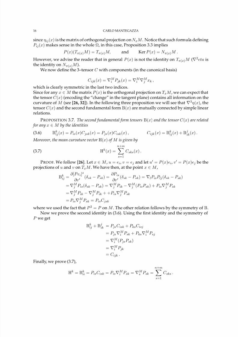
We now dene the 3–tensor C with components (in the canonical basis)

C ijk (x) = M i P jk (x) = M

iM j xk ,

which is clearly symmetric in the last two indices.Since for any x∈M the matrix P (x) is the orthogonal projection on T x M , we can expect thatthe tensor C (x) (encoding the “change” in the tangent plane) contains all information on thecurvature of M (see [26, 32]). In the following three proposition we will see that 3η(x), thetensor C (x) and the second fundamental form B(x) are mutually connected by simple linearrelations.

PROPOSITION 3.7. The second fundamental form tensorsB(x) and the tensor C (x) are related for anyx∈M by the identities

(3.6) Bkij (x) = P is (x)C jsk (x) = P js (x)C isk (x) , C ijk (x) = B k

ij (x) + B jik (x) .

Moreover, the mean curvature vectorH(x) of M is given by

(3.7) Hk (x) =n + m

s=1C sks (x) .

PROOF. We follow [ 26]. Let x∈M , u = ei , v = e j and let u = P (x)ei , v = P (x)e j be theprojections of u and v on T x M . We have then, at the point x∈M ,

Bkij =∂ [P e i ]s

∂v (δsk −P sk ) =∂P is∂v (δsk −P sk ) = lP is P lj (δsk −P sk )

= M j P is (δsk −P sk ) = M

j P ik − M j (P is P sk ) + P is M

j P sk

= M j P ik − M

j P ik + + P is M j P sk

= P is M j P sk = P is C jsk

where we used the fact that P 2 = P on M . The other relation follows by the symmetry of B.Now we prove the second identity in (3.6). Using the rst identity and the symmetry of

P we get

Bkij + B j

ik = P js C isk + P ks C isj

= P js M

iP sk + P ks

M

iP sj

= M i (P js P sk )

= M i P jk

= C ijk .

Finally, we prove (3.7),

Hk = B kii = P is C isk = P is M

i P sk = M s P sk =

n + m

s=1C sks .




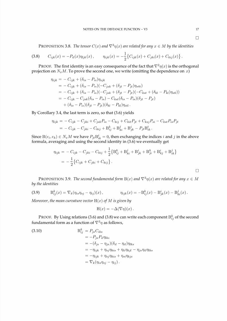
PROPOSITION 3.8. The tensor C (x) and 3η(x) are related for anyx∈M by the identities

(3.8) C ijk (x) = −P il (x)ηljk (x) , ηijk (x) = −12 C ijk (x) + C jki (x) + C kij (x) .

PROOF. The rst identity is an easy consequence of the fact that 2η(x) is the orthogonalprojection on N x M . To prove the second one, we write (omitting the dependence on x)

ηijk = −C ijk + ( δis −P is )ηsjk

= −C ijk + ( δis −P is )(−C jsk + ( δ jt −P jt )ηstk )= −C ijk + ( δis −P is )(−C jsk + ( δ jt −P jt )(−C kst + ( δkl −P kl )ηstl ))= −C ijk −C jsk (δis −P is ) −C kst (δis −P is )(δ jt −P jt )

+ ( δis −P is )(δ jt −P jt )(δkl −P kl )ηstl .

By Corollary 3.4, the last term is zero, so that (3.6) yieldsηijk = −C ijk −C jki + C jsk P is −C kij + C kit P jt + C ksj P si −C kst P is P jt

= −C ijk −C jki −C kij + B kij + B j

ki + B i jk −P jt Bt

ik .

Since B(ei , ek )∈N x M we have P jt Btik = 0 , then exchanging the indices i and j in the above

formula, averaging and using the second identity in (3.6) we eventually get

ηijk = −C ijk −C jki −C kij +12

Bkij + B j

ki + B i jk + B k

ji + B ikj + B j

ik

= −12

C ijk + C jki + C kij .

PROPOSITION 3.9. The second fundamental formB(x) and 3η(x) are related for anyx∈M by the identities

(3.9) Bkij (x) = k(ηis ηsj −ηij )(x) , ηijk (x) = −Bk

ij (x) −Bi jk (x) −B j

ki (x) .

Moreover, the mean curvature vectorH(x) of M is given by

H(x) = −∆( η)(x) .

PROOF. By Using relations (3.6) and (3.8) we can write each component Bkij of the second

fundamental form as a function of 3η

as follows,Bk

ij = P js C iks(3.10)= −P js P il ηlks

= −(δ js −η js )(δil −ηil )ηlks

= −ηijk + ηsj ηkis + ηli ηkjl −η js ηil ηlks

= −ηijk + ηsj ηkis + ηsi ηkjs

= k (ηis ηsj −ηij ) .



18 CARLO MANTEGAZZA

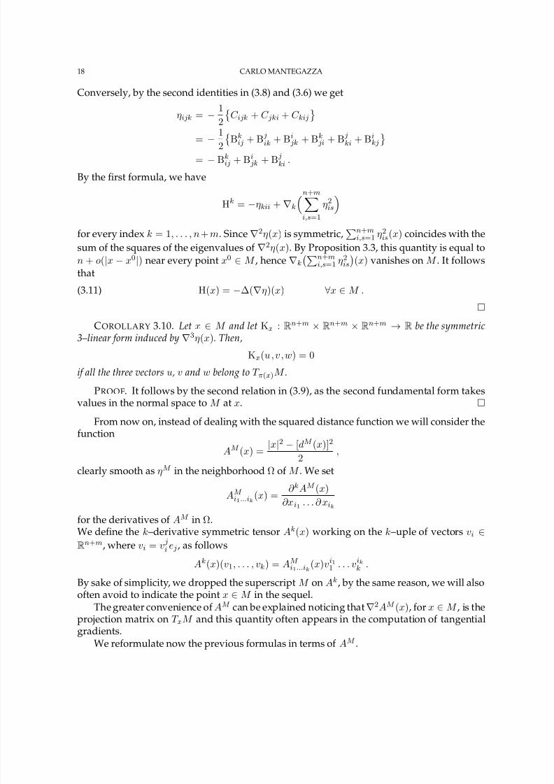
Conversely, by the second identities in (3.8) and (3.6) we get

ηijk = −12

C ijk + C jki + C kij

= −12 Bkij + B jik + B i jk + B k ji + B jki + B ikj

= −Bkij + B i

jk + B jki .

By the rst formula, we have

Hk = −ηkii + k

n + m

i,s =1

η2is

for every index k = 1 , . . . , n + m . Since 2η(x) is symmetric, n + mi,s =1 η2

is (x) coincides with thesum of the squares of the eigenvalues of 2η(x). By Proposition 3.3, this quantity is equal ton + o(|x −x0|) near every point x0

∈M , hence kn + mi,s =1 η2

is (x) vanishes on M . It follows

that(3.11) H(x) = −∆( η)(x) ∀x∈M .

COROLLARY 3.10. Let x ∈M and let Kx : R n + m ×R n + m ×R n+ m →R be the symmetric3–linear form induced by 3η(x). Then,

Kx (u,v,w ) = 0

if all the three vectorsu, v and w belong toT π (x)M .

PROOF. It follows by the second relation in (3.9), as the second fundamental form takesvalues in the normal space to M at x.

From now on, instead of dealing with the squared distance function we will consider thefunction

AM (x) = |x|2 −[dM (x)]2

2,

clearly smooth as ηM in the neighborhood Ω of M . We set

AM i1 ...i k (x) =

∂ kAM (x)∂x i1 . . . ∂ x ik

for the derivatives of AM in Ω.We dene the k–derivative symmetric tensor Ak(x) working on the k–uple of vectors vi ∈R n + m

, where vi = v ji e j , as follows

Ak (x)(v1, . . . , vk ) = AM i1 ...i k

(x)vi11 . . . v ik

k .

By sake of simplicity, we dropped the superscript M on Ak , by the same reason, we will alsooften avoid to indicate the point x∈M in the sequel.

The greater convenience of AM can be explained noticing that 2AM (x), for x∈M , is theprojection matrix on T x M and this quantity often appears in the computation of tangentialgradients.

We reformulate now the previous formulas in terms of AM .




PROPOSITION 3.11. The following properties of AM hold,

(a) for any x∈Ω, the vector AM (x) coincide with the projection pointπM (x) of x on M . Moreover, 2AM (x) is zero onN π (x)M and maps T π (x)M onto T π (x)M .If x∈M , then 2AM (x) is the matrix P of orthogonal projection onT x M ;

(b) for any x∈Ω, the 3–linear formKx : R k ×R k ×R k →R given by

Kx (u,v,w ) =n+ m

i,j,k =1

AM ijk (x)u i v j wk

is equal to zero if at least two of the 3 vectorsu , v, w, are normal toM at π(x) = AM (x)or if x∈M and the three vectors are all tangent;

(c) for x ∈M , the second fundamental formB(x) and the mean curvature vector H(x) are

related to the derivatives of AM

(x) by

(3.12) Bkij (x) = AM

js (x)AM il (x)AM

slk (x) = δkl −AM kl (x) AM

ijl (x),

(3.13) Hk (x) =n + m

j =1

AM jkj (x),

(3.14) M i AM

jk (x) = B kij (x) + B j

ik (x).

PROOF. The rst statement follows by Proposition 3.3 and the second one by Corol-lary 3.4. The rst equality in (3.12) and (3.13) follow by relations (3.11) and (3.10). The sec-ond equality in (3.12) can be obtained multiplying both sides of the second relation in (3.9) by the normal projection (I − 2AM ). Finally (3.14) is a restatement of the second equalityin (3.6).

By means of the relations in Propositions 3.7, 3.8, 3.9 we have the following estimates.

COROLLARY 3.12. At every point of M we have,

|C |2 ≤ | 3AM |2 = 3 |B|2 ≤3|C |2 .

PROOF. We have only to show the identity | 3AM |2 = 3 |B|2, the other inequalities areimmediate as the projection P is a 1–Lipschitz map.We compute in a orthonormal basis eisuch that e1, . . . , e n = T x M , by means of thesecond relation in (3.9), and keeping in mind that the second fundamental form B takes



20 CARLO MANTEGAZZA

values in the normal space N x M ,

| 3AM |2 =n

i,j,k =1

|ηijk |2

=n +1 ≤ i ≤ n + m

1 ≤ j,k ≤ n

|ηijk |2 +n +1 ≤ j ≤ n + m

1 ≤ i,k ≤ n

|ηijk |2 +n +1 ≤ k ≤ n + m

1 ≤ i,j ≤ n

|ηijk |2

=n +1 ≤ i ≤ n + m

1 ≤ j,k ≤ n

|Bkij + B i

jk + B jki |2 +

n +1 ≤ j ≤ n + m1 ≤ i,k ≤ n

|Bkij + B i

jk + B jki |2

+n +1 ≤ k ≤ n + m

1 ≤ i,j ≤ n

|Bkij + B i

jk + B jki |2

=n +1 ≤ i ≤ n + m

1 ≤ j,k ≤ n

|Bi jk |2 +

n +1 ≤ j ≤ n + m1 ≤ i,k ≤ n

|B jki |2 +

n +1 ≤ k ≤ n + m1 ≤ i,j ≤ n

|Bkij |2

= 3n +1 ≤ i ≤ n + m

1 ≤ j,k ≤ n

|Bi jk |2

= 3 |B|2 .

4. Higher Order Relations

In this section we work out some properties, about the higher derivatives of the squareof the distance function from a submanifold, in particular the relations with the covariant

derivatives of the second fundamental form. The main result here is a recurrence formulafor Ak (Proposition 4.1), that is, the tensor of k–derivatives of the squared distance functionfrom M , once its action is split on tangent and normal vectors. Such formula is crucial to get“structure information” and estimates on the tensors Ak (Corollary 4.3 and Proposition 4.6).

PROPOSITION 4.1. For everyk ≥2 and for everys∈ 0, . . . kthere exists a familypk,s j 1 ...j k − s

of symmetric polynomial tensors of type(s, 0) on M , where j 1, . . . , j k− s∈ 1, . . . , n + m, which arecontractions of the second fundamental formB and its covariant derivatives with the metric tensorg,such that

Ak(X 1, . . . , X s , N 1, . . . , N k− s ) = pk,s j 1 ...j k − s

(X 1, . . . , X s )N j 11 . . . N jk − s

k− s

for everys –uple of tangent vectorsX h and (k

−s) –uple of normal vectorsN h in R n + m (with the

obvious interpretation if s = 0 or s = k, that is, for instance in this latter case the symbols indexedby 1, . . . , k −s are not present in the formulas). Moreover, the tensorspk,s

j 1 ...j k − sare invariant by exchange of thej –indices and the maximum order

of differentiation of B which appears in everypk,s j 1 ...j k − s

is at most k −3, when k ≥ 3. Consideringthe tangent plane at any point x∈M also as a subset of R n + m , the polynomial tensorspk,s

j 1 ...j k − sare

expressed in the coordinate basis of the Euclidean space as follows

pk,s j 1 ...j k − s

(X 1, . . . , X s )N j 11 . . . N jk − s

k− s = pk,s j 1 ...j k − s ,i 1 ...i s

X i11 . . . X i s

s N j 11 . . . N jk − s

k− s .




Then, a family of tensors satisfying the above properties can be dened recursively according to the following formulas

p2,0 j 1 j 2

= p2,1 j 1 ,i 1

= 0 , p2,2i1 i2

= δi1 i2(4.1)

pk,0 j 1 ...j k

= pk,1 j 1 ...j k − 1 ,i 1

= 0 for everyk ≥2(4.2)

pk+1 ,s j 1 ...j k − s +1 ,i 0 i1 ...i s − 1

= ( pk,s − 1 j 1 ...j k − s +1

)i0 i1 ...i s − 1 if 2 ≤s < k + 1(4.3)

−k− s+1

h=1

pk,s − 1 j 1 ...j h − 1 rj h +1 ...j k − s +1 ,i 1 ...i s − 1

B jhri 0

−s− 1

h=1

pk,s − 2rj 1 ...j k − s +1 ,i 1 ...i h − 1 ih +1 ...i s − 1

Bri0 ih

+k− s+1

h=1

pk,s j 1 ...j h − 1 jh +1 ...j k − s +1 ,i 1 ...i s − 1 r B jh

ri 0

pk+1 ,k+1i0 i1 ...i k +1

= pk,ki0 i1 ...i k −

k

h=1

pk,k − 1r,i 1 ...i h − 1 ih +1 ...i k

Bri0 ih

.(4.4)

PROOF. If k = 2 we have immediately

A2(N 1, N 2) = 0 , A2(X 1, N 1) = 0 , A2(X 1, X 2) = X i1X i2 = δi1 i2 X i11 X i2

2

since X 1 and X 2 are tangent and A2 is the projection on the tangent space. Hence, for-mula (4.1) follows.We argue now by induction on k ≥2. When s = 0 the value Ak (N 1, . . . , N k )(x) depends onlyon the function AM on the m–dimensional normal subspace to M at x, and on this subspaceAM is identically zero, hence the rst equality in (4.2) is proved.Suppose now that s∈ 1, . . . , k + 1 , we extend the vectors X h ∈T x M and N h ∈N x M to afamily of local vector elds, respectively tangent and normal to M , then

Ak+1 (X 0, X 1, . . . , X s− 1, N 1, . . . , N k− s+1 ) =∂

∂X 0Ak (X 1, . . . , X s− 1, N 1, . . . , N k− s+1 )

−s− 1

h=1

Ak X 1, . . . X h− 1,∂X h∂X 0

, X h+1 , . . . , X s− 1, N 1, . . . , N k− s+1

−k− s+1

h=1

Ak X 1, . . . , X s− 1, N 1, . . . ,∂N h∂X 0

, . . . , N k− s+1

where the last line is not present in the special case s = k + 1 and the second line is notpresent if s = 1 . In this last case, we have

Ak+1 (X 0, N 1, . . . , N k) =∂

∂X 0Ak (N 1, . . . , N k ) −

k

h=1

Ak N 1, . . . ,∂N h∂X 0

, . . . , N k = 0

since the rst term of the right member is zero by the rst equality in (4.2) and, after decom-posing ∂N h

∂X 0in tangent and normal part, the tangent term is zero by induction and the normal



22 CARLO MANTEGAZZA

term is zero for (4.2) again. This shows the second equality in (4.2).So we suppose 1 < s < k + 1 , by the inductive hypothesis,

Ak(X 1, . . . , X s− 1, N 1, . . . , N k− s+1 ) = p

k,s − 1 j 1 ...j k − s +1 (X 1, . . . , X s− 1)N

j 1

1 . . . N jk − s +1

k− s+1

thus, differentiating along X 0, which is a tangent eld, we obtain

Ak+1 (X 0,X 1, . . . , X s− 1, N 1, . . . , N k− s+1 )

=∂

∂X 0 pk,s − 1

j 1 ...j k − s +1(X 1, . . . , X s− 1)N j 1

1 . . . N jk − s +1

k− s+1

−s− 1

h=1

Ak X 1, . . . ,∂X h∂X 0

M , . . . , X s− 1, N 1, . . . , N k− s+1

−s− 1

h=1

Ak X 1, . . . , ∂X h∂X 0

⊥

, . . . , X s− 1, N 1, . . . , N k− s+1

−k− s+1

h=1

Ak X 1, . . . , X s− 1, N 1, . . . ,∂N h∂X 0

M , . . . , N k− s+1

−k− s+1

h=1

Ak X 1, . . . , X s− 1, N 1, . . . ,∂N h∂X 0

⊥

, . . . , N k− s+1 .

We use now the symmetry of Ak and we substitute recursively pk,s , pk,s − 1 and pk,s − 2 to Ak ,

according to the number of tangent vectors inside Ak

,

Ak+1 (X 0,X 1, . . . , X s− 1, N 1, . . . , N k− s+1 )

=∂

∂X 0 pk,s − 1

j 1 ...j k − s +1(X 1, . . . , X s− 1) N j 1

1 . . . N jk − s +1

k− s+1

+k− s+1

h=1

pk,s − 1 j 1 ...j k − s +1

(X 1, . . . , X s− 1)N j 11 . . .

∂N jhh

∂X 0. . . N jk − s +1

k− s+1

−s− 1

h=1

pk,s − 1 j 1 ...j k − s +1

(X 1, . . . , X 0 X h , . . . , X s− 1)N j 11 . . . N jk − s +1

k− s+1

−s− 1

h=1

pk,s − 2rj 1 ...j k − s +1

(X 1, . . . , X h− 1, X h+1 , . . . , X s− 1)∂X h∂X 0

⊥ rN j 1

1 . . . N jk − s +1

k− s+1

−k− s+1

h=1

pk,s j 1 ...j h − 1 jh +1 ...j k − s +1

X 1, . . . , X s− 1,∂N h∂X 0

M N j 1

1 . . . N jh − 1

h− 1 N jh +1

h+1 . . . N jk − s +1

k− s+1

−k− s+1

h=1

pk,s − 1 j 1 ...j k − s +1

(X 1, . . . , X s− 1)N j 11 . . .

∂N h∂X 0

⊥ jh. . . N jk − s +1

k− s+1 .




Adding the rst and the third line on the right hand side we get the covariant derivative of the tensor pk,s − 1

j 1 ...j k − s +1times N j 1

1 . . . N jk − s +1

k− s+1 , adding the second and the last line we get

Ak+1 (X 0,X 1, . . . , X s− 1, N 1, . . . , N k− s+1 )

= pk,s − 1 j 1 ...j k − s +1

(X 0, X 1, . . . , X s− 1)N j 11 . . . N jk − s +1

k− s+1

+k− s+1

h=1

pk,s − 1 j 1 ...j k − s +1

(X 1, . . . , X s− 1)N j 11 . . .

∂N h∂X 0

M jh. . . N jk − s +1

k− s+1

−s− 1

h=1

pk,s − 2rj 1 ...j k − s +1

(X 1, . . . , X h− 1, X h+1 , . . . , X s− 1)∂X h∂X 0

⊥ rN j 1

1 . . . N jk − s +1

k− s+1

−

k− s+1

h=1

pk,s j 1 ...j h − 1 jh +1 ...j k − s +1

X 1, . . . , X s− 1,∂N h

∂X 0

M N j 1

1 . . . N jh − 1

h− 1 N jh +1

h+1 . . . N jk − s +1

k− s+1 .

Taking now into account that

∂N h∂X 0

M r=

∂N h∂X 0

,∂

∂x i

∂ ∂x i

r= − N h ,

∂ ∂X 0

∂ ∂x i

∂ ∂x i

, er = −B jhri 0

X i00 N jh

h ,

where ∂ ∂x i i=1 ,...,n

is a basis of the tangent space of M , and

∂X h∂X 0

⊥ r= B r

i0 ihX i0

0 X ihh ,

substituting, we get

Ak+1 (X 0,X 1, . . . , X s− 1, N 1, . . . , N k− s+1 )

= pk,s − 1 j 1 ...j k − s +1

(X 0, X 1, . . . , X s− 1)N j 11 . . . N jk − s +1

k− s+1

−k− s+1

h=1

pk,s − 1 j 1 ...j h − 1 rj h +1 ...j k − s +1

(X 1, . . . , X s− 1)B jhri 0

X i00 N j 1

1 . . . N jk − s +1

k− s+1

−s− 1

h=1

pk,s − 2rj 1 ...j k − s +1

(X 1, . . . , X h− 1, X h+1 , . . . , X s− 1)B ri0 ih

X i00 X ih

h N j 11 . . . N jk − s +1

k− s+1

+k− s+1

h=1

pk,s j 1 ...j h − 1 jh +1 ...j k − s +1

(X 1, . . . , X s− 1, B jhri 0

X i00 er )N j 1

1 . . . N jk − s +1

k− s+1 .



24 CARLO MANTEGAZZA

Then, expressing the tensors in coordinates, we have

Ak+1 (X 0,X 1, . . . , X s− 1, N 1, . . . , N k− s+1 )

= ( pk,s − 1 j 1 ...j

k − s+1

) i0 i1 ...i s − 1 X i00 X i1

1 . . . X i s − 1

s− 1 N j 11 . . . N jk − s +1

k− s+1

−k− s+1

h=1

pk,s − 1 j 1 ...j h − 1 rj h +1 ...j k − s +1 ,i 1 ...i s − 1

B jhri 0

X i00 . . . X i s − 1

s− 1 N j 11 . . . N jk − s +1

k− s+1

−s− 1

h=1

pk,s − 2rj 1 ...j k − s +1 ,i 1 ...i h − 1 ih +1 ...i s − 1

Bri0 ih

X i00 . . . X i s − 1

s− 1 N j 11 . . . N jk − s +1

k− s+1

+k− s+1

h=1

pk,s j 1 ...j h − 1 jh +1 ...j k − s +1 ,i 1 ...i s − 1 r B jh

ri 0X i0

0 . . . X i s − 1

s− 1 N j 11 . . . N jk − s +1

k− s+1 ,

which is formula (4.3).In the special case s = k + 1 , to get formula (4.4), we just have to repeat the computationsdropping all the lines containing sums like k− s+1

h=1 ... , which are not present.Finally, assuming inductively that the polynomial tensors pk,s , pk,s − 1 and pk,s − 2 are symmet-ric in the j –indices and contain covariant derivatives of B only up to the order k −3 (whenk ≥3), also the claims about the symmetry and the order of the derivatives of B follow.

EXAMPLE 4.2. We compute some pk,s as a consequence of this proposition.(1) When k = 2 we saw that

p2,0 j 1 j 2

= 0 , p2,1 j 1

= 0 , p2,2 = g .

(2) When k = 3 we have, by means of formulas (4.2) and (4.3),

p3,0 j 1 j2 j 3 = 0 , p3,1 j 1 j 2 = 0

p3,2 j 1 ,i 1 i2

= p2,2i2 r B j 1

ri 1= B j 1

i1 i2

p3,3i1 i2 i3

= ( p2,2)i1 i2 i3 + p2,1r,i 2

Bri1 i3 + p2,1

r,i 3Br

i1 i2 = 0

that is, p3,2

j 1= B j 1 and p3,3 = 0 .

(3) When k = 4 we have,

p4,0 j 1 j 2 j 3 j 4

= 0 , p4,1 j 1 j 2 j 3

= 0

p4,2 j 1 j 2 ,i 1 i2

= p3,2 j 1 ,i 1 r B j 2

ri 2+ p3,2

j 2 ,i 1 r B j 1ri 1

= B j 1i1 r B j 2

ri 2+ B j 2

i2 r B j 1ri 1

p4,3 j 1 ,i 1 i2 i3 = ( p3,2 j 1 )i1 i2 i3 + p3,2r,i 2 i3 B j 1ri 1 = ( p3,2 j 1 )i1 i2 i3 + B ri2 i3 B j 1ri 1 = ( B j 1 )i1 i2 i3

since we contracted a normal vector with a tangent one,

p4,4i1 i2 i3 i4

= − p3,2r i3i4Br

i1 i2 − p3,2r i2i4Br

i1 i3 − p3,2r i2i3Br

i1 i4

= −Bri3 i4 Br

i1 i2 −Bri2 i4 Br

i1 i3 −Bri2 i3 Br

i1 i4 .

Proposition 4.1 allows us to write Ak in terms of the tensors pk,s and the projections onthe tangent and normal spaces (hence contracting with the scalar product of R n + m ), so weget the following corollary.




COROLLARY 4.3. For every k ≥ 3 the symmetric tensor Ak can be expressed as a polynomialtensor in B and its covariant derivatives, contracted with the scalar product of R n + m .The maximum order of differentiation of B which appears in Ak is k −3. More precisely, the onlytensors among thepk,s containing such highest derivative arepk,k − 1

j 1, given by

pk,k − 1 j 1

= k− 3B j 1 + LOT .

where we denoted withLOT (lower order terms ) a polynomial term containing only derivatives of B up to the order k-4.

PROOF. Looking at the tensors with the derivative of B of maximum order among the pk,s

j 1 ...j k − s, by formula (4.3) and the fact that the only non zero polynomials p3,s

j 1 ...j 3 − s ,i 1 ...i s are p3,2

j 1 ,i 1 i2= B j 1

i1 i2 (see Example 4.2), it is clear that they come from the derivative pk− 1,k − 2 j 1 .

Iterating the argument, the leading term in pk,k − 1 j1

is given by k− 3 p3,2 j 1

= k− 3B j 1 .

REMARK 4.4. We can see in Example 4.2 that when k = 3 and 4, the lower order term

which appears above is zero. Actually, by a tedious computation, one can see that for k ≥5this is no more true.

COROLLARY 4.5. For everyk ≥3 we have the following estimates at every pointx∈M ,

C 1| k− 3B|2 + LOT 1 ≤ |Ak|2 ≤C 2| k− 3B|2 + LOT 2

where the two constantsC 1 and C 2 depends only onk, n and m , and LOT 1 and LOT 2 are polynomialterms containing only derivatives of B up to the order k-4. Moreover, for a couple of “universal” functionsF 1 and F 2 depending only onk, n and m , we have

k

i=3|Ai |2 ≤F 1

k− 3

i=0| iB|2

k− 3

i=0| i B|2 ≤F 2

k

i=3|Ai|2 .

PROOF. The rst estimates follow by Corollary 4.3 and the structure of Ak obtained inProposition 4.1. The second statement is obtained by such estimates, by iteration.

The decomposition of Ak in its tangent and normal components is very useful in study-ing in even more detail the norm of Ak .

Fixing at a point x∈M an orthonormal basis e1, . . . , e n + mof R n + m such that e1, . . . , e nis a basis of T x M , we have obviously

|Ak|2 =1≤ i1 ,...,i k ≤ n + m

[Ak (ei1 , . . . , e ik )]2

≥1 ≤ i 1 ,i 2 ≤ n

n<i 3 ,...,i k ≤ n + m

[Ak (ei1 , ei2 , ei3 , . . . , e ik )]2

≥n<j ≤ n + m 1≤ i1 ,i 2 ≤ n

[Ak (ei1 , ei2 , e j , . . . , e j )]2

=n<j ≤ n + m 1≤ i1 ,i 2 ≤ n

[ pk,2 j...j,i 1 i2

]2 ,



26 CARLO MANTEGAZZA

that is,

|Ak|2 ≥n<j ≤ n + m

| pk,2 j...j |2 .

We analyse this last term by means of formula (4.3). We have p2,2

= g and for every k ≥2,

pk+1 ,2 j...j,i 0 i1

=k− 1

h=1

pk,2 j...j,i 1 r B j

ri 0= ( k −1) pk,2

j...j,i 1 r B jri 0

.

Then, by induction, it is easy to see that

pk,2 j...j,i 0 i1

= ( k −2)!B ji0 r 1

B jr 1 r 2 . . . B j

r k − 3 i1

hence, as the bilinear form B j is symmetric, denoting with λ js its eigenvalues at the point

x∈M , we conclude

| pk,2

j...j

|2 = [( k

−2)!]2

n

s=1(λ j

s )2(k− 2)

≥C

|B j

|2k− 4 .

Coming back to our estimate,

|Ak|2 ≥C n<j ≤ n + m

|B j |2k− 4 ≥C n<j ≤ n + m

|B j |2k− 2

= C |B|2k− 4 .

PROPOSITION 4.6. The following estimate holds,

|Ak|2 ≥C |B|2k− 4

where C is a universal constant depending only onk, n and m .

5. The Distance Function on Riemannian Manifolds

In this section we discuss more in detail some analytic properties of the distance functionthat we state without proof in Section 3.We consider in full generality the distance function dK from a closed set K of a Riemann-ian manifold (M, g ) and we analyse the connection with the theory of viscosity solutions of Hamilton–Jacobi equations. Indeed, we will see that the distance function is a viscosity so-lution of the following Hamilton–Jacobi problem

| u| = 1 in M \ K ,u = 0 on ∂K

and we will use the property of semiconcavityshared by such solutions to analyse the prop-

erties of dK

(for more details see [ 33]).5.1. Stationary Hamilton–Jacobi Equations on Manifolds. Let M be a smooth and con-

nected, n–dimensional, differentiable manifold.We consider the following Hamilton–Jacobi problem in Ω⊂M ,

H(x,du (x), u(x)) = 0 in Ω,u = u0 on ∂ Ω

where H : T ∗Ω ×R →R and T ∗denotes the cotangent bundle.




DEFINITION 5.1. Given a continuous function u : Ω →R and a point x∈M , the superdifferential of u at x is the subset of T ∗x M dened by

∂ + u(x) = dϕ(x)

|ϕ

∈

C 1(M ),ϕ(x)

−u(x) = min

M

ϕ

−u .

Similarly, the set

∂ − u(x) = dψ(x) |ψ∈C 1(M ), ψ(x) −u(x) = maxM

ψ −u

is called the subdifferentialof u at x.Notice that it is equivalent to replace the max (min) on all M with the maximum (minimum)in an open neighborhood of x in M .

It is easy to see that ∂ + u(x) and ∂ − u(x) are both nonempty if and only if u is differen-tiable at x∈M . In this case we have

∂ + u(x) = ∂ − u(x) =

du(x)

.

We list here without proof some of the standard properties of the sub and superdifferentialswhich will be needed later.

PROPOSITION 5.2. If ψ : N →M is a map between the smooth manifoldsN and M which isC 1 around x∈N , then

∂ + (u ψ)(x)⊃∂ + u(ψ(x)) dψ(x) = v dψ(x) |v∈∂ + u(ψ(x)).

If ψ is a local diffeomorphism nearx, the inclusion becomes an equality. An analogous statementholds for∂ − .

PROPOSITION 5.3. If θ : R →R is a C 1 function such that θ (u(x)) ≥0, then∂ + (θ u)(x)⊃dθ(u(x)) ∂ + u(x) = dθ(u(x)) v |v∈∂ + u(x),

similarly for ∂ − . If θ (u(x)) > 0 then the inclusion is an equality.For a locally Lipschitz function u on a Riemannian manifold (M, g), ∂ + u(x) and ∂ − u(x)

are compact convex sets, almost everywhere coinciding with the differential of the functionu, by Rademacher’s theorem.For a generic continuous function u we prove in the next proposition that ∂ + u(x) and ∂ − u(x)are not empty in a dense subset.

PROPOSITION 5.4. Let u : Ω →R be a continuous function on an open subsetΩ of M . Thenthe subdifferential∂ − u(x) (the superdifferential ∂ + u(x)) is not empty for everyx in a dense subsetof Ω.

PROOF. It is always possible to endow M with a Riemannian structure giving a metric

d(·, ·) on M which generates the same topology.Consider a generic point y ∈Ω and a geodesic ball B contained in Ω with center y. If the ball B is small enough, the function x →d2(x, y) is smooth in B . Taking a large positiveconstant A, the function F A(x) = u(x) + Ad2(x, y) has a local minimum at a point xA in theinterior of B . At xA the subdifferential of the function F A must contain the origin of T ∗xA M ,hence, being d2(x, y) differentiable in the ball B , the differential of −d2(x, y) at xA belongs to∂ − u(xA). As the point y and the ball B were arbitrarily chosen, the set of points where thesubdifferential of u is not empty is dense in Ω.The same argument holds for the superdifferential of u , considering the function −u.



28 CARLO MANTEGAZZA

Now we introduce the notion of semiconcavity which will play a central role.

DEFINITION 5.5. Given an open set Ω⊂R n , a continuous function u : Ω →R is called

locally semiconcaveif, for any open convex set Ω ⊂Ω with compact closure in Ω, there exists

a constant C such that one of the following three equivalent conditions is satised,(1) ∀x, h with x , x + h , x −h∈Ω ,

u(x + h) + u(x −h) −2u(x) ≤2C |h|2 ,

(2) u(x) −C |x|2 is a concave function in Ω ,(3) D 2u ≤2C Id in Ω , as distributions ( Id is the n ×n identity matrix).

In order to give a meaning to the concept of semiconcavity when the ambient space is adifferentiable manifold M , we analyse the stability of this property under composition withC 2 maps.

PROPOSITION 5.6. Let Ω and Ω two open subsets of R n . If u : Ω →R is a Lipschitz functionsuch that u(x)

−C

|x

|2 is concave andψ : Ω

→Ω is a C 2 function with bounded rst and second

derivatives, then u ψ : Ω →R is a Lipschitz function and u ψ(y) −C |y|2 is concave, for asuitable constant C .

The proof is straightforward. Then, the following denition is well–posed.

DEFINITION 5.7. A continuous function u : M →R is called locally semiconcaveif, for anylocal chart ψ : R n →Ω⊂M , the function u ψ is locally semiconcave in R n .

The importance of semiconcave functions in connection with the generalized differen-tials is expressed by the following proposition (see [ 10]).

PROPOSITION 5.8. Let the functionu : M →R be locally semiconcave, then the superdifferen-tial ∂ + u is not empty at each point, moreover,∂ + v is upper semicontinuous , namely

xk →x, vk →v, vk∈∂

+u(xk ) =⇒ v∈∂

+u(x) .

In particular, if the differentialdu exists at every point of Ω∈M , then u∈C 1(Ω).

Now we introduce the denition of viscosity solution.Let Ω be an open subset of M and H, called Hamiltonian function, a continuous real functionon T ∗Ω ×R . We are interested in the following Hamilton–Jacobi problem(5.1) H(x,du (x), u(x)) = 0 in Ω.

DEFINITION 5.9. We say that a continuous function u is a viscosity solution of equa-tion (5.1) if for every x∈Ω,

(5.2)H(x,v,u (x)) ≤0 ∀v∈∂ + u(x) ,

H(x,v,u (x)) ≥0 ∀v∈∂ −

u(x) .If only the rst condition is satised (respectively, the second) u is called a viscosity subsolu-tion (respectively, a viscosity supersolution).

If Ω is an open subset of another smooth differentiable manifold N and ψ : Ω →Ωis a C 1 local diffeomorphism, we dene the pull–back of the Hamiltonian function ψ∗H :T ∗Ω ×R →R by

ψ∗H(y,v,r ) = H( ψ(y), v dψ(y)− 1, r ) .Taking into account Proposition 5.2, the following statement is obvious.




PROPOSITION 5.10. If u is a viscosity solution of H = 0 in Ω⊂M and ψ : Ω →Ω is a C 1local diffeomorphism, thenu ψ is a viscosity solution of ψ∗H = 0 in Ω ⊂N .

5.2. The Distance Function from a Closed Subset of a Manifold. From now on, (M, g)

will be a smooth, connected and complete, Riemannian manifold without boundary, of di-mension n .

We consider a closed and not empty subset K and the distance function dK : M →R

from K , which is dened as the inmum of the lengths of the C 1 curves starting at x andending at K . As M is complete, by the Theorem of Hopf–Rinow, such inmum is reached by at least one curve which will be a smooth geodesic. We will also consider the functionηK = [dK ]2/ 2 as in the previous sections.

In the following we will denote the distance between two points x, y ∈M with d(x, y)and the exponential map of (M, g ) with Exp : T M ×R →M . For simplicity, we will write |v|for the modulus of a vector v∈T M , dened as g(v, v).

PROPOSITION 5.11. The distance functiondK is the unique viscosity solution of the following Hamilton–Jacobi problem

(5.3) | u|2 −1 = 0 in M \ K ,u = 0 on K

in the class of continuous functions bounded from below.The function ηK is the unique viscosity solution of

(5.4) | u|2 −2u = 0 in M ,u = 0 on K

in the class of continuous functions onM such that their zero set isK .REMARK 5.12. The restriction to lower bounded functions is necessary, x and − x

are both viscosity solutions of Problem (5.3) with M = R n and K = 0. Moreover, thecompleteness of M plays an important role here, if M is the open unit ball of R n the sameexample shows that the uniqueness does not hold.Notice also that every function [dH ]2/ 2 where H is a closed subset of M with H ⊃K , is aviscosity solution of Problem (5.4), equal to zero on K .

PROOF. The quantity dK (x) is the minimum time t ≥ 0 for any curve γ to reach a pointγ (t)∈K , subject to the conditions γ (0) = 0 and |γ | ≤1; the function dK is then the valuefunction of a “minimum time problem”; this proves that dK is also a viscosity solution of

Problem (5.3), by well known results (see for example [ 5, Chap. 4, Prop. 2.3]). Then we showthat the function ηK is a solution of Problem (5.4).First of all, notice that the distance function from K is a 1–Lipschitz function, hence ηK islocally Lipschitz.As dK is 1–Lipschitz, at every point of K the function ηK is differentiable and its differentialis zero. Hence, the denition of viscosity solution holds also for points belonging to K .In order to prove the thesis, it is then sufcient to test conditions (5.2) on the generalizeddifferentials at the points of the open set M \ K .Since ηK is positive in M \ K , applying Proposition 5.3 with the function θ(t) = √2t , we see



30 CARLO MANTEGAZZA

that the function ηK is a viscosity solution of

gu

√2u,

u√2u −1 = 0

in M \ K . Being there positive, it also solvesg( u, u) −2u = 0

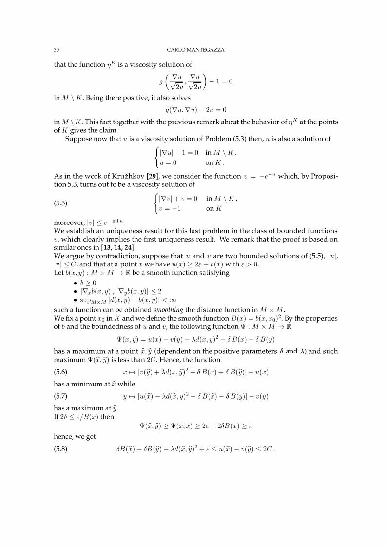
in M \ K . This fact together with the previous remark about the behavior of ηK at the pointsof K gives the claim.

Suppose now that u is a viscosity solution of Problem (5.3) then, u is also a solution of

| u| −1 = 0 in M \ K ,u = 0 on K .

As in the work of Kru zhkov [ 29], we consider the function v = −e− u which, by Proposi-tion 5.3, turns out to be a viscosity solution of

(5.5) | v|+ v = 0 in M \ K ,v = −1 on K

moreover, |v| ≤e− inf u .We establish an uniqueness result for this last problem in the class of bounded functionsv, which clearly implies the rst uniqueness result. We remark that the proof is based onsimilar ones in [ 13, 14, 24].We argue by contradiction, suppose that u and v are two bounded solutions of (5.5), |u|,|v| ≤C , and that at a point x we have u(x) ≥2ε + v(x) with ε > 0.Let b(x, y ) : M ×M →R be a smooth function satisfying

•b

≥0

• | x b(x, y)|, | yb(x, y)| ≤2

• sup M × M |d(x, y) −b(x, y)| < ∞such a function can be obtained smoothing the distance function in M ×M .We x a point x0 in K and we dene the smooth function B (x) = b(x, x 0)2. By the propertiesof b and the boundedness of u and v, the following function Ψ : M ×M →R

Ψ(x, y) = u(x) −v(y) −λd(x, y)2 −δ B(x) −δ B(y)

has a maximum at a point x, y (dependent on the positive parameters δ and λ) and suchmaximum Ψ( x, y) is less than 2C . Hence, the function

(5.6) x →[v(

y) + λd(x,

y)2 + δ B(x) + δ B(

y)] −u(x)

has a minimum at x while(5.7) y →[u( x) −λd( x, y)2 −δ B( x) −δ B(y)] −v(y)

has a maximum at y.If 2δ ≤ε/B (x) then

Ψ( x, y) ≥Ψ(x, x ) ≥2ε −2δB (x) ≥εhence, we get

(5.8) δB ( x) + δB ( y) + λd( x, y)2 + ε ≤u( x) −v( y) ≤2C .




This shows that, for a xed δ, the pair x, y is contained in a bounded set and, if λ goes to + ∞the distance between x and y goes to zero. Possibly passing to a subsequence for λ going toinnity, x and y converge to a common limit point z which cannot belong to K , otherwisewe would get ε

≤u(z)

−v(z) = 0 , thus, for some λ large enough also x and y do not belong

to K .As the function d2(x, y) is smooth in Bz ×Bz ⊂M ×M , where Bz is a small geodesic ballaround z, choosing a suitable λ large enough we can differentiate the functions inside thesquare brackets in equations (5.6) and (5.7) obtaining

v = δ B ( x) + λ x d2( x, y) ∈∂ + u( x) ,

w = −δ B ( y) −λ yd2( x, y) ∈∂ − v( y) .By Denition 5.9 we have that | v|+ u( x) ≤0 and | w|+ v( y) ≥0, hence

u( x) −v( y) + | v| − | w| ≤0 .

Moreover,

| v| − | w| = δ B ( v) + λ x d2( x, y) − δ B ( y) + λ yd

2( x, y)

≥ λ x d2( x, y) − λ yd2( x, y) − |δ B ( y)| − |δ B ( x)|= 2 λd( x, y) | x d( x, y)| −2λd( x, y) | yd( x, y)| − |δ B ( y)| − |δ B ( x)|= 2 λd( x, y) −2λd( x, y) − |δ B ( y)| − |δ B ( x)|= − |δ B ( y)| − |δ B ( x)|

which implies,u( x) −v( y) −δ| B ( y)| −δ| B ( x)| ≤0 .

Finally, we have that

δ| B (

x)| = 2 δ|b(

x, x 0) b(

x, x 0)| ≤4δ

B (

x)

and using the estimate δB ( x) ≤2C which follows from equation (5.8),δ| B ( x)| ≤8√2δC ≤ε/ 4

if δ was chosen small enough. Holding the same for y, we conclude thatu( x) −v( y) −ε/ 2 ≤0

which is in contradiction with the fact that u( x) −v( y) ≥ε.About the second uniqueness claim, if u is a continuous viscosity solution of Prob-

lem (5.4) then, by Proposition 5.4 the superdifferential of u is not empty in a dense subset of M \ K , hence, directly by the equation and by continuity, u is non negative. By the hypothe-sis on its zero set we conclude that u is positive in all M \ K . Composing u with the functiont

→√2t , we see that √2u is a positive, continuous viscosity solution of Problem (5.3), then

it must coincide with dK , by the previous result. It follows that u = ηK .

We now study the singular set of dK ,

Sing = x∈M |ηK is not differentiable at x .

REMARK 5.13. In this denition we used the squared distance function instead of thedistance in order to avoid to consider also the points of the boundary of K , which are singu-lar for dK but not for ηK . It is trivial to see that outside K the distance and its square havethe same regularity.



32 CARLO MANTEGAZZA

PROPOSITION 5.14. The function dK is locally semiconcave inM \ K .

PROOF. The distance function dK is a viscosity solution of H = 0 in M \ K , where theHamiltonian function is given by H(x,v, t ) = |v|2 −1. We choose a smooth local chart ψ :

Rn

→Ω ⊂M and we dene v = dK

ψ, which is a locally Lipschitz function and, byProposition 5.10, it is a viscosity solution of ψ∗H = 0 .The pull–back of the Hamiltonian function on R n takes the form

ψ∗H(y,w,s ) = gψ(y)(dψ(w), dψ(w)) −1 = gij (y)wi w j −1

for (y,w,s )∈R n ×R n ×R and where gij (y) are the components of the metric tensor of M in

local coordinates.Since the matrix gij (y) is positive denite ψ∗H(y,w,s ) is locally uniformly convex in w,hence, by Theorem 5.3 of [ 30], it follows that v = dK ψ is locally semiconcave in R n . Recall-ing Denition 5.7, this means that dK is locally semiconcave in M \ K .

The semiconcavity of dK allows us to work with the superdifferentials when the gradi-

ent does not exist. Indeed, it follows that the points of Sing are precisely those where thesuperdifferential is not a singleton and the following result is a straightforward consequenceof Proposition 5.8.

PROPOSITION 5.15. The function ηK is of classC 1 in the open setM \ Sing and dK is C 1 inM \ K ∪Sing .

The semiconcavity property also gives information about the relations between the struc-ture of the superdifferential at a point x and the set of minimal geodesics from x to K (see [1, 2, 33]).The set Ext (∂ + ηK (x)) of extremal points of the (convex) superdifferential set of ηK at x isin one–to–one correspondence with the family G(x) of minimal geodesics from x to K . Pre-cisely

G(x) is described by

(5.9) G(x) = Exp( x, −v, ·) | [0, 1] →M |for v∈Ext (∂ + ηK (x)) .

Hence, the set of points of K at minimum distance from x are given by Exp( x, −v, 1) for vin the set of extremal points of the superdifferential set of ηK at x. As a particular case wehave that if the function ηK is differentiable at x if and only if the point of K closest to x isuniquely determined and given by Exp( x, − ηK (x), 1).

We consider now a set K which is a k–dimensional, embedded C r submanifold of M without boundary, with 0 ≤k ≤n −1 (the case k = n is trivial) and r ≥2.

For every p∈K we consider the following three subsets of T pM ,

• T pK , the vector subspace of tangent vectors to K at p,

• N pK = w∈T pM |g p(w, T pK ) = 0, the vector subspace of normal vectors to K at

p,• U pK = w∈N pK |g p(w, w) = 1, the subset of unit normal vectors to K at p,then the bundles NK = ( p,v) |v∈N pK and UK = ( p,v) |v∈U pK inherit the structureof T M . Being K a C r submanifold of M , the bundles NK and UK are respectively n–dimensional and (n −1)–dimensional C r − 1 submanifolds of T M .Notice that in the special case K = p, we have that NK = T pM and UK = S n − 1

⊂T pM .We dene the map F : UK ×R + →M as the restriction of the exponential map of M to

UK ,F ( p,v,t ) = Exp( p,v,t ) ∀( p,v)∈UK and t∈

R + .




Since UK is a C r − 1 manifold and the exponential map of M is smooth, F and all its deriva-tives with respect to the variable t are of class C r − 1.

REMARK 5.16. If a minimal geodesic, parametrized by arc length, starts at a point p∈M

and arrives at a point q∈K , its velocity vector v at q has to belong to U qK , otherwise thecondition of minimality is easily contradicted.Since the geodesics, parametrized by arc length, ending on K are given by the family of mapst →F (q ,v, t ) with (q, v)∈UK , the distance from K of a point p is given by the formula

(5.10) dK ( p) = inf t∈R + | (q,v, t )∈F − 1( p),

which obviously becomes dK ( p) = πR + F − 1( p) when the counterimage is a singleton (themap πR + is the projection on the second factor of the product UK ×R + ).The study of the singularities of the squared distance function then reduces to the analysisof the (possibly set valued) map F − 1.This problem, from the topological point of view, is naturally connected with the study of the singularities of continuous maps between Euclidean spaces. For instance, when K co-incides with a single point of M the singular sets were shown to be related to the classes of singularities considered by the Theory of Catastrophes, see [9].

Let us dene the C r − 1 map exp : NK →M byexp ( p,v) = Exp( p,v, 1) ∀( p,v)∈NK.

At the points ( p, 0)∈NK the map exp is differentiable and d exp ( p, 0) is invertible betweenT ( p,0) NK and T pM , indeed T ( p,0) NK can be identied with T pM and under such identica-tion d exp ( p, 0) is the identity. Since, by hypothesis, the map exp is at least C 1, it follows thatin a neighborhood of ( p, 0) in NK the differential of exp is invertible, hence the map exp isa C r − 1 local diffeomorphism. Holding the relation F ( p,v,t ) = exp ( p,vt), we conclude thatfor small t > 0, the map F is a local diffeomorphism.Being K at least C 2, by a standard result in differential geometry, there exists an open tubularneighborhoodΩ of K in M formed by non intersecting, minimal geodesics starting normallyfrom K . Hence, by the previous discussion and possibly choosing a smaller tubular neighborhood Ω of K , the map F − 1 is well dened and C r − 1 in Ω \ K (see for instance, [ 4]).Then, the gradient of ηK exists in Ω and we have, by relations (5.9) and (5.10),

ηK ( p) = dK ( p)∂F ∂t

(F − 1( p)) .

Since dK = πR + F − 1( p) ∈C r − 1 in Ω and the functions F , ∂F ∂t are of class C r − 1, it follows

that ηK is C r − 1 and ηK is C r in Ω\K . The same C r regularity in Ω\K follows immediatelyalso for the distance function dK .Moreover, the function ηK is C r regular also on the set K , hence in the whole neighborhoodΩ, as the square regularizes the jump of the gradient in the direction normal to K , see [3, 4].

We summarize these results in the following proposition which has as a particular caseProposition 3.1.

PROPOSITION 5.17. If K is a regular submanifold of classC r , with r ≥2, then there exists anopen subset Λ of UK ×R + with the property that if (q,v, t ) ∈Λ then also (q,v,s ) ∈Λ for every0 < s < t , and an open neighborhoodΩ of K in M , such that the map F |Λ : Λ →Ω \ K is adiffeomorphism. Moreover,



34 CARLO MANTEGAZZA

• for every point inΩ there is an unique point of minimum distance inK (unique projectionproperty in Ω),

• the distance function dK is C r in Ω \ K ,

•the squared distance functionηK is C r in Ω.

REMARK 5.18. It can be proved that C 1,1 is the minimal regularity of K to have theunique projection property in a neighborhood, in this case also the squared distance functionturns out to be of class C 1,1 (see [20, 22] and also [ 15, 16] for a detailed discussion of therelation between the regularity of K and of dK .

References1. G. Alberti, L. Ambrosio, and P. Cannarsa, On the singularities of convex functions, Manuscripta Math. 76 (1992),

421–435.2. L. Ambrosio, P. Cannarsa, and H. M. Soner, On the propagation of singularities of semi–convex functions, Ann.

Sc. Norm. Sup. Pisa 20 (4) (1993), 597–616.3. L. Ambrosio and C. Mantegazza, Curvature and distance function from a manifold, J. Geom. Anal. 8 (1998), no. 5,

723–748, Dedicated to the memory of Fred Almgren.4. L. Ambrosio and H. M. Soner, A level set approach to the evolution of surfaces of any codimension, J. Diff. Geom.

43 (1996), 693–737.5. M. Bardi and I. Capuzzo Dolcetta, Optimal control and viscosity solutions of Hamilton–Jacobi–Bellman equations,

Systems & Control: Foundations & Applications, Birkh auser BostonInc., Boston, MA, 1997, With appendices by Maurizio Falcone and Pierpaolo Soravia.

6. J. Berndt, S. Console, and C. Olmos, Submanifolds and holonomy, Chapman & Hall/CRC Research Notes inMathematics, vol. 434, Chapman & Hall/CRC, Boca Raton, FL, 2003.

7. P. O. Bonnet, M´ emoire sur la th´ eorie des surfaces applicables sur une surface donn´ ee, J. de l’Ecole Polytechnique,Paris 24 (1865), 209–230.

8. , M´ emoire sur la th´ eorie des surfaces applicables sur une surface donn´ ee, J. de l’Ecole Polytechnique, Paris25 (1867), 1–151.

9. M. Buchner, The structure of the cut–locus in dim≤ 6 , Compositio Math. 37 (1978), 103–119.

10. P. Cannarsa and H. M. Soner, On the singularities of the viscosity solutions to Hamilton–Jacobi–Bellman equations,Indiana Univ. Math. J. 36 (1987), 501–524.

11. Y. G. Chen, Y. Giga, and S. Goto, Uniqueness and existence of viscosity solutions of generalized mean curvature owequations, J. Diff. Geom. 33 (1991), 749–786.

12. D. Codazzi, Sulle coordinate curvilinee d’una supercie e dello spazio. i, ii, iii, 1867–1871.13. M. G. Crandall, L. C. Evans, and P.-L. Lions, Some properties of viscosity solutions of Hamilton–Jacobi equations,

Trans. Amer. Math. Soc. 282 (1984), 487–502.14. M. G. Crandall, H. Ishii, and P.-L. Lions, User’s guide to viscosity solutions of second order partial differential

equations, Bull. Amer. Math. Soc. 27/1 (1992), 1–67.15. M. Delfour and J.-P. Zol´esio, Shape analysis via oriented distance functions, J. Funct. Anal. 123 (1994), 129–201.16. , Shape analysis via distance functions: local theory, Boundaries, interfaces and transitions (M. Delfour,

ed.), CRM Proc. Lect. Notes Ser., AMS, 1998.17. M. P. Do Carmo, Riemannian geometry, Birkhauser, Boston, 1992.18. L. C. Evans and J. Spruck, Motion of level sets by mean curvature I , J. Diff. Geom. 33 (1991), 635–681.19. , Motion of level sets by mean curvature II , Trans. Amer. Math. Soc. 330 (1992), no. 1, 321–332.20. H. Federer, Curvature measures, Trans. Amer. Math. Soc. 93 (1959), 418–491.21. , Geometric measure theory, Springer–Verlag, 1969.22. J. H. G. Fu,Tubular neighbourhoods in euclidean spaces, Duke Math. J. 52 (1985), 1025–1046.23. S. Gallot, D. Hulin, and J. Lafontaine, Riemannian geometry, Springer–Verlag, 1990.24. Y. Giga, S. Goto, H. Ishii, and M. H. Sato, Comparison principle and convexity preserving properties for singular

degenerate parabolic equations on unbounded domains, Indiana Univ. Math. J. 40 (1991), no. 2, 443–469.25. D. Gilbarg and N. S. Trudinger, Elliptic partial differential equations of second order, Springer–Verlag, 1983.26. J. E. Hutchinson, Second fundamental form for varifolds and the existence of surfaces minimizing curvature, Indiana

Univ. Math. J. 35 (1986), 45–71.




27. S. Kobayashi and K. Nomizu, Foundations of differential geometry. Vol. I , Wiley Classics Library, John Wiley &Sons Inc., New York, 1996.

28. , Foundations of differential geometry. Vol. II , Wiley Classics Library, John Wiley & Sons Inc., New York,1996.

29. S. N. Kruzhkov, generalized solutions of the Hamilton–Jacobi equations of eikonal type, I. Math. USSR Sb. 27 (1975),406–446.30. P.-L. Lions, Generalized solutions of Hamilton–Jacobi equations, Pitman, Boston, 1982.31. G. Mainardi, Su la teoria generale delle superci, Giornale dell’I. R. Lombardo di Scienze, Lettere ed Arti 9

(1856), 385–399.32. C. Mantegazza, Curvature varifolds with boundary, J. Diff. Geom. 43 (1996), 807–843.33. C. Mantegazza and A. C. Mennucci, Hamilton–Jacobi equations and distance functions on Riemannian manifolds,

Appl. Math. Opt. 47 (2003), no. 1, 1–25.34. S. Osher and J. Sethian, Fronts propagating with curvature–dependent speed: algorithms based on Hamilton–Jacobi

formulations, J. Comput. Phys. 79 (1988), no. 1, 12–49.35. K. M. Peterson, ¨ Uber die Biegung der Fl¨ achen, Ph.D. thesis, Doctoral Thesis, Dorpat Univ., 1853.36. L. Simon, Lectures on geometric measure theory, Proc. Center Math. Anal., vol. 3, Australian National Univer-

sity, Canberra, 1983.37. J. Simons, Minimal varieties in Riemannian manifolds, Ann. of Math. (2) 88 (1968), 62–105.

(Carlo Mantegazza) S CUOLA N ORMALE SUPERIORE P ISA, ITALY, 56126E-mail address, C. Mantegazza: [email protected]

Distance Notes

Documents

Transcript of Distance Notes