Distance Metric Learning: Beyond 0/1...

Distance Metric Learning: Beyond 0/1 Loss

Praveen Krishnan

CVIT, IIIT Hyderabad

June 14, 2017

1

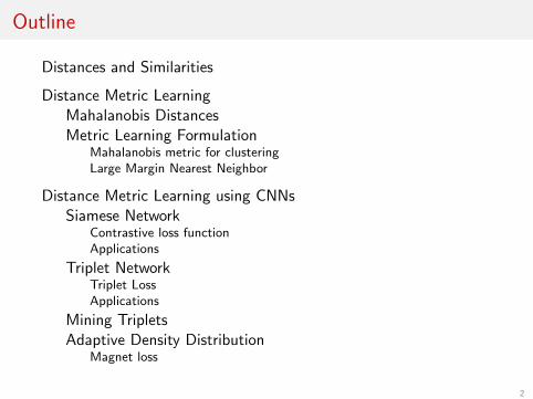
Outline

Distances and Similarities

Distance Metric LearningMahalanobis DistancesMetric Learning Formulation

Mahalanobis metric for clusteringLarge Margin Nearest Neighbor

Distance Metric Learning using CNNsSiamese Network

Contrastive loss functionApplications

Triplet NetworkTriplet LossApplications

Mining TripletsAdaptive Density Distribution

Magnet loss

2


Distance FunctionsThe concept of distance function d(., .) is inherent to any patternrecognition problem. E.g. clustering (kmeans), classification (kNN,SVM) etc.

Typical Choices

I Minkowski Distance: Lp(P,Q) = (∑

i |Pi − Qi |p)1p .

I Cosine: L(P,Q) = PTQ|P||Q|

I Earth Mover: Uses an optimization algorithm

I Edit distance: Uses dynamic programming between sequences.

I KL Divergence: KL(P ‖ Q) =∑

i Pi log PiQi

. (Not Symmetric!)

I many more ... (depending on type of problem)

3


Choosing the right distance function?

Image Credit: Brian Kulis, ECCV’10 Tutorial on Distance Functions and Metric Learning.

4

Metric Learning

Distance Metric Learning

Learn a function that maps input patterns into a target space suchthat the simple distance in the target space (Euclidean)approximates the “semantic” distance in the input space.

Figure 1: Hadsell et. al. CVPR’06

5

Metric Learning

Many applications

Figure 2: A subset of applications using metric learning.

I Scale to large number of #categories. [Schroff et al., 2015]

I Fine grained classification . [Rippel et. al., 2015]

I Visualization of high-dimensional data. [van der Maaten andHinton, 2008]

I Ranking and retrieval. [Wang et. al. CVPR’14]

6

Properties of a Metric

What defines a metric?

1. Non-negativity: D(P,Q) ≥ 0

2. Identity of indiscernibles: D(P,Q) = 0 iff P = Q

3. Symmetry: D(P,Q) = D(Q,P)

4. Triangle Inequality: D(P,Q) ≤ D(P,K ) + D(K ,Q)

Pseudo/Semi Metric

If the second property is not followed strictly i.e. “iff→ if”

7

Metric learning as learning transformations

I Feature WeightingI Learn weightings over the features, then use standard distance

(e.g.,Euclidean) after re-weighting

I Full linear transformationI In addition to scaling of features, also rotates the dataI For transformations to r < d dimensions, this is linear

dimensionality reduction

I Non Linear TransformationI Neural netsI Kernelization of linear transformations

Slide Credit: Brian Kulis, ECCV’10 Tutorial on Distance Functions and Metric Learning.

8

Supervised Metric Learning

Main focus of this talk.

I Constraints or labels given to the algorithm. E.g. set ofsimilarity and dissimilarity constraints

I Recent popular methods uses CNN architecture for non-lineartransformation.

Before getting into deep architectures, let us explore some basicand classical works.

9

Mahalanobis Distances

I Assume the data is represented as N vectors of length d:X = [x1, x2, · · · , xN ]

I Squared Euclidean distance

d(x1, x2) = ||x1 − x2||22= (x1 − x2)T (x1 − x2)

(1)

I Let Σ =∑

i ,j(xi − µ)(xj − µ)T

I The original Mahalanobis distance is given as:-

dM(x1, x2) = (x1 − x2)TΣ−1(x1 − x2) (2)

10


Equivalent to applying a whitening transform

Image Credit: Brian Kulis, ECCV’10 Tutorial on Distance Functions and Metric Learning.

11


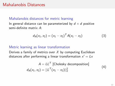
Mahalanobis distances for metric learning

In general distance can be parameterized by d × d positivesemi-definite matrix A:

dA(x1, x2) = (x1 − x2)TA(x1 − x2) (3)

Metric learning as linear transformation

Derives a family of metrics over X by computing Euclideandistances after performing a linear transformation x ′ = Lx

A = LLT [Cholesky decomposition]

dA(x1, x2) = ||LT (x1 − x2)||22(4)

12


Why is A positive semi-definite (PSD)?

I If A is not PSD, then dA could be negative.

I Suppose v = x1 − x2 is an eigen vector corresponding to anegative eigenvalue λ of A

dA(x1, x2) = (x1 − x2)TA(x1 − x2)

= vTAv

= λvT v < 0

(5)

13

Metric Learning Formulation

Two main components:-

I A set of constraints on the distanceI A regularizer on the distance / objective function

Constrained Case

minA r(A)

s.t. ci (A) ≤ 0 0 ≤ i ≤ C

A ≥ 0

(6)

Here r is the regularizer. Popular one is ||A||2F .A ≥ 0 for positive semi-definiteness.

Unconstrained Case

minA≥0

r(A) + λC∑i=1

ci (A) (7)

14

Metric Learning Formulation: Defining Constraints

Similarity / Dissimilarity constraints

Given a set of pairs (xi , xj) S of points that should be similar, anda set of pairs of points D of points that should be dissimilar.

dA(xi , xj) ≤ l ∀(i , j) ∈ S

dA(xi , xj) ≥ u ∀(i , j) ∈ D(8)

Popular in verification problems.

Relative distance constraintsGiven a triplet (xi , xj , xk) such that the distance between xi and xjshould be smaller than the distance between xi and xk :-

dA(xi , xj) ≤ dA(xi , xk)−m (9)

Here m is the margin. It is popular for ranking problems.

15

Mahalanobis metric for clustering

Key Components

I A convex objective function for distance metric learning.

I Similar to linear discriminant analysis.

maxA∑

(xi ,xj )∈D

√dA(xi , xj)

s.t. c(A) =∑

(xi ,xj )∈S

dA(xi , xj) ≤ 1

A ≥ 0

(10)

I Here, D is a set of pairs of dissimilar pairs, S is a set ofsimilar pairs

I Objective tries to maximize sum of dissimilar distances

I Constraint keeps sum of similar distances small

Xing et. al.’s NIPS’0216

Large Margin Nearest Neighbor

Key Components

Learns a Mahalanobis distance metric using:-

I convex loss function

I margin maximizationI constraints imposed for accurate kNN classification.

I Promotes local distance notion instead of global similarity.

Intuition

I Each training input xi should share the same label yi as its knearest neighbors and,

I Training inputs with different labels should be widelyseparated.

Weinberger et. al. JMLR’0917


Target Neighbors

Use prior knowledge or compute k nearest neighbors using Euclideandistance. Neighbors does not change while training.

Imposters

Differently labeled inputs that invade the perimeter plus unit margin.

||LT (xi − xl)||2 ≤ ||LT (xi − xj)||2 + 1 (11)

Here xi and xj have label yi and xl is an imposter with label yl 6= yiWeinberger et. al. JMLR’09 18


Loss Function

εpull(L) =∑j i

||LT (xi − xj)||2

εpush(L) =∑i ,j i

∑l

(1− yil)[1 + ||LT (xi − xj)||2 − ||LT (xi − xl)||2]+

(12)Here [z ]+ = max(0, z), denotes the standard hinge loss.

ε(L) = (1− µ)εpull(L) + µεpush(L). (13)

Here (xi , xj , xl) forms a triplet sample. The above loss function isnon-convex and the original paper discuss a convex formulationusing semi-definite programming.

Weinberger et. al. JMLR’0919

Distance Metric Learning using CNNs

Siamese NetworkSiamese is an informal term for conjoined or fused.

I Contains two or more identical sub-networks with shared setof parameters and weights

I Popularly used for similarity learning tasks such as verificationand ranking.

Figure 3: Signature verification. Bromley et. al. NIPS’93

20

Siamese Architecture

Given a family of functions GW (X ) parameterized by W , find Wsuch that the similarity metric DW (X1,X2) is small for similar pairsand large for disimilar pairs:-

DW (X1,X2) = ||GW (X1)− GW (X2)|| (14)

Chopra et. al. CVPR’05 and Hadsell et. al. CVPR’0621

Contrastive Loss Function

Let X1,X2 ∈ I, pair of input vectors and Y be the binary labelwhere Y = 0 means the pair is similar and Y = 1 means dissimilar.We define a parameterized distance function DW as:-

DW (X1,X2) = ||GW (X1)− GW (X2)||2 (15)

The contrastive loss function is given as:-

L(W ,Y ,X1,X2) = (1− Y )1

2(DW )2 + (Y )

1

2{max(0,m − DW )}2

(16)Here m > 0 is the margin which enforces the robustness.

22

Contrastive loss function

Spring model analogy: F = −KX

Attraction

∂LS∂W

= DW∂DW

∂W

Repulsion

∂LD∂W

= −(m − DW )∂DW

∂W

The force is absent whenDW ≥ m.

23

Dimensionality Reduction

24

Face Verification

Discriminative Deep Metric Learning

I Face verification inthe wild.

I Defines a thresholdfor both positive andnegative face pairs.

Hu et. al. CVPR’1425

Face Verification

Discriminative Deep Metric Learning

arg minf

1

2

∑i ,j

g(1− lij(τ − d2f (xi , xj))) +

λ

2

M∑m=1

(||Wm||2F + ||bm||22)

Here g(z) = 1β log(1 + exp(βz)) is generalized logistic regression

function.

Hu et. al. CVPR’1426

Triplet network

From the idea of triplet pairs as formulated in LMNN, the siamesearchitecture is modified to a triplet network:-

Figure 4: Triplet Network

27

Triplet Loss

I Learn an embedding function f (.) that assigns smallerdistances to similar image pairs.

I Given a triplet: ti = (pi , p+i , p

−i ), triplet loss is defined as:-

l(pi , p+i , p

−i ) = max{0,m+D(f (pi ), f (p+i+))−D(f (pi ), f (p−i ))}

Figure 5: Network architecture of deep ranking model

Wang et. al. CVPR’1428

Fine-grained Image Similarity with Deep Ranking


FaceNet

Face Embedding

I State of the art results on LFW dataset.

I Additional constrain of embedding to live on thed-dimensional hypersphere, ||f (x)||2 = 1.

I Use an online triplet selection method.

Figure 6: Results of Face Clustering using learned embedded features.

Schroff et. al. arxiv’1530

How to mine triplets?

Selection of triplets important for faster convergence and bettertraining.

Challenges

I Given N examples, picking all triplets is O(N3).

I Need for fresh selection of triplets after each epoch.

Typical Strategies

I Select hard positives and hard negatives.

I Generate triplets offline every n steps ‘or’ online from eachmini batch.

31

How to mine triplets?

Schroff et. al. arxiv’15

I Generate triplets online with large mini batch sizes by ensuringminimum no. of exemplars for each class.

I Picks semi-hard examples where:-

||G (X ai )− G (X p

i )||22 < ||G (X ai )− G (X n

i )||22

These negative samples are further away from anchor but lieinside the margin m


I Uses pairwise relevance scores (prior knowledge).

I Uses an online triplet sampling algorithm based on reservoirsampling.

32

Issues in the Existing Approaches

I Predefined target neighborhood structureI Defined a-priori using supervised knowledge.I Doesn’t enable utilizing shared structure among different

classes.I Local similarity given by LMNN [Weinberger et. al. 2009],

partly attempts this issue however,I Target neighbors are determined a-priori and never updated

again.

I Objective formulationI Penalizing individual pairs of triplets does not employ sufficient

contextual insights of neighborhood structure.

I Non optimal mining of triplets leads to slower convergenceand non-optimal solutions.

33

Issues in the Existing Approaches

Figure 7: Both triplet and softmax result in unimodal separation, due toenforcement of semantic similarity.

Image Credit: Rippel et. al. arxiv’1634

Magnet Loss

Key Points

I Adaptive assessment of similarity as function of currentrepresentation.

I Local discrimination by penalizing class distribution overlap.

I Enabling clustering based approach for efficient hard negativemining.

Rippel et. al. arxiv’1635

Magnet Loss

Model FormulationJointly manipulate clusters in pursuit of local discrimination.For each class c , we have K cluster assignments given as:-

Ic1 . . . IcK = arg minIc1 ...IcK

K∑k=1

∑r∈I ck

||r − µck ||22,

µck =1

|I ck |∑r∈I ck

r

Here rn = f (xn,Θ), denote the representation given by a CNNnetwork.


Magnet Loss

Model FormulationThe magnet loss is defined as:-

L(Θ) =1

N

N∑n=1

{− logexp

12σ2 ||rn−µ(rn)||22−α∑

c 6=C(rn)

∑Kk=1 exp

12σ2 ||rn−µ(rn)||22

}

Here C (r) is the class of representation r and µ(r) is the assignedcluster center. α ∈ R and σ2 = 1

N−1∑

r∈D ||r − µ(r)||22 is thevariance.

Key points

I Loss for examples farther from cluster centers minimum.

I Variance standardization for in-variance against characteristiclength scale.

I α acts as the cluster separation gap.


Magnet Loss

Training Procedure

I Neighbourhood samplingI Sample a seed cluster I1 ∼ pI(.)I Retrieve M − 1 nearest impostor clusters of I2, . . . IM of I1I For each cluster IM ,m = 1 . . .M, sample D examples

xm1 , . . . , xmD ∼ pIM

(.)Here pI ∝ LI and pIM

is a uniform distribution.

I Cluster Index: Periodic computation of Kmeans clusteringusing the current representation taken from the CNN network.

Figure 8: Triplet vs.magnet in terms of training curves.


References

Jane Bromley, Isabelle Guyon, Yann LeCun, Eduard Sackinger,Roopak Shah, ”Signature Verification Using a Siamese TimeDelay Neural Network”. NIPS 1993

Chopra, Sumit and Hadsell, Raia and LeCun, Yann, ”Learninga similarity metric discriminatively, with application to faceverification”, CVPR2005

Hadsell, Raia and Chopra, Sumit and LeCun, Yann,”Dimensionality reduction by learning an invariant mapping”,CVPR06

Brian Kulis, Distance Functions and Metric Learning: Part 2ECCV 2010 Tutorial

Weinberger, Kilian Q., and Lawrence K. Saul. ”Distancemetric learning for large margin nearest neighborclassification.” JMLR 2009.

39

Hu, Junlin, Jiwen Lu, and Yap-Peng Tan. ”Discriminative deepmetric learning for face verification in the wild.” CVPR 2014.

Wang, Jiang, et al. ”Learning fine-grained image similaritywith deep ranking.” CVPR 2014.

Schroff, Florian, Dmitry Kalenichenko, and James Philbin.”Facenet: A unified embedding for face recognition andclustering.” arXiv preprint (2015).

Rippel, Oren, et al. ”Metric learning with adaptive densitydiscrimination.” arXiv 2015.

40

Thank You

41

Distance Metric Learning: Beyond 0/1...

Documents

Transcript of Distance Metric Learning: Beyond 0/1...