Distance Dependent Chinese Restaurant Processes

Journal of Machine Learning Research 12 (2011) 2461-2488 Submitted 10/09; Revised 12/10; Published 8/10

Distance Dependent Chinese Restaurant Processes

David M. Blei [email protected]

Department of Computer SciencePrinceton UniversityPrinceton, NJ 08544, USA

Peter I. Frazier [email protected]

School of Operations Research and Information EngineeringCornell UniversityIthaca, NY 14853, USA

Editor: Carl Edward Rasmussen

Abstract

We develop the distance dependent Chinese restaurant process, a flexible class of distributions overpartitions that allows for dependencies between the elements. This class can be used to model manykinds of dependencies between data in infinite clustering models, including dependencies arisingfrom time, space, and network connectivity. We examine the properties of the distance depen-dent CRP, discuss its connections to Bayesian nonparametric mixture models, and derive a Gibbssampler for both fully observed and latent mixture settings. We study its empirical performancewith three text corpora. We show that relaxing the assumption of exchangeability with distancedependent CRPs can provide a better fit to sequential data andnetwork data. We also show thatthe distance dependent CRP representation of the traditional CRP mixture leads to a faster-mixingGibbs sampling algorithm than the one based on the original formulation.

Keywords: Chinese restaurant processes, Bayesian nonparametrics

1. Introduction

Dirichlet process (DP) mixture models provide a valuable suite of flexible clustering algorithms forhigh dimensional data analysis. Such models have been adapted to text modeling (Teh et al., 2006;Goldwater et al., 2006), computer vision (Sudderth et al., 2005), sequential models (Dunson, 2006;Fox et al., 2007), and computational biology (Xing et al., 2007). Moreover, recent years have seensignificant advances in scalable approximate posterior inference methodsfor this class of models(Liang et al., 2007; Daume, 2007; Blei and Jordan, 2005). DP mixtures have become a valuable toolin modern machine learning.

DP mixtures can be described via the Chinese restaurant process (CRP), a distribution overpartitions that embodies the assumed prior distribution over cluster structures(Pitman, 2002). TheCRP is fancifully described by a sequence of customers sitting down at the tables of a Chineserestaurant. Each customer sits at a previously occupied table with probabilityproportional to thenumber of customers already sitting there, and at a new table with probability proportional to aconcentration parameter. In a CRP mixture, customers are identified with data points, and datasitting at the same table belong to the same cluster. Since the number of occupied tables is random,this provides a flexible model in which the number of clusters is determined by thedata.

c©2011 David M. Blei and Peter I. Frazier.

BLEI AND FRAZIER

The customers of a CRP are exchangeable—under any permutation of theirordering, the prob-ability of a particular configuration is the same—and this property is essential toconnect the CRPmixture to the DP mixture. The reason is as follows. The Dirichlet process is a distribution overdistributions, and the DP mixture assumes that the random parameters governing the observationsare drawn from a distribution drawn from a Dirichlet process. The observations are conditionallyindependent given the random distribution, and thus they must be marginallyexchangeable.1 If theCRP mixture did not yield an exchangeable distribution, it could not be equivalent to a DP mixture.

Exchangeability is a reasonable assumption in some clustering applications, but in many it is not.Consider data ordered in time, such as a time-stamped collection of news articles. In this setting,each article should tend to cluster with other articles that are nearby in time. Or,consider spatial data,such as pixels in an image or measurements at geographic locations. Here again, each datum shouldtend to cluster with other data that are nearby in space. While the traditional CRPmixture providesa flexible prior over partitions of the data, it cannot accommodate such non-exchangeability.

In this paper, we develop thedistance dependent Chinese restaurant process, a new CRP inwhich the random seating assignment of the customers depends on the distances between them.2

These distances can be based on time, space, or other characteristics. Distance dependent CRPscan recover a number of existing dependent distributions (Ahmed and Xing, 2008; Zhu et al., 2005).They can also be arranged to recover the traditional CRP distribution. Thedistance dependentCRP expands the palette of infinite clustering models, allowing for many usefulnon-exchangeabledistributions as priors on partitions.3

The key to the distance dependent CRP is that it represents the partition withcustomer assign-ments, rather than table assignments. While the traditional CRP connects customers totables, thedistance dependent CRP connects customers to other customers. The partition of the data, thatis, the table assignment representation, arises from these customer connections. When used in aBayesian model, the customer assignment representation allows for a straightforward Gibbs sam-pling algorithm for approximate posterior inference (see Section 3). This provides a new tool forflexible clustering of non-exchangeable data, such as time-series or spatial data, as well as a newalgorithm for inference with traditional CRP mixtures.

1.1 Related Work

Several other non-exchangeable priors on partitions have appearedin recent research literature.Some can be formulated as distance dependent CRPs, while others represent a different class ofmodels. The most similar to the distance dependent CRP is the probability distribution on partitionspresented in Dahl (2008). Like the distance dependent CRP, this distribution may be constructedthrough a collection of independent priors on customer assignments to othercustomers, which thenimplies a prior on partitions. Unlike the distance dependent CRP, however, the distribution pre-

1. That these parameters will exhibit a clustering structure is due to the discreteness of distributions drawn from aDirichlet process (Ferguson, 1973; Antoniak, 1974; Blackwell, 1973).

2. This is an expanded version of our shorter conference paper on this subject (Blei and Frazier, 2010). This versioncontains new perspectives on inference and new results.

3. We avoid calling these clustering models “Bayesian nonparametric” (BNP) because they cannot necessarily be cast asa mixture model originating from a random measure, such as the DP mixture model. The DP mixture is BNP becauseit includes a prior over the infinite space of probability densities, and the CRPmixture is only BNP in its connectionto the DP mixture. That said, most applications of this machinery are basedaround letting the data determine theirnumber of clusters. The fact that it actually places a distribution on the infinite-dimensional space of probabilitymeasures is usually not exploited.

2462

DISTANCE DEPENDENTCHINESE RESTAURANT PROCESSES

sented in Dahl (2008) requires normalization of these customer assignmentprobabilities. The modelin Dahl (2008) may always be written as a distance dependent CRP, although the normalization re-quirement prevents the reverse from being true (see Section 2). We notethat Dahl (2008) does notpresent an algorithm for sampling from the posterior, but the Gibbs samplerpresented here for thedistance dependent CRP can also be employed for posterior inference inthat model.

There are a number of Bayesian nonparametric models that allow for dependence between(marginal) partition membership probabilities. These include the dependent Dirichlet process(MacEachern, 1999) and other similar processes (Duan et al., 2007; Griffin and Steel, 2006; Xueet al., 2007). Such models place a prior on collections of sampling distributionsdrawn from Dirich-let processes, with one sampling distribution drawn per possible value of covariate and samplingdistributions from similar covariates more likely to be similar. Marginalizing out the sampling dis-tributions, these models induce a prior on partitions by considering two customers to be clustered to-gether if their sampled values are equal. (Recall, these sampled values are drawn from the samplingdistributions corresponding to their respective covariates.) This prior need not be exchangeable ifwe do not condition on the covariate values.

Distance dependent CRPs represent an alternative strategy for modeling non-exchangeability.The difference hinges on marginal invariance, the property that a missingobservation does not af-fect the joint distribution. In general, dependent DPs exhibit marginal invariance while distancedependent CRPs do not. For the practitioner, this property is a modeling choice, which we discussin Section 2. Section 4 shows that distance dependent CRPs and dependent DPs represent nearlydistinct classes of models, intersecting only in the original DP or CRP.

Still other prior distributions on partitions include those presented in Ahmed andXing (2008)and Zhu et al. (2005), both of which are special cases of the distance dependent CRP. Rasmussenand Ghahramani (2002) use a gating network similar to the distance dependent CRP to partitiondatapoints among experts in way that is more likely to assign nearby points to the same cluster. Alsoincluded are the product partition models of Hartigan (1990), their recentextension to dependenceon covariates (Muller et al., 2008), and the dependent Pitman-Yor process (Sudderth and Jordan,2008). A review of prior probability distributions on partitions is presented inMueller and Quintana(2008). The Indian Buffet Process, a Bayesian non-parametric prior on sparse binary matrices, hasalso been generalized to model non-exchangeable data by Miller et al. (2008). We further discussthese priors in relation to the distance dependent CRP in Section 2.

The rest of this paper is organized as follows. In Section 2 we develop thedistance dependentCRP and discuss its properties. We show how the distance dependent CRPmay be used to modeldiscrete data, both fully-observed and as part of a mixture model. In Section 3 we show how thecustomer assignment representation allows for an efficient Gibbs sampling algorithm. In Section 4we show that distance dependent CRPs and dependent DPs represent distinct classes of models. Fi-nally, in Section 5 we describe an empirical study of three text corpora using the distance dependentCRP. We show that relaxing the assumption of exchangeability with distance dependent CRPs canprovide a better fit to sequential data. We also show its alternative formulationof the traditional CRPleads to a faster-mixing Gibbs sampling algorithm than the one based on the original formulation.

2463

BLEI AND FRAZIER

Figure 1: An illustration of the distance dependent CRP. The process operates at the level of cus-tomer assignments, where each customer chooses either another customer or no customeraccording to Equation (2). Customers that chose not to connect to another are indicatedwith a self link The table assignments, a representation of the partition that is familiar tothe CRP, are derived from the customer assignments.

2. Distance-dependent CRPs

The Chinese restaurant process (CRP) is a probability distribution over partitions (Pitman, 2002). Itis described by considering a Chinese restaurant with an infinite number oftables and a sequentialprocess by which customers enter the restaurant and each sit down at arandomly chosen table.After N customers have sat down, their configuration at the tables represents a random partition.Customers sitting at the same table are in the same cycle.

In the traditional CRP, the probability of a customer sitting at a table is computed from thenumber of other customers already sitting at that table. Letzi denote the table assignment of theith customer, assume that the customersz1:(i−1) occupyK tables, and letnk denote the number ofcustomers sitting at tablek. The traditional CRP draws eachzi sequentially,

p(zi = k|z1:(i−1),α) ∝{

nk for k≤ Kα for k= K+1,

(1)

whereα is a given scaling parameter. When allN customers have been seated, their table assign-ments provide a random partition. Though the process is described sequentially, the CRP is ex-changeable. The probability of a particular partition ofN customers is invariant to the order inwhich they sat down.

We now introduce thedistance dependent CRP. In this distribution, the seating plan probabilityis described in terms of the probability of a customer sitting with each of the othercustomers.The allocation of customers to tables is a by-product of this representation.If two customers are

2464


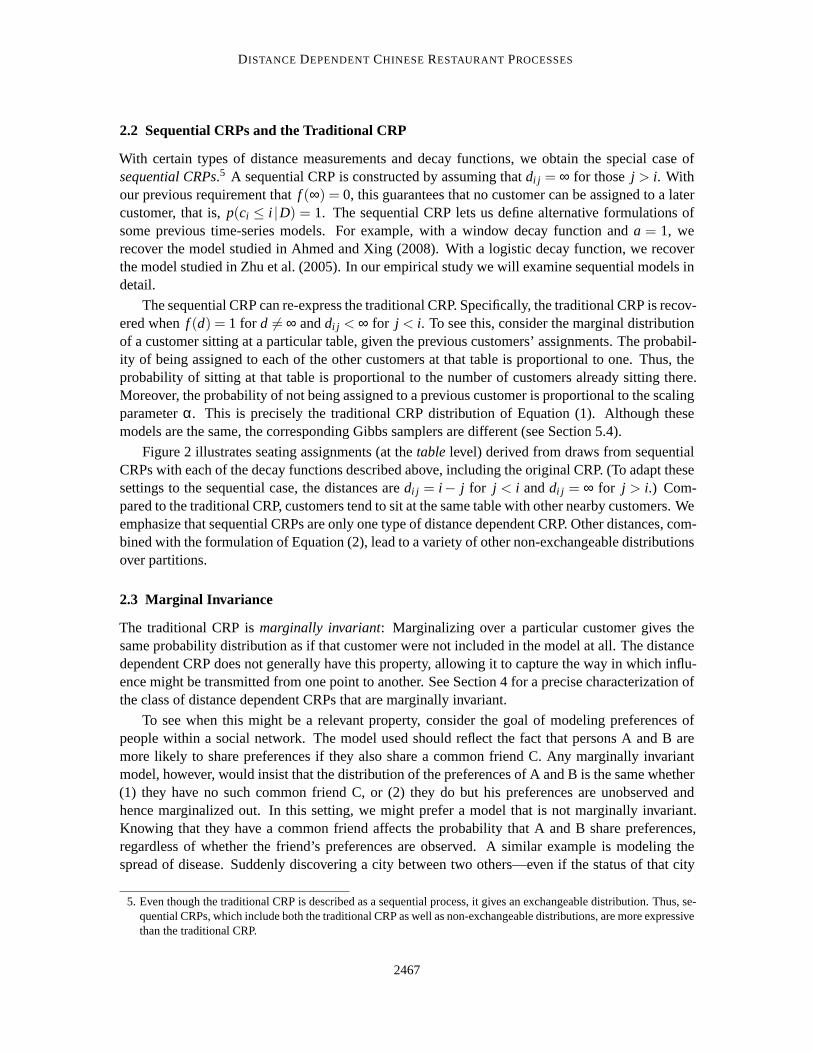
Figure 2: Draws from sequential CRPs. Illustrated are draws for different decay functions, whichare inset: (1) The traditional CRP; (2) The window decay function; (3) The exponentialdecay function; (4) The logistic decay function. The table assignments areillustrated,which are derived from the customer assignments drawn from the distancedependentCRP. The decay functions (inset) are functions of the distance between the current cus-tomer and each previous customer.

2465

BLEI AND FRAZIER

reachable by a sequence of interim customer assignments, then they at the same table. This isillustrated in Figure 1.

Let ci denote theith customer assignment, the index of the customer with whom theith customeris sitting. Letdi j denote the distance measurement between customersi and j, let D denote theset of all distance measurements between customers, and letf be a decay function (described inmore detail below). The distance dependent CRP independently draws thecustomer assignmentsconditioned on the distance measurements,

p(ci = j |D,α) ∝{

f (di j ) if j 6= iα if i = j.

(2)

Notice the customer assignments do not depend on other customer assignments, only the distancesbetween customers. Also notice thatj ranges over the entire set of customers, and so any customermay sit with any other. (If desirable, restrictions are possible through the distancesdi j . See thediscussion below of sequential CRPs.)

As we mentioned above, customers are assigned to tables by considering sets of customers thatare reachable from each other through the customer assignments. (Again, see Figure 1.) We denotethe induced table assignmentsz(c), and notice that many configurations of customer assignmentsc might lead to the same table assignment. Finally, customer assignments can produce a cycle,for example, customer 1 sits with 2 and customer 2 sits with 1. This still determines a valid tableassignment: All customers sitting in a cycle are assigned to the same table.

By being defined over customer assignments, the distance dependent CRPprovides a moreexpressive distribution over partitions than models based on table assignments. This distributionis determined by the nature of the distance measurements and the decay function. For example, ifeach customer is time-stamped, thendi j might be the time difference between customersi and j;the decay function can encourage customers to sit with those that are contemporaneous. If eachcustomer is associated with a location in space, thendi j might be the Euclidean distance betweenthem; the decay function can encourage customers to sit with those that are inproximity.4 For manysets of distance measurements, the resulting distribution over partitions is no longer exchangeable;this is an appropriate distribution to use when exchangeability is not a reasonable assumption.

2.1 Decay Functions

In general, the decay function mediates how distances between customers affect the resulting distri-bution over partitions. We assume that the decay functionf is non-increasing, takes non-negativefinite values, and satisfiesf (∞) = 0. We consider several types of decay as examples, all of whichsatisfy these nonrestrictive assumptions.

Thewindow decay f(d) = 1[d < a] only considers customers that are at most distancea fromthe current customer. Theexponential decay f(d) = e−d/a decays the probability of linking toan earlier customer exponentially with the distance to the current customer. The logistic decayf (d) = exp(−d+a)/(1+exp(−d+a)) is a smooth version of the window decay. Each of theseaffects the distribution over partitions in a different way.

4. The probability distribution over partitions defined by Equation (2) is similarto the distribution over partitions pre-sented in Dahl (2008). That probability distribution may be specified by Equation (2) if f (di j ) is replaced by anon-negative valuehi j that satisfies a normalization requirement∑i 6= j hi j = N−1 for eachj. Thus, the model pre-sented in Dahl (2008) may be understood as a normalized version of thedistance dependent CRP. To write this modelas a distance dependent CRP, takedi j = 1/hi j and f (d) = 1/d (with 1/0= ∞ and 1/∞ = 0), so thatf (di j ) = hi j .

2466


2.2 Sequential CRPs and the Traditional CRP

With certain types of distance measurements and decay functions, we obtain the special case ofsequential CRPs.5 A sequential CRP is constructed by assuming thatdi j = ∞ for those j > i. Withour previous requirement thatf (∞) = 0, this guarantees that no customer can be assigned to a latercustomer, that is,p(ci ≤ i |D) = 1. The sequential CRP lets us define alternative formulations ofsome previous time-series models. For example, with a window decay function and a = 1, werecover the model studied in Ahmed and Xing (2008). With a logistic decay function, we recoverthe model studied in Zhu et al. (2005). In our empirical study we will examine sequential models indetail.

The sequential CRP can re-express the traditional CRP. Specifically, thetraditional CRP is recov-ered whenf (d) = 1 for d 6= ∞ anddi j < ∞ for j < i. To see this, consider the marginal distributionof a customer sitting at a particular table, given the previous customers’ assignments. The probabil-ity of being assigned to each of the other customers at that table is proportional to one. Thus, theprobability of sitting at that table is proportional to the number of customers already sitting there.Moreover, the probability of not being assigned to a previous customer is proportional to the scalingparameterα. This is precisely the traditional CRP distribution of Equation (1). Although thesemodels are the same, the corresponding Gibbs samplers are different (see Section 5.4).

Figure 2 illustrates seating assignments (at thetable level) derived from draws from sequentialCRPs with each of the decay functions described above, including the original CRP. (To adapt thesesettings to the sequential case, the distances aredi j = i − j for j < i anddi j = ∞ for j > i.) Com-pared to the traditional CRP, customers tend to sit at the same table with other nearby customers. Weemphasize that sequential CRPs are only one type of distance dependentCRP. Other distances, com-bined with the formulation of Equation (2), lead to a variety of other non-exchangeable distributionsover partitions.

2.3 Marginal Invariance

The traditional CRP ismarginally invariant: Marginalizing over a particular customer gives thesame probability distribution as if that customer were not included in the model atall. The distancedependent CRP does not generally have this property, allowing it to capture the way in which influ-ence might be transmitted from one point to another. See Section 4 for a precise characterization ofthe class of distance dependent CRPs that are marginally invariant.

To see when this might be a relevant property, consider the goal of modeling preferences ofpeople within a social network. The model used should reflect the fact that persons A and B aremore likely to share preferences if they also share a common friend C. Any marginally invariantmodel, however, would insist that the distribution of the preferences of A and B is the same whether(1) they have no such common friend C, or (2) they do but his preferences are unobserved andhence marginalized out. In this setting, we might prefer a model that is not marginally invariant.Knowing that they have a common friend affects the probability that A and B share preferences,regardless of whether the friend’s preferences are observed. A similar example is modeling thespread of disease. Suddenly discovering a city between two others—even if the status of that city

5. Even though the traditional CRP is described as a sequential process,it gives an exchangeable distribution. Thus, se-quential CRPs, which include both the traditional CRP as well as non-exchangeable distributions, are more expressivethan the traditional CRP.

2467

BLEI AND FRAZIER

is unobserved—should change our assessment of the probability that thedisease travels betweenthem.

We note, however, that if observations are missing then models that are notmarginally invariantrequire that relevant conditional distributions be computed as ratios of normalizing constants. Incontrast, marginally invariant models afford a more convenient factorization, and so allow easiercomputation. Even when faced with data that clearly deviates from marginal invariance, the modelermay be tempted to use a marginally invariant model, choosing computational convenience overfidelity to the data.

We have described a general formulation of the distance dependent CRP. We now describe twoapplications to Bayesian modeling of discrete data, one in a fully observed model and the otherin a mixture model. These examples illustrate how one might use the posterior distribution of thepartitions, given data and an assumed generating process based on the distance dependent CRP. Wewill focus on models of discrete data and we will use the terminology of document collections todescribe these models.6 Thus, our observations are assumed to be collections of words from a fixedvocabulary, organized into documents.

2.4 Language Modeling

In the language modeling application, each document is associated with a distance dependent CRP,and its tables are embellished with IID draws from a base distribution over termsor words. (Thedocuments share the same base distribution.) The generative process of words in a document is asfollows. The data are first placed at tables via customer assignments, and then assigned to the wordassociated with their tables. Subsets of the data exhibit a partition structure bysharing the sametable.

When using a traditional CRP, this is a formulation of a simple Dirichlet-smoothed languagemodel. Alternatives to this model, such as those using the Pitman-Yor process,have also beenapplied in this setting (Teh, 2006; Goldwater et al., 2006). We consider a sequential CRP, whichassumes that a word is more likely to occur near itself in a document. Words arestill consideredcontagious—seeing a word once means we’re likely to see it again—but the window of contagionis mediated by the decay function.

More formally, given a decay functionf , sequential distancesD, scaling parameterα, and basedistributionG0 over discrete words,N words are drawn as follows,

1. For each wordi ∈ {1, . . . ,N} draw assignmentci ∼ dist-CRP(α, f ,D).

2. For each table,k∈ {1, . . .}, draw a wordw∗ ∼ G0.

3. For each wordi ∈ {1, . . . ,N}, assign the wordwi = w∗z(c)i

.

The notationz(c)i is the table assignment of theith customer in the table assignments induced bythe complete collection of customer assignments.

For each document, we observe a sequence of wordsw1:N from which we can infer their seatingassignments in the distance dependent CRP. The partition structure of observations—that is, whichwords are the same as other words—indicates either that they share the sametable in the seating

6. While we focus on text, these models apply to any discrete data, such as genetic data, and, with modification, tonon-discrete data as well. That said, CRP-based methods have been extensively applied to text modeling and naturallanguage processing (Teh et al., 2006; Johnson et al., 2007; Li etal., 2007; Blei et al., 2010).

2468


arrangement, or that two tables share the same term drawn fromG0. We have not described theprocess sequentially, as one would with a traditional CRP, in order to emphasize the three stageprocess of the distance dependent CRP—first the customer assignments and table parameters aredrawn, and then the observations are assigned to their corresponding parameter. However, thesequential distancesD guarantee that we can draw each word successively. This, in turn, meansthat we can easily construct a predictive distribution of future words given previous words. (SeeSection 3 below.)

2.5 Mixture Modeling

The second model we study is akin to the CRP mixture or (equivalently) the DP mixture, but differsin that the mixture component for a data point depends on the mixture component for nearby data.Again, each table is endowed with a draw from a base distributionG0, but here that draw is a dis-tribution over mixture component parameters. In the document setting, observations are documents(as opposed to individual words), andG0 is typically a Dirichlet distribution over distributions ofwords (Teh et al., 2006). The data are drawn as follows:

1. For each documenti ∈ [1,N] draw assignmentci ∼ dist-CRP(α, f ,D).

2. For each table,k∈ {1, . . .}, draw a parameterθ∗k ∼ G0.

3. For each documenti ∈ [1,N], drawwi ∼ F(θz(c)i).

In Section 5, we will study the sequential CRP in this setting, choosing its structure so that con-temporaneous documents are more likely to be clustered together. The distances di j can be thedifferences between indices in the ordering of the data, or lags between external measurements ofdistance like date or time. (Spatial distances or distances based on other covariates can be used todefine more general mixtures, but we leave these settings for future work.) Again, we have not de-fined the generative process sequentially but, as long asD respects the assumptions of a sequentialCRP, an equivalent sequential model is straightforward to define.

2.6 Relationship to Dependent Dirichlet Processes

More generally, the distance dependent CRP mixture provides an alternative to the dependent Dirich-let process (DDP) mixture as an infinite clustering model that models dependencies between thelatent component assignments of the data (MacEachern, 1999). The DDPhas been extended tosequential, spatial, and other kinds of dependence (Griffin and Steel, 2006; Duan et al., 2007; Xueet al., 2007). In all these settings, statisticians have appealed to truncationsof the stick-breaking rep-resentation for approximate posterior inference, citing the dependency between data as precludingthe more efficient techniques that integrate out the component parameters and proportions. In con-trast, distance dependent CRP mixtures are amenable to Gibbs sampling algorithms that integrateout these variables (see Section 3).

An alternative to the DDP formalism is the Bayesian density regression (BDR)model of Dun-son et al. (2007). In BDR, each data point is associated with a random measure and is drawn from amixture of per-data random measures where the mixture proportions are related to the distance be-tween data points. Unlike the DDP, this model affords a Gibbs sampler where the random measurescan be integrated out.

2469

BLEI AND FRAZIER

However, it is still different in spirit from the distance dependent CRP. Data are drawn fromdistributions that are similar to distributions of nearby data, and the particular values of nearby dataimpose softer constraints than those in the distance dependent CRP. As an extreme case, considera random partition of the nodes of a network, where distances are defined in terms of the numberof hops between nodes. Further, suppose that there are several disconnected components in thisnetwork, that is, pairs of nodes that are not reachable from each other. In the DDP model, thesenodes are very likely not to be partitioned in the same group. In the ddCRP model, however, it isimpossible for them to be grouped together.

We emphasize that DDP mixtures (and BDR) and distance dependent CRP mixtures aredifferentclasses of models. DDP mixtures are Bayesian nonparametric models, interpretable as data drawnfrom a random measure, while the distance dependent CRP mixtures generally are not. DDP mix-tures exhibit marginal invariance, while distance dependent CRPs generally do not (see Section 4).In their ability to capture dependence, these two classes of models capture similar assumptions, butthe appropriate choice of model depends on the modeling task at hand.

3. Posterior Inference and Prediction

The central computational problem for distance dependent CRP modeling isposterior inference,determining the conditional distribution of the hidden variables given the observations. This poste-rior is used for exploratory analysis of the data and how it clusters, and isneeded to compute thepredictive distribution of a new data point given a set of observations.

Regardless of the likelihood model, the posterior will be intractable to compute because thedistance dependent CRP places a prior over a combinatorial number of possible customer configu-rations. In this section we provide a general strategy for approximating theposterior using MonteCarlo Markov chain (MCMC) sampling. This strategy can be used in either fully-observed or mix-ture settings, and can be used with arbitrary distance functions. (For example, in Section 5 weillustrate this algorithm with both sequential distance functions and graph-based distance functionsand in both fully-observed and mixture settings.)

In MCMC, we aim to construct a Markov chain whose stationary distribution isthe posterior ofinterest. For distance dependent CRP models, the state of the chain is defined by ci , the customerassignments for each data point. We will also considerz(c), which are the table assignments thatfollow from the customer assignments (see Figure 1). Letη = {D,α, f ,G0} denote the set of modelhyperparameters. It contains the distancesD, the scaling factorα, the decay functionf , and thebase measureG0. Let x denote the observations.

In Gibbs sampling, we iteratively draw from the conditional distribution of each latent variablegiven the other latent variables and observations. (This defines an appropriate Markov chain, seeNeal 1993.) In distance dependent CRP models, the Gibbs sampler iteratively draws from

p(c(new)i |c−i ,x,η) ∝ p(c(new)

i |D,α)p(x |z(c−i ∪c(new)i ),G0).

The first term is the distance dependent CRP prior from Equation (2).The second term is the likelihood of the observations under the partition givenby z(c−i ∪c(new)

i ).This can be thought of as removing the current link from theith customer and then consideringhow each alternative new link affects the likelihood of the observations. Before examining thislikelihood, we describe how removing and then replacing a customer link affects the underlyingpartition (i.e., table assignments).

2470


Figure 3: An example of a single step of the Gibbs sampler. Here we illustrate a scenario thathighlights all the ways that the sampler can move: A table can be split when we removethe customer link before conditioning; and two tables can join when we resamplethatlink.

2471

BLEI AND FRAZIER

To begin, consider the effect of removing a customer link. What is the difference between thepartitionz(c) andz(c−i)? There are two cases.

The first case is that a table splits. This happens whenci is the only connection between theith data point and a particular table. Upon removingci , the customers at its table are split in two:those customers pointing (directly or indirectly) toi are at one table; the other customers previouslyseated withi are at a different table. (See the change from the first to second rowsof Figure 3.)

The second case is that there is no change. If theith link is not the only connection betweencustomeri and his table or ifci was a self-link (ci = i) then the tables remain the same. In this case,z(c−i) = z(c).

Now consider the effect of replacing the customer link. What is the difference between thepartition z(c−i) andz(c−i ∪ c(new)

i )? Again there are two cases. The first case is thatc(new)i joins

two tables inz(c−i). Upon addingc(new)i , the customers at its table become linked to another set of

customers. (See the change from the second to third rows of Figure 3.)The second case, as above, is that there is no change. This occurs ifc(new)

i points to a customerthat is already at its table underz(c−i) or if c(new)

i is a self-link.With the changed partition in hand, we now compute the likelihood term. We first compute the

likelihood term for partitionz(c). The likelihood factors into a product of terms, each of which isthe probability of the set of observations at each table. Let|z(c)| be the number of tables andzk(c)be the set of indices that are assigned to tablek. The likelihood term is

p(x |z(c),G0) =|z(c)|

∏k=1

p(xzk(c) |G0). (3)

Because of this factorization, the Gibbs sampler need only compute terms that correspond tochanges in the partition. Consider the partitionz(c−i), which may have split a table, and the newpartitionz(c−i ∪ c(new)). There are three cases to consider. First,ci might link to itself—there willbe no change to the likelihood function because a self-link cannot join two tables. Second,ci mightlink to another table but cause no change in the partition. Finally,ci might link to another table andjoin two tablesk andℓ. The Gibbs sampler for the distance dependent CRP is thus

p(c(new)i |c−i ,x,η) ∝

α if c(new)i is equal toi.

f (di j ) if c(new)i = j does not join two tables.

f (di j )p(xzk(c−i )∪zℓ(c−i )

|G0)

p(xzk(c−i )|G0)p(xzℓ(c−i )

|G0)if c(new)

i = j joins tablesk andℓ.

The specific form of the terms in Equation (3) depend on the model. We first consider the fullyobserved case (i.e., “language modeling”). Recall that the partition corresponds to words of thesame type, but that more than one table can contain identical types. (For example, four tables couldcontain observations of the word “peanut.” But, observations of the word “walnut” cannot sit atany of the peanut tables.) Thus, the likelihood of the data is simply the probabilityunderG0 ofa representative from each table, for example, the first customer, times a product of indicators toensure that all observations are equal,

p(xzk(c) |G0) = p(xzk(c)1|G0)∏i∈zk(c)1(xi = xzk(c)1

),

wherezk(c)1 is the index of the first customer assigned to tablek.

2472


In the mixture model, we compute the marginal probability that the set of observations fromeach table are drawn independently from the same parameter, which itself is drawn fromG0. Eachterm is

p(xzk(c) |G0) =∫(

∏i∈zk(c) p(xi |θ))

p(θ |G0)dθ.

Because this term marginalizes out the mixture componentθ, the result is a collapsed sampler forthe mixture model. WhenG0 and p(x|θ) form a conjugate pair, the integral is straightforward tocompute. In nonconjugate settings, an additional layer of sampling is needed.

3.1 Prediction

In prediction, our goal is to compute the conditional probability distribution of a new data pointxnew

given the data setx. This computation relies on the posterior. Recall thatD is the set of distancesbetween all the data points. The predictive distribution is

p(xnew|x,D,G0,α) = ∑cnew

p(cnew|D,α)∑c p(xnew|cnew,c,x,G0)p(c|x,D,α,G0).

The outer summation is over the customer assignment of the new data point; its prior proba-bility only depends on the distance matrixD. The inner summation is over the posterior customerassignments of the data set; it determines the probability of the new data point conditioned on theprevious data and its partition. In this calculation, the difference between sequential distances andarbitrary distances is important.

Consider sequential distances and suppose thatxnew is a future data point. In this case, thedistribution of the data set customer assignmentsc does not depend on the new data point’s locationin time. The reason is that data points can only connect to data points in the past.Thus, the posteriorp(c |x,D,α,G0) is unchanged by the addition of the new data, and we can use previously computedGibbs samples to approximate it.

In other situations—nonsequential distances or sequential distances where the new data occurssomewhere in the middle of the sequence—the discovery of the new data pointchanges the posteriorp(c |x,D,α,G0). The reason is that the knowledge of where the new data is relative to the others (i.e.,the information inD) changes the prior over customer assignments and thus changes the posterioras well. This new information requires rerunning the Gibbs sampler to account for the new datapoint. Finally, note that the special case where we know the new data’s location in advance (withoutknowing its value) does not require rerunning the Gibbs sampler.

4. Marginal Invariance

In Section 2 we discussed the property ofmarginal invariance, where removing a customer leavesthe partition distribution over the remaining customers unchanged. When a model has this property,unobserved data may simply be ignored. We mentioned that the traditional CRP ismarginallyinvariant, while the distance dependent CRP does not necessarily have this property.

In fact, the traditional CRP is theonly distance dependent CRP that is marginally invariant.7

The details of this characterization are given in the appendix. This characterization of marginally

7. One can also create a marginally invariant distance dependent CRP bycombining several independent copies of thetraditional CRP. Details are discussed in the appendix.

2473

BLEI AND FRAZIER

invariant CRPs contrasts the distance dependent CRP with the alternative priors over partitionsinduced by random measures, such as the Dirichlet process.

In addition to the Dirichlet process, random-measure models include the dependent Dirichletprocess (MacEachern, 1999) and the order-based dependent Dirichlet process (Griffin and Steel,2006). These models suppose that data from a given covariate were drawn independently from afixed latent sampling probability measure. These models then suppose that these sampling mea-sures were drawn from some parent probability measure. Dependencebetween the randomly drawnsampling measures is achieved through this parent probability measure.

We formally define a random-measure model as follows. LetX andY be the sets in whichcovariates and observations take their values, letx1:N ⊂X, y1:N ⊂Y be the set of observed covariatesand their corresponding sampled values, and letM(Y) be the space of probability measures onY. Arandom-measure model is any probability distribution on the samplesy1:N induced by a probabilitymeasureG on the spaceM(Y)X. This random-measure model may be written

yn | xn ∼ Pxn, (Px)x∈X ∼ G,

where theyn are conditionally independent of each other given(Px)x∈X. Such models implicitlyinduce a distribution on partitions of the data by taking all pointsn whose sampled valuesyn areequal to be in the same cluster.

In such random-measure models, the (prior) distribution ony−n does not depend onxn, andso such models are marginally invariant, regardless of the pointsx1:n and the distances betweenthem. From this observation, and the lack of marginal invariance of the distance dependent CRP, itfollows that the distributions on partitions induced by random-measure models are different fromthe distance dependent CRP. The only distribution that is both a distance dependent CRP, and is alsoinduced by a random-measure model, is the traditional CRP.

Thus, distance dependent CRPs are generally not marginally invariant, and so are appropriatefor modeling situations that naturally depart from marginal invariance. Thisdistinguishes priorsobtained with distance dependent CRPs from those obtained from random-measure models, whichare appropriate when marginal invariance is a reasonable assumption.

5. Empirical Study

We studied the distance dependent CRP in the language modeling and mixture settings on four textdata sets. We explored both time dependence, where the sequential ordering of the data is respectedvia the decay function and distance measurements, and network dependence, where the data areconnected in a graph. We show below that the distance dependent CRP gives better fits to text datain both the fully-observed and mixture modeling settings.8

Further, we compared the traditional Gibbs sampler for DP mixtures to the Gibbssampler for thedistance dependent CRP formulation of DP mixtures. We found that the sampler based on customerassignments mixes faster than the traditional sampler.

5.1 Language Modeling

We evaluated the fully-observed distance dependent CRP models on two data sets: a collection of100 OCR’ed documents from the journalScienceand a collection of 100 world news articles from

8. Our R implementation of Gibbs sampling for ddCRP models is available athttp://www.cs.princeton.edu/

˜ blei/downloads/ddcrp.tgz

2474


Decay parameter

Log

Bay

es fa

ctor

0

20

40

60

80

100

New York Times

1 2 3 4 5 10 25 50 75 100

200

300

400

500

Science

1 2 3 4 5 10 25 50 75 100

200

300

400

500

Decay type

exp

log

Figure 4: Bayes factors of the distance dependent CRP versus the traditional CRP on documentsfrom Scienceand theNew York Times. The black line at 0 denotes an equal fit betweenthe traditional CRP and distance dependent CRP, while positive values denote a better fitfor the distance dependent CRP. Also illustrated are standard errors across documents.

theNew York Times. We modeled each document independently. We assess sampler convergencevisually, examining the autocorrelation plots of the log likelihood of the state of thechain (Robertand Casella, 2004).

We compare models by estimating the Bayes factor, the ratio of the probability under the dis-tance dependent CRP to the probability under the traditional CRP (Kass andRaftery, 1995). For adecay functionf , this Bayes factor is

BFf ,α = p(w1:N |dist-CRPf ,α)/p(w1:N |CRPα).

A value greater than one indicates an improvement of the distance dependent CRP over the tra-ditional CRP. Following Geyer and Thompson (1992), we estimate this ratio with aMonte Carloestimate from posterior samples.

Figure 4 illustrates the average log Bayes factors across documents for various settings of theexponential and logistic decay functions. The logistic decay function always provides a better modelthan the traditional CRP; the exponential decay function provides a better model at certain settingsof its parameter. (These curves are for the hierarchical setting with the base distribution over termsG0 unobserved; the shapes of the curves are similar in the non-hierarchical settings.)

5.2 Mixture Modeling

We examined the distance dependent CRP mixture on two text corpora. We analyzed one month oftheNew York Times(NYT) time-stamped by day, containing 2,777 articles, 3,842 unique terms and

2475

BLEI AND FRAZIER

Decay parameter

Hel

d−ou

t lik

elih

ood

−184

7500−1

8470

00−184

6500−1

8460

00−184

5500−1

8450

00−184

4500−1

8440

00

NIPS

1 2 3 4 5

−347

700

−347

600

−347

500

−347

400

New York Times

2 4 6 8 10 12 14

Decay type

CRP

exponential

logistic

Figure 5: Predictive held-out log likelihood for the last year of NIPS andlast three days of theNewYork Timescorpus. Error bars denote standard errors across MCMC samples. On theNIPS data, the distance dependent CRP outperforms the traditional CRP for the logisticdecay with a decay parameter of 2 years. On theNew York Timesdata, the distancedependent CRP outperforms the traditional CRP in almost all settings tested.

530K observed words. We also analyzed 12 years of NIPS papers time-stamped by year, containing1,740 papers, 5,146 unique terms, and 1.6M observed words. DistancesD were differences betweentime-stamps.

In both corpora we removed the last 250 articles as held out data. In the NYT data, this amountsto three days of news; in the NIPS data, this amounts to papers from the 11th and 12th year. (We re-tain the time stamps of the held-out articles because the predictive likelihood of anarticle’s contentsdepends on its time stamp, as well as the time stamps of earlier articles.) We evaluate the models byestimating the predictive likelihood of the held out data. The results are in Figure 5. On the NYTcorpus, the distance dependent CRPs definitively outperform the traditional CRP. A logistic decaywith a window of 14 days performs best. On the NIPS corpus, the logistic decay function witha decay parameter of 2 years outperforms the traditional CRP. In general, these results show thatnon-exchangeable models given by the distance dependent CRP mixture provide a better fit than theexchangeable CRP mixture.

5.3 Modeling Networked Data

The previous two examples have considered data analysis settings with a sequential distance func-tion. However, the distance dependent CRP is a more general modeling tool.Here, we demonstrateits flexibility by analyzing a set ofnetworked documentswith a distance dependent CRP mixturemodel. Networked data induces an entirely different distance function, where any data point may

2476


link to an arbitrary set of other data. We emphasize that we can use the same Gibbs samplingalgorithms for both the sequential and networked settings.

Specifically, we analyzed the CORA data set, a collection of Computer Scienceabstracts thatare connected if one paper cites the other (McCallum et al., 2000). One natural distance functionis the number of connections between data (and∞ if two data points are not reachable from eachother). We use the window decay function with parameter 1, enforcing thata customer can onlylink to itself or to another customer that refers to an immediately connected document. We treat thegraph as undirected.

Figure 6 shows a subset of the MAP estimate of the clustering under these assumptions. Notethat the clusters form connected groups of documents, though severalclusters are possible within alarge connected group. Traditional CRP clustering does not lean towards such solutions. Overall,the distance dependent CRP provides a better model. The log Bayes factoris 13,062, strongly infavor of the distance dependent CRP, although we emphasize that much ofthis improvement mayoccur simply because the distance dependent CRP avoids clustering abstracts from unconnectedcomponents of the network. Further analysis is needed to understand the abilities of the distancedependent CRP beyond those of simpler network-aware clustering schemes.

We emphasize that this analysis is meant to be a proof of concept to demonstrate the flexibilityof distance dependent CRP mixtures. Many modeling choices can be explored, including longerwindows in the decay function and treating the graph as a directed graph. Asimilar modeling set-upcould be used to analyze spatial data, where distances are natural to compute, or images (e.g., forimage segmentation), where distances might be the Manhattan distance betweenpixels.

5.4 Comparison to the Traditional Gibbs Sampler

The distance dependent CRP can express a number of flexible models. However, as we describein Section 2, it can also re-express the traditional CRP. In the mixture model setting, the Gibbssampler of Section 3 thus provides an alternative algorithm for approximate posterior inference inDP mixtures. We compare this Gibbs sampler to the widely used collapsed Gibbs sampler for DPmixtures, that is, Algorithm 3 from Neal (2000), which is applicable when thebase measureG0 isconjugate to the data generating distribution.

The Gibbs sampler for the distance dependent CRP iteratively samples the customer assignmentof each data point, while the collapsed Gibbs sampler iteratively samples the cluster assignment ofeach data point. The practical difference between the two algorithms is that the distance dependentCRP based sampler can change several customers’ cluster assignments via a single customer assign-ment. This allows for larger moves in the state space of the posterior and, we will see below, fastermixing of the sampler.

Moreover, the computational complexity of the two samplers is the same. Both require comput-ing the change in likelihood of adding or removing either a set of points (in the distance dependentCRP case) or a single point (in the traditional CRP case) to each cluster. Whether adding or re-moving one or a set of points, this amounts to computing a ratio of normalizing constants for eachcluster, and this is where the bulk of the computation of each sampler lies.9

9. In some settings, removing a single point—as is done in Neal (2000)—allows faster computation of each sampleriteration. This is true, for example, if the observations are single words (as opposed to a document of words) or singledraws from a Gaussian. Although each iteration may be faster with the traditional sampler, that sampler may spendmany more iterations stuck in local optima.

2477

BLEI AND FRAZIER

Figure 6: The MAP clustering of a subset of CORA. Each node is an abstract in the collection andeach link represents a citation. Colors are repeated across connected components—notwo data points from disconnected components in the graph can be assignedto the samecluster. Within each connected component, colors are not repeated, andnodes with thesame color are assigned to the same cluster.

2478


Iteration (beyond 3)

CR

P m

ixtu

re s

core

−220

100

−220

000

−219

900

−219

800

−219

700

−219

600

−219

500

−219

400

200

400

600

800

1000

Iteration (beyond 3)

CR

P m

ixtu

re s

core

−151

500

−151

400

−151

300

−151

200

200

400

600

800

1000

Algorithm

ddcrp

crp

Figure 7: Each panel illustrates 100 Gibbs runs using Algorithm 3 of Neal (2000) (CRP, in blue)and the sampler from Section 3 with the identity decay function (distance dependent CRP,in red). Both samplers have the same limiting distribution because the distance dependentCRP with identity decay is the traditional CRP. We plot the log probability of the CRPrepresentation (i.e., the divergence) as a function of its iteration. The leftpanel showstheSciencecorpus, and the right panel shows theNew York Timescorpus. Higher valuesindicate that the chain has found a better local mode of the posterior. In these examples,the distance dependent CRP Gibbs sampler mixes faster.

To compare the samplers, we analyzed documents from theScienceandNew York Timescollec-tions under a CRP mixture with scaling parameter equal to one and uniform Dirichlet base measure.Figure 7 illustrates the log probability of the state of the traditional CRP Gibbs sampler as a functionof Gibbs sampler iteration. The log probability of the state is proportional to the posterior; a highervalue indicates a state with higher posterior likelihood. These numbers are comparable becausethe models, and thus the normalizing constant, are the same for both the traditional representationand customer based CRP. Iterations 3–1000 are plotted, where each sampler is started at the same(random) state. The traditional Gibbs sampler is much more prone to stagnation at local optima,particularly for theSciencecorpus.

6. Discussion

We have developed the distance dependent Chinese restaurant process, a distribution over partitionsthat accommodates a flexible and non-exchangeable seating assignment distribution. The distancedependent CRP hinges on the customer assignment representation. We derived a general-purposeGibbs sampler based on this representation, and examined sequential models of text.

The distance dependent CRP opens the door to a number of further developments in infiniteclustering models. We plan to explore spatial dependence in models of natural images, and multi-level models akin to the hierarchical Dirichlet process (Teh et al., 2006).Moreover, the simplicity

2479

BLEI AND FRAZIER

and fixed dimensionality of the corresponding Gibbs sampler suggests that avariational method isworth exploring as an alternative deterministic form of approximate inference.

Acknowledgments

David M. Blei is supported by ONR 175-6343, NSF CAREER 0745520, AFOSR 09NL202, theAlfred P. Sloan foundation, and a grant from Google. Peter I. Frazieris supported by AFOSRYIP FA9550-11-1-0083. Both authors thank the three anonymous reviewers for their insightfulcomments and suggestions.

Appendix A. A Formal Characterization of Marginal Invariance

In this section, we formally characterize the class of distance dependent CRPs that are marginallyinvariant. This family is a very small subset of the entire set of distance dependent CRPs, containingonly the traditional CRP and variants constructed from independent copies of it. This characteriza-tion is used in Section 4 to contrast the distance dependent CRP with random-measure models.

Throughout this section, we assume that the decay function satisfies a relaxed version of thetriangle inequality, which uses the notationdi j = min(di j ,d ji ). We assume: ifdi j = 0 andd jk = 0thendik = 0; and ifdi j < ∞ andd jk < ∞ thendik < ∞.

A.1 Sequential Distances

We first consider sequential distances. We begin with the following proposition, which shows that avery restricted class of distance dependent CRPs may also be constructed by collections of indepen-dent CRPs.

Proposition 1 Fix a set of sequential distances between each of n customers, a real number a> 0,and a set A∈ { /0,{0},R}. Then there is a (non-random) partition B1, . . . ,BK of {1, . . . ,n} for whichtwo distinct customers i and j are in the same set Bk iff di j ∈ A. For each k= 1, . . . ,K, let there bean independent CRP with concentration parameterα/a, and let customers within Bk be clusteredamong themselves according to this CRP.

Then, the probability distribution on clusters induced by this construction is identical to thedistance dependent CRP with decay function f(d) = a1[d ∈ A]. Furthermore, this probability dis-tribution is marginally invariant.

Proof We begin by constructing a partitionB1, . . . ,BK with the stated property. LetJ(i) = min{ j :j = i or di j ∈ A}, and letJ = {J(i) : i = 1, . . . ,n} be the set of unique values taken byJ. Eachcustomeri will be placed in the set containing customerJ(i). Assign to each valuej ∈ J a uniqueintegerk( j) between 1 and|J |. For eachj ∈ J , let Bk( j) = {i : J(i) = j} = {i : i = j or di j ∈ A}.Each customeri is in exactly one set,Bk(J(i)), and soB1, . . . ,B|J | is a partition of{1, . . . ,n}.

To show thati 6= i′ are both inBk iff dii ′ ∈ A, we consider two possibilities. IfA = /0, thenJ(i) = i and eachBk contains only a single point. IfA = {0} or A = R, then it follows from therelaxed triangle inequality assumed at the beginning of Appendix A.

2480


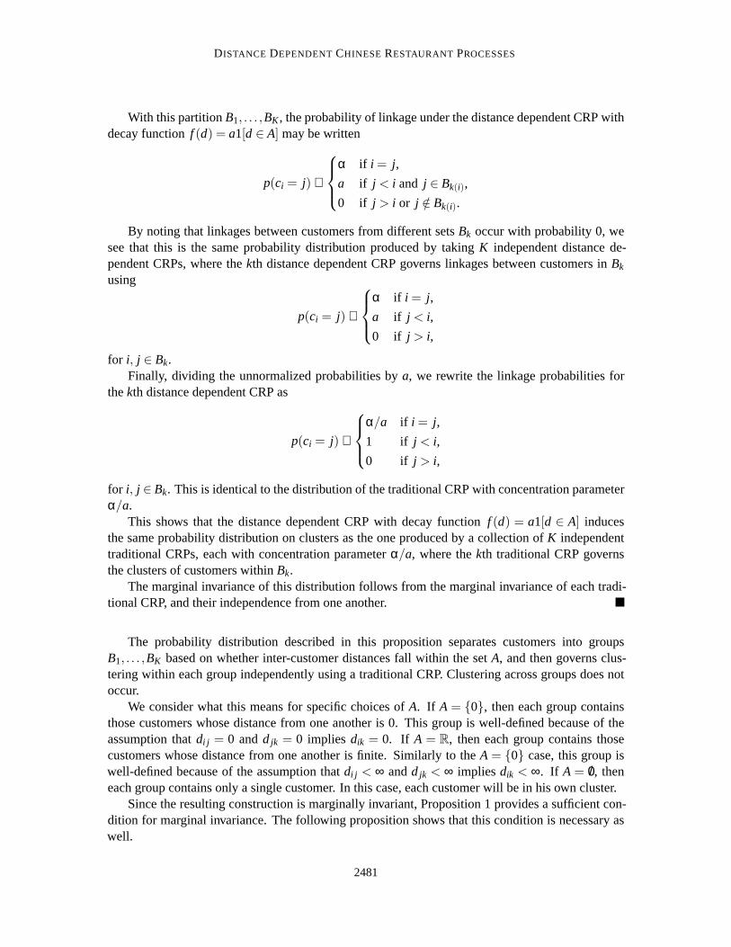
With this partitionB1, . . . ,BK , the probability of linkage under the distance dependent CRP withdecay functionf (d) = a1[d ∈ A] may be written

p(ci = j) ∝

α if i = j,

a if j < i and j ∈ Bk(i),

0 if j > i or j /∈ Bk(i).

By noting that linkages between customers from different setsBk occur with probability 0, wesee that this is the same probability distribution produced by takingK independent distance de-pendent CRPs, where thekth distance dependent CRP governs linkages between customers inBk

using

p(ci = j) ∝

α if i = j,

a if j < i,

0 if j > i,

for i, j ∈ Bk.Finally, dividing the unnormalized probabilities bya, we rewrite the linkage probabilities for

thekth distance dependent CRP as

p(ci = j) ∝

α/a if i = j,

1 if j < i,

0 if j > i,

for i, j ∈ Bk. This is identical to the distribution of the traditional CRP with concentration parameterα/a.

This shows that the distance dependent CRP with decay functionf (d) = a1[d ∈ A] inducesthe same probability distribution on clusters as the one produced by a collectionof K independenttraditional CRPs, each with concentration parameterα/a, where thekth traditional CRP governsthe clusters of customers withinBk.

The marginal invariance of this distribution follows from the marginal invariance of each tradi-tional CRP, and their independence from one another.

The probability distribution described in this proposition separates customersinto groupsB1, . . . ,BK based on whether inter-customer distances fall within the setA, and then governs clus-tering within each group independently using a traditional CRP. Clustering across groups does notoccur.

We consider what this means for specific choices ofA. If A = {0}, then each group containsthose customers whose distance from one another is 0. This group is well-defined because of theassumption thatdi j = 0 andd jk = 0 implies dik = 0. If A = R, then each group contains thosecustomers whose distance from one another is finite. Similarly to theA = {0} case, this group iswell-defined because of the assumption thatdi j < ∞ andd jk < ∞ implies dik < ∞. If A = /0, theneach group contains only a single customer. In this case, each customer willbe in his own cluster.

Since the resulting construction is marginally invariant, Proposition 1 providesa sufficient con-dition for marginal invariance. The following proposition shows that this condition is necessary aswell.

2481

BLEI AND FRAZIER

Proposition 2 If the distance dependent CRP for a given decay function f is marginally invariantover all sets of sequential distances then f is of the form f(d) = a1[d ∈ A] for some a> 0 and Aequal to either/0, {0}, or R.

Proof Consider a setting with 3 customers, in which customer 2 may either be absent, orpresentwith his seating assignment marginalized out. Fix a non-increasing decay function f with f (∞) = 0and suppose that the distances are sequential, sod13 = d23 = d12 = ∞. Suppose that the distance de-pendent CRP resulting from thisf and any collection of sequential distances is marginally invariant.Then the probability that customers 1 and 3 share a table must be the same whether customer 2 isabsent or present.

If customer 2 is absent,

P{1 and 3 sit at same table| 2 absent}= f (d31)

f (d31)+α. (4)

If customer 2 is present, customers 1 and 3 may sit at the same table in two different ways: 3sits with 1 directly (c3 = 1); or 3 sits with 2, and 2 sits with 1 (c3 = 2 andc2 = 1). Thus,

P{1 and 3 sit at same table| 2 present}

=f (d31)

f (d31)+ f (d32)+α+

(

f (d32)

f (d31)+ f (d32)+α

)(

f (d21)

f (d21)+α

)

. (5)

For the distance dependent CRP to be marginally invariant, Equation (4) andEquation (5) mustbe identical. Writing Equation (4) on the left side and Equation (5) on the right,we have

f (d31)

f (d31)+α=

f (d31)

f (d31)+ f (d32)+α+

(

f (d32)

f (d31)+ f (d32)+α

)(

f (d21)

f (d21)+α

)

. (6)

We now consider two different possibilities for the distancesd32 andd21, always keepingd31 =d21+d32.

First, supposed21 = 0 andd32 = d31 = d for somed ≥ 0. By multiplying Equation (6) throughby (2 f (d)+α)( f (0)+α)( f (d)+α) and rearranging terms, we obtain

0= α f (d)( f (0)− f (d)) .

Thus, eitherf (d) = 0 or f (d) = f (0). Since this is true for eachd ≥ 0 and f is nonincreasing,f = a1[d ∈ A] with a≥ 0 and eitherA= /0, A=R, A= [0,b], or A= [0,b) with b∈ [0,∞). BecauseA= /0 is among the choices, we may assumea> 0 without loss of generality. We now show that ifA= [0,b] or A= [0,b), then we must haveb= 0 andA is of the form claimed by the proposition.

Suppose for contradiction thatA= [0,b] or A= [0,b) with b> 0. Consider distances given byd32 = d21 = d = b− ε with ε ∈ (0,b/2). By multiplying Equation (5) through by

( f (2d)+ f (d)+α)( f (d)+α)( f (2d)+α)

and rearranging terms, we obtain

0= α f (d)( f (d)− f (2d)) .

2482


Since f (d) = a> 0, we must havef (2d) = f (d)> 0. But, 2d = 2(b−ε)> b implies together withf (2d) = a1[2d ∈ A] that f (2d) = 0, which is a contradiction.

These two propositions are combined in the following corollary, which states that the class ofdecay functions considered in Propositions 1 and 2 is both necessary and sufficient for marginalinvariance.

Corollary 3 Fix a particular decay function f . The distance dependent CRP resulting from thisdecay function is marginally invariant over all sequential distances if and only if f is of the formf (d) = a1[d ∈ A] for some a> 0 and some A∈ { /0,{0},R}.

Proof Sufficiency for marginal invariance is shown by Proposition 1. Necessityis shown by Propo-sition 2.

Although Corollary 3 allows any choice ofa > 0 in the decay functionf (d) = a1[d ∈ A], thedistribution of the distance dependent CRP with a particularf andα remains unchanged if bothf andα are multiplied by a constant factor (see Equation (2)). Thus, the distance dependent CRPdefined byf (d) = a1[d∈A] and concentration parameterα is identical to the one defined byf (d) =1[d∈A] and concentration parameterα/a. In this sense, we can restrict the choice ofa in Corollary 3(and also Propositions 1 and 2) toa= 1 without loss of generality.

A.2 General Distances

We now consider all sets of distances, including non-sequential distances. The class of distance de-pendent CRPs that are marginally invariant over this larger class of distances is even more restrictedthan in the sequential case. We have the following proposition providing a necessary condition formarginal invariance.

Proposition 4 If the distance dependent CRP for a given decay function f is marginally invariantover all sets of distances, both sequential and non-sequential, then f is identically0.

Proof From Proposition 2, we have that any decay function that is marginally invariant under allsequential distances must be of the formf (d) = a1[d ∈ A], wherea> 0 andA∈ { /0,{0},R}. Wenow show that if the decay function is marginally invariant underall sets of distances (not just thosethat are sequential), thenf (0) = 0. The only decay function of the formf (d) = a1[d ∈ A] thatsatisfiesf (0) = 0 is the one that is identically 0, and so this will show our result.

To show f (0) = 0, suppose that we haven+1 customers, all of whom are a distance 0 awayfrom one another, sodi j = 0 for i, j = 1, . . . ,n+1. Under our assumption of marginal invariance,the probability that the firstn customers sit at separate tables should be invariant to the absence orpresence of customern+1.

When customern+1 is absent, the only way in which the firstn customers may sit at separatetables is for each to link to himself. Letpn = α/(α+(n−1) f (0)) denote the probability of a givencustomer linking to himself when customern+1 is absent. Then

P{1, . . . ,n sit separately| n+1 absent}= (pn)n. (7)

2483

BLEI AND FRAZIER

We now consider the case when customern+1 is present. Letpn+1 = α/(α+n f(0)) be theprobability of a given customer linking to himself, and letqn+1 = f (0)/(α+n f(0)) be the proba-bility of a given customer linking to some other given customer. The firstn customers may eachsit at separate tables in two different ways. First, each may link to himself, which occurs withprobability (pn+1)

n. Second, all but one of these firstn customers may link to himself, with theremaining customer linking to customern+1, and customern+1 linking either to himself or to thecustomer that linked to him. This occurs with probabilityn(pn+1)

n−1qn+1(pn+1+qn+1). Thus, thetotal probability that the firstn customers sit at separate tables is

P{1, . . . ,n sit separately| n+1 present}= (pn+1)n+n(pn+1)

n−1qn+1(pn+1+qn+1). (8)

Under our assumption of marginal invariance, Equation (7) must be equalto Equation (8), andso

0= (pn+1)n+n(pn+1)

n−1qn+1(pn+1+qn+1)− (pn)n. (9)

Considern = 2. By substituting the definitions ofp2, p3, andq3, and then rearranging terms,we may rewrite Equation (9) as

0=α f (0)2(2 f (0)2−α2)

(α+ f (0))2(α+2 f (0))3 ,

which is satisfied only whenf (0) ∈ {0,α/√

2}. Consider the second of these roots,α/√

2. Whenn = 3, this value off (0) violates Equation (9). Thus, the first root is the only possibility and wemust havef (0) = 0.

The decay functionf = 0 described in Proposition 4 is a special case of the decay function fromProposition 2, obtained by takingA= /0. As described above, the resulting probability distributionis one in which each customer links to himself, and is thus clustered by himself. This distribution ismarginally invariant. From this observation quickly follows the following corollary.

Corollary 5 The decay function f= 0 is the only one for which the resulting distance dependentCRP is marginally invariant over all distances, both sequential and non-sequential.

Proof Necessity off = 0 for marginal invariance follows from Proposition 4. Sufficiency followsfrom the fact that the probability distribution on partitions induced byf = 0 is the one under whicheach customer is clustered alone almost surely, which is marginally invariant.

Appendix B. Gibbs Sampling for the Hyperparameters

To enhance our models, we place a prior on the concentration parameterα and augment our Gibbssampler accordingly, just as is done in the traditional CRP mixture (Escobar and West, 1995). Tosample from the posterior ofα given the customer assignmentsc and data, we begin by notingthatα is conditionally independent of the observed data given the customer assignments. Thus, thequantity needed for sampling is

p(α |c) ∝ p(c |α)p(α),

2484


wherep(α) is a prior on the concentration parameter.From the independence of theci under the generative process,p(c |α) = ∏N

i=1 p(ci |D,α). Nor-malizing provides

p(c |α) =N

∏i=1

1[ci = i]α+1[ci 6= i] f (dici )

α+∑ j 6=i f (di j )

∝ αK

[

N

∏i=1

(

α+∑j 6=i

f (di j )

)]−1

,

whereK is the number of self-linksci = i in the customer assignmentsc. AlthoughK is equal to thenumber of tables|z(c)| when distances are sequential,K and|z(c)| generally differ when distancesare non-sequential. Then,

p(α |c) ∝ αK

[

N

∏i=1

(

α+∑j 6=i

f (di j )

)]−1

p(α). (10)

Equation (10) reduces further in the following special case:f is the window decay function,f (d) = 1[d < a]; di j = i − j for i > j; and distances are sequential sodi j = ∞ for i < j. In this case,∑i−1

j=1 f (di j ) = (i−1)∧ (a−1), where∧ is the minimum operator, and

N

∏i=1

(

α+i−1

∑j=1

f (di j )

)

= (α+a−1)[N−a]+Γ(α+a∧N)/Γ(α), (11)

where[N−a]+ = max(0,N−a) is the positive part ofN−a. Then,

p(α |c) ∝Γ(α)

Γ(α+a∧N)

αK

(α+a−1)[N−a]+p(α).

If we use the identity decay function, which results in the traditional CRP, thenwe recover anexpression from Antoniak (1974):p(α |c) ∝ Γ(α)

Γ(α+N)αK p(α). This expression is used in Escobar

and West (1995) to sample exactly from the posterior ofα when the prior is gamma distributed.In general, if the prior onα is continuous then it is difficult to sample exactly from the posterior

of Equation (10). There are a number of ways to address this. We may, for example, use the Griddy-Gibbs method (Ritter and Tanner, 1992). This method entails evaluating Equation (10) on a finite setof points, approximating the inverse cdf ofp(α |c) using these points, and transforming a uniformrandom variable with this approximation to the inverse cdf.

We may also sample over any hyperparameters in the decay function used (e.g., the window sizein the window decay function, or the rate parameter in the exponential decayfunction) within ourGibbs sampler. For the rest of this section, we usea to generically denote a hyperparameter in thedecay function, and we make this dependence explicit by writingf (d,a).

To describe Gibbs sampling over these hyperparameters in the decay function, we first write

p(c | α,a) =N

∏i=1

1[ci = i]α+1[ci 6= i] f (dici ,a)

α+∑i−1j=1 f (di j ,a)

= αK

[

∏i:ci 6=i

f (di j ,a)

][

N

∏i=1

(

α+i−1

∑j=1

f (di j ,a)

)]−1

.

2485

BLEI AND FRAZIER

Sincea is conditionally independent of the observed data givenc andα, to sample overa in ourGibbs sampler it is enough to know the density

p(a | c,α) ∝

[

∏i:ci 6=i

f (di j ,a)

][

N

∏i=1

(

α+i−1

∑j=1

f (di j ,a)

)]−1

p(a | α). (12)

In many cases our priorp(a | α) ona will not depend onα.In the case of the window decay function with sequential distances anddi j = i − j for i > j, we

can simplify this further as we did above with Equation (11). Noting that∏i:ci 6=i f (di j ,a) will be 1for thosea> maxi i−ci , and 0 for othera, we have

p(a | c,α) ∝Γ(α)

Γ(α+a∧N)

p(a | α)1[a> maxi i−ci ]

(α+a−1)[N−a]+.

If the prior distribution ona is discrete and concentrated on a finite set, as it might be with thewindow decay function, one can simply evaluate and normalize Equation (12)on this set. If theprior is continuous, as it might be with the exponential decay function, then itis difficult to sampleexactly from Equation (12), but one can again use the Griddy-Gibbs approach of Ritter and Tanner(1992) to sample approximately.

References

A. Ahmed and E. Xing. Dynamic non-parametric mixture models and the recurrent Chinese restau-rant process with applications to evolutionary clustering. InInternational Conference on DataMining, 2008.

C. Antoniak. Mixtures of Dirichlet processes with applications to Bayesian nonparametric problems.The Annals of Statistics, 2(6):1152–1174, 1974.

D. Blackwell. Discreteness of Ferguson selections.The Annals of Statistics, 1(2):356–358, 1973.

D. Blei and P. Frazier. Distance dependent Chinese restaurant processes. InInternational Confer-ence on Machine Learning, 2010.

D. Blei and M. Jordan. Variational inference for Dirichlet process mixtures. Journal of BayesianAnalysis, 1(1):121–144, 2005.

D. Blei, T. Griffiths, and M. Jordan. The nested Chinese restaurant process and Bayesian nonpara-metric inference of topic hierarchies.Journal of the ACM, 57(2):1–30, 2010.

D.B. Dahl. Distance-based probability distribution for set partitions with applications to Bayesiannonparametrics. InJSM Proceedings. Section on Bayesian Statistical Science, American Statisti-cal Association, Alexandria, Va, 2008.

H. Daume. Fast search for Dirichlet process mixture models. InArtificial Intelligence and Statistics,San Juan, Puerto Rico, 2007. URLhttp://pub.hal3.name/#daume07astar-dp .

J. Duan, M. Guindani, and A. Gelfand. Generalized spatial Dirichlet process models.Biometrika,94:809–825, 2007.

2486


D. Dunson. Bayesian dynamic modeling of latent trait distributions.Biostatistics, 2006.

D. Dunson, N. Pillai, and J. Park. Bayesian density regression.Journal of the Royal StatisticalSociety: Series B (Statistical Methodology), 69(2):163–183, 2007.

M. Escobar and M. West. Bayesian density estimation and inference using mixtures.Journal of theAmerican Statistical Association, 90:577–588, 1995.

T. Ferguson. A Bayesian analysis of some nonparametric problems.The Annals of Statistics, 1:209–230, 1973.

E. Fox, E. Sudderth, M. Jordan, and A. Willsky. Developing a tempered HDP-HMM for systemswith state persistence. Technical report, MIT Laboratory for Information and Decision Systems,2007.

C. Geyer and E. Thompson. Constrained Monte Carlo maximum likelihood for dependent data.Journal of the American Statistical Association, 54(657–699), 1992.

S. Goldwater, T. Griffiths, and M. Johnson. Interpolating between typesand tokens by estimatingpower-law generators. InNeural Information Processing Systems, 2006.

J. Griffin and M. Steel. Order-based dependent Dirichlet processes. Journal of the American Statis-tical Association, 101(473):179–194, 2006.

J.A. Hartigan. Partition models.Communications in Statistics-Theory and Methods, 19(8):2745–2756, 1990.

M. Johnson, T. Griffiths, and Goldwater S. Adaptor grammars: A framework for specifying com-positional nonparametric Bayesian models. In B. Scholkopf, J. Platt, and T. Hoffman, editors,Advances in Neural Information Processing Systems 19, pages 641–648, Cambridge, MA, 2007.MIT Press.

R. Kass and A. Raftery. Bayes factors.Journal of the American Statistical Association, 90(430):773–795, 1995.

W. Li, D. Blei, and A. McCallum. Nonparametric Bayes pachinko allocation. InThe 23rd Confer-ence on Uncertainty in Artificial Intelligence, 2007.

P. Liang, M. Jordan, and B. Taskar. A permutation-augmented sampler for DP mixture models. InInternational Conference on Machine Learning, 2007.

S. MacEachern. Dependent nonparametric processes. InASA Proceedings of the Section onBayesian Statistical Science, 1999.

A. McCallum, K. Nigam, J. Rennie, and K. Seymore. Automating the constructionof internetportals with machine learning.Information Retrieval, 2000.

K.T. Miller, T.L. Griffiths, and M.I. Jordan. The phylogenetic indian buffet process: A non-exchangeable nonparametric prior for latent features. In David A. McAllester and Petri Myl-lymaki, editors,UAI, pages 403–410. AUAI Press, 2008.

2487

BLEI AND FRAZIER

P. Mueller and F. Quintana. Random partition models with regression on covariates. InInternationalConference on Interdisciplinary Mathematical and Statistical Techniques, 2008.

P. Muller, F. Quintana, and G. Rosner. Bayesian clustering with regression. Working paper, 2008.

R. Neal. Probabilistic inference using Markov chain Monte Carlo methods. Technical Report CRG-TR-93-1, Department of Computer Science, University of Toronto, 1993.

R. Neal. Markov chain sampling methods for Dirichlet process mixture models.Journal of Compu-tational and Graphical Statistics, 9(2):249–265, 2000.

J. Pitman. Combinatorial Stochastic Processes. Lecture Notes for St. Flour Summer School.Springer-Verlag, New York, NY, 2002.

C. Rasmussen and Z. Ghahramani. Infinite mixtures of Gaussian process experts. In T. Dietterich,S. Becker, and Z. Ghahramani, editors,Advances in Neural Information Processing Systems 14,Cambridge, MA, 2002. MIT Press.

C. Ritter and M. Tanner. Facilitating the Gibbs sampler: The Gibbs stopper and the Griddy-Gibbssampler.Journal of the American Statistical Association, 87(419):861–868, 1992.

C. Robert and G. Casella.Monte Carlo Statistical Methods. Springer Texts in Statistics. Springer-Verlag, New York, NY, 2004.

E. Sudderth, A. Torralba, W. Freeman, and A. Willsky. Describing visual scenes using transformedDirichlet processes. InAdvances in Neural Information Processing Systems 18, 2005.

E.B. Sudderth and M. I. Jordan. Shared segmentation of natural scenes using dependent pitman-yorprocesses. In Daphne Koller, Dale Schuurmans, Yoshua Bengio, andLeon Bottou, editors,NIPS,pages 1585–1592. MIT Press, 2008.

Y. Teh. A hierarchical Bayesian language model based on Pitman-Yor processes. InProceedingsof the Association of Computational Linguistics, 2006.

Y. Teh, M. Jordan, M. Beal, and D. Blei. Hierarchical Dirichlet processes.Journal of the AmericanStatistical Association, 101(476):1566–1581, 2006.

E. Xing, M. Jordan, and R. Sharan. Bayesian haplotype inference viathe Dirichlet process.Journalof Computational Biology, 14(3):267–284, 2007.

Y. Xue, D. Dunson, and L. Carin. The matrix stick-breaking process for flexible multi-task learning.In International Conference on Machine Learning, 2007.

X. Zhu, Z. Ghahramani, and J. Lafferty. Time-sensitive Dirichlet process mixture models. TechnicalReport CMU-CALD-05-104, Carnegie Mellon University, 2005.

2488

Distance Dependent Chinese Restaurant Processes

Documents

Transcript of Distance Dependent Chinese Restaurant Processes