DISTANCE BETWEEN A MAXIMUM MODULUS POINT AND THE ZERO SET ... · DISTANCE BETWEEN A MAXIMUM MODULUS...
80
DISTANCE BETWEEN A MAXIMUM MODULUS POINT AND THE ZERO SET OF AN ENTIRE FUNCTION a dissertation submitted to the department of mathematics and the institute of engineering and science of bilkent university in partial fulfillment of the requirements for the degree of doctor of philosophy By Adem Ersin ¨ Ureyen November, 2006
Transcript of DISTANCE BETWEEN A MAXIMUM MODULUS POINT AND THE ZERO SET ... · DISTANCE BETWEEN A MAXIMUM MODULUS...

DISTANCE BETWEEN A MAXIMUMMODULUS POINT AND THE ZERO SET OF
AN ENTIRE FUNCTION
a dissertation submitted to
the department of mathematics
and the institute of engineering and science
of bilkent university
in partial fulfillment of the requirements
for the degree of
doctor of philosophy
By
Adem Ersin Ureyen
November, 2006
I certify that I have read this thesis and that in my opinion it is fully adequate,
in scope and in quality, as a dissertation for the degree of doctor of philosophy.
Assoc. Prof. Dr. H. Turgay Kaptanoglu (Supervisor)
I certify that I have read this thesis and that in my opinion it is fully adequate,
in scope and in quality, as a dissertation for the degree of doctor of philosophy.
Asst. Prof. Dr. Secil Gergun
I certify that I have read this thesis and that in my opinion it is fully adequate,
in scope and in quality, as a dissertation for the degree of doctor of philosophy.
Assoc. Prof. Dr. Aurelian Gheondea
ii

I certify that I have read this thesis and that in my opinion it is fully adequate,
in scope and in quality, as a dissertation for the degree of doctor of philosophy.
Assoc. Prof. Dr. Tugrul Hakioglu
I certify that I have read this thesis and that in my opinion it is fully adequate,
in scope and in quality, as a dissertation for the degree of doctor of philosophy.
Assoc. Prof. Dr. A. Sinan Sertoz
Approved for the Institute of Engineering and Science:
Prof. Dr. Mehmet B. BarayDirector of the Institute
iii

ABSTRACT
DISTANCE BETWEEN A MAXIMUM MODULUSPOINT AND THE ZERO SET OF AN ENTIRE
FUNCTION
Adem Ersin Ureyen
Ph.D. in Mathematics
Supervisor: Assoc. Prof. Dr. H. Turgay Kaptanoglu
November, 2006
We obtain asymptotical bounds from below for the distance between a maximum
modulus point and the zero set of an entire function. Known bounds (Macintyre,
1938) are more precise, but they are valid only for some maximum modulus
points. Our bounds are valid for all maximum modulus points and moreover, up
to a constant factor, they are unimprovable.
We consider entire functions of regular growth and obtain better bounds for
these functions. We separately study the functions which have very slow growth.
We show that the growth of these functions can not be very regular and obtain
precise bounds for their growth irregularity.
Our bounds are expressed in terms of some smooth majorants of the growth
function. These majorants are defined by using orders, types, (strong) proximate
orders of entire functions.
Keywords: Entire function, Maximum modulus point, Zero set, Order, Type,
Proximate order, Regular growth.
iv
OZET
BIR TUM FONKSIYONUN BIR MAKSIMUM MODULNOKTASI ILE SIFIR KUMESI ARASINDAKI UZAKLIK
Adem Ersin Ureyen
Matematik, Doktora
Tez Yoneticisi: Doc. Dr. H. Turgay Kaptanoglu
Kasım, 2006
Bir tum fonksiyonun maksimum modul noktası ile sıfır kumesi arasındaki uzaklık
icin asagıdan asimptotik sınır buluyoruz. Bilinen sınırlar (Macintyre, 1938) daha
kesin, ama sadece bazı maksimum modul noktaları icin gecerli. Buldugumuz
sonuclar tum maksimum modul noktaları icin gecerli ve bir sabit carpan haricinde
iyilestirilemez.
Ek olarak, duzenli buyuyen tum fonksiyonları inceliyoruz ve bu tip fonksiyon-
lar icin daha iyi sınırlar buluyoruz. Cok yavas buyuyen tum fonksiyonları ayrıca
inceliyor, bu fonksiyonların cok duzenli buyuyemeyecegini gosteriyor ve buyume
duzensizlikleri hakkında kesin sınırlar buluyoruz.
Buldugumuz sonuclar buyume fonksiyonunun bazı duzgun ust sınırları cinsin-
den ifade edilmistir. Bu ust sınırlar tum fonksiyonların mertebeleri, tipleri ve
(kuvvetli) yaklasık mertebeleri kullanılarak tanımlanır.
Anahtar sozcukler : Tum fonksiyon, Maksimum modul noktası, Sıfır kumesi, Mer-
tebe, Tip, Yaklasık mertebe, Kuvvetli yaklasık mertebe, Duzenli buyume.
v

Acknowledgement
The true supervisor of this thesis is Iossif V. Ostrovskii. He proposed the
problem, and the thesis is completed wholly under his supervision. For adminis-
trative reasons, the supervisor had to be present at the defense. I. V. Ostrovskii’s
duties were performed by H. T. Kaptanoglu during the defense as he was unable
to attend it and H. T. Kaptanoglu’s name was written as supervisor on the final
copy of the thesis.
I would like to express my deep gratitude to my supervisor Prof. I. V. Os-
trovskii for his excellent guidance, valuable suggestions, encouragements, and
patience.
I would like to thank H. T. Kaptanoglu and Secil Gergun for careful reading
of the text and valuable remarks.
I would like to thank the jury members for serving on the thesis committee.
Finally, I would like to thank my family and friends for their encouragements
and supports.
vi

Contents
1 Introduction 1
2 Main Definitions 4
2.1 Order and Type of an Entire Function . . . . . . . . . . . . . . . 4
2.2 Proximate Orders . . . . . . . . . . . . . . . . . . . . . . . . . . . 7
2.3 Strong Proximate Orders . . . . . . . . . . . . . . . . . . . . . . . 11
2.4 Admissible and Strongly Admissible Proximate Orders . . . . . . 12
3 Statement of Results 14
3.1 Distance between a maximum modulus point and the zero set of
an entire function without assumption of regular growth . . . . . 15
3.2 Distance between a maximum modulus point and the zero set of
an entire function with assumption of regular growth . . . . . . . 17
3.3 Growth irregularity of slowly growing entire functions . . . . . . . 22
4 Preliminaries 26
5 Auxiliary Results 34
vii
CONTENTS viii
5.1 Properties of proximate orders . . . . . . . . . . . . . . . . . . . . 34
5.2 Properties of strong proximate orders . . . . . . . . . . . . . . . . 38
6 Proof of Theorem 1 41
7 Proof of Theorem 2 48
8 Proof of Theorem 3 53
9 Proof of Theorem 4 61

Chapter 1
Introduction
A function f : C → C which is analytic in the whole complex plane is called an
entire function. It can be represented by an everywhere convergent power series,
f(z) =∞∑
k=0
ckzk, z ∈ C.
In the above series, if only finitely many of the coefficients cn are nonzero, then
f is called a polynomial. Otherwise it is called transcendental.
To characterize the asymptotic behavior of an entire function f , we introduce
the growth function
M(r, f) := max|z|=r
|f(z)|. (1.1)
It follows from the maximum modulus principle that M(r, f) is a nondecreasing
function of r ∈ R+. If f is not constant, then M(r, f) strictly increases and tends
to ∞ as r →∞.
Let f be a polynomial of degree n,
f(z) =n∑
k=0
ckzk, cn 6= 0.
It can be easily shown that
limr→∞
log M(r, f)
log r= n.
1

CHAPTER 1. INTRODUCTION 2
Furthermore, f has exactly n zeros in C. This shows that there is a close connec-
tion between the asymptotic behavior and the set of zeros of a polynomial. The
main subject matter of the entire function theory is to establish relations between
the growth of an entire function and the distribution of its zeros (see, e.g., [7],
[10], [11]). The aim of this work is to obtain such a relation: We investigate the
distance between the zero set of an entire function and points where the function
is “large” in the sense we will describe below.
For each r > 0, there are points on the circle z : |z| = r where the maximum
in (1.1) is attained. We will denote such a point by w and call it a maximum
modulus point. Equivalently, a point w is a maximum modulus point if
|f(w)| = M(|w|, f).
We denote by Zf the zero set of the entire function f , i.e., Zf = z : f(z) = 0.For each maximum modulus point w, we denote by R(w, f) the distance between
w and Zf ,
R(w, f) := inf|w − z| : f(z) = 0.
The aim of this work is to obtain asymptotic (as |w| → ∞) bounds for R(w, f)
from below. The first results in this direction were obtained by A.J. Macintyre.
Theorem A ([12]) (i) The following inequality holds
lim sup|w|→∞
1
|w|R(w, f)(log M(|w|, f))1/2 > 0. (1.2)
(ii) For each ε > 0 the following inequality holds
lim inf|w|→∞|w|/∈Aε
1
|w|R(w, f)(log M(|w|, f))12+ε > 0, (1.3)
where Aε ⊂ R+ is such that∫
Aε
dt
t< ∞. (1.4)
The inequality (1.2) gives an asymptotic bound for R(w, f) from below only
on a sequence of values of |w| → ∞. The inequality (1.3) gives a little less

CHAPTER 1. INTRODUCTION 3
precise bound that is valid outside of a “small” set. The following problem arises:
To obtain bounds for R(w, f) from below that are valid for all sufficiently large
values of |w|. Main results of this work (see Theorem 1, Theorem 2 below) give
such bounds.
Note that the bounds in (1.2)-(1.3) are inversely related to the growth of f :
the slower the growth of f is, the better the bounds are. One significance of
Theorem A is that its results are directly in terms of M(r, f). Our results, on the
other hand, are in terms of some “smooth majorants” of M(r, f). We will explain
the meaning of “smooth majorant” in Chapter 2.
The results of this dissertation have been published in [15], [16], [18], and will
be published in [13], [14].

Chapter 2
Main Definitions
2.1 Order and type of an entire function
To measure the growth of an entire function f , we consider a class of “simple”
and “smooth” functions and compare M(r, f) with the elements of this class. In
this and the following sections we will describe some special classes of comparison
functions that are commonly used in the entire function theory.
It is easy to see that if an entire function f satisfies
lim infr→∞
M(r, f)
rn< ∞,
for some positive integer n, then f is a polynomial of degree at most n. Therefore,
to measure the growth of transcendental (non-polynomial) entire functions it is
necessary to use comparison functions that grow faster than powers of r. In entire
function theory most commonly used comparison functions are of the form
erk
, k > 0.
An entire function f is said to be of finite order if there exists a positive
constant k such that the inequality
M(r, f) < erk
(2.1)
4

CHAPTER 2. MAIN DEFINITIONS 5
holds asymptotically, i.e., for all sufficiently large values of r. The order (or the
order of growth) of an entire function f is the greatest lower bound of those values
of k for which inequality (2.1) is asymptotically valid. We denote the order of an
entire function by ρ = ρf . Hence
ρ = inf k : M(r, f) < erk
for r > rk.
It follows from the above definition that if f is an entire function of order ρ,
and if ε is an arbitrary positive number, then
erρ−ε
< M(r, f) < erρ+ε
, (2.2)
where the inequality on the left is satisfied for some sequence rn tending to infinity
and the inequality on the right is satisfied for all sufficiently large values of r. By
taking logarithms twice, we obtain from (2.2) that
ρ = lim supr→∞
log log M(r, f)
log r. (2.3)
Examples.
1. Let f(z) = ezn, n ∈ N. Then M(r, f) = ern
, and using (2.3) we see that
ρf = n.
2. Let
f(z) = sin z =∞∑
k=0
(−1)kz2k+1
(2k + 1)!.
Then M(r, f) = (er − e−r)/2 and ρf = 1.
3. Let
f(z) =sin√
z√z
=∞∑
k=0
(−1)kzk
(2k + 1)!.
Then M(r, f) = (e√
r − e−√
r)/(2√
r) and ρf = 12.
4. Let
f(z) =∞∏
k=1
(1 +
( z
ek4
)k3)
.
CHAPTER 2. MAIN DEFINITIONS 6
It can be shown that (see the proof of Theorem 3 below)
log M(r, f) =1
2log2 r + O(log3/2 r).
Then, by (2.3), ρf = 0.
5. Let f(z) = eez. Then M(r, f) = eer
and ρf = ∞.
Note that among the functions that have the same order, there are functions
that grow in different ways. For example, it is possible to construct entire func-
tions f1, f2, f3 such that
M(r, f1) ∼ er/ log r, M(r, f2) ∼ er, M(r, f3) ∼ er log r.
Although each of these functions has order 1, their asymptotical growth is appar-
ently different. To distinguish functions that have the same order, we use another
characteristic, the type.
An entire function f of order ρ is said be of finite type if there exists a positive
constant A such that the inequality
M(r, f) < eArρ
(2.4)
holds asymptotically. The greatest lower bound of those values of A for which
the inequality (2.4) is asymptotically fulfilled is called the type of f (with respect
to order ρ). We denote the type of an entire function f by σ = σf . Thus
σ = inf A : M(r, f) < eArρ
for r > rA.
It follows that if ε is an arbitrary positive number, then
e(σ−ε)rρ
< M(r, f) < e(σ+ε)rρ
, (2.5)
where the inequality on the left is satisfied for some sequence rn → ∞ and the
inequality on the right is satisfied for all sufficiently large values of r. After taking
a logarithm, we obtain from (2.5) that
σ = lim supr→∞
log M(r, f)
rρ.
If σf = 0, the function f is said to be of minimal type, if 0 < σf < ∞, of
normal type, and if σf = ∞, of maximal type.

CHAPTER 2. MAIN DEFINITIONS 7
Examples.
1. Let f(z) = eσzn, n ∈ N, 0 < σ < ∞. Then ρf = n and σf = σ.
2. Let M(r, f1) ∼ er/ log r. Then ρf1 = 1 and σf1 = 0: f1 is of minimal type.
3. Let M(r, f2) ∼ er. Then ρf2 = 1 and σf2 = 1: f2 is of normal type.
4. Let M(r, f3) ∼ er log r. Then ρf3 = 1 and σf3 = ∞: f3 is of maximal type.
2.2 Proximate orders
Order and type are the simplest and the most common notions used for measuring
the growth of entire functions. But they are rather coarse. That is, there are
entire functions which have the same order and type but grow in substantially
different ways. It follows from a theorem of Clunie and Kovari that (see Theorem
C, p. 18), there exists entire functions f1, f2, f3 such that
log M(r, f1) = rρ + O(1), r →∞; ρf1 = ρ; σf1 = 1
log M(r, f2) = rρ log r + O(1), r →∞; ρf2 = ρ; σf2 = ∞log M(r, f3) = rρ log2 r + O(1), r →∞; ρf3 = ρ; σf3 = ∞.
Observe that log M(r, f2)/ log M(r, f1) ∼ log r and these functions have different
types. On the other hand, it is also true that log M(r, f3)/ log M(r, f2) ∼ log r.
However, these functions have the same order and type, i.e., it is not possible to
distinguish them by using the usual order and type. Likewise, there exists entire
functions g1, g2, g3 such that
log M(r, g1) = rρ + O(1), r →∞; ρg1 = ρ; σg1 = 1
log M(r, g2) = rρ/ log r + O(1), r →∞; ρg2 = ρ; σg2 = 0
log M(r, g3) = rρ/ log2 r + O(1), r →∞; ρg3 = ρ; σg3 = 0.
Here, again, log M(r, g2)/ log M(r, g3) ∼ log r, but these functions have the
same order and type. It is easy to see that the problem is related to functions
that have either minimal or maximal type. To avoid this, it is necessary to use
CHAPTER 2. MAIN DEFINITIONS 8
larger class of comparison functions than functions of the form eσrρand make all
functions of normal type. This can be done by using proximate orders introduced
by Valiron at the beginning of the 20th century.
We will define proximate orders separately for each of the following three
cases: 0 < ρ < ∞, ρ = 0, and ρ = ∞.
Definition (Valiron). (Proximate order when 0 < ρ < ∞) A continuously
differentiable positive function ρ(r) on R+ is called a proximate order if it satisfies
the conditions
limr→∞
ρ(r) = ρ, 0 < ρ < ∞; (2.6)
limr→∞
rρ′(r) log r = 0. (2.7)
If the inequalities
0 < σf := lim supr→∞
log M(r, f)
rρ(r)< ∞, (2.8)
hold, then ρ(r) is called a proximate order of f and σf is called the type of f
with respect to the proximate order ρ(r).
We call rρ(r) a smooth majorant of log M(r, f) if (2.8) is satisfied.
Roughly speaking, by using proximate orders we can consider any function
as of normal type. Following examples make the point more clear. Note that
r(log c/ log r) = c. We assume 0 < ρ < ∞.
Examples.
1. Let ρ1(r) ≡ ρ. Evidently, ρ1 satisfies (2.6)-(2.7) and therefore is a proximate
order. If f1 is of order ρ and of normal type σ in the usual sense, then ρ1(r)
is a proximate order of f1 and σ is the corresponding type.
2. Let ρ2(r) = ρ + log log r/ log r. It is easy to see that ρ2 satisfies (2.6)-(2.7),
and rρ2(r) = rρ log r. So, if log M(r, f2) ∼ rρ log r, then f2 is of maximal
type in the usual sense, but it is of normal type with respect to ρ2(r).
3. Let ρ3(r) = ρ + 2 log log r/ log r. Then rρ3(r) = rρ log2 r. Hence, if
log M(r, f3) ∼ rρ log2 r, then f3 is of maximal type in the usual sense,

CHAPTER 2. MAIN DEFINITIONS 9
but it is of normal type with respect to ρ3(r).
Note that ρ2(r) is not a proximate order of f3 and ρ3(r) is not a proximate
order of f2.
4. Let ρ4(r) = ρ − m log log log r/ log r. Then rρ4(r) = rρ/ logm(log r). If
log M(r, f4) ∼ rρ/ logm(log r), then f4 is of minimal type in usual sense,
but it is of normal type with respect to ρ4(r).
Remark. Proximate order of an entire function f is not uniquely determined.
If ρ(r) is a proximate order of f and σ is the corresponding type, then ρ(r) =
ρ(r) + log c/ log r is also a proximate order of f with corresponding type σ/c.
Valiron’s theorem (see [10, p. 35]) shows that proximate orders form a scale
of growth of entire functions of finite and positive order in the following sense:
For each entire function f of order ρ, 0 < ρ < ∞, there exists a proximate order
ρ(r) → ρ such that (2.8) holds.
The definition of proximate order for functions of order ρ, 0 < ρ < ∞, is well
known and generally accepted. The situation is different for functions of zero or
infinite order. For our purposes the following definitions are suitable.
In the case ρ = 0 the definition below is close to that of Levin [10, Ch. 1] but
contains more restrictions.
Definition (Proximate order when ρ = 0.) We call a function ρ(r), r ∈ R+, a
zero proximate order if it is representable in the form
ρ(r) =ϑ(log r)
log r, r ≥ r0 > 1,
where ϑ(x) ∈ C1(R+) is a positive concave function such that
limx→∞
eϑ(x)
x= ∞ and lim
x→∞ϑ(x)
x= 0. (2.9)
The class of zero proximate orders is sufficient for measuring the growth of all
transcendental entire functions of order zero. That is, for every entire function f
of order zero, there exists a zero proximate order such that (2.8) holds (see [10,
p. 35].)

CHAPTER 2. MAIN DEFINITIONS 10
Example. Let ρ(r) = n log log r/ log r, n > 1. Then ρ(r) is a zero proximate
order with ϑ(x) = n log x. If f is an entire function such that log M(r, f) ∼(log r)n, then f is of order zero and of maximal type in the usual sense, but it is
of normal type with respect to ρ(r).
For functions of infinite order we will use the following definition which is
based on the results of Earl and Hayman [4].
Definition (Proximate order when ρ = ∞.) We call a function ρ(r), r ∈ R+, an
infinite proximate order if it is representable in the form
ρ(r) =ϑ(log r)
log r, r ≥ r0 > 1,
where ϑ(x) ∈ C2(R+) is a positive convex function such that
limx→∞
ϑ′(x) = ∞, and limx→∞
ϑ′′(x)
ϑ′2(x)= 0. (2.10)
It is proved in [4] that for every entire function f of infinite order there exists
an infinite proximate order such that (2.8) holds. That is, the class of infinite
proximate orders is sufficient for measuring the growth of entire functions of
infinite order.
Example. Let ρ(r) = r/ log r. Then ρ(r) is an infinite proximate order with
ϑ(x) = ex. If f is an entire function such that log M(r, f) ∼ er, then ρ(r) is a
proximate order of f.
Using proximate orders is not the only way of measuring the growth of en-
tire functions. For some applications, it is necessary to use functions that have
smoother behavior than required by equations (2.6)-(2.7), (2.9), and (2.10).
In the remaining sections of this chapter we will describe some subclasses of
proximate orders that we will need for our purposes.

CHAPTER 2. MAIN DEFINITIONS 11
2.3 Strong proximate orders
A strong proximate order, introduced by Levin in the 1950′s of 20th century (see
[10, Ch. 1], is a twice continuously differentiable proximate order that satisfies
the additional conditions stated below. Strong proximate orders form a proper
subclass of proximate orders; nevertheless, they too are sufficient for complete
characterization of the growth of entire functions.
As before we will define strong proximate orders separately for each of the
following cases: 0 < ρ < ∞, ρ = 0, ρ = ∞.
Definition (Levin) (Strong proximate order when 0 < ρ < ∞.) A strong
proximate order is a function ρ(r) ∈ C2(R+) representable in the form
ρ(r) = ρ +ϑ1(log r)− ϑ2(log r)
log r, r ≥ r0 > 1, (2.11)
where 0 < ρ < ∞, and ϑj, j = 1, 2, is a concave function of C2(R+) satisfying the
conditions
limx→∞
ϑj(x) = ∞, limx→∞
ϑj(x)
x= 0, lim
x→∞ϑ′′j (x)
ϑ′j(x)= 0. (2.12)
It is easy to check that any strong proximate order is a proximate order, i.e.,
satisfies (2.6)-(2.7).
For any strong proximate order ρ(r), if the inequality (2.8) is satisfied, then
we say that ρ(r) is a strong proximate order of f and σf is the corresponding
type. Given any entire function f of order ρ, 0 < ρ < ∞, there exists a strong
proximate order ρ(r) such that (2.8) holds. This is proved by Levin ([10, pp.
39–41].)
We note that if an entire function f has maximal type with respect to the
usual order ρ (i.e., if σ = lim supr→∞ log M(r, f)/rρ = ∞), then we can choose
ϑ2 ≡ 0 in (2.11). Likewise, if f has minimal type in the usual sense, then we can
choose ϑ1 ≡ 0. The first assertion immediately follows from the construction of
Levin. We will prove the second assertion later (see Lemma 4.2.)

CHAPTER 2. MAIN DEFINITIONS 12
Definition (Strong proximate order when ρ = 0.) We call a zero proximate order
ρ(r) = ϑ(log r)/ log r, a zero strong proximate order, if the following additional
condition is satisfied:
ϑ′′(x) + ϑ′2(x) > 0, x ≥ x0 > 0. (2.13)
Instead of (2.13), Levin uses the slightly weaker condition ϑ′′(x)/ϑ′(x) → 0,
x → ∞. We will need (2.13) to guarantee that the function rρ(r) = eϑ(log r) is
convex with respect to log r.
We will prove later (see Lemma 4.3) that any entire function of order zero has
a zero strong proximate order.
When ρ = ∞, we will call an infinite proximate order also as an infinite strong
proximate order.
2.4 Admissible and strongly admissible proxi-
mate orders
Later it will be necessary for us to consider separately the class of entire functions
that satisfy
lim supr→∞
log M(r, f)
log2 r= ∞. (2.14)
To measure the growth of such entire functions in addition to to proximate and
strong proximate orders, we will also use the following subclass of strong proxi-
mate orders.
Definition. For 0 < ρ ≤ ∞ (including infinity) we will call any strong proximate
order admissible. For ρ = 0, we will call a zero strong proximate order ρ(r) =
ϑ(log r)/ log r admissible if it satisfies
2ϑ′′(x) + ϑ′2(x) > 0 and lim sup
x→∞
eϑ(x)
x2= ∞. (2.15)

CHAPTER 2. MAIN DEFINITIONS 13
Admissible proximate orders form a sufficient class to characterize the growth
of entire functions that satisfy (2.14). For functions of positive order (including
∞), this follows from the sufficiency of strong proximate orders. For ρ = 0 this
is a consequence of Lemma 4.4 below.
We will also need a subclass of admissible proximate orders that consists of
three times continuously differentiable functions:
When 0 < ρ < ∞, we will call an admissible proximate order ρ(r) in the form
(2.11) strongly admissible if the functions ϑj, in addition to (2.12), satisfy
limx→∞
ϑ′′′j (x) = 0, j = 1, 2. (2.16)
When ρ = ∞, we will call an admissible proximate order ρ(r) = ϑ(log r)/ log r
strongly admissible if ϑ(x), in addition to (2.10), satisfies
limx→∞
ϑ′′′(x)
ϑ′3(x)= 0. (2.17)
When ρ = 0, we will call an admissible proximate order ρ(r) = ϑ(log r)/ log r
strongly admissible if ϑ(x) additionally satisfies
ϑ′′′(x)
ϑ′3(x)= O(1), x →∞. (2.18)
Strongly admissible proximate orders also form a sufficient class for complete
characterization of the growth of entire functions that satisfy (2.14). This can
be shown by applying a suitable smoothing procedure to the functions used for
showing the completeness of admissible proximate orders.

Chapter 3
Statement of Results
In Section 3.1 we will state our main theorem (Theorem 1) related to the asymp-
totic behavior of R(w, f) for arbitrary entire functions without any restriction.
For the characterization of the growth of M(r, f) we will use proximate orders.
In Section 3.2 we will consider entire functions of regular growth, i.e., functions
for which the following limit exists
σ = limr→∞
log M(r, f)
rρ(r).
We will obtain a better estimate of R(w, f) for this class of functions (see Theorem
2). For the characterization of the growth of M(r, f), we will need smoother
functions and make use of strong proximate orders. We will then show that it is
possible to put Theorem 2 in a simple form if we restrict ourselves to functions of
not very slow growth (i.e., functions that satisfy (2.14)) and if we use admissible
proximate orders (see Corollary 2.) We believe that Corollary 2 is valid even for
entire functions of arbitrarily slow growth. The reason for this is the fact that the
growth of slowly growing entire functions can not be “very regular” (see Theorem
D.)
We will show in Theorem 3 that Corollary 2 is sharp for the subclass of
admissible proximate orders that we called strongly admissible in Chapter 2.
In Section 3.3 we will study more deeply the growth irregularity of very slowly
14

CHAPTER 3. STATEMENT OF RESULTS 15
growing entire functions that satisfy log M(r, f) = o(log2 r).
3.1 Distance between a maximum modulus
point and the zero set of an entire function
without assumption of regular growth
Let ρ(r) → ρ, 0 ≤ ρ ≤ ∞, be a proximate order. Further, we will write
V (r) = rρ(r). (3.1)
We remind that if the inequalities
0 < σ = lim supr→∞
log M(r, f)
V (r)< ∞ (3.2)
hold, then we say that ρ(r) is a proximate order of f and σ is the corresponding
type. Let us denote by [ρ(r), σ], 0 < σ < ∞, the class of all entire functions for
which ρ(r) is a proximate order and σ is corresponding type. That is, f ∈ [ρ(r), σ]
if and only if (3.2) holds.
Our main theorem of this section is the following:
Theorem 1 Let ρ(r) be a proximate order and let V be defined by (3.1).
(i) If f ∈ [ρ(r), σ], then
lim inf|w|→∞
R(w, f)V ′(|w|) ≥ 1
e2σ. (3.3)
(ii) There exists f ∈ [ρ(r), σ] such that
lim inf|w|→∞
R(w, f)V ′(|w|) ≤ π
σ. (3.4)
CHAPTER 3. STATEMENT OF RESULTS 16
Examples.
1. Suppose f is of order ρ (0 < ρ < ∞) and type σ (0 < σ < ∞) in the usual
sense. That is, suppose that
lim supr→∞
log M(r, f)
rρ= σ, 0 < ρ < ∞, 0 < σ < ∞.
Since ρ(r) ≡ ρ is a proximate order of f , (3.3) implies (with V (r) = rρ),
lim inf|w|→∞
R(w, f)|w|ρ−1 ≥ 1
e2σρ.
2. Let f1(z) = sin z (see Example 2, page 5.) Then (3.3) implies (with ρ(r) ≡1, σ = 1, V (r) = r)
lim inf|w|→∞
R(w, f1) ≥ 1
e2.
Note that the maximum modulus points of f1 are the whole imaginary axis
and the zero set of f1 is Zf1 = z = nπ, n ∈ Z. Therefore R(w, f1) = |w|.
3. Let V (r) = rρ(log r)m, 0 < ρ < ∞, m ∈ R. Then (3.3) implies
lim inf|w|→∞
R(w, f)
|w| |w|ρ(log |w|)m ≥ 1
ρe2σ.
4. Let V (r) = (log r)m, m > 1. Then (3.3) implies
lim inf|w|→∞
R(w, f)
|w| (log |w|)m−1 ≥ 1
me2σ.
5. Let V (r) = erm, m > 0. Then (3.3) implies
lim inf|w|→∞
R(w, f)
|w| e|w|m|w|m ≥ 1
me2σ.
We do not know whether the constant (e2σ)−1 on the right hand side of (3.3)
is the best possible. Nevertheless, (3.4) shows that the best possible constant is
not greater than π/σ.
Let us compare Theorem 1 with Macintyre’s Theorem A. If f ∈ [ρ(r), σ],
0 < ρ < ∞, then with some positive constant C, Theorem A implies
(i’) For some sequence of w tending to ∞,
R(w, f) > C|w|
(V (|w|))1/2. (3.5)

CHAPTER 3. STATEMENT OF RESULTS 17
(ii’) For w /∈ Aε, where Aε ⊂ R+ satisfies (1.4),
R(w, f) > C|w|
(V (|w|))1/2+ε. (3.6)
Note that for 0 < ρ < ∞, by (2.6)-(2.7),
rV ′(r) = (ρ + o(1))V (r). (3.7)
Therefore, part (i) of Theorem 1 implies
R(w, f) > C|w|
V (|w|) .
This estimate is less precise than (3.5) and (3.6), but it is valid for all w. More-
over, part (ii) of Theorem 1 shows that Macintyre’s estimates can not be valid
for all w.
3.2 Distance between a maximum modulus
point and the zero set of an entire function
with assumption of regular growth
Part (ii) of Theorem 1 shows that, up to a constant factor, the bound in (3.3)
cannot in general be improvable. Later, when we prove Theorem 3.1, we will
construct a function that satisfies the properties stated in part (ii). That function
has an irregular growth in the following sense:
lim supr→∞
log M(r, f)
V (r)= σ, 0 < σ < ∞, lim inf
r→∞log M(r, f)
V (r)= 0.
This suggests the following question: Can we obtain a better bound for R(w, f)
if we assume that f has regular growth, i.e., if we assume that the following limit
exists
limr→∞
log M(r, f)
V (r)= σ ?
We will answer this question when ρ(r) is a strong proximate order. We will
assume that f has regular growth in the following sense:
CHAPTER 3. STATEMENT OF RESULTS 18
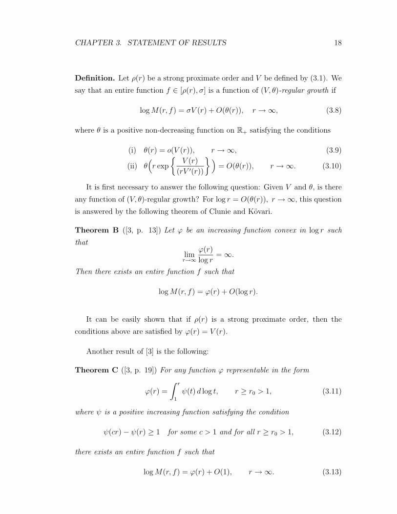
Definition. Let ρ(r) be a strong proximate order and V be defined by (3.1). We
say that an entire function f ∈ [ρ(r), σ] is a function of (V, θ)-regular growth if
log M(r, f) = σV (r) + O(θ(r)), r →∞, (3.8)
where θ is a positive non-decreasing function on R+ satisfying the conditions
(i) θ(r) = o(V (r)), r →∞, (3.9)
(ii) θ(r exp
V (r)
(rV ′(r))
)= O(θ(r)), r →∞. (3.10)
It is first necessary to answer the following question: Given V and θ, is there
any function of (V, θ)-regular growth? For log r = O(θ(r)), r →∞, this question
is answered by the following theorem of Clunie and Kovari.
Theorem B ([3, p. 13]) Let ϕ be an increasing function convex in log r such
that
limr→∞
ϕ(r)
log r= ∞.
Then there exists an entire function f such that
log M(r, f) = ϕ(r) + O(log r).
It can be easily shown that if ρ(r) is a strong proximate order, then the
conditions above are satisfied by ϕ(r) = V (r).
Another result of [3] is the following:
Theorem C ([3, p. 19]) For any function ϕ representable in the form
ϕ(r) =
∫ r
1
ψ(t) d log t, r ≥ r0 > 1, (3.11)
where ψ is a positive increasing function satisfying the condition
ψ(cr)− ψ(r) ≥ 1 for some c > 1 and for all r ≥ r0 > 1, (3.12)
there exists an entire function f such that
log M(r, f) = ϕ(r) + O(1), r →∞. (3.13)

CHAPTER 3. STATEMENT OF RESULTS 19
It is straightforward to show that if ρ(r) → ρ > 0 is a strong proximate
order, then conditions (3.11)-(3.12) are satisfied by ϕ(r) = V (r). Therefore, when
0 < ρ ≤ ∞, for each strong proximate order ρ(r) and for each θ satisfying (3.9)-
(3.10), there exists functions of (V, θ)-regular growth.
Our main result for functions of regular growth is the following:
Theorem 2 Let ρ(r) be a strong proximate order and let V be defined by (3.1).
If f is of (V, θ)-regular growth, then for all sufficiently large values of |w|, the
inequality
R(w, f)
|w| ≥ 1− exp
− C
|w|V ′(|w|)
√V (|w|)θ(|w|)
(3.14)
holds, where C is a positive constant.
The following corollary of Theorem 2 is immediate.
Corollary 1 If conditions of Theorem 2 are satisfied and, moreover,
lim infr→∞
rV ′(r)
√θ(r)
V (r)> 0, (3.15)
then
lim inf|w|→∞
R(w, f)V ′(|w|)√
θ(|w|)V (|w|) > 0. (3.16)
Examples.
1. Let f1(z) = sin z. Since log M(r, f1) = r + O(1) (see Example 2, page 5),
(3.16) implies (with V (r) = r, θ(r) = 1)
lim inf|w|→∞
R(w, f1)√|w| > 0.
One can compare this with Example 2, page 16.
2. Let V (r) = rρ(log r)m, 0 < ρ < ∞, m ∈ R. Assume log M(r, f) = V (r) +
O(1). Then (3.16) implies (with θ(r) = 1)
lim inf|w|→∞
R(w, f)
|w|√|w|ρ(log |w|)m > 0.

CHAPTER 3. STATEMENT OF RESULTS 20
3. Let V (r) = (log r)m, m > 1, and θ(r) = log r. Then (3.16) implies
lim inf|w|→∞
R(w, f)
|w|√
(log |w|)m−1 > 0.
4. Let V (r) = erm, m > 0, and θ(r) = 1. Then (3.16) implies
lim inf|w|→∞
R(w, f)
|w|√
e|w|m|w|m > 0.
Evidently, (3.16) gives a better estimate than (3.3). Moreover, the bound
(3.16) depends on θ and the smaller θ is, the better the bound is.
When 0 < ρ < ∞, using (3.7) we can put (3.16) into the form
lim inf|w|→∞
R(w, f)
|w|√
θ(|w|)V (|w|) > 0. (3.17)
If θ(r) = O(1), r → ∞, then the bound (3.17) is just Macintyre’s bound in
Theorem A (i) with limsup replaced by liminf and log M(|w|, f) replaced by
V (|w|). So, generally speaking, for functions of “very regular growth” Macintyre’s
bound is valid without any exceptional set.
We note that if ρ(r) is an admissible proximate order, then (3.15) holds for
θ ≡ 1 and hence for any non-decreasing positive θ. This is obvious when ρ = ∞.
When 0 < ρ < ∞, it follows immediately from (3.7). When ρ = 0, condition
(2.15) implies that eϑ/2 is convex and eϑ(xn)/2/xn → ∞ for some sequence xn →∞. This shows that (eϑ(x)/2)′ → ∞ as x → ∞. Since V (r) = eϑ(log r), it follows
thatrV ′(r)√
V (r)= 2r
(eϑ(log r)/2
)′ →∞, as r →∞.
Therefore Corollary 1 implies the following:
Corollary 2 Assume that f satisfies (2.14) and ρ(r) is an admissible proximate
order of f . If f is of (V, θ)-regular growth, then (3.16) holds.
We conjecture that (3.16) remains valid even for entire functions that do not
satisfy (2.14). The reason is that entire functions of very slow growth can not be
of “very regular growth” as the following theorem shows.

CHAPTER 3. STATEMENT OF RESULTS 21
Theorem D Let ρ(r) be a strong proximate order and let f be an entire function
satisfying
log M(r, f) = o(log2 r), r →∞. (3.18)
If f is of (V, θ)-regular growth, then
lim supr→∞
rV′(r)
√θ(r)
V (r)> 0. (3.19)
This theorem shows that the function θ in (3.8) has growth restrictions from
below. For example, if V (r) = logβ r, 1 < β < 2, then there is no entire function
f of (V, θ)-regular growth with θ(r) = o(log2−β r), r → ∞. In the next section
we will study this situation more deeply. We will not prove Theorem D since it
can be proved in much the same way as Theorem 4 below.
To consider the question whether the bound (3.16) is improvable or not, we
need examples of entire functions f for which
(a) | log M(r, f)− σV (r)| is relatively small,
(b) maximum modulus points of f are extremely close to its zero set.
For condition (a), we can use results of Clunie and Kovari [3] mentioned above.
Unfortunately, the method of these authors does not permit one to locate posi-
tions of zeros required for (b).
Nevertheless, we can prove that (3.16) is sharp if θ(r) is not of very slow
growth and has some special form, and if ρ(r) belongs to the class of strongly
admissible proximate orders.
Theorem 3 Let ρ(r) be a strongly admissible proximate order and let V be defined
by (3.1). Given 13≤ α < 1, put
θ(r) = V (r)(rV ′(r))α−1.
There exists an entire function f of (V, θ)-regular growth such that
lim inf|w|→∞
R(w, f)V ′(|w|)√
θ(|w|)V (|w|) ≤ π. (3.20)

CHAPTER 3. STATEMENT OF RESULTS 22
3.3 Growth irregularity of slowly growing entire
functions
Let A be the set of all increasing functions ϕ defined for r > 0, convex in log r,
and satisfying
limr→∞
ϕ(r)
log r= ∞. (3.21)
If f is a transcendental entire function, then the maximum modulus principle
and the Hadamard three circles theorem imply that log M(r, f) ∈ A. It is well
known that A is wider than the class of all functions of the form log M(r, f).
The following specific property of the latter can be mentioned: log M(r, f) must
be piecewise analytic (see, e.g., [19], p. 14, or [7], p. 11). The problem of the
asymptotic (at ∞) approximation of a function ϕ ∈ A by functions of the form
log M(r, f) can be viewed as the problem of existence of an entire function with
prescribed growth. From this point of view the problem has been studied by
Edrei and Fuchs [5], Clunie [2], and Clunie and Kovari [3]. Most complete results
are contained in [3] (see Theorem B and Theorem C, page 18 above.)
Recall that if the function ψ(r) := (d/d log r)ϕ(r) satisfies for some c > 1 the
condition
ψ(cr)− ψ(r) ≥ 1, r ≥ 1, (3.22)
then, by Theorem C, there exists an entire function f such that
log M(r, f)− ϕ(r) = O(1), r →∞. (3.23)
The restriction (3.22) implies that
lim infr→∞
ϕ(r)(log r)−2 > 0.
Therefore Theorem C is not applicable to functions ϕ ∈ A such that
ϕ(r) = o(log2 r), r →∞. (3.24)
Our aim in this section is to study this case. Our result concerns functions
that belong to a subset of A, which we describe now.

CHAPTER 3. STATEMENT OF RESULTS 23
Let us change the scale by setting log r = x. If f is a transcendental entire
function satisfying
log M(r, f) = o(log2 r), r →∞, (3.25)
then log M(ex, f) has growth (as a function of x) not less than of order 1 and
maximal type and not greater than of order 2 and minimal type. By Levin’s
theorem (see Section 2.3.), there exists a strong proximate order λ(x) of the form
λ(x) = λ +ϑ1(log x)− ϑ2(log x)
log x,
where 1 ≤ λ ≤ 2, ϑj ∈ C2(R+), j = 1, 2, is a concave function satisfying (2.12),
and
lim supx→∞
log M(ex, f)
xλ(x)= 1.
Moreover, as we have noted in Section 2.3, if f has maximal (minimal) type, then
one has ϑ2 ≡ 0 (ϑ1 ≡ 0).
Definition. We denote by B the set of all functions ϕ representable in the form
ϕ(ex) = w(x),
where w is defined by
w(x) := xλeϑ1(log x)−ϑ2(log x), (3.26)
1 ≤ λ ≤ 2, ϑ1 and ϑ2 have properties (2.12), and, moreover, if λ = 1, then ϑ2 ≡ 0,
if λ = 2, then ϑ1 ≡ 0.
The simplest examples of ϕ ∈ B are functions defined for sufficiently large r
in the form
ϕ(r) = (log r)p1(log2 r)p2 . . . (logm r)pm ,
where logk denotes the kth iteration of log, and p1, . . . , pm ∈ R are chosen in such
a way that (3.21) and (3.24) are satisfied.
Our main result of this section is the following:
CHAPTER 3. STATEMENT OF RESULTS 24
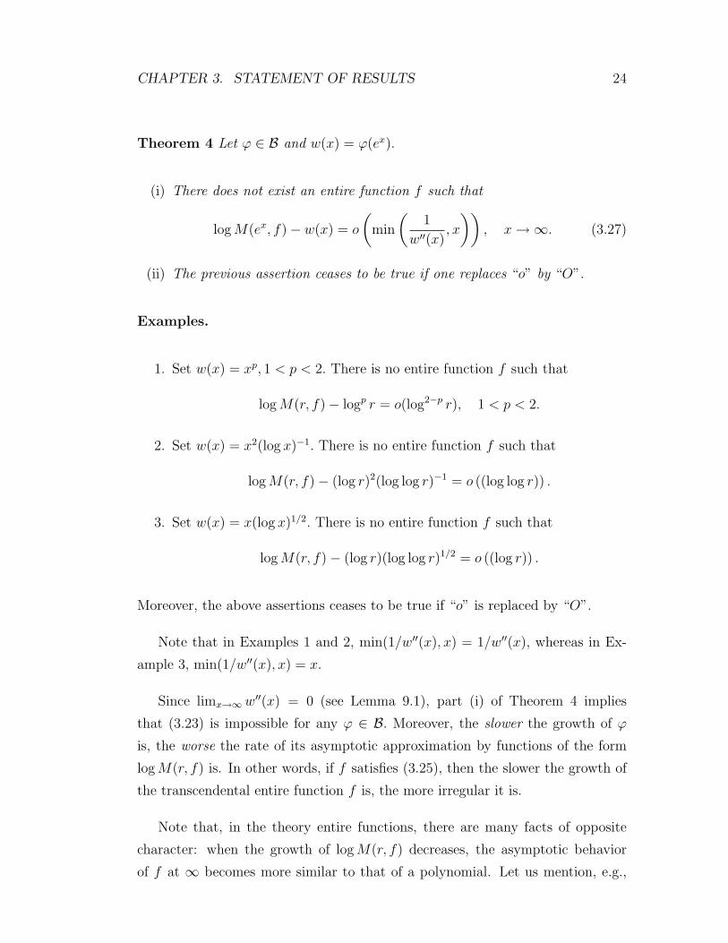
Theorem 4 Let ϕ ∈ B and w(x) = ϕ(ex).
(i) There does not exist an entire function f such that
log M(ex, f)− w(x) = o
(min
(1
w′′(x), x
)), x →∞. (3.27)
(ii) The previous assertion ceases to be true if one replaces “o” by “O”.
Examples.
1. Set w(x) = xp, 1 < p < 2. There is no entire function f such that
log M(r, f)− logp r = o(log2−p r), 1 < p < 2.
2. Set w(x) = x2(log x)−1. There is no entire function f such that
log M(r, f)− (log r)2(log log r)−1 = o ((log log r)) .
3. Set w(x) = x(log x)1/2. There is no entire function f such that
log M(r, f)− (log r)(log log r)1/2 = o ((log r)) .
Moreover, the above assertions ceases to be true if “o” is replaced by “O”.
Note that in Examples 1 and 2, min(1/w′′(x), x) = 1/w′′(x), whereas in Ex-
ample 3, min(1/w′′(x), x) = x.
Since limx→∞ w′′(x) = 0 (see Lemma 9.1), part (i) of Theorem 4 implies
that (3.23) is impossible for any ϕ ∈ B. Moreover, the slower the growth of ϕ
is, the worse the rate of its asymptotic approximation by functions of the form
log M(r, f) is. In other words, if f satisfies (3.25), then the slower the growth of
the transcendental entire function f is, the more irregular it is.
Note that, in the theory entire functions, there are many facts of opposite
character: when the growth of log M(r, f) decreases, the asymptotic behavior
of f at ∞ becomes more similar to that of a polynomial. Let us mention, e.g.,

CHAPTER 3. STATEMENT OF RESULTS 25
Wiman’s theorem on functions of order less than 1/2, theorems on functions of
order zero ([19], Sec.9, 15, 16, 26; [9]). Therefore, one might expect that, if the
growth of log M(r, f) diminishes, then its regularity increases. Theorem 4 shows
that this is not the case for entire functions satisfying (3.25).

Chapter 4
Preliminaries
Let f be an entire function of order ρ, 0 < ρ < ∞. It is proved by Levin [10, pp.
39–41] that f has its own strong proximate order. That is, there exists a strong
proximate order ρ(r) of the form (2.11) for which (2.8) holds. We have stated in
Section 2.3 that if the function f has maximal type with respect to the order ρ,
then one can choose ϑ2 ≡ 0. Correspondingly, if f has minimal type, then one
can choose ϑ1 ≡ 0. The first assertion easily follows from Levin’s construction
and we omit its proof. We will deduce the second assertion from the following
lemma.
Lemma 4.1 Let ϕ(x) be a non-positive continuous function on R+ such that
(i) limx→∞ ϕ(x) = −∞,
(ii) lim supx→∞ ϕ(x)/x = 0.
Then there exists a decreasing convex function ψ ∈ C2(R+) such that
(a) ψ(x) ≥ ϕ(x), ∀x > 0,
(b) ψ(x) = ϕ(x) on an unbounded set,
(c) limx→∞ ψ′′(x)/ψ′(x) = 0.
26

CHAPTER 4. PRELIMINARIES 27
Proof. Let l be the graph of ϕ :
l = (x, y) : y = ϕ(x), 0 < x < ∞.
We will construct ψ step by step.
Step 1. Consider the family of functions l1(t) : t > 0, where
l1(t) = (x, y) : y = y1(x, t) =1
x + 1− t, x > 0.
There exists a t1 > 0 such that the curve l1(t1) touches the curve l from above.
(This can be shown by using the arguments we apply in the proof of Lemma 4.3.)
The set of touching points is closed by continuity, and bounded by (i). Let x(1)1
be the abscissa of the last touching point. Take ε1 > 0 and choose x(2)1 > x
(1)1 + 1
so large that ∣∣∣∣∣y′′1(x
(2)1 , t1)
y′1(x(2)1 , t1)
∣∣∣∣∣ < ε1.
Consider the line tangent to l1(t1) at the point x(2)1 :
λ1 := (x, y) : y = y1(x) = y′1(x(2)1 , t1)(x− x
(2)1 ) + y1(x
(2)1 , t1), x ≥ x
(2)1 .
Note that by condition (ii), λ1 must intersect l.
λ1
x(1)2x
(0)2x
(2)1x
(1)1
ϕ
y1(x, t1)
y2(x, t2)

CHAPTER 4. PRELIMINARIES 28
Step 2. Consider the family l2(t), t ≥ 0, where
l2(t) = (x, y) : y = y2(x, t) = y1(x− t, t1) + y′1(x(2)1 , t1)t, x ≥ t.
Observe that l2(0) = l1(t1) and l2(t) is a shift of l1(t1) along the line λ1.
As before, there exists t2 > 0 such that l2(t2) lies above l and touches it along
a compact set. Let x(0)2 be the touching point of l2(t2) and λ1 and let x
(1)2 be
the abscissa of the last touching point of l2(t2) and l. Take ε2, 0 < ε2 < ε1, and
choose x(2)2 > x
(1)2 + 1 so large that
∣∣∣∣∣y′′2(x
(2)2 , t2)
y′2(x(2)2 , t2)
∣∣∣∣∣ < ε2.
Denote the line tangent to l2(t2) at the point x(2)2 by λ2:
λ2 := (x, y) : y = y2(x) = y′2(x(2)2 , t2)(x− x
(2)2 ) + y2(x
(2)2 , t2), x ≥ x
(2)2 .
We repeat this process indefinitely where the numbers ε1 > ε2 > ε3 > . . . are
chosen in such a way that εn ↓ 0.
With x(0)1 = 0, we set
ψ(x) =
yj(x, tj), x
(0)j ≤ x < x
(2)j ,
yj(x), x(2)j ≤ x < x
(0)j+1.
Then
ψ(x) ≥ ϕ(x) and ψ(x(1)j ) = ϕ(x
(1)j ).
Also∣∣∣∣ψ′′(x)
ψ′(x)
∣∣∣∣ < εj, x(0)j < x < x
(2)j ;
ψ′′(x)
ψ′(x)= 0, x
(2)j < x < x
(0)j+1.
Note that ψ′′ does not exist at the points x(0)j and x
(2)j but we can smooth ψ at
these points in such a way that all the properties (a)-(c) are preserved.
Lemma 4.2 Let f be an entire function of order ρ, 0 < ρ < ∞, and of minimal
type. Then f has a strong proximate order ρ(r) of the form (2.11) with ϑ1 ≡ 0.

CHAPTER 4. PRELIMINARIES 29
Proof. Let
θ(r) :=log M(r, f)
rρ.
Since f is of order ρ and minimal type, we have
lim supr→∞
log θ(r)
log r= 0 (4.1)
and
limr→∞
θ(r) = 0. (4.2)
Let ϕ(x) := log θ(ex). Then, because of (4.1) and (4.2), ϕ satisfies the hypothesis
of Lemma 4.1. Thus there exists a ψ satisfying (a)-(c) of Lemma 4.1. We set
ϑ2 ≡ −ψ. Using (a)-(b) we obtain
lim supr→∞
log M(r, f)
rρe−ϑ2(log r)= 1.
Therefore, ρ(r) = ρ− ϑ2(log r)/ log r is a strong proximate order of f .
If the order of an entire function is greater than 0, it is proved in [10] for
0 < ρ < ∞ and [4] for ρ = ∞ that f has its own strong proximate order.
It remains to show that any entire function f of order zero has a zero strong
proximate order.
We remind that a zero strong proximate order ρ(r) is a function representable
in the form ρ(r) = ϑ(log r)/ log r, where ϑ is a positive concave function satisfying
limx→∞
eϑ(x)
x= ∞; lim
x→∞ϑ(x)
x= 0; ϑ′′(x) + ϑ
′2(x) > 0, for x ≥ x0 > 0. (4.3)
Lemma 4.3 Every transcendental entire function f of order zero has a zero
strong proximate order.
Proof. We follow the idea of Levin’s proof [10, p. 39]. We write x = log r and
y = ϕ(x), where ϕ(x) = log log M(ex, f). Then ϕ is continuous and ϕ(x) → ∞as x →∞.
Since f is of order zero, we have
lim supx→∞
ϕ(x)
x= 0.
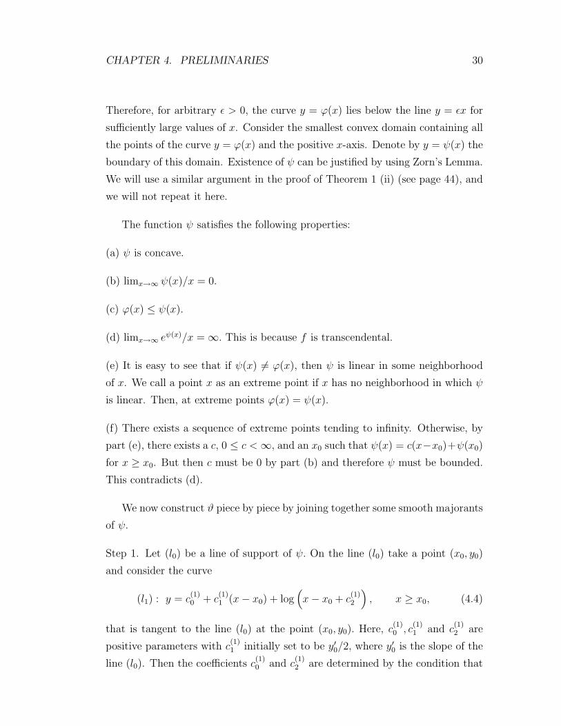
CHAPTER 4. PRELIMINARIES 30
Therefore, for arbitrary ε > 0, the curve y = ϕ(x) lies below the line y = εx for
sufficiently large values of x. Consider the smallest convex domain containing all
the points of the curve y = ϕ(x) and the positive x-axis. Denote by y = ψ(x) the
boundary of this domain. Existence of ψ can be justified by using Zorn’s Lemma.
We will use a similar argument in the proof of Theorem 1 (ii) (see page 44), and
we will not repeat it here.
The function ψ satisfies the following properties:
(a) ψ is concave.
(b) limx→∞ ψ(x)/x = 0.
(c) ϕ(x) ≤ ψ(x).
(d) limx→∞ eψ(x)/x = ∞. This is because f is transcendental.
(e) It is easy to see that if ψ(x) 6= ϕ(x), then ψ is linear in some neighborhood
of x. We call a point x as an extreme point if x has no neighborhood in which ψ
is linear. Then, at extreme points ϕ(x) = ψ(x).
(f) There exists a sequence of extreme points tending to infinity. Otherwise, by
part (e), there exists a c, 0 ≤ c < ∞, and an x0 such that ψ(x) = c(x−x0)+ψ(x0)
for x ≥ x0. But then c must be 0 by part (b) and therefore ψ must be bounded.
This contradicts (d).
We now construct ϑ piece by piece by joining together some smooth majorants
of ψ.
Step 1. Let (l0) be a line of support of ψ. On the line (l0) take a point (x0, y0)
and consider the curve
(l1) : y = c(1)0 + c
(1)1 (x− x0) + log
(x− x0 + c
(1)2
), x ≥ x0, (4.4)
that is tangent to the line (l0) at the point (x0, y0). Here, c(1)0 , c
(1)1 and c
(1)2 are
positive parameters with c(1)1 initially set to be y′0/2, where y′0 is the slope of the
line (l0). Then the coefficients c(1)0 and c
(1)2 are determined by the condition that
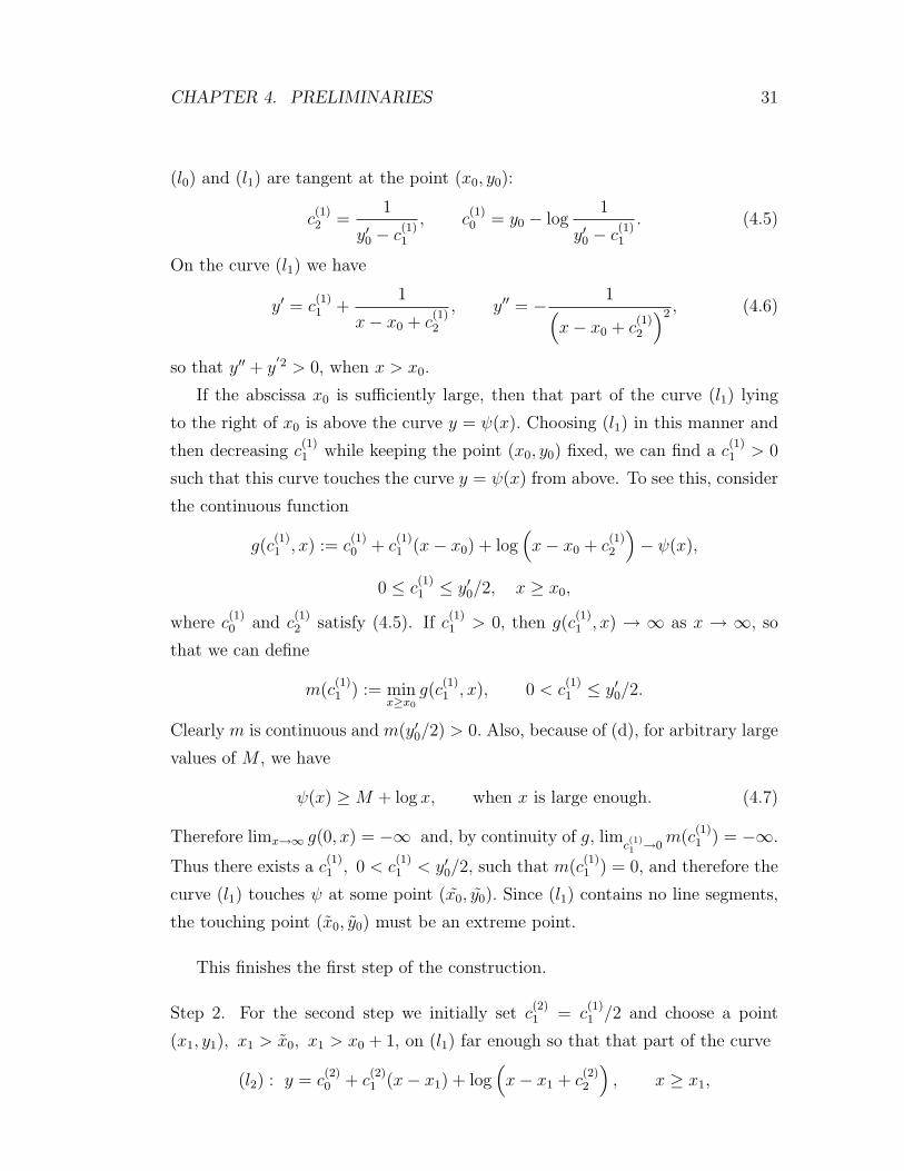
CHAPTER 4. PRELIMINARIES 31
(l0) and (l1) are tangent at the point (x0, y0):
c(1)2 =
1
y′0 − c(1)1
, c(1)0 = y0 − log
1
y′0 − c(1)1
. (4.5)
On the curve (l1) we have
y′ = c(1)1 +
1
x− x0 + c(1)2
, y′′ = − 1(x− x0 + c
(1)2
)2 , (4.6)
so that y′′ + y′2 > 0, when x > x0.
If the abscissa x0 is sufficiently large, then that part of the curve (l1) lying
to the right of x0 is above the curve y = ψ(x). Choosing (l1) in this manner and
then decreasing c(1)1 while keeping the point (x0, y0) fixed, we can find a c
(1)1 > 0
such that this curve touches the curve y = ψ(x) from above. To see this, consider
the continuous function
g(c(1)1 , x) := c
(1)0 + c
(1)1 (x− x0) + log
(x− x0 + c
(1)2
)− ψ(x),
0 ≤ c(1)1 ≤ y′0/2, x ≥ x0,
where c(1)0 and c
(1)2 satisfy (4.5). If c
(1)1 > 0, then g(c
(1)1 , x) → ∞ as x → ∞, so
that we can define
m(c(1)1 ) := min
x≥x0
g(c(1)1 , x), 0 < c
(1)1 ≤ y′0/2.
Clearly m is continuous and m(y′0/2) > 0. Also, because of (d), for arbitrary large
values of M , we have
ψ(x) ≥ M + log x, when x is large enough. (4.7)
Therefore limx→∞ g(0, x) = −∞ and, by continuity of g, limc(1)1 →0
m(c(1)1 ) = −∞.
Thus there exists a c(1)1 , 0 < c
(1)1 < y′0/2, such that m(c
(1)1 ) = 0, and therefore the
curve (l1) touches ψ at some point (x0, y0). Since (l1) contains no line segments,
the touching point (x0, y0) must be an extreme point.
This finishes the first step of the construction.
Step 2. For the second step we initially set c(2)1 = c
(1)1 /2 and choose a point
(x1, y1), x1 > x0, x1 > x0 + 1, on (l1) far enough so that that part of the curve
(l2) : y = c(2)0 + c
(2)1 (x− x1) + log
(x− x1 + c
(2)2
), x ≥ x1,

CHAPTER 4. PRELIMINARIES 32
(this curve is tangent to the curve (l1) at the point (x1, y1)), lying to the right
of this point, lies above the curve y = ψ(x). Then without changing the point
(x1, y1) we decrease c(2)1 so that (l2) touches the curve ψ. As in the first step we
have c(2)1 > 0.
Next we set c(3)1 = c
(2)1 /2 and take a point (x2, y2), x2 > x1 + 1, on (l2), and
form a curve (l3) etc.
Now we form ϑ from the segments of the curves (l0), (l1), . . . taken between
the points of contact, i.e. ϑ(x) = lj(x) when xj−1 ≤ x < xj, j ≥ 1 and ϑ(x) =
l0(x) when 0 < x < x0. Clearly, ϑ satisfies first two conditions of (4.3). Also
ϑ(x) ≥ ψ(x), with equality holding for a sequence of extreme points of ψ tending
to infinity. Using (c) and (e) we deduce that
lim supr→∞
log M(r, f)
eϑ(log r)= 1.
Evidently, ϑ(x) is twice continuously differentiable and satisfies the third condi-
tion of (4.3) except at the contact points xj. It is not difficult to see that we can
smooth ϑ in such a way that all the properties mentioned above are preserved.
This completes the proof of the lemma.
We noted in Section 2.4 that admissible proximate orders form a sufficient
class for characterization of the growth of entire functions that satisfy
lim supr→∞
log M(r, f)
log2 r= ∞. (4.8)
This is evident if the order of f is greater than zero, since for ρ > 0, any strong
proximate order is admissible. The following lemma shows that if f is of order
zero and satisfies (4.8), then there exists an admissible proximate order ρ(r) =
ϑ(log r)/ log r such that (2.15) and (2.8) holds.
Lemma 4.4 Every entire function f of order zero satisfying (4.8) has an admis-
sible proximate order.
Proof. The proof is similar to the proof of Lemma 4.3 with a few modifications
listed below. We change property (d) mentioned in the proof of Lemma 4.3 with

CHAPTER 4. PRELIMINARIES 33
(d’) lim supx→∞ eψ(x)/x2 = ∞.
We change (4.4) to
(l1) : y = c(1)0 + c
(1)1 (x− x0) + 2 log
(x− x0 + c
(1)2
), x ≥ x0,
so that 2ϑ′′(x) + ϑ′2(x) > 0. We change (4.7) to
ϑ(xn) ≥ M + 2 log xn, for some sequence xn.

Chapter 5
Auxiliary Results
In this chapter we will state and prove some auxiliary results that we will need
in the sequel.
5.1 Properties of proximate orders
Let ρ(r) be a proximate order. We will write
V (r) = rρ(r). (5.1)
It follows from the definitions in Section 2.2 that if ρ = 0 or ∞, then
V (r) = eϑ(log r), (5.2)
where, ϑ is a concave function that satisfies (2.9) if ρ = 0, and ϑ is a convex
function that satisfies (2.10) if ρ = ∞.
It is straightforward to check that in the case 0 < ρ < ∞,
rV ′(r) = (ρ + o(1))V (r). (5.3)
Lemma 5.1 ([10], Ch.1) Let ρ(r) be a proximate order such that ρ(r) → ρ,
0 ≤ ρ < ∞. Let V be defined by (5.1). Then
limr→∞
V (kr)
V (r)= kρ, (5.4)
34
CHAPTER 5. AUXILIARY RESULTS 35
uniformly an each interval 0 < a ≤ k ≤ b < ∞.
Proof. We have
logV (kr)
V (r)= [ρ(kr)− ρ(r)] log r + ρ(kr) log k.
Let us assume that 0 < a ≤ k ≤ 1. By Lagrange’s theorem, there exists some c
between kr and r such that
|ρ(kr)− ρ(r)| = (r − kr)|ρ′(c)|.
It is easy to check that (2.7) remains valid in the case ρ = 0. Therefore, for
arbitrary ε > 0 and for all sufficiently large values of r, we have
|ρ(kr)− ρ(r)| log r < εr − kr
kr log krlog r ≤ ε
(1
a− 1
)log r
log ar.
Hence
limr→∞
logV (kr)
V (r)= ρ log k
uniformly for 0 < a ≤ k ≤ 1.
The case k > 1 can be treated in a similar way.
We will now define a function ξ that we will use frequently. Let
ξ(r) := r exp
V (r)
rV ′(r)
, 0 ≤ ρ ≤ ∞. (5.5)
Then, by (5.2) and (5.3),
logξ(r)
r=
1
ϑ′(log r), ρ = 0 or ρ = ∞; (5.6)
logξ(r)
r=
1
ρ+ o(1), 0 < ρ < ∞. (5.7)
Evidently ξ(r) is greater than r. But it is not too much greater and we can
compare V (ξ(r)) and V (r):
Lemma 5.2 Let ξ be defined by (5.5). Then
lim supr→∞
V (ξ(r))
V (r)≤ e, 0 ≤ ρ ≤ ∞. (5.8)
CHAPTER 5. AUXILIARY RESULTS 36
Proof. We first deal with the case 0 < ρ < ∞. Since the convergence is uniform
in Lemma 5.1, it follows from (5.7) and (5.4) that the limit in (5.8) exists and
equals e.
When ρ = 0, using that ϑ in (5.2) is concave, we deduce
ϑ(log ξ(r))− ϑ(log r) = ϑ
(log r +
1
ϑ′(log r)
)− ϑ(log r) ≤ 1.
The proof for the case ρ = ∞ is longer. We first show that
limr→∞
ϑ′(log ξ(r))
ϑ′(log r)= 1, (ρ = ∞). (5.9)
To see this, observe that by the second condition in (2.10), for each ε > 0, there
exists an xε such that
1
y − x
(1
ϑ′(x)− 1
ϑ′(y)
)=
1
y − x
∫ y
x
ϑ′′(t)ϑ′2(t)
dt < ε, y > x > xε.
Letting y = log ξ(r), x = log r, we obtain
0 <1
log(ξ(r)/r)
ϑ′(log ξ(r))− ϑ′(log r)
ϑ′(log ξ(r))ϑ′(log r)
(5.6)=
ϑ′(log ξ(r))− ϑ′(log r)
ϑ′(log ξ(r))< ε, r > rε.
This implies (5.9).
To see (5.8), note that since ϑ is convex, we have
ϑ(log ξ(r))− ϑ(log r) ≤ log(ξ(r)/r)ϑ′(log ξ(r)) =ϑ′(log ξ(r))
ϑ′(log r).
Now (5.8) follows from this and (5.9).
The following corollary is immediate.
Corollary 5.3 Let ξ be defined by (5.5). Then
lim supr→∞
V (ξ(r))
rV ′(r) log(ξ(r)/r)≤ e. (5.10)
Lemma 5.4 Let C > 0 be a constant. Then
lim supr→∞
V ′(r + 1
CV ′(r)
)
V ′(r)≤ 1. (5.11)

CHAPTER 5. AUXILIARY RESULTS 37
Proof. For simplicity, let us write
R := r +1
CV ′(r). (5.12)
Consider first the case ρ = 0. We have
V ′(R)
V ′(r)=
ϑ′(log R)
ϑ′(log r)· V (R)
V (r)· r
R=: P1 · P2 · P3. (5.13)
Evidently P3 ≤ 1. Also, since ϑ is concave, P1 ≤ 1. To deal with P2, note that
0 ≤ ϑ(log R)− ϑ(log r) ≤ ϑ′(log r)(log R− log r) = ϑ′(log r) log
(1 +
1
CrV ′(r)
)
≤ ϑ′(log r)
CrV ′(r)=
ϑ′(log r)
Cϑ′(log r)V (r)=
1
CV (r)→ 0.
Therefore,
P2 =V (R)
V (r)= eϑ(log R)−ϑ(log r) → 1.
In the case 0 < ρ < ∞, note that rV ′(r) →∞ by (5.3). Then, it follows from
(5.3) and Lemma 5.1 that the limit exists in (5.11) and equals 1.
We will now deal with the case ρ = ∞. Let R,P1 − P3 be as in (5.12) and
(5.13). It is clear that rV ′(r) →∞. Therefore
P3 =r
R→ 1.
Since V (r) →∞,
ξ(r)− r = r
(exp
V (r)
rV ′(r)
− 1
)≥ r
V (r)
rV ′(r)=
V (r)
V ′(r)>
C
V ′(r)
for sufficiently large values of r. It follows that R < ξ(r) when r is large enough.
Hence, using (5.9) and monotonicity of ϑ′, we obtain
P1 =ϑ′(log R)
ϑ′(log r)→ 1. (5.14)
Finally, by the convexity of V and (5.14),
V (R)− V (r)
V (R)≤ V ′(R)(R− r)
V (R)=
ϑ′(log R)V (R)
RV (R)CV ′(r)=
1
C
ϑ′(log R)
ϑ′(log r)
r
R
1
V (r)→ 0.
It follows that P2 → 1 and the proof of the lemma is completed.
CHAPTER 5. AUXILIARY RESULTS 38
5.2 Properties of strong proximate orders
In this section ρ(r) will denote a strong proximate order. We continue to write
V (r) = rρ(r). (5.15)
In case ρ = 0 or ρ = ∞, we have
V (r) = eϑ(log r), (5.16)
where, ϑ is a concave function that satisfies (2.9) and (2.13) if ρ = 0 and ϑ is a
convex function satisfying (2.10) if ρ = ∞. When 0 < ρ < ∞, let us write
ϑ(x) = ϑ1(x)− ϑ2(x) + ρx, (0 < ρ < ∞),
where ϑ1 and ϑ2 are as in (2.11). Now (5.16) holds for all 0 ≤ ρ ≤ ∞. Note that,
by (2.12),
ϑ′(x) = ρ + o(1), (0 < ρ < ∞), (5.17)
ϑ′′(x) = o(1), (0 < ρ < ∞). (5.18)
We remind that a strong proximate order is also a proximate order. Therefore,
all the results proved in the previous section remain valid.
The following lemma will be useful for us.
Lemma 5.5 Let ρ(r) be a strong proximate order and V be defined by (5.15).
There exists a positive constant C not depending on r such that if∣∣∣∣logR
r
∣∣∣∣ ≤1
2
V (r)
rV ′(r), (5.19)
then
|V (R)− V (r)− log(R/r)rV ′(r)| ≤ C log2(R/r)(rV ′(r))2
V (r). (5.20)
Proof. Step 1. We first note that it suffices to show that there exist constants
C1, C2 and C3 such that
|ϑ(log R)− ϑ(log r)− log(R/r)ϑ′(log r)| ≤ C1 log2(R/r)ϑ′2(log r),(5.21)
|ϑ(log R)− ϑ(log r)| ≤ C2, (5.22)
|ϑ(log R)− ϑ(log r)| ≤ C3 |log(R/r)|ϑ′(log r). (5.23)

CHAPTER 5. AUXILIARY RESULTS 39
Indeed, if (5.22) and (5.23) holds, then for some constant C4,
∣∣eϑ(log R)−ϑ(log r) − 1− (ϑ(log R)− ϑ(log r))∣∣ ≤ C4 (ϑ(log R)− ϑ(log r))2
≤ C4C23 log2(R/r)ϑ′2(log r).
Combining this with (5.21) we obtain
∣∣eϑ(log R)−ϑ(log r) − 1− log(R/r)ϑ′(log r)∣∣ ≤ (C4C
23 + C1) log2(R/r)ϑ′2(log r).
This is equivalent to (5.20) since V (r) = eϑ(log r).
Step 2. We start with the case ρ = ∞. Assume first that r < R. To see
that (5.21) holds, observe that R < ξ(r) where ξ is defined in (5.5). Then, using
(2.10), (5.9) and monotonicity of ϑ′ we obtain
|ϑ(log R)− ϑ(log r)− log(R/r)ϑ′(log r)| =1
2log2(R/r)ϑ′′(c)
≤ log2(R/r)ϑ′2(log R)o(1)
≤ log2(R/r)ϑ′2(log r)o(1)
for some c between r and R. Further, it follows from the convexity of ϑ, (5.9) and
(5.19) that
|ϑ(log R)− ϑ(log r)| ≤ log(R/r)ϑ′(log R) = log(R/r)ϑ′(log r)(1 + o(1))
≤ 1
2+ o(1).
This shows (5.22) and (5.23).
Next we assume that r > R. By (2.10) and monotonicity of ϑ′,
|ϑ(log R)− ϑ(log r)− log(R/r)ϑ′(log r)| ≤ log2(R/r)ϑ′2(log r)o(1).
Further,
|ϑ(log R)− ϑ(log r)| ≤ log(r/R)ϑ′(log r)(5.19)
≤ 1
2.
Step 3. In the case 0 < ρ < ∞, reasoning as above and using (5.3), (5.17)
and (5.18), we easily obtain (5.21)-(5.23).

CHAPTER 5. AUXILIARY RESULTS 40
Step 4. We now deal with the case ρ = 0. Assume first that r < R. Note that
(2.13) implies
|ϑ′′(x)| < ϑ′2 (5.24)
when x is large enough. Therefore (for some c, r < c < R),
|ϑ(log R)− ϑ(log r)− log(R/r)ϑ′(log r)| =1
2log2(R/r)|ϑ′′(c)|
≤ 1
2log2(R/r)ϑ′2(log r).
Further, it follows from (5.19) and concavity of ϑ that
ϑ(log R)− ϑ(log r) ≤ log(R/r)ϑ′(log r) ≤ 1
2.
Hence (5.21)-(5.23) holds when r < R.
Assume now r > R. By (2.13), when x is sufficiently large, we have
0 ≤ −ϑ′′(x)
ϑ′2(x)< 1.
Hence1
ϑ′(y)− 1
ϑ′(x)=
∫ y
x
−ϑ′′(t)ϑ′2(t)
dt ≤ (y − x), y > x > x0.
Letting x = log R, y = log r and using (5.19), we obtain
1
ϑ′(log r)− 1
ϑ′(log R)≤ log
( r
R
)≤ 1
2
1
ϑ′(log r).
This implies
ϑ′(log R) ≤ 2ϑ′(log r). (5.25)
Using this and (5.24), we get
|ϑ(log R)− ϑ(log r)− log(R/r)ϑ′(log r)| ≤ 1
2log2(R/r)ϑ′2(log R)
≤ 2 log2(R/r)ϑ′2(log r).
Further, by the concavity of ϑ, (5.25) and (5.19),
|ϑ(log R)− ϑ(log r)| ≤ log(r/R)ϑ′(log R) ≤ 2 log(r/R)ϑ′(log r) ≤ 1.
This shows (5.22) and (5.23) and the proof of the lemma is completed.

Chapter 6
Proof of Theorem 1
By a well known theorem of Hadamard, log M(r, f) is a convex function of log r.
We define
K(r, f) :=d
d log rlog M(r, f) = r
d
drlog M(r, f). (6.1)
For definiteness, we take the right derivative in (6.1). Then K(r, f) is well defined
for all r > 0.
Note that, being the derivative of a convex function, K(r, f) is non-decreasing.
Note also that, since M(r, f) is strictly increasing, K(r, f) is non-negative. Esti-
mation of K(r, f) will play a fundamental role in the proofs of Theorems 1 and
2 (see Lemma 6.1 and 7.1).
Further, without loss of generality, we shall assume that f(0) = 1.
Lemma 6.1 Suppose that f ∈ [ρ(r), σ]. Then the following inequality holds:
lim supr→∞
K(r, f)
rV ′(r)≤ eσ. (6.2)
Proof. Since K(r, f) is non-negative and non-decreasing, for any R > r, we have
log M(R, f) =
∫ R
0
d
dtlog M(t, f) dt =
∫ R
0
K(t, f)
tdt ≥
∫ R
r
K(t, f)
tdt
≥ K(r, f)
∫ R
r
dt
t= K(r, f) log(R/r).
41

CHAPTER 6. PROOF OF THEOREM 1 42
We set R = ξ(r), where ξ is defined in (5.5). Then
lim supr→∞
K(r, f)
rV ′(r)≤ lim sup
r→∞
log M(R, f)
V (R)
V (R)
rV ′(r) log(R/r).
The desired result now follows from Corollary 5.3.
We will need the following corollary.
Corollary 6.2 We have
limr→∞
rV ′(r) = ∞.
Proof. Since f is transcendental, one has
limr→∞
K(r, f) = limr→∞
d log M(r, f)
d log r= ∞.
Therefore, the result follows from Lemma 6.1.
We will now prove part (i) of Theorem 1. Let w be a maximum modulus point
of f . We define
Φw(z) :=f(w + z)
f(w),
and
Q(h,w) := max|z|≤h
|Φw(z)|.
Since |f(w + z)| ≤ M(|w|+ |z|, f), we have
Q(h,w) ≤ M(|w|+ h, f)
M(|w|, f).
Therefore,
log Q(h,w) ≤ log M(|w|+ h, f)− log M(|w|, f) =
∫ |w|+h
|w|
d
dtlog M(t, f)dt
=
∫ |w|+h
|w|
K(t, f)
tdt ≤ K(|w|+ h, f)
∫ |w|+h
|w|
dt
t≤ K(|w|+ h, f)
h
|w| .
Using Lemma 6.1, we deduce that for each ε > 0, there exists rε such that
log Q(h,w) ≤ (eσ + ε)(|w|+ h)V ′(|w|+ h)h
|w| , |w| > rε. (6.3)

CHAPTER 6. PROOF OF THEOREM 1 43
We will now obtain a lower bound for R(w, f) in terms of Q(h,w). For this,
we define (see [12])
ηw(z) :=Q(Φw(z)− 1)
Q2 − Φw(z),
where Q = Q(h,w). Evidently, ηw(0) = 0 and |ηw(z)| ≤ 1 when |z| ≤ h. Applying
Schwarz’s Lemma we obtain
|ηw(z)| ≤ |z|h
, |z| ≤ h.
Hence,
Q|Φw(z)− 1| ≤ |z|h|Q2 − Φw(z)| ≤ |z|
h(|Q2 − 1|+ |Φw(z)− 1|).
This implies
|Φw(z)− 1| ≤ (|z|/h)(Q2 − 1)
Q− |z|/h , |z| ≤ h.
Since the right hand side is less than 1 when |z| < h/Q, it follows that Φw(z) 6= 0
and therefore f(w + z) 6= 0 for |z| < h/Q. This implies
R(w, f) ≥ h
Q. (6.4)
Combining (6.3) with (6.4) we deduce
R(w, f) ≥ h exp−(eσ + ε)(|w|+ h)V ′(|w|+ h)h
|w|, |w| > rε.
Setting
h =1
eσV ′(|w|) ,
we obtain
R(w, f)V ′(|w|) ≥ 1
eσexp
−(eσ + ε)
eσ
|w|+ h
|w|V ′(|w|+ h)
V ′(|w|)
, |w| > rε.
Note that by Corollary 6.2,
|w|+ h
|w| → 1 as |w| → ∞.
It follows, therefore, from Lemma 5.4 that
lim inf|w|→∞
R(w, f)V ′(|w|) ≥ 1
eσexp
−
(1 +
ε
eσ
).

CHAPTER 6. PROOF OF THEOREM 1 44
Since this is true for each ε > 0, the proof of Theorem 1.i is completed.
We proceed to prove part (ii) of Theorem 1. We denote by W (x) the greatest
convex minorant of V (ex). Existence of W can be deduced from Zorn’s Lemma.
Details are as follows:
Denote by F the set of all convex minorants of V (ex) on R+. F is not empty,
since if g(x) = 0,∀x ∈ R+, then g ∈ F . Let g1 ≤ g2 mean
g1(x) ≤ g2(x), ∀x ∈ R+.
Then ≤ defines a partial ordering on F . Pick any chain C ⊂ F . Let
h(x) := supg∈C
g(x), x ∈ R+.
The function h exists since at each point x ∈ R+, g(x) is bounded by V (ex).
Further, since each g ∈ C is convex, h is convex. Hence, h ∈ F and is an
upper bound of the chain C. Now, since each chain C ⊂ F has an upper bound,
Zorn’s Lemma asserts that the set F has a maximal element W. Next, let us
show that W is unique. If W1 and W2 are maximal elements of F , set W (x) :=
supW1(x),W2(x), x ∈ R+. Then Wi ≤ W, (i = 1, 2). But, by the maximality
of Wi, W ≤ Wi, (i = 1, 2). Therefore, W = W1 = W2.
Let us denote by H, the set of all touching points of W (x) and V (ex), i.e., let
H = x ∈ R+ : W (x) = V (ex).
Note that in the case ρ = ∞, V (ex) is convex, W (x) = V (ex) and H = R+.
One important property of H we will need is that it is unbounded. To see
this, first note thatV (ex)
x→∞ as x →∞. (6.5)
In the case 0 < ρ ≤ ∞, (6.5) clearly holds. When ρ = 0, it is the first of the
assumptions in (2.9). If a point x0 is not an element of H, i.e., if W (x0) < V (ex0),
then there exists a neighborhood of x0 in which W is linear. This can be easily
shown by using the fact that W (x) is the greatest convex minorant of V (ex). Now,

CHAPTER 6. PROOF OF THEOREM 1 45
suppose that H is bounded. Then, by the argument above, there exists x1 and
c, 0 ≤ c < ∞, such that for x ≥ x1,
W (x) = c(x− x1) + W (x1), x ≥ x1.
But, because of (6.5), this is impossible.
Evidently, W (x) is differentiable on H and W ′(x) = [V (ex)]′(x) for x ∈ H.
Moreover, W ′(x) →∞ as x →∞, x ∈ H.
We construct a sequence pn → ∞ in the following way: We set p1 = 1 and
choose pn, n ≥ 2, in such a way that the following conditions hold (recall the
definition of ξ(x) in (5.5)):
(i) log pn ∈ H (6.6)
(ii) pn > en−1pn−1 (6.7)
(iii) pn > ξ(pn−1) (6.8)
(iv) pnV′(pn) > n pn−1V
′(pn−1) (6.9)
(v)log r
V (r)<
1
n pn−1V ′(pn−1), when r > pn. (6.10)
It is possible to find such a sequence since H is unbounded, rV ′(r) → ∞ (by
Corollary 6.2) and log r/V (r) → 0 as r →∞ (by 6.5).
We set
f(z) =∞∏
k=1
(1 +
(z
pk
)[apkV ′(pk)] ),
where a is some positive constant to be determined later.
Let us first show that the following asymptotic equality holds:
log M(r, f) = [apnV ′(pn)] logr
pn
+ o(V (r)), as r →∞, pn ≤ r < pn+1.
(6.11)

CHAPTER 6. PROOF OF THEOREM 1 46
We have
log M(r, f) =∞∑
k=1
log(1 +
(r
pk
)[apkV ′(pk)] )
= [apnV ′(pn)] logr
pn
+n−1∑
k=1
[apkV′(pk)] log
r
pk
+
n∑
k=1
log(1 +
(pk
r
)[apkV ′(pk)] )+
∞∑
k=n+1
log(1 +
(r
pk
)[apkV ′(pk)] )
=: [apnV ′(pn)] logr
pn
+ S1 + S2 + S3.
We will show that
S1 = o(V (r)), S2 = O(1), S3 = O(1), r →∞, pn ≤ r < pn+1.
We start with S3. Since pk/pn+1 ≥ ek−1 for k ≥ n+2 (by 6.7) and pkV′(pk) →∞
(by Corollary 6.2), we find
S3 =∞∑
k=n+1
log(1 +
(r
pk
)[apkV ′(pk)] )≤ 1 +
∞∑
k=n+2
(pn+1
pk
)[apkV ′(pk)]
= O(1).
Similarly, since pn/pk ≥ ek for k ≤ n− 1, we obtain
S2 =n∑
k=1
log(1 +
(pk
r
)[apkV ′(pk)] )≤ 1 +
n−1∑
k=1
(pk
pn
)[apkV ′(pk)]
= O(1).
Finally,
S1 =n−1∑
k=1
[apkV′(pk)] log
r
pk
≤ a(log r)pn−1V′(pn−1)
n−1∑
k=1
pkV′(pk)
pn−1V ′(pn−1).
By condition (6.9), for k ≤ n− 2 we have
pkV′(pk)
pn−1V ′(pn−1)<
1
n− 1.
Therefore, using (6.10) we obtain
S1
V (r)≤ 2a
log r
V (r)pn−1V
′(pn−1) <2a
n.
Now, we will show that with an appropriate choice of a, f has type σ with
respect to ρ(r), i.e.,
σ = lim supr→∞
log M(r, f)
V (r).

CHAPTER 6. PROOF OF THEOREM 1 47
By (6.11) we have
lim supr→∞
log M(r, f)
V (r)= lim sup
r→∞r∈[pn,pn+1)
[apnV ′(pn)] log(r/pn) + o(V (r))
V (r)
= a lim supr→∞
r∈[pn,pn+1]
pnV ′(pn) log(r/pn)
V (r)
= a lim supn→∞
maxr∈[pn,pn+1)
pnV ′(pn) log(r/pn)
V (r)=: aσ.
Since, by condition (6.8), ξ(pn) ∈ [pn, pn+1), it follows from Corollary 5.3 that
σ ≥ lim supn→∞
pnV′(pn) log(ξ(pn)/pn)
V (ξ(pn))≥ e−1.
We proceed to find an upper bound for σ. We write x = log r, xn = log pn.
Then
σ = lim supn→∞
maxx∈[xn,xn+1)
[V (ex)]′(xn) · (x− xn)
V (ex).
Since xn = log pn belongs to H, we have [V (ex)]′(xn) = W ′(xn). Further, by the
definition of W , W (x) ≤ V (ex). Hence,
σ ≤ lim supn→∞
maxx∈[xn,xn+1)
W ′(xn)(x− xn)
W (x).
It now follows from the convexity of W that σ ≤ 1.
Now, setting a = σ/σ, we obtain that f ∈ [ρ(r), σ].
To complete the proof, it remains to show that f satisfies (3.4). Observe that
since f has non-negative Taylor coefficients, each pk ∈ R+ is a maximum modulus
point of f . Further, zeros of f are located at
pk exp
(iπ
1 + 2j
[apkV ′(pk)]
), j = 0, 1, . . . , [apkV
′(pk)]− 1.
Evidently,
R(pk, f) ≤∣∣∣∣pk − pk exp
(iπ
[apkV ′(pk)]
)∣∣∣∣ = 2pk sinπ
2[apkV ′(pk)].
Using Corollary 6.2, we deduce
lim infk→∞
R(pk, f)V ′(pk) ≤ π
a= π
σ
σ≤ π
σ.
This completes the proof of Theorem 1.

Chapter 7
Proof of Theorem 2
We start by proving the following amplification of Lemma 6.1 for functions of
(V, θ)-regular growth.
Lemma 7.1 If f is of (V, θ)-regular growth, then
K(r, f) = σrV ′(r) + O
(rV ′(r)
√θ(r)
V (r)
).
Proof. We set
logR
r:=
V (r)
rV ′(r)
√θ(r)
V (r).
By conditions (3.8)-(3.10), there exists a constant D such that
∣∣∣[log M(R, f)− log M(r, f)]− [σV (R)− σV (r)]∣∣∣ ≤ Dθ(r).
Further,
log M(R, f)− log M(r, f) =
∫ R
r
K(t, f)
tdt ≥ K(r, f) log
R
r.
We deduce
K(r, f) ≤ 1
log(R/r)[σV (R)− σV (r) + Dθ(r)].
48

CHAPTER 7. PROOF OF THEOREM 2 49
Note that because of (3.9), condition (5.19) is satisfied for sufficiently large values
of r. Application of Lemma 5.5 yields
K(r, f) ≤ 1
log(R/r)
(σ log(R/r)rV ′(r) + C log2(R/r)
[rV ′(r)]2
V (r)+ Dθ(r)
)
= σrV ′(r) + CrV ′(r)
√θ(r)
V (r)+ DrV ′(r)
√θ(r)
V (r).
For the reverse inequality we set
logr
s:=
V (r)
rV ′(r)
√θ(r)
V (r).
It follows from (3.8) and monotonicity of θ that, there exists a constant E such
that ∣∣∣[log M(r, f)− log M(s, f)]− [σV (r)− σV (s)]∣∣∣ ≤ Eθ(r).
Further,
log M(r, f)− log M(s, f) =
∫ r
s
K(t, f)
tdt ≤ K(r, f) log
r
s.
Hence,
K(r, f) ≥ 1
log(r/s)(σV (r)− σV (s)− Eθ(r)) .
Applying Lemma 5.5, we deduce that
K(r, f) ≥ 1
log(r/s)
(σ log(r/s)rV ′(r)− C log2(r/s)
[rV ′(r)]2
V (r)− Eθ(r)
)
= σrV ′(r)− CrV ′(r)
√θ(r)
V (r)− ErV ′(r)
√θ(r)
V (r).
This completes the proof of the lemma.
We will now prove Theorem 2. Let w be a maximum modulus point of f . We
define (see [12])
Ωw(z) :=f(wez)
f(w)e−K(|w|,f)z.
Let
P (h,w) := max|z|≤h
|Ωw(z)|.
CHAPTER 7. PROOF OF THEOREM 2 50
Setting |w| = r and Re z = t, we obtain
log P (h,w) ≤ max−h≤t≤h
(log M(ret, f)− log M(r, f)− tK(r, f)
).
We have
log M(ret, f)− log M(r, f)− tK(r, f) =
∫ ret
r
[K(u, f)−K(r, f)]du
u
=
∫ ret
r
[(K(u, f)− σuV ′(u))− (K(r, f)− σrV ′(r))]du
u+
+ σ
∫ ret
r
[uV ′(u)− rV ′(r)]du
u.
Application of Lemma 7.1 yields (for some constant C1)
log P (h,w) ≤ max−h≤t≤h
∣∣∣∫ ret
r
C1uV ′(u)
√θ(u)
V (u)
du
u
∣∣∣
+ max−h≤t≤h
∣∣∣∫ ret
r
C1rV′(r)
√θ(r)
V (r)
du
u
∣∣∣
+ σ max−h≤t≤h
∣∣∣V (ret)− V (r)− trV ′(r)∣∣∣
=: S1 + S2 + σS3.
We set
h = hr =V (r)
rV ′(r)1√
θ(r)V (r). (7.1)
Let us show that Si = O(1), i = 1, 2, 3.
By the monotonicity of θ and by condition (3.10), we have (for some constant
C2),
maxre−h≤u≤reh
θ(u) ≤ C2θ(r).
Therefore, (letting C3 = C1 · C2, C4 = 2 C3)
S1 ≤ C3
√θ(r) max
−h≤t≤h
∣∣∣∣∣∫ ret
r
V ′(u)√V (u)
du
∣∣∣∣∣ = C4
√θ(r) max
−h≤t≤h|√
V (ret)−√
V (r)|
= C4
√θ(r) max
−h≤t≤h
∣∣∣∣∣V (ret)− V (r)√V (ret) +
√V (r)
∣∣∣∣∣ ≤ C4
√θ(r)
V (r)max−h≤t≤h
|V (ret)− V (r)|

CHAPTER 7. PROOF OF THEOREM 2 51
We apply Lemma 5.5 and deduce that (for some constant C5)
S1 ≤ C4
√θ(r)
V (r)max−h≤t≤h
(|t|rV ′(r) + C5t
2 (rV ′(r))2
V (r)
)
≤ C4
√θ(r)
V (r)
(h rV ′(r) + C5h
2 (rV ′(r))2
V (r)
).
Inserting (7.1) into the above inequality we obtain
S1 ≤ C4 +C5√
θ(r)V (r).
Thus, S1 = O(1).
Clearly,
S2 = C1hrV ′(r)
√θ(r)
V (r)= C1.
Finally, application of Lemma 5.5 yields
S3 ≤ C6h2 (rV ′(r))2
V (r)=
C6
θ(r).
This implies S3 = O(1), since θ is nondecreasing.
We conclude that when h is as in (7.1),
P (h,w) = O(1), r = |w| → ∞. (7.2)
To prove the desired bound for R(w.f), we argue as we did in the proof of
Theorem 1. We write P := P (h,w) and define
ξw(z) =P (Ωw(z)− 1)
P 2 − Ωw(z).
Application of Schwarz’s Lemma shows that |ξw(z)| ≤ |z|/h for |z| ≤ h. This
implies
P |Ωw(z)− 1| ≤ |z|h|P 2 − Ωw(z)| ≤ |z|
h(P 2 − 1 + |Ωw(z)− 1|), |z| ≤ h.
We deduce
|Ωw(z)− 1| ≤ |z|/h(P 2 − 1)
P − |z|/h , |z| ≤ h. (7.3)

CHAPTER 7. PROOF OF THEOREM 2 52
Since, for |z| < h/P , right hand side of (7.3) is less than 1, we obtain
Ωw(z) 6= 0 for |z| < h
P.
Therefore,
f(wez) 6= 0 for |z| < h
P.
We conclude that
R(w, f) ≥ min|z|= h
P
|w − wez| = |w| min|z|= h
P
|1− ez| = |w|(
1− exp− h
P (h,w))
.
Inserting the value of h in (7.1) to the above inequality and using (7.2), we obtain
(3.14).

Chapter 8
Proof of Theorem 3
We will prove Theorem 3 for 0 < ρ < ∞. The cases ρ = 0 and ρ = ∞ can be
dealt in a similar way, therefore we will only outline their corresponding proofs.
We remind that for 0 < ρ < ∞, a strongly admissible proximate order is a
function ρ(r) ∈ C3(R+) representable in the form
ρ(r) = ρ +ϑ1(log r)− ϑ2(log r)
log r, r ≥ r0 > 1,
where ϑj (j = 1, 2), is a concave function of C3(R+) satisfying
(a) limx→∞
ϑj(x) = ∞, (8.1)
(b) limx→∞
ϑj(x)
x= 0, (8.2)
(c) limx→∞
ϑ′′j (x)
ϑ′j(x)= 0, (8.3)
(d) limx→∞
ϑ′′′j (x) = 0. (8.4)
With V (r) = rρ(r), a straightforward calculation shows that
rV ′(r) = (ρ + o(1))V (r), r →∞, (8.5)
r2V ′′(r) = (ρ2 − ρ + o(1))V (r), r →∞. (8.6)
Given 13≤ α < 1, we set
β :=1 + α
1− α. (8.7)
53
CHAPTER 8. PROOF OF THEOREM 3 54
Note that β ≥ 2. We define
νβ+1(r) := rV ′(r). (8.8)
It is easy to see that ν(r) is an increasing function when r is large enough.
By changing V (r) on a finite interval, we may assume that ν(r) increases for all
r > 0. Let
λ := ν−1 (8.9)
be the inverse function of ν. We set
f(z) :=∞∏
k=1
(1 +
(z
λ(k)
)[kβ ] ). (8.10)
(i) We first show that f satisfies (3.20). This is rather simple. Indeed, since
each point of the positive ray is a maximum modulus point, we have
R(λ(k), f) ≤ 2λ(k) sinπ
2[kβ].
Therefore,
lim infk→∞
kβ R(λ(k), f)
λ(k)≤ π.
Noting that
kβ+1 = (ν(λ(k)))β+1 = λ(k)V ′(λ(k)), (8.11)
we obtain the desired result.
(ii) Now we will prove that f is of (V, θ)-regular growth. This is much more
cumbersome.
Since f has nonnegative Taylor coefficients, we have
log M(r, f) =∞∑
k=1
log(1 +
(r
λ(k)
)[kβ ] )
=n∑
k=1
log( r
λ(k)
)[kβ ]
+n∑
k=1
log(1 +
(λ(k)
r
)[kβ ] )
+∞∑
k=n+1
log(1 +
(r
λ(k)
)[kβ ] )
=: S1 + S2 + S3, λ(n) ≤ r < λ(n + 1). (8.12)

CHAPTER 8. PROOF OF THEOREM 3 55
We will first show that S2 = O(1), S3 = O(1), r →∞. We begin with finding an
upper bound for (λ(k)/λ(k + 1))k.
Using (8.5) and (8.6) we obtain
ν ′(r) =ν(r)
r
(ρ
β + 1+ o(1)
). (8.13)
Since ν and λ are monotonic, we deduce
1 =
∫ λ(k+1)
λ(k)
ν ′(t)dt ≤ [λ(k + 1)− λ(k)]ν(λ(k + 1))
λ(k)
(ρ
β + 1+ o(1)
).
This implies,λ(k + 1)
λ(k)≥ 1 +
(β + 1)/ρ + o(1)
(k + 1).
Hence,
lim infk→∞
k logλ(k + 1)
λ(k)≥ β + 1
ρ. (8.14)
We choose C1 and C2 such that
C1 = C22 and e−
β+1ρ < C1 < C2 < 1.
Because of (8.14), there exists k0 such that
(λ(k)
λ(k + 1)
)k
< C1 when k > k0. (8.15)
Let n > k0. We have (recall that β ≥ 2)
S2 =n∑
k=1
log(1 +
(λ(k)
r
)[kβ ] )≤
n∑
k=1
(λ(k)
λ(n)
)k
= o(1) +n∑
k=k0+1
(λ(k)
λ(n)
)k
.
We divide the interval [k0+1, n] into two parts: Since λ(k) increases as k increases,
there exists n′ (depending on n) such that
λ(k)/λ(n) ≤ C2, k0 + 1 ≤ k ≤ n′
and
λ(k)/λ(n) ≥ C2, n′ < k ≤ n. (8.16)
CHAPTER 8. PROOF OF THEOREM 3 56
We have
S2 ≤ o(1) +n′∑
k=k0+1
(λ(k)
λ(n)
)k
+n∑
k=n′+1
(λ(k)
λ(n)
)k
=: o(1) + T1 + T2.
Evidently,
T1 ≤n′∑
k=k0+1
Ck2 ≤
∞∑
k=0
Ck2 .
We use backward induction to show that the following inequality holds:
(λ(k)
λ(n)
)k
≤ Cn−k2 , n′ + 1 ≤ k ≤ n− 1.
The base of induction (k = n− 1) holds because of (8.15). We assume
(λ(n− j)
λ(n)
)n−j
≤ Cj2 , j < n− (n′ + 1).
Since n − j > n′ + 1 we have, by (8.16), λ(n − j)/λ(n) ≥ C2. Using (8.15) we
obtain(
λ(n− j − 1)
λ(n)
)n−j−1
=
(λ(n− j − 1)
λ(n− j)
)n−j−1 (λ(n− j)
λ(n)
)n−jλ(n)
λ(n− j)
≤ C1.Cj2 .
1
C2
= Cj+12 .
Therefore,
T2 =n∑
k=n′+1
(λ(k)
λ(n)
)k
≤∞∑
k=0
Ck2 .
Thus S2 = O(1).
Using similar arguments it is easy to show that, when n > k0,
(λ(n + 1)
λ(k)
)k
≤ Ck−n−11 , k ≥ n + 2.
Hence,
S3 =∞∑
k=n+1
log(1 +
(r
λ(k)
)[kβ ] )≤
∞∑
k=n+1
(λ(n + 1)
λ(k)
)k
≤∞∑
k=0
Ck1 .
It remains to calculate the term S1 in (8.12). Our aim is to show that
S1 =V (r)
β + 1+ O (V α(r)) , r →∞, λ(n) ≤ r < λ(n + 1). (8.17)

CHAPTER 8. PROOF OF THEOREM 3 57
We write
S1 =n∑
k=1
[kβ] logr
λ(k)=
n∑
k=1
kβ logr
λ(k)−
n∑
k=1
(kβ − [kβ]) logr
λ(k)
=: U1 − U2.
We first deal with U1. Define
u1(t) := tβ logr
λ(t).
By Euler-Maclaurin sum formula, we have
U1 =n∑
k=1
u1(k) =
∫ n
1
u1(t)dt +1
2(u1(n) + u1(1)) +
1
12(u′1(n)− u′1(1))
−∫ n
1
u′′1(t)B2(t− [t])
2dt, (8.18)
where B2(t) is 2nd Bernoulli polynomial. We first evaluate∫ n
1u1(t)dt. We have
∫ n
1
u1(t)dt =nβ+1
β + 1log r −
∫ n
1
tβ log λ(t)dt + O(log r). (8.19)
Further, writing t = ν(s) and noting that ν and λ are inverse functions, we obtain
∫ n
1
tβ log λ(t)dt =
∫ λ(n)
λ(1)
νβ(s) log s dν(s)
=νβ+1(s) log s
β + 1
∣∣∣λ(n)
λ(1)− 1
β + 1
∫ λ(n)
λ(1)
νβ+1(s)
sds
(8.8)=
nβ+1 log λ(n)
β + 1− V (λ(n))
β + 1+ O(1). (8.20)
Combining (8.19) and (8.20) we find
∫ n
1
u1(t)dt =nβ+1
β + 1log
r
λ(n)+
V (r)
β + 1− 1
β + 1
(V (r)− V (λ(n))
)
+O(log r). (8.21)
We will need the following two properties (recall that λ(n) ≤ r < λ(n + 1)):
r
λ(n)− 1 = O(
1
n), n →∞, (8.22)
andV (r)
nβ+1→ 1
ρn →∞. (8.23)
CHAPTER 8. PROOF OF THEOREM 3 58
To see that (8.22) holds, note first that λ(n) ≤ r < λ(n + 1) implies n = [ν(r)].
Also, by (8.13),λ′(r)λ(r)
=1
r
(β + 1
ρ+ o(1)
). (8.24)
Therefore,
r − λ(n)
r=
1
r
∫ ν(r)
[ν(r)]
λ′(t)dt =1
r
∫ ν(r)
[ν(r)]
(β + 1
ρ+ o(1)
)λ(t)
tdt
≤ ((β + 1)/ρ + o(1)) r
nr= O(
1
n).
We have (8.23) since
nβ+1 = νβ+1(λ(n)) ≤ νβ+1(r) = V (r)(ρ + o(1)) ≤ νβ+1(λ(n + 1)) = (n + 1)β+1.
To estimate the term V (r) − V (λ(n)) that appeares in (8.21), note that by
(8.6), we have (for some c between λ(n) and r),
V (r)− V (λ(n))− (r − λ(n))V ′(λ(n)) =1
2
(r
λ(n)− 1
)2
λ2(n)V ′′(c)
(8.22)= O(
1
n2)O(V (r))
(8.23)= O (V α(r)) . (8.25)
Finally, combining (8.11), (8.21) and (8.25) we obtain∫ n
1
u1(t)dt =nβ+1
β + 1
[ (r
λ(n)− 1
)+ O
( (r
λ(n)− 1
)2 )]+
V (r)
β + 1
− 1
β + 1
[nβ+1
(r
λ(n)− 1
)+ O (V α(r))
]
=V (r)
β + 1+ O (V α(r)) . (8.26)
We now estimate the remaining terms that appear on the right hand side of
(8.18). It is easy to see that (8.2)-(8.4) implies
(log λ(t))(j) = O
(1
tj
), j = 1, 2. (8.27)
Therefore, for j = 1, 2, we have
u(j)1 (t) =
Γ(β + 1)
Γ(β − j + 1)tβ−j log
r
λ(t)−
j−1∑
l=0
(j
l
)(tβ)(l)(log λ(t))(j−l)
=Γ(β + 1)
Γ(β − j + 1)tβ−j log
r
λ(t)+ O(tβ−j). (8.28)

CHAPTER 8. PROOF OF THEOREM 3 59
Hence, using (8.22) we find
u(j)1 (n) = O(nβ−j−1) + O(nβ−j) = O(nβ−j), j = 1, 2. (8.29)
Also,
u1(n) = nβ logr
λ(n)= O(nβ−1). (8.30)
Finally, using (8.28) we find
∣∣∣∣∫ n
1
u′′1(t)B2(t− [t])
2dt
∣∣∣∣ ≤ D1
∫ n
1
tβ−2 logr
λ(t)dt + D2
∫ n
1
tβ−2dt
= D1tβ−1
β − 1log
r
λ(t)
∣∣∣n
1+
D1
β − 1
∫ n
1
tβ−1λ′(t)λ(t)
dt
+O(nβ−1)(8.24)= O(nβ−1) (8.31)
Thus, using (8.18), (8.26), (8.29), (8.30) and (8.31) we obtain
U1 =V (r)
β + 1+ O (V α(r)) .
Now we are going to estimate U2. Let
u2(t) := logr
λ(t).
Then
U2 ≤n∑
k=1
u2(k) =
∫ n
1
u2(t)dt +1
2(u2(n) + u2(1)) +
∫ n
1
u′2(t)γ(t)dt, (8.32)
where γ(t) = t− [t]− 1/2. We have
∫ n
1
u2(t)dt = t logr
λ(t)
∣∣∣n
1+
∫ n
1
tλ′(t)λ(t)
dt
(8.24)= n log
r
λ(n)+
∫ n
1
(β + 1
ρ+ o(1)
)dt + O(log r)
(8.22)= O(n). (8.33)
Thus, using (8.22), (8.27), (8.32) and (8.33) we obtain (recall that β ≥ 2)
U2 = O(n) = O(nβ−1) = O (V α(r)) .

CHAPTER 8. PROOF OF THEOREM 3 60
This shows (8.17) and the proof of Theorem 3, for the case 0 < ρ < ∞, is
completed.
When ρ = 0 or ρ = ∞ we define ν, λ and f as in (8.8)-(8.10). In the case
ρ = ∞ to prove that f is of (V, θ)-regular growth we first write a formula similar
to (8.12) and then show that
S1 =V (r)
β + 1+ O
( V α(r)
(ϑ′(log r))1−α
), S2 = O
( V α(r)
(ϑ′(log r))1−α
), S3 = O(1).
In the estimation of S1 we again use Euler-Maclaurin sum formula (8.18), but
now it is necessary to change (8.27) with
(log λ(t))(j) = O
(1
tj ϑ′(log λ(t))
), j = 1, 2, (8.34)
which follows from (2.10) and (2.17).
In the case ρ = 0 estimate (8.34) still holds because of (2.15) and (2.18).
Using this one can show that
S1 =V (r)
β + 1+ O
( V α(r)
(ϑ′(log r))1−α
), S2 = O(1), S3 = O(1).
Chapter 9
Proof of Theorem 4
The proof of Theorem 4 is based on a phenomenon discovered by Hayman [8] in
1966: for any transcendental entire function f , one has
lim supr→∞
(d
d log r
)2
log M(r, f) ≥ C0,
where C0 > 0 is an absolute constant. In 1974, Boichuk and Goldberg [1] proved
that, for functions f with non-negative Taylor coefficients, the best possible value
of C0 is 14. I.Ostrovskii found another proof based on a formula due to Rosenbloom
[17]. This proof has been included in [1]. We will use the idea of that proof for
getting a description of the set where
(d
d log r
)2
log M(r, f) ≥ ε2, 0 < ε <1
2.
The corresponding Lemma 9.5 below plays a crucial role in the proof of Theorem
4.
We begin by proving some lemmas.
Lemma 9.1 If ϕ ∈ B and w(x) = ϕ(ex), then
limx→∞
w′′(x) = 0.
61

CHAPTER 9. PROOF OF THEOREM 4 62
Proof. Since w has the form (3.26), we have
w′′(x) =w(x)
x2
(λ2 − λ + (2λ− 1)(ϑ1 − ϑ2)
′(log x)
+(ϑ1 − ϑ2)′2(log x) + (ϑ1 − ϑ2)
′′(log x)). (9.1)
Concavity of each ϑj, (j = 1, 2) and second condition of (2.12) imply that
ϑ′j(x) → 0, x →∞, (j = 1, 2). (9.2)
Using this and third condition of (2.12) we find
w′′(x) = xλ−2e(ϑ1−ϑ2)(log x)(
λ2 − λ + (2λ− 1)(ϑ1 − ϑ2)′(log x)
+o ((ϑ1 + ϑ2)′(log x))
). (9.3)
By the second condition of (2.12), for each α > 0, (ϑj(x)−αx) → −∞ as x →∞.
This implieseϑj(log x)
xα→ 0, x →∞ (α > 0). (9.4)
Now, for 1 ≤ λ < 2, the desired result follows from (9.2)-(9.4). For λ = 2, we
take into account that ϑ1 ≡ 0 and ϑ2 satisfies the first condition of (2.12).
Lemma 9.2 If ϕ ∈ B and w(x) = ϕ(ex), then
limx→∞
w′′(kx)
w′′(x)= kλ−2,
uniformly on each interval 0 < a ≤ k ≤ b < ∞.
Proof. By (9.3) we have
w′′(kx)
w′′(x)= kλ−2 exp (ϑ1 − ϑ2)(log kx)− (ϑ1 − ϑ2)(log x)
×λ2 − λ + (2λ− 1)(ϑ1 − ϑ2)′(log kx) + o ((ϑ1 + ϑ2)
′(log kx))
λ2 − λ + (2λ− 1)(ϑ1 − ϑ2)′(log x) + o ((ϑ1 + ϑ2)′(log x))
Using (2.12) (and, for λ = 1, that ϑ2 ≡ 0) we get the assertion of the lemma.
Lemma 9.3 If ϕ ∈ B and w(x) = ϕ(ex), then
limx→∞
(x− w(x)
w′(x)
)= ∞.

CHAPTER 9. PROOF OF THEOREM 4 63
Proof. From (3.26) it follows
x− w(x)
w′(x)=
(λ− 1)x + x(ϑ1 − ϑ2)′(log x)
λ + (ϑ1 − ϑ2)′(log x).
For λ > 1, assertion of the lemma follows from (9.2). For λ = 1, we take into
account that ϑ2 ≡ 0 and note that it suffices to show that limx→∞ xϑ′1(log x) = ∞or, equivalently,
limt→∞
etϑ′1(t) = ∞. (9.5)
By the third condition of (2.12), etϑ′1(t) is non-decreasing for sufficiently large
values of t. Therefore, if (9.5) does not hold, then ϑ′1(t) = O(e−t), t → ∞. This
contradicts the first condition of (2.12).
Lemma 9.4 It suffices to prove Theorem 4 under the additional assumption that
f has nonnegative Taylor coefficients.
Proof. We derive the lemma from the following theorem of Erdos and Kovari [6]:
Theorem. ([6]) Let f be an entire function. There exists an entire function f
with nonnegative Taylor coefficients such that
1
6≤ M(r, f)
M(r, f)≤ 3, r ≥ 0.
By this theorem, we have log M(r, f) = log M(r, f) + O(1). Therefore f
satisfies (3.27) (with “o” or “O”) if and only if so does f .
Let f be an entire transcendental function with nonnegative Taylor coeffi-
cients,
f(z) =∞∑
k=0
dkzk, dk ≥ 0, k = 0, 1, 2, . . . (9.6)
Then M(r, f) = f(r). We set
φ(x) = f(ex), α(x) = (log φ(x))′, β(x) = (log φ(x))
′′,
The function α(x) is nonnegative, increasing and tends to +∞ as x → +∞. Pick
ε ∈ (0, 1/2). The equations
α(ak) = k + ε, α(bk) = k + 1− ε, k = k0, k0 + 1, k0 + 2, . . . , (9.7)
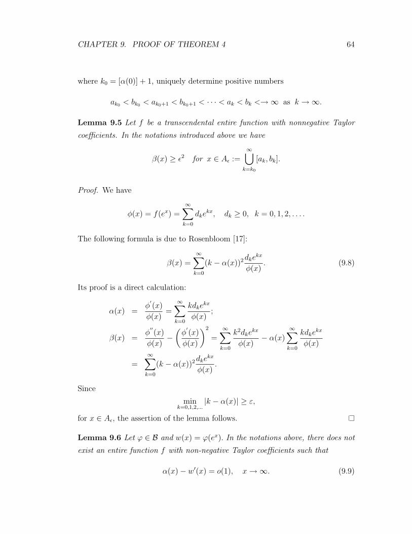
CHAPTER 9. PROOF OF THEOREM 4 64
where k0 = [α(0)] + 1, uniquely determine positive numbers
ak0 < bk0 < ak0+1 < bk0+1 < · · · < ak < bk <→∞ as k →∞.
Lemma 9.5 Let f be a transcendental entire function with nonnegative Taylor
coefficients. In the notations introduced above we have
β(x) ≥ ε2 for x ∈ Aε :=∞⋃
k=k0
[ak, bk].
Proof. We have
φ(x) = f(ex) =∞∑
k=0
dkekx, dk ≥ 0, k = 0, 1, 2, . . . .
The following formula is due to Rosenbloom [17]:
β(x) =∞∑
k=0
(k − α(x))2dkekx
φ(x). (9.8)
Its proof is a direct calculation:
α(x) =φ′(x)
φ(x)=
∞∑
k=0
kdkekx
φ(x);
β(x) =φ′′(x)
φ(x)−
(φ′(x)
φ(x)
)2
=∞∑
k=0
k2dkekx
φ(x)− α(x)
∞∑
k=0
kdkekx
φ(x)
=∞∑
k=0
(k − α(x))2dkekx
φ(x).
Since
mink=0,1,2,...
|k − α(x)| ≥ ε,
for x ∈ Aε, the assertion of the lemma follows.
Lemma 9.6 Let ϕ ∈ B and w(x) = ϕ(ex). In the notations above, there does not
exist an entire function f with non-negative Taylor coefficients such that
α(x)− w′(x) = o(1), x →∞. (9.9)

CHAPTER 9. PROOF OF THEOREM 4 65
Proof. Assume there exists such an entire function f . By (9.7) and (9.9) we have
1− 2ε = α(bk)− α(ak) = w′(bk)− w′(ak) + o(1) = w′′(ck)(bk − ak) + o(1),
for some ck ∈ (ak, bk). This implies (by Lemma 9.1),
(bk − ak) →∞ as k →∞.
On the other hand, by Lemma 9.1, there exists k1 such that
(α(x)− w′(x))′ = β(x)− w′′(x) ≥ ε2
2, x ∈ (ak, bk), k ≥ k1. (9.10)
This shows that the derivative of (α(x) − w′(x)) has a positive lower bound on
intervals of arbitrarily large length. This contradicts (9.9).
We will now prove part (i) of Theorem 4. In what follows, we agree to denote
by C positive constants.
We assume that there exists an entire function f with nonnegative Taylor
coefficients which satisfies (3.27). We will show that
α(x)− w′(x) = o(1), x →∞,
which contradicts Lemma 9.6.
We write
log φ(x)− w(x) =: τ(x),
where
|τ(x)| ≤ ε(x) min
(1
w′′(x), x
), ε(x) ↓ 0.
By Hadamard’s three circles theorem, log φ is convex. Therefore,
α(x)(z − x)− [log ϕ(z)− log ϕ(x)] ≤ 0, z > 0, x > 0.
Subtracting from both sides w′(x)(z − x)− [w(z)− w(x)], we obtain
[α(x)− w′(x)](z − x)− [(log ϕ(z)− w(z))− (log ϕ(x)− w(x))] ≤
≤ w(z)− w(x)− w′(x)(z − x) =1
2w′′(c)(z − x)2,
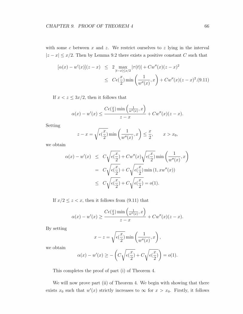
CHAPTER 9. PROOF OF THEOREM 4 66
with some c between x and z. We restrict ourselves to z lying in the interval
|z − x| ≤ x/2. Then by Lemma 9.2 there exists a positive constant C such that
[α(x)− w′(x)](z − x) ≤ 2 max|t−x|≤x/2
|τ(t)|+ Cw′′(x)(z − x)2
≤ Cε(x
2) min
(1
w′′(x), x
)+ Cw′′(x)(z − x)2.(9.11)
If x < z ≤ 3x/2, then it follows that
α(x)− w′(x) ≤Cε(x
2) min
(1
w′′(x), x
)
z − x+ Cw′′(x)(z − x).
Setting
z − x =
√ε(
x
2) min
(1
w′′(x), x
)≤ x
2, x > x0,
we obtain
α(x)− w′(x) ≤ C
√ε(
x
2) + Cw′′(x)
√ε(
x
2) min
(1
w′′(x), x
)
= C
√ε(
x
2) + C
√ε(
x
2) min (1, xw′′(x))
≤ C
√ε(
x
2) + C
√ε(
x
2) = o(1).
If x/2 ≤ z < x, then it follows from (9.11) that
α(x)− w′(x) ≥Cε(x
2) min
(1
w′′(x), x
)
z − x+ Cw′′(x)(z − x).
By setting
x− z =
√ε(
x
2) min
(1
w′′(x), x
),
we obtain
α(x)− w′(x) ≥ −(
C
√ε(
x
2) + C
√ε(
x
2)
)= o(1).
This completes the proof of part (i) of Theorem 4.
We will now prove part (ii) of Theorem 4. We begin with showing that there
exists x0 such that w′(x) strictly increases to ∞ for x > x0. Firstly, it follows

CHAPTER 9. PROOF OF THEOREM 4 67
from (9.3) that, w′′(x) > 0, for sufficiently large values of x (for λ = 1, we take
into account that ϑ2 ≡ 0 ). Further, direct calculation shows
w′(x) = xλ−1e(ϑ1−ϑ2)(log x)λ + (ϑ1 − ϑ2)′(log x).
Therefore, for 1 < λ ≤ 2, it follows from (9.2) and (9.4) that w′(x) → ∞. For
λ = 1, taking into account that ϑ2 ≡ 0, first condition of (2.12) yields w′(x) →∞.
We conclude that there exists unique xn →∞ such that
w′(xn) = n, n = n0, n0 + 1, . . . (9.12)
We define positive numbers cn, n ≥ n0, by the equation
log cn + nxn = w(xn). (9.13)
Since w(x) is strictly convex for x > xn0 , each of the lines
yn(x) := log cn + nx, n ≥ n0,
lies below the curve y = w(x) and is tangent to it at the point xn.
We set
f(z) =∞∑
n=n0
cnzn.
Sincelog cn
n= −xn +
w(xn)
w′(xn),
it follows from Lemma 9.3 that limn→∞ |cn|1/n = 0 and hence f is an entire
function.
We denote by µ(r, f) the maximum term of f . That is,
log µ(ex, f) = supn0≤n<∞
(log cn + nx).
The graph of log µ(ex, f) is a polygonal line lying below the graph of w(x) and
touching the latter only for x = xn. Thus, there exists a σn, xn < σn < xn+1, n ≥(n0 + 1), such that
log µ(ex, f) = log cn + nx, σn−1 ≤ x ≤ σn. (9.14)

CHAPTER 9. PROOF OF THEOREM 4 68
We shall prove the following:
w(x)− log µ(ex, f) = O
(min
(1
w′′(x), x
)), x →∞, (9.15)
log M(ex, f)− log µ(ex, f) = O(1), x →∞, (9.16)
from which Theorem 4 (ii) readily follows.
We will first show (9.15). Observe that log µ(ex, f) is differentiable on R+,
except at the points σn, n ≥ n0. For x > xn0 , we have
∣∣∣∣d
dx(w(x)− log µ(ex, f))
∣∣∣∣ ≤ 1, x 6= σn, n ≥ n0.
The integration from xn0 to x gives
0 ≤ w(x)− log µ(ex, f) ≤ x. (9.17)
Further, by Lemma 9.2, there exists a constant C∗ > 1 such that
1
C∗≤ w′′(x1)
w′′(x2)≤ C∗ for
1
e≤ x1
x2
≤ e, x1, x2 ≥ xn0 . (9.18)
Fix a constant D satisfying
D > max
(2C∗e,
1
2C3∗
). (9.19)
Assume now that (9.15) is not correct. Then, since (9.17) holds, there exists
y > exn0 such that
w(y)− log µ(ey, f) ≥ D
w′′(y). (9.20)
Using (9.17), we obtain w′′(y) ≥ D/y. Then
w′′(t) ≥ w′′(y)
C∗≥ D
C∗y≥ D
C∗et. (9.21)
for all t, y/e ≤ t ≤ ey.
Let n be such that xn ≤ y < xn+1. It follows from (9.21) and (9.19) that
w′(ey)− w′(y) =
∫ ey
y
w′′(t)dt ≥ D
C∗e> 2.

CHAPTER 9. PROOF OF THEOREM 4 69
This implies ey ≥ xn+2. Similarly, we find that w′(y)−w′(y/e) > 2 and therefore
y/e ≤ xn−1. Hence we have
y
e< σn−1 < xn < σn < xn+1 < σn+1 < ey.
There are two cases: Either xn ≤ y < σn or σn ≤ y < xn+1. If xn ≤ y < σn,
then by (9.13), (9.14) and (9.18),
w(y)− log µ(ey, f) = w(y)− log cn − ny
= w(y)− w(xn)− n(y − xn)
=1
2w′′(c)(y − xn)2 ≤ C∗
2w′′(y)(y − xn)2, (9.22)
where c ∈ (xn, σn). Moreover,
1 ≥ w′(y)− w′(xn) =
∫ y
xn
w′′(t)dt ≥∫ y
xn
w′′(y)
C∗dt = (y − xn)
w′′(y)
C∗. (9.23)
Combining (9.22) and (9.23), we find that
w(y)− log µ(ey, f) ≤ C3∗
2w′′(y). (9.24)
Similar reasoning shows that (9.24) also holds in the case σn ≤ y < xn+1. But
this contradicts (9.19) and (9.20).
It remains to show that (9.16) holds. Noting that w′′(x) → 0 (by Lemma
9.1) and w′(xn+1)− w′(xn) = 1 (by 9.12), we conclude that (xn+1 − xn) →∞ as
n →∞. Therefore, there exists an n1 ≥ n0 such that
xn+1 − xn ≥ 1, n ≥ n1.
Take any x ≥ xn1 . Let n be such that xn ≤ x < xn+1. Then, by (9.13), for
n1 ≤ k ≤ n− 1,
logcke
kx
cnenx= w(xk)− w(xn)− k(xk − xn) + (n− k)(xn − x)
≤ −∫ xn
xk
(w′(t)− k)dt ≤ −∫ xn
xk+1
(w′(t)− k)dt ≤ −∫ xn
xk+1
1 dt
≤ −(n− k − 1).

CHAPTER 9. PROOF OF THEOREM 4 70
Likewise, for k ≥ n + 2,
logcke
kx
cn+1e(n+1)x≤
∫ xk
xn+1
(w′(t)− k)dt ≤∫ xk−1
xn+1
(w′(t)− k)dt ≤∫ xk−1
xn+1
(−1) dt
≤ −(k − n− 2).
Thus, for xn ≤ x < xn+1,
M(ex, f) =∞∑
k=n0
ckekx
=
n1∑
k=n0
ckekx +
n−1∑
k=n1+1
ckekx + cnenx + cn+1e
(n+1)x +∞∑
k=n+2
ckekx
≤ µ(ex, f)
(n1∑
k=n0
ckekx
cnenx+
n−1∑
k=n1+1
ckekx
cnenx+ 2 +
∞∑
k=n+2
ckekx
cn+1e(n+1)x
)
≤ µ(ex, f)
(O(1) +
n−1∑
k=n1+1
e−(n−k−1) +∞∑
k=n+2
e−(k−n−2)
)
≤ Cµ(ex, f).
Hence, (9.16) holds and the proof of Theorem 4 is completed.

Bibliography
[1] V. S. Boichuk and A. A. Goldberg, On the three lines theorem, Mat. Zametki
15 (1974), 45–53.
[2] J. Clunie, On integral functions having prescribed asymptotic growth, Canad.
J. Math. 17 (1965), 396–404.
[3] J. Clunie and T. Kovari, On integral functions having prescribed asymptotic
growth, II, Canad. J. Math. 20 (1969), 7–20.
[4] J. P. Earl and W. K. Hayman, Smooth majorants for functions of arbitrarily
rapid growth, Math. Proc. Camb. Phil. Soc. 109 (1991), 565–569.
[5] A. Edrei and W. H. J. Fuchs, Entire and meromorphic functions with asymp-
totically prescribed characteristic, Canad. J. Math. 17 (1965), 383–395.
[6] P. Erdos and T. Kovari, On the maximum modulus of entire functions, Acta
Math. Acad. Sci. Hungar. 7 (1957), 305–312.
[7] A. A. Goldberg, B. Ya. Levin, and I. V. Ostrovskii, Entire and meromorphic
functions, Encyclopaedia of Math. Sci., vol. 85, 1996.
[8] W. K. Hayman, Note on Hadamard’s convexity theorem, Proc. Sympos. Pure
Math., La Jolla, Calif, 1966 (1968), 210–213.
[9] , The local growth of power series: a survey of the Wiman-Valiron
method, Canad. Math. Bull. 17 (1974), 317–358.
[10] B. Ya. Levin, Distribution of zeros of entire functions, revised ed., Transl.
Math. Monogr., vol. 5, Amer. Math. Soc., Providence, RI, 1980.
71

BIBLIOGRAPHY 72
[11] , Lectures on entire functions, Transl. Math. Monogr., vol. 150, Amer.
Math. Soc., Providence, RI, 1996.
[12] A. J. Macintyre, Wiman’s method and “flat regions” of integral functions,
Quart. J. Math. 9 (1938), 81–88.
[13] I. V. Ostrovskii and A. E. Ureyen, The growth irregularity of slowly growing
entire functions, Funct. Anal. Appl. (to appear).
[14] , Maximum modulus points and zero sets of entire functions of regular
growth, submitted.
[15] , Distance between a maximum modulus point and zero set of an entire
function, Complex Var. Theory Appl. 48 (2003), 583–598.
[16] , Maximum modulus points and zero sets of entire functions of regular
growth, C. R. Math. Acad. Sci. Paris 341 (2005), no. 8, 481–484.
[17] P. C. Rosenbloom, Probability and entire functions, in: Studies in mathe-
matical analysis and related topics (1962), 325–332.
[18] A. E. Ureyen, On maximum modulus points and the zero set for an entire
function of either zero or infinite order, Comput. Methods Funct. Theory 4
(2004), no. 2, 341–354.
[19] G. Valiron, Fonctions entieres d’ordre fini et fonctions meromorphes, Institut
de Mathematiques, Universite Geneve, 1960.