DISCUSSION PAPER SERIES

IZA DP No. 11839

Hector Sala

A Fresh Look at Fiscal Redistribution and Inequality in the US across Electoral Cycles

SEPTEMBER 2018

Any opinions expressed in this paper are those of the author(s) and not those of IZA. Research published in this series may include views on policy, but IZA takes no institutional policy positions. The IZA research network is committed to the IZA Guiding Principles of Research Integrity.The IZA Institute of Labor Economics is an independent economic research institute that conducts research in labor economics and offers evidence-based policy advice on labor market issues. Supported by the Deutsche Post Foundation, IZA runs the world’s largest network of economists, whose research aims to provide answers to the global labor market challenges of our time. Our key objective is to build bridges between academic research, policymakers and society.IZA Discussion Papers often represent preliminary work and are circulated to encourage discussion. Citation of such a paper should account for its provisional character. A revised version may be available directly from the author.

Schaumburg-Lippe-Straße 5–953113 Bonn, Germany

Phone: +49-228-3894-0Email: publications@iza.org www.iza.org

IZA – Institute of Labor Economics

DISCUSSION PAPER SERIES

IZA DP No. 11839

A Fresh Look at Fiscal Redistribution and Inequality in the US across Electoral Cycles

SEPTEMBER 2018

Hector SalaUniversitat Autònoma de Barcelona and IZA

ABSTRACT

IZA DP No. 11839 SEPTEMBER 2018

A Fresh Look at Fiscal Redistribution and Inequality in the US across Electoral Cycles*

The evolution of the ratio of direct taxation (characterized by progressive rates) over

indirect and payroll taxation (characterized by flat rates) is examined together with its

distributional consequences for the Bottom 50%, Middle 40% and Top 10% shares of

income. Oscillations of this ratio coincide with the US electoral cycles since the 1960s. We

show that periods in which this ratio increases coincide with those in which Democrats rule

the government and there is more redistribution from the rich (the Top 10%) to the rest of

the population. Conversely, periods in which this ratio falls and Republicans hold the power

are characterized by a fall in the ratio and less redistribution from the rich to the rest of the

population. Based on a set of counterfactual simulations, we hypothesize that the rich, as

informed economic agents, are able to protect themselves against tighter fiscal conditions,

thereby curtailing the redistributive effects of enhanced tax progressivity.

JEL Classification: H20, H31, E25

Keywords: electoral cycles, tax composition, income distribution, tax progressivity

Corresponding author:Hector SalaDepartament d’Economia AplicadaUniversitat Autónoma de Barcelona08193 BellaterraSpain

E-mail: hector.sala@uab.es

* I am grateful to the Spanish Ministry of Economy and Competitiveness for financial support through grant

ECO2016-75623-R.

2

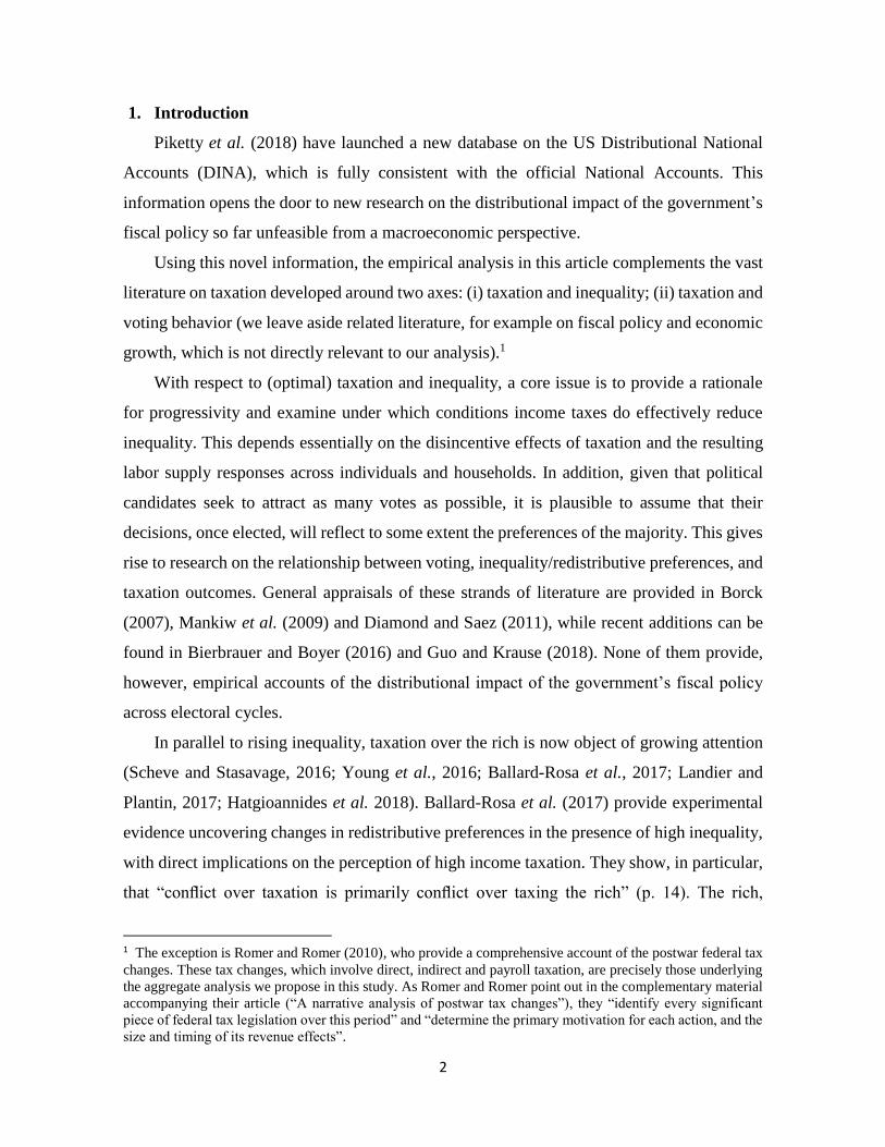
1. Introduction

Piketty et al. (2018) have launched a new database on the US Distributional National

Accounts (DINA), which is fully consistent with the official National Accounts. This

information opens the door to new research on the distributional impact of the government’s

fiscal policy so far unfeasible from a macroeconomic perspective.

Using this novel information, the empirical analysis in this article complements the vast

literature on taxation developed around two axes: (i) taxation and inequality; (ii) taxation and

voting behavior (we leave aside related literature, for example on fiscal policy and economic

growth, which is not directly relevant to our analysis).1

With respect to (optimal) taxation and inequality, a core issue is to provide a rationale

for progressivity and examine under which conditions income taxes do effectively reduce

inequality. This depends essentially on the disincentive effects of taxation and the resulting

labor supply responses across individuals and households. In addition, given that political

candidates seek to attract as many votes as possible, it is plausible to assume that their

decisions, once elected, will reflect to some extent the preferences of the majority. This gives

rise to research on the relationship between voting, inequality/redistributive preferences, and

taxation outcomes. General appraisals of these strands of literature are provided in Borck

(2007), Mankiw et al. (2009) and Diamond and Saez (2011), while recent additions can be

found in Bierbrauer and Boyer (2016) and Guo and Krause (2018). None of them provide,

however, empirical accounts of the distributional impact of the government’s fiscal policy

across electoral cycles.

In parallel to rising inequality, taxation over the rich is now object of growing attention

(Scheve and Stasavage, 2016; Young et al., 2016; Ballard-Rosa et al., 2017; Landier and

Plantin, 2017; Hatgioannides et al. 2018). Ballard-Rosa et al. (2017) provide experimental

evidence uncovering changes in redistributive preferences in the presence of high inequality,

with direct implications on the perception of high income taxation. They show, in particular,

that “conflict over taxation is primarily conflict over taxing the rich” (p. 14). The rich,

1 The exception is Romer and Romer (2010), who provide a comprehensive account of the postwar federal tax

changes. These tax changes, which involve direct, indirect and payroll taxation, are precisely those underlying

the aggregate analysis we propose in this study. As Romer and Romer point out in the complementary material

accompanying their article (“A narrative analysis of postwar tax changes”), they “identify every significant

piece of federal tax legislation over this period” and “determine the primary motivation for each action, and the

size and timing of its revenue effects”.

3

however, react to tighter fiscal conditions. Within the literature on optimal income taxation,

Landier and Plantin (2017) point to sophisticated tax plans and international tax arbitrage as

two channels by which affluent households respond to progressive taxation. Young et al.

(2016) exploit the information of 45 million of tax records to document millionaire tax flight

across US states. In this way, millionaire migration comes out as a third channel through

which affluent households deal with changes in tax progressivity. In the context of these

recent studies, which enhance our understanding of the elusive behavior of the rich vis-à-vis

taxation, we provide complementary evidence, by income share quantiles, on the effective

redistributive consequences of aggregate changes in fiscal progressivity.

More precisely, the purpose of this paper is to shed new light on the impact of tax

composition on income distribution across electoral cycles. By tax composition we point to

the ratio of total receipts from direct taxes over total receipts from (i) indirect taxes (taxes on

production and income) plus (ii) social security contributions (or payroll taxes). Income

distribution refers to the income shares commanded by the Bottom 50% (B50), the Middle

40% (M40), and the Top 10% (T10), which is the only structure of quantiles currently

allowed by the data (see Piketty et al., 2018). Finally, by electoral cycle we mean the periods

with the same political party holding the Federal government.

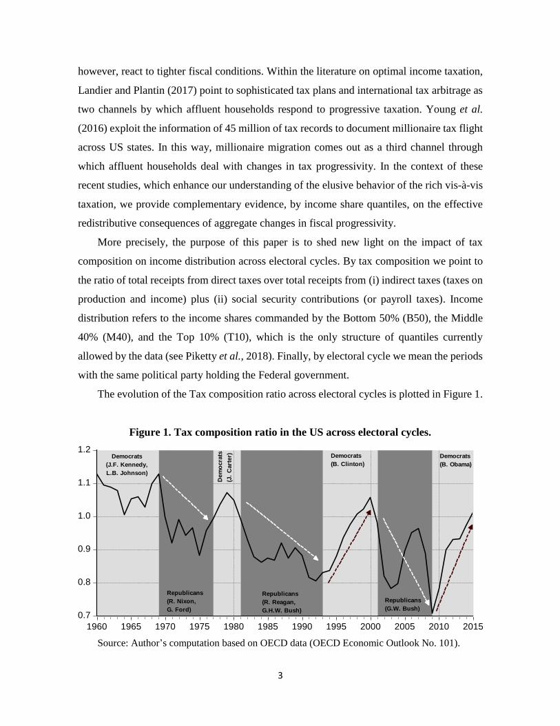
The evolution of the Tax composition ratio across electoral cycles is plotted in Figure 1.

Figure 1. Tax composition ratio in the US across electoral cycles.

0.7

0.8

0.9

1.0

1.1

1.2

1960 1965 1970 1975 1980 1985 1990 1995 2000 2005 2010 2015

Democrats

(B. Clinton)

Republicans

(R. Nixon,

G. Ford)

Dem

ocra

ts

(J.

Cart

er)Democrats

(J.F. Kennedy,

L.B. Johnson)

Republicans

(R. Reagan,

G.H.W. Bush)

Republicans

(G.W. Bush)

Democrats

(B. Obama)

Source: Author’s computation based on OECD data (OECD Economic Outlook No. 101).

4

We argue that the tax composition ratio depicted in Figure 1 can be considered a useful

proxy to track the aggregate evolution of the US tax system progressivity. First, because the

numerator contains a tax rate which grows with income and is thus progressive (Mankiw,

2010), while the two components in the denominator contain regressive taxes –i.e. they are

characterized by flat rates across income levels.2 Second, because the information contained

in this ratio is fully representative of the system as a whole –direct, indirect and payroll taxes

have accounted for 78%-87% of total government receipts between 1960 and 2016

(equivalent to 23%-29% of the US GDP).

Although such an aggregate appraisal cannot account for fiscal federalism issues

(taxation takes place also at a subnational levels), it is still a useful exercise to study the

extent to which the overall outcome of the US tax policy influences the widening gap between

the poor, the middle class and the rich. In addition, a potential caveat may arise from the

political orientation of the Congress, which differs frequently from the presidency (see Table

A1 in Appendix). As shown by Farrier (2010), however, the political orientation of the

Congress does not preclude the Federal government to implement its desired policies.3 The

comprehensive evidence she provides adds up to previous evidence by Sussman and Daynes

(1995) —according to which ideology is not the dominant factor in explaining the legislator’s

voting behavior—, and Lebo (2008) —showing that monthly congressional and presidential

approval data for the 1995-2005 period move in tandem, even during periods of divided

government.

Figure 1 is expressive in documenting a twofold pattern. First, a downward trend in

progressivity reflected in a 12% fall of the tax composition ratio between 1960 and 2016

(from 1.13 to 0.99). Second, a non-uniform downward path, highly sensitive to political

cycles, with recoveries under Democrat governments and relapses under Republican ones.

2 Payroll taxes are regressive. Piketty and Saez (2007) explain that the US payroll tax applies only up to a cap

and is therefore a relatively smaller tax burden as incomes rise above that cap. See Appendix 1 for more details. 3 The reason is an institutional ambivalence: “In the cycle of ambivalence, Congress forfeits its role in shaping

major policies to the president or some other entity that is not necessarily better prepared to see the national

interest, void of its own parochial interests or political motives. Members of Congress may hope that oversight

or legislative sunset give the institution a reserve of power to address problems that stem from delegation, but

it turns out that after-the-fact examination is much more complex than it appears, especially if the executive

branch is uncooperative or if vigorous and critical oversight does not make the leap into new law” (Farrier,

2010, p. 3).

5

Although this evolution is revealing, any particular value of this index should not be

considered as especially useful to assess the progressivity of the tax system in a given period.

For example, the fact that it takes a unit value in 2016 is not indicative of an aggregate

neutrality of the system in that year.

To define the progressivity of the system, we rather resort to the definition provided by

Piketty and Saez (2007), which is particularly appealing to our analysis: “(...) a more general

definition is that a tax system can be defined as progressive if after tax income is more equally

distributed than before tax income, and regressive if after tax income is less equally

distributed than before tax income” [Piketty and Saez (2007), p. 5]. It is an appealing

definition because under this light the data supplied by Piketty et al. (2018) becomes

particularly useful: it allows the distinction between the pre-tax and post-tax situation to be

applied to the income shares of the B50, M40 and T10 groups with information starting in

the 1960s. Hence, the fact that the pre-tax income share of the T10 has been systematically

above its post-tax counterpart (as reported in Table 3 below) yields to the conclusion that the

US tax system is progressive. This is along the lines of the analysis in Mankiw (2010).4

Piketty and Saez (2007) remark, however, that the progressivity of the system since the

1960s has moved in the direction of less progressivity along with the decline of the marginal

tax rates on the highest incomes; the reduction of corporate income taxes relative to corporate

profits (suggesting that capital owners –who are disproportionately of above-average

incomes– earn relatively more net of taxes today than in the 1960s, p. 3); and the substantial

increase in payroll tax rates. This fall is progressivity is confirmed by Hatgioannides et al.

(2018), who further document the rising fiscal inequality since the early 1960s by means of

a new Fiscal Inequality Coefficient.

In the context of a fiscal system gradually becoming less progressive, this article

provides a twofold contribution to the literature. First, we provide information, across

electoral cycles, on the global redistribution by income groups achieved through government

intervention in the US. Although it is well known that redistribution is a key element in left

wing ideology, to the best of our knowledge no quantitative assessment is yet available with

such an aggregate and temporal perspective. Second, we estimate how this redistribution

4 “It is simply wrong to say we don’t have a progressive tax system. The best analysis shows that average

federal tax rates rise steeply with income” [Mankiw (2010), p. 290].

6

reacts (across income groups) to a key determinant such as the tax composition ratio which,

as just argued, can be regarded as a useful aggregate time-series proxy of the falling trend

experienced by the progressivity of the US tax system. In doing so, we control for public

deficit and debt, so as to focus just on fiscal composition effects that modify the progressivity

ratio. We also control for GDP growth so that these composition effects can be assessed net

of business cycle oscillations.

Controlling for potential imbalances in public accounts allows us to exclude size effects

derived from expansionary or contractionary fiscal policies that would affect public deficit

and public debt. Our analysis, therefore, should be understood as complementary to the dense

strand of literature focusing on Keynesian and non-Keynesian effects of the fiscal policy and,

in the same vein, to studies that have dealt with the existence of electoral business cycles

where public expenditures tend to be the focus of the analysis. We also detach from the

presumption that party ideology is innocuous to tax progressivity. Along this line, four

different articles were invoked by Herwartz and Theilen (2017) to claim that party ideology

has no significant influence on the progressiveness of tax systems. Political parties, so the

argument goes, would have given up changes in the tax structure largely because of the

pressure brought by the globalization process; and would have progressively focused,

instead, on social spending policies to achieve welfare redistribution. Such behavior, in

addition, would help to explain why the literature connecting electoral and economic business

cycles has tended to focus on the expenditure side of government intervention.

Our findings refute party ideology neutrality and give credit to the alternative view: party

ideology matters and affects both fiscal progressivity and redistribution, which evolve along

electoral cycles. However, the enhanced progressivity and resulting expected redistribution

from the rich to the poor when Democrats hold the power, does not fully counterbalance the

lack of redistribution and increased inequality under Republican governments. Moreover,

when Democrats govern there is a distributional loss that can be associated to the riches’

reaction to cover themselves against tighter fiscal conditions.

The remainder of this paper is structured as follows. Section 2 defines the variables used

and presents the estimated models. Section 3 makes use of these models to conduct dynamic

simulations and asses the incidence of tax composition on income distribution. Section 4

concludes.

7

2. Data and estimation

2.1. Variables

Data on post-tax and pre-tax income shares for the B50, M40 and T10 groups is obtained

from Piketty et al. (2018). To evaluate how redistributive public action is we subtract these

series from one another so as to have a measure of how government intervention affects each

of the groups. This is done in the spirit of Solt (2016), who defines the concept of absolute

redistribution as the difference between market income inequality (pre-tax, pre-transfer) and

net income inequality (post-tax, post-transfer), where income inequality is measured by the

Gini coefficient.

In our case, given that taxes and transfers have a different impact across groups, we

distinguish different measures of redistribution. Two measures of positive redistribution

(𝑃_𝑅𝐸𝐷𝐵50 and 𝑃_𝑅𝐸𝐷𝑀40) are defined as the post-tax income share of, respectively, the

B50 and M40 groups, minus the corresponding pre-tax income shares.5 Then, a measure of

negative redistribution (𝑁_𝑅𝐸𝐷𝑇10) is defined as the pre-tax income share of the T10 minus

the corresponding post-tax income share. These two ways of defining redistribution will be

useful in the interpretation of the empirical analysis.

Data on tax revenues from direct, indirect and payroll taxation (denoted respectively as

(𝐷𝑇, 𝐼𝑇 and 𝑃𝑇) is obtained from the OECD Economic Outlook and used to compute the

tax composition ratio (𝑇𝐶𝑅) as 𝑇𝐶𝑅 = 𝐷𝑇/(𝐼𝑇 + 𝑃𝑇). We also gather information on public

deficit (𝑃_𝐷𝐸𝐹), defined as government net lending; public debt (𝑃_𝐷𝐸𝐵𝑇), defined as

general government net financial liabilities; and Gross Domestic Product (𝐺𝐷𝑃).

Data availability for the variables supplied by Piketty et al. (2018) runs from 1962 to

2014. Those from the OECD Economic Outlook run from 1960 to 2016. Given the dynamic

nature of the estimated models and the inclusion of instruments the effective sample period

becomes 1964-2014.

5 Post-tax here is along the lines of Piketty et al. (2018). It refers to the situation once the public sector has

undertaken all its redistributive action through taxes (all taxes) and spending (all included: cash transfers, in-

kind transfers and collective consumption expenditures).

8

2.2. Models

Provided with these variables, the empirical specifications to be estimated are:

𝑃_𝑅𝐸𝐷𝑡𝐵50 = 𝑐𝑡 + ∑ 𝛼𝑗𝑃_𝑅𝐸𝐷𝑡−𝑗

𝐵50

𝐽

𝑗=1

+ ∑ 𝛽𝑗𝑇𝐶𝑅𝑡−𝑗

𝐽

𝑗=1

+ ∑ 𝛾𝑗

𝑃_𝐷𝐸𝐹𝑡−𝑗

𝐺𝐷𝑃𝑡−𝑗

𝐽

𝑗=0

+ ∑ 𝛿𝑗

𝑃_𝐷𝐸𝐵𝑇𝑡−𝑗

𝐺𝐷𝑃𝑡−𝑗

𝐽

𝑗=0

+ ∑ 𝜆𝑗Δ𝐺𝐷𝑃𝑡−𝑗

𝐽

𝑗=0

+ 휀𝑡 (1)

𝑃_𝑅𝐸𝐷𝑡𝑀40 = 𝑐𝑡

′ + ∑ 𝛼𝑗′𝑃_𝑅𝐸𝐷𝑡−𝑗

𝑀40

𝐽

𝑗=1

+ ∑ 𝛽𝑗′𝑇𝐶𝑅𝑡−𝑗

𝐽

𝑗=1

+ ∑ 𝛾𝑗′

𝑃_𝐷𝐸𝐹𝑡−𝑗

𝐺𝐷𝑃𝑡−𝑗

𝐽

𝑗=0

+ ∑ 𝛿𝑗′

𝑃_𝐷𝐸𝐵𝑇𝑡−𝑗

𝐺𝐷𝑃𝑡−𝑗

𝐽

𝑗=0

+ ∑ 𝜆𝑗′Δ𝐺𝐷𝑃𝑡−𝑗

𝐽

𝑗=0

+ 휀𝑡′ (2)

𝑁_𝑅𝐸𝐷𝑡𝑇10 = 𝑐𝑡

′′ + ∑ 𝛼𝑗′′𝑃_𝑅𝐸𝐷𝑡−𝑗

𝑇10

𝐽

𝑗=1

+ ∑ 𝛽𝑗′′𝑇𝐶𝑅𝑡−𝑗

𝐽

𝑗=1

+ ∑ 𝛾𝑗′′

𝑃_𝐷𝐸𝐹𝑡−𝑗

𝐺𝐷𝑃𝑡−𝑗

𝐽

𝑗=0

+ ∑ 𝛿𝑗′′

𝑃_𝐷𝐸𝐵𝑇𝑡−𝑗

𝐺𝐷𝑃𝑡−𝑗

𝐽

𝑗=0

+ ∑ 𝜆𝑗′′Δ𝐺𝐷𝑃𝑡−𝑗

𝐽

𝑗=0

+ 휀𝑡′′ (3)

where 𝑡 denotes time and 𝑗 denotes lags; 𝑐 is the constant; the α’s, 𝛽’s, 𝛾’s, 𝛿’s and 𝜆’s

are parameters to be estimated; ∆ is the difference operator; and 휀 is the error term.

Amid the scarce literature empirically connecting redistribution (not inequality) and

public policies in a macroeconomic setting, models (1) to (3) resemble those estimated in

Battisti and Ziera (2016) in which redistribution is explained by a set of fiscal policy

variables. The difference is that Battisti and Ziera (2016) use cross-section and panel data for

a wide set of countries, while we focus on a time series analysis.

The estimation process is conducted following the AutoRegressive Distributed Lag

9

(ARDL) or Bounds Testing Approach (Pesaran and Shin, 1999; and Pesaran et al., 2001).

The best functional form is selected according to the standard selection criteria (Akaike,

Schwarz) among those specifications that meet the standard misspecification tests (of

residual autocorrelation, normality, heteroscedasticity and linearity) and structural stability

tests (cusum and cusum2). Such specifications are first estimated by Ordinary Least Squares

(OLS). Then, to take into account potential endogeneity and check for the robustness of the

estimated economic relationships, we also conduct estimations by the General Method of

Moments (GMM) and Two Stages Least Squares (2SLS).

Regarding endogeneity, note that progressivity enters with a lag in all three equations.

This is consistent with the lag at which tax payments take place and helps to deal with the

potential endogeneity of this crucial variable. In addition, economic growth is considered as

endogenous to take into account that it reacts to the fiscal policy. Accordingly, given the

time-series nature of our analysis, the selected instruments consist of two lags of the

dependent variable, and up to three lags of the explanatory variables progressivity and

economic growth (three lags of GDP are included in equation (3) where the second lag

enters as explanatory variable).

Our main parameter of interest is 𝛽, which captures the short-run influence of the tax

composition ratio on redistribution for the B50, M40 and T10 groups. In turn, the

corresponding long-run impact (for the B50 group) is given by ∑ 𝛽𝑗𝑇𝐶𝑅𝑡−𝑗

𝐽𝑗=0

1−∑ 𝛼𝑗𝑃_𝑅𝐸𝐷𝑡−𝑗𝐵50𝐽

𝑗=1

. The

expected outcome is a positive coefficient indicating that, ceteris paribus, the larger the

aggregate tax progressivity is (as proxied by the tax composition ratio), the more

redistribution is achieved. Note that such redistribution is positive for the B50 and M40

groups (as their situation post-tax is better off), while it is negative for the T10 (since they

are net contributors to the system). Hence, given the way we have defined redistribution for

these three groups, we expect a positive coefficient of 𝛽 in the three estimated models (this

clean expected output justifies the way we have defined the redistribution affecting the

different groups).

The ceteris paribus assumption is granted by three control variables whose influence is

captured by the estimated parameters 𝛾, 𝛿 and 𝜆. The first two fix the situation of public

accounts and allow the estimate of 𝛽 to capture solely tax composition effects at a given

10

level of (i) public revenues or expenditures –hence the control by public deficit–; and (ii) net

financial liabilities –hence the control by public debt. Estimation of the short and long-run

impacts of 𝛾 and 𝛿 provide, as a by-product, information on size effects –i.e. on the

influence, on each group, of budget deviations (via lower tax revenues, higher public

expenditures, or indebtedness) on redistribution for a given tax composition ratio.

Economic growth aims at controlling for business cycle oscillations, given that being in

a rise or a in a slump conditions the instruments used to conduct the economic policy. As an

example, think on the automatic stabilizers which are precisely designed to offset business

cycle fluctuations. It is to control for compositional changes in public intervention driven by

such oscillations that we also include economic growth. As a by-product, the estimation of

𝜆 and its long run impact by group provides valuable information on the segment of

population that benefits the most from economic growth.

2.3. Estimates

Table 1 presents the estimated results for equations (1), (2) and (3).

The coefficient on the tax composition ratio is positive and significant for the B90 and

the M40 groups. This implies that increases in the proportion of tax revenues obtained from

direct taxation (relative to those obtained from indirect taxation and social security

contributions) contribute to increase redistribution (the gap between their post-tax and pre-

tax income shares widens). The estimated coefficient is also positive for the Top 10%,

indicating that further progressivity increases redistribution also for the rich. However, this

redistribution is negative in the sense that it erodes the post-tax income shares of the rich

relative to their pre-tax situation.

Another important observation is the lower long-run sensitivity of the B50 group to the

tax composition ratio (with a long-run coefficient amounting to 0.08) relative to the one of

the M40 and T10 groups (which is twice as large when taking as reference the GMM and

2SLS estimates). Given that redistribution only hurts the T10 income shares, we have

conducted complementary regressions within this group to check whether we can identify

different behaviors at different levels of income. The resulting estimations confirm positive

coefficients, but with decreasing statistical significance. This coefficient is still significant

for the Top 5% and Top 1% groups (at 5% and 6% critical values), but it ceases to be

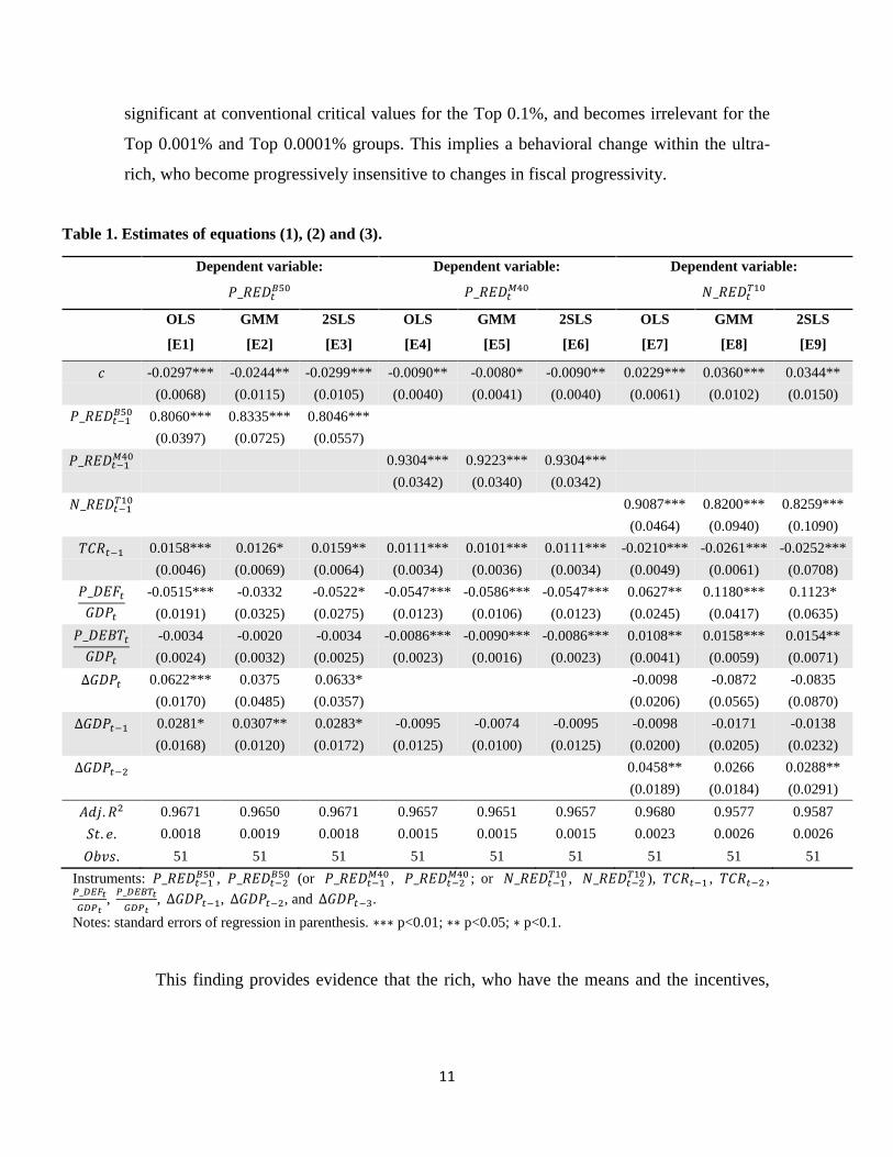
11

significant at conventional critical values for the Top 0.1%, and becomes irrelevant for the

Top 0.001% and Top 0.0001% groups. This implies a behavioral change within the ultra-

rich, who become progressively insensitive to changes in fiscal progressivity.

Table 1. Estimates of equations (1), (2) and (3).

Dependent variable: Dependent variable: Dependent variable:

𝑃_𝑅𝐸𝐷𝑡𝐵50 𝑃_𝑅𝐸𝐷𝑡

𝑀40 𝑁_𝑅𝐸𝐷𝑡𝑇10

OLS GMM 2SLS OLS GMM 2SLS OLS GMM 2SLS

[E1] [E2] [E3] [E4] [E5] [E6] [E7] [E8] [E9]

𝑐 -0.0297*** -0.0244** -0.0299*** -0.0090** -0.0080* -0.0090** 0.0229*** 0.0360*** 0.0344**

(0.0068) (0.0115) (0.0105) (0.0040) (0.0041) (0.0040) (0.0061) (0.0102) (0.0150)

𝑃_𝑅𝐸𝐷𝑡−1𝐵50 0.8060*** 0.8335*** 0.8046***

(0.0397) (0.0725) (0.0557)

𝑃_𝑅𝐸𝐷𝑡−1𝑀40 0.9304*** 0.9223*** 0.9304***

(0.0342) (0.0340) (0.0342)

𝑁_𝑅𝐸𝐷𝑡−1𝑇10 0.9087*** 0.8200*** 0.8259***

(0.0464) (0.0940) (0.1090)

𝑇𝐶𝑅𝑡−1 0.0158*** 0.0126* 0.0159** 0.0111*** 0.0101*** 0.0111*** -0.0210*** -0.0261*** -0.0252***

(0.0046) (0.0069) (0.0064) (0.0034) (0.0036) (0.0034) (0.0049) (0.0061) (0.0708)

𝑃_𝐷𝐸𝐹𝑡

𝐺𝐷𝑃𝑡

-0.0515*** -0.0332 -0.0522* -0.0547*** -0.0586*** -0.0547*** 0.0627** 0.1180*** 0.1123*

(0.0191) (0.0325) (0.0275) (0.0123) (0.0106) (0.0123) (0.0245) (0.0417) (0.0635)

𝑃_𝐷𝐸𝐵𝑇𝑡

𝐺𝐷𝑃𝑡

-0.0034 -0.0020 -0.0034 -0.0086*** -0.0090*** -0.0086*** 0.0108** 0.0158*** 0.0154**

(0.0024) (0.0032) (0.0025) (0.0023) (0.0016) (0.0023) (0.0041) (0.0059) (0.0071)

∆𝐺𝐷𝑃𝑡 0.0622*** 0.0375 0.0633* -0.0098 -0.0872 -0.0835

(0.0170) (0.0485) (0.0357) (0.0206) (0.0565) (0.0870)

∆𝐺𝐷𝑃𝑡−1 0.0281* 0.0307** 0.0283* -0.0095 -0.0074 -0.0095 -0.0098 -0.0171 -0.0138

(0.0168) (0.0120) (0.0172) (0.0125) (0.0100) (0.0125) (0.0200) (0.0205) (0.0232)

∆𝐺𝐷𝑃𝑡−2 0.0458** 0.0266 0.0288**

(0.0189) (0.0184) (0.0291)

𝐴𝑑𝑗. 𝑅2 0.9671 0.9650 0.9671 0.9657 0.9651 0.9657 0.9680 0.9577 0.9587

𝑆𝑡. 𝑒. 0.0018 0.0019 0.0018 0.0015 0.0015 0.0015 0.0023 0.0026 0.0026

𝑂𝑏𝑣𝑠. 51 51 51 51 51 51 51 51 51

Instruments: 𝑃_𝑅𝐸𝐷𝑡−1𝐵50 , 𝑃_𝑅𝐸𝐷𝑡−2

𝐵50 (or 𝑃_𝑅𝐸𝐷𝑡−1𝑀40 , 𝑃_𝑅𝐸𝐷𝑡−2

𝑀40 ; or 𝑁_𝑅𝐸𝐷𝑡−1𝑇10 , 𝑁_𝑅𝐸𝐷𝑡−2

𝑇10 ), 𝑇𝐶𝑅𝑡−1 , 𝑇𝐶𝑅𝑡−2 , 𝑃_𝐷𝐸𝐹𝑡

𝐺𝐷𝑃𝑡,

𝑃_𝐷𝐸𝐵𝑇𝑡

𝐺𝐷𝑃𝑡, ∆𝐺𝐷𝑃𝑡−1, ∆𝐺𝐷𝑃𝑡−2, and ∆𝐺𝐷𝑃𝑡−3.

Notes: standard errors of regression in parenthesis. ∗∗∗ p<0.01; ∗∗ p<0.05; ∗ p<0.1.

This finding provides evidence that the rich, who have the means and the incentives,

12

react to changing fiscal conditions which, as we have seen, vary across electoral cycles.6

The situation of public accounts is also relevant for redistribution. The larger the public

deficit, the lower is the positive redistribution attained by the B50 and M40 groups. In turn,

the negative coefficient for the T10 indicates that the rich benefit from situations in which

public deficit rises (a negative sign here implies a reduction in negative redistribution).

Within the general relevance of public accounts, there are significant differences across

groups, with the B50 much less sensitive to changes in public deficit than the M40 and T10

groups (the long-run elasticity in the first case is -0.27, while for the latter it attains -0.80 and

-0.65).

In other words, it is the middle class (to the extent that the M40 is the closest group to

this segment of the population) whose favorable redistribution suffers the most when public

deficit grows, and the rich who benefit the most from such situation. The same holds with

respect to public debt, but at a smaller scale (the corresponding long-run elasticities are not

significant for the B50, while they approach -0.10 for the M40 and T10 groups). Since

financial difficulties for the public sector lead to government bond issuing and may be

associated to bond price increases, this could contribute to explain why the rich are able to

benefit from public sector imbalances.

Finally, while economic growth exerts a positive effect on redistribution for the B50

group, it is not significant for the M40 and T10 groups. Given the lower sensitivity of the

B50 group with respect to progressivity, this implies that the best mechanism to improve the

relative situation of the poor is economic growth (relative, of course, with respect to that of

the M40 and T10 groups).

3. The incidence of tax composition on income distribution

The information obtained from the econometric analysis is next used to perform a series

6 Landier and Plantin (2017, p. 1187) explain two main forms of tax avoidance: first, “tax plans that shape the

timing, nature, and amount of taxable income so as to minimize taxes. Typical schemes consist in relabelling

labour income as capital income, or in borrowing against capital gains instead of realizing them to consume.

The ability of private equity and hedge fund managers to structure their pay as carried interest, which is taxed

as dividends instead of labour income, is a simple example of such avoidance. Sophisticated tax planning

involves significant fixed costs associated with the setup of complex legal structures and the remuneration of

tax planners’ human capital (...) A second important form of tax avoidance consists in international tax

arbitrage, by locating assets or establishing fiscal residence and/or citizenship in low-tax countries. National tax

arbitrage through millionaire migration (Young et al., 2016) would be a third form tax avoidance.

13

of dynamic accounting exercises.

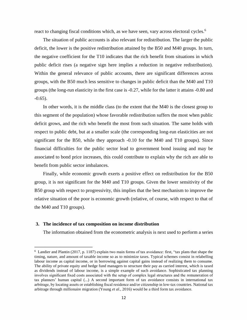
3.1. Obama’s administration

As reflected by the steep and steady rise of the tax composition ratio (Fig. 2a), fiscal

progressivity increased between 2009 and 2014 (last year in the sample period). Our first

exercise assesses to what extent such increase contributed to enhance redistribution from the

rich to the poor. For this, we simulate the estimated equations in two scenarios. A first one

in which the fiscal composition ratio takes its actual values (continuous line in Fig. 2a), and

a counterfactual scenario in which the departing situation is kept unchanged (dashed line in

Fig. 2a). The resulting counterfactual trajectories are the dashed ones plotted in Figs. 2b to

2d, which need to be compared to the actual ones (solid lines) in order to grasp the dynamic

contributions of the evolution of progressivity in that particular period.

Figure 2. Actual and simulated changes in redistribution.

a. Tax composition ratio b. Redistribution for the Bottom 50%

c. Redistribution for the Middle 40% d. Redistribution for the Top 10%

Note: Redistribution in Figures 2c to 2d is measured as percentage points increases in the post-tax

income shares.

0.70

0.75

0.80

0.85

0.90

0.95

1.00

2009 2010 2011 2012 2013 2014

0.71

0.97

Actual

evolution

Simulated

evolution0.715.8

6.0

6.2

6.4

6.6

6.8

7.0

2009 2010 2011 2012 2013 2014

5.8

6.8Actual

evolution

Simulated

evolution

6.2

0.3

0.4

0.5

0.6

0.7

0.8

0.9

1.0

1.1

1.2

2009 2010 2011 2012 2013 2014

0.4

1.1

Actual

evolution

Simulated

evolution

0.5

6.5

7.0

7.5

8.0

8.5

9.0

9.5

2009 2010 2011 2012 2013 2014

9.3

7.9

6.7

Simulated

evolution

Actual

evolution

14

Source: Piketty et al.’s (2018) for the actual trajectories; simulated paths based on estimated models.

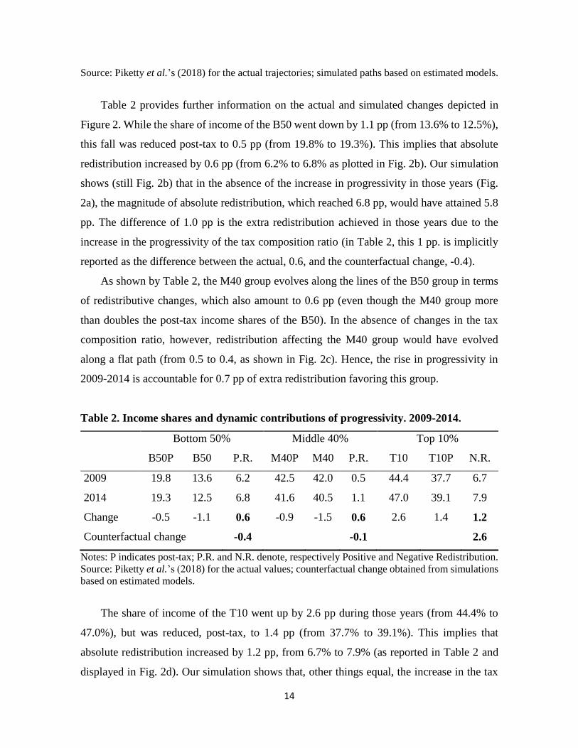
Table 2 provides further information on the actual and simulated changes depicted in

Figure 2. While the share of income of the B50 went down by 1.1 pp (from 13.6% to 12.5%),

this fall was reduced post-tax to 0.5 pp (from 19.8% to 19.3%). This implies that absolute

redistribution increased by 0.6 pp (from 6.2% to 6.8% as plotted in Fig. 2b). Our simulation

shows (still Fig. 2b) that in the absence of the increase in progressivity in those years (Fig.

2a), the magnitude of absolute redistribution, which reached 6.8 pp, would have attained 5.8

pp. The difference of 1.0 pp is the extra redistribution achieved in those years due to the

increase in the progressivity of the tax composition ratio (in Table 2, this 1 pp. is implicitly

reported as the difference between the actual, 0.6, and the counterfactual change, -0.4).

As shown by Table 2, the M40 group evolves along the lines of the B50 group in terms

of redistributive changes, which also amount to 0.6 pp (even though the M40 group more

than doubles the post-tax income shares of the B50). In the absence of changes in the tax

composition ratio, however, redistribution affecting the M40 group would have evolved

along a flat path (from 0.5 to 0.4, as shown in Fig. 2c). Hence, the rise in progressivity in

2009-2014 is accountable for 0.7 pp of extra redistribution favoring this group.

Table 2. Income shares and dynamic contributions of progressivity. 2009-2014.

Bottom 50% Middle 40% Top 10%

B50P B50 P.R. M40P M40 P.R. T10 T10P N.R.

2009 19.8 13.6 6.2 42.5 42.0 0.5 44.4 37.7 6.7

2014 19.3 12.5 6.8 41.6 40.5 1.1 47.0 39.1 7.9

Change -0.5 -1.1 0.6 -0.9 -1.5 0.6 2.6 1.4 1.2

Counterfactual change -0.4 -0.1 2.6

Notes: P indicates post-tax; P.R. and N.R. denote, respectively Positive and Negative Redistribution.

Source: Piketty et al.’s (2018) for the actual values; counterfactual change obtained from simulations

based on estimated models.

The share of income of the T10 went up by 2.6 pp during those years (from 44.4% to

47.0%), but was reduced, post-tax, to 1.4 pp (from 37.7% to 39.1%). This implies that

absolute redistribution increased by 1.2 pp, from 6.7% to 7.9% (as reported in Table 2 and

displayed in Fig. 2d). Our simulation shows that, other things equal, the increase in the tax

15

composition ratio during those years would have caused the negative redistribution to attain

9.3 pp rather than the actual 7.9 pp (Fig. 2d). The difference of 1.4 pp is the lost distributional

impact that would have been achieved in 2009-2014 had the behavioral response of the rich

on taxes stayed unchanged in those years. In other words, we ascribe this lost distributional

impact to the rich’s capacity to react to enhanced fiscal pressure. As discussed before,

enhanced access to professional services and advice (relative to the rest of the population)

would grant them the capacity to benefit from tax loopholes and tax havens so as to avoid as

much as possible unfriendly tax scenarios brought by Democrat governments.

It should be noted that the positive redistribution affecting the B50 and M40 jointly

amount to the negative redistribution on the T10 (6.2+0.5=6.7 in 2009; 6.8+1.1=7.9 in 2014).

This also holds in terms of changes (0.6+0.6=1.2) but with a much balanced distribution (note

that both in 2009 and 2014 the B50 group accounts for most of the redistribution from the

T10 rents). This implies that under Obama’s government, the B50 group did not benefit from

the extra redistribution from the rich to the poor in proportion to the existing redistributive

pattern.

In addition, our simulations imply that keeping the fiscal conditions as existing in 2009

regarding the aggregate tax composition and agents’ behavior would have resulted into a

mild loss of redistribution.7 This should come as no surprise since keeping the situation

unchanged implies reproducing the scenario in the absence of Obama’s policies and the rich’s

reaction to such redistributive policies. More precisely, keeping the scenario unchanged

would have caused the B50 and the M40 to loose around 0.4 and 0.1 pp of their post-tax

income shares (reported in Table 2 as the counterfactual change), in contrast to the actual 0.6

pp rise that both groups obtained. The rich, in turn, would have experienced a substantial rise

in their contribution (of 2.6 pp instead of 1.2 pp) had not covered themselves against

increased progressivity.8

7 The analysis below shows that such mild loss would have been along the lines of the one experienced in the

previous Republican period (2000-2008), which is consistent with the assumption of no changes that underlies

the simulation. 8 The reason why the addition of the impacts on the B50 and M40 do not add up to the one on the T10 is the

own nature of the exercise based on econometric estimates. There are differences in the estimated coefficient

of the tax composition ratio on redistribution across groups (B50, M40 and T10), but also in the persistence

coefficients (those on the lagged dependent variables). This, of course, is reflected in the dynamic simulations

and there is no reason why the addition of the simulated impacts should still match. Our method provides

insights based on the different behavioral responses of each group and is not a "decomposition" method.

16

Obama’s government was therefore successful in enhancing fiscal progressivity and

redistribution from the rich to the poor, but not fully efficient to the extent that the T10 rich

managed to scape 1.4 pp of extra negative redistribution.

3.2. Analysis across electoral cycles

Previous electoral cycles show clear differences in the aggregate distributive incidence

of the fiscal policy by type of government. Our results, therefore, confirm that party ideology

is not innocuous to tax progressivity.

Periods 1968-1976, 1980-1992 and 2000-2008 are characterized by at least two

consecutive Republican governments (three in 1980-1992). As reported in Table 3, a

common denominator characterizing these three periods is the scarce redistribution from the

Top 10% to the rest of the population. It was virtually nonexistent in 1968-1976 (0.1 pp),

small in 1980-1992 (0.6 pp), and even favorable to them in 2000-2008 (-0.2 pp). In contrast,

the two long periods with Democrats in government (1992-2000 and 2008-2014) saw an

increase of 1.7 and 1.2 pp in the share of income that was transferred to the B50 and M40

groups. Under Clinton’s presidency, most redistribution accrued to the M40 (1.6 pp), while

under Obama’s presidency it was symmetrically distributed (recall the 0.6 pp income share

gain of the B50 and M40).

Therefore, along the downward path documented for the tax composition ratio in Figure

1, which broadly reflects a steady loss in the redistributive power of the fiscal system, there

was a systematic bias towards the concentration of post-tax rents at the highest spectrum of

income distribution. This took place at the cost of the income shares of the Bottom 50%

(specially) and the Middle 40%.

Although it may seem striking that this two-headed phenomenon (poorer poor and richer

rich) has lasted for more than half a century, the analysis by electoral cycles reveals that the

compensating action from Democrat governments is actually unable to counterbalance the

policies implemented during Republican periods. Such phenomenon, which can be perceived

qualitatively by just looking at the fading peaks and troughs of the tax composition ratio

across time (Figure 1), is documented quantitatively through our simulations and the

resulting counterfactual changes also displayed in Table 3.9

9 The equivalent to Figure 2 has been produced for the rest of the periods explored (1968-1976; 1976-1980;

17

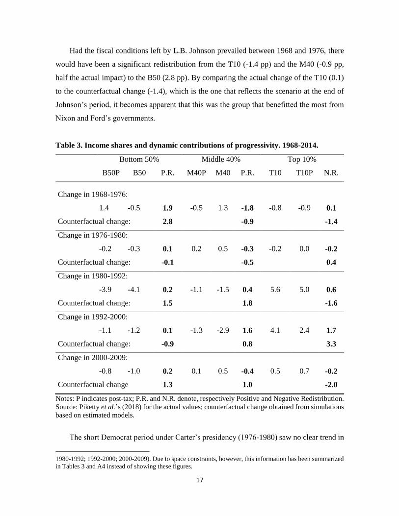
Had the fiscal conditions left by L.B. Johnson prevailed between 1968 and 1976, there

would have been a significant redistribution from the T10 (-1.4 pp) and the M40 (-0.9 pp,

half the actual impact) to the B50 (2.8 pp). By comparing the actual change of the T10 (0.1)

to the counterfactual change (-1.4), which is the one that reflects the scenario at the end of

Johnson’s period, it becomes apparent that this was the group that benefitted the most from

Nixon and Ford’s governments.

Table 3. Income shares and dynamic contributions of progressivity. 1968-2014.

Bottom 50% Middle 40% Top 10%

B50P B50 P.R. M40P M40 P.R. T10 T10P N.R.

Change in 1968-1976:

1.4 -0.5 1.9 -0.5 1.3 -1.8 -0.8 -0.9 0.1

Counterfactual change: 2.8 -0.9 -1.4

Change in 1976-1980:

-0.2 -0.3 0.1 0.2 0.5 -0.3 -0.2 0.0 -0.2

Counterfactual change: -0.1 -0.5 0.4

Change in 1980-1992:

-3.9 -4.1 0.2 -1.1 -1.5 0.4 5.6 5.0 0.6

Counterfactual change: 1.5 1.8 -1.6

Change in 1992-2000:

-1.1 -1.2 0.1 -1.3 -2.9 1.6 4.1 2.4 1.7

Counterfactual change: -0.9 0.8 3.3

Change in 2000-2009:

-0.8 -1.0 0.2 0.1 0.5 -0.4 0.5 0.7 -0.2

Counterfactual change 1.3 1.0 -2.0

Notes: P indicates post-tax; P.R. and N.R. denote, respectively Positive and Negative Redistribution.

Source: Piketty et al.’s (2018) for the actual values; counterfactual change obtained from simulations

based on estimated models.

The short Democrat period under Carter’s presidency (1976-1980) saw no clear trend in

1980-1992; 1992-2000; 2000-2009). Due to space constraints, however, this information has been summarized

in Tables 3 and A4 instead of showing these figures.

18

the tax income ratio. On the contrary, the policies held by Reagan and Bush father’s

governments kept pushing it down. As reported in Table 3, in the absence of such polices

(that is, in the scenario left by J. Carter’s administration), the rich would have contributed to

rebalance the functional income distribution by reducing their income share by 1.6 pp. The

difference is that instead of only the B50 benefiting from such redistribution (by 1.5 pp), the

M40 income share would have also benefited (by 1.8 pp). This further evidence confirms that

the T10 group benefited systematically from changes in the fiscal rules under the Republican

governments of Ford, Nixon, Reagan and Bush father.

Since 1992, Democrats dominated the political scene until Trump’s victory in November

2016. Amid many legislation changes, Clinton’s mandate saw tax cuts on low-income

families and tax increases on the wealthiest. In the absence of such changes, it is interesting

to observe that the B50 would have suffered more inequality than they actually did during

the roaring nineties. The counterfactual change (or, in other words, the scenario left by Bush

son) reveals a net contribution to the system of 0.9 pp, thereby enhancing this group’s fall in

terms of income share. In contrast, the rich would have contributed much more to

redistribution (by 3.3 pp) had they not eluded the more stringent fiscal conditions brought by

Clinton’s administration. They actually reduced their post-tax share by 1.7 pp, but the

model’s prediction is that they should have reduced their income shares twice as much, by

3.3 pp. The lost 1.6 pp is to be assigned to the rich’s ability to scape enhanced fiscal pressure.

In the next period it was Bush son who held the power. Our simulations for these years

indicate that had the fiscal system remained as it was left by Clinton’s administration, the

rich would have contributed by 2 extra pp to redistribution. Of these, 1.3 pp would have

benefited the B50 income’s share and 1.0 pp the M40’s one. The fiscal policies implemented

by Bush son prevented such redistribution to take place, as the actual fall in the T10 income

share was reduced to 0.2 pp. The difference between the counterfactual -2 pp versus the actual

-0.2 pp is the redistributive cost, in terms of functional income redistribution, of G.W. Bush

governments.

In other words, as indicated from our counterfactual analysis, during the last three

periods of Republican governments before Trump (28 years overall), the Top 10% benefited

from policies that prevented their income share to fall by 5 pp (=-1.4-1.6-2.0). In turn,

although Clinton and Obama’s administrations implemented policies that could have fully

19

counterbalanced this fall (3.3+2.6=5.9 pp), their actual compensating effect amounted to 1

pp (which is the actual change in redistribution experienced by the T10 group -0.2+1.2=1.0

pp). We ascribe the loss in the redistributive power of these policies to the ability of the rich

to deal with adverse fiscal conditions using all mechanisms brought by the market

liberalization and financial deregulation that started in the 1980s along with the acceleration

in economic globalization.

Note that these 5.0 percentage points (either those explained by the policies implemented

by the Republican governments, or those not effectively restored under the Democrats

administrations) account for 60% of the actual 8.3 pp increase of the income share

commanded by the Top 10%.

4. Conclusions

This paper takes a macroeconomic perspective to explore the incidence of tax

progressivity on income redistribution. In doing so, it combines time series data on major

public account items (different tax receipts, public deficit and public debt) with data on post-

tax and pre-tax income distribution from Piketty et al.’s (2018) novel database.

Two documented facts set the stage of the analysis. The first one is that the US tax system

is progressive (Mankiw, 2010). The second one is that the degree of progressivity shows a

secular tendency to weaken (Piketty and Saez, 2007; Hatgioannides et al., 2018). The

question we ask in that context is whether, and to what extent, this tendency has affected the

redistributive capacity of the fiscal system with regard to the Bottom 50%, Middle 40% and

Top 10% income shares.

We find that it has. The B50 have lost 21% of their income share and the M40 close to

10%, while the T10 have increased theirs by 28%. Republicans have shown little interest in

redistribution from the rich to the poor (and the middle class), while Democrats have tended

to enhance redistribution without succeeding to counterbalance neither the weakening trend

in the aggregate progressivity of the fiscal system, nor the falling trend of the B50 and M40

post-tax income shares.

We also find distributional losses that we associate to the rich’s capacity to protect

themselves, in terms of fiscal exposure, in periods in which tax progressivity augments (and

vice-versa). This is plausible to the extent that the rich are not only informed agents, but also

20

used (and therefore prepared) to deal with changing fiscal rules and opportunities.

Opportunities that take place both at the national level –on account of the fiscal changes

systematically brought by electoral cycles– and internationally –financial globalization has

made it possible to invest internationally in search of enhanced profitability which many

times is connected to fiscal benefits.

Given that party ideology will keep determining the redistributive scope of the fiscal

policies, it is important to set up mechanisms to avoid distributional losses. For this, extra

efforts and international coordination will be needed to restrict the proliferation of tax

loopholes and loose access to tax havens.

We suggest two avenues for future research. A first one relates to further disaggregating

the responses within the Middle 40% group, which will only be possible whenever new data

on the US DINA becomes available. Given that this group displays periods of positive and

negative redistribution, further disaggregation would shed light on the income decile after

which redistribution becomes unanimously negative. A second one is to investigate, along

the lines of Alstadsæter et al. (2017) for the Scandinavian countries, fiscal behavioral changes

when inequality increases; especially within the richer US Top 10% when confronted to

changing fiscal conditions.

References

Alstadsæter, A., N. Johannesen, and G. Zucman (2017): “Tax Evasion and Inequality”, NBER

Working Paper No. 23772, NBER, Massachusetts: Cambridge.

Ballard-Rosa, C., L. Martin, and K. Scheve (2017): “The Structure of American Income Tax

Policy Preferences”, The Journal of Politics, 79 (1), pp. 1-16.

Battisti, M. and J. Zeira (2016): “The Effects of Fiscal Redistribution” in K. Basu and J.E.

Stiglitz (Eds.) Inequality and Growth: Patterns and Policy, Vol. 1: Concepts and Analysis,

pp. 201-224, New York: Palgrave Macmillan.

Bierbrauer, F.J. and P.C. Boyer (2016): “Efficiency, Welfare, and Political Competition”,

The Quarterly Journal of Economics, 131 (1), pp. 461–518.

Borck, R. (2007): “Voting, inequality and redistribution”, Journal of Economic Surveys, 21

(1), pp. 90-109.

Diamond, P., and E. Saez (2011): “The Case for a Progressive Tax: From Basic Research to

Policy Recommendations”, Journal of Economic Perspectives, 25 (4), pp. 165-190.

Ferrier, J. (2010): Congressional Ambivalence: The Political Burdens of Constitutional

Authority, The University Press of Kentucky, Kentucky.

Guo, J.T. and A. Krause (2018): “Changing social preferences and optimal redistributive

taxation”, Oxford Economic Papers, 70 (1), pp. 73-92.

Herwartza, H., and B. Theilen (2017): “Ideology and redistribution through public spending”,

21

European Journal of Political Economy, 46, pp. 74–90.

Hatgioannides, J., M. Karanassou, and H. Sala (2018): “Should the Rich be Taxed More?

The Fiscal Inequality Coefficient”, Journal of Economic Issues, In Press.

Landier, A. and G. Plantin (2017): “Taxing the Rich”, Review of Economic Studies, 84, pp.

1186-1209.

Lebo, M.J. (2008): “Divided Government, United Approval: The Dynamics of Congressional

and Presidential Approval” Congress & the Presidency, 35 (2), pp. 1-16.

Mankiw, G.N. (2010): “Spreading the Wealth Around: Reflections Inspired by Joe the

Plumber”, Eastern Economic Journal, 36, pp. 285-298.

Mankiw, G.N., M.C. Weinzierl, and D. Yagan (2009): “Optimal Taxation in Theory and

Practice”, Journal of Economic Perspectives, 23 (4), pp. 147–174.

Pesaran, M.H. and Y. Shin (1999): “An Autoregressive Distributed-Lag Modelling Approach

to Cointegration Analysis” in Econometrics and Economic Theory in the Twentieth

Century: The Ragnar Frisch Centennial Symposium, edited by Strom, S., Cambridge

University Press, pp. 371-413.

Pesaran, M.H., Y. Shin, and Smith, R.J. (2001): “Bounds testing approaches to the analysis

of level relationships”, Journal of Applied Econometrics, 16, pp. 289-326.

Piketty, T. and E. Saez, (2007): “How Progressive is the U.S. Federal Tax System? A

Historical and International Perspective”, Journal of Economic Perspectives, 21 (1), pp.

3-24.

Piketty, T., E. Saez, and G. Zucman (2018): “Distributional National Accounts: Methods and

Estimates for the United States”, Quarterly Journal of Economics, 133 (2), pp. 553-609.

Romer, C.D. and D.H. Romer (2010): “The Macroeconomic Effects of Tax Changes:

Estimates Based on a New Measure of Fiscal Shocks”, American Economic Review, 100

(2), PP. 763–801.

Solt, F. (2016): “The Standardized World Income Inequality Database”, Social Science

Quarterly, 97(5), pp. 1267-1281.

Scheve, K. and D. Stasavage (2016): Taxing the Rich: A History of Fiscal Fairness in the

United States and Europe, Princeton University Press: Princeton.

Sussman, G. and B.W. Daynes (1995): “The Impact of Political Ideology on Congressional

Support for Presidential Policy Making Authority: The Case of the Fast Track”, Congress

& the Presidency, 22 (2), pp. 141-153.

Young, C., C. Varner, I.Z. Lurie, and R. Prisinzano (2016): “Millionaire Migration and

Taxation of the Elite: Evidence from Administrative Data”, American Sociological

Review, 81(3), pp. 421–446.

22

APPENDICES

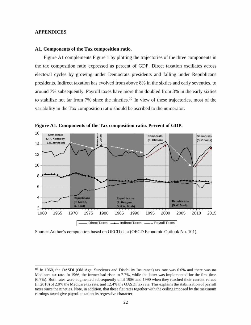
A1. Components of the Tax composition ratio.

Figure A1 complements Figure 1 by plotting the trajectories of the three components in

the tax composition ratio expressed as percent of GDP. Direct taxation oscillates across

electoral cycles by growing under Democrats presidents and falling under Republicans

presidents. Indirect taxation has evolved from above 8% in the sixties and early seventies, to

around 7% subsequently. Payroll taxes have more than doubled from 3% in the early sixties

to stabilize not far from 7% since the nineties.10 In view of these trajectories, most of the

variability in the Tax composition ratio should be ascribed to the numerator.

Figure A1. Components of the Tax composition ratio. Percent of GDP.

2

4

6

8

10

12

14

16

1960 1965 1970 1975 1980 1985 1990 1995 2000 2005 2010 2015

Direct Taxes Indirect Taxes Payroll Taxes

Democrats

(B. Clinton)

Republicans

(R. Nixon,

G. Ford)

De

mo

cra

ts

(J. C

art

er)Democrats

(J.F. Kennedy,

L.B. Johnson)

Republicans

(R. Reagan,

G.H.W. Bush)

Republicans

(G.W. Bush)

Democrats

(B. Obama)

Source: Author’s computation based on OECD data (OECD Economic Outlook No. 101).

10 In 1960, the OASDI (Old Age, Survivors and Disability Insurance) tax rate was 6.0% and there was no

Medicare tax rate. In 1966, the former had risen to 7.7%, while the latter was implemented for the first time

(0.7%). Both rates were augmented subsequently until 1986 and 1990 when they reached their current values

(in 2018) of 2.9% the Medicare tax rate, and 12.4% the OASDI tax rate. This explains the stabilization of payroll

taxes since the nineties. Note, in addition, that these flat rates together with the ceiling imposed by the maximum

earnings taxed give payroll taxation its regressive character.

23

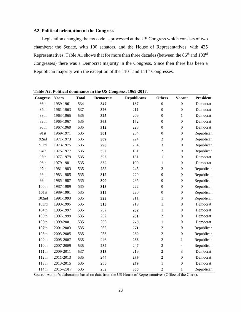
A2. Political orientation of the Congress

Legislation changing the tax code is processed at the US Congress which consists of two

chambers: the Senate, with 100 senators, and the House of Representatives, with 435

Representatives. Table A1 shows that for more than three decades (between the 86th and 103rd

Congresses) there was a Democrat majority in the Congress. Since then there has been a

Republican majority with the exception of the 110th and 111th Congresses.

Table A2. Political dominance in the US Congress. 1969-2017.

Congress Years Total Democrats Republicans Others Vacant President

86th 1959-1961 534 347 187 0 0 Democrat

87th 1961-1963 537 326 211 0 0 Democrat

88th 1963-1965 535 325 209 0 1 Democrat

89th 1965-1967 535 363 172 0 0 Democrat

90th 1967-1969 535 312 223 0 0 Democrat

91st 1969-1971 535 301 234 0 0 Republican

92nd 1971-1973 535 309 224 2 0 Republican

93rd 1973-1975 535 298 234 3 0 Republican

94th 1975-1977 535 352 181 2 0 Republican

95th 1977-1979 535 353 181 1 0 Democrat

96th 1979-1981 535 335 199 1 0 Democrat

97th 1981-1983 535 288 245 2 0 Republican

98th 1983-1985 535 315 220 0 0 Republican

99th 1985-1987 535 300 235 0 0 Republican

100th 1987-1989 535 313 222 0 0 Republican

101st 1989-1991 535 315 220 0 0 Republican

102nd 1991-1993 535 323 211 1 0 Republican

103rd 1993-1995 535 315 219 1 0 Democrat

104th 1995-1997 535 252 282 1 0 Democrat

105th 1997-1999 535 252 281 2 0 Democrat

106th 1999-2001 535 256 278 1 0 Democrat

107th 2001-2003 535 262 271 2 0 Republican

108th 2003-2005 535 253 280 2 0 Republican

109th 2005-2007 535 246 286 2 1 Republican

110th 2007-2009 535 282 247 2 4 Republican

111th 2009-2011 537 313 219 2 3 Democrat

112th 2011-2013 535 244 289 2 0 Democrat

113th 2013-2015 535 255 279 1 0 Democrat

114th 2015–2017 535 232 300 2 1 Republican

Source: Author’s elaboration based on data from the US House of Representatives (Office of the Clerk).

24

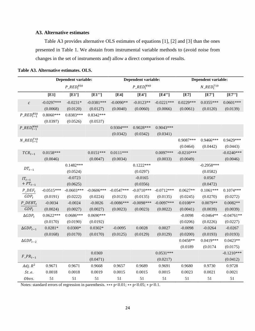
A3. Alternative estimates

Table A3 provides alternative OLS estimates of equations [1], [2] and [3] than the ones

presented in Table 1. We abstain from instrumental variable methods to (avoid noise from

changes in the set of instruments and) allow a direct comparison of results.

Table A3. Alternative estimates. OLS.

Dependent variable: Dependent variable: Dependent variable:

𝑃_𝑅𝐸𝐷𝑡𝐵50 𝑃_𝑅𝐸𝐷𝑡

𝑀40 𝑁_𝑅𝐸𝐷𝑡𝑇10

[E1] [E1’] [E1’’] [E4] [E4’] [E4’’] [E7] [E7’] [E7’’]

𝑐 -0.0297*** -0.0231* -0.0381*** -0.0090** -0.0123** -0.0221*** 0.0229*** 0.0355*** 0.0601***

(0.0068) (0.0120) (0.0127) (0.0040) (0.0060) (0.0066) (0.0061) (0.0120) (0.0139)

𝑃_𝑅𝐸𝐷𝑡−1𝐵50 0.8060*** 0.8383*** 0.8342***

(0.0397) (0.0526) (0.0537)

𝑃_𝑅𝐸𝐷𝑡−1𝑀40 0.9304*** 0.9028*** 0.9043***

(0.0342) (0.0342) (0.0341)

𝑁_𝑅𝐸𝐷𝑡−1𝑇10 0.9087*** 0.9466*** 0.9429***

(0.0464) (0.0442) (0.0443)

𝑇𝐶𝑅𝑡−1 0.0158*** 0.0151*** 0.0111*** 0.0097*** -0.0210*** -0.0240***

(0.0046) (0.0047) (0.0034) (0.0033) (0.0049) (0.0046)

𝐷𝑇𝑡−1 0.1482*** 0.1222*** -0.2958***

(0.0524) (0.0297) (0.0582)

𝐼𝑇𝑡−1

+ 𝑃𝑇𝑡−1

-0.0723 -0.0165 0.0567

(0.0625) (0.0356) (0.0472)

𝑃_𝐷𝐸𝐹𝑡

𝐺𝐷𝑃𝑡

-0.0515*** -0.0603*** -0.0606*** -0.0547*** -0.0710*** -0.0712*** 0.0627** 0.1061*** 0.1074***

(0.0191) (0.0222) (0.0224) (0.0123) (0.0135) (0.0135) (0.0245) (0.0270) (0.0272)

𝑃_𝐷𝐸𝐵𝑇𝑡

𝐺𝐷𝑃𝑡

-0.0034 -0.0024 -0.0026 -0.0086*** -0.0098*** -0.0097*** 0.0108** 0.0079** 0.0082**

(0.0024) (0.0027) (0.0027) (0.0023) (0.0023) (0.0022) (0.0041) (0.0039) (0.0039)

∆𝐺𝐷𝑃𝑡 0.0622*** 0.0686*** 0.0690*** -0.0098 -0.0464** -0.04761**

(0.0170) (0.0190) (0.0192) (0.0206) (0.0226) (0.0227)

∆𝐺𝐷𝑃𝑡−1 0.0281* 0.0300* 0.0302* -0.0095 0.0028 0.0027 -0.0098 -0.0264 -0.0267

(0.0168) (0.0170) (0.0170) (0.0125) (0.0129) (0.0129) (0.0200) (0.0193) (0.0193)

∆𝐺𝐷𝑃𝑡−2 0.0458** 0.0419*** 0.0423**

(0.0189 (0.0174 (0.0175)

𝐹_𝑃𝑅𝑡−1 0.0369 0.0531*** -0.1210***

(0.0471) (0.0217) (0.0412)

𝐴𝑑𝑗. 𝑅2 0.9671 0.9671 0.9668 0.9657 0.9689 0.9691 0.9680 0.9730 0.9728

𝑆𝑡. 𝑒. 0.0018 0.0018 0.0019 0.0015 0.0015 0.0015 0.0023 0.0021 0.0021

𝑂𝑏𝑣𝑠. 51 51 51 51 51 51 51 51 51

Notes: standard errors of regression in parenthesis. ∗∗∗ p<0.01; ∗∗ p<0.05; ∗ p<0.1.

25

The first alternative substitutes the Tax composition ratio by its numerator (𝐷𝑇𝑡) and

denominator (𝐼𝑇𝑡 + 𝑃𝑇𝑡), which are introduced as separate controls in models [E1’], [E4’]

and [E7’]. The three variables (𝐷𝑇; 𝐼𝑇; 𝑃𝑇) are expressed as percent of GDP. Direct taxation,

which is characterized by its variability (Figure A1), is fully significant in the three models,

in contrast to indirect and payroll taxes. Direct taxation, therefore, appears as a key driving

factor of the overall progressivity of the system.

The second alternative includes fiscal pressure ( 𝐹_𝑃𝑅𝑡 = 𝐷𝑇𝑡 + 𝐼𝑇𝑡 + 𝑃𝑇𝑡 ) as an

additional control. Hence, beyond controlling for public deficit and debt, we impose a further

restriction so that the overall level of taxation is kept constant. All three estimated models,

[E1’’], [E4’’] and [E7’’], deliver a common picture in which the estimated coefficient of the

Tax composition ratio is fully robust. In addition, we observe that this additional control is

not significant to explain redistribution affecting the B50 income shares, but it is so in terms

of the M40 and T10 ones. Thus, for a given level of overall progressivity (𝑇𝐶𝑅 is a control

in the regression), more fiscal pressure benefits the M40 and T10 income shares, but not the

poor. The fact that a higher level of fiscal pressure with no further progressivity reduces the

negative redistribution affecting the T10 income shares points to the ability of these rents to

scape taxes, as documented in Young et al. (2016) and Landier and Plantin (2017).

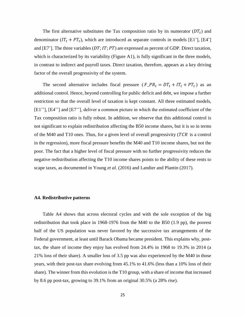
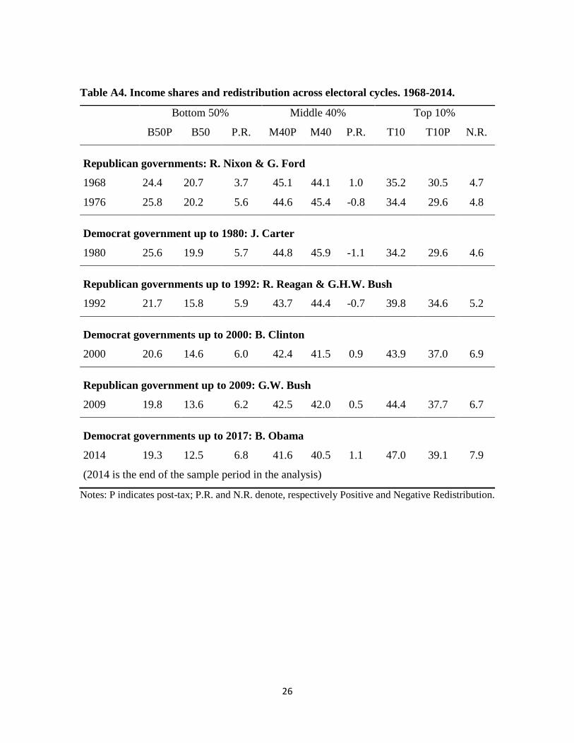
A4. Redistributive patterns

Table A4 shows that across electoral cycles and with the sole exception of the big

redistribution that took place in 1968-1976 from the M40 to the B50 (1.9 pp), the poorest

half of the US population was never favored by the successive tax arrangements of the

Federal government, at least until Barack Obama became president. This explains why, post-

tax, the share of income they enjoy has evolved from 24.4% in 1968 to 19.3% in 2014 (a

21% loss of their share). A smaller loss of 3.5 pp was also experienced by the M40 in those

years, with their post-tax share evolving from 45.1% to 41.6% (less than a 10% loss of their

share). The winner from this evolution is the T10 group, with a share of income that increased

by 8.6 pp post-tax, growing to 39.1% from an original 30.5% (a 28% rise).

26

Table A4. Income shares and redistribution across electoral cycles. 1968-2014.

Bottom 50% Middle 40% Top 10%

B50P B50 P.R. M40P M40 P.R. T10 T10P N.R.

Republican governments: R. Nixon & G. Ford

1968 24.4 20.7 3.7 45.1 44.1 1.0 35.2 30.5 4.7

1976 25.8 20.2 5.6 44.6 45.4 -0.8 34.4 29.6 4.8

Democrat government up to 1980: J. Carter

1980 25.6 19.9 5.7 44.8 45.9 -1.1 34.2 29.6 4.6

Republican governments up to 1992: R. Reagan & G.H.W. Bush

1992 21.7 15.8 5.9 43.7 44.4 -0.7 39.8 34.6 5.2

Democrat governments up to 2000: B. Clinton

2000 20.6 14.6 6.0 42.4 41.5 0.9 43.9 37.0 6.9

Republican government up to 2009: G.W. Bush

2009 19.8 13.6 6.2 42.5 42.0 0.5 44.4 37.7 6.7

Democrat governments up to 2017: B. Obama

2014 19.3 12.5 6.8 41.6 40.5 1.1 47.0 39.1 7.9

(2014 is the end of the sample period in the analysis)

Notes: P indicates post-tax; P.R. and N.R. denote, respectively Positive and Negative Redistribution.