Dissolution Methodologies and IVIVC - UVmbermejo/DissolutionC.pdf · Dissolution test ODD Lake...
29
ODD Lake Tahoe. March 2002. Dissolution and IVIVC 1 © Prof. Bermejo Dept. of Pharmaceutics Dissolution Methodologies and IVIVC Marival Bermejo,Ph.D. Dept. Farmacia y Tecnología Farmacéutica Facultad de Farmacia. Universidad de Valencia España ODD Lake Tahoe. March 2002. Dissolution and IVIVC 2 © Prof. Bermejo Dept. of Pharmaceutics Dissolution Methodologies and IVIVC < Dissolution testing and BCS < IVIVC: - Definition and Levels - Development • Calculation of fraction absorbed • Mathematical modeling - Validation: predictability analysis - Approached to obtain IVIVC • Non linear Mathematical models • Biorelevant Dissolution media < Curve comparison
-
Upload
truongmien -
Category
Documents
-
view
214 -
download
0
Transcript of Dissolution Methodologies and IVIVC - UVmbermejo/DissolutionC.pdf · Dissolution test ODD Lake...

1
ODD Lake Tahoe. March 2002. Dissolution and IVIVC
1© Prof. BermejoDept. of Pharmaceutics
Dissolution Methodologies and IVIVC
Marival Bermejo,Ph.D.Dept. Farmacia y Tecnología Farmacéutica
Facultad de Farmacia. Universidad de Valencia
España
ODD Lake Tahoe. March 2002. Dissolution and IVIVC
2© Prof. BermejoDept. of Pharmaceutics
Dissolution Methodologies and IVIVC
< Dissolution testing and BCS< IVIVC:
− Definition and Levels− Development
• Calculation of fraction absorbed• Mathematical modeling
− Validation: predictability analysis− Approached to obtain IVIVC
• Non linear Mathematical models• Biorelevant Dissolution media
< Curve comparison

2
ODD Lake Tahoe. March 2002. Dissolution and IVIVC
3© Prof. BermejoDept. of Pharmaceutics
ODD Lake Tahoe. March 2002. Dissolution and IVIVC
4© Prof. BermejoDept. of Pharmaceutics
Factors influencing dissolution rate
< Noyes Whitney equation
( )s tQ A D
C Ct h
∂ ⋅= ⋅ −
∂

3
ODD Lake Tahoe. March 2002. Dissolution and IVIVC
5© Prof. BermejoDept. of Pharmaceutics
Factors influencing dissolution rate
Volume of GI fluids: secretions
pH,surfactants
Viscosity of GI fluids
GI motility
Presence of surfactants
Physiological variable
Volume of medium
Ct
pH, surfactantshydrophilicityCs
Viscosity of medium
Molecular sizeD
Stirring rateSystem hydrodynamics
h
Presence of surfactants
Particle sizeA
In vitro factorPhysico-chemicalcharacteristic
Parameter
ODD Lake Tahoe. March 2002. Dissolution and IVIVC
6© Prof. BermejoDept. of Pharmaceutics
Dissolution test
< Quality control:− Process control− Batch-to-batch quality
< Predictor of Product performance In vivo
BCS

4
ODD Lake Tahoe. March 2002. Dissolution and IVIVC
7© Prof. BermejoDept. of Pharmaceutics
Biowaiver: permission to use dissolution test as a surrogate of pharmacokinetic data:
< For accepting product sameness under SUPAC-related changes.
< To waive bioequivalence requirements for lower strengths of a dosage form.
< To support waivers for other bioequivalence requirements.
Dissolution test
ODD Lake Tahoe. March 2002. Dissolution and IVIVC
8© Prof. BermejoDept. of Pharmaceutics
J P C= ⋅
PermeabilitySolubility andDissolution rate In vivoLuminal degradation
•Same dissolution profile•Formulation components do not alter permeability or intestinal transit

5
ODD Lake Tahoe. March 2002. Dissolution and IVIVC
9© Prof. BermejoDept. of Pharmaceutics
Class IV: LS/LP
Furosemide, Hydrochlorothiazide
Class III:HS/LP
Ranitidine, Cimetidine, Atenolol
Class II:LS/HP
Carbamazepine, Ketoprofen, Naproxen
Class I:HS/HP
Verapamil, ProparanololMetoprolol
Perm
eabi
lity
Volume of aqueous buffer to dissolve the highest dose
ODD Lake Tahoe. March 2002. Dissolution and IVIVC
10© Prof. BermejoDept. of Pharmaceutics

6
ODD Lake Tahoe. March 2002. Dissolution and IVIVC
11© Prof. BermejoDept. of Pharmaceutics
ODD Lake Tahoe. March 2002. Dissolution and IVIVC
12© Prof. BermejoDept. of Pharmaceutics
IVIVC Definition
< An In-vitro in-vivo correlation (IVIVC) has been defined by the Food and Drug Administration (FDA) as “a predictive mathematical model describing the relationship between an in-vitro property of a dosage form and an in-vivo response”.

7
ODD Lake Tahoe. March 2002. Dissolution and IVIVC
13© Prof. BermejoDept. of Pharmaceutics
< Bioequivalent drug products : Pharmaceutical equivalents or pharmaceutical alternatives whose rate and extent of absorption do not show a significant difference when administered at the same molar dose of the therapeutic moiety under similar experimental conditions, either single dose or multiple dose. (27 CFR 320.1(e)).
ODD Lake Tahoe. March 2002. Dissolution and IVIVC
14© Prof. BermejoDept. of Pharmaceutics
Methods for assessing BE1
< Pharmacokinetic study< Pharmacodynamic study< Comparative clinical study< In vitro study
1.GUIDANCE FOR INDUSTRYBioavailability and Bioequivalence Studies for Orally Administered Drug Products
— General Considerations

8
ODD Lake Tahoe. March 2002. Dissolution and IVIVC
15© Prof. BermejoDept. of Pharmaceutics
< The main objective of developing and evaluating an IVIVC is to establish the dissolution test as a surrogate for human bioequivalence studies, which may reduce the number of bioequivalence studies performed during the initial approval process as well as with certain scale-up and post approval changes.
ODD Lake Tahoe. March 2002. Dissolution and IVIVC
16© Prof. BermejoDept. of Pharmaceutics
IVIVC Levels
< Level A correlation is a point to point relationship between in vitro dissolution and the in vivo absorption rate of a drug from the dosage form.
< Level B compares the mean in vitro dissolution time (MDTvitro) to the mean in vivo dissolution time (MDTvivo).
< Level C is a single point comparison of the amount of drug dissolved at one dissolution time point to one pharmacokinetic parameter.
< Multiple Level C is a correlation involving one or several pharmacokinetic parameters to the amount of drug dissolved at various time points.

9
ODD Lake Tahoe. March 2002. Dissolution and IVIVC
17© Prof. BermejoDept. of Pharmaceutics
Level A correlation
Adapted from Sirisuth N and Eddington N.Int. J. Generic Drugs (IVIVC series part III)
Fdiss
0.0 0.2 0.4 0.6 0.8 1.0 1.2
Fab
s
-0.2
0.0
0.2
0.4
0.6
0.8
1.0
1.2
ODD Lake Tahoe. March 2002. Dissolution and IVIVC
18© Prof. BermejoDept. of Pharmaceutics
Level B correlation
MDT vitro (hours)
1.1 1.2 1.3 1.4 1.5 1.6 1.7 1.8
MR
T v
ivo
(hou
rs)
12
14
16
18
20
22
24
26
28
Adapted from Sirisuth N and Eddington N.Int. J. Generic Drugs (IVIVC series part III)

10
ODD Lake Tahoe. March 2002. Dissolution and IVIVC
19© Prof. BermejoDept. of Pharmaceutics
MDT(hours)0 1 2 3 4 5 6
AU
C(n
g·h/
mL)
4000
6000
8000
10000
12000
Adapted from Balan G et al. J.Pharm Sci 90(8)1176-1185.(2001)
Level C correlation
ODD Lake Tahoe. March 2002. Dissolution and IVIVC
20© Prof. BermejoDept. of Pharmaceutics
Development of IVIVC: level AOne step approachTwo steps approach
Ødevelop formulations with different release rates, such as slow, medium, fast; Øobtain in vitro dissolution profiles and in vivo plasma concentration profiles for these formulations
§estimate the in vivo absorption or dissolution time course using an appropriate technique for each formulation and subject.
§Establish the Link model between in vivo and in vitro variable§Predict plasma concentration from in vitro data using the Link model
Step
1St
ep 2
§Predict plasma concentration from in vitro profile using a LINK model whose parameters are fitted in one step
•Do not involve deconvolution•Link model is not determined separately•Can be done without a reference (IV bolus, oral solution or IR form)

11
ODD Lake Tahoe. March 2002. Dissolution and IVIVC
21© Prof. BermejoDept. of Pharmaceutics
In vitro Dissolution
0.020.040.060.080.0
100.0120.0
0 100 200 300
time (min)
Am
ount
Rel
ease
d %
In vivo Absorption
0.020.040.060.080.0
100.0120.0
0 100 200 300
time (min)
Am
ount
abs
or. %
Plasma levels
0
10
20
30
40
50
0 100 200 300 400
time(min)
plas
ma
conc
.
IVIVC
Amount dissolved %
0 20 40 60 80 100
Am
ount
abs
orbe
d %
0
20
40
60
80
100
?
ODD Lake Tahoe. March 2002. Dissolution and IVIVC
22© Prof. BermejoDept. of Pharmaceutics
Assumptions:Linear dispositionLinear first passLinear absorption

12
ODD Lake Tahoe. March 2002. Dissolution and IVIVC
23© Prof. BermejoDept. of Pharmaceutics
Determining the fraction of dose absorbed
< Model dependent methods− Wagner Nelson Equation− Loo-Riegelman Method
< Model independent methods− Deconvolution
ODD Lake Tahoe. March 2002. Dissolution and IVIVC
24© Prof. BermejoDept. of Pharmaceutics
0 at ct et
tct d et el d
Q Q Q
Q C V Q k V AUC
= +
= ⋅ = ⋅ ⋅
0
0
tat t d el d
a el d
Q C V k V AUC
Q k V AUC∞∞
= ⋅ + ⋅ ⋅
= ⋅ ⋅
0 tt t d el d
el d o
at d ct d et d
Q C V k V AUCQ k V AUC
Q V Q V Q V
∞∞
⋅ + ⋅ ⋅=
⋅ ⋅
= +
< Wagner Nelson: Mass balance

13
ODD Lake Tahoe. March 2002. Dissolution and IVIVC
25© Prof. BermejoDept. of Pharmaceutics
0
fraction remaining to be absorbed
t c e
tt t el
el o
t
A A A
A C k AUCA k AUC
AA
∞∞
∞
= +
+ ⋅=
⋅
=1-
< Wagner Nelson: Mass balance
1.0
21.0
41.0
61.0
81.0
101.0
121.0
0 50 100 150 200 250 300
time ( min)
At
(mg
/mL
)
1.0
10.0
100.0
0 50 100 150 200 250 300
time ( min)
At (
mg
/mL
)
ln(100 ) ln100 ta
Ak t
A∞
− = − ⋅ (100 ) 100ta
Ak t
A∞
− = − ⋅
ODD Lake Tahoe. March 2002. Dissolution and IVIVC
26© Prof. BermejoDept. of Pharmaceutics
Time (min) C(mg/mL)5 2.29 0.55 0.55
10 4.22 2.11 1.0115 5.83 2.92 1.4030 9.29 4.64 2.2345 11.33 5.66 2.7260 12.54 6.27 3.0190 5.00 6.84 3.28 30
120 1.75 7.04 3.38 60150 0.61 2.50 3.41 90180 0.21 0.87 3.42 120210 0.07 0.31 3.43 150240 0.03 0.11 3.43 180270 0.01 0.04 1.20 210300 0.00 0.01 0.42 240330 0.00 0.00 0.15 270360 0.00 0.00 0.05 300390 0.00 0.00 0.02 330420 0.00 0.00 0.01 360
ko(mg/mL*min) 0.50 0.25 0.12 ko(calc) -0.4664 -0.2469 -0.1229kel(min-1) 0.04 Vd(L) 10t1/2(min) 19.80cinf 14.29 7.14 3.43
plasma levels
0.00
0.00
0.01
0.10
1.00
10.00
100.00
0 100 200 300 400 500time (min)
con
c m
g/m
L
Wagner Nelson Plot
0.00
20.00
40.00
60.00
80.00
100.00
120.00
0 100 200 300 400 500
time (min)
At/A
inf
(100 ) 100ta
Ak t
A∞
− = − ⋅

14
ODD Lake Tahoe. March 2002. Dissolution and IVIVC
27© Prof. BermejoDept. of Pharmaceutics
Time (min) C(mg/mL)5 0.39 0.20 0.10
10 0.72 0.38 0.1915 1.01 0.55 0.2830 1.65 0.98 0.5245 2.03 1.30 0.7260 2.24 1.54 0.8990 2.35 1.83 1.15
120 2.26 1.94 1.32150 2.08 1.94 1.42180 1.89 1.87 1.47210 1.69 1.76 1.48240 1.51 1.63 1.46270 1.34 1.50 1.42300 1.19 1.36 1.36330 1.06 1.23 1.29360 0.94 1.11 1.22390 0.83 0.99 1.14420 0.74 0.89 1.06
ka min-1 0.025 0.013 0.006 ka(calc)min-1 -0.0250 -0.0126 -0.0069kel(min-1) 0.004t1/2(min) 173.25Vd 30.00D 100.00
plasma levels
0.10
1.00
10.00
0 100 200 300 400time (min)
con
c m
g/m
L
Wagner Nelson Plot
0.00
20.00
40.00
60.00
80.00
100.00
120.00
0 100 200 300 400 500
time (min)
At/
Ain
f
ln(100 ) ln100 ta
Ak t
A∞
− = − ⋅
ODD Lake Tahoe. March 2002. Dissolution and IVIVC
28© Prof. BermejoDept. of Pharmaceutics
Time (min) C(mg/mL)5 0.30 0.155 0.076
10 0.44 0.236 0.11815 0.49 0.276 0.14130 0.45 0.294 0.16245 0.36 0.269 0.16060 0.28 0.240 0.15590 0.18 0.191 0.144
120 0.12 0.155 0.132150 0.09 0.127 0.121180 0.07 0.105 0.111210 0.06 0.088 0.101240 0.05 0.074 0.091270 0.05 0.063 0.083300 0.04 0.054 0.075330 0.03 0.047 0.068360 0.03 0.041 0.061390 0.03 0.035 0.055420 0.02 0.031 0.049
ka min-1 0.025 0.013 0.006 alfa 0.113781 ka (calc)min-1 #¡VALOR! #¡VALOR! -0.0122k10(min-1) 0.0600 Vc 30.00 beta 0.004219k12 min-1 0.0500k21 min-1 0.0080D 100.00
Plasma levels
0.01
0.10
1.00
10.00
0 100 200 300 400time (min)
Con
c m
g/m
L
Wagner Nelson Plot
1.00
51.00
101.00
151.00
201.00
251.00
0 100 200 300 400 500
time (min)
At/A
inf
ka k10
k21k12A C E= +

15
ODD Lake Tahoe. March 2002. Dissolution and IVIVC
29© Prof. BermejoDept. of Pharmaceutics
< Loo-Riegelman: Mass balance
c e pa
c c
t t t t
Q Q QQV V
A C E P
+ +=
= + +
21 21
21 21
10 0
12 0
12 121 1
21
(1 )2
tt t t
tk t k tt
k t k tt t t
A C k AUC P
P k e C e t
k kP P e C e C t
k
− ⋅ ⋅
− ⋅∆ − ⋅∆− −
= + ⋅ +
= ⋅ ⋅ ⋅ ∂
= ⋅ + ⋅ − + ⋅∆ ⋅ ∆
∫
Parameters obtained from IV dataIV and oral administration with the same subjects
ODD Lake Tahoe. March 2002. Dissolution and IVIVC
30© Prof. BermejoDept. of Pharmaceutics
Time (min) C(mg/mL)5 0.30 0.155 0.076
10 0.44 0.236 0.11815 0.49 0.276 0.14130 0.45 0.294 0.16245 0.36 0.269 0.16060 0.28 0.240 0.15590 0.18 0.191 0.144
120 0.12 0.155 0.132150 0.09 0.127 0.121180 0.07 0.105 0.111210 0.06 0.088 0.101240 0.05 0.074 0.091270 0.05 0.063 0.083300 0.04 0.054 0.075 330 0.03 0.047 0.068360 0.03 0.041 0.061390 0.03 0.035 0.055420 0.02 0.031 0.049
ka min-1 0.025 0.013 0.006 alfa 0.113781 ka(calc)min-1 -0.0242 -0.0122 -0.0062k10(min-1) 0.0600 Vc 30.00 beta 0.004219k12 min-1 0.0500k21 min-1 0.0080D 100.00
plasma levels
0.01
0.10
1.00
10.00
0 100 200 300 400time (min)
con
c m
g/m
L
Loo-Riegelman Plot
0.00
20.00
40.00
60.00
80.00
100.00
120.00
0 100 200 300 400 500
time (min)
At/
Ain
f
ka k10
k21k12A C E P= + +

16
ODD Lake Tahoe. March 2002. Dissolution and IVIVC
31© Prof. BermejoDept. of Pharmaceutics
Input Response
Rat
e
time timeτo τo
Amount=1
δ(t): unit impulse 1·cδ(t):unit impulse response
time timeτo τoτ1 τ1
a·δ(t-τ1) a·cδ(t-τ1)
time timeτo τoτ1 τ1
a·δ(t-τo)+b·δ(t -τ1) a·cδ(t-τ0)+b·cδ(t-τ1)
a b
conc
entr
atio
n
superposition
Time invariancetime timeτo
τo
a·δ(t) a·cδ(t)Amount=a
ODD Lake Tahoe. March 2002. Dissolution and IVIVC
32© Prof. BermejoDept. of Pharmaceutics
time timeτo τoτ1 τ1
a*δ(t-τo)+b* δ(t -τ1) a*cδ(t-τ0)+b* cδ(t-τ1)
a b
time timeτo τoτn τ1
Rat
e
Con
cent
ratio
n
Amount= f(τn)∆τC(t)= [f(τo) ∆τ]·cδ(t-τo)+
[f(τ1) ∆τ]·cδ(t-τ1)+….[f(τn) ∆τ]·cδ(t-τn)=
,
0
( ) ( ) ( )
0
n n t
nn
c t f c tτ
δτ τ τ
τ
= =
=
= ⋅ − ⋅ ∆
∆ →
∑
0
( ) ( ) ( )t
c t f c t dδτ τ τ= ⋅ − ⋅∫response impulse Unit impulse response

17
ODD Lake Tahoe. March 2002. Dissolution and IVIVC
33© Prof. BermejoDept. of Pharmaceutics
Methods of Deconvolution
< Analytic: Laplace transforms< Implicit: deconvolution by curve fitting< Numeric: point-area
Convolution: solving c(t) given f(t) and cδ(t)Deconvolution: solving f(t) given cδ(t) and c(t)
or solving cδ(t) given f(t) and c(t)
ODD Lake Tahoe. March 2002. Dissolution and IVIVC
34© Prof. BermejoDept. of Pharmaceutics
Laplace transform
( ){ } ( ) ( )0
s tf t F s e f t t∞
− ⋅= = ⋅ ⋅ ∂∫l

18
ODD Lake Tahoe. March 2002. Dissolution and IVIVC
35© Prof. BermejoDept. of Pharmaceutics
0
( ) ( ) ( )t
c t f c t dδτ τ τ= ⋅ − ⋅∫response input Unit impulse response
[ ] [ ][ ] [ ] [ ]
1( ) ( ) ( )
( ) ( ) ( )
( ) ( ) ( )
c t f t c t
c t f t c t
C s F s C s
δ
δ
δ
− = ⋅ = ⋅
= ⋅
l l ll l l
<Analytic: Laplace transforms
[ ]
[ ]
( ) ( ) ( )
1 1( ) ( ) ( )
( )
a
el
k t aa
a
k t
d d el
F D kf t F D k e f t
s k
Dc t e c t
D V V s kδ δ
− ⋅
− ⋅
⋅ ⋅= ⋅ ⋅ ⋅ =
+
= ⋅ ⋅ =⋅ +
l
l
[ ] [ ]
1
( ) ( )( ) ( )
( )( ) ( ) ( )
el a
a
d a el
k t k ta a
d a el d a el
F D kf t c t
V s k s k
F D k F D ke e
V s k s k V k k
δ
− ⋅ − ⋅−
⋅ ⋅⋅ =
⋅ + ⋅ +
⋅ ⋅ ⋅ ⋅= ⋅ − ⋅ + ⋅ + ⋅ −
l l
l
ODD Lake Tahoe. March 2002. Dissolution and IVIVC
36© Prof. BermejoDept. of Pharmaceutics
Implicit: deconvolution by curve fitting
( )
1( )
( )( )
( )
el
a el
a
k t
c
k t k ta
c el a
k ta
Dc t e
D V
F D kc t e e
V k k
f t F D k e
δ− ⋅
− ⋅ − ⋅
− ⋅
= ⋅ ⋅
⋅ ⋅= ⋅ −
⋅ −
= ⋅ ⋅ ⋅
Simultaneous fit

19
ODD Lake Tahoe. March 2002. Dissolution and IVIVC
37© Prof. BermejoDept. of Pharmaceutics
0
( ) ( ) ( )t
c t f c t dδτ τ τ= ⋅ − ⋅∫Assuming f(τ)= R= constant in an interval: Ti-1<τ<Ti
11
( ) ( )i
Tin
Tn ii T
c R c Tn dδ τ τ−
=
= − ⋅∑ ∫
By substitution of variables, solving for Rn, if ∆τ is constant
21 1
210
nn i
n i n ii
n
c R AUCR
AUC
δ− +
− − +=
− ⋅=
∑
Numeric: point-area
ODD Lake Tahoe. March 2002. Dissolution and IVIVC
38© Prof. BermejoDept. of Pharmaceutics
11 1
0
cR
AUC=
22 1 1
2 10
( )c R AUCR
AUC− ⋅
=
3 23 1 2 2 1
3 10
( )c R AUC R AUCR
AUC− ⋅ + ⋅
=
4 3 24 1 3 2 2 3 1
4 10
( )c R AUC R AUC R AUCR
AUC− ⋅ + ⋅ + ⋅
=

20
ODD Lake Tahoe. March 2002. Dissolution and IVIVC
39© Prof. BermejoDept. of Pharmaceutics
Point areaTime (min) C(mg/mL) 25 AUC(Tn-1-Tn)
5 2.250 14.51 98.77 AUC(T0-T1)10 3.302 8.56 57.68 AUC(T1-T2)15 3.699 5.19 34.38 AUC(T2-T3)20 3.749 3.27 21.16 AUC(T3-T4)25 3.621 2.18 13.63 AUC(T4-T5)30 3.411 1.56 9.34 AUC(T5-T6)35 3.169 1.19 6.87 AUC(T6-T7)40 2.924 0.98 5.44 AUC(T7-T8)45 2.688 0.86 4.60 AUC(T8-T9)50 2.468 0.78 4.10 AUC(T9-T10)55 2.266 0.73 3.78 AUC(T10-T11)60 2.083 0.70 3.57 AUC(T11-T12)
R*dT Suma(R*dT) *100 100-AR1 0.02278 0.11392 0.1139 11.39 88.61R2 0.02012 0.10060 0.2145 21.45 78.55R3 0.01777 0.08884 0.3034 30.34 69.66R4 0.01384 0.06918 0.3725 37.25 62.75R5 0.01494 0.07471 0.4473 44.73 55.27R6 0.01225 0.06127 0.5085 50.85 49.15R7 0.01083 0.05413 0.5627 56.27 43.73R8 0.00956 0.04782 0.6105 61.05 38.95R9 0.00845 0.04226 0.6527 65.27 34.73R10 0.00747 0.03734 0.6901 69.01 30.99R11 0.00660 0.03300 0.7231 72.31 27.69R12 0.00583 0.02917 0.7523 75.23 24.77
21 1
210
nn i
n i n ii
n
c R AUCR
AUC
δ− +
− − +=
− ⋅=
∑
Loo-Riegelman Plot
0.00
20.00
40.00
60.00
80.00
100.00
120.00
0 100 200 300 400 500
time (min)
At/A
inf
ODD Lake Tahoe. March 2002. Dissolution and IVIVC
40© Prof. BermejoDept. of Pharmaceutics
In vitro Dissolution
0.020.040.060.080.0
100.0120.0
0 100 200 300
time (min)
Am
ount
Rel
ease
d %
In vivo Absorption
0.020.040.060.080.0
100.0120.0
0 100 200 300
time (min)
Am
ount
abs
or. %
Plasma levels
0
10
20
30
40
50
0 100 200 300 400
time(min)
plas
ma
conc
.
IVIVC
Amount dissolved %
0 20 40 60 80 100
Am
ount
abs
orbe
d %
0
20
40
60
80
100
?
IVIC developmentStep 1
LINK model

21
ODD Lake Tahoe. March 2002. Dissolution and IVIVC
41© Prof. BermejoDept. of Pharmaceutics
Dual Step method:Step1:1. IV bolus: Obtain Unit Impulse Response (UIR)2. Oral administration3. Deconvolutionof oral curve using UIR to obtain Input
function in vivo f(t)vivo4. Dissolution In vitro: f(t)vitro5. LINK model: relationship between in vitro variable and in
vivof(t)vivo=Link(f(t)vitro)
Step 2:1. Predict plasma concentration from in vitro data using link
modelC(t)=(Link(f(t)vitro)*UIR
ODD Lake Tahoe. March 2002. Dissolution and IVIVC
42© Prof. BermejoDept. of Pharmaceutics
References to obtain UIR. Input function
< IV bolus,− UIR: disp; − Input function: diss+abs+1st pass: availability rate
< Oral Solution, − UIR (abs +1st pass)
− Input function: release rate
< IR dosage form,− UIR (diss from IR+ abs + 1st pass) − Input function: release rate from MR

22
ODD Lake Tahoe. March 2002. Dissolution and IVIVC
43© Prof. BermejoDept. of Pharmaceutics
In vitro Dissolution
0.020.040.060.080.0
100.0120.0
0 100 200 300
time (min)
Am
ount
Rel
ease
d %
Plasma levels
0
10
20
30
40
50
0 100 200 300 400
time(min)
plas
ma
conc
.
IVIC : step 2 and predictability analysis
PREDICTED Plasma levels
05
1 01 52 02 53 03 54 04 5
0 100 200 300 400
time(min)
plas
ma
conc
.
C(t)=(Link(f(t)vitro)*UIR
<10%<10%Average
<15%<15%Slow
<15%<15%Med
<15%<15%Fast
AUCCmax
% Prediction error
PREDICTED In vivo Absorption
0.020.040.060.080.0
100.0120.0
0 100 200 300
time (min)
Am
ount
abs
or. %
f(t)vivo=Link(f(t)vitro)
•Internal validation•External validation
ODD Lake Tahoe. March 2002. Dissolution and IVIVC
44© Prof. BermejoDept. of Pharmaceutics
Approaches to obtain an IVIVC
1. Look for an appropriate mathematical model to describe the relationship between in vitro-in vivo dissolution
2. Choose different dissolution conditions to match in vivo dissolution profile
23
ODD Lake Tahoe. March 2002. Dissolution and IVIVC
45© Prof. BermejoDept. of Pharmaceutics
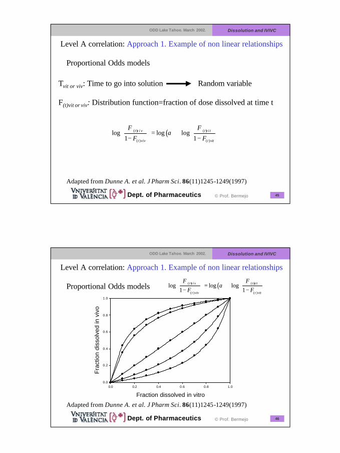
Adapted from Dunne A. et al. J Pharm Sci. 86(11)1245-1249(1997)
( )( ) ( )
( ) ( )
log log log1 1
t v i v t v i t
t viv t vit
F F
F Fα
= + − −
Proportional Odds models
Level A correlation: Approach 1. Example of non linear relationships
Tvit or viv: Time to go into solution Random variable
F(t)vit or viv: Distribution function=fraction of dose dissolved at time t
ODD Lake Tahoe. March 2002. Dissolution and IVIVC
46© Prof. BermejoDept. of Pharmaceutics
Fraction dissolved in vitro0.0 0.2 0.4 0.6 0.8 1.0
Fra
ctio
n di
ssol
ved
in v
ivo
0.0
0.2
0.4
0.6
0.8
1.0
Adapted from Dunne A. et al. J Pharm Sci. 86(11)1245-1249(1997)
( )( ) ( )
( ) ( )
log log log1 1
t v i v tvit
t viv t vit
F FF F
α
= + − − Proportional Odds models
Level A correlation: Approach 1. Example of non linear relationships

24
ODD Lake Tahoe. March 2002. Dissolution and IVIVC
47© Prof. BermejoDept. of Pharmaceutics
Autonomic vs non autonomic relationships
Time
0 5 10 15 20 25 30
X in
vitr
o re
leas
e
0.0
0.2
0.4
0.6
0.8
1.0
1.2
Time0 5 10 15 20 25 30
X in
viv
o re
leas
e
0.0
0.2
0.4
0.6
0.8
1.0
1.2
X (in vitro release)
0 5 10 15 20 25 30
Y (
in v
ivo
rele
ase)
0.2
0.4
0.6
0.8
1.0
ODD Lake Tahoe. March 2002. Dissolution and IVIVC
48© Prof. BermejoDept. of Pharmaceutics
Biorelevant Dissolution Media: Approach 2
qs 1 liter
qs pH 6.8
0.22M
0.029 mM
1.5 mM
5 mM
280-310±10
6.8
Qs 1 literDeionized Waterqs 1 literDeionized Water
Qs pH 5.0NaOHqs pH 6.5NaOH
15.2 gKCl7.7 gKCl
8.65 gAcetic Acid3.9 gKH2PO4
3.75 mMLecithin0.75 mMLecithin
15 mMNa Taurocholate3 mMNa Taurocholate
635±10 Osmolality(mOsmol)
270±10 Osmolality(mOsmol)
5.0pH6.5pH
Fed State simulated intestinal FluidFasted State simulated intestinal Fluids
•From Galia E et al . Pharm Res 15(5) 698-705 (1998)•From Dressman J et al. Pharm Res 15(1) 11-22 (1998)

25
ODD Lake Tahoe. March 2002. Dissolution and IVIVC
49© Prof. BermejoDept. of Pharmaceutics
ClearSightlycloudy
Pearlescent w/TG; Cloudy without TG
Pearlescent at pH 5; Clear at pH 7.5
ClearVisual description56.555 to 7.55 to7.5pH
204103---KCl
--8585142NaCl
--32.40.75Lysolecithin
3.750.7530.60.25Lecithin
--70--Sesame oil
--103-Monocaprin
--20100.25Dodecanoic Acid
144----CH3COOH
-29---KH2PO4
153---Taurocholate
--10105Taurodeoxycholate
FeSSIFFaSSIFFeSIESFESIMSFaSIMSComponent
Concentration (mM)
Adapted from Luner P. and Vander Kamp D. et al. J. Pharm Sci 90(3) 348-359(2001)
ODD Lake Tahoe. March 2002. Dissolution and IVIVC
50© Prof. BermejoDept. of Pharmaceutics
Biorelevant Dissolution Media: Approach 2
qs 1 literDistilled Water
2 gNaCl
2.5 g Na Lauryl sulfate
0.01-0.05 N6.5HCl
Fasted State simulated Gastric Fluid
From Dressman J et al. Pharm Res 15(1) 11-22 (1998)
26
ODD Lake Tahoe. March 2002. Dissolution and IVIVC
51© Prof. BermejoDept. of Pharmaceutics
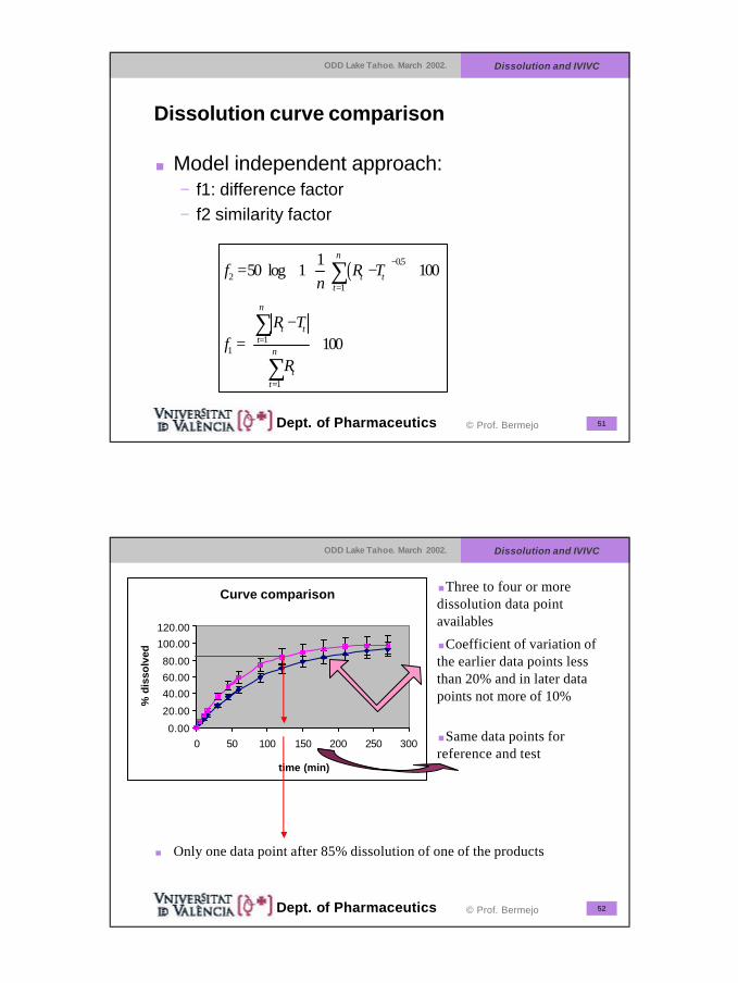
Dissolution curve comparison
< Model independent approach:− f1: difference factor− f2 similarity factor
( ) 0.5
21
11
1
150 log 1 100
100
n
t tt
n
t tt
n
tt
f R Tn
R Tf
R
−
=
=
=
= ⋅ + ⋅ − ⋅
− = ⋅
∑
∑
∑
ODD Lake Tahoe. March 2002. Dissolution and IVIVC
52© Prof. BermejoDept. of Pharmaceutics
< Only one data point after 85% dissolution of one of the products
Curve comparison
0.00
20.00
40.00
60.00
80.00
100.00
120.00
0 50 100 150 200 250 300
time (min)
% d
isso
lved
<Three to four or more dissolution data point availables
<Coefficient of variation of the earlier data points less than 20% and in later data points not more of 10%
<Same data points for reference and test

27
ODD Lake Tahoe. March 2002. Dissolution and IVIVC
53© Prof. BermejoDept. of Pharmaceutics
< A f2 value =50 ensures sameness of the two curves. (An average difference between two profiles of 10% at all sampling data points corresponds to an f2 value of 50)
Average difference %
f2
10
100
50
ODD Lake Tahoe. March 2002. Dissolution and IVIVC
54© Prof. BermejoDept. of Pharmaceutics
< Model dependent approach. − Select the most appropriate model for the dissolution
profiles from the reference batches.− A similarity region is set based on variation of
parameters of the fitted model from the reference batches.
− Calculate the MSD in model parameters between test and reference batches.
− Estimate the 90% confidence region of the true difference between the two batches.
− Compare the limits of the confidence region with the similarity region.
Dissolution curve comparison

28
ODD Lake Tahoe. March 2002. Dissolution and IVIVC
55© Prof. BermejoDept. of Pharmaceutics
Reference batches
Par21n
Par212
Par211
Par 1
Par 1 1n
…
Par 1 12
Par111
Par1
…………
Par 2 2nUnit 2 nPar 1 2nUnit 1 n
Par 2 22Unit 2 2Par 1 22Unit 1 2
Average± SD
Par 2 21Unit 2 1Par121Unit 1 1
Par2Batch2Par2Batch1
Pooled SD=Sqrt((var 1+var2/2)+var(interbatch))Construct similarity region
Difference in Par 1
Dif
fere
nce
in P
ar 2
00
1 std region
2 std region2 std region
ODD Lake Tahoe. March 2002. Dissolution and IVIVC
56© Prof. BermejoDept. of Pharmaceutics
Par21n
Par212
Par211
Par 1
Par 1 1n
…
Par 1 12
Par111
Par1
…………
Par 2 2nUnit 2 nPar 1 2nUnit 1 n
Par 2 22Unit 2 2Par 1 22Unit 1 2
Average± SD
Par 2 21Unit 2 1Par121Unit 1 1
Par2BatchRefPar2BatchTest

29
ODD Lake Tahoe. March 2002. Dissolution and IVIVC
57© Prof. BermejoDept. of Pharmaceutics
( ) ( )
( ) ( ){ }
2 1
2 2
1
( , 1 2 1,0.90)
1 2 1 1 2( 1 2 2) 1 2
( ) ( )
tT R pooled T R
tT R pooled T R
P N N P
D X X S X X
T K D
N N P N NK
N N P N N P
CR K Y X X S Y X X
CR F
−
−
+ − −
= − ⋅ ⋅ − = ⋅
+ − − ⋅ = ⋅ + − ⋅ + −
= ⋅ − − ⋅ ⋅ − − ≤
D2= squared Mahalanobis distance (M)T2=Scaled M distance (Hotelling T2)K= scaling factorNn=number units of lot nP= number of parametersCR= confidence regionXn= vectors of mean parameters of test and ref.S-1pooled=inverse of pooled sample variance-covariance matrix
ODD Lake Tahoe. March 2002. Dissolution and IVIVC
58© Prof. BermejoDept. of Pharmaceutics
Difference in Par 1
Dif
fere
nce
in P
ar 2
0
0
1 std region
2 std region2 std region
90%Confidence region
Contrast CR with similarity region