DISSIPATIVE DYNAMICAL SYSTEMS - Home pages of ESAT

DISSIPATIVE DYNAMICAL SYSTEMS

Jan C. Willems

ESAT-SCD (SISTA), University of Leuven, Belgium

SICE Conference on Control Systems, Kobe, Japan May 28, 2003

THEME

A dissipative system absorbs ‘supply’ (e.g., energy).

How do we formalize this?

Involves the storage function.

How is it constructed? Is it unique?

� KYP, LMI’s, ARE’s.

Where is this notion applied in systems and control?

OUTLINE

1. Lyapunov theory

2. !! Dissipative systems !!

3. Physical examples

4. Construction of the storage function

5. LQ theory � LMI’s, etc.

6. Applications in systems and control

7. Dissipativity for behavioral systems

8. Polynomial matrix factorization

9. Recapitulation

LYAPUNOV THEORY

LYAPUNOV FUNCTIONS

Consider the classical ‘dynamical system’, the flow

��

with � � ��

, the state space,

��

. Denote the set ofsolutions ��

by

�

, the ‘behavior’. The function

�� is said to be a

��

��Lyapunov function for

�if along � � �

��

Equivalent to

� � � � � � � � ��

Typical Lyapunov ‘theorem’:V

X

� � � �� and

� � � �� ! �

for

� "� � � �

#

$ � � � � there holds � % � �

for % � & ‘global stability’

Refinements: LaSalle’s invariance principle.

Converse: Kurzweil’s thm.

LQ theory

for

''% �� ( � � � � � � )+* � � � � � � � � )+, �

� ( )* - * (� ,

(Matrix) ‘Lyapunov equation’

A linear system is (asymptotically) stable iff it has a quadratic positivedefinite Lyapunov function. /

sol’n

* � * )� �� , � , )! �

.

Basis for most stability results in control, physics, adaptation,even numerical analysis, system identification.

Lyapunov functions play a remarkably central role in the field.

Aleksandr Mikhailovich Lyapunov (1857-1918)

Studied mechanics, differential equations.Introduced Lyapunov’s ‘second method’ in his Ph.D. thesis (1899).

DISSIPATIVE SYSTEMS

A much more appropriate starting point for the study of dynamicsare ‘open’ systems. �

0

132154

62687

INPUT/STATE/OUTPUT SYSTEMS

Consider the ‘dynamical system’

�� 9 � :� ; � � 9 =<

9 � >� ? � : � @� A � � � ��

: the input, output, state.Behavior

� � all sol’ns

9� :� � � � > B @ B �<

Let C� > B @ �

be a function, called the supply rate.

C 9� :

models something like the power delivered to the system whenthe input value is 9 and output value is :.

supply

input

output

SYSTEM

DISSIPATIVITY

�

is said to be

��

��dissipative w.r.t. the supply rate C if

/

��

called the

��

��storage function, such that

�� C 9 � � : �

along input/output/state trajectories (

$ 9 �� : ��

.

This inequality is called the dissipation inequality.

Equivalent to

� � � � � 9 � � � � � � � � � 9 � C 9� ; � � 9

for all

9� � � > B �

.

If equality holds: ‘conservative’ system.

Dissipativity� . Increase in storage

�

Supply.

SUPPLY

DISSIPATION

STORAGE

PSfrag replacements

Special case: ‘closed system’: � C� �

then

dissipativity D �

is a Lyapunov function.

Dissipativity is a natural generalization of Lyapunov theory to opensystems.

Stability for closed systems E Dissipativity for open systems.

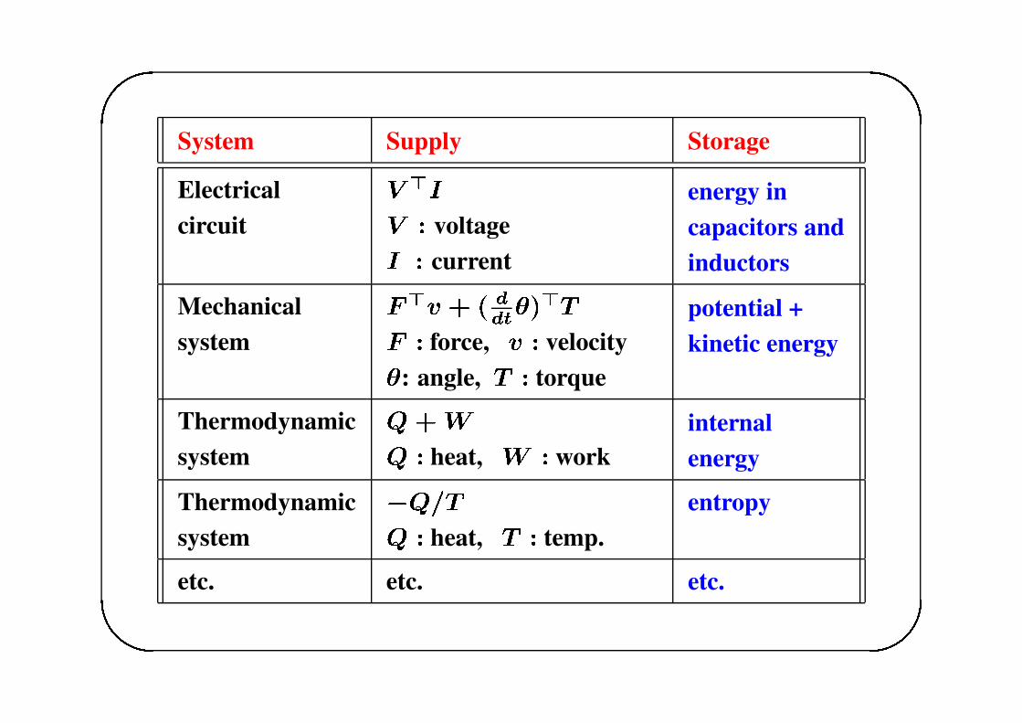
PHYSICAL EXAMPLES

Electrical circuit:

(potential, current)

Dissipative w.r.t.

� FHGJI K � G L G (electrical power).

System Supply Storage

Electricalcircuit

� ) L�� voltageL � current

energy incapacitors andinductors

etc. etc. etc.

Mechanical device:

(position, force, angle, torque)

Dissipative w.r.t. � FHGJI K �� M G )ON G - �� P G )RQ G

(mechanical power)


Electricalcircuit



Mechanicalsystem

N )TS - �� P )Q

N � force, S � velocityP

: angle,

Q � torque

potential +kinetic energy

etc. etc. etc.

Thermodynamic system:

(work)

(heatflow, temperature)

Conservative w.r.t.� FHGI K U G - � F VGJI K W G �

Dissipative w.r.t. X � FHGI KU G

Q Y <


Electricalcircuit



Mechanicalsystem

N )ZS - �� P )Q

N � force, S � velocityP

: angle,

Q � torque

potential +kinetic energy

Thermodynamicsystem

U - W

U� heat,W� work

internalenergy

Thermodynamicsystem

X U [QU� heat,Q � temp.

entropy

etc. etc. etc.

THE CONSTRUCTION OF STORAGE FUNCTIONS

Central question:

Given (a representation of )

�

, the dynamics, and given C,the supply rate, is the system dissipative w.r.t. C, i.e., does there exist

a storage function

�

such that the dissipation inequality holds?

supply

input

output

SYSTEM

Assume known dynamics,Given the system history, how much ‘energy’ is stored?

Assume henceforth that a number of (reasonable) conditions hold:

� �� ; �� C ��

;Maps and functions (including

�

) smooth;State space

�

of

�

‘connected’:every state reachable from every other state;

Observability.

‘Thm’: Let

�

and C be given.

Then

�

is dissipative w.r.t. C iff

C 9 �� : �� '% \ �

for all periodic

9 � � : � � � � � �

.

The AVAILABLE STORAGE and the REQUIRED SUPPLY

Two universal storage functions:

1. The available storage

�^]_ ] `a ] b adc �fe � �

ghi jJk jml npo q jl npo r jl n ns to r je n I ru o r jJv n I e w Xx v

e C 9 � � : � '% y

2. The required supply

�{zc| } ` zc ~ �fe � �

�� jJk jl n o q jl npo r jl n n s to r j�� v n I e o r je n I ru w e� v

C 9 �� : �� '% y

supply

input

output

SYSTEM

!! Maximize the supply extracted, starting in fixed initial state� available storage.

supply

input

output

SYSTEM

!! Minimize the supply needed to set up a fixed initial state� required supply.

Storage f’ns form convex set, every storage function satisfies

�^]_ ] ` a ] b adc � �� {zc| } ` zc ~<

LINEAR SYSTEMS with QUADRATIC SUPPLY RATES

Assume

�

linear, time-invariant, finite-dimensional:

�� ( � - � 9� :� � � �

and C quadratic: e.g.,

C� 9� : �� 9 � � � X � � : � � �<E.g., for circuits 9� � x �� :� �� , etc.

Assume

(� �

controllable, (� � observable.� C � � � - � L C X ( � K �

, the transfer function of

�

.

Theorem: The following are equivalent:

1.

�

is dissipative w.r.t. C (i.e., there exists a storage function

�

),

2.

$ 9 � � : � � � � � �� ,� � 9 � � �p�5� \ � � : �� p�5� ,

3.

� � � ��

for all� �

,

4.

/

a quadratic storage f’n,� � � � )O� � � � � � )

,

5. there exists a solution

� � � )

to theLinear Matrix Inequality (LMI)�

�( )� - � ( - � ) � � �

� )R� X L�

� � ��6. there exists a solution

� � � )

to theAlgebraic Riccati Inequality (ARIneq)

( )� - � ( - � � � ) � - � ) ��

7. there exists a solution

� � � )to the Algebraic Riccati Equation

(ARE) ( )� - � ( - � � � ) � - � ) �� <

Solution set (of LMI, ARineq) is convex, compact, and attainsits infimum and its supremum:� � � � � � x

These extreme sol’ns

� � and

� x

corresponding to the availablestorage and the required supply, themselves satisfy the ARE.

Extensive theory, relation with other system representations,many applications, well-understood (also algorithmically).

Connection with optimal LQ control, semi-definite programming,

�v

control, etc.

Important refinement: Existence of a

� \ �

(i.e., bounded from below)

�e

� vC 9 �� : �� '% \ �<

In LQ case .

� � e� v � � 9 � � � � '% \ � e� v � � : �� '% �

� g hi �J s ¡ ¢£ c j n¤ e ¥ � � � C � � � � � � � � ��¦ § � �,

Note def. of

�v -norm !

� /

sol’n

� � � ) \ �

to LMI, ARineq, ARE.

� KYP-lemma.

APPLICATIONS

� Synthesis of RLC-circuits

� Robust stability(‘the interconnection of dissipative systems is stable’)

� Stabilization (by ‘passivation’)

� Robust stabilization (by making the loop dissipative),�v -control

� Norm estimation (e.g., bounding the balanced reduction error)

� Covariance generation

� � � �

Dissipative systems (and LMI’s which emerged from this) play aremarkably central role in the field.

BEHAVIORAL SYSTEMS

The input/output, nor input/state/output approach are not logicalstarting points for studying

� (open) physical systems

� interconnected systems

� dissipative systems

� � � �

� ‘behavioral systems’

(potential, current)

(position, force, angle, torque)

(work)

(heatflow, temperature)

BEHAVIORAL SYSTEMS

A dynamical system =

� � ¨ � ©� �

¨ ª

, the time-axis (= the relevant time instances),

©

, the signal space (= where the variables take on their values),

� ª © «

: the behavior (= the admissible trajectories).

� � ¨ � ©� �

For a trajectory ¬� ¨ � ©� we thus have:

¬ � �

: the model allows the trajectory ¬ �

¬ [ � �

: the model forbids the trajectory ¬<

N

3

2

1

Today:

¯® °²±³® °´ ±µ ® sol’s of system of linear constant coefficient ODE’s.

DIFFERENTIAL SYSTEMS

Consider ¶e ¬ - ¶ K'

'% ¬ - � � � - ¶ �' �

'% � ¬� ��with

¶e � ¶ K � � � � � ¶ � � � ·¸ <

Combined with the polynomial matrix

¶ ¹ � ¶e - ¶ K ¹ - � � � - ¶ � ¹ � �

we obtain the short notation

¶ ''% ¬ � �<

¶ ''% ¬ � �<

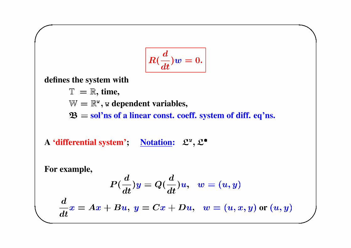
defines the system with¨ � � time,©� ¸ � º dependent variables,� � sol’ns of a linear const. coeff. system of diff. eq’ns.

A ‘differential system’; Notation:

»¸ � » �

For example,

¼ ''% :� U ''% 9� ¬� 9� :

''% �� ( � - � 9� :� � � - � 9� ¬� 9� � � :

or

9� :

CONTROLLABILITY

Controllability .

system trajectories must be ‘patch-able’, ‘concatenable’.

w

1

w

w

w

w

2

1

0

2

T0

time

W

time

W W

Is the system defined by

¶e ¬ - ¶ K'

'% ¬ - � � � - ¶ �' �

'% � ¬� ��with ¬ � ¬ K � ¬ � � � � � � ¬¸

and

¶e � ¶ K � � � � � ¶ � � � ·¸ �

i.e.,

¶ ''% ¬ � ��

controllable?

We are looking for conditions on the polynomial matrix

¶

and algorithms in the coefficient matrices

¶e � ¶ K � � � � � ¶ � .

Thm: The following are equivalent:

1.

¶ �� ¬� �

defines a controllable system

2. ½ ¾� ¿ ¶ À

is independent of

À

for

À � Á.

Example: Â K ''% ¬ K � Â � ''% ¬ � ¬ K � ¬ � scalar)

is controllable if and only if Â K and Â � have no common factor.

Representations of

» �

:

¶ �� ¬ � �

called a ‘kernel’ representation of

� � ¿�Ã ½ ¶ �� Another representation: ¬ � Ä �� Ycalled an ‘image’ representation of

� � ��Å Ä �� =<

Elimination theorem # every image is also a kernel.

¿¿ Which kernels are also images ??

Theorem: The following are equivalent for

� � » � �1.

�

is controllable

2.

�

admits an image representation

3. � � �

QDF’s

The quadratic map acting on ¬� � ¸

and its derivatives, definedby

¬� � Æo G ' Æ' � Æ ¬ )ÈÇ Æo G ' G' � G ¬

is called quadratic differential form (QDF).Ç Æo G � ¸ ·¸ÈÉ WLOG:

Ç Æo G� Ç )Go Æ .

Introduce the

Ê

-variable polynomial matrixÇ

Ç Ë � Ì �Æo G

Ç Æo GË Æ Ì G<

Denote the QDF as

UÎÍ . QDF’s are parametrized by

¸ ·¸ ÏË � Ì Ð <

DISSIPATIVE BEHAVIORAL SYSTEMS

We consider only controllable linear differential systemsand QDF’s for supply rates.E.g.,

� ) L

for electrical circuits,

N ) �� M for mechanical systems, ...

Definition:

� � » �

, controllable, is said to be dissipativewith respect to the supply rate

UÑÍ (a QDF) if

�ÓÒ UÎÍ ¬ '% \ �

for all ¬ � �

of compact support.

In any trajectory from rest back to rest, supply is absorbed.

STORAGE FUNCTION

Dissipativity� . �Ò UÑÍ ¬ '% \ �

for ¬ � �

compact supp<Can this be reinterpreted as: As the system evolves,

some supply is stored, some is dissipated?

!! Invent storage, such that:

�� Storage

�

Supply.SUPPLY

DISSIPATION

STORAGE

PSfrag replacements

MAIN RESULT

Theorem: Let

� � » �

be controllable, and

U Í be a QDF. Then

ÒUÎÍ ¬ '% \ �

for all ¬ � �

of compact support

if and only if

there exists a QDF,

UÑÔ , the storage function such that

�� UÔ ¬ % � UÑÍ ¬ %

for all ¬ � �

and % � <Note: The computation of

Õis an LMI involving

¶

(or

Ä

) and

Ç

!

OUTLINE of the PROOF

Using controllability and the existence of an image representation,reduce to case that ¬ is ‘free’.

Now consider, for a given (smooth) ¬� � ¸,

infimum

e� v

UÑÍ Ö ¬ '% �

with infimum taken over all

Ö ¬ � �such that

Ö ¬ % � ¬ %

for % \ �

.� the ‘available storage’.

Prove that this infimum is a QDF,

U Ô ¬ �

, and that it qualifies as astorage function.

This proof provides (but does not rely on!) a simple proof of thefollowing (known) factorization result for polynomial matrices.Consider

* ) ¹ * ¹ � , ¹

,

is a given real polynomial matrix;

*

is the unknown.

For

, � Ï¹ Ð

, a scalar, this eq’n is solvable (for* � � Ï¹ Ð

) iff

, �× \ �

for all × � <

For

, � � · � Ï¹ Ð

, it is solvable (with* � � · � Ï¹ Ð

!) iff

, �× � , ) × \ �

for all × � <

Btw: For multivariable polynomials, and under the obvious symmetryand positivity requirement,

, �× � , ) × \ �

for all × � � �this equation can nevertheless in general not be solved over thepolynomial matrices, for

* � � · � Ï¹ Ð

, but it can be solved over thematrices of rational functions, i.e., for

* � � · � ¹ .

This is Hilbert’s 17-th pbm!

Remarks

� Very important refinement:� e� v UÎÍ ¬ '% \ � . / Õ

such that

UÎÔ ¬ \ �.

� The storage function is always a state function.Not so for discrete-time systems (Kaneko).

� Generalized to systems describes by PDE’s. Uses factorizability formultivariable polynomials. Constructs stored energy and flux (the‘Poynting vector’) for Maxwell’s eq’ns.

Ø Applies to

Ù{Ú problem in behavioral setting, with the famous‘coupling condition’ of two storage functions.

The notion of a dissipative system:

� Generalization of ‘Lyapunov function’ to open systems

� Central concept in control theory: many applications to feedbackstability, stabilization, robust (

� v -) control, adaptive control,system identification, passivation control

� Stimulated emergence of LMI’s, semi-definite programming

� Other applications: system norm estimates, passive electricalcircuit synthesis procedures, covariance generation

� Combined with behavioral systems, dissipativity forms a naturalsystems concept for the analysis of open physical systems

� Notable special case: second law of thermodynamics

� Forms a tread through modern system theory

More info, copy sheets? Surf tohttp://www.esat.kuleuven.ac.be/ Ûjwillems

Thank you !

DISSIPATIVE DYNAMICAL SYSTEMS - Home pages of ESAT

Documents

Transcript of DISSIPATIVE DYNAMICAL SYSTEMS - Home pages of ESAT