Dissertations of the Institute of Geography and Regional Development University of Wrocław 12

MACIEJ KRYZA 1)

MAREK BŁAŚ 1)

ANTHONY JAMES DORE 2)

MIECZYSŁAW SOBIK 1)

1) University of Wrocław, Institute of Geography and Regional Development,

Pl. Uniwersytecki 1, 50-137 Wrocław, Poland.

2) Centre for Ecology and Hydrology, Bush Estate, Penicuik, Midlothian EH26 OQB,

United Kingdom.

MODELLING THE CONCENTRATION AND DEPOSITION OF AIR POLLUTANTS IN POLAND WITH THE FRAME MODEL

Wrocław, 2009

Institute of Geography and Regional Development

University of Wrocław

Reviewers:

Prof. Jacek Namieśnik (Gdańsk University of Technology, Chemical Faculty)

Dr hab. inż. Wojciech Mill (Institute of Environmental Protection, Section of Integrated Modelling)

Editorial Board of the Series

Dr hab. Zdzisław Jary

(University of Wrocław, Institute of Geography and Regional Development)

The volume has been published with the financial support of

The Ministry of Science and Higher Education

Cover figures: Emission (at the back), concentration (in the middle) and deposition (on top) nitrogen oxides in year 2002 in Poland.

Copyright by Maciej Kryza, Marek Błaś, Anthony J. Dore and Mieczysław Sobik 2009

ISBN 978-83-928193-7-0

Abbreviations: AENEID – Atmospheric Emission for National Environmental Impacts Determination

AirBase – European Air quality data base

ATMs – Atmospheric Transport Models

CBED – Concentration Based Estimated Deposition

CIEP – Chief Inspectorate for Environment Protection

CL – Critical Load

CLev – Critical Level

CLRTAP – Convention on Long Range Transport of Air Pollutants

CORINAIR – Core Inventory of Air Emission

CORINE – Coordination of Information on the Environment

DAMOS – Danish Ammonia Modelling system

EMEP – European Monitoring and Evaluation Programme

EMEP4UK – EMEP model applied with increased spatial resolution over the British Islands

EPER – European Pollutant Emission Register

FRAME – Fine Resolution Atmospheric Multi-pollutant Exchange

FRAME-PL – FRAME model with domain covering Poland

FRAME-UK – FRAME model with domain covering the United Kingdom

FRAME-Europe – FRAME model with domain covering Europe

GIS – Geographical Information System

GRASS – Geographic Resources Analysis Support System

HARM – Hull Acid Rain Model

HIRLAM – High-Resolution Limited Area Model

IEP – Institute of Environmental Protection

IMGW – Institute of Meteorology and Water Management

LRTAP – Long-range Transboundary Air Pollution

LTP – Long Term Precipitation

LWC – Liquid Water Content

NAEI – National Atmospheric Emission Inventory

NARSES – National Ammonia Reduction and Strategies Evaluation System

NEC – National Emission Ceilings

OPS – Operational Priority Substance Model

SAI – Surface Area Index

SFE – Seeder-feeder effect

SNAP – Selected Nomenclature for sources of Air Pollution

STOCHEM – Global 3-D Lagrangian tropospheric chemistry model

TERN – Transport over Europe of Reduced Nitrogen

TIC - Total Inorganic Ionic Content

TRACK – TRajectory model with Atmospheric Chemical Kinetics

UBA – The Federal Environment Agency of Germany (UmweltBundesAmt)

UNECE – United Nations Economic Commission for Europe

WMO – World Meteorological Organization

CONTENTS:

1. AIR POLLUTION IN POLAND 7

1.1. The European context 7

1.2. Unified EMEP model – background for national scale analyses in Poland 7

1.3. Emission of sulphur and nitrogen compounds in Poland 9

1.4. Emission abatements in Poland 12

1.5. Summary 14

1.6. References 14

2. INTRODUCTION TO ATMOSPHERIC MODELLING 17

References 18

3. FRAME MODEL DESCRIPTION 21

3.1. FRAME model domain 21

3.2. Emission 22

3.3. Plume rise 22

3.4. Diffusion 23

3.5. Chemistry 24

3.6. Dry deposition 25

3.7. Wet deposition 25

3.8. Diurnal cycle 26

3.9. Wind frequency and wind speed rose 26

3.10. Computational performance 26

3.11. References 27

4. INPUT DATA FOR FRAME-PL MODEL 29

4.1. Meteorological data 29

4.1.1. Radiosonde wind data 29 4.1.2. Rainfall data 31 4.1.3. The seeder-feeder effect 33

4.2. Emission inventory 35

4.2.1. Introduction 35 4.2.2. Input data and methods 35 4.2.3. Area emission - results and validation 39

4.3. Summary 42

4.4. References 43

5. FRAME MODEL RESULTS – CONCENTRATION AND DEPOSITION OF AIR POLLUTANTS IN POLAND 45

References 55

6. EVALUATION OF THE FRAME MODEL RESULTS 57

6.1. Data and methods 57

6.1.1. Measurement data 57 6.1.2. Comparison with the EMEP-Unified model 58

6.2. Model evaluation results 59

6.2.1. Air concentration 59 6.2.2. Wet deposition 60

6.3. Comparison with the EMEP model results 63

6.4. Deposition budget 64

6.5. Summary and conclusions 68

6.6. References 68

7. APPLICATIONS OF THE FRAME MODEL 71

7.1. The influence of the low-level orographic clouds on the spatial distribution of wet deposition in Poland 71

7.2. Exceedances of critical loads and levels 73

7.2.1. Introduction 73 7.2.2. Exceedance estimates 74 7.2.3. Results 74

7.3. Source-receptor analysis 76

7.4. References 78

8. FACTORS CONTROLLING DEPOSITION PROCESSES IN DIFFERENT SCALES 81

8.1. Atmospheric circulation – the role of the meso-scale conditions on air pollutants concentration and deposition 81

8.2. Topo–climatic factors and air pollutants concentration and deposition 81

8.3. Microscale factors and air pollutants concentration and deposition 82

8.4. References 83

9. NON PRECIPITATION ATMOSPHERIC DEPOSITS 85

9.1. Introduction 85

9.2. Meteorological interpretation 85

9.2.1. Fog deposition 85 9.2.2. Dew and hoarfrost 86

9.3. Total ionic content of hydrometeors 86

9.4. The role of hydrometeors in wet deposition budget 88

9.5. Deposition hot spots in the Sudety Mts. 89

9.6. References 90

1. AIR POLLUTION IN POLAND 1.1. THE EUROPEAN CONTEXT

Pollutant deposition became an issue of international interest in the 1950s and 1960s, when a relationship was found between sulphur emission in continental Europe and acidification of Scandinavian lakes. Power plants usually emit pollutants from high stacks so that the pollutants are not easily washed down to the surface nearby, but are subjected to the long-range transport. The wind can transport pollutants over long distances, sometimes hundreds to thousands of kilometres (Jacobson, 2002). Therefore environmental effect of air pollutants deposition is often a regional, long-range as well as transboundary problem, when atmospheric pollutants are transported across political boundaries.

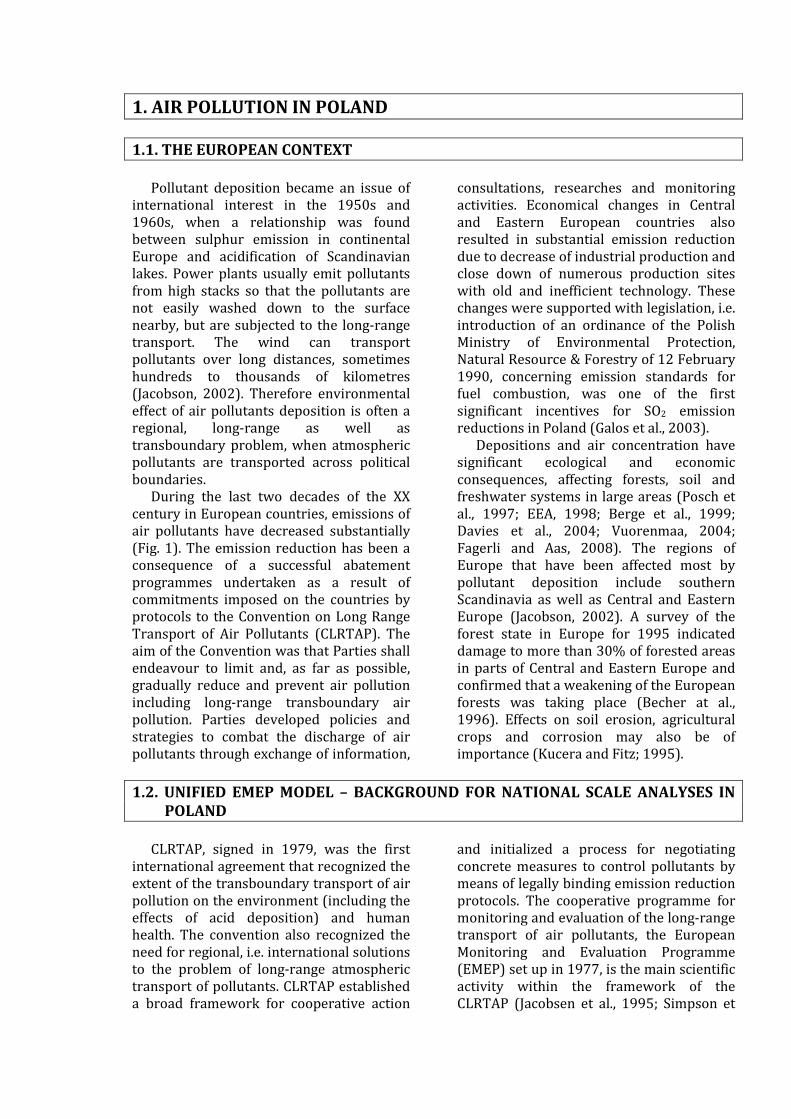
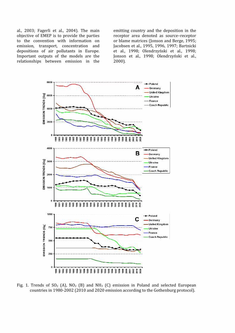
During the last two decades of the XX century in European countries, emissions of air pollutants have decreased substantially (Fig. 1). The emission reduction has been a consequence of a successful abatement programmes undertaken as a result of commitments imposed on the countries by protocols to the Convention on Long Range Transport of Air Pollutants (CLRTAP). The aim of the Convention was that Parties shall endeavour to limit and, as far as possible, gradually reduce and prevent air pollution including long-range transboundary air pollution. Parties developed policies and strategies to combat the discharge of air pollutants through exchange of information,

consultations, researches and monitoring activities. Economical changes in Central and Eastern European countries also resulted in substantial emission reduction due to decrease of industrial production and close down of numerous production sites with old and inefficient technology. These changes were supported with legislation, i.e. introduction of an ordinance of the Polish Ministry of Environmental Protection, Natural Resource & Forestry of 12 February 1990, concerning emission standards for fuel combustion, was one of the first significant incentives for SO2 emission reductions in Poland (Galos et al., 2003).

Depositions and air concentration have significant ecological and economic consequences, affecting forests, soil and freshwater systems in large areas (Posch et al., 1997; EEA, 1998; Berge et al., 1999; Davies et al., 2004; Vuorenmaa, 2004; Fagerli and Aas, 2008). The regions of Europe that have been affected most by pollutant deposition include southern Scandinavia as well as Central and Eastern Europe (Jacobson, 2002). A survey of the forest state in Europe for 1995 indicated damage to more than 30% of forested areas in parts of Central and Eastern Europe and confirmed that a weakening of the European forests was taking place (Becher at al., 1996). Effects on soil erosion, agricultural crops and corrosion may also be of importance (Kucera and Fitz; 1995).

1.2. UNIFIED EMEP MODEL – BACKGROUND FOR NATIONAL SCALE ANALYSES IN

POLAND

CLRTAP, signed in 1979, was the first international agreement that recognized the extent of the transboundary transport of air pollution on the environment (including the effects of acid deposition) and human health. The convention also recognized the need for regional, i.e. international solutions to the problem of long-range atmospheric transport of pollutants. CLRTAP established a broad framework for cooperative action

and initialized a process for negotiating concrete measures to control pollutants by means of legally binding emission reduction protocols. The cooperative programme for monitoring and evaluation of the long-range transport of air pollutants, the European Monitoring and Evaluation Programme (EMEP) set up in 1977, is the main scientific activity within the framework of the CLRTAP (Jacobsen et al., 1995; Simpson et

al., 2003; Fagerli et al., 2004). The main objective of EMEP is to provide the parties to the convention with information on emission, transport, concentration and depositions of air pollutants in Europe. Important outputs of the models are the relationships between emission in the

emitting country and the deposition in the receptor area denoted as source–receptor or blame matrices (Jonson and Berge, 1995; Jacobsen et al., 1995, 1996, 1997; Bartnicki et al., 1998; Olendrzyński et al., 1998; Jonson et al., 1998; Olendrzyński et al., 2000).

Fig. 1. Trends of SO2 (A), NO2 (B) and NH3 (C) emission in Poland and selected European

countries in 1980-2002 (2010 and 2020 emission according to the Gothenburg protocol).

The EMEP programme relies on three main elements: (1) collection of emission data; (2) measurements of pollutants in air and precipitation and (3) modelling of atmospheric transport and deposition of air pollutants in Europe. For many countries EMEP calculations are the main source of information on transboundary exchange of pollutants. Through the combination of these three elements the main objectives of EMEP are to: � Provide observational and modelling

data on pollutant concentration, deposition, emission and transboundary fluxes on the regional scale and identify their trends in time;

� Identify the sources of the pollutant concentration and depositions and to assess the effects of emission abatements;

� Improve our understanding of chemical and physical processes relevant to assessing the effects of air pollutants on ecosystems and human health in order to support the development of cost-effective abatement strategies.

Currently used EMEP-Unified model is a Eulerian atmospheric transport model that is driven by real-time meteorology (Simpson et al., 2003; Fagerli et al., 2004). The model is applied over Europe with a a 50 km x 50 km grid and meteorological fields updated every 3 hours (Jacobsen et al., 1995; Simpson et al., 2003; Fagerli et al., 2004). EMEP domain is centered over Europe and also includes most of the North Atlantic and the polar region. The model uses 20 vertical layers to describe the troposphere, with the vertical domain

extending up to 16 km altitude. By setting the emission of pollutant gases (NH3, NOx and SO2) from individual countries to zero, the model generates source-receptor matrices of the contribution to deposition in one country associated with emission from other countries.

Whilst EMEP deposition fields provide a useful guide to the magnitude of pollutant deposition, there is a need for nation states to develop their own national scale models to resolve atmospheric physical and chemical processes which occur at a much finer resolution than that currently available in the EMEP model: � The magnitude of atmospheric

deposition of nitrogen and sulphur in the vicinity of strong sources varies on scales of several km, much finer than the grid resolution of the EMEP model.

� The vertical grid resolution in the lowest layer is 50 m. The implication of this are that chemical species which are emitted at low level (such as NOX from vehicle exhausts and NH3 from agricultural sources) will have their ground level concentration rapidly diluted by mixing into a deep surface layer.

� The influence of the seeder-feeder effect in causing enhanced deposition in upland regions has not currently been incorporated into the EMEP model with 50 km x 50 km resolution.

� Annual precipitation in hill regions is known to vary significantly at a 1 km scale.

Comparison of the results of the EMEP model and the FRAME model for Poland is illustrated in section 5.1.

1.3. EMISSION OF SULPHUR AND NITROGEN COMPOUNDS IN POLAND

Over the last decades, the anthropogenic emission of sulphur and nitrogen has decreased significantly, especially in Europe (Erisman et al., 2003). According to EMEP emission inventory, abatement in SO2 emissions reached 80% over the period 1980 to 2006 (from 25.0 Tg to ca. 5.0 Tg) and 35% if NOx is considered (6.9 Tg in 1980 and 4.5 Tg in 2006, Vestreng et al., 2007).

Since the beginning of the nineties, a substantial reduction in gaseous emission

have been observed in Poland, with SO2 being reduced most significantly (Fig. 1; Abraham et al., 2003). Emission of SO2, which amounted 1131 Gg in 2007, has decreased by about 72% since 1980, and 65% since 1990 (Mitosek et al., 2004; Olendrzyński et al., 2009). The scale of emission abatements was even larger in some neighbouring countries – e.g. the Czech Republic and Germany (87% and 86% respectively). NOx emission dropped by 48% in Poland between 1980 and 2007.The

larger reductions were observed in the Czech Republic and Germany (70% and 62% respectively).

Historically, Poland is in the group of European countries with the largest sulphur and nitrogen emission. This is because coal is the main fuel used in energy production, industry, and in non-industrial combustion (Dębski et al., 2009). In the year 1980, only Germany and United Kingdom had higher SO2 emission (Fig. 1). Since the early 1990’s, sulphur and, to the less extent, nitrogen emission show downward trend in Poland (Vestreng et al., 2007). At the beginning of 1990’s, the abatement can be attributed to the transition from a centrally planned to free-market economy, and the largest abatements are observed in the energy production sector (Mill, 2006). After the mid 1990’s, the energy production starts to increase, while SO2 emission still shows downward trend due to successful implementation of abatement policy, which covers over 50% of installed power capacities in professional power-plants (Galos et al., 2003). These regulations resulted in reduction of sulphur emission in professional power industry from over 750 Gg of S in 1990 to 400 Gg in 2000. Emission of reduced nitrogen in Poland has fallen by 41% since 1985 (Olendrzyński et al., 2004).

The reduction of pollution emission originating especially from the power industry is executed by the introduction of advanced combustion techniques, e.g. flue gases cleaning. To lower SO2 emission from both electric power and district heating plants, fuel with low sulphur contain and new desulfurization equipment were used. The decrease of SO2 emission was achieved by the use of electrostatic precipitators and circulating fluidised bed boilers which can absorb up to 90% of the SO2 that would otherwise go into the atmosphere. Thanks to various improvements SO2 emission from e.g. the Turów Power Plant was reduced by 83% from 1989 levels (Libicki, 1998; Marszalik, 1995). Other methods were applied to reduce NOX emission: denitrifying equipment, low NOx emission burners and employing exhaust-gas recirculation methods. The recent increase of NOx emission can be attributed to the road traffic. Further abatements of nitrogen

oxides emission are one of the major international and national environmental policy targets, and should lead to decrease in acidification and eutrophication of natural ecosystems.

One of the main difference between Poland and other European countries emitting large amounts of sulphur and nitrogen is the contribution of non-industrial combustion plants (Selected Nomenclature for sources of Air Pollution - SNAP sector 02) to total national emission of these pollutants. In Poland, commercial, residential and agriculture combustion (i.e. SNAP sector 02 non-industrial combustion) of hard coal contributes 18% of national total emission of sulphur and 5% of NOx (Fig. 2). Moreover, the emission abatements in SNAP sector 02 do not follow the overall reductions of sulphur and nitrogen emission. The decrease of SNAP sector 02 emission in Poland is very slow, if compared with other European countries that undergone similar economical changes over the recent years, like the Czech Republic, and, more recently, Ukraine. The economical reasons are probably behind that, as the gas fuel is expensive (small domestic resources available, small diversification of import), especially if compared to coal. Moreover, switch from coal to gas in residential combustion is possible only after previous investments in heating facilities, and these costs also have to be considered.

The changes in NH3 emission in Poland are relatively small, if compared to changes in sulphur and oxidised nitrogen emissions (Fig. 1, Mitosek et al., 2004). The largest reductions, in the beginning of 90ties, can be related to economical changes in Poland. While SO2 and NOx emission still show a downward trend, the NH3 emission level has stabilized at about 320 Gg since the year 2000. Predominant source of ammonia emitted in Poland is agriculture (94% of total emission in 2000) with the main role of animal husbandry and, to a smaller extent, the fertilizer application.

According to EMEP blame matrices for year 2007, ca. 37% of sulphur deposited in Poland comes from transboundary transport, while the rest can be attributed to domestic sources. At the same time, considerable amount of oxidized sulphur

emitted in Poland is transported across the borders and deposited in other countries (over 35% of total emission). As can be seen from the EMEP calculations, for many years Poland has held the position of a net-exporter (the country with export of the sulphur and nitrogen compounds is larger

than their import). The largest amounts of sulphur and nitrogen compounds imported to Poland in 2007 come from Germany (6%) and Czech Republic (5%). The pollutants exported from Poland were transmitted mainly to Russia, Ukraine and Belarus and to the Scandinavian countries.

Fig. 2. Trend in emission of SO2 (A) and NOx (B) in Poland according to SNAP sectors (EMEP

emission inventory).

Fig. 3. Long-term pH values of precipitation at Szrenica (1330 m a.sl.) and Śnieżka (1602 m a.s.l.)

sites in the Western Sudety Mts.; average pH derived from H+ concentration and volume weighted.

1.4. EMISSION ABATEMENTS IN POLAND

In the target year 2010 and at the emission ceilings set by the NEC (National Emission Ceilings) Directive (2001/81/UE) the ecological interim target will be achieved on all the territory of Poland except the Upper Silesia region (Mill and Schlama, 2007). The progress of meeting the ecological target is strongly influenced by the transboundary fluxes of sulphur and nitrogen in western and southern regions of Poland. The implementation of the NEC Directive will effect in 80% reduction in areas of exceeded critical loads of acidity to compare with the year 1990.

Critical loads and levels concepts link air pollution deposition and concentration with effects to natural ecosystems. Critical loads of acidity determine the highest tolerable deposition of sulphur and nitrogen and set up a quantitative measure of sensitivity of a given ecosystem to acid deposition, according to the definition formulated by Nilsson and Grennfelt (1988). The total area affected by exceedances of critical loads for acid deposition on a European scale was about 20% in the mid eighties (Posch et al., 1997; Berge et al., 1999). Calculations made by Mill (2006) showed that the area with the critical loads exceeded for acidification gradually increased in Poland in the period 1980-1989. Since 1990 a substantial decline has been observed with a further downward

trend continue until the recent times. In spite of nearly 70% reduction of sulphur emission in the past two decades in Poland the threat of acidification for forest and other natural ecosystems is still relatively high, affecting 40% of forested areas (Mill et all., 2003; Mill, 2006). Such a tendency in forest deterioration is reported by other Central European countries and the possible reason of it is associated with nitrogen deposition and specifically with deposition of ammonia.

Chemical composition of rain and, in particular, cloud water, is a sensitive indicator of changes in air pollutants emission (Ferrier et al., 1995; Minami and Ishizaka, 1996; Acker et al., 1998; Puxbaum and Tscherwenka, 1998; Sobik, 1999; Fišák and Řezáčová, 2001; Collett et al., 2002; Błaś et al., 2008). Changes in annual precipitation volume weighted pH values at Szrenica (UWr. station) and Śnieżka (EMEP station) are shown in Fig. 3. Between the mid eighties and 2004 the acidity of precipitation decreased by factors of 5 to 6 at Snieżka Mt. and by 7 to 8 during the last 15 years at Szrenica. This indicates that the average annual hydrogen concentration in precipitation at Śnieżka decreased from 125 µMoles∙l-1 in 1985 to ca. 25-30 µMoles∙l-1 between 2000-2004 and from 150 to ca. 30-40 µMoles∙l-1 at Szrenica. It should be also

mentioned, that such significant changes with an upward tendency of pH values were observed in other mountainous region in the south-west part of Poland (Mitosek et al., 2004; CIEP, 2007). The decrease in cloud and rain water acidity can be attributed to both European decrease in sulphur and nitrogen emission, as well as abatements in local sources (e.g. like Turów Power Plant in case of the Szrenica and Śnieżka monitoring stations).

In Poland, only one monitoring station with long-term, continuous cloud chemical measurements exists. At the Mt. Szrenica in the Western Sudety Mts., cloud water samples have been collected daily since 1989. The largest relative decrease (percentage of a given ion in Total Inorganic Ionic Content – TIC) occurred in the case of sulphates (from 29% in the warm season in

1995 to ca. 10% in 2004) and the H+ cation (from 13% to 8%). Nitrates and ammonium became the dominant ions in 2004 with an increase of relative concentration from 17 to 28% and from 22 to 26%, respectively. These changes resulted in a spectacular decrease of acidity, expressed by an increase of over half a unit in pH values (from 3.8 in 1990 to 4.5 in 2004; Błaś et al., 2008).

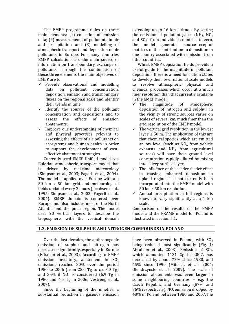
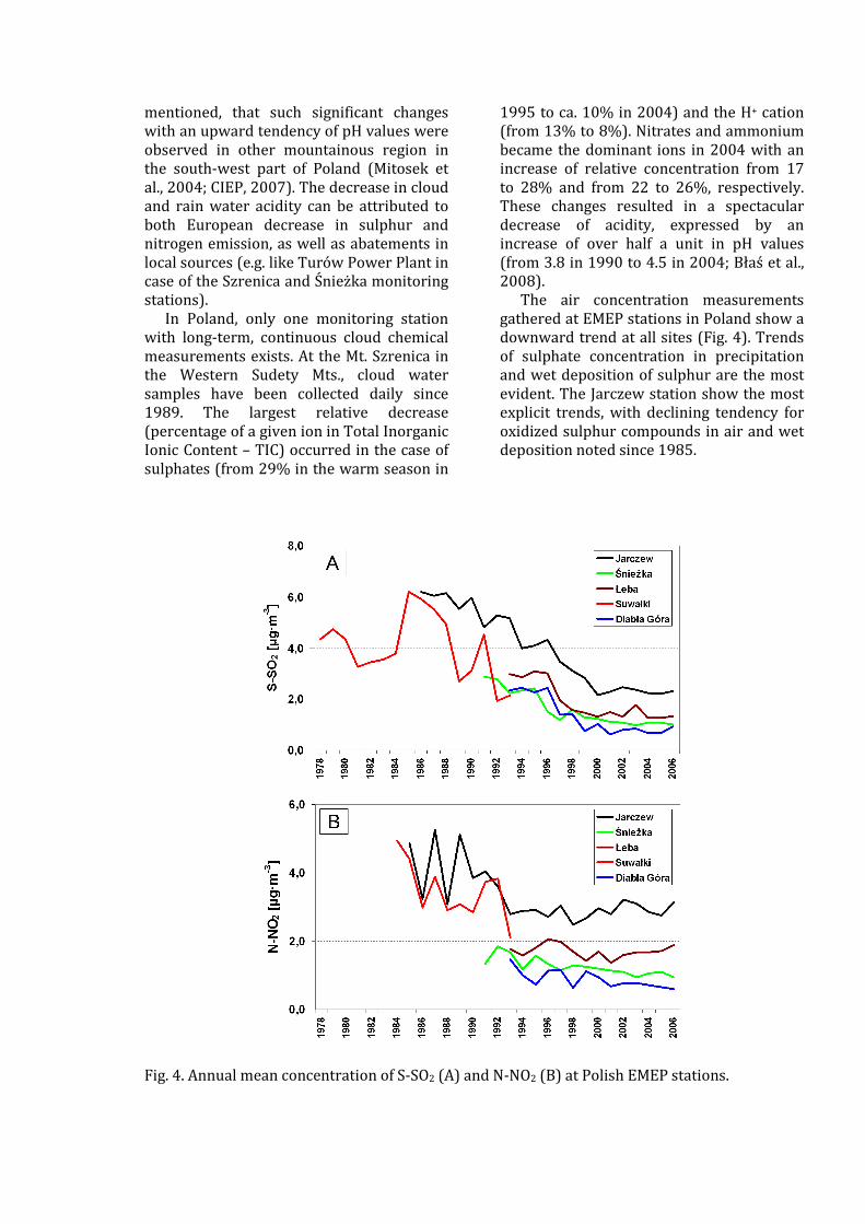
The air concentration measurements gathered at EMEP stations in Poland show a downward trend at all sites (Fig. 4). Trends of sulphate concentration in precipitation and wet deposition of sulphur are the most evident. The Jarczew station show the most explicit trends, with declining tendency for oxidized sulphur compounds in air and wet deposition noted since 1985.

Fig. 4. Annual mean concentration of S-SO2 (A) and N-NO2 (B) at Polish EMEP stations.

1.5. SUMMARY

A substantial reduction of air pollutant emission over the past two decades has resulted in general improvement of air quality in Poland. Dynamics of the observed changes in air pollution concentration is however different for various pollutants and areas. The largest reductions in air concentration occurred for SO2 - both in urban and rural areas. The areas with the highest air concentration noted in the past show the largest improvements (Upper Silesia and the Black Triangle region). The downward trend in NO2 emission in Poland is less pronounced than for SO2. Changes in air concentration of NO2 in ambient air over

the years are also smaller, if compared with SO2. However, in comparison with the eighties, an improvement in air quality with regard to NO2 is also significant.

Emission abatements, both from European and domestic sources caused large environmental benefits and resulted in decrease of areas with exceeded critical loads and levels. However, the total area of critical loads exceeded in Poland is still significant. As in rest of European countries, there is also change in relative contribution of chemical species to acidification and eutrohpication, with reduced nitrogen gaining in importance.

1.6. REFERENCES

Abraham, J., Berger, F., Ciechanowicz-Kusztal, R., Jodłowska-Opyd, G., Kallweit, D., Keder, J., Kulaszka, W., Novák, J., 2003, Common report on air quality in the Black Triangle Reg. 2002. ČHMÚ, WIOŚ, LfUG and UBA Press.

Acker, K., Möller, D., Marquardt, W., Brüggemann, E., Wieprecht, W., Auel, R., Kalaβ, D., 1998, Atmospheric research program for studying changing emission patterns after German unifications. Atmospheric Environment 32, 3435-3443.

Bartnicki, J., Olendrzynski, K., Jonson, E-J., Unger, S., 1998, Transboundary Air Pollution in Europe. MSC-W Status Report 1998. Part 2. EMEP/MSC-W Report 1/98. The Norwegian Meteorological Institute, Oslo, Norway.

Becher, G., Förster, M., Lorenz, M., Minnich, M., Möller-Edzards, C., Stephan, K., van Ranst, E., Vanmechelen, L., Vel, E., 1996, Forest condition in Europe Results of the 1995 Survey. ECUN/ECE, Brussels Belgium, Geneva Switzerland.

Berge, E., Bartnicki, J., Olendrzyński, K., Tsyro, S.G., 1999, Long-term trends in emissions and transboundary transport of acidifying air pollution in Europe. Journal of Environmental Management 57, 31-50.

Błaś, M., Sobik M., Twarowski, R., 2008, Changes of cloudwater chemical composition in the Western Sudety Mountains, Poland. Atmospheric Research 87, 224-231.

CIEP, 2007, Air Quality Monitoring of Chief Inspectorate of Environmental Protection, www.gios.gov.pl.

Collett Jr, J.L., Bator, A., Sherman, D.E., Moore, K.F., Hoag, K.J., Demoz, B.B., Rao, X., Reilly, J.E., 2002, The chemical composition of fogs and intercepted clouds in the United States. Atmospheric Research 64, 29-40.

Davies, J.J.L., Jenkins, A., Monteith, D.T., Evans, C.D., Cooper, D.M., 2004, Trends in surface water chemistry of acidified UK freshwaters, 1988-2002. Environmental Pollution 137, 27-39.

Dębski, B., Olendrzyński, K., Cieślińska, J., Kargulewicz, I., Skośkiewicz J., Olecka, A., Kania, K., 2009, Inwentaryzacja emisji do powietrza SO2, NO2, CO, NH3, pyłów, metali ciężkich, NMZO i TZO w Polsce za rok 2009; Institute of Environmental Protection, 2009.

Directive 2001/81/EC of the European Parliament and of the Council of 23 October 2001 on national emission ceilings for certain atmospheric pollutants

EEA, 1998, Europe's Environment: The Second Assessment. Luxemburg: Official Publications of the European Communities, Elsevier Science Ltd.

Erisman, J.W., Grennfelt, P., Sutton, M., 2003, The European perspective on nitrogen emission and deposition, Env. Int. 2003, 29, 311-325.

Fagerli, H., Simpson, D., Tsyro, S., in EMEP Status Report 1/2004 (Tarrason, L. et al.), Transboundary acidification, eutrophication and ground level ozone in Europe, Status Report 1/2004, Unified EMEP model: Updates, pp. 11-18, The Norwegian Meteorological Institute, Oslo, Norway, 2004

Fagerli, H., Aas, W., 2008, Trends of nitrogen in air and precipitation: Model results and observations at EMEP sites in Europe, 1980-2003. Environmental Pollution 154, 448-461.

Ferrier, R.C., Jenkins, A., Elston, D.A., 1995, The composition of rime ice as an indicator of the quality of winter deposition. Environmental Pollution 87, 259-266.

Fišák, J., Řezáčová, D., 2001, Comparison between pollutant concentration in the samples of fog and rime water collected at Mt.Milesovka. Studia Geophysica et Geodaetica 45, 319-324.

Galos, K.A., Smakowski, T.S., Szlugaj, J., 2003, Flue-gas desulphurisation products from Polish coal-fired power-plants. Applied Energy 75, Issue: 3-4, 257-265.

Jacobson, M.Z., 2002, Atmospheric Pollution, history, science, and regulation. Cambridge University Press, pp. 399.

Jacobsen, H.A., Berge, E., Iversen, T., Skålin, R., 1995, Status of the development of the multilayer Eulerian model. (a) Model description; (b) new method for calculating mixing heights; (c) model results for sulphur transport and deposition in Europe for 1992 in the 50 km grid. EMEP/MSC-W Note 3/95. The Norwegian Meteorological Institute, Oslo, Norway.

Jacobsen, H.A., Jonson, J.E., Berge, E., 1996, Transport and deposition calculations of sulphur and notrogen compounds in Europe for 1992 in the 50 km grid by use of the multi-layer Eulerian model. EMEP/MSC-W Note 2/96. The Norwegian Meteorological Institute, Research Report No. 34, The Norwegian Meteorological Institute, Oslo, Norway.

Jacobsen, H.A., Jonson, J.E., Berge, E., 1997, The multi-layer Eulerian model: Model description and evaluation of transboundary fluxes of sulphur and nitrogen for one year. EMEP/MSC-W Note 2/97. The Norwegian Meterological Institute, Oslo, Norway.

Jonson, J.E., Berge, E., 1995, Some preliminary results on transport and deposition of nitrogen compounds by use of multi-layer Eulerian model. EMEP/MSC-W Note 1/95. The Norwegian Meterological Institute, Oslo, Norway.

Jonson, J.E., Bartnicki, J., Olendrzynski, K., Jakobsen, H.A., Berge, E., 1998, EMEP Eulerian model for atmospheric transport and deposition of nitrogen species over Europe. Environmental Pollution 102 S1, 289–298.

Kucera, V., Fitz, S., 1995, Direct and indirect air pollution effects on materials including

cultural monuments. Water, Air & Soil Pollution 85, 153–165.

Libicki, J., 1998. Brown Coal in Poland Today and After the 21st Century. Poltegor-Project, Wrocław.

Marszalik, K., 1995. Environmental Pollution in Poland. Defence Environmental Conference. http://www.nato.int/ ccms/pilot/subg0/meeting/defense95/d27.html, Garmisch, Germany.

Mill, W.A., Schlama, A., Twarowski, R., Błachuta J., Stasyewski, T., 2003, Modelling and Mapping of Critical Thresholds in Europe. CCE Status Report 2003, National Focal Centre Report – Poland, Bilthoven, Netherlands.

Mill, W., 2006, Temporal and spatial development of critical loads exceedance of acidity to Polish forest ecosystems in view of economic transformations and national environmental policy, Env. Sci. Pol. 9, 563-567.

Mill, W., Schlama, A., 2007, Analiza wykonania przez Polskę przejściowego celu ekologicznego Dyrektywy Pułapowej. Ochrona Środowiska i Zasobów Naturalnych 30, 43-59.

Minami, Y., Ishizaka, Y., 1996, Evaluation of chemical composition in fog water near the summit of a high mountain in Japan. Atmospheric Environment 30, 3363-3376.

Mitosek, G., Degórska, A., Iwanek, J., Przybylska, G., Skotak, K., 2004, EMEP Assessment Report – Poland. Institute of Environmental Protection, Warsaw.

Nilsson, J., Grennfelt, P., 1988, Critical loads for sulphur and nitrogen 1988:15. Copenhagen: Nordic Council of Ministers.

Olendrzyński, K., Bartnicki, J., Jonson, J.E., 1998, Performance of the Eulerian acid deposition model. In: Transboundary Acidifying Air Pollution in Europe. MSC-W Status Report 1998 – Part 1: Estimated dispersion of acidifying and eutrophying compounds and comparison with observations. EMEP/MSC-W Report 1/98. The Norwegian Meterological Institute, Oslo, Norway.

Olendrzyński, K., Berge, E., Bartnicki, J., 2000, EMEP Eulerian amid deposition model and its applications. European Journal of Operational Research 122, 426-439.

Olendrzyński, K., Dębski, B., Skośkiewicz, J., Kargulewicz, I., Fudała, J., Hławiczka, S., Cenowski, M., 2004, Inwentaryzacja emisji do powietrza SO2, NO2, NH3, CO, pyłów, metali ciężkich, NMLZO i TZO w Polsce za rok 2002. IOŚ.

Olendrzyński, K., Kargulewicz, I., Skośkiewicz, J., Dębski, B., Cieślińska, J., Olecka, A., Kanafa, M.,

Kania, K., Sałek, P., 2009, Poland’s National Inventory Report 2009. National Administration of the emission traiding Scheme, Institute of Environmental Protection, Warszawa, pp 189.

Posch, M., Hettelingh, J.P., de Smet, P.A.M., Downing, R.J., 1997, Calculation and mapping of critical threshold in Europe: Status Report 1997. RIVM Report No. 259101007, Coordination Centre for Effects, Bilthoven, Netherlands.

Puxbaum, H., Tscherwenka, W., 1998, Relationships of major ions in snow fall and rime at Sonnblick Observatory (SBO, 3106 m) and implications for scavenging processes in mixed clouds. Atmospheric Environment 32, 4011-4020.

Simpson, D., Fagerli, H., Jonson, J.E., Tsyro, S., Wind, P., Tuovinen, J.-P., 2003, Transboundary

acidification and eutrophication and ground level ozone in Europe. The Unified EMEP Eulerian Model. Model Description. EMEP MSC-W Report 1/2003, The Norwegian Meteorological Institute, Oslo, Norway, 2003.

Sobik, M., 1999, Meteorologiczne uwarunkowania zakwaszenia hydrometeorów w Karkonoszach. Unpublished Ph.D. Thesis, Wrocław, University of Wrocław.

Vestreng, V., Myhre, G., Fagerli, H., Reis, S., Tarrason, L., 2007, Twenty-five years of continuous sulphur and dioxide emission reduction in Europe, Atm. Chem. And Phys. 7, 3663-3681.

Vuorenmaa, J., 2004, Long-term changes of acidifying deposition in Finland (1973-2000). Environmental Pollution 128, 351-362.

2. INTRODUCTION TO ATMOSPHERIC MODELLING

Monitoring of concentration of ions in precipitation and as aerosol in air (SO4--, NO3-, NH4+) as well as gas concentration (SO2, NOx, NH3, HNO3) is undertaken regularly in many countries at a number of sites. This allows to assess the magnitude of sulphur and nitrogen deposition and the related environmental impacts of acidification and eutrophication. In addition to the measurements of air concentration and deposition, numerical simulation of air pollutants dispersion further extends our knowledge. The advantages of numerical models include among others: � Measurements of the gas and aerosol air

concentration can be carried out at only a restricted number of sites. Computer models can be applied to estimate air concentration and depositions at a large number of modelled grid cells, providing continuous spatial coverage of concentration and deposition.

� Atmospheric transport models allow the prediction of the fate of atmospheric pollutants in the environment. This allow to link the deposition patterns with emission sources in different geographical locations, such as the relative contributions of emission from national sources and from other European sources to the total national deposition.

� Atmospheric models can be used to assess the past and future environmental change through scenario simulations which consider, among others, projections of emission of SO2, NOx and NH3 backwards and forwards in time.

Successful modelling of the emission, transport, transformation and deposition of nitrogen and sulphur compounds, which are the subject of the interest here, requires an accurate description and parameterisation of the underlying chemical, physical and meteorological processes. The model complexity depends on the purpose of the results, available computational power and the state of knowledge on the relevant processes and input parameters.

Due to the various scales associated with the transport of atmospheric pollutants, numerical models based on different theoretical background have been developed to study air concentration and depositions of nitrogen and sulphur at a range of spatial and temporal resolutions to satisfy different objectives. These models include local, national, continental and global scales. Gridded data generated with local and national scale models can be used to assess the exceedance of thresholds for environmental effects. Critical levels of gas concentration include maximum annual, daily or hourly concentration of SO2, NOx and NH3 above which environmental damage may occur. Critical loads refer to deposition of, among others, sulphur and nitrogen compounds (SOx, NOy, NHx). Exceedance of the critical loads may lead to environmental damage through acidification or eutrophication.

Atmospheric Transport Models (ATMs) can be broadly grouped into two types: Lagrangian and Eulerian. In the Eulerian approach, the calculation of physical and chemical variables is undertaken simultaneously for all the grid points in the model domain. With a Lagrangian approach, calculations are made along a pre-defined trajectory which describe the movement of an air parcel. Large numbers of trajectories (typically tens of thousands) are required to generate statistically significant results. A major difference between the Eulerian and the Lagrangian approach, from a computational point of view, is that whilst calculations in Lagrangian trajectories are independent, the calculations at the grid locations of an Eulerian model are inter-dependent. Simple Lagrangian models such as FRAME (Singles et al., 1998; Fournier et al., 2003 and 2004; Vieno, 2005; Fournier et al., 2005a; Fournier et al., 2005b; Dore et al., 2006, 2007) use straight line trajectories and annually averaged meteorology. Other examples of statistical Lagrangian models which have been applied to the UK are TRACK (Abbott et al., 2003) and HARM (Metcalfe et al., 2001). These relatively simple models employ statistical

meteorology, and are considered to be suitable for assessing long-term air concentration and depositions of atmospheric pollutants.

Examples of national scale models applied to simulate ammonia are the OPS model (for The Netherlands) and the DAMOS model (for Denmark). The OPS model represents a combination of a Gaussian plume model for local-scale application and a trajectory model for long-range transport operating on grid scales of 5 km and 500 m (Van Pul et al., 2004). The model was used to simulate concentration, deposition and budgets of NH3 gas and NH4+ aerosol. In Poland several regional (national) scale models are in use, including, among others, 2D EGM (Abert et al., 1994), 3D EGM (Holnicki et al., 1993), MC2-AQ (Kaminski et al., 2002).

The Danish Ammonia Modelling system (DAMOS) uses a combination of a long range transport model (Christensen, 1997) and a Gaussian local scale transport-deposition model for dry deposition. The model

operates on a variety of scales with two-way nesting, from 150 km for the northern hemisphere, 50 km for Europe and 16.7 km for Denmark. Ammonia emission are computed with high spatial and temporal resolution at a single farm and field level (Gyldenkaerne et al., 2005). The high resolution of emission inventories was shown to be important for the model performance (Hertel et al., 2006).

Air pollution modelling may also be undertaken on a global scale, typically using grid resolutions of the order of 1o. An example of such a model is STOCHEM, a global 3D Lagrangian particle chemistry transport model (Derwent et al., 2003). These grid resolutions are too coarse to provide detailed data on atmospheric concentration and deposition at a national scale. However such models can be applied to investigate inter-continental transport and the influence of climate change on air quality and to estimate the influence of future climate change on air quality.

REFERENCES Abbott, J., Hayman, G., Vincent, K., Metcalfe, S.,

Dore, T., Skeffington, P., Whyatt, D., Passant, N., Woodfield, M., 2003, Uncertainty in acid deposition modelling and critical load assessments. R & D Technical Report TR4-083(5)/1, Environment Agency, Bristol, UK.

Abert K., Budziński K., Juda-Rezler K., 1994, Regional air pollution models for Poland, Ecological Engineering 3, 225-244.

Christensen, J.H., 1997, The Danish Eulerian hemispheric model - A three-dimensional air pollution model used for the Arctic. Atmospheric Environment 31, 4169-4191.

Derwent, R.G., Jenkin, M.E., Johnson, C.E., Stevenson, D.S., 2003, The global distribution of secondary particulate matter in a 3-D Lagrangian chemistry transport model. Journal of Atmospheric Chemistry 44, 57-95.

Dore, A.J., Vieno, M., Fournier, N., Weston, K.J., Sutton, M.A., 2006, Development of a new wind rose for the British Isles using radiosonde data and application to an atmospheric transport model. Quarterly Journal of the Royal Meteorological Society 132, 2769-2784.

Dore, A.J., Vieno, M., Tang, Y.S., Dragosits, U., Dosio, A., Weston, K.J., Sutton, M.A., 2007, Modelling the atmospheric transport and deposition of sulphur and nitrogen over the United Kingdom and assessment of the influence of SO2 emissions from international shipping. Atmospheric Environment 41, 2355-2367.

Fournier, N., Pais, V.A., Sutton, M.A., Weston, K.J., Dragosits, U., Tang, Y.S., Aherne, J., 2003, Parallelization and application of a multi-layer atmospheric transport model to quantify dispersion and deposition of ammonia over the British Isles. Environmental Pollution 116(1), 95-107.

Fournier, N., Dore, A.J., Vieno, M., Weston, K.J., Dragosits, U., Sutton, M.A., 2004, Modelling the deposition of atmospheric oxidised nitrogen and sulphur to the United Kingdom using a multi-layer long-range transport model. Atmospheric Environment 38(5), 683-694.

Fournier, N., Weston, K.J., Dore, A.J., Sutton, M.A., 2005a, Modelling the wet deposition of reduced nitrogen over the British Isles using a Lagrangian multi-layer atmospheric transport

model. Quarterly Journal of the Royal Meteorological Society 131, 703-722.

Fournier, N., Tang, Y.S., Dragosits, U., de Kluizenaar, Y., Sutton, M.A., 2005b, Regional atmospheric budgets of reduced nitrogen over the British Isles assessed using an atmospheric transport model. Water, Air & Soil Pollution 162, 331-351.

Gyldenkaerne, S., Skjøth, C.A., Hertel, O., Ellermann, T., 2005, A dynamical ammonia emission parameterization for use in air pollution models. Journal of Geophysical Research – Atmosphere 110 (D7): Art. No. D07108 APR 13 2005.

Hertel, O., Skjøth, C.A., Lofstrom, P., Geels, C., Frohn, L.M., Ellermann, T., Madsen, P.V., 2006, Modelling nitrogen deposition on a local scale - A review of the current state of the art. Environmental Chemistry 3, 317-337.

Holnicki P., Kałuszko A., Żochowski A., 1993, A multilayer computer model for quality forecasting in urban/regional scale, Control and Cybernetics 22, 5-28.

Metcalfe, S.E., Whyatt, J.D., Broughton, R., Derwent, R.G., Finnegan, D., Hall, J., Mineter, M., O’Donoghue, M. Sutton, M.A., 2001, Developing the Hull Acid Rain Model: its validation and implication for policy makers. Environmental Science & Policy 4, 25-37.

Singles, R.J., Sutton, M.A., Weston, K.J., 1998, A multi-layer model to describe the atmospheric transport and deposition of ammonia in Great Britain. Atmospheric Environment 32, 393-399.

Van Pul, A., Van Jaarsveld, H., Van der Meulen, T., Velders, G., 2004, Ammonia concentrations in the Netherlands: spatially detailed measurements and model calculations. Atmospheric Environment 38, 4045-4055.

Vieno, M., 2005, The use of an Atmospheric Chemistry-Transport Model (FRAME) over the UK and the development of its numerical and physical schemes. PhD thesis, University of Edinburgh.

3. FRAME MODEL DESCRIPTION

The FRAME (Fine Resolution Atmospheric Multi-pollutant Exchange) model is a Lagrangian atmospheric transport model used to assess the long-term annual mean deposition of reduced and oxidised nitrogen and sulphur over the United Kingdom and Poland. A detailed description of the FRAME model is provided by Singles et al. (1998). Fournier et al. (2003) describe the development of a parallelised version of the model with an extended domain that includes Northern Ireland and the Republic of Ireland. The model was developed from an earlier European scale model, TERN (Transport over Europe of Reduced Nitrogen, ApSimon et al., 1994). FRAME was developed initially to focus, in particular, on transport and deposition of reduced nitrogen and was named the Fine Resolution AMmonia Exchange model. Subsequently, FRAME was developed to improve the representation of sulphur and oxidised nitrogen (Fournier et al., 2004). The developments included: the introduction of a fine angular resolution of 1˚ between trajectories; the generation of a point source database including stack parameters (stack height, stack diameter, exit temperature, exit velocity); the introduction of shipping emission of SO2 and

NOx (Dore et al., 2007). Following these changes, a robust multi-chemical species tool was developed. The model was renamed the Fine Resolution Atmospheric Multi-pollutant Exchange model, preserving the familiar acronym. FRAME was subsequently further developed to run on a model grid with variable dimensions and spacing. This included options for: a European scale version of the model run on the EMEP grid (50 km grid spacing, grid dimensions 132 x 122); a British Isles version run with a 5 km grid spacing (grid dimensions 172 x 244); a British Isles version run with a 1 km grid spacing (grid dimensions 860 x 1220); a Polish version (5 km grid spacing, grid dimensions 160 x 160). In addition FRAME is currently being developed to simulate nitrogen deposition over the North Plains of China. The current version of FRAME is 7.0. One of the advantages of a relatively simple chemical transport model such as FRAME is its speed of calculation. This makes it suitable for uncertainty studies (Abbot et al., 2003) and source attribution studies/integrated assessment (Oxley et al., 2003) which required hundreds or sometimes thousands of model simulations.

3.1. FRAME MODEL DOMAIN

While FRAME is usually referred to as a Lagrangian model, strictly speaking it combines elements of both Lagrangian and Eulerian approaches: the lateral dispersion is Lagrangian, so that the model simulates an air column moving along straight-line trajectories. However, the model atmosphere is divided into 33 separate layers extending from the ground to an altitude of 2500 m, and the diffusion between these layers (using the finite volume approach) is effectively Eulerian in nature. FRAME is unique in regional scale dispersion models in having an extremely detailed vertical resolution. Layer

thicknesses vary from 1 m at the surface to 100 m at the top of the domain. Separate trajectories are run at a 1o resolution for all grid edge points. Wind frequency and wind speed roses (Dore et al., 2006) are used to give the appropriate weighting to directional deposition and concentration for calculation of total deposition and average concentration.

Input gas and aerosol concentration at the edge of the UK and Polish FRAME domains are calculated using FRAME-EUROPE, a larger scale European simulation which runs over the entirety of Europe with a 50 km scale resolution.

3.2. EMISSION

In FRAME-UK emission of ammonia are estimated for each 5 km grid square using the AENEID model (Atmospheric Emission for National Environmental Impacts Determination) that combines data on farm animal numbers (cattle, poultry, pigs, sheep and horses), with land cover information, as well as fertiliser application, crops and non-agricultural emission (including traffic and contributions from human sources, wild animals etc). The AENEID model is described in Dragosits et al. (1998) and contributes to the UK National Atmospheric Emission Inventory (NAEI, http://www.naei.org.uk/) and the National Ammonia Reduction and Strategies Evaluation System (NARSES). NH3 is input to the lowest layer for emission from sheep, fertiliser application and non-agricultural sources. Emission from cattle, poultry and

pigs are input to deeper surface layers depending on the relative time spent grazing and in housing. Emission of SO2 and NOx in the UK are taken directly from the National Atmospheric Emission Inventory (NAEI, www.naei.org.uk). 900 individual point sources are included with detailed information on stack parameters from 250 of these. SO2 and NOx background emission are divided into SNAP code emission sector with the depth of surface layer into which emission are input selected according to emission source. This division of emission in FRAME directly into the SNAP codes allows ready exchange of information with the NAEI, and smooth running of scenarios based on emission controls applied to particular source sectors. Emission for Poland adopts a similar approach to those for the UK (see chapter 4.2 in this book.

3.3. PLUME RISE

The plume from a chimney is usually emitted with a higher than ambient temperature, and an initial upwards momentum, thereby raising the plume significantly above its height of initial emission. The plume reaches the maximum height when the plume temperature equals the surrounding temperature (ΔT=0) and the upward momentum gained is dissipated. The plume rise is a function of the environment temperature profile, the physical dimensions of the stack, the emission temperature and the velocity (Seinfeld and Pandis, 2006). The routine used by the FRAME model to each individual point source of emission for NH3, SO2 and NOx is explained below. A detailed description is included in Vieno (2009). The parameterisation used for the plume rise is shown in equation (1) (after Hanna et al., 1982).

Buoyancy forces dominate the plume rise when ΔT > 50 K (Seinfeld and Pandis, 2006). High stack emission used in the FRAME model have an exit temperature at least 50 K above the ambient temperature, therefore this parameterisation is chosen. The parameter E is defined for the neutral and

unstable condition in equation (2) and for stable condition in equation (3) (ASME, 1973).

The high stack emission database includes stack height, stack diameter, stack exit velocity and stack exit temperature. Other parameters required to estimate plume rise are explicitly calculated in FRAME. In order to evaluate the stability of the atmosphere, the FRAME model uses the Pasquill-Gifford stability classes that are also used to calculate the aerodynamic resistance in the canopy resistance model (dry deposition). The Pasquill-Gifford stability classes are calculated as follows. For daytime the classes are a function of the solar radiation and wind speed and for night time they are a function of cloud cover and wind speed (Seinfeld and Pandis, 2006).

The stack parameters, where available, are included in the FRAME point source emission file. Where stack parameters are not available, default values are used. Vieno et al (2005) made tests with a large power station using the following stack parameters: stack height 171 m, stack diameter 7.4 m, exit velocity: 22 m s-1, exit temperature: 405 K. Application of the

plume rise parameterisation was found to result in an effective stack height of 440 m to 530 m, depending on atmospheric stability. This had the effect of permitting

longer range transport of pollutants away from a point source before they reached the ground.

au

Eh =∆ (1)

where: ∆h is the plume rise, E and a are parameters defined below, u is the wind speed.

1a ,4

)(4.7

31

22

=

⋅

⋅

−⋅⋅⋅⋅= s

s

ass hT

TTVdgE (2)

3

1 ,

)(4

)(29

31

29.0

2

=

⋅∂∂

⋅

−⋅⋅⋅= a

ppzT

T

TTVdE

o

a

s

ass

θ (3)

where: g the acceleration due to gravity, d the stack diameter, Vs the exit velocity, Ts the exit temperature, Ta the ambient temperature, hs the stack height, p the atmospheric pressure, po=1013 hPa, θ is the potential temperature, z vertical coordinate. 3.4. DIFFUSION

Diffusion of gaseous and particulate species in the vertical is calculated using K-theory eddy diffusivity and was solved with a Finite Volume Method (Vieno, 2005). The vertical diffusivity Kz has a linearly increasing value up to a specified height HZ and then remains constant (Kmax) to the top

of the boundary layer. During daytime, when diffusivity depends on a combination of mechanical and convective mixing, Hz is taken as 200 m and Kmax is a function of the boundary layer depth and the geostrophic wind speed. At night time these values depend on the Pasquill stability class.

3.5. CHEMISTRY

The chemical scheme in FRAME is similar to that employed in the EMEP Lagrangian model (Barrett and Seland, 1995). The prognostic chemical variables calculated in FRAME are: NH3, NO, NO2, HNO3, PAN, SO2, H2SO4, as well as NH4+, NO3- and SO4-- aerosol. The primary emitted gases are NH3, NOx and SO2. In the model it is assumed that

95% of NOx emission is as NO and 5% as NO2. Similarly sulphur emission is assumed to comprise 95% SO2 and 5% H2SO4. For oxidised nitrogen, a suite of gas phase reactions is considered.

NO2 is converted to NO by photolytic reaction during the daytime:

NO2 + hν → NO + O (4)

NO reacts with ozone to form NO2:

NO + O3 → NO2 + O2 (5)

Further transformation of NO2 to HNO3 (nitric acid) takes place through reaction with the OH.

free radical:

NO2 + OH. → HNO3 (6)

The NO3 free radical is formed during the night time by the following suite of reactions:

NO2 + O3 → NO3 + O2 (7)

NO3 + NO2 → N2O5 (8)

N2O5→ NO3 + NO2 (9)

Ammonia is rapidly transformed to NH4+ aerosol in the atmosphere by reaction with acidic compounds, including H2SO4 (sulphuric acid), HNO3 (nitric acid) and HCl (hydrochloric acid) according to the following reactions: NH3(g) + HNO3(g) ↔ NH4NO3 (10)

NH3(g) + HCl(g) ↔ NH4Cl (11)

2NH3(g) + H2SO4(g) → (NH4)2SO4 (12)

Direct emission of H2SO4 to the

atmosphere occurs due to the combustion of sulphur rich fuels. However, a more significant source of H2SO4 is due to emission of SO2 and subsequent oxidation by a variety of reactions. The formation of H2SO4 occurs by gas phase oxidation of SO2 by OH.. This is represented in FRAME by a predefined oxidation rate. H2SO4 then reacts with NH3 to form ammonium sulphate aerosol. The aqueous phase reactions considered in the model include the oxidation of S(IV) by O3, H2O2 and the metal

cations Fe3+ and Mn2+, which act as catalysts for oxidation by O2.

Fine ammonium nitrate (NH4NO3) aerosol is also formed via a reversible gas phase reaction of NH3 with HNO3. At low relative humidities, the rate of production or destruction of NH4NO3 aerosol is dependent on the equilibrium coefficient Kp, which is equal to the sum of the partial vapour pressures of HNO3 and NH3. Kp is a strong function of temperature, with lower temperatures shifting the equilibrium towards an increased mass of NH4NO3. At

higher relative humidities, NH4NO3 is found in the aqueous state, with increasing humidity moving the equilibrium further to the aerosol phase. Small changes in relative humidity and temperature will therefore shift this equilibrium and lead to evaporation/condensation of the aerosol.

Most of the mass of NH4+ aerosol occurs in the fine ‘accumulation’ mode in the size range 0.1 to 1 μm. A second category of large nitrate aerosol is present in FRAME and represents the deposition of nitric acid on to soil dust or marine aerosol.

3.6. DRY DEPOSITION

Dry deposition of SO2, NO2 and NH3 is calculated individually to five different land categories (arable, forest, moor-land, grassland and urban) and to surface water. For ammonia, dry deposition is calculated individually at each grid square using a canopy resistance model. Dry deposition of gases to a surface involves three main processes: 1) movement from the ‘free air’ to the vicinity of the surface; 2) crossing the laminar boundary layer surrounding the surface and 3) depositing to the surface at a molecular level. These processes are commonly represented using the analogy of electrical resistance, where each process is assigned a resistance that controls the flow of gas through that process. These resistances are called: the atmospheric surface layer resistance (Ra), molecular sub layer resistance (Rb) and surface resistance (Rc) respectively which is dependent on surface characteristics. With analogy to the calculation of current in electrical circuits using Ohm’s law, the deposition flux is calculated as shown in Equation (13) where

χ is the atmospheric concentration (analogous to the potential difference in an electrical circuit). The reciprocal of the sum of Ra, Rb and Rc is also known as the deposition velocity Vd.

The resistance Rc accounts for deposition both to the leaf surface (cuticle) and the stomata. The model includes an optional bi-directional canopy compensation point parameterisation for deposition of NH3 (Vieno, 2005) which can be used in combination with monthly emission and meteorological data. In the standard model version, the NH3 deposition velocity is generated from the sums of the aerodynamic resistance, the laminar boundary layer resistance and the surface resistance. For UK simulations, dry deposition of SO2 and NO2 is calculated using maps of deposition velocity derived by the ‘big leaf’ model, (Smith et al. 2000). Other species are assigned constant values of deposition velocity.

d

cba

VRRR

χχ ≡++

=1

Flux (13)

3.7. WET DEPOSITION

The FRAME model employs a constant drizzle approach using precipitation rates calculated from a map of average annual precipitation. Wet deposition of chemical species is calculated using scavenging coefficients based on those used in the EMEP model. An enhanced washout rate is assumed over hill areas due to the scavenging of cloud droplets by the seeder-feeder effect. The washout rate for the orographic component of rainfall is assumed to be twice that calculated for the

non-orographic component (Dore et al., 1992). The model optionally incorporates the directional dependence of orographic rainfall by considering two components of rainfall: non-orographic precipitation, which has no directional dependence, and orographic precipitation, which is directionally dependent and stronger for wind directions associated with humid air masses. The directional orographic rainfall model is described in detail by Fournier et al. (2005a, 2005b).

3.8. DIURNAL CYCLE

The depth of the boundary layer in FRAME is calculated using a mixed boundary layer model with constant potential temperature capped by an inversion layer with a discontinuity in potential temperature. Solar irradiance is

calculated as a function of latitude, time of the year and time of the day. At night time, a single fixed value is used for the boundary layer depth according to Pasquill stability class and surface wind speed.

3.9. WIND FREQUENCY AND WIND SPEED ROSE

The wind rose employed in FRAME-UK uses 6-hourly operational radiosonde data from the stations of Stornoway, Hillsborough, Camborne and Valentia spanning a ten-year period (1991-2000) to establish the frequency and harmonic mean wind speed as a function of direction for the British Isles. The detailed description of the windroses used for FRAME-PL simulations are given in section 4.1. The radiosonde wind frequency rose was found by Dore et al. (2006, 2007) to have close agreement with the Jenkinson objective classification for a 120-year data set. This used daily synoptic weather charts to classify circulation according to primary wind direction and circulation. As FRAME employs straight line trajectories, mass consistency requires that a single wind frequency rose is applied for the entire domain of simulation. The analysis of Dore et al. (2006) showed that wind frequency roses from radiosonde data from different parts of the British Isles showed significant but relatively small differences in the layers 500-750 m a.s.l. and 750-1000 m a.s.l. which are above the friction layer. In lower layers

(0-250 m a.s.l., 250-500 m a.s.l.) the wind frequency roses were influenced by surface effects and showed more significant differences according to geographical location. As FRAME effectively represents a column of air advected across a national domain, the wind speed is necessarily fixed for all vertical layers for a given direction of advection. This analysis showed that the layer 500-1000 m a.s.l. is the most suitable height for calculation of statistical wind data from radiosondes. Season analysis indicated a higher frequency of north-easterlies during the months of April and May due to a higher frequency of blocking anti-cyclones.

A directional average annual wind speed was calculated using the harmonic mean of the radiosonde data. This was found to be a more appropriate wind speed for use in a statistical atmospheric transport model as annual average air concentration and deposition of pollutants can be dominated by low wind speed episodes. Calculation of the mean wind speed resulted in higher values than the harmonic mean. It was found that use of the former could result in under-estimate of pollutant deposition.

3.10. COMPUTATIONAL PERFORMANCE

The FRAME model code is written in High Performance FORTRAN 90 and executed in parallel on a Linux Beowulf cluster comprising of 60 dual processors, (i.e. 120 processors in total). A simulation on the Polish domain requires calculations with 60,000 trajectories and lasts approximately one hour with 60 processors

employed. As these calculations are independent of one another, no information need be passed between trajectories. As a consequence the model run time scales well according to the number of processors employed and the model is fully flexible as to the number of processors used in a simulation.

3.11. REFERENCES Abbott, J., Hayman, G., Vincent, K., Metcalfe, S.,

Dore, T., Skeffington, P., Whyatt, D., Passant, N., Woodfield, M., 2003, Uncertainty in acid deposition modelling and critical load assessments. R & D Technical Report TR4-083(5)/1, Environment Agency, Bristol, UK.

ApSimon, H.M., Barker, B.M. and Kayin, S., 1994, Modelling studies of the atmospheric release and transport of ammonia in anticyclonic periods. Atmos. Environment 28(4), 665-678.

ASME, American Society of Mechanical Engineers, 1973, Recommended guide for the prediction of the dispersion airbone effluents, 2nd ed. ASME, New York.

Barrett, K. Seland, O., 1995, European Transboundary Acidifying Air Pollution – Ten years calculated field data and budgets to the end of the first Sulphur Protocol. EMEP report 1/95. Norwegian Meteor. Inst. Oslo, Norway.

Dore, A.J., Choularton, T.W., Fowler, D., 1992, An improved wet deposition map of the United Kingdom incorporating the topographic dependence of rainfall concentrations. Atmospheric Environment 26A, 1375-1381.

Dore, A.J., Vieno, M., Fournier, N., Weston, K.J., Sutton, M.A., 2006, Development of a new wind rose for the British Isles using radiosonde data and application to an atmospheric transport model. Quarterly J. of the Royal Met. Society 132, 2769-2784.

Dore, A.J., Vieno, M., Tang, Y.S., Dragosits, U., Dosio, A., Weston, K.J., Sutton, M.A., 2007, Modelling the atmospheric transport and deposition of sulphur and nitrogen over the United Kingdom and assessment of the influence of SO2 emissions from international shipping. Atmos. Environ. 41, 2355-2367.

Dragosits, U., Sutton, M.A., Place, C.J., Bayley, A., 1998, Modelling the spatial distribution of ammonia emissions in the United Kingdom. Environmental Pollution, 102(S1), 195-203.

Fournier, N., Pais, V.A., Sutton, M.A., Weston, K.J., Dragosits, U., Tang, Y.S., Aherne, J., 2003, Parallelization and application of a multi-layer atmospheric transport model to quantify dispersion and deposition of ammonia over the British Isles. Environ. Pollut. 116(1), 95-107.

Fournier, N., Dore, A.J., Vieno, M., Weston, K.J., Dragosits, U., Sutton, M.A., 2004, Modelling the deposition of atmospheric oxidised nitrogen

and sulphur to the United Kingdom using a multi-layer long-range transport model. Atmospheric Environment 38(5), 683-694.

Fournier, N., Weston, K.J., Dore, A.J., Sutton, M.A., 2005a, Modelling the wet deposition of reduced nitrogen over the British Isles using a Lagrangian multi-layer atmospheric transport model. Quarterly Journal of the Royal Meteorological Society 131, 703-722.

Fournier, N., Tang, Y.S., Dragosits, U., de Kluizenaar, Y., Sutton, M.A., 2005b, Regional atmospheric budgets of reduced nitrogen over the British Isles assessed using an atmospheric transport model. Water, Air & Soil Pollution 162, 331-351.

Hanna, S.R., Briggs, G.A., Hosker, R.P.Jr., 1982, Handbook on Atmospheric Diffusion. U.S. Department of Energy report DOE/TIC-11223, Washington, DC.

Oxley, T., ApSimon, H., Dore, A.J., Sutton, M.A. Hall, J., Heywood, E., Gonzales del Campo, T., Warren, R., 2003, The UK Integrated Assessment Model, UKIAM: A National Scale Approach to the analysis of strategies for abatement of atmospheric pollutants under the convention on long-range transboundary air pollution, Integrated Assessment 4, 236-249.

Seinfeld, J.H., Pandis, S.N., 2006, Atmospheric chemistry and physic: From air pollution to climate change. Wiley Interscience.

Singles, R.J., Sutton, M.A., Weston, K.J., 1998, A multi-layer model to describe the atmospheric transport and deposition of ammonia in Great Britain. Atmospheric Environment 32, 393-399.

Smith, R.I., Fowler, D., Sutton, M.A., Flechard, C., Coyle, M., 2000, Regional estimation of pollutant gas deposition in the UK: model description, sensitivity analyses and outputs. Atmospheric Environment 34, 3757-3777.

Vieno, M., 2005, The use of an Atmospheric Chemistry-Transport Model (FRAME) over the UK and the development of its numerical and physical schemes. PhD thesis, University of Edinburgh.

Vieno, M., Dore, A.J., Bealey, W.J., Stevenson, D.S., Sutton, M.A., 2009, The importance of source configuration in quantifying footprints of regional atmospheric sulphur depostition. Env. Sci. Policy (in press).

4. INPUT DATA FOR FRAME-PL MODEL

4.1. METEOROLOGICAL DATA

4.1.1. Radiosonde wind data

Wind frequency and wind speed roses based on radiosonde measurements are used as an input data to give the appropriate weighting for calculation of total deposition and average concentration of air pollutants. The FRAME model uses straight line trajectories in relation to wind speed and frequency and starts at four different times of the day. Sulphur and oxidized nitrogen have residence time of 2-3 days and typical transport distances of up to 1500-3000 km (Brimblecombe, 1996). An angular resolution of 1o is implemented in FRAME to simulate the fate of sulphur and oxidized nitrogen across Poland (Dore et al., 2006a).

Radiosondes are routinely operated by the Institute of Meteorology and Water Management (national weather service in Poland) to obtain vertical profiles of meteorological parameters including: air temperature, dew point temperature, wind speed and direction, with a 5o resolution. In the year 2002, only three operational radiosonde stations in Poland provided data with 12 hours daily resolution (00 UTC and 12 UTC). The aim of the study was to generate a wind rose for the area of the FRAME-PL domain, based on the available radiosonde data. In order to sample data from different geographical locations, finally eight stations were selected, including data from neighbouring countries. These were: Warsaw, Łeba and Wrocław in Poland; Lindenberg and Greifswald in Germany; Prag and Prostějov in Czech Republic and finally Poprad in Slovakia.

An appropriate altitude at which to extract wind data for analysis should be above the friction layer, as wind speed and direction can be strongly influenced by surface friction effects (Dore et al., 2006a, 2006b). Due to the significant vertical

spacing between data points, which can be separated by elevations of up to 200 m in some cases, it is further necessary to select a layer of atmosphere deep enough to have a strong probability of returning statistically significant amount of wind data. In practice, the most appropriate vertical layer was found to be the 950-900 hPa pressure level (approximately altitude of 500-1000 m a.s.l.). For each radiosonde sounding, all samples within this layer were used to generate an annual average wind speed and direction. A total number of 5840 radiosondes, covering the year 2002 and eight geographical locations were included in the study. Average wind data results are presented as windroses, plotted at a 15˚ angular resolution (Fig. 5). This is compared with wind roses prepared for the next three years (2003-2005) to presents year to year variations of wind speed and direction. The radiosonde wind rose illustrates a peak in the western sector in 2002 (23%). The same is for the following years, with the maximum frequency of the westerlies in 2004 (30%). It is also common that the secondary maximum is connected with south-western sector of wind direction.

As demonstrated by Singles (1996), the mean wind speed is inappropriate for use in an atmospheric transport model. Jones (1981) studied a simple approach for processing with harmonic mean wind speed. The same parameter was adopted in the HARM (Metcalfe et al., 2001) and TRACK (Lee et al., 2000) models. Calculated mean harmonic wind speed for Poland in 2002 as well as in the whole period 2002-2005 show smaller variations in the following sectors with reference to wind direction. However higher wind speeds are more common for SW-W-NW directions.

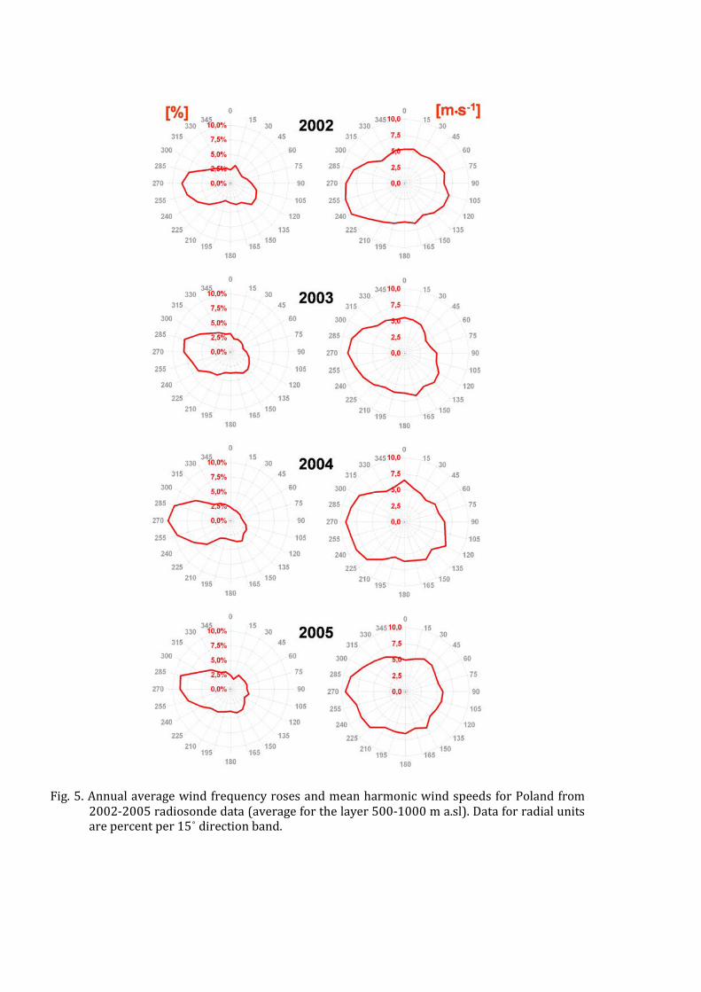
Fig. 5. Annual average wind frequency roses and mean harmonic wind speeds for Poland from

2002-2005 radiosonde data (average for the layer 500-1000 m a.sl). Data for radial units are percent per 15˚ direction band.

4.1.2. Rainfall data

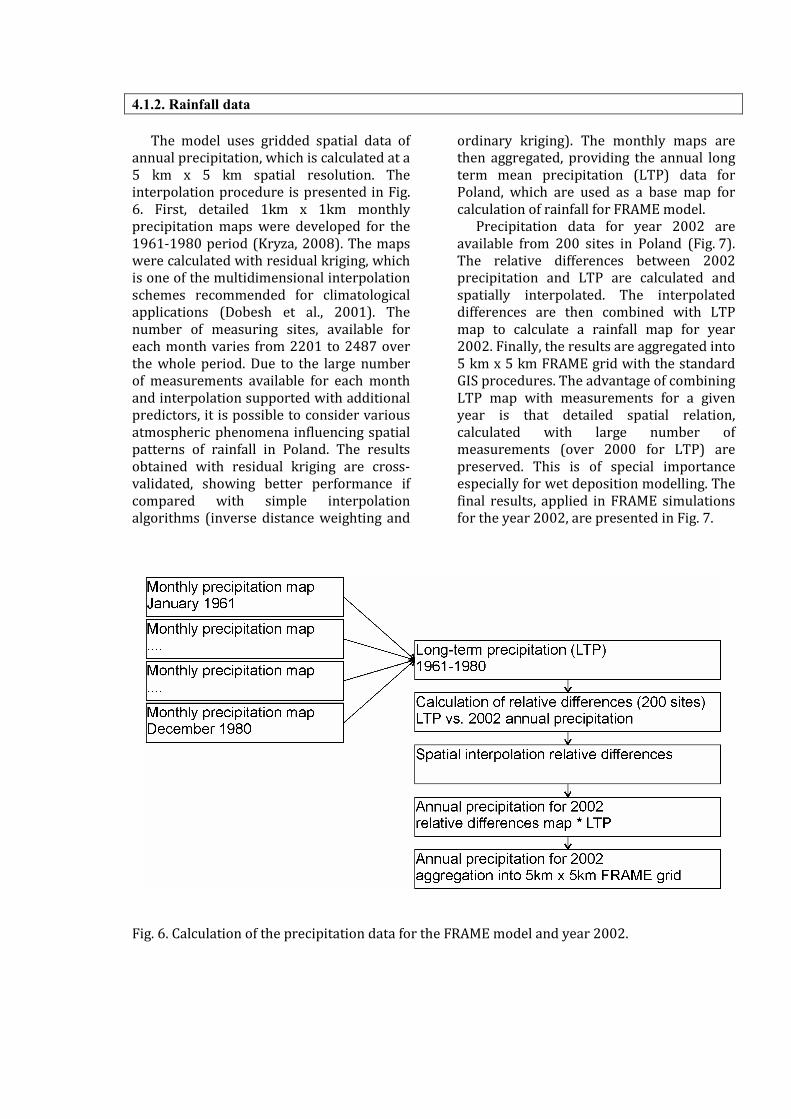
The model uses gridded spatial data of annual precipitation, which is calculated at a 5 km x 5 km spatial resolution. The interpolation procedure is presented in Fig. 6. First, detailed 1km x 1km monthly precipitation maps were developed for the 1961-1980 period (Kryza, 2008). The maps were calculated with residual kriging, which is one of the multidimensional interpolation schemes recommended for climatological applications (Dobesh et al., 2001). The number of measuring sites, available for each month varies from 2201 to 2487 over the whole period. Due to the large number of measurements available for each month and interpolation supported with additional predictors, it is possible to consider various atmospheric phenomena influencing spatial patterns of rainfall in Poland. The results obtained with residual kriging are cross-validated, showing better performance if compared with simple interpolation algorithms (inverse distance weighting and

ordinary kriging). The monthly maps are then aggregated, providing the annual long term mean precipitation (LTP) data for Poland, which are used as a base map for calculation of rainfall for FRAME model.

Precipitation data for year 2002 are available from 200 sites in Poland (Fig. 7). The relative differences between 2002 precipitation and LTP are calculated and spatially interpolated. The interpolated differences are then combined with LTP map to calculate a rainfall map for year 2002. Finally, the results are aggregated into 5 km x 5 km FRAME grid with the standard GIS procedures. The advantage of combining LTP map with measurements for a given year is that detailed spatial relation, calculated with large number of measurements (over 2000 for LTP) are preserved. This is of special importance especially for wet deposition modelling. The final results, applied in FRAME simulations for the year 2002, are presented in Fig. 7.

Fig. 6. Calculation of the precipitation data for the FRAME model and year 2002.

Fig. 7. Annual precipitation map for the years 2002-2005 (A-D) and an average for the period

1961-1980 (E).

4.1.3. The seeder-feeder effect The most effective transformation of

pollutants is caused by chemical liquid-phase reactions in clouds. Measurements show that especially in middle-size mountains commonly covered by low-level clouds, pollutant concentration are several times higher than those in precipitation (Dore et al., 1999; Błaś et al., 2002; Błaś and Sobik, 2003; Dore et al., 2007). Orographically generated low-level clouds have a substantial proportion of annual rainfall and pollutant deposition due to the “seeder-feeder” effect (SFE). It is an important atmospheric process leading to meso- or topo-scale enhancement of pre-existing precipitation and wet deposition of pollutants (Fig. 8). This phenomenon was originally presented by Bergeron (1965) to explain the enhanced rainfall observed in mountainous terrain.

Low-level feeder clouds, limited in their horizontal extend to the areas of high ground, can be washed out by rain or snow particles falling from the higher pre-existing seeder cloud (Fig. 9). The larger concentration of pollutants in feeder clouds result from the activation of aerosol into cloud droplets while the air is cooled and forced to rise. Thus the seeder-feeder process leads to a larger increase in wet deposition (Fournier et al., 2005a). The most efficient deposition is typically on the most upwind slope of the first orographic barrier, which consequently shelter the successive hill peaks downwind.

In a maritime climate at mid-latitudes, such as the United Kingdom, annual precipitation is dominated by frontal rainfall (Dore et al., 2007). In such circumstances, the humidity of the boundary layer is often close to saturation, and orographic clouds can be formed more frequently than in Poland, where a more continental climate prevails (Sobik et al., 2001). Dore et al. (1999) suggest that the increase of annual precipitation with altitude is less significant in Poland than for an equivalent altitude

change in the more maritime mid-latitude climate of the United Kingdom.

In Poland convective precipitation makes a more important contribution to total annual rainfall than in the UK, and it does not generally occur in the presence of cap clouds so that there should be no enhancement of rainfall with altitude due to scavenging by “seeder-feeder” effect in such conditions. One would therefore expect the SFE to be less influential in Poland over a long period of time. It was observed that in the UK in upland regions, as compared with the surrounding lowlands, the SFE was typically accompanied by a doubling in rainfall amount and a tripping in pollutant deposition (Dore et al., 1992; Fournier et al., 2004, 2005a). For mountainous areas in Poland the figures are 50%, and a doubling, respectively (Dore et al., 1999).

It is therefore of certain importance to consider the SFE on increasing wet pollutant deposition at the national scale. A parameterisation of the SFE is included in the FRAME model by application of the method proposed by Dore et al. (1992) and Fournier et al. (2005b). FRAME incorporates the dependence of orographic rainfall by considering two components of rainfall: non-orographic precipitation and orographic precipitation. The distinction threshold value estimated for the year 2002 is 700 mm. This is an average precipitation amount for sea-level in the UK and lowland area in Poland. Over the areas where rainfall exceeds 700 mm, it is assumed that this excess rainfall is due to orographic effects, and the scavenging coefficient is doubled. This method partly incorporates convective rainfall which occurs mainly inland during the summer when the SFE does not operate. For the UK simulation, the directional orographic precipitation model of Fournier et al. (2005a; 2001) was used to distinguish between orographic and non-orographic precipitation.

Fig. 8. Seeder-feeder mechanism.

Fig. 9. Two levels of cloud; frontal, pre-existing seeder cloud and orographic (feeder cloud) formed over Table Mts. in Republic of South Africa.

4.2. EMISSION INVENTORY 4.2.1. Introduction

Currently the FRAME model simulates transport, chemistry and deposition of three chemical families: oxidised sulphur and nitrogen and reduced nitrogen. Spatial information on the annual emission of these species has to be provided as an input data. In general, two types of sources are considered. Emissions from point sources are treated individually with the plume rise model. Gridded information on area emission are provided with the 5 km x 5 km model resolution. High resolution of the emission inventory also allows

representation of the main roads, which is important for NOx. The aim of this chapter is to describe the emission data that are used in the current version of the FRAME-PL model. Point sources emissions are taken mainly form the EPER (European Pollutant Emission Register) database and the number and location of point sources is briefly described below. For area sources, which are the main topic of the chapter, a method of spatial distribution is presented and results are compared with the EMEP emission inventory.

4.2.2. Input data and methods NATIONAL EMISSION INVENTORY

National total emission of SO2, NOx and NH3, together with other atmospheric pollutants, is annually reported by the Institute of Environmental Protection (IEP) over the 1980-2005 period. The IEP inventory reports are prepared to satisfy the needs of the UNECE Convention on Long-range Transboundary Air Pollution (CLRTAP) and its Protocols (including EMEP Programme), Eurostat and European Environmental Agency.

Total emission calculated by IEP is divided into the SNAP (Selected Nomenclature for sources of Air Pollution) sectors (Tab. 1). In this work 2002 is the year of interest, because for this year detailed census data, needed for spatial disaggregation of national emission totals, are available from the National Statistical Office (2006). Total national emission of S-SO2, N-NOx and N-NH3 in 2002 was 727.7, 238.8 and 267.5 Gg respectively (Olendrzyński et al., 2004). For SO2, over 75% of total emission comes from SNAP sectors 01, 03 and 04, which are considered here as point sources (Fig. 10). For NOx, over 47% of total emission origin from first, third and fourth SNAP sectors. Large amounts of sulphur (22%) and nitrogen (11%) oxides are emitted from commercial

and residential combustion (SNAP sector 02) and are treated here as area sources. A similar approach is used for example by King et al. (2006) and Dore et al. (2007). Almost 30% of total NOx emission come from road transport (SNAP sector 07), while this source contributes less than 3% of total SO2 emission. SNAP sector 07 is treated as a linear source, but is spatially aggregated to the 5 km x 5 km grid and provided to the FRAME model in this form.

Large amounts of NOx (over 11% of national total emission) are emitted from off-road transport (SNAP sector 08). In this case, agricultural machinery is the main source and only this source is considered here and treated as area emission, both for NOx and SO2 (0.5% of total emission). For reduced nitrogen, almost 97% of national total emission is of agricultural origin (SNAP sector 10), both from fertilizer application and animal breading. All these sources are treated as area sources. Only 1% of total NH3 emission comes from production processes, and is provided here by the EPER database as point sources. Waste treatment and disposal, contributing 2.5% of total emission, is not considered due to lack of data needed to provide the spatial (gridded) information for the FRAME model.

Tab. 1. SNAP/CORINAIR sectors considered and type of emission source.

Source type SNAP SNAP/CORINAIR Activity

SO2 NOx NH3

01 Combustion in energy and transformation industries

Point sources Point sources Not considered

02 Non-industrial combustion plants Area sources Area sources Not considered

03 Combustion in manufacturing

industry Point sources Point sources Not considered

04 Production processes Point sources Point sources Point sources

05 Extraction and distribution of fossil

fuels and geothermal energy Not considered Not considered Not considered

06 Solvent and other product use Not considered Not considered Not considered 07 Road transport Line/area sources Line/area sources Not considered 08 Other mobile sources and machinery Area sources Area sources Not considered 09 Waste treatment and disposal Not considered Not considered Not considered 10 Agriculture Not considered Not considered Area sources 11 Other sources and sinks Not considered Not considered Not considered

EMISSION FROM POINT SOURCES - EPER DATABASE

In an atmospheric transport model such as FRAME, correct representation of the height at which pollutant gases are emitted to the atmosphere is an important consideration (Tadmor, 1967; Dore et al., 2006b).

With emission heights underestimated, modelled concentration close to the ground will be too high, resulting in overestimate of gaseous dry deposition in the vicinity of the source. With emission heights set too high, the model will overestimate the fraction of emission which escapes the local area and

contributes to long range transport of pollutants. It also follows from this argument that the model requires a fine vertical grid spacing in order to resolve differences in emission heights. In FRAME, major point source emission of SO2 and NOx were separated from low level emission and, where available, information on stack height data was employed to input the emission at the appropriate vertical layer in the model, with the plume rise option included.

Fig. 10. National total [Gg of S or N] and SNAP sectors emissions in 2002.

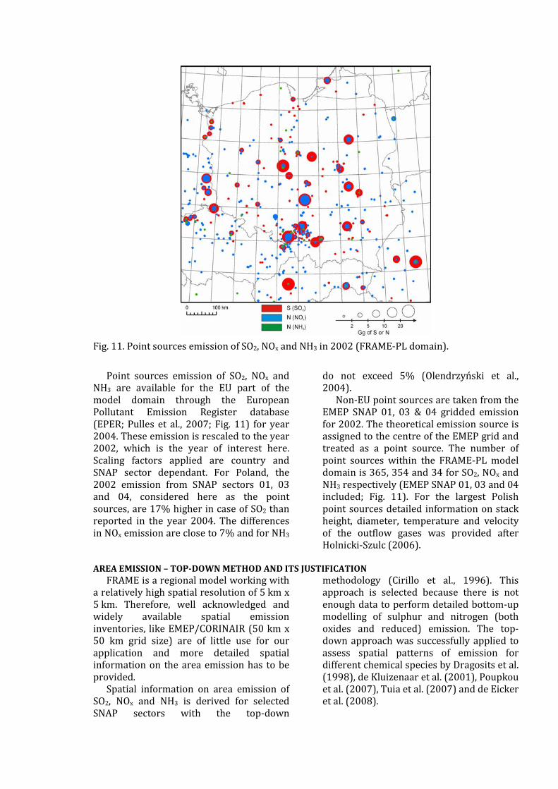
Fig. 11. Point sources emission of SO2, NOx and NH3 in 2002 (FRAME-PL domain).

Point sources emission of SO2, NOx and

NH3 are available for the EU part of the model domain through the European Pollutant Emission Register database (EPER; Pulles et al., 2007; Fig. 11) for year 2004. These emission is rescaled to the year 2002, which is the year of interest here. Scaling factors applied are country and SNAP sector dependant. For Poland, the 2002 emission from SNAP sectors 01, 03 and 04, considered here as the point sources, are 17% higher in case of SO2 than reported in the year 2004. The differences in NOx emission are close to 7% and for NH3

do not exceed 5% (Olendrzyński et al., 2004).

Non-EU point sources are taken from the EMEP SNAP 01, 03 & 04 gridded emission for 2002. The theoretical emission source is assigned to the centre of the EMEP grid and treated as a point source. The number of point sources within the FRAME-PL model domain is 365, 354 and 34 for SO2, NOx and NH3 respectively (EMEP SNAP 01, 03 and 04 included; Fig. 11). For the largest Polish point sources detailed information on stack height, diameter, temperature and velocity of the outflow gases was provided after Holnicki-Szulc (2006).

AREA EMISSION – TOP-DOWN METHOD AND ITS JUSTIFICATION

FRAME is a regional model working with a relatively high spatial resolution of 5 km x 5 km. Therefore, well acknowledged and widely available spatial emission inventories, like EMEP/CORINAIR (50 km x 50 km grid size) are of little use for our application and more detailed spatial information on the area emission has to be provided.

Spatial information on area emission of SO2, NOx and NH3 is derived for selected SNAP sectors with the top-down

methodology (Cirillo et al., 1996). This approach is selected because there is not enough data to perform detailed bottom-up modelling of sulphur and nitrogen (both oxides and reduced) emission. The top-down approach was successfully applied to assess spatial patterns of emission for different chemical species by Dragosits et al. (1998), de Kluizenaar et al. (2001), Poupkou et al. (2007), Tuia et al. (2007) and de Eicker et al. (2008).

The general idea of the top-down approach is presented by Tuia et al. (2007) and Cirillo et al. (1996, Fig. 12). The starting point is the national total emission estimates, provided by the IEP reports. Proxy variables (census and traffic data) are used to disaggregate the SNAP sectors totals into the smaller territorial division units (commune or province level). Within the commune/province emissions are assigned to the appropriate landuse classes according to the CORINE Land Cover database (Perigão and Annoni, 1997; Buetner et al., 2002).

The top-down approach was performed with the OpenSource GIS GRASS and R environment (GRASS Development Team, 2006; R Development Team, 2009). The initial resolution of the raster layers was set to 100 m x 100 m, and is equal to the resolution used for CORINE Land Cover map

(Bossard et al., 2000). Such a high resolution was necessary to avoid the initial input landuse data generalisation. The final layers were aggregated to the FRAME 5 km x 5 km grid with the standard GIS procedures. For SO2 and NOx SNAP sector 02 emission, data on heating system type are used in spatial disaggregation of sector total emission (Tab. 2). This information is available for each commune from the 2002 census. National total emission from SNAP sector 02 is firstly divided into communes. The total emission from each commune is assumed to be proportional to the total area of usable floor of inhabited dwellings using individual central heating system. Within the commune, total emission is assigned to the location of the cities and villages and is assumed to be proportional to the population of the city/village.

Tab. 2. Proxy data used for spatial disaggregation of area emission.

SNAP Proxy data

02 Usable floor of inhabited dwellings using individual central heating system at

commune level and population data. 07 Average traffic intensity (no of cars per day) 08 Number of agricultural machinery in a commune 10 Animal numbers at commune level and fertilizer consumption at province level

Fig. 12. Distribution of emission in the bottom-up (left) and top-down (right) case (after Tuia et al., 2007).

For traffic emission, data on average traffic intensity, assigned to the road network, are used as proxy information in SO2 and NOx emission downscaling. It should be mentioned that the proxy data are available only for the main roads. No information on fleet composition is used. This is the main drawback in this approach and should be solved in the future, as the traffic emission is recently gaining in importance in Poland according to the IEP reports. Driving patterns are also not included and this leads to certain simplification of the traffic emission pattern (Smith et al., 2008). In case of SO2 and NOx emission from SNAP sector 08, information on agricultural machinery in communes is used as proxy data in the national total emission disaggregation. Within each commune, total emission is assigned to the agricultural areas from the CORINE Land Cover database. No additional weights are assigned to the different agricultural land use classes.

For agricultural NH3 emission, two main sources are considered and separately disaggregated: animal breeding and fertilizer application. Emission from livestock is further divided into main animal

types: cattle, pigs, horses, sheep and hens. Information on animal number is available on commune level from the 2002 Agricultural Census and is used here to disaggregate the national total emission into the communes. Further, the total livestock-origin emission in the commune is assigned into the appropriate landuse category, depending on animals type. Cattle, horses and sheep emission are assigned to the pastures and grassland areas, pigs to pastures, grassland areas and villages, while hens are assigned to villages only. If no appropriate landuse category is reported in the commune (due the CORINE Land Cover database generalisation), average emission per hectare is calculated, passing over the landuse type. Seasonal changes in animal location (outdoor or indoor breeding) are not currently considered but should be implemented in the disaggregation procedure, as proposed by Dragosits et al. (1998). Data on fertilizer consumption are available only on the province level. National total emission is divided into the provinces. Within each province, emission is assigned to the arable land, according to the CORINE Land Cover map.

4.2.3. Area emission – results and validation GENERAL DESCRIPTION

The highest emission of sulphur and nitrogen oxides, calculated with top-down approach, is from the large cities (Fig. 13). These are the areas where large emission from residential and commercial combustion is combined with high traffic intensity, which is of special importance for nitrogen oxides emission. High NOx emission is also noticeable along the main roads, which is not the case of the coarse resolution EMEP/CORINAIR inventory. This example shows how important the spatial resolution is in case of emission and, further, in transport, concentration and depositions modelling. Detailed spatial information on emission, concentration and deposition is needed for example in critical level and loads assessment.

In case of SO2, high emission over the Upper Silesia region is noticeable. These are related to large hard coal consumption in

residential and commercial combustion. Coal is mined there, widely available, and is a relatively cheap source of energy compared with other fuels.

Central Poland is the traditional region of intensive agricultural activity and, therefore, the area with the largest agricultural emission of reduced nitrogen (Fig. 14 a-c). In the region high population of breeding animals (mainly pigs and hens) is combined with the large fertilizer consumption due to intensive farming. Data on fertilizer consumption are available only on the province level. This affects the spatial pattern of NHx emission from this activity and the provinces can be distinguished on the final emission map (Fig. 14d). This should be considered as a drawback, but no detail census data on fertilizer application are currently available.

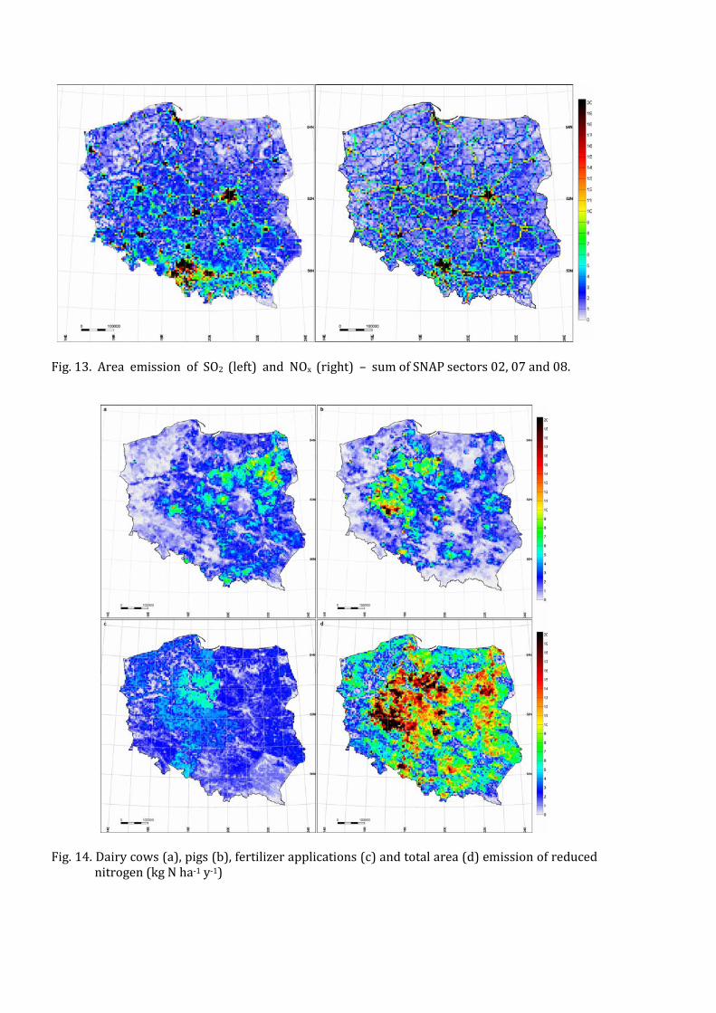
Fig. 13. Area emission of SO2 (left) and NOx (right) – sum of SNAP sectors 02, 07 and 08.

Fig. 14. Dairy cows (a), pigs (b), fertilizer applications (c) and total area (d) emission of reduced

nitrogen (kg N ha-1 y-1)

Fig. 15. FRAME-PL and EMEP emission, (a) SO2, (b) NOx, (c) NH3.

EVALUATION OF THE AREA EMISSION ESTIMATES

Validation of the area emission estimates is made here by comparison with an independent emission inventory (EMEP WebDAB; Vestreng et al., 2002, 2004) and, secondly, by comparing the FRAME modelled air concentration of atmospheric gaseous pollutants with available measurements. These validation procedures are suggested by Cirillo et al. (1996) and Reis (2005). In this chapter, only the comparison with the EMEP emission inventory is presented. Modelled air concentration is compared with measurements as a part of the FRAME-PL model validation (section 6).

The results of spatial disaggregation of national total emission are compared with the EMEP/WebDAB emission inventory as this is the only available and consistent source covering whole Poland. It should be stressed that the EMEP emission inventory

is prepared with 50 km x 50 km spatial resolution and each EMEP grid cell covers 100 FRAME grid cells. To compare the FRAME-PL and EMEP emission inventories, the former is aggregated into the EMEP grid resolution. In general, there is a good correlation between EMEP and FRAME-PL (aggregated to the EMEP grid) for sulphur and nitrogen oxides (Fig. 15). In the case of SO2 emission, there are some grids for which FRAME-PL emission are close to zero, while EMEP emission being considerably higher (Fig. 15). These differences should be attributed to the shipping emission, which are not currently included in the FRAME-PL inventory. The scattering is larger for reduced nitrogen emission. This might be the result of the detailed proxy and land cover data used for the spatial disaggregation of the NHx emission in our data set (Erisman et al., 1993).

4.3. SUMMARY

The emission inventory, needed for SO2, NOx and NH3 transport, concentration and deposition modelling with FRAME-PL, was described for both point and area sources. The point source emissions are taken from the European Pollution Emission Register database for the year 2004. Country and SNAP sector dependant scaling factors are used to rescale the 2004 emission to the year 2002, which is the year of interest here. This is the main drawback in the case of the point sources, bearing in mind that the point sources emission data are collected in Poland, but not widely available.

For area emission, the top-down approach is used here to downscale the national total emission estimates, as there is not enough input data to fulfil the needs of the bottom-up scheme. The top-down approach has some certain limitations, as it is based on the proxy spatial data. The correct selection of the auxiliary information is therefore important, but limited by the data availability. The spatial patterns of the FRAME emission inventory

are however in general agreement with the EMEP/CORINAIR estimates. The largest differences are for reduced nitrogen. This can be attributed to the detailed data used for the agricultural emission disaggregation, including individual treatment of fertilizer and different animals emission. Good agreement between the FRAME modelled air concentration of sulphur and nitrogen oxides with the measurements, presented in the further chapter (6.2.2), also suggests that the simple top-down approach is quite reliable and effective.

Despite the limited input data, some improvements in the spatial disaggregation of national total emission are possible and should be applied in the future. These particularly concern the traffic emission, where emission from different vehicles should be treated separately. Reduced nitrogen emission from animal breeding could also be improved by taking into account the seasonal changes in animal location (outdoor or indoor breeding).

4.4. REFERENCES Bergeron, T., 1965, One the low-level

redistribution of atmospheric water caused by orography. Proceedings of the International Conference on Cloud Physics, Tokyo, 1965, pp. 96-100.

Błaś, M., Sobik, M., Quiel, F., Netzel, P., 2002, Temporal and spatial variations of fog in the Western Sudety Mts., Poland. Atmospheric Research 64, 19-28.

Błaś, M., Sobik, M., 2003, Natural and human impact on pollutant deposition in mountain ecosystems with the Sudetes as an example. Studia Geograficzne 75, 420-438.

Bossard, M., Feranec, J., Otahel, J., 2000, CORINE Land Cover Technical Guide-Addendum 2000, European Environmental Agency, Copenhagen.

Brimblecombe, P., 1996, Air composition and Chemistry (2nd Edition ed.), Cambridge University Press, Cambridge 1996.

Buettner, G., Feranec, J., Jaffrain, G., 2002, Corine land cover update 2002. Technical guidelines. EEA, pp. 56.

Cirillo, M.C., De Lauretis, R., Del Ciello, R., 1996, Review study on European urban emission inventories, European Topic Centre on Air Emission, pp. 35.

De Eicker, M.O., Zah, R., Triviño, R., Hurni, H., 2008, Spatial accuracy of a simplified dissagregation method for traffic emissions applied in seven mid-sized Chilean cities, Atmospheric Environment 42, 1491-1502.

De Kluizenaar, Y., Aherne, J., Farrell, E.P., 2001, Modelling the spatial distribution of SO2 and NOx emissions in Ireland, Environmental Pollution 112, 171-182.

Dobesch, H., Tveito, O.E., Bessemoulin, P., 2001, Geographic Information Systems in Climatological Application, DNMI-Report 13/01 KLIMA, pp. 49

Dore, A.J., Choularton, T.W., Fowler, D., 1992, An improved wet deposition map of the United Kingdom incorporating the topographic dependence of rainfall concentrations. Atmospheric Environment 26A, 1375-1381.

Dore, A.J., Sobik, M., Migała, K., 1999, Patterns of precipitation and pollutant deposition in the Western Sudety Mountains, Poland. Atmospheric Environment 33, 3301-3312.

Dore, A.J., Vieno, M., Fournier, N., Weston, K.J., Sutton, M.A., 2006a, Development of a new wind rose for the British Isles using radiosonde data and application to an atmospheric transport model. Quarterly

Journal of the Royal Meteorological Society 132, 2769-2784.

Dore, A.J., Vieno, M., MacDougal, M., Kryza, M., Błaś, M., Hall, J., Dosio, A., Tang, S., Smith, R., Sutton, M., 2006b, Modelling the deposition and concentration of long range air pollutants: Final Report , DEFRA, pp 84.

Dore, C.J., Watterson, J.D., Murrells, T.P., Passant, N.R., Hobson, M.M., Choudrie, S.L., Thistlethwaite, G., Wagner, A., Jackson, J., Li, Y., Bush, T., King, K.R., Norris, J., Coleman, P.J., Walker, C., Stewart, R.A., Goodwin, J.W.L., Tsagatakis, I., Conolly, C., Downes, M.K., Brophy, N., Hann, M.R., 2007, UK emissions of air pollutants 1970 to 2005, NAEI, pp. 197.

Dragosits, U., Sutton, M.A., Place, C.J., Bayley, A.A., 1998, Modelling the spatial distribution of agricultural ammonia emissions in the UK, Environmentla Pollution 102(S1), 195-203.

Erisman, J.W., Verslius, A.H., Verplanke, T.A.J.W., de Haan, D., Anink, D., van Elzakker, B.G., Mennen, M., van Aalst, R.M., 1993, Monitoring the dry deposition of SO2 in the Netherland: results for grassland and heather vegetation, Atmospheric Environment 27A, 1153-1161.

Fournier, N., Weston, M.A., Sutton, M.A., Dore, A.J., 2001, Inclusion of an improved parametrisation of the wet deposition process in an atmospheric transport model. Proceedings of the 25th NATO/CCMS International technical meeting on air pollution modeling and its application. Louvain-la-Neuve, Belgium, 15-19 October, 265-273.

Fournier, N., Dore, A.J., Vieno, M., Weston, K.J.W., Dragosits. U., Sutton, M.A., 2004, Modelling the deposition of atmospheric oxidised nitrogen and sulphur to the United Kingdom using a multi-layer long-range transport model. Atmospheric Environment 38(5), 683-694.

Fournier, N., Weston, K.J.W., Dore, A.J., Sutton, M.A., 2005a, Modelling the wet deposition of reduced nitrogen over the British Isles using a multi-layer atmospheric transport model. Quarterly Journal of the Royal Meteorological Society 131, 703-722.

Fournier, N., Tang, Y.S., Dragisits, U., Kluizenaar, Y., Sutton, M.A., 2005b, Regional atmospheric budgets of reduced nitrogen over the British Isles assessed using a multi-layer atmospheric transport model. Water, Air & Soil Pollution 162, 331-351.

GRASS Development Team, 2006. Geographic Resources Analysis Support System (GRASS)

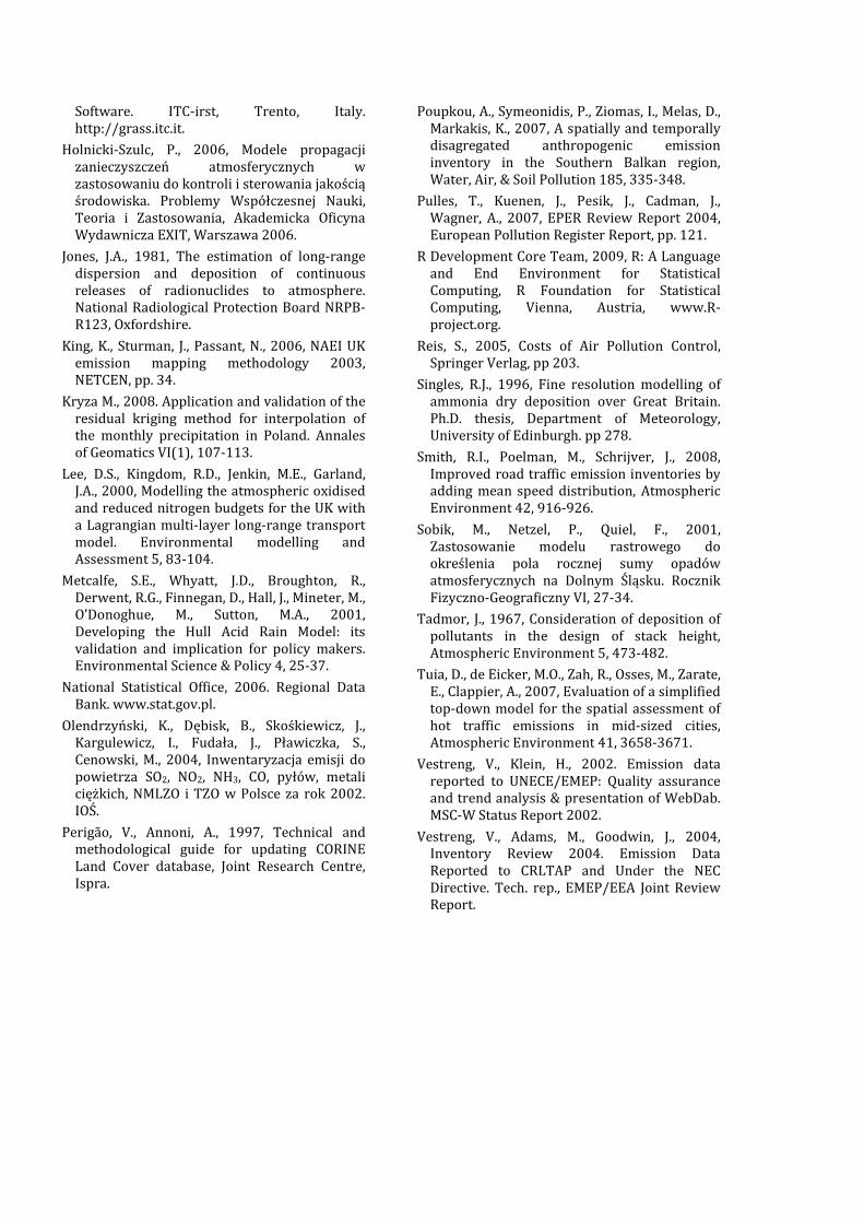
Software. ITC-irst, Trento, Italy. http://grass.itc.it.

Holnicki-Szulc, P., 2006, Modele propagacji zanieczyszczeń atmosferycznych w zastosowaniu do kontroli i sterowania jakością środowiska. Problemy Współczesnej Nauki, Teoria i Zastosowania, Akademicka Oficyna Wydawnicza EXIT, Warszawa 2006.

Jones, J.A., 1981, The estimation of long-range dispersion and deposition of continuous releases of radionuclides to atmosphere. National Radiological Protection Board NRPB-R123, Oxfordshire.

King, K., Sturman, J., Passant, N., 2006, NAEI UK emission mapping methodology 2003, NETCEN, pp. 34.

Kryza M., 2008. Application and validation of the residual kriging method for interpolation of the monthly precipitation in Poland. Annales of Geomatics VI(1), 107-113.

Lee, D.S., Kingdom, R.D., Jenkin, M.E., Garland, J.A., 2000, Modelling the atmospheric oxidised and reduced nitrogen budgets for the UK with a Lagrangian multi-layer long-range transport model. Environmental modelling and Assessment 5, 83-104.

Metcalfe, S.E., Whyatt, J.D., Broughton, R., Derwent, R.G., Finnegan, D., Hall, J., Mineter, M., O’Donoghue, M., Sutton, M.A., 2001, Developing the Hull Acid Rain Model: its validation and implication for policy makers. Environmental Science & Policy 4, 25-37.

National Statistical Office, 2006. Regional Data Bank. www.stat.gov.pl.

Olendrzyński, K., Dębisk, B., Skośkiewicz, J., Kargulewicz, I., Fudała, J., Pławiczka, S., Cenowski, M., 2004, Inwentaryzacja emisji do powietrza SO2, NO2, NH3, CO, pyłów, metali ciężkich, NMLZO i TZO w Polsce za rok 2002. IOŚ.

Perigão, V., Annoni, A., 1997, Technical and methodological guide for updating CORINE Land Cover database, Joint Research Centre, Ispra.

Poupkou, A., Symeonidis, P., Ziomas, I., Melas, D., Markakis, K., 2007, A spatially and temporally disagregated anthropogenic emission inventory in the Southern Balkan region, Water, Air, & Soil Pollution 185, 335-348.

Pulles, T., Kuenen, J., Pesik, J., Cadman, J., Wagner, A., 2007, EPER Review Report 2004, European Pollution Register Report, pp. 121.

R Development Core Team, 2009, R: A Language and End Environment for Statistical Computing, R Foundation for Statistical Computing, Vienna, Austria, www.R-project.org.

Reis, S., 2005, Costs of Air Pollution Control, Springer Verlag, pp 203.

Singles, R.J., 1996, Fine resolution modelling of ammonia dry deposition over Great Britain. Ph.D. thesis, Department of Meteorology, University of Edinburgh. pp 278.

Smith, R.I., Poelman, M., Schrijver, J., 2008, Improved road traffic emission inventories by adding mean speed distribution, Atmospheric Environment 42, 916-926.

Sobik, M., Netzel, P., Quiel, F., 2001, Zastosowanie modelu rastrowego do określenia pola rocznej sumy opadów atmosferycznych na Dolnym Śląsku. Rocznik Fizyczno-Geograficzny VI, 27-34.

Tadmor, J., 1967, Consideration of deposition of pollutants in the design of stack height, Atmospheric Environment 5, 473-482.

Tuia, D., de Eicker, M.O., Zah, R., Osses, M., Zarate, E., Clappier, A., 2007, Evaluation of a simplified top-down model for the spatial assessment of hot traffic emissions in mid-sized cities, Atmospheric Environment 41, 3658-3671.

Vestreng, V., Klein, H., 2002. Emission data reported to UNECE/EMEP: Quality assurance and trend analysis & presentation of WebDab. MSC-W Status Report 2002.

Vestreng, V., Adams, M., Goodwin, J., 2004, Inventory Review 2004. Emission Data Reported to CRLTAP and Under the NEC Directive. Tech. rep., EMEP/EEA Joint Review Report.

5. FRAME MODEL RESULTS – CONCENTRATION AND DEPOSITION OF AIR POLLUTANTS IN POLAND

In this chapter, FRAME-PL modelled

spatial patterns of air concentration and depositions are presented and briefly discussed. EMEP model results are also presented for visual comparison.

The highest concentration of SO2, NOx and NH3 in Poland for the year 2002 is estimated by the FRAME model close to the low level (area) emission sources (Fig. 16, 17, 18). For SO2, the highest annual mean concentrations are typically calculated for the urban areas, and are attributed to large emissions from SNAP sector 2 (residential combustion) supported by emission from industry. For nitrogen oxides, high concentrations are related to main roads and large urban areas, with the emission from transport and residential combustion being mainly responsible. Elevated NOx concentrations are evident along the main roads for FRAME, but not for the coarse resolution EMEP model. The highest NH3 air concentrations are calculated for the areas of intensive agriculture production in central Poland, i.e. in the vicinity of high emission from fertilizer application and animal breeding. Also the EMEP model predicts high concentrations for that area although the FRAME calculated spatial pattern is more complex due to the higher spatial resolution of the FRAME model grid. The recent findings, presented by Dore et al. (2007) and Hallsworth et al. (2009), show that in some cases 5 km x 5 km resolution of the FRAME model is still insufficient to properly reflect large local gradients of reduced nitrogen emission/air concentration and there might be strong sub-grid variations in ammonia concentration in the vicinity of emission sources. These findings are supported by the earlier papers of Skjøth et al. (2004) and Hertel et al. (2006), suggesting 400 m x 400 m grid size for modelling of reduced nitrogen air concentration.

The grid-average dry depositions of sulphur and nitrogen (both oxidised and reduced, Fig. 19, 20, 21), modelled with FRAME, have quite similar spatial patterns to air concentrations of SO2 and NOx

discussed above. The highest dry depositions are calculated for the areas of large emission. Dry deposition of oxides sulphur is associated with areas of high SO2 emission, as well as oxidised nitrogen deposition is the highest over the urbanized areas where emission from vehicle exhausts are large. Due to the low-level emission of NH3 and its reactive nature, much ammonia is deposited into the grid square of emission, so that the deposition pattern is closely correlated to the spatial distribution of emission. Remote mountainous areas in the south have dry deposition of reduced nitrogen well below 1 kg N ha-1 y-1. However, dry deposition of oxidised sulphur and nitrogen for these areas is quite large which may be attributed to the large amounts of the pollutants emitted from point sources. The other explanation for the large dry depositions over the remote mountainous areas to the south is the transboundary transport, with the prevailing winds from W and SW (i.e. from the industrialized areas of Czech Republic and Germany). The latest is supported by the EMEP reports (Klein et al., 2004), and will be further investigated also with the FRAME model.

As aerosol particles are associated with long range transport, the areas of high wet deposition are not related to areas of high emission of primary pollutants but more closely correlated to areas of high rainfall. Therefore, the mountainous areas in the south suffer from large wet deposition of oxidised sulphur and nitrogen and reduced nitrogen (Fig. 22, 23, 24). Especially, in case of NO3-, wet deposition over the source areas is few times lower than over the remote mountainous regions. This is also attributed to the seeder-feeder effect, which is represented in the FRAME model by an enhanced scavenging coefficient for orographic precipitation. In particular the mountain areas of the Western Sudety Mts. and Beskid Żywiecki, deposition exceeds 15 kg N ha-1 y-1 for NH4+ and NO3- and 18 kg S ha-1 y-1 for SO4--. The spatial pattern of wet deposition calculated with the EMEP model

is quite different. The EMEP model gives lower depositions over the mountainous areas, if compared with FRAME estimates. The main reason for this difference is that orographic enhancement of ion concentration in precipitation is not considered in the EMEP model. Furthermore, there are difficulties

associated with proper meteorological modelling of orographic precipitation using a model grid resolution of 50 km. As demonstrated by Dore et al. (1999, 2007), wet deposition in upland regions can vary significantly at a 1 km distance which is unresolved by the model 5 km grid squares.

Fig. 16. FRAME and EMEP modelled SO2 air concentration.

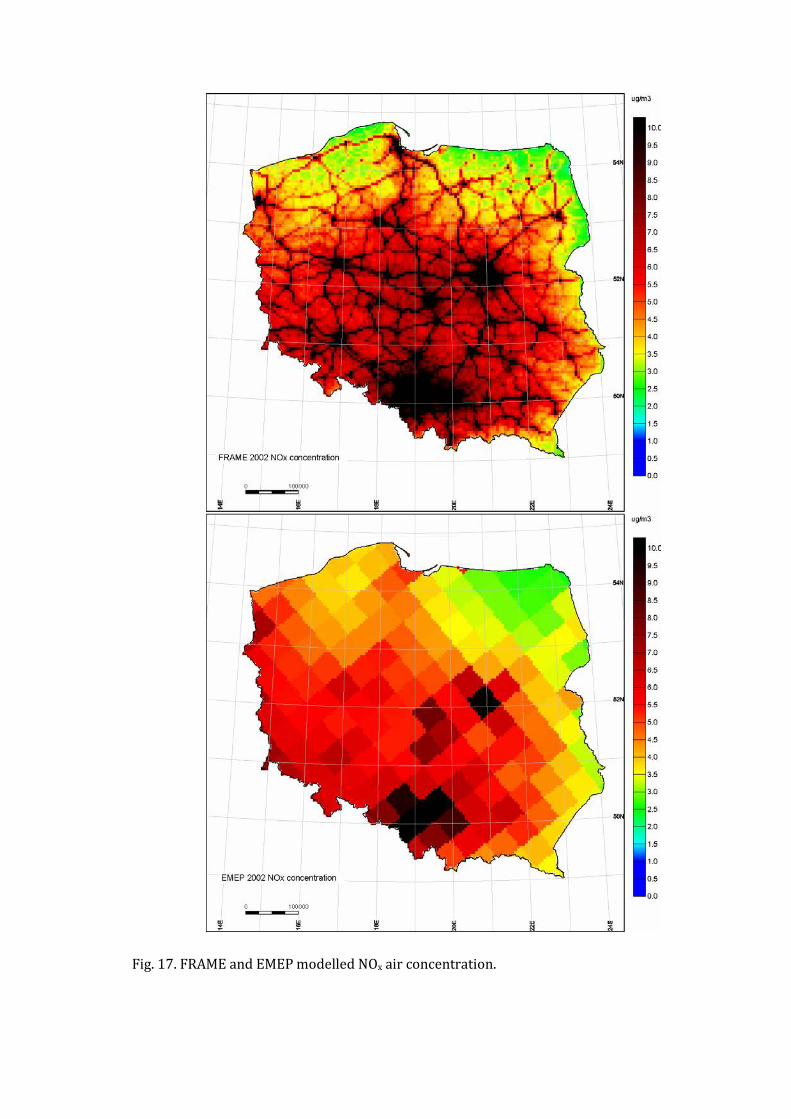
Fig. 17. FRAME and EMEP modelled NOx air concentration.

Fig. 18. FRAME and EMEP modelled NH3 air concentration.

Fig. 19. FRAME and EMEP modelled dry depositions of oxidised sulphur.

Fig. 20. FRAME and EMEP modelled dry depositions of oxidised nitrogen.

Fig. 21. FRAME and EMEP modelled dry depositions of reduced nitrogen.

Fig. 22. FRAME and EMEP modelled wet depositions of oxidised sulphur.

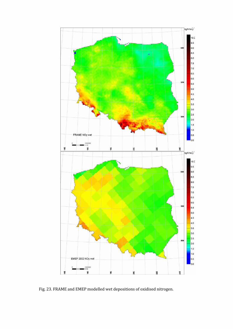
Fig. 23. FRAME and EMEP modelled wet depositions of oxidised nitrogen.

Fig. 24. FRAME and EMEP modelled wet depositions of reduced nitrogen.

REFERENCES Dore, A.J., Sobik, M., Migała, K., 1999, Patterns of

precipitation and pollutant deposition in the Western Sudety Mountains, Poland. Atmospheric Environment 33, 3301-3312.

Dore, A.J., Theobald, M.R., Kryza, M., Vieno, M., Tang, S.Y., Sutton, M.A., 2007, Modelling the deposition of Reduced Nitrogen at different scales in the United Kingdom. Proc. 29th NATO/SPS International Technical Meeting on Air Pollution Modelling and its Application, Aveiro, Portugal, 24-28 September 2007 (in press).

Hallsworth, S., Dore, A.J., Bealey, W.J., Dragosits, U., Vieno, M., Hellsten, S., Tang, Y.S., Sutton, M.A., 2009, The role of indicator choice in quantifying the threat of atmospheric ammonia to the ‘Natura 2000’ network.

Environmental Science and Policy (under review).

Hertel, O., Skjøth, C.A., Løfstrøm, P., Geels, C., Frohn, L.M., Ellermann, T., Madsen, P.V., 2006, Modelling nitrogen deposition on a local scale – a review of the current state of the art. Environmental Chemistry 3, 317-337.

Skjøth, C.A., Hertel, O., Gyldenkærne, S., Ellermann, T., 2004, Implementing a dynamical ammonia emission parameterization in the large-scale air pollution model ACDEP. Journal of Geophysical Research 109, 1-13.

Klein, H., Wind, P., van Loon, M., 2004, Transboundary air pollution by main pollutants (S, N, O3) and PM: Poland. MSC-W Data Nite 1/2004.

6. EVALUATION OF THE FRAME MODEL RESULTS

Evaluation is the procedure that allows assessment of the degree to which a model is an accurate representation of the real world (Sornette et al., 2007). Atmospheric transport models are widely used for numerous environmental studies, as well as national and international bodies e.g. to evaluate emission reduction scenarios and to look for the most cost/environmental effect efficiency of the abatement policy. Therefore these end-users need to have knowledge on the uncertainty related with the atmospheric transport models estimates, as this may by influential on their conclusions and decisions (Metcalfe et al., 2005). A detailed description of the model validation procedures was described e.g. by Sofiev (1999), Seinfeld and Pandis (2006).

Here, the FRAME-PL model results are compared with: � Measured annual average air

concentration and annual wet deposition (data-model inter-comparison). This is a direct assessment of the model accuracy.

� The EMEP model results for air concentration, wet and dry deposition.

� EMEP and CIEP calculated wet, dry and total deposition budget for Poland.

The FRAME model has also been extensively verified for the UK including comparison with measurements from monitoring network and the results were presented by Dore et al. (2007b). The results of the FRAME-UK model were also compared with the EMEP and CBED model estimates for the UK.

6.1. DATA AND METHODS

6.1.1. Measurement data

The most straightforward (and demanding) way to validate the model results is to compare them with the available measurements (Metcalfe et al., 2001, 2005; Seinfeld and Pandis 2006). Information on measured mean annual air concentration of SO2 are taken after Skotak et al. (2003) while NO2 measurements for the year 2002 are from the European Air quality data base (AirBase; Mol and Leeuw, 2005). The air quality database consists of long standing time series of air quality measurement data and their statistics for a representative selection of stations and for a number of pollutants. To ensure the quality of the measurement data, only the sites with at least 90% completeness of daily measurements are considered. For the model validation, 75 sites for SO2 and 21 for NO2 are available. NH3 air concentration measurements are not performed routinely on the monitoring network in Poland. Over the year 2002, only three EMEP sites with ammonia measurements were operating and are used here as a complementary measure of the model performance.

In the case of wet deposition, EMEP, as well as the World Meteorological

Organisation (WMO), recommend use of wet-only collectors because of smaller influence of dry deposition and contamination on the measurement (Allan, 2004; EMEP/CCC-Report 1/95). In theory, wet deposition is best measured using wet-only samplers, which, in contrast to bulk samplers, are covered by a lid during dry periods and open whenever precipitation is detected by a sensor. Differences in the chemical composition of precipitation collected by wet-only and bulk collectors have been assessed in a number of comparative studies (Stedman et al., 1990; 1992; Aikawa et al., 2003; Staelens et al., 2005). Wet depositions of oxidised sulphur and nitrogen as well as reduced nitrogen in Poland are measured with wet-only samplers at 25 synoptic weather stations operated by the Institute of Meteorology and Water Management (Tab. 3). All these sites are used here to evaluate wet depositions calculated with the FRAME-PL model. Dry deposition measurements of sulphur and nitrogen are not available for the model domain. The results are therefore validated only by comparison with the EMEP-Unified model results.

Tab. 3. Monitoring stations with wet-only measurements of precipitation chemistry in Poland.

Geographical position Nr Station

Code number Φ λ

Altitude (m a.s.l.)

1 Świnoujście 200 53°55' 14°14' 6 2 Łeba 120 54°45' 17°32' 2 3 Gdańsk 140 54°24' 18°42' 2 4 Suwałki 195 54°08' 22°57' 184 5 Chojnice 235 53°43' 17°32' 165 6 Olsztyn 272 53°46' 20°25' 133 7 Gorzów Wlkp. 300 52°45' 15°17' 72 8 Toruń 250 53°03' 18°35' 69 9 Białystok 295 53°06' 23°10' 148

10 Zielona Góra 400 51°56' 15°32' 192 11 Poznań 330 52°25' 16°51' 83 12 Warszawa-Okęcie 375 52°10' 20°58' 108 13 Kalisz 435 51°47' 18°05' 138 14 Sulejów 469 51°21' 19°52' 188 15 Włodawa 497 51°33' 23°32' 177 16 Legnica 415 51°12' 16°12' 122 17 Wrocław-Strachowice 424 51°06' 16°56' 120 18 Śnieżka 510 50°44' 15°44' 1603 19 Kłodzko 520 50°26' 16°39' 355 20 Racibórz 540 50°03' 18°12' 205 21 Katowice 560 50°14' 19°02' 284 22 Kraków Balice 566 50°05' 19°48' 237 23 Sandomierz 585 50°42' 21°43' 217 24 Kasprowy Wierch 650 49°14' 19°59' 1991 25 Lesko 690 49°28' 22°21' 420

6.1.2. Comparison with the EMEP-Unified model

Comparison with other models is an

important step of the validation procedure, which was performed for example by Dore at al. (2007b; FRAME, EMEP and CBED model intercomparison), and Metcalfe et al. (2001, 2005) to evaluate the HULL model performance. Spatial patterns of the FRAME-PL modelled air concentration and depositions (wet and dry) were compared with the results calculated by well established EMEP-Unified model (Simpson et al., 2003; Fagerli et al., 2004). Of special importance are the differences in model formulation. FRAME is a Lagrangian, statistical trajectory model based on average meteorology. In contrary, EMEP is a complex Eulerian model driven by the modelled meteorology provided by the HIRLAM model (Bjørge and Skålin, 1995; Sandnes and Tsyro, 2000). The models differ also in horizontal and vertical resolution. Further differences are discussed below. According to the author’s best knowledge, EMEP is the main and most up to date source of the spatial information on annual average air concentration and

depositions of chemical species of interest (sulphur and nitrogen compounds) at a national scale for Poland.

It should be stressed that both models are based on different assumptions and also that the differences in the input information are large. The most important may be listed as follow: � Lagrangian (FRAME) vs. Eulerian (EMEP)

approach. � FRAME straight line trajectories and

average meteorology vs. detailed representation of the meteorology in the EMEP model.

� High spatial resolution of the FRAME model (5km x 5km grid) vs. coarse 50km x 50km EMEP grid.

� High vertical resolution (33 layers, 1 m depth at the ground) of the FRAME model and 50 m thick 1st layer of the EMEP model.

The substantial differences of the two models make this part of the validation especially important. This gives the answer to the question if the simple statistical FRAME model is able to calculate the

regional patterns of the annual average air concentration and depositions.

The FRAME-EMEP intercomparison is two-fold. First, the FRAME air concentration and deposition (dry and wet) data are aggregated into the 50 km x 50 km EMEP grid. This unifies the spatial resolution of the two models and assures “fair” FRAME-EMEP inter-comparison. A linear regression analysis is performed describing correlation between the corresponding EMEP and (aggregated) FRAME grid cells. In case of air concentration, the comparison is performed for sulphur and nitrogen oxides and

ammonia. For wet and dry deposition, SOx, NOy and NHx are considered. This part of the validation procedure allows us to quantitatively assess the general agreement of the results of the two models, despite the different spatial resolution. In the second step, EMEP data are regridded into the 5 km x 5 km FRAME-PL grid. Descriptive statistics are calculated from the FRAME and EMEP modelled air concentration and depositions and presented further on the boxplots. This analysis will help to describe the importance of the application of the fine resolution grid for the modelling results.

6.2. MODEL EVALUATION RESULTS 6.2.1. Air concentration

FRAME-PL modelled air concentration of SO2 and NO2 are in reasonable or good agreement with the available measurements for the year 2002 (Fig. 25 and 26). The R2 calculated for SO2 exceeds 0.63 and is above 0.74 for NO2 (p-values < 0.05). Ammonia air concentration measurements are available only from three EMEP monitoring sites, therefore meaningful statistics cannot be given here. The measured and modelled NH3 air concentration is presented in Tab. 4.

FRAME-PL modelled SO2 and NO2 air concentration are generally underestimated, and the underestimation is larger for sulphur than for nitrogen oxides. This is linked with the model resolution and partly by location of the monitoring stations. FRAME modelled concentration describe annual average conditions within the 5 km x 5 km grid. Therefore, if the measuring site within the given grid square is influenced by the local emission source (e.g. from traffic or residential combustion), the difference between estimated and real (i.e. measured) air concentration may be significant. This is clearly visible for the four selected urban stations measuring SO2 concentration (black dots on Fig. 25), which are strongly influenced by the local emission sources (domestic combustion, industry) and underestimated by the FRAME model. This suggests a few issues that should be taken into account if the FRAME calculated information on air concentration is applied

for example for critical levels assessment. The most important is that the spatial resolution may (still) be insufficient, despite the 100 times smaller grid size of the FRAME model when compared with the European EMEP-Unified model. On the other hand, the underestimations may be related to the emission data calculated with the top down approach. The top-down method allows disaggregation of national emission into smaller administrative units and appropriate land use categories. However, within these smaller units, there are no spatial variations in emission. This should be the most important in case of cities with large areas, for which it is assumed that emission are the same over the whole city area.

The modelled concentrations show average values for a 5 km x 5 km grid square, and the real (measured) concentration at site location may vary significantly from the mean, therefore not being accurately reflected by the model. Recent findings with the FRAME model, reported by Dore et al. (2007a, 2007b), and earlier data provided by Skjøth et al. (2004) and Hertel et al. (2006) suggest that the spatial resolution of the model is of special importance for ammonia concentration and deposition modelling.

For the UK, the FRAME model also underestimates NO2 air concentration, but overestimates for SO2 gas concentration

(Dore et al., 2007a, 2007b). The correlations between the modelled and measured air concentration of the sulphur and nitrogen oxides, calculated for the UK data, are higher than mentioned for the FRAME-PL, with the R2 being 0.91 and 0.86 (p-values < 0.05), respectively. It should be stressed however that for the FRAME-UK model validation the R2 are calculated only for the monitoring sites measuring the background conditions, therefore usually not influenced by the local emission sources. In Poland, the number of background sites in year 2002 was insufficient for model evaluation, thus all sites were used for the model validation. Moreover, for the FRAME-UK model validation, measurement data were

averaged over the three year period to smooth out inter-annual anomalies, which was not done for the FRAME-PL model performance assessment.

Better performance of the FRAME-UK may be also attributed to the high quality of the spatial emission inventory available for the UK (Bush et al., 2008). The FRAME-PL emission is based on simple top-down approach. This is related with the sparse spatial information needed for more advanced emission modelling on national scale in Poland. The uncertainty related with the Polish emission inventory may be therefore higher than for the UK data, resulting in worse overall performance of the model.

Tab. 4. Measured and modelled NH3 concentration (µg•m-3; 2002).

Measured FRAME Jarczew 1.38 1.97 Śnieżka 0.29 0.37

Łeba 0.64 0.62

6.2.2. Wet deposition

FRAME-PL modelled wet depositions of sulphur and nitrogen compound are in overall moderate agreement with available measurements, with the determination coefficients of 0.33, 0.37 and 0.46 for oxidised sulphur and nitrogen as well as reduced nitrogen respectively (Fig. 27, 28, 29). For all three chemical species, the model strongly overestimates wet deposition for the Kasprowy Wierch station (Tatra Mts., 1987 m a.s.l.). At the same time, the model more correctly estimates sulphur and nitrogen wet deposition for the other mountainous station Śnieżka (1607 m a.s.l.). This might suggest that there is a problem with the accurate parameterization of the seeder-feeder effect, which is currently based on the long-term precipitation data. Results of precipitation monitoring shows that in the Tatra Mts. convection makes a more important contribution to total annual rainfall. Convective rainfall is difficult to categorise, but it does not generally occur in the presence of cap clouds so that there should be no enhancement of rainfall with

altitude due to scavenging (Dore et al., 1999; Błaś et al., 1999). Therefore, we would expect the seeder-feeder effect over the Tatra Mts. to be less influential (Dore et al., 1999). It should be also mentioned that for mountainous stations with summit position (e.g. Śnieżka or Kasprowy Wierch), accurate estimates of precipitation amount are especially crucial for determination of pollutant loading. Due to the high altitude of Kasprowy Wierch and Śnieżka, snow contributes significantly to total annual precipitation. Snow crystals scavenge atmospheric aerosol more efficiently than rain, but the measurements of snow precipitation are also more influenced by wind drift. At moderately low wind speed of 4 m•s-1, shielded gauges collect 70-85% of the “true” amount of precipitation (Larson and Peck, 1974; Goodison et al., 1981). Above 10 m•s-1 relatively little is known about gauge efficiency. All these issues should be considered when modelled results are compared with measurements.

K

Fig. 25. FRAME-PL modelled vs. measured S(SO2) air concentration (solid line – 1:1; dashed – best fit, all stations; dotted – four stations removed, black dots).

Fig. 26. FRAME-PL modelled vs. measured N(NO2) air concentration (solid line – 1:1, dashed – best fit, all stations).

Fig. 27. FRAME-PL modelled vs. measured S(SO4--) wet deposition (solid line – 1:1, dashed – best fit, all stations; dotted – Kasprowy station removed).

Fig. 28. FRAME-PL modelled vs. measured N(NO3-) wet deposition (solid line – 1:1, dashed – best fit, all stations; dotted – Kasprowy station removed).

Fig. 29. FRAME-PL modelled vs. measured N(NH4+) wet deposition (solid line – 1:1, dashed – best fit, all stations; dotted – Kasprowy station removed).

Due to the low number of wet deposition

measuring sites in Poland, overestimation for the Kasprowy Wierch station has a large influence on the R2 statistic. If the station is removed, the determination coefficient for SO4--, NO3- and NH4+ increases to 0.46, 0.68

and 0.74, respectively. These values are close to the determination coefficients calculated for the UK, with the exception of the SO4-- (0.79 for the UK vs. 0.46 for Poland).

6.3. COMPARISION WITH THE EMEP MODEL RESULTS

The SO2 air concentration, calculated by the FRAME-PL and EMEP models are in close agreement, with determination coefficient exceeding 0.7 (Fig. 30). SO2 air concentration is generally lower than calculated by EMEP, with the regression line slope of 0.66. The differences between FRAME-PL and EMEP for NOx and NH3 are larger than for SO2. NH3 air concentration in FRAME is higher than those calculated by EMEP, and the difference increases with increasing concentration. This is mainly attributed to the higher vertical resolution of the FRAME-PL model. There seems to be no general tendency in NOx.

Scatterplots calculated for dry depositions (Fig. 31) show quite similar patterns as for modelled concentration. There is a good agreement between SOx dry depositions modelled by FRAME and EMEP. In the case of dry deposition of reduced nitrogen, high depositions calculated with the FRAME-PL model are poorly correlated with EMEP, with large positive differences between FRAME and EMEP values. For the grids of relatively low dry deposition, values predicted by the EMEP model are larger than calculated with FRAME. In case of nitrogen oxides, FRAME predicts generally lower dry depositions than the EMEP model,

and this will be discussed below, in the section 6.4.

For wet deposition, strong correlations between FRAME-PL and EMEP estimates are calculated for sulphur oxides and reduced nitrogen. In case of NH4+, FRAME-PL tends to calculate higher wet depositions than the EMEP model. In contrary NO3- wet depositions are lower in FRAME-PL. For oxidised sulphur, both models predict similar wet depositions. The effect of different grid size on modelled concentration and depositions is summarized in Fig. 32. While the mean concentration and depositions, calculated for the area of Poland, are similar for FRAME and EMEP, there are large

discrepancies in the maximum values. FRAME predicts higher maxima of concentration and depositions, which are averaged out over the coarse grids of the EMEP model mesh. The other differences between the FRAME and EMEP model, which may be of special importance in NH3 and NOx modelling, are related with high vertical resolution of the former. The first vertical layer of the FRAME model has 1 m. For EMEP this is 50 m with a land-use dependent sub-grid profile of concentration included in the lowest layer. This difference may be important as the large amounts of nitrogen emission (both for reduced and oxidised) come from sources located near the ground level.

6.4. DEPOSITION BUDGET

Total deposition budgets to Poland for

oxidised sulphur and nitrogen as well as reduced nitrogen calculated from FRAME, EMEP and CIEP data for the year 2002 are illustrated in Tab. 5. The differences do not exceed 20% and the largest is calculated for dry deposition of NOy. The differences between FRAME modelled deposition of NOy and the EMEP model results were discussed by Dore et al. (2007b) and are attributed to the underestimation of HNO3 air concentration in the FRAME model. For other chemical species, the differences between FRAME and EMEP modelled dry deposition do not exceed 8%. In the case of wet deposition, the differences between FRAME, EMEP and CIEP estimates are less than 17%, being the largest for reduced nitrogen. The differences between FRAME

and CIEP measurement based estimates are below 7%.

The discrepancies between FRAME-PL calculated deposition budgets and EMEP and CIEP estimates can be considered as small, taking into account differences in the input data and model formulations. In the case of the FRAME and EMEP models, the differences include the emission inventory, dissimilarities in model construction, particularly concerning the grid size, vertical resolution, chemical and physical parameterization and the fundamental difference between a Eulerian model, driven by a meteorological model, and a statistical Lagrangian model employing average annual meteorology. The CIEP data are interpolated from the measured precipitation and ion concentration in rainfall.

Tab. 5. FRAME, EMEP and CIEP deposition budgets for Poland (Gg of S or N; 2002).

FRAME EMEP CIEP dry 142 140 -

wet 209 207 202 oxidised sulphur

total 351 347 -

dry 58 72 - wet 91 98 94

oxidised nitrogen

total 148 170 -

dry 80 86 - wet 146 125 151

reduced nitrogen

total 226 211 -

Fig. 30. FRAME vs EMEP modelled air concentration (top: SO2, middle: NOx, bottom: NH3; solid – 1:1, dashed – best fit line).

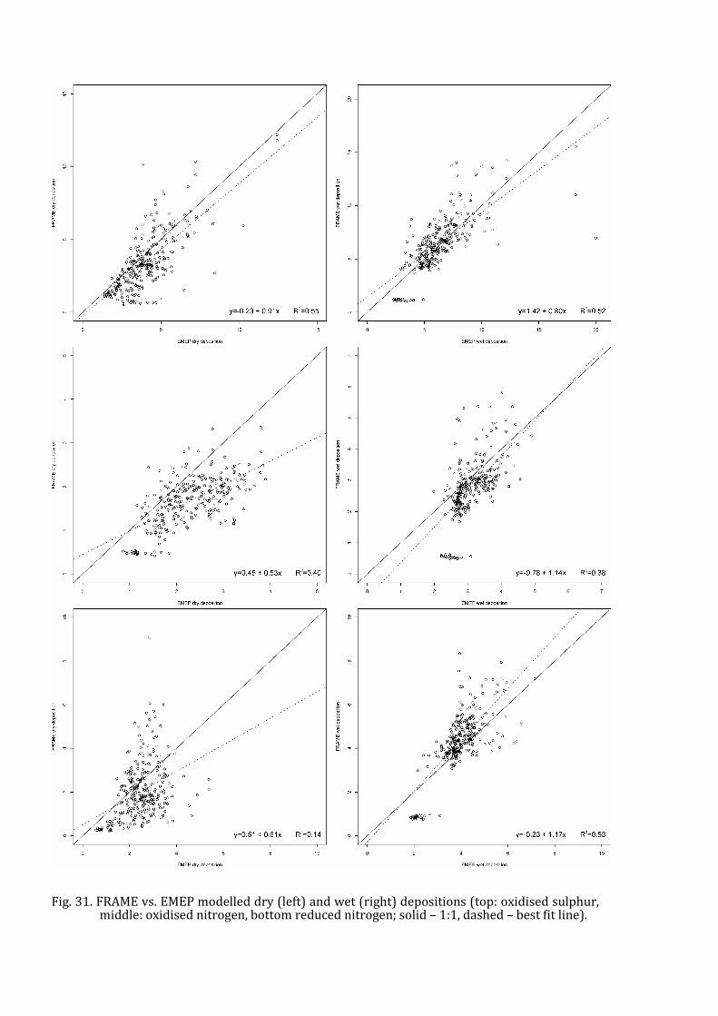
Fig. 31. FRAME vs. EMEP modelled dry (left) and wet (right) depositions (top: oxidised sulphur, middle: oxidised nitrogen, bottom reduced nitrogen; solid – 1:1, dashed – best fit line).

Fig. 32. Boxplots calculated from FRAME and EMEP estimates of oxidised sulphur (top), oxidised nitrogen (middle) and reduced (bottom) concentration (conc; μg•m-3) and dry and wet depositions (kg ha-1•y-1) for the area of Poland. Statistics are: minimum, 1st quartile, mean, 3rd quartile and maximum.

6.5. SUMMARY AND CONCLUSIONS

The spatial patterns of FRAME-PL modelled air concentration and depositions are in general agreement with the EMEP estimates. The main differences stem from the high resolution of FRAME-PL, which often leads to large variation of the modelled concentration or depositions within a single EMEP grid. This is especially important for reduced nitrogen, for which large local gradients in emission (and therefore in air concentration and dry depositions) are common. Model parameterization as well as emission inventory, both fill in the gaps in point sources database and improvements in spatial disaggregation of the area sources, are the fields of further improvements of the FRAME-PL model performance, despite the overall good agreement with the measurements. This includes especially the seeder-feeder process parameterization, which is currently based on long-term climatological data and has a large impact on estimated wet deposition, especially over mountainous areas. It was shown that e.g. Kasprowy Wierch station suffered from incorrect parameterization of the process.

Better quality of the emission inventory, preferably based on the bottom-up modelling approach, will certainly benefit the FRAME-PL performance in case of modelled air concentration and depositions. It should be stressed however that despite the simple approach used to calculate the spatial patterns of emission, there is a close agreement between modelled and measured values. It is also known that the bottom-up approach needs significantly larger amounts of input data, which are currently not available in Poland.

In general, the validation of the FRAME-PL model suffers from the limited number of monitoring sites, especially due to low

number of regional background sites and ammonia air concentration measurements. As the relative contribution of reduced nitrogen in acid and eutrophic deposition in Europe has been recently increasing, the number of monitoring sites is expected to be increased as well. This is not the case of Poland, where reduced nitrogen is not routinely measured within the frame of National Monitoring Programme. This is a surprising state of affairs, taking into account that Poland is among the countries emitting the largest quantities of NH3 in Europe. Furthermore, according to the current legislation, most of the monitoring sites for SO2 and NOx are located in the densely populated urban areas, therefore their usability for numerical model validation is limited.

The validation of the FRAME-PL model was performed for the year 2002 only. The results suggest that the model output is generally in reasonable or good agreement with the available measurements and with other models. The discrepancies may be partly explained by the fact, that the point measurements are compared with grid averaged estimates. However, to confirm the quality of the model results, the validation should be performed also for other years. This will make the conclusions more robust and meaningful.

The successful validation of the FRAME model suggests that the model can be considered as a suitable tool for calculating the concentration and deposition of nitrogen and sulphur compounds which can be used to estimate exceedance of critical loads for acid deposition and nitrogen deposition as well as critical levels for air concentration.

6.6. REFERENCES Aikawa, M., Hiraki, T., Tamaki, M., Shoga, M.,

2003. Difference between filtering-type bulk and wet-only data sets based on site classification. Atmospheric Environment 37, 2597-2603.

Allan, M.A., 2004, Manual for the gaw precipitation chemistry programme. Guidelines, Data Quality Objectives and Standard Operating Procedures. WMO TD no 1251.

Bjørge, D., Skålin, R., 1995, PARLAM - the parallel HIRLAM version at DNMI, Research Report No. 27, ISSN 0332-9879 Norwegian Meteorological Institute, Oslo, Norway.

Błaś, M., Dore, A.J., Sobik, M., 1999, Distribution of precipitation and wet deposition around an island mountain in south-west Poland. Quarterly Journal Royal Meteorological Society 125, 253-270.

Bush, T., King, K., Passant, N., Tsagatakis, I., 2008, NAEI UK emission maping methodology. NAEI.

Dore, A.J., Sobik, M., Migała, K., 1999, Patterns of precipitation and pollutant deposition in the Western Sudety Mountains, Poland. Atmospheric Environment 33, 3301-3312.

Dore, A.J., Theobald, M.R., Kryza, M., Vieno, M., Tand, S.Y., Sutton, M.A., 2007a, Modelling the deposition of reduced nitrogen at different scales in the United Kingdom. Proc. 29th NATO/SPS International Technical Meeting on Air Pollution Modelling and its Aplication, Aveiro, Portugal (in press).

Dore, A.J., Vieno, M., MacDougal, M., Kryza, M., Błaś, M., Hall, J., Dosio, A., Tang, S., Smith, R., Bealey, B., Sutton, M., 2007b, Modelling the deposition and concentration of long range air pollutants: final report. DEFRA pp. 87.

EMEP/CCC-Report 1/95, 2001, EMEP manual for sampling and chemical analysis. Norwegian Institute for Air Research.

Fagerli, H., Simpson, D., Tsyro, S., 2004, Transboundary acidification, eutrophication and ground level ozone in Europe, EMEP Status Report 1/2004, Unified EMEP model: Updates, The Norwegian Meteorological Institute, Oslo, Norway, 2004, pp. 11-18.

Goodison, B.E., Ferguson, H.L., McKay, G.A., 1981, Measurement and data analysis. [In:] Gray, D.M., Male, D.H. (eds.), Handbook of snow: Principles, Processes, Management and Use. Pergamon Press, Toronto, pp 776.

Hertel, O., Skjøth, C.A., Lofstrøm, P., Geels, C., Frohn, L.M., Ellermann, T., Madsen, P.V., 2006, Modelling nitrogen deposition on a local scale – a review of the current state of the art. Environmental Chemistry 3, 317-337.

Larson, L.W., Peck, E.L., 1974, Accuracy of precipitation measurements for hydrologic modeling. Water Resource Research 10 (4), 857-863.

Metcalfe, S.E., Whyatt, J.D., Broughton, R., Derwent, R.G., Finnegan, D., Hall, J., Mineter, M., O’Donougue, M., Sutton, M.A., 2001, Developing of the Hull Acid Rain Model: its

validation and implications for policy makers. Environmental Science & Policy 4, 25-37.

Metcalfe, S.E., Whyatt, J.D., Nicholson, J.P.G., Derwent, R.G., Heywood, E., 2005, Issues in model validation: assessing the performace of a regional-scale acid deposition model using measured and modelled data. Atmospheric Environment 39, 587-598.

Mol, W.J.A., Leeuw, F.A.A.M., 2005, AirBase: A Valuable Tool in Air Quality Assessments in: The Proceedings of the 5th International Conference on Urban Air Quality, Valencia, Spain 29-31 March 2005, Editors: Sokhi, R.S., Millán, M.M., Moussiopoulos, N.

Sandnes, L.H., Tsyro, S., 2000, Meteorological input data for EMEP/MSC-W air pollution models, EMEP MSC-W Note 2/2000.

Simpson, D., Fagerli, H., Jonson, J.E., Tsyro, S., Wind, P., Tuovinen, J.P., 2003, Transboundary acidification and eutrophication and ground level ozone in Europe: Unified EMEP Model Description, EMEP Status Report 1/2003 Part I, EMEP/MSC-W Report, The Norwegian Meteorological Institute, Oslo, Norway, 2003.

Skjøth, C.A., Hertel, O., Gyldenkaerne, S., Ellermann, T., 2004, Implementing a dynamical ammonia emission parametrization in the large-scale air pollution model ACDEP. Journal of Geophysical Research-Atmospheres, 109(D6), Art. No. D06306 MAR 23 2004.

Skotak, K., Iwanek, J., Mitosek, G., 2003, Ocena stanu zanieczyszczenia powietrza w Polsce w 2002 roku na podstawie pomiarów w sieci podstawowej. IOŚ Warszawa pp. 138,

Seinfeld, J.H., Pandis, S.N., 2006, Atmospheric chemistry and physic: From air pollution to climate change. Wiley Interscience.

Sofiev, M.A., 1999, Validation of model results on different scales. In: Bouwman A.F. (ed.), Approaches to scaling a trace gasflux in ecosystems, Elsevier.

Sornette, D., Davis, A.B., Ide, K., Vixie, K.R., Pisarenko, V., Kamm, J.R., 2007, Algorithm for model validation: Theory and applications. PNAS 104(16), 6562-6567.

Staelens, J., An De Schrijver, Van Avermaet, P., Genouw, G., Verhoest, N., 2005, A comparison of bulk and wet-only deposition at two adjacent sites in Melle (Belgium). Atmospheric Environment 39, 7-15.

Stedman, J.R., Heyes, C.J., Irwin, J.G., 1990, A comparison of bulk and wet-only precipitation collectors at rural sites in the United Kingdom. Water, Air, & Soil Pollution 52, 377–395.

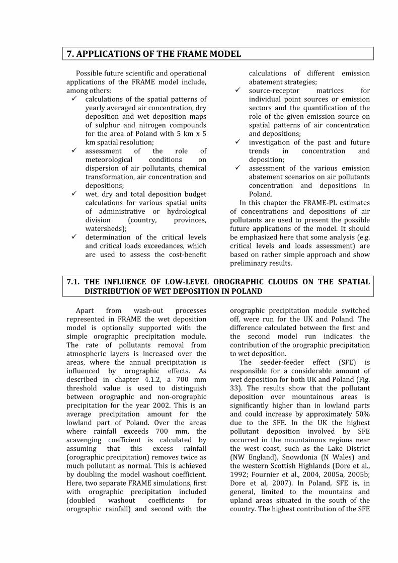
7. APPLICATIONS OF THE FRAME MODEL

Possible future scientific and operational applications of the FRAME model include, among others: � calculations of the spatial patterns of

yearly averaged air concentration, dry deposition and wet deposition maps of sulphur and nitrogen compounds for the area of Poland with 5 km x 5 km spatial resolution;

� assessment of the role of meteorological conditions on dispersion of air pollutants, chemical transformation, air concentration and depositions;

� wet, dry and total deposition budget calculations for various spatial units of administrative or hydrological division (country, provinces, watersheds);

� determination of the critical levels and critical loads exceedances, which are used to assess the cost-benefit

calculations of different emission abatement strategies;

� source-receptor matrices for individual point sources or emission sectors and the quantification of the role of the given emission source on spatial patterns of air concentration and depositions;

� investigation of the past and future trends in concentration and deposition;

� assessment of the various emission abatement scenarios on air pollutants concentration and depositions in Poland.

In this chapter the FRAME-PL estimates of concentrations and depositions of air pollutants are used to present the possible future applications of the model. It should be emphasized here that some analysis (e.g. critical levels and loads assessment) are based on rather simple approach and show preliminary results.

7.1. THE INFLUENCE OF LOW-LEVEL OROGRAPHIC CLOUDS ON THE SPATIAL DISTRIBUTION OF WET DEPOSITION IN POLAND

Apart from wash-out processes

represented in FRAME the wet deposition model is optionally supported with the simple orographic precipitation module. The rate of pollutants removal from atmospheric layers is increased over the areas, where the annual precipitation is influenced by orographic effects. As described in chapter 4.1.2, a 700 mm threshold value is used to distinguish between orographic and non-orographic precipitation for the year 2002. This is an average precipitation amount for the lowland part of Poland. Over the areas where rainfall exceeds 700 mm, the scavenging coefficient is calculated by assuming that this excess rainfall (orographic precipitation) removes twice as much pollutant as normal. This is achieved by doubling the model washout coefficient. Here, two separate FRAME simulations, first with orographic precipitation included (doubled washout coefficients for orographic rainfall) and second with the

orographic precipitation module switched off, were run for the UK and Poland. The difference calculated between the first and the second model run indicates the contribution of the orographic precipitation to wet deposition.

The seeder-feeder effect (SFE) is responsible for a considerable amount of wet deposition for both UK and Poland (Fig. 33). The results show that the pollutant deposition over mountainous areas is significantly higher than in lowland parts and could increase by approximately 50% due to the SFE. In the UK the highest pollutant deposition involved by SFE occurred in the mountainous regions near the west coast, such as the Lake District (NW England), Snowdonia (N Wales) and the western Scottish Highlands (Dore et al., 1992; Fournier et al., 2004, 2005a, 2005b; Dore et al, 2007). In Poland, SFE is, in general, limited to the mountains and upland areas situated in the south of the country. The highest contribution of the SFE

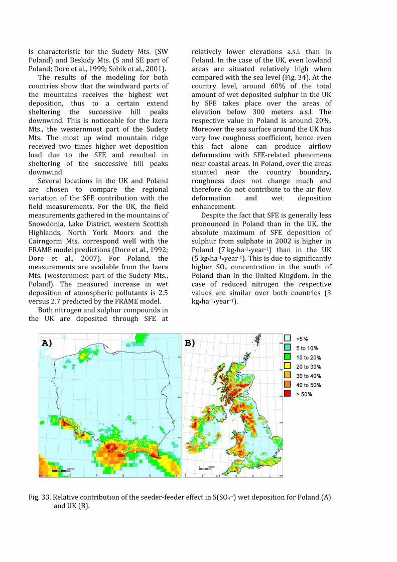
is characteristic for the Sudety Mts. (SW Poland) and Beskidy Mts. (S and SE part of Poland; Dore et al., 1999; Sobik et al., 2001).

The results of the modeling for both countries show that the windward parts of the mountains receives the highest wet deposition, thus to a certain extend sheltering the successive hill peaks downwind. This is noticeable for the Izera Mts., the westernmost part of the Sudety Mts. The most up wind mountain ridge received two times higher wet deposition load due to the SFE and resulted in sheltering of the successive hill peaks downwind.

Several locations in the UK and Poland are chosen to compare the regional variation of the SFE contribution with the field measurements. For the UK, the field measurements gathered in the mountains of Snowdonia, Lake District, western Scottish Highlands, North York Moors and the Cairngorm Mts. correspond well with the FRAME model predictions (Dore et al., 1992; Dore et al., 2007). For Poland, the measurements are available from the Izera Mts. (westernmost part of the Sudety Mts., Poland). The measured increase in wet deposition of atmospheric pollutants is 2.5 versus 2.7 predicted by the FRAME model.

Both nitrogen and sulphur compounds in the UK are deposited through SFE at

relatively lower elevations a.s.l. than in Poland. In the case of the UK, even lowland areas are situated relatively high when compared with the sea level (Fig. 34). At the country level, around 60% of the total amount of wet deposited sulphur in the UK by SFE takes place over the areas of elevation below 300 meters a.s.l. The respective value in Poland is around 20%. Moreover the sea surface around the UK has very low roughness coefficient, hence even this fact alone can produce airflow deformation with SFE-related phenomena near coastal areas. In Poland, over the areas situated near the country boundary, roughness does not change much and therefore do not contribute to the air flow deformation and wet deposition enhancement.

Despite the fact that SFE is generally less pronounced in Poland than in the UK, the absolute maximum of SFE deposition of sulphur from sulphate in 2002 is higher in Poland (7 kg•ha-1•year-1) than in the UK (5 kg•ha-1•year-1). This is due to significantly higher SOx concentration in the south of Poland than in the United Kingdom. In the case of reduced nitrogen the respective values are similar over both countries (3 kg•ha-1•year-1).

Fig. 33. Relative contribution of the seeder-feeder effect in S(SO4--) wet deposition for Poland (A) and UK (B).

Fig. 34. Cumulative contribution of the seeder- feeder effect (CSFC) in S(SO4--) wet deposition for Poland and UK (lines) versus height above sea level (bars); (RHC [%] – percentage contribution of area in 100 m height resolution).

7.2. EXCEEDANCES OF CRITICAL LOADS AND LEVELS 7.2.1. Introduction

Critical level and loads are defined as a quantitative estimate of an exposure to one or more pollutants below which significant harmful effects on specified sensitive elements of the environment do not occur according to present knowledge (Nilsson and Grenfelt, 1988). Critical level (CLev) refers to the air concentration of atmospheric pollutant above which direct adverse effects on receptors, such as human beings, plants, ecosystems or materials may occur (UNECE, 1999). Critical loads (CL) refer to the amount of atmospheric pollutant depositions that receptor can tolerate without negative effects. CLev and CL are the basis for policies controlling emission of acidifying and eutrophying substances in Europe and elsewhere (UNECE, 1999). Depositions and air pollutants concentrations which are above the specified critical load or level are known as “exceedances”, and the aim of emission control policies is to reduce and, if possible, to eliminate the areas with exceedances within a given timescale. Every exceedance of critical loads of acidity or eutrophication may cause adverse effects to ecosystems in

the long-term, resulting in various environmental disturbances. Depending on the degree of acidification or eutrophication, these disturbances can vary from e.g. slightly changed health status of some most vulnerable species to the complete die-back of the predominant one.

The critical load and level concepts have been developed since the 1980s under the UNECE Convention on Long-range Transboundary Air Pollution, providing an important reference point against which pollution levels can be compared. Often the values of the model input parameters are poorly known, either because they are difficult to measure, or because they are estimated from national data base rather than site specific measurements, or because they are intrinsically, spatially or temporally variable (Skeffington et al., 2007). There are numerous studies dealing with uncertainty in estimation of critical loads and levels (e.g. Hettelingh and Jansen, 1993; Barkman and Alveteg, 2001; Suutari et al., 2001; UBA, 2004; Van Dobben et al., 2006; Sutton et al., 2006; Sutton, 2009).

CLev and CL can be used for calculating emission ceilings for individual countries with respect to acceptable air pollution levels (UBA, 2004). For Poland, maps of critical loads of acidity and eutrophication have been produced since 1991. For the assessment of the exceedances, the maps of critical loads are usually combined with the EMEP-Unified model result (50 km x 50 km grid; Mill et al., 2005; Mill, 2006). In the United Kingdom, exceedances of the CL are calculated with higher spatial resolution, with sulphur and nitrogen deposition data modelled with the use of FRAME and CBED

models, to provide the necessary input information on deposition (Hall et al., 2006).

This study presents preliminary results of the assessment of the exceedances of the CLev and CL exceedance for the semi-natural ecosystems in Poland on the basis of a high-resolution long-range transport model – FRAME with 5 km x 5 km resolution. The exceedances calculated with the FRAME modelled deposition are compared with the results based on the EMEP data. This is performed to assess the role of the model spatial resolution on the assessment of the CL exceedances.

7.2.2. Exceedance estimates

Due to a lack of data and the preliminary form of the study, a simple approach was chosen, based on empirical critical loads/levels proposed by UBA (2004). The exceedance Ex(Xdep/conc) of the critical load/level CL(Xdep/conc) is given as:

Ex(Xdep/conc)=Xdep/conc – CL(Xdep/conc)

where:

Xdep/conc – deposition (dep) or concentration (conc) of a pollutant X.

If the Xdep/conc>CL(Xdep/conc), the critical

load or level is exceeded, and the amount of

the exceedance is marked on the presented maps. The critical levels for yearly average concentration of SO2, NO2 were set, after UBA (2004), to 20 and 30 μg•m-3, respectively. The critical level of NH3 was set to 3 μg•m-3 according to Sutton (2009). The critical loads for many ecosystems are currently estimated within the range 10-15 kg N ha-1•y-1 (UBA, 2004). Here, the threshold of 10 kg N ha-1•y-1 was chosen. The forest and semi-natural areas were selected based on the CORINE Land Cover database.

7.2.3. Results

According to the FRAME and EMEP model estimates with methodology suggested by UBA (2004), the critical level of SO2 is not exceeded for the semi-natural surfaces in Poland. There are small areas where the NO2 critical load is exceeded and they are mainly located in the close vicinity of large cities and main roads. Although spatially not extensive, the exceedances of the NO2 critical loads are in some regions significant.

The total extent of the semi-natural areas where the critical level for ammonia is exceeded according to the FRAME model surpasses 6000 km2 (Fig. 35). The majority of the areas with CL exceeded are located in the central part of Poland, where NH3 emission is high due to intensive

agricultural production. The exceedances are usually lower than 2.5 μg·m-3, but locally reach 5.0 μg·m-3. For the EMEP model, the total extent of the area with the exceedance of the NH3 critical level is substantially smaller than estimated with FRAME and the exceedances are not larger than 2.5 μg·m-3 (Tab. 6). Within the 0-2.5 μg·m-3 span most of the grids have the exceedance below 0.5 μg·m-3.

The critical load for the total atmospheric nitrogen deposition (oxidised and reduced nitrogen) is exceeded, according to FRAME deposition estimates, for almost 90% of the semi-natural areas in Poland. Over the mountainous areas to the south, the exceedances are locally over 10 kg N ha-1•y-1 (Fig. 36; Tab. 6). The exceedances are also

significant in the central part of Poland, where high emission of NH3 due to the intensive agriculture and large dry deposition of NHx close to the emission sources take place. EMEP modelled deposition of nitrogen gives lower

exceedances than calculated with the FRAME deposition data, with the exception of the western parts of Poland. This is a result of advection of the polluted air from foreign west-European sources in the prevailing westerly wind condition.

Tab. 6. Total areas [km-2] with the critical level (NOx, NH3 [μg•m-3•y-1]) and loads CL (total N, [kg N ha-1•y-1]) exceeded.

NOx NH3 Total N

CLev, CL FRAME EMEP FRAME EMEP FRAME EMEP

No exceedance 94884 95062 88729 94091 11508 4283 0-2.5 79 0 5872 971 47819 42965

2.5-5.0 30 0 429 0 26316 40500 5.0-10.0 37 0 32 0 8030 7314

>10.0 32 0 0 0 1389 0 Total: 95062 95062 95062 95062 95062 95062

Fig. 35. The exceedance of the critical level of NH3 [μg⋅m-3] based on the FRAME model.

Fig 36. The exceedance of the critical load for the total atmospheric nitrogen deposition [kg⋅ha-1⋅y-1] based on the FRAME model.

The preliminary results of the

assessment of the exceedances of the critical levels and loads show that the FRAME model can be useful in this kind of study supporting the national strategies on emission abatements and environmental protection. The FRAME-EMEP comparison shows that the decisions based on deposition data calculated with these models may differ significantly. In general, the high resolution of the FRAME model results in locally higher air concentration and depositions, which are averaged out

over 50 km x 50 km EMEP grid. This affects the critical levels and loads assessment and may result in insufficient protection of the various ecosystems against acidification and eutrophication caused by sulphur and nitrogen deposition. It should be noticed that the calculations presented here are based on a simplified approach, as no spatial information on the critical load were available for the authors. Because of the simplifications assumed in this work, the critical levels and loads should be further investigated.

7.3. SOURCE–RECEPTOR ANALYSIS

Because of the relatively short calculation time, FRAME can be considered as a useful tool for source-receptor calculations, often used in Integrated Assessment Modelling to assess the influence of individual emission sources on air concentration and depositions. This

procedure can be used to estimate the most cost effective strategy of protecting the environment from the effects of air pollution by reduction of emission (Samson et al., 1986; Mediavilla-Sahagún et al., 2002; Oxley et al., 2003; Warren and ApSimon, 2004). Air concentration or deposition

footprint of the given emission source can be calculated with FRAME by running two model simulations: the first one with all emission included; the second with a given single source or a given group of sources removed (e.g. point source or emission sector). The footprint (or source-receptor matrix) is the difference in deposition or concentration between the first and second simulations. Fig. 37 presents the total deposition of sulphur in 2002 from a single source with the Turów Power Plant (SW Poland) as an example. Due to the high wind frequency from the SW-W as well as an enhanced washout rate over westernmost parts of the Izera Mts., the highest deposition is located mainly over the westernmost part of the Sudety Mts.

Another example show the influence of national emission and the transboundary contribution on deposition of reduced nitrogen in Poland for 2002 (Fig. 38). Two FRAME simulations were undertaken, one (base simulation) with the emission data from Poland and surrounding countries, as well as boundary concentration (transboundary transport of pollutants) calculated with FRAME-Europe (50km x 50km) included. For the second simulation,

only the Poland domestic emission sources are considered and boundary concentration is set to zero. The resultant map, show the difference between the base (all sources included) and second (PL-only emission) simulation, given as the fraction of reduced nitrogen deposition from transboundary contribution are visible (Fig. 38). The source attribution analysis, performed with the FRAME model, shows that national emission of NH3 is responsible for almost 64% of total deposition of reduced nitrogen in Poland, which is close to EMEP estimates (58%; Jonson et al., 1998; Klein et al, 2004). According to FRAME estimates, up to 93% of dry deposition in Poland comes from national activities, while the transboundary contribution reaches 53% of wet deposition. The western part of Poland and the mountainous areas in the south are strongly influenced by the deposition of reduced nitrogen from transboundary transport. In the mountains, due to prevailing westerly wind conditions, over 80% (locally over 90%) of the total NHx deposition comes from sources located outside of Poland. Similar spatial patterns, calculated with the EMEP model, were earlier presented by Klein et al. (2004).

Fig. 37. Total deposition of sulphur emitted from the Turów Power Plant (SW Poland).

Fig. 38. Transboundary contribution to total reduced nitrogen deposition in Poland.

The presented here list of examples of applications of FRAME data for various environmental studies is not complete and there exists large further potential for the model application in air quality management at regional and local scale.

This is particularly the case of combined source – receptor with critical level and loads exceedances analysis. This kind of integrated approach can efficiently support the environmental policy in Poland.

7.4. REFERENCES Barkman, A., Alveteg, M., 2001, Effects of data

uncertainty in the Swedish critical load assessment for forest soils. Water, Air & Soil Pollution 125, 133-156.

Dore, A.J., Choularton, T.W., Fowler, D., 1992, An improved wet deposition map of the United Kingdom incorporating the topographic dependence of rainfall concentrations. Atmospheric Environment 26A, 1375-1381.

Dore, A.J., Sobik, M., Migała, K., 1999, Patterns of precipitation and pollutant deposition in the Western Sudety Mountains, Poland. Atmospheric Environment 33, 3301-3312.

Dore, A.J., Vieno, M., Tang, Y.S., Dragosits, U., Dosio, A., Weston, K.J., Sutton, M.A., 2007, Modelling the atmospheric transport and deposition of sulphur and nitrogen over the

United Kingdom and assessment of the influence of SO2 emissions from international shipping, Atmospheric Environment 41, 2355-2367.

Fournier, N., Dore, A.J., Vieno, M., Weston, K.J.W., Dragosits. U., Sutton, M.A., 2004, Modelling the deposition of atmospheric oxidised nitrogen and sulphur to the United Kingdom using a multi-layer long-range transport model. Atmospheric Environment 38(5), 683-694.

Fournier, N., Weston, K.J.W., Dore, A.J., Sutton, M.A., 2005a, Modelling the wet deposition of reduced nitrogen over the British Isles using a multi-layer atmospheric transport model. Quarterly Journal of the Royal Meteorological Society 131, 703-722.

Fournier, N., Tang, Y.S., Dragisits, U., Kluizenaar, Y., Sutton, M.A., 2005b, Regional atmospheric budgets of reduced nitrogen over the British Isles assessed using a multi-layer atmospheric transport model. Water, Air & Soil Pollution 162, 331-351.

Hall, J., Dore, A.J., Heywood, E., Broughton, R., Stedman, J., Smith, R.I., Hanlon, S.O., 2006, Assessment of the environmental impacts associated with the UK Air Quality Strategy. Report to DEFRA. http://www.airquality.co.uk/archive/reports/

Hettelingh, J-P., Jansen, P., 1993, Preliminary uncertainty and sensitivity analysis of computed critical deposition in Europe. [In:] Downing, R.J., Hettelingh, J-P., de Smet PAM (eds), Calculation and mapping of critical loads in Europe: status report 1993. Bilthoven, The Niederlands: RIVM.

Jonson, J.E., Bartnicki, J., Olendrzyński, K., Jakobsen, H.A., Berle, E., 1998, EMEP Eulerian model for atmospheric transport and deposition of nitrogen species over Europe. Environmental Pollution 102(S1), 289-298.

Klein, H., Wind, P., van Loon, M., 2004, Transboundary air pollution by main pollutants (S, N, O3) and PM: Poland. MSC-W Data Note 1/2004.

Mediavilla-Sahagún, A., ApSimon, H.M., Warren, R.F., 2002, Integrated assessment of abatement strategies to improve air quality in urban environments, the USIAM Model, Water, Air & Soil Pollution, Vol. 2 (5-6), 689-701.

Mill, W., Schlama, A., Kacprzyk, W., 2005, Polish National Ocal Centre Report. [In:] Posch, M., Slootweg, J., Hettelingh, J.-P. (eds.), European critical loads and dynamic modelling: CCE Status Report 2005. Netherlands Environmental Assessment Agency, Bilthoven, The Netherlands, 135-140.

Mill, W., 2006, Temporal and spatial development of critical loads exceedance of acidity to Polish forest ecosystems in view of economic transformations and national environmental policy. Environmental Science & Policy 9, 563-567.

Nilsson, J., Grennfelt, P., 1988, Critical loads for sulphur and nitrogen 1988:15. Copenhagen: Nordic Council of Ministers.

Oxley, T., ApSimon, H., Dore, A.J., Sutton, M.A. Hall, J., Heywood, E., Gonzales del Campo, T., Warren, R., 2003, The UK Integrated Assessment Model, UKIAM: A National Scale Approach to the analysis of strategies for abatement of atmospheric pollutants under

the convention on long-range transboundary air pollution, Integrated Assessment 4, 236-249.

Samson, P.J., Fernau, M., Allison, P., 1986, On the variability of simulated source-receptor relationships for sulphur deposition. Water, Air & Soil Pollution 30, 801-813.

Skeffington, R.A., Whitehead, P.G., Heywood, E., Hall, J.R., Wadsworth, R.A., Reynolds, B., 2007, Estimating uncertainty in terrestrial critical loads and their exceedance at four sites in the UK. Science of the Total Environment 382, 199-213.

Sobik, M., Netzel, P., Quiel, F., 2001, Zastosowanie modelu rastrowego do określenia pola rocznej sumy opadów atmosferycznych na Dolnym Śląsku. Rocznik Fizyczno-Geograficzny, VI, 27-34.

Sutton, M., Sheppard, L., Fowler, D., 2006, Potential for the further development and application of critical levels to assess the environmental impact of ammonia, Background Document of the Working Group 1, Expert Group on Ammonia Abatement, Edinburgh Workshop 2006.

Sutton, M.A., 2009, Introduction. [In:] Sutton, M.A., Reis, S., Baker, S.M.H., Atmospheric ammonia: detecting emission changes and environmental impacts, Springer.

Suutari, R., Amann, M., Cofala, J., Klimont, Z., Posch, M., Schöpp, W., 2001, From economic activities to ecosystem protection in Europe. An uncertainty analysis of the RAINS integrated assessment model. Luxemburg, Austria: IIASA.

UBA, 2004, Manual on methodologies and criteria for modelling and mapping of critical loads and levels and air pollution effects, risk and trends, UBA-Texte 52/2004.

UNECE. Protocol to abate acidification, eutrophication and groundlevel ozone. Geneva: UNECE; 1999 www.unece.org/env/1rtap/multi_h1.htm.

Van Dobben, H.F., Van Hinsberg, A., Schouwenberg, E.P.A.G., Jansen, M., Mol-Dijkstra, J.P., Wieggers, H.J.J., et al., 2006, Simulation of critical loads for nitrogen for terrestrial plant communities in The Niederlands. Ecosystems 9; 32-45.

Warren, R., ApSimon, H., 2004, Integrated Assessment modelling of abatement strategies: Role of uncertainties. Air Pollution Modelling and Its Application XIV, 35-44.

8. FACTORS CONTROLLING DEPOSITION PROCESSES IN DIFFERENT SCALES

Meteorological factors are crucial for

controlling the spatial and temporal distribution of both the concentration and deposition of atmospheric pollution. The analysis of atmospheric pollution dispersion, transport and removal processes, including physical and chemical transformations of pollutants, is an essential condition to explain the relationships between emission, concentration and deposition levels. After being transported and transformed, pollutants are deposited on a surface by dry and wet deposition. The latter component is completed by cloud or fog deposition, which shall be understand as direct transfer of cloud or fog droplets to the ground surface, with all dissolved and suspended substances.

Pollutant deposition shows a large spatial variability at various spatial scales. Orlanski (1975) proposed a set of scales for atmospheric processes which have an influence on spatial distribution of deposition rate. Meso-scale has an extension of up to several hundred kilometers and is characterized by progression of air-masses. Topo-scale is a function of slope, aspect and topographic position (ridge to valley). The term micro-scale or micro-climate is often applied to spatial scales up to 1 km (Orlanski, 1975). Microclimate is a function of vegetation canopy structure and mainly associated with processes in the surface layer.

FRAME model is accurate to show meso- and topo-scale factors influencing spatial distribution of concentration and pollutant deposition.

8.1. ATMOSPHERIC CIRCULATION – THE ROLE OF THE MESO-SCALE CONDITIONS ON AIR POLLUTANTS CONCENTRATION AND DEPOSITION

Atmospheric pollutants, due to long-

range transport, can affect distant regions, even those several hundred kilometres away from pollution sources (Erisman and Draaijers, 1995). It is caused by various factors, including air mass origin and transformation, synoptic conditions, transport velocity, thermal stratification, depth of atmospheric boundary layer, as well as technical parameters of the emission source (i.e. effective height of the emission). Atmospheric processes can preserve pollution in steady state for a relatively long

time, or can trigger fast removal of pollutants to the ground. The effective removal of air pollutants is caused by chemical liquid-phase transformations in clouds (Hegg and Hobbs, 1981; Radojevic et al., 1995) and by water flux from the atmosphere to the ground in the form of precipitation and horizontal precipitation (deposition of the fog droplets; Baron and Sobik, 1995; Weathers et al., 1995; Sobik, 1999; Tesař et al., 2000; Błaś, 2001; Weathers et. al., 2006).

8.2. TOPO–CLIMATIC FACTORS AND AIR POLLUTANTS CONCENTRATION AND DEPOSITION

Topo-climatic scale effects were examined in the Sudety Mts., which, similarly to many other middle-size mountain ranges in Europe, are seriously affected by atmospheric pollutant deposition. During typical westerly wind conditions the mountain range is well

exposed to the inflow of highly polluted air from the areas of heavy industry, concentrated at the distance of tens to hundreds of kilometres on the windward side of the mountains. One of the atmospheric processes leading to precipitation formation or a regional

enhancement of already existing precipitation is an ascent of sufficiently humid air masses forced by the morphology of a mountain barrier. Such an effect is visible, e.g., in the Sudety Mts., where annual precipitation sums are typically 50-150% higher than in the surrounding lowlands (Dore et al., 1999; Błaś, 2001; Sobik et al., 2001).

Except for the role of a mountain barrier as a whole, some local effects in topo-scale are visible. The first one is the "seeder-feeder" effect – which causes precipitation enhancement on mountain summits and ridges due to raindrops (or snowflakes) growth when they cross a low level orographic cap-cloud which is frequently formed over mountain tops (see chapter 4.1.3 and Figure 8; Bergeron, 1965; Choularton et. al., 1988). Such orographic processes observed in the Sudety Mts., if compared with the surrounding lowland

terrain, typically results in doubling of rainfall and even tripling the pollutant deposition (Błaś et al., 1999; Dore et al., 1999). Long-term monitoring studies show that the highest deposition has been observed on the windward slope of the first orographic barrier of the Sudety Mts. (Błaś, 2001; Dore et al., 1990). The second important topo-scale effect influencing the concentration and deposition of atmospheric pollutants is fog deposition which vary considerably from site to site and depends, among others, on altitude, aspect, the relative height of a windward slope, the screening effect of surrounding relief, etc. (Błaś, 2001; Sobik et. al., 1998). It has been observed that the highest potential efficiency of horizontal precipitation is typical for high elevated slopes and ridges exposed to maritime air masses with lowlands at the windward side.

8.3. MICROSCALE FACTORS AND AIR POLLUTANTS CONCENTRATION AND DEPOSITION

Roughness, characteristic for particular types of landuse, is the most important factor responsible for the significant differentiation of dry and wet deposition of pollutants in a micro-scale. The efficiency of non precipitation atmospheric deposits (e.g. fog, dew and hoarfrost, see also chapter 9) depend on the size and surface area of any receptor present (rocks, grass, dwarf pine, forest etc.).

In a mountainous terrain vegetation has important influence on the hydrological and chemical flux. Particularly in forested areas where it efficiently intercepts fog droplets, as an example. Considering the height and surface area index (SAI), the highest efficiency of horizontal precipitation is characteristic for spruce trees which are the most common in the Sudety Mts. Fog precipitation rate can change considerably over short distances because of a different tree height, structure and size, and the frequency of gaps in the forest canopy (Weathers et. al., 1995 and 2006; Sobik et. al., 1998). A well exposed tree can receive a

few times more deposition than another one of equivalent SAI and height that is sheltered by its neighbours. It should be taken into account that land use changes caused by human activity modify an existing field of pollutant deposition. For example, as a result of clearcuts of mountain forests, the pollutant deposition field in the Karkonosze Mts. can be significantly altered with the maxima of deposition rate at newly exposed forest edges. This can lead to the critical loads exceedances, even if abatements in emission rates at national or international scale are noted and regional ATMs, like FRAME and EMEP, suggest overall decrease in deposition of acidifying and eutrhopic pollutants.

Meadows are the areas well disposed for dew or hoarfrost deposition. Lower intensity of dew or hoarfrost is characteristic for arable lands and forests while at urban areas dew or hoarfrost are relatively rare phenomena and form with the weakest efficiency.

8.4. REFERENCES

Baron, H., Sobik, M., 1995, Rola osadów atmosferycznych w zakwaszaniu środowiska przyrodniczego wierzchowiny Karkonoszy. Acta Univesitatis Wratislaviensis, Prace Instytutu Geograficznego, Seria C. Meteorologia i Klimatologia 1705, 59-73.

Bergeron, T., 1965, On the low level redistribution of atmospheric water caused by orography. [In:] Proceedings of the International Conference on Cloud Physics, Tokyo, May 1965, 96-100.

Błaś, M., Dore, A.J., Sobik, M., 1999, Distribution of precipitation and wet deposition around an island mountain in south-west Poland. Quarterly Journal of the Royal Meteorological Society 125, 253-270.

Błaś, M., 2001, Rola mgły w przychodzie wody i mokrej depozycji zanieczyszczeń w Sudetach. Unpublished Ph.D. Thesis, Wrocław, University of Wrocław.

Choularton, T.W., Gay, M.J., Jones, A., Fowler, D., Cape, J.N., Leith, I.D., 1988, The influence of altitude on wet deposition comparison between field measurement at Great Dun Fell and the predictions of a seeder-feeder model. Atmospheric Environment 22 (7), 1363-1371.

Dore, A.J., Choularton, T.W., Fowler, D., Storton-West, R., 1990, Field measurement of wet deposition in an extended region of complex topography. Quarterly Journal of the Royal Meteorological Society 116, 1193-1212.

Dore, A.J., Sobik, M., Migała, K., 1999, Patterns of precipitation and pollutant deposition by rain and snow in the western Sudety Mountains, Poland. Atmospheric Environment 33, 3301-3312.

Erisman, J.W., Draaijers, G. P. J., 1995, Atmospheric deposition in relation to acidification. Studies in Environmental Science, Elsevier.

Hegg, D.A., Hobbs, P.V., 1981, Cloud water chemistry and the production of sulfates in clouds. Atmospheric Environment 15, 1597-1604.

Orlanski, I., 1975, A rational subdivision of scales for atmospheric processes. Bull. Amer. Meteor. Soc. 56, 527–530.

Radojevic, M., Tyler, B.J., Hall, S., Penderghest, N., 1995, Air oxidation of S(IV) in cloud-water samples. Water, Air and Soil Pollution 85 (3/4), 1985-1990.

Sobik, M., Błaś, M., Quiel, F., 1998, Udział osadów mgielnych w przychodzie wody z atmosfery i depozycji zanieczyszczeń w lasach Sudetów Zachodnich. [In:] “Geoekologiczne Problemy Karkonoszy" - Materiały z sesji naukowej w Przesiece 15-18.X.1997, Poznań, 151-162.

Sobik, M., 1999, Meteorologiczne uwarunkowania zakwaszenia hydrometeorów w Karkonoszach. Maszynopis pracy doktorskiej, Wrocław, Uniwersytet Wrocławski, Instytut Geograficzny, Zakład Meteorologii i Klimatologii.

Sobik, M., Netzel, P., Quiel, F., 2001, Zastosowanie modelu rastrowego do określenia pola rocznej sumy opadów atmosferycznych na Dolnym Śląsku. Rocznik Fizyczno-Geograficzny, VI, 27-34.

Tesař, M., Fottová, D., Eliáš, V., Šír, M., 2000, Occult precipitation as an important contribution in Bohemian Forest. Silva Gabreta 4, 87-96.

Weathers, K.C., Lovett, G., Likens, G., 1995, Cloud deposition to a spruce forest edge. Atmospheric Environment 29, 665-672.

Weathers, K.C., Simkin, S.M., Lovett, G.M., Lindberg, S.E., 2006, Empirical modelling of atmospheric deposition in mountainous landscapes. Empirical modelling of atmospheric deposition in mountainous landscapes. Ecological Applications 16, 1590-1607.

9. NON PRECIPITATION ATMOSPHERIC DEPOSITS

9.1. INTRODUCTION

Non-precipitation atmospheric deposits i.e. fog, dew and hoarfrost form an important water flux from the atmosphere to the ground. Due to high concentration of chemical constituents they are particularly important in pollutant deposition processes. The chemical composition of dew and hoarfrost and fog water differs significantly from each other and from precipitation, and depends on emission character and atmospheric processes involved. Over the large areas of European lowlands dew and hoarfrost form an important path for pollutant flux to the ground enhancing by around 50% wet deposition carried via atmospheric precipitation. Pollutant

deposition via orographic fog is locally responsible for numerous deposition hot spots and frequent critical load exceedance and, as a contributing factor, for nowadays adverse effects currently visible in mountain forest ecosystems.

Current chapter shows the reason why one should carefully interpret the results of total deposition modelling, especially produced by low spatial resolution models. Even large scale modelling can not effectively include non-precipitation components of wet deposition because of their high spatial variability produced by local land morphology and very diversified pattern of land cover categories.

9.2. METEOROLOGICAL INTERPRETATION

9.2.1. Fog deposition Fog or clouds consists of a specific type

of atmospheric phenomena. Results obtained on the basis of analysis of suitable fog samples can be treated as a source of information on the chemistry of the atmosphere. Statistical analysis revealed significant differences depending on region, altitude, local morphology and, last but not least, fog origin. Clouds and fog play an important role as processors of atmospheric aerosols and soluble gases. Of particular interest are the roles they play in new particle production (e.g. via aqueous oxidation) and particle removal (e.g. via particle scavenging and removal by fog drop deposition or precipitation; Collett et al., 2002; Dore et al., 1999).

Fog precipitation (called also horizontal precipitation) is defined as the direct water flux of fog or cloud water droplets to the ground surface. Horizontal precipitation occurs when droplets, in the result of inertial impact, hit the surface of the receptor. The impact occurs when wind driven droplets travel along trajectories more or less parallel to the ground surface, which is typical for orographic (slope) fog.

Direct deposition of fog droplets to vegetation can also make an important additional contribution to chemical input. Finally, chemical composition of fog and cloudwater in particular is a sensitive indicator of emission patterns. For this reason, over the past decade, the chemical compositions of fog and clouds have been investigated in many places all over the world (Ferrier et al., 1995; Minami and Ishizaka, 1996; Acker et al., 1998; Puxbaum and Tscherwenka, 1998; Fišák and Řezáčová, 2001; Collett et al., 2002; Fišák et al., 2004; Błaś et al., 2008).

Monitoring cloud and fog chemistry could be a useful tool for complementary interpretation and identification of long range transport of air pollutants. The reasons are as follows: � on the basis of long term measurements

at the Szrenica Mt. the aggregated duration of precipitation equals only a dozen percent of total time (11-13% in individual years). In the case of fog, it is approximately 45% on average, which gives much longer lasting opportunity to control atmospheric chemistry (Archive

of the Meteorological Observatory of the Wrocław University);

� due to the more polluted nature of the boundary layer than the free atmosphere, fog water (originating in low-level air) have higher pollutant concentration than precipitation, therefore, cloud chemistry can be a more sensitive indicator of the

composition of regional emission than precipitation itself;

� clouds are a primary source of precipitation chemical composition;

� fog chemistry is a useful source of information about the long range transport of air pollutants in the case of lack of precipitation and absence of measurements of pollutant concentration in air.

9.2.2. Dew and hoarfrost

Except for dry, precipitation and fog induced deposition, there also exist other pathways of atmospheric pollutants flux into the ground. These are different kinds of atmospheric deposits in the form of hydrometeors, which do not belong to previously discussed fog deposition category i.e. dew and hoarfrost. Due to the lack of methodical standards concerning sampling and measurements of atmospheric deposits, the role of dew and hoarfrost in both water balance and pollutants deposition is often neglected (Muselli et al., 2002; Weathers et al., 2006; Polkowska and Sobik, 2008).

Dew is the product of direct condensation of atmospheric water vapour on the ground, the temperature of which has fallen below dew point but not below water freezing point. Examination of dew formation in microscale shows that different processes are involved in the growth of dew drops: direct accommodation at the drop surface in areas of maximum temperature gradients, nucleation and evaporation of clusters of near critical radius and coalescence of airborne small droplets formed earlier through nucleation (Beysens,

1995). Hoarfrost is similar in origin but is formed through ice crystals sublimation from water vapour when the temperature drops below freezing point.

In general both dew and hoarfrost are surface dependent and are formed as the result of surface cooling due to the negative thermal balance, which regularly takes place during calm and cloudless nights. Energy is emitted from any surface which contacts with the atmosphere, but only objects with low thermal conductivity are cooled significantly below the dewpoint temperature, enabling intense dew or hoarfrost formation. Hutorowicz’s (1963) measurements made for 10 years in the Polish lowlands revealed that dew formation was observed during 122 nights annually with the average total volume of 53 mm per year. The last value equals to around 10% of the average annual precipitation. We estimate that at least half of annual volume of dew should be additionally attributed to hoar frost deposition. Thus the additional volume of water deposited on the ground via dew and hoarfrost equals around 75 mm annually.

9.3. TOTAL IONIC CONTENT OF HYDROMETEORS

To examine the contribution of dew, hoarfrost and fog to pollutant deposition in Poland a preliminary study was performed on the basis of atmospheric deposits collection at different sites in Poland representing both rural and urban areas (Polkowska and Sobik, 2008).

All types of atmospheric deposits (dew, hoarfrost and fog) showed significantly

higher concentration of pollutants when compared with precipitation (Fig. 39). The highest concentration of pollutants was observed in dew and hoarfrost, ranging from 358 to 11958 µeq•dm-3 with average TIC value of 2074 µeq•dm-3 (Polkowska and Sobik, 2008). The concentration of ions was twofold lower for fog than for dew and hoarfrost, with the average TIC value of

1014 µeq•dm-3, and seven times lower for atmospheric precipitation, with the average TIC value of 318 µeq•dm-3 (CIEP, 2006; Polkowska et al., 2008a, 2008b).

Such high differences between pollutant concentration levels in atmospheric deposits in relation to precipitation, result mainly from the fact that deposits are generated due to the condensation of water vapour in the near-ground air layers, where the highest emission of pollutants followed by the increased concentration are observed (Polkowska and Sobik, 2008). On the other hand atmospheric precipitation is formed due to the processes occurring within much deeper air layer, often reaching the middle

or even the upper part of the troposphere, where the concentration of pollutants emitted from the ground is lower than in the atmospheric boundary layer (Sobik, 1999). The significantly lower TIC values in fog in relation to dew and hoarfrost, result from the chosen location of the fog sampling point on the mountain range (Szrenica Mt., Karkonosze Mts.) at the altitude of 1332 m a.s.l., which is around 1000 m above the level where the nearest emission sources are located. Presumably pollutant concentration in fog water at lowland sites is even higher than in the mountains but is of lesser importance due to lower fog frequency and lower water flux intensity.

Fig. 39. Total ionic content in precipitation, dew and hoarfrost and fog samples. Due to the

similarities between dew and hoarfrost, these two types of atmospheric deposits were put together; the similar approach was made in the case of rime and liquid fog deposit, which combined together are presented as fog. Numbers represent respectively: maximum, 9th decile, arithmetic mean, 1st decile and minimum values as well as number of the analysed samples.

9.4. THE ROLE OF HYDROMETEORS IN WET DEPOSITION BUDGET

The estimation of pollutants load accumulated by a given hydrometeor is possible only when the average ionic concentration of a given component and the volume of water reaching a unit area in a unit of time are known.

The efficiency of fogwater flux into the ground in the lowland areas and in the valley part of the mountains is not high, because fog occurs approximately with the frequency of 50 days per year and most often during atmospheric calm. Under such conditions, the main mechanism of water transfer to the ground is gravitational sedimentation, which is a very slow process due to the small size of fog droplets. The total amount of water, which reaches the ground by this pathway, is not higher than 5 - 10 mm annually and the resulting pollutants deposition does not exceed 10% of the deposition attributed to precipitation.

There are substantial differences in the role of fog over convex landforms in mountainous areas where slope type of fog accompanied by high wind speed is dominant and fog is very frequent with more than 200 foggy days per year typically. In such conditions inertial impaction of wind-driven fog or cloud droplets onto any object present dominates over gravitational sedimentation. On well exposed ridges covered by coniferous forest the direct water flux from fog is comparable with precipitation while pollutant deposition via fog may overwhelm its counterpart carried via precipitation (Sobik et al., 1998; Sobik, 1999; Błaś and Sobik, 2000; Tesař et al., 2000; Błaś, 2001; Błaś et al., 2002). Despite the recent reduction of industrial emission, deterioration of forest health status is still widely observed in such areas.

Fig. 40. Water flux (WF), total ionic content (TIC) and pollutant deposition (D) via precipitation,

fog and dew and hoarfrost in Poland. Precipitation and dew and hoarfrost bars represent typical rural lowland location while fog bars – a mountain forest ecosystem at a convex landform.

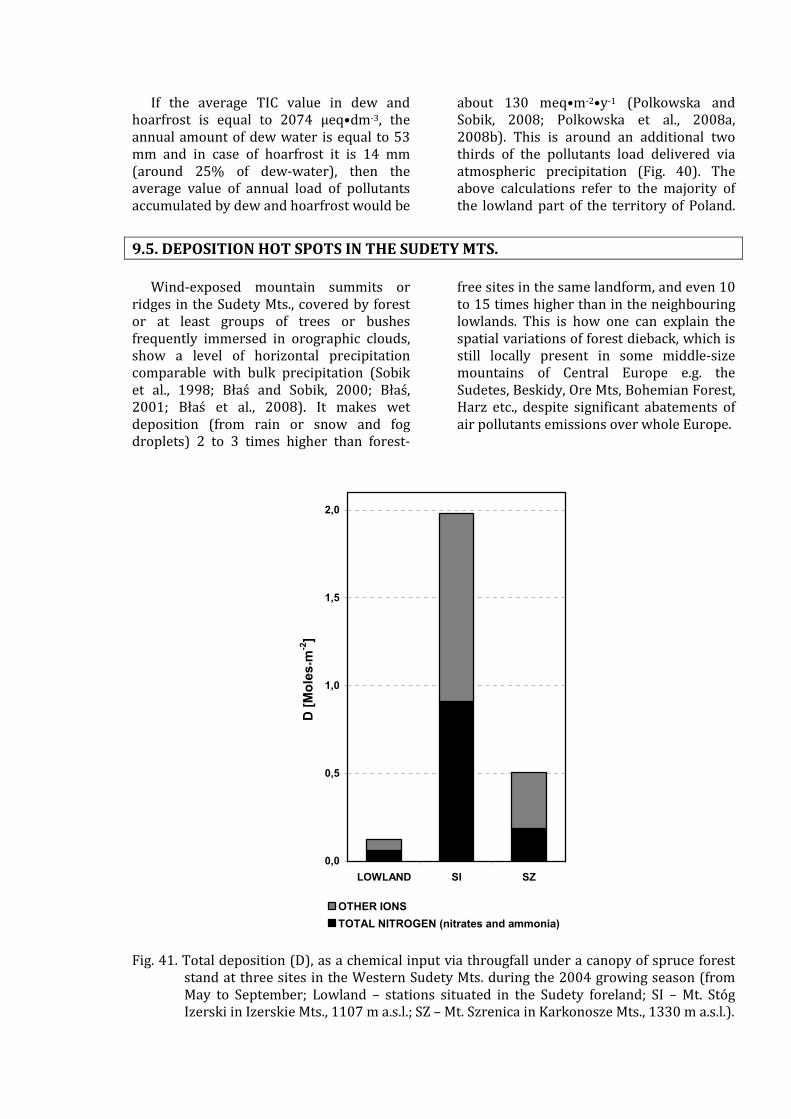
If the average TIC value in dew and hoarfrost is equal to 2074 µeq•dm-3, the annual amount of dew water is equal to 53 mm and in case of hoarfrost it is 14 mm (around 25% of dew-water), then the average value of annual load of pollutants accumulated by dew and hoarfrost would be

about 130 meq•m-2•y-1 (Polkowska and Sobik, 2008; Polkowska et al., 2008a, 2008b). This is around an additional two thirds of the pollutants load delivered via atmospheric precipitation (Fig. 40). The above calculations refer to the majority of the lowland part of the territory of Poland.

9.5. DEPOSITION HOT SPOTS IN THE SUDETY MTS.

Wind-exposed mountain summits or ridges in the Sudety Mts., covered by forest or at least groups of trees or bushes frequently immersed in orographic clouds, show a level of horizontal precipitation comparable with bulk precipitation (Sobik et al., 1998; Błaś and Sobik, 2000; Błaś, 2001; Błaś et al., 2008). It makes wet deposition (from rain or snow and fog droplets) 2 to 3 times higher than forest-

free sites in the same landform, and even 10 to 15 times higher than in the neighbouring lowlands. This is how one can explain the spatial variations of forest dieback, which is still locally present in some middle-size mountains of Central Europe e.g. the Sudetes, Beskidy, Ore Mts, Bohemian Forest, Harz etc., despite significant abatements of air pollutants emissions over whole Europe.

0,0

0,5

1,0

1,5

2,0

LOWLAND SI SZ

D [Moles*m

-2]

OTHER IONS

TOTAL NITROGEN (nitrates and ammonia)

Fig. 41. Total deposition (D), as a chemical input via througfall under a canopy of spruce forest stand at three sites in the Western Sudety Mts. during the 2004 growing season (from May to September; Lowland – stations situated in the Sudety foreland; SI – Mt. Stóg Izerski in Izerskie Mts., 1107 m a.s.l.; SZ – Mt. Szrenica in Karkonosze Mts., 1330 m a.s.l.).

Contribution of fog deposition to total deposition varies from a few percent over the lowland areas of Poland to up to 70 % in the mountainous regions (Fig. 41; Błaś and Sobik, 2003). Lowland fog is predominantly of radiation type, and usually develops under calm weather conditions. The main path of fog droplets deposition in this case is gravitational sedimentation of fog droplets, thus the efficiency of fog precipitation is very limited (Lovett, 1984). In the Sudety Mts., at elevations higher than 800 m a.s.l. fog/cloudwater deposition increases rapidly because of much higher wind speeds and turbulent flow of air (Błaś, 2001), which results in inertial impaction over sedimentation.

While Total Inorganic Ionic Content (TIC) values observed in lowland fog were 3-4 times higher in relation to Szrenica orographic fog, the total load of dissolved pollutants calculated per a volume unit of cloud was around 3-6 times higher at Szrenica Mt. (Błaś et al., 2010). Such differences are caused by 10-20 times higher liquid water content (LWC) of orographic fog, in contrary to lowland fog. According to the results of a recent experiment, the mean LWC in lowland was

measured as 0.015 g•m-3, whereas one can estimate LWC at Szrenica as 0.2-0.3 g•m-3 on average (Błaś, 1997).

Finally, the total deposition (the sum of major ions), measured as a chemical input by throughfall at the edge of the isolated forest stand during 5 months of the growing season of year 2004, equaled 1.98 Moles•m-

2 at the Stóg Izerski Mt. (1107 m a.s.l.) with nitrogen (from both nitrate and ammonia) being the main component (0.91 Moles•m-

2). This value is estimated to be the equivalent to 305.8 kg of N ha-1•yr-1, which can be compared to 20.2 kg of N ha-1•yr-1

under a spruce canopy at a nearby lowland site (Czerniawa-Zdrój; 480 m a.s.l.). Thus, the current nitrogen deposition at such hot spots situated in an igneous bedrock environment is around 20 times larger than the relevant critical value of nitrogen deposition (Błaś et al., 2008). At the same site (forest edge at the Stóg Izerski Mt.) around 30% of the total pollutant deposition came with precipitation and 70% with direct fog and cloud deposition, while the associated proportion at a nearby lowland site was around 95% and 5%, respectively.

9.6. REFERENCES Acker, K., Möller, D., Marquardt, W.,

Brüggemann, E., Wieprecht, W., Auel, R., Kalaβ, D., 1998, Atmospheric research program for studying changing emission patterns after German unifications. Atmospheric Environment 32, 3435-3443.

Beysens, D., 1995, The formation of dew. Atmospheric Research 39, 215-237.

Błaś, M., 1997. Experimental measurement of cloud liquid water content (LWC) in summer and winter conditions. Acta Universitatis Wratislaviensis., Prace Instytutu Geograficznego, Meteorologia i Klimatologia IV, 147-154.

Błaś, M., Sobik, M., 2000, Fog in the Giant Mountains and selected European massifs. Opera Corcontica, Proceeding of the International Conference “Geoecological Problems of the Giant Mountains”, Vrchlabi, 37, 35-46.

Błaś, M., 2001, Rola mgły w przychodzie wody i mokrej depozycji zanieczyszczeń w Sudetach. Maszynopis pracy doktorskiej, Wrocław,

Uniwersytet Wrocławski, Instytut Geograficzny, Zakład Meteorologii i Klimatologii.

Błaś, M., Sobik, M., Quiel, F., Netzel, P., 2002, Temporal and spatial variations of fog in the Western Sudety Mts., Poland. Atmospheric Research 64, 19-28.

Błaś, M., Sobik, M., 2003. Natural and human impact on pollutant deposition in mountain ecosystems with the Sudetes as an example. Studia Geograficzne 75, 420-438.

Błaś, M., Sobik M., Twarowski, R., 2008, Changes of cloudwater chemical composition in the Western Sudety Mountains, Poland. Atmospheric Research 87, 224-231.

Błaś M., Polkowska Ż., Sobik M., Klimaszewska K., Nowiński K., Namieśnik J., 2010, Fog water chemical composition in different geographic regions of Poland, Atmospheric Research 95, 455-469.

CIEP, 2006, Air Quality Monitoring of Chief Inspectorate of Environmental Protection, www.gios.gov.pl.

Collett Jr, J.L., Bator, A., Sherman, D.E., Moore, K.F., Hoag, K.J., Demoz, B.B., Rao, X., Reilly, J.E., 2002, The chemical composition of fogs and intercepted clouds in the United States. Atmospheric Research 64, 29-40.

Dore, A.J., Sobik, M., Migała, K., 1999. Patterns of precipitation and pollutant deposition in the Western Sudety Mountains, Poland. Atmospheric Environment 33, 3301-3312.

Ferrier, R.C., Jenkins, A., Elston, D.A., 1995. The composition of rime ice as an indicator of the quality of winter deposition. Environmental Pollution 87, 259-266.

Fišák, J., Řezáčová, D., 2001, Comparison between pollutant concentration in the samples of fog and rime water collected at Mt.Milesovka. Studia Geophysica et Geodaetica 45, 319-324.

Fišák, J., Tesař, M., Řezáčová, D., Elias, V., Weignerová, V., Fottová, D., 2004, Pollutant concentration in fog and low cloudwater at selected sites of the Czech Republic. Atmospheric Research 64, 75-87.

Hutorowicz, H., 1963, Dew measurements at Olsztyn. [In:] Assamblée Generale de Berkeley 1963, Gentbrugge1964 8', poz. bibl. UGGI Association International d’Hydrologie Scientifique 65, 352-359.

Lovett, G.M., 1984. Rates and mechanisms of cloudwater deposition to a subalpine balsam fir forest. Atmospheric Environment 18, 361-371.

Minami, Y., Ishizaka, Y., 1996, Evaluation of chemical composition in fog water near the summit of a high mountain in Japan. Atmospheric Environment 30, 3363-3376.

Muselli, M., Beysens, D., Marcillat, J., Milimouk, I., Nilsson, T., Louche, A., 2002, Dew water collector for potable water in Ajaccio, Atmospheric Research 64, 297- 312.

Polkowska, Ż., Sobik, M., 2008, Chemistry non-precipitation components of wet deposition with Poland as an example. [In:] Krope, J., Garbai, L., Kozic, D., Goricanec, G., Sakellaris, I.,

(eds.), Energy and Environmental III, Proceedings of the 3rd IASME/WSEAS International Conference on Energy & Environment (EE’08), University of Cambridge, UK, February 23-25, 349-354.

Polkowska, Ż., Błaś, M., Klimaszewska, K., Sobik, M., Małek, S., Namieśnik, J., 2008a, Chemical Characterization of Dew Water Collected in Different Geographic Regions of Poland. Sensors 8(6), 4006-4032.

Polkowska, Ż., Błaś, M., Sobik, M., Klimaszewska, K., Małek, S., Namiernik, J., 2008b, Wykorzystanie różnych form opadów i osadów atmosferycznych do oceny zanieczyszczenia środowiska w różnych regionach geograficznych Polski – część II – rosa. Ecological chemistry and engineering S, Vol. 15, No. 4, 530-559.

Puxbaum, H., Tscherwenka, W., 1998, Relationships of major ions in snow fall and rime at Sonnblick Observatory (SBO, 3106 m) and implications for scavenging processes in mixed clouds. Atmospheric Environment 32, 4011-4020.

Sobik, M., Błaś, M., Quiel, F., 1998, Udział osadów mgielnych w przychodzie wody z atmosfery i depozycji zanieczyszczeń w lasach Sudetów Zachodnich. [In:] “Geoekologiczne Problemy Karkonoszy" - Materiały z sesji naukowej w Przesiece 15-18.X.1997, Poznań, 151-162.

Sobik, M., 1999, Meteorologiczne uwarunkowania zakwaszenia hydrometeorów w Karkonoszach. Maszynopis pracy doktorskiej, Wrocław, Uniwersytet Wrocławski, Instytut Geograficzny, Zakład Meteorologii i Klimatologii.

Tesař, M., Fottová, D., Eliáš, V., Šír, M., 2000, Occult precipitation as an important contribution in Bohemian Forest. Silva Gabreta 4, 87-96.

Weathers, K.C., Simkin, S.M., Lovett, G.M., Lindberg, S.E., 2006, Empirical modelling of atmospheric deposition in mountainous landscapes. Empirical modelling of atmospheric deposition in mountainous landscapes. Ecological Applications 16, 1590-1607.