1

Liquefaction Analysis in Grenoble Basin by In Situ and Laboratory Tests

Draft of Master Dissertation Msc in Engineering Seismology ALPEREN SEYFI Supervisor: Prof. PIERRE FORAY

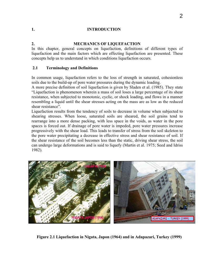
2 1. INTRODUCTION

2. MECHANICS OF LIQUEFACTION In this chapter, general concepts on liquefaction, definitions of different types of liquefaction and the main factors which are effecting liquefaction are presented. These concepts help us to understand in which conditions liquefaction occurs. 2.1 Terminology and Definitions In common usage, liquefaction refers to the loss of strength in saturated, cohesionless soils due to the build-up of pore water pressures during the dynamic loading. A more precise definition of soil liquefaction is given by Sladen et al. (1985). They state “Liquefaction is phenomenon wherein a mass of soil loses a large percentage of its shear resistance, when subjected to monotonic, cyclic, or shock loading, and flows in a manner resembling a liquid until the shear stresses acting on the mass are as low as the reduced shear resistance”. Liquefaction results from the tendency of soils to decrease in volume when subjected to shearing stresses. When loose, saturated soils are sheared, the soil grains tend to rearrange into a more dense packing, with less space in the voids, as water in the pore spaces is forced out. If drainage of pore water is impeded, pore water pressures increase progressively with the shear load. This leads to transfer of stress from the soil skeleton to the pore water precipitating a decrease in effective stress and shear resistance of soil. If the shear resistance of the soil becomes less than the static, driving shear stress, the soil can undergo large deformations and is said to liquefy (Martin et al. 1975; Seed and Idriss 1982).

Figure 2.1 Liquefaction in Nigata, Japon (1964) and in Adapazari, Turkey (1999)

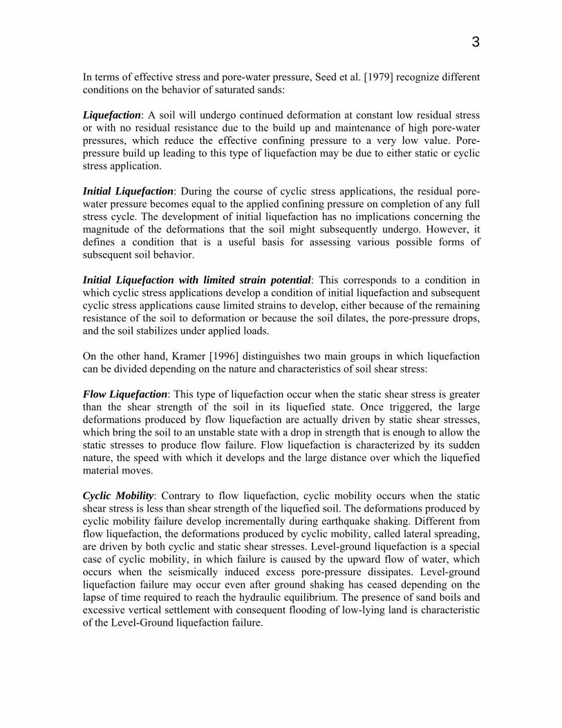
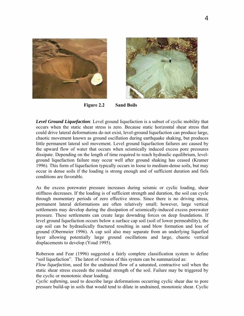
3 In terms of effective stress and pore-water pressure, Seed et al. [1979] recognize different conditions on the behavior of saturated sands: Liquefaction: A soil will undergo continued deformation at constant low residual stress or with no residual resistance due to the build up and maintenance of high pore-water pressures, which reduce the effective confining pressure to a very low value. Pore-pressure build up leading to this type of liquefaction may be due to either static or cyclic stress application. Initial Liquefaction: During the course of cyclic stress applications, the residual pore-water pressure becomes equal to the applied confining pressure on completion of any full stress cycle. The development of initial liquefaction has no implications concerning the magnitude of the deformations that the soil might subsequently undergo. However, it defines a condition that is a useful basis for assessing various possible forms of subsequent soil behavior. Initial Liquefaction with limited strain potential: This corresponds to a condition in which cyclic stress applications develop a condition of initial liquefaction and subsequent cyclic stress applications cause limited strains to develop, either because of the remaining resistance of the soil to deformation or because the soil dilates, the pore-pressure drops, and the soil stabilizes under applied loads. On the other hand, Kramer [1996] distinguishes two main groups in which liquefaction can be divided depending on the nature and characteristics of soil shear stress: Flow Liquefaction: This type of liquefaction occur when the static shear stress is greater than the shear strength of the soil in its liquefied state. Once triggered, the large deformations produced by flow liquefaction are actually driven by static shear stresses, which bring the soil to an unstable state with a drop in strength that is enough to allow the static stresses to produce flow failure. Flow liquefaction is characterized by its sudden nature, the speed with which it develops and the large distance over which the liquefied material moves. Cyclic Mobility: Contrary to flow liquefaction, cyclic mobility occurs when the static shear stress is less than shear strength of the liquefied soil. The deformations produced by cyclic mobility failure develop incrementally during earthquake shaking. Different from flow liquefaction, the deformations produced by cyclic mobility, called lateral spreading, are driven by both cyclic and static shear stresses. Level-ground liquefaction is a special case of cyclic mobility, in which failure is caused by the upward flow of water, which occurs when the seismically induced excess pore-pressure dissipates. Level-ground liquefaction failure may occur even after ground shaking has ceased depending on the lapse of time required to reach the hydraulic equilibrium. The presence of sand boils and excessive vertical settlement with consequent flooding of low-lying land is characteristic of the Level-Ground liquefaction failure.

4

Figure 2.2 Sand Boils Level Ground Liquefaction: Level ground liquefaction is a subset of cyclic mobility that occurs when the static shear stress is zero. Because static horizontal shear stress that could drive lateral deformations do not exist, level-ground liquefaction can produce large, chaotic movement known as ground oscillation during earthquake shaking, but produces little permanent lateral soil movement. Level ground liquefaction failures are caused by the upward flow of water that occurs when seismically induced excess pore pressures dissipate. Depending on the length of time required to reach hydraulic equilibrium, level-ground liquefaction failure may occur well after ground shaking has ceased (Kramer 1996). This form of liquefaction typically occurs in loose to medium-dense soils, but may occur in dense soils if the loading is strong enough and of sufficient duration and fiels conditions are favorable. As the excess porewater pressure increases during seismic or cyclic loading, shear stiffness decreases. If the loading is of sufficient strength and duration, the soil can cycle through momentary periods of zero effective stress. Since there is no driving stress, permanent lateral deformations are often relatively small; however, large vertical settlements may develop during the dissipation of seismically-induced excess porewater pressure. These settlements can create large downdrag forces on deep foundations. If level ground liquefaction occurs below a surface cap soil (soil of lower permeability), the cap soil can be hydraulically fractured resulting in sand blow formation and loss of ground (Obermeier 1996). A cap soil also may separate from an underlying liquefied layer allowing potentially large ground oscillations and large, chaotic vertical displacements to develop (Youd 1995). Roberson and Fear (1996) suggested a fairly complete classification system to define “soil liquefaction”. The latest of version of this system can be summarized as: Flow liquefaction, used for the undrained flow of a saturated, contractive soil when the static shear stress exceeds the residual strength of the soil. Failure may be triggered by the cyclic or monotonic shear loading. Cyclic softening, used to describe large deformations occurring cyclic shear due to pore pressure build-up in soils that would tend to dilate in undrained, monotonic shear. Cyclic

5softening, in which deformations do not continue after cyclic loading ceases, can be further classified as;

• Cyclic liquefaction, which occurs when cyclic shear stresses exceed the initial, static shear stress to produce a stress reversal. A condition of zero effective stress may be achieved during which larger deformations may occur.

• Cyclic mobility, in which cyclic loads do not yield a shear stress reversal and a condition of zero effective stress does not develop. Deformations accumulate in each cycle of shear stress.

During cyclic undrained loading almost all saturated cohesionless soil develop positive pore water pressures due to the contractive response of the soil at small strains. If there is shear stress reversal, the effective stress state can progress to the point of essentially zero effective stress, as illustrated in the figure 1. When the soil element reaches the condition of essentially zero effective stress, the soil has very little stiffness and large deformations can occur during cyclic loading. If there is no shear stress reversal, the stress state may not reach zero effective stress. (Robertson and Wride 1996) 2.2 Liquefaction Susceptibility Liquefaction is most commonly observed in shallow, loose, saturated deposits of cohesionless soils subjected to strong ground motions in large-magnitude earthquakes. Unsaturated soils are not subjected to liquefaction because volume compression does not generate excess pore pressures. Liquefaction and large deformations are more likely with contractive soils while cyclic softening and limited deformations are associated with dilative soils. Other factors affecting liquefaction susceptibility of different soil types are discussed in this section. 2.2.1 Factors Affecting Liquefaction 2.2.1.1 Moment Magnitude and Epicentral Distance Based on historical registers, Ambraseys [1988] compiled worldwide data from shallow earthquakes in order to estimate a limiting epicentral distance beyond which liquefaction has not been observed in earthquakes of different magnitudes. Figure 2.3 shows that distance to which liquefaction can be expected increases dramatically with increasing magnitude. Ambraseys reported that deep earthquakes with focal depth greater than 50 km have produced liquefaction at greater distances.

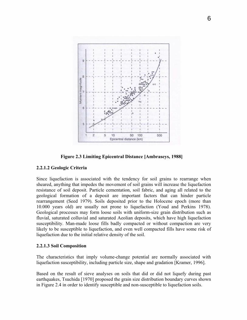
6 Figure 2.3 Limiting Epicentral Distance [Ambraseys, 1988] 2.2.1.2 Geologic Criteria Since liquefaction is associated with the tendency for soil grains to rearrange when sheared, anything that impedes the movement of soil grains will increase the liquefaction resistance of soil deposit. Particle cementation, soil fabric, and aging all related to the geological formation of a deposit are important factors that can hinder particle rearrangement (Seed 1979). Soils deposited prior to the Holocene epoch (more than 10.000 years old) are usually not prone to liquefaction (Youd and Perkins 1978). Geological processes may form loose soils with uniform-size grain distribution such as fluvial, saturated colluvial and saturated Aeolian deposits, which have high liquefaction susceptibility. Man-made loose fills badly compacted or without compaction are very likely to be susceptible to liquefaction, and even well compacted fills have some risk of liquefaction due to the initial relative density of the soil. 2.2.1.3 Soil Composition The characteristics that imply volume-change potential are normally associated with liquefaction susceptibility, including particle size, shape and gradation [Kramer, 1996]. Based on the result of sieve analyses on soils that did or did not liquefy during past earthquakes, Tsuchida [1970] proposed the grain size distribution boundary curves shown in Figure 2.4 in order to identify susceptible and non-susceptible to liquefaction soils.

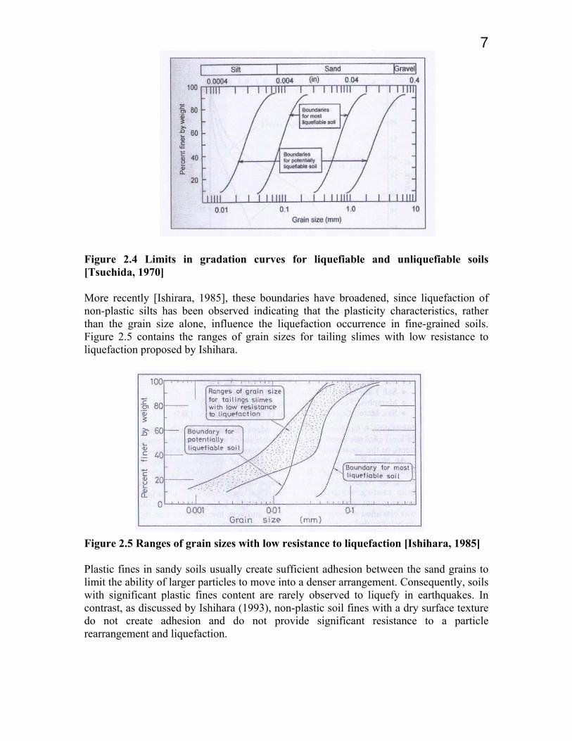
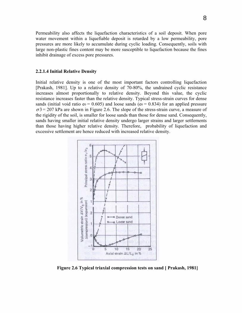
7 Figure 2.4 Limits in gradation curves for liquefiable and unliquefiable soils [Tsuchida, 1970] More recently [Ishirara, 1985], these boundaries have broadened, since liquefaction of non-plastic silts has been observed indicating that the plasticity characteristics, rather than the grain size alone, influence the liquefaction occurrence in fine-grained soils. Figure 2.5 contains the ranges of grain sizes for tailing slimes with low resistance to liquefaction proposed by Ishihara. Figure 2.5 Ranges of grain sizes with low resistance to liquefaction [Ishihara, 1985] Plastic fines in sandy soils usually create sufficient adhesion between the sand grains to limit the ability of larger particles to move into a denser arrangement. Consequently, soils with significant plastic fines content are rarely observed to liquefy in earthquakes. In contrast, as discussed by Ishihara (1993), non-plastic soil fines with a dry surface texture do not create adhesion and do not provide significant resistance to a particle rearrangement and liquefaction.

8 Permeability also affects the liquefaction characteristics of a soil deposit. When pore water movement within a liquefiable deposit is retarded by a low permeability, pore pressures are more likely to accumulate during cyclic loading. Consequently, soils with large non-plastic fines content may be more susceptible to liquefaction because the fines inhibit drainage of excess pore pressures. 2.2.1.4 Initial Relative Density Initial relative density is one of the most important factors controlling liquefaction [Prakash, 1981]. Up to a relative density of 70-80%, the undrained cyclic resistance increases almost proportionally to relative density. Beyond this value, the cyclic resistance increases faster than the relative density. Typical stress-strain curves for dense sands (initial void ratio e0 = 0.605) and loose sands (e0 = 0.834) for an applied pressure

3σ = 207 kPa are shown in Figure 2.6. The slope of the stress-strain curve, a measure of the rigidity of the soil, is smaller for loose sands than those for dense sand. Consequently, sands having smaller initial relative density undergo larger strains and larger settlements than those having higher relative density. Therefore, probability of liquefaction and excessive settlement are hence reduced with increased relative density. Figure 2.6 Typical triaxial compression tests on sand [ Prakash, 1981]

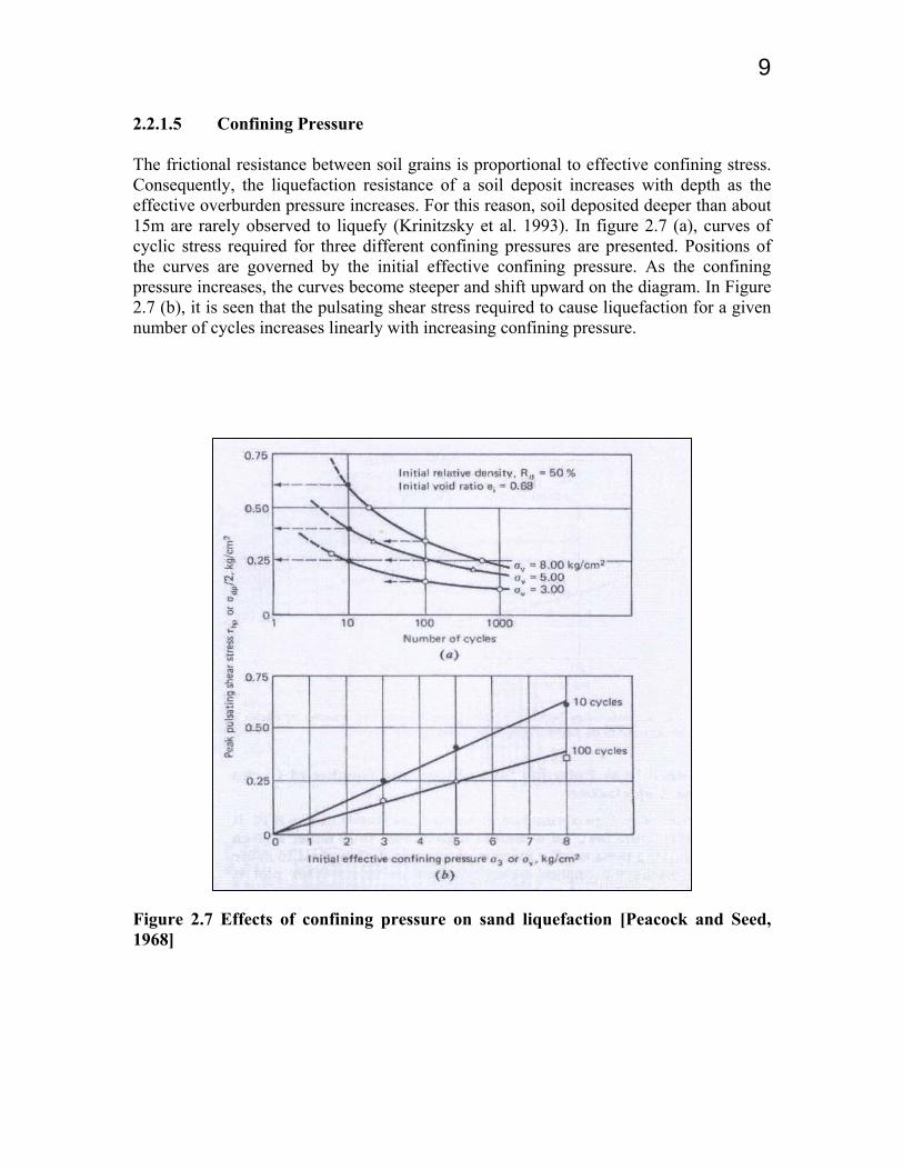
9 2.2.1.5 Confining Pressure The frictional resistance between soil grains is proportional to effective confining stress. Consequently, the liquefaction resistance of a soil deposit increases with depth as the effective overburden pressure increases. For this reason, soil deposited deeper than about 15m are rarely observed to liquefy (Krinitzsky et al. 1993). In figure 2.7 (a), curves of cyclic stress required for three different confining pressures are presented. Positions of the curves are governed by the initial effective confining pressure. As the confining pressure increases, the curves become steeper and shift upward on the diagram. In Figure 2.7 (b), it is seen that the pulsating shear stress required to cause liquefaction for a given number of cycles increases linearly with increasing confining pressure. Figure 2.7 Effects of confining pressure on sand liquefaction [Peacock and Seed, 1968]

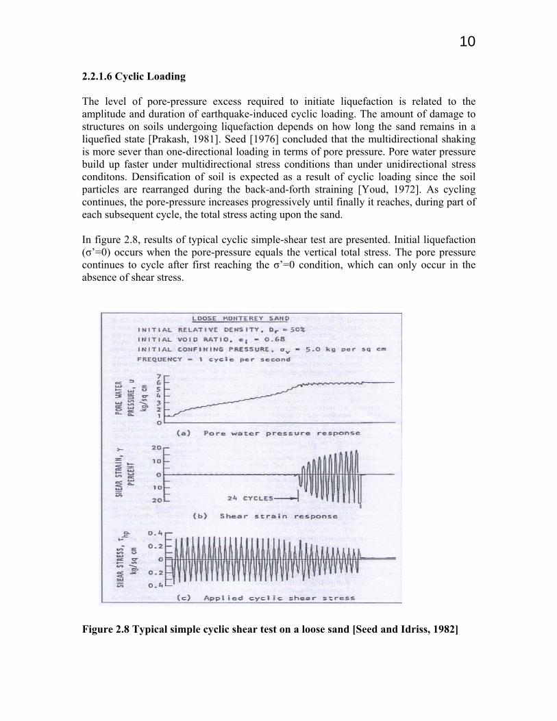
10 2.2.1.6 Cyclic Loading The level of pore-pressure excess required to initiate liquefaction is related to the amplitude and duration of earthquake-induced cyclic loading. The amount of damage to structures on soils undergoing liquefaction depends on how long the sand remains in a liquefied state [Prakash, 1981]. Seed [1976] concluded that the multidirectional shaking is more sever than one-directional loading in terms of pore pressure. Pore water pressure build up faster under multidirectional stress conditions than under unidirectional stress conditons. Densification of soil is expected as a result of cyclic loading since the soil particles are rearranged during the back-and-forth straining [Youd, 1972]. As cycling continues, the pore-pressure increases progressively until finally it reaches, during part of each subsequent cycle, the total stress acting upon the sand. In figure 2.8, results of typical cyclic simple-shear test are presented. Initial liquefaction (σ’=0) occurs when the pore-pressure equals the vertical total stress. The pore pressure continues to cycle after first reaching the σ’=0 condition, which can only occur in the absence of shear stress.

Figure 2.8 Typical simple cyclic shear test on a loose sand [Seed and Idriss, 1982]

11 2.3 Ground Failures Resulting from Soil Liquefaction Eight types of failure commonly associated with soil liquefaction in earthquakes:

• Sand boils, which usually result in subsidence and relatively minor damage. • Flow failures of slopes involving very large down-slope movements of a soil

mass. • Lateral spreads resulting from the lateral displacement of gently sloping ground. • Ground oscillation where liquefaction of a soil deposit beneath a level site leads

to back and forth movements of intact blocks of surface soil. • Loss of bearing capacity causing foundations failures. • Buoyant rise of buried structures such as tanks. • Ground settlement, often associated with some other failure mechanism. • Failure of retaining walls due to increased lateral loads from liquefied backfill

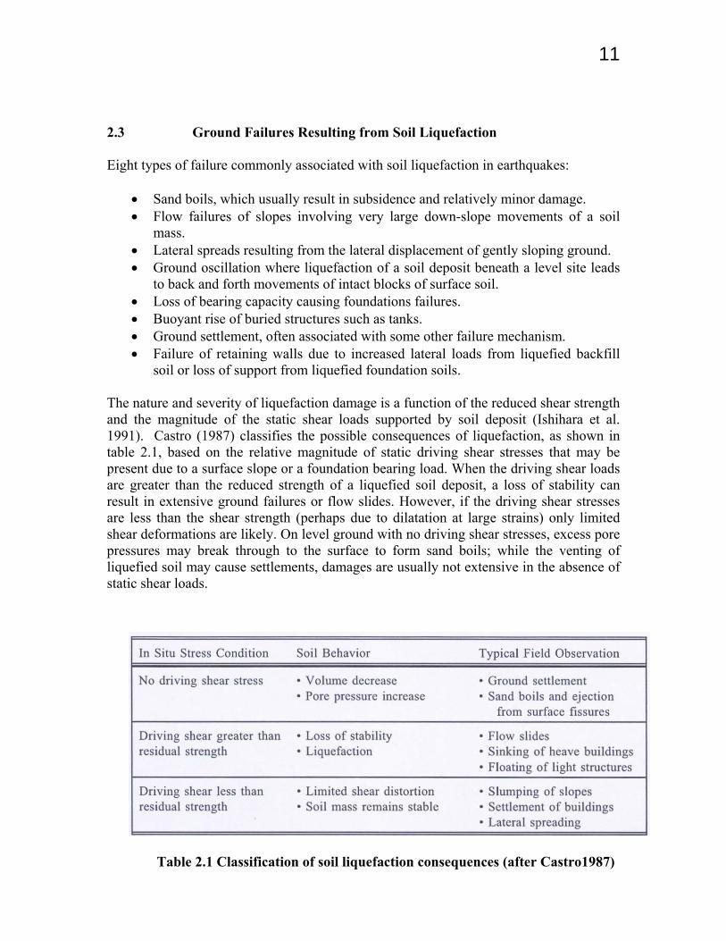
soil or loss of support from liquefied foundation soils. The nature and severity of liquefaction damage is a function of the reduced shear strength and the magnitude of the static shear loads supported by soil deposit (Ishihara et al. 1991). Castro (1987) classifies the possible consequences of liquefaction, as shown in table 2.1, based on the relative magnitude of static driving shear stresses that may be present due to a surface slope or a foundation bearing load. When the driving shear loads are greater than the reduced strength of a liquefied soil deposit, a loss of stability can result in extensive ground failures or flow slides. However, if the driving shear stresses are less than the shear strength (perhaps due to dilatation at large strains) only limited shear deformations are likely. On level ground with no driving shear stresses, excess pore pressures may break through to the surface to form sand boils; while the venting of liquefied soil may cause settlements, damages are usually not extensive in the absence of static shear loads.

Table 2.1 Classification of soil liquefaction consequences (after Castro1987)

12 Ground failures associated with liquefaction under cyclic loading can be classified as (Robertson et al. 1992):

(1) Flow failures, occurring when the liquefaction of loose, contractive soils (that do not gain strength at large shear strains) results in very large deformations.

(2) Deformation failures, occurring when a liquefied soils gains shear resistance at large strains, yielding limited deformations without loss of stability.

2.4 Behavior of Saturated, Cohesionless Soils in Undrained Shear During an earthquake, the upward propagation of shear waves through the ground generates shear stresses and strains that are cyclic in nature (Seed and Idriss 1982). If a cohesionless soil is saturated, excess pore pressures may accumulate during seismic shearing and lead to liquefaction. A loose soil tends to compact when sheared and, without drainage, pore water pressures increase. As indicated in Figure2.9a, a contractive soil sheared monotonically reaches a peak shear strength and then softens, eventually achieving a residual shear resistance. If the residual shear strength is less than the static driving shear, liquefaction flow failure results. If the same soil is sheared cyclicly, excess pore pressures are generated with each cycle of load. Without drainage, pore pressures accumulate and the effective stress path moves toward failure. If the shear strength falls below the static driving stress, a flow failure results and deformations continue after cyclic loading stops. For a liquefaction flow failure to occur, a saturated soil with a tendency to contract must undergo undrained shear of sufficient magnitude, or sufficient number of load cycles, for the shear resistance to become less than the static driving load. Under these conditions, tremendous deformations may occur before equilibrium conditions are re-established at the reduced shear strength. Shearing of dense, dilative soils will also produce some excess pore pressure at small strains. However, at larger strains, the pore pressures decrease and can become negative as the soil grains, moving up and over one another, tend to cause an increase in soil volume (dilation). Consequently, as shown in Figure 2.9b, monotonic shearing of a dilative soil results in an increasing effective stress and shear resistance. Figure 2.9b also shows the response of the same dilative soil to dynamic loading. In this case, pore pressures are generated in each shear cycle resulting in an accumulation of excess pore pressure and deformation. However, beyond some point the tendency to dilate and develop negative pore pressures limits further straining in additional load cycles. As indicated in the bottom of figure 2.9b, the effective stress path moves to the left but never reaches the failure surface. If the soil is sheared after the cyclic load ceases, the soil will develop the full strength that would be observed in a monotonic shear test. While significant strains can occur during cyclic loading, the very large deformations associated with a flow failure do not develop in dense, dilative soils. Hence, cyclic shear of dilative soils does not result in flow failures because, with undrained conditions, the shear strength remains greater than the static driving shear stress.

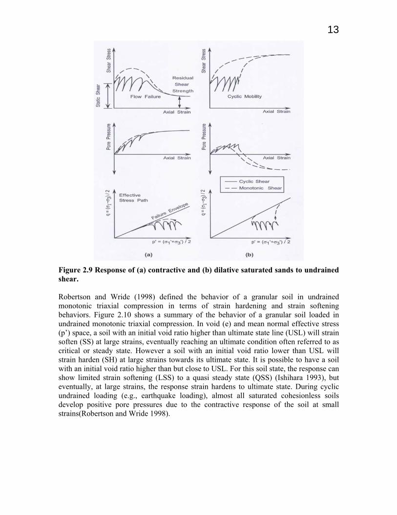
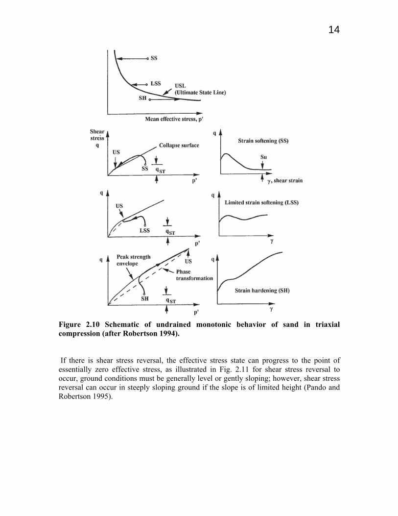
13 Figure 2.9 Response of (a) contractive and (b) dilative saturated sands to undrained shear. Robertson and Wride (1998) defined the behavior of a granular soil in undrained monotonic triaxial compression in terms of strain hardening and strain softening behaviors. Figure 2.10 shows a summary of the behavior of a granular soil loaded in undrained monotonic triaxial compression. In void (e) and mean normal effective stress (p’) space, a soil with an initial void ratio higher than ultimate state line (USL) will strain soften (SS) at large strains, eventually reaching an ultimate condition often referred to as critical or steady state. However a soil with an initial void ratio lower than USL will strain harden (SH) at large strains towards its ultimate state. It is possible to have a soil with an initial void ratio higher than but close to USL. For this soil state, the response can show limited strain softening (LSS) to a quasi steady state (QSS) (Ishihara 1993), but eventually, at large strains, the response strain hardens to ultimate state. During cyclic undrained loading (e.g., earthquake loading), almost all saturated cohesionless soils develop positive pore pressures due to the contractive response of the soil at small strains(Robertson and Wride 1998).

14

Figure 2.10 Schematic of undrained monotonic behavior of sand in triaxial compression (after Robertson 1994). If there is shear stress reversal, the effective stress state can progress to the point of essentially zero effective stress, as illustrated in Fig. 2.11 for shear stress reversal to occur, ground conditions must be generally level or gently sloping; however, shear stress reversal can occur in steeply sloping ground if the slope is of limited height (Pando and Robertson 1995).

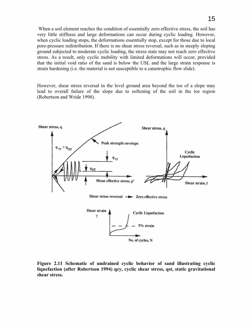
15 When a soil element reaches the condition of essentially zero effective stress, the soil has very little stiffness and large deformations can occur during cyclic loading. However, when cyclic loading stops, the deformations essentially stop, except for those due to local pore-pressure redistribution. If there is no shear stress reversal, such as in steeply sloping ground subjected to moderate cyclic loading, the stress state may not reach zero effective stress. As a result, only cyclic mobility with limited deformations will occur, provided that the initial void ratio of the sand is below the USL and the large strain response is strain hardening (i.e. the material is not susceptible to a catastrophic flow slide). However, shear stress reversal in the level ground area beyond the toe of a slope may lead to overall failure of the slope due to softening of the soil in the toe region (Robertson and Wride 1998).

Figure 2.11 Schematic of undrained cyclic behavior of sand illustrating cyclic liquefaction (after Robertson 1994) qcy, cyclic shear stress, qst, static gravitational shear stress.

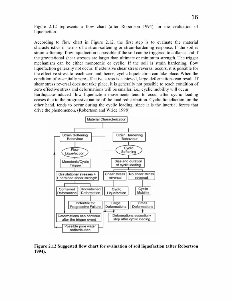
16Figure 2.12 represents a flow chart (after Robertson 1994) for the evaluation of liquefaction. According to flow chart in Figure 2.12, the first step is to evaluate the material characteristics in terms of a strain-softening or strain-hardening response. If the soil is strain softening, flow liquefaction is possible if the soil can be triggered to collapse and if the gravitational shear stresses are larger than ultimate or minimum strength. The trigger mechanism can be either monotonic or cyclic. If the soil is strain hardening, flow liquefaction generally not occur. If extensive shear stress reversal occurs, it is possible for the effective stress to reach zero and, hence, cyclic liquefaction can take place. When the condition of essentially zero effective stress is achieved, large deformations can result. If shear stress reversal does not take place, it is generally not possible to reach condition of zero effective stress and deformations will be smaller, i.e., cyclic mobility will occur. Earthquake-induced flow liquefaction movements tend to occur after cyclic loading ceases due to the progressive nature of the load redistribution. Cyclic liquefaction, on the other hand, tends to occur during the cyclic loading, since it is the intertial forces that drive the phenomenon. (Robertson and Wride 1998) Figure 2.12 Suggested flow chart for evaluation of soil liquefaction (after Robertson 1994).

17CHAPTER 3

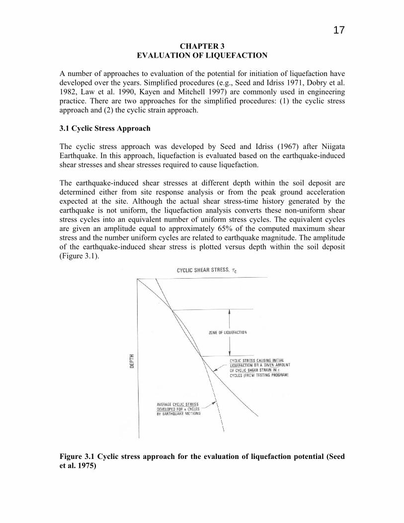
EVALUATION OF LIQUEFACTION A number of approaches to evaluation of the potential for initiation of liquefaction have developed over the years. Simplified procedures (e.g., Seed and Idriss 1971, Dobry et al. 1982, Law et al. 1990, Kayen and Mitchell 1997) are commonly used in engineering practice. There are two approaches for the simplified procedures: (1) the cyclic stress approach and (2) the cyclic strain approach. 3.1 Cyclic Stress Approach The cyclic stress approach was developed by Seed and Idriss (1967) after Niigata Earthquake. In this approach, liquefaction is evaluated based on the earthquake-induced shear stresses and shear stresses required to cause liquefaction. The earthquake-induced shear stresses at different depth within the soil deposit are determined either from site response analysis or from the peak ground acceleration expected at the site. Although the actual shear stress-time history generated by the earthquake is not uniform, the liquefaction analysis converts these non-uniform shear stress cycles into an equivalent number of uniform stress cycles. The equivalent cycles are given an amplitude equal to approximately 65% of the computed maximum shear stress and the number uniform cycles are related to earthquake magnitude. The amplitude of the earthquake-induced shear stress is plotted versus depth within the soil deposit (Figure 3.1). Figure 3.1 Cyclic stress approach for the evaluation of liquefaction potential (Seed et al. 1975)

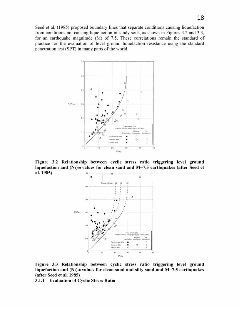
18Seed et al. (1985) proposed boundary lines that separate conditions causing liquefaction from conditions not causing liquefaction in sandy soils, as shown in Figures 3.2 and 3.3, for an earthquake magnitude (M) of 7.5. These correlations remain the standard of practice for the evaluation of level ground liquefaction resistance using the standard penetration test (SPT) in many parts of the world. Figure 3.2 Relationship between cyclic stress ratio triggering level ground liquefaction and (N1)60 values for clean sand and M=7.5 earthquakes (after Seed et al. 1985) Figure 3.3 Relationship between cyclic stress ratio triggering level ground liquefaction and (N1)60 values for clean sand and silty sand and M=7.5 earthquakes (after Seed et al. 1985) 3.1.1 Evaluation of Cyclic Stress Ratio

19Seed et al. (1985) used equivalent cyclic stress ratio CSReq, to represent the intensity of earthquake loading. Since CSReq pertains to a certain number of equivalent laboratory loading cycles corresponding to a given earthquake magnitude, Stark and Mesri (1992) proposed the term seismic (shear) stress ratio, SSR, to describe earthquake loading. They suggested that SSR is more descriptive of field earthquake loading than equivalent cyclic stress ratio. Seed and Idriss (1971) proposed the “simplified” equation to estimate the equivalent cyclic shear stress ratio (or seismic shear stress ratio) induced by an earthquake. The resulting seismic (shear) stress ratio is defined as:

rdvovo

ga

vovoaveqCSSSR

'max65.0

'max65.0

'Re

σσ

στ

στ

≈≈== (3.1)

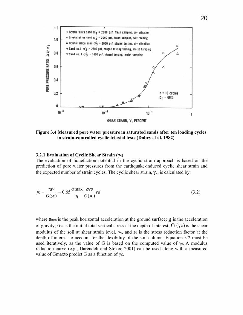
where the τave is the average earthquake-induced shear stress, τmax is the maximum earthquake-induced shear stress, σ’vo is the vertical effective stress, amax is the maximum earthquake acceleration at the ground surface, g is the acceleration of gravity, σvo is the vertical total stress, and rd is a depth reduction factor to account for the flexibility of the soil column. 3.2 Cyclic Strain Approach The cyclic strain approach for evaluating the liquefaction potential was first introduced by Dobry et al. (1982). In this approach, shear strain, rather than shear stress, is the main parameter that controls both densification and liquefaction in sands. Dobry et al. (1982) found a strong relationship between cyclic shear strain and pore water pressure generation, as presented in Figure 3.4. The data shown in Figure 3.4 were obtained from cyclic strain-controlled triaxial tests performed on two types of clean sands. The pore water pressure response of both sands after ten loading cycles revealed the existence of a cyclic threshold shear strain of approximately 0.01%, below which no densification of the soil (if allowed to drain) or pore water pressure generation occurs. The trend of these data also showed that approximately 10 cycles of 1% cyclic shear strain would generate a pore water pressure ratio of 1.0, which corresponds to zero effective stress and thus initial liquefaction of the specimen.

20

Figure 3.4 Measured pore water pressure in saturated sands after ten loading cycles in strain-controlled cyclic triaxial tests (Dobry et al. 1982) 3.2.1 Evaluation of Cyclic Shear Strain (γc) The evaluation of liquefaction potential in the cyclic strain approach is based on the prediction of pore water pressures from the earthquake-induced cyclic shear strain and the expected number of strain cycles. The cyclic shear strain, γc, is calculated by:

rdcG

vog

acG

avc)(

max65.0)( γ

σγ

τγ == (3.2)

where amax is the peak horizontal acceleration at the ground surface; g is the acceleration of gravity; σvo is the initial total vertical stress at the depth of interest; G (γc) is the shear modulus of the soil at shear strain level, γc, and rd is the stress reduction factor at the depth of interest to account for the flexibility of the soil column. Equation 3.2 must be used iteratively, as the value of G is based on the computed value of γc. A modulus reduction curve (e.g., Darendeli and Stokoe 2001) can be used along with a measured value of Gmaxto predict G as a function of γc.

21 3.3 Characterization of Liquefaction Resistance The liquefaction resistance of an element of soil depends on how close the initial state of the soil is to the state corresponding to “failure” and on the nature of the loading required to move it from the initial state to the failure state (Kramer, 1996). Two basic approaches have been used to predict the liquefaction potential of soil strata (De Alba et al. 1976; Seed 1979; Seed et al. 1983):

(1) Evaluations based on a comparison of the stresses induced by an earthquake and the stress conditions causing liquefaction in cyclic laboratory tests on soil samples.

(2) Empirical methods based on measurements of in situ soil strength and observations of field performance in previous earthquakes.

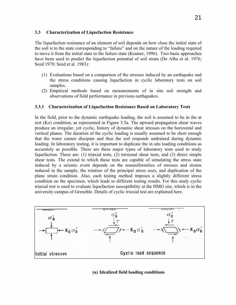
3.3.1 Characterization of Liquefaction Resistance Based on Laboratory Tests In the field, prior to the dynamic earthquake loading, the soil is assumed to be in the at rest (Ko) condition, as represented in Figure 3.5a. The upward propagation shear waves produce an irregular, yet cyclic, history of dynamic shear stresses on the horizontal and vertical planes. The duration of the cyclic loading is usually assumed to be short enough that the water cannot dissipate and thus the soil responds undrained during dynamic loading. In laboratory testing, it is important to duplicate the in situ loading conditions as accurately as possible. There are three major types of laboratory tests used to study liquefaction. These are: (1) triaxial tests, (2) torsional shear tests, and (3) direct simple shear tests. The extend to which these tests are capable of simulating the stress state induced by a seismic event depends on the nonuniformities of stresses and strains induced in the sample, the rotation of the principal stress axes, and duplication of the plane strain condition. Also, each testing method imposes a slightly different stress condition on the specimen, which leads to different testing results. For this study cyclic triaxial test is used to evaluate liquefaction susceptibility at the HMG site, which is in the university campus of Grenoble. Details of cyclic triaxial test are explained here.

(a) Idealized field loading conditions

22

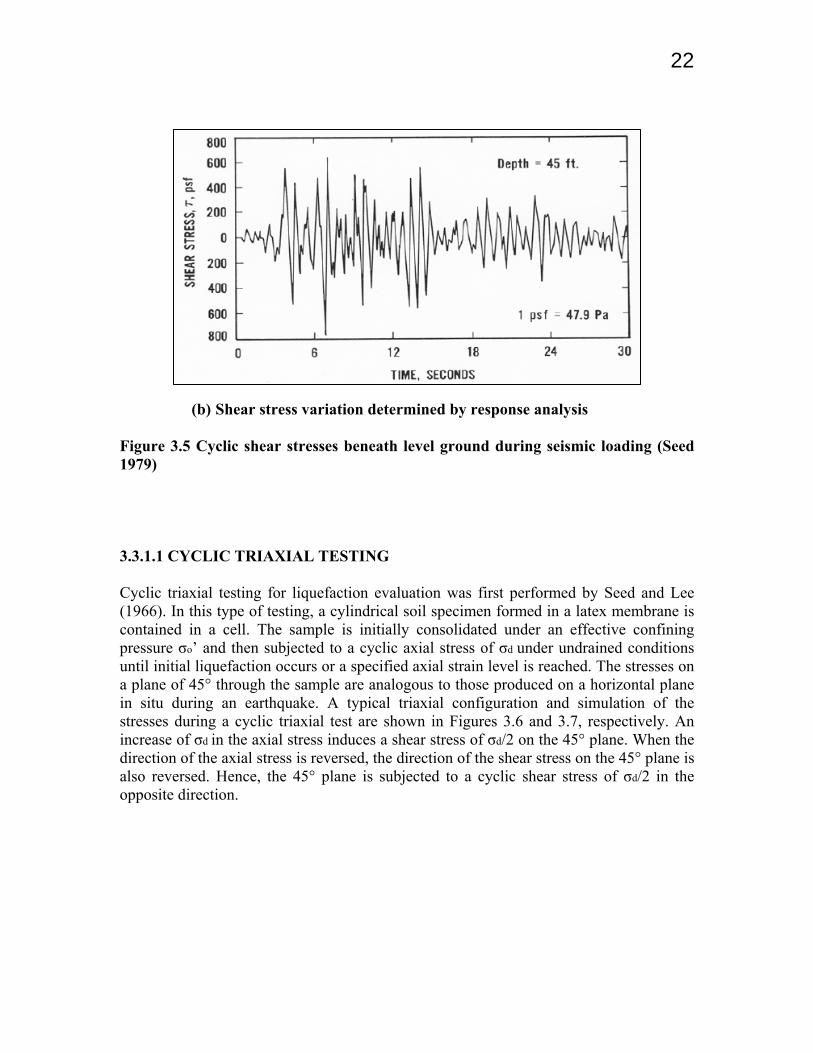
(b) Shear stress variation determined by response analysis Figure 3.5 Cyclic shear stresses beneath level ground during seismic loading (Seed 1979) 3.3.1.1 CYCLIC TRIAXIAL TESTING Cyclic triaxial testing for liquefaction evaluation was first performed by Seed and Lee (1966). In this type of testing, a cylindrical soil specimen formed in a latex membrane is contained in a cell. The sample is initially consolidated under an effective confining pressure σo’ and then subjected to a cyclic axial stress of σd under undrained conditions until initial liquefaction occurs or a specified axial strain level is reached. The stresses on a plane of 45° through the sample are analogous to those produced on a horizontal plane in situ during an earthquake. A typical triaxial configuration and simulation of the stresses during a cyclic triaxial test are shown in Figures 3.6 and 3.7, respectively. An increase of σd in the axial stress induces a shear stress of σd/2 on the 45° plane. When the direction of the axial stress is reversed, the direction of the shear stress on the 45° plane is also reversed. Hence, the 45° plane is subjected to a cyclic shear stress of σd/2 in the opposite direction.

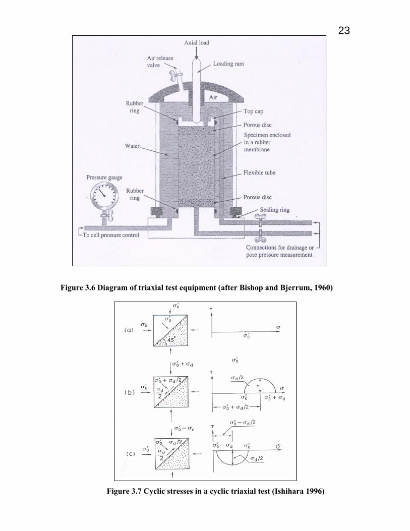
23

Figure 3.6 Diagram of triaxial test equipment (after Bishop and Bjerrum, 1960) Figure 3.7 Cyclic stresses in a cyclic triaxial test (Ishihara 1996)

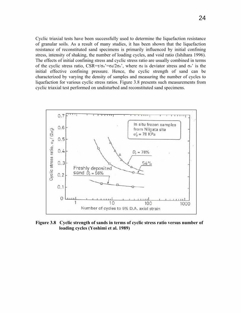
24 Cyclic triaxial tests have been successfully used to determine the liquefaction resistance of granular soils. As a result of many studies, it has been shown that the liquefaction resistance of reconstituted sand specimens is primarily influenced by initial confining stress, intensity of shaking, the number of loading cycles, and void ratio (Ishihara 1996). The effects of initial confining stress and cyclic stress ratio are usually combined in terms of the cyclic stress ratio, CSR=τ/σo’=σd/2σo’, where σd is deviator stress and σo’ is the initial effective confining pressure. Hence, the cyclic strength of sand can be characterized by varying the density of samples and measuring the number of cycles to liquefaction for various cyclic stress ratios. Figure 3.8 presents such measurements from cyclic triaxial test performed on undisturbed and reconstituted sand specimens.

Figure 3.8 Cyclic strength of sands in terms of cyclic stress ratio versus number of loading cycles (Yoshimi et al. 1989)

253.3.2 Characterization of Liquefaction Resistance Based on In Situ Tests To evaluate the liquefaction resistance (shear stress required to cause liquefaction in a number of loading cycles), cyclic laboratory testing on representative samples can be performed or the liquefaction resistance can be correlated with in situ tests such as the Standard Penetration Test (SPT). When performing laboratory tests, the tests provide data regarding the shear stress level that causes liquefaction in the number of expected earthquake loading cycles. This is sometimes called cyclic strength. When using in situ correlations, the shear stress level required to cause liquefaction in a given number of cycles is empirically related to in situ test parameters such as SPT blow count (N1,60; Seed et al. 1985), the Cone Penetration Test (CPT) tip resistance (qc1n; Robertson and Wride 1998) or soil shear wave velocity (Vs1; Andrus and Stokoe 2000). Unfortunately, liquefaction assessments based on laboratory tests are hindered by limitations in the ability of laboratory equipment to reproduce field stress conditions in small soil samples. Even more problematic, disturbance of filed samples is nearly impossible to avoid and very difficult to quantify in laboratory tests (Seed 1979). As a result, early evaluations based on laboratory tests were often overly conservative in predicting liquefaction (Peck 1979). Because the empirical correlations are simple and incorporate a limited number of parameters, the simplified procedure is widely used in practice. 3.3.2.1 Method Based on the Standard Penetration Test Seed et al. (1985) investigated sites that did and did not experience liquefaction during earthquakes. The empirical chart published by Seed et al. (1985) is based on a standardized SPT blowcount, (N1)60, and the cyclic stress ratio (CSR). To get (N1)60, the measured NSPT is corrected for the energy delivered by different hammer systems and normalized with respect to overburden stress. Seed et al. found that for the same stress-corrected penetration resistance, (N1)60, the liquefaction resistance increases with increasing fine content (Figure 3.9).

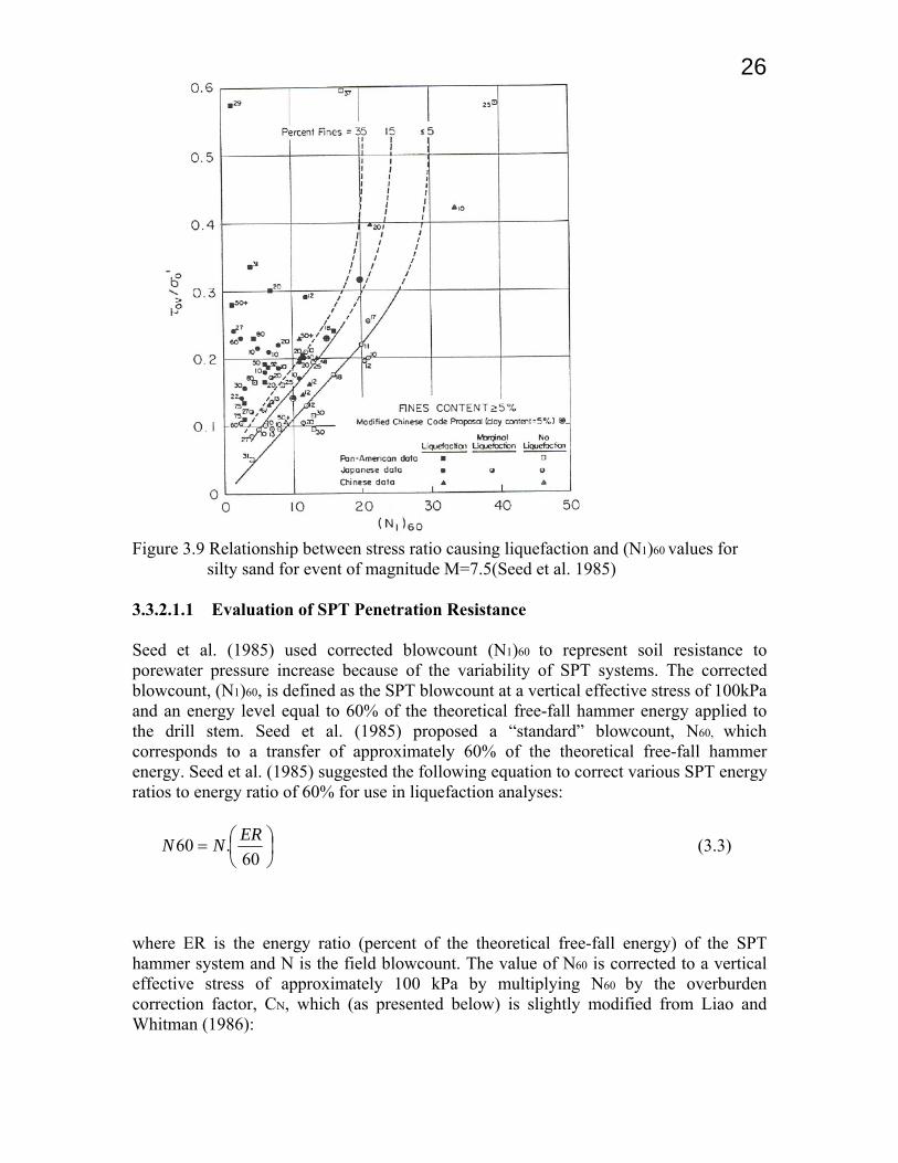
26

Figure 3.9 Relationship between stress ratio causing liquefaction and (N1)60 values for silty sand for event of magnitude M=7.5(Seed et al. 1985) 3.3.2.1.1 Evaluation of SPT Penetration Resistance Seed et al. (1985) used corrected blowcount (N1)60 to represent soil resistance to porewater pressure increase because of the variability of SPT systems. The corrected blowcount, (N1)60, is defined as the SPT blowcount at a vertical effective stress of 100kPa and an energy level equal to 60% of the theoretical free-fall hammer energy applied to the drill stem. Seed et al. (1985) proposed a “standard” blowcount, N60, which corresponds to a transfer of approximately 60% of the theoretical free-fall hammer energy. Seed et al. (1985) suggested the following equation to correct various SPT energy ratios to energy ratio of 60% for use in liquefaction analyses:

⎟⎠⎞

⎜⎝⎛=

60.60 ERNN (3.3)

where ER is the energy ratio (percent of the theoretical free-fall energy) of the SPT hammer system and N is the field blowcount. The value of N60 is corrected to a vertical effective stress of approximately 100 kPa by multiplying N60 by the overburden correction factor, CN, which (as presented below) is slightly modified from Liao and Whitman (1986):

27

n

voPaNCnNN ⎟

⎠⎞

⎜⎝⎛==

'.60.6060)1(σ

(3.4)

where Pa is one atmosphere of pressure in the units of σ’vo and n is equal to 0.5 for sands. The value of (N1)60 must then be corrected for borehole diameter, rod length, and sampling spoon configuration (Youd and Idriss 1997). 3.3.2.2 Method Based on the Cone Penetration Test Because the SPT is subject to numerous corrections including energy ratio, overburden correction, borehole diameter, rod length, and sampling method (Youd and Idriss, eds., 1997), several researchers (e.g., Robertson and Campanella 1985, Seed and de Alba 1986, Shibata and Teparaksa 1988, Stark and Olson 1995, etc.), have investigated the use of the cone penetration test to estimate the level ground liquefaction resistance of sandy soils. The CPT has 5 main advantages over the usual combination of boring, sampling and standard penetration testing:

1. it can be more economical to perform than the SPT, which allows a more comprehensive subsurface investigation.

2. the test procedure is simpler, more standardized, and more reproducible than the SPT.

3. it provides a continuous record of penetration resistance throughout a soil deposit, which provides a better description of soil variability and allows thin (greater than 15 cm in thickness) liquefiable sand or silt to be located and properly characterized. This is particularly important in sands and silts because of the natural non-uniformity of these deposits.

4. it avoids the disturbance of ground associated with boring and sampling, particularly that which occurs with Standard Penetration Test (SPT).

5. it is faster by a factor of 10. Based on these advantages, it is desirable to develop relationships between CPT tip resistance and liquefaction resistance, rather relying on a conversion from SPT blowcount to CPT tip resistance to develop CPT based liquefaction resistance relationships. The main reasons why the CPT has not been used extensively for liquefaction assessment are: • The lack of a sample for soil classification and grain size analysis. • A limited amount of CPT based field data pertaining to liquefaction resistance

was available • Limited availability of cone penetration test equipment in some locales.

28During a CPT, an electrical cone on the end of a series of rods is pushed into the ground at a constant rate of 2cm/s. Continuous measurements are made of resistance to penetration of the cone tip (qc) and the frictional resistance (fs), or adhesion, on a surface sleeve set immediately behind the cone end assembly. Measurements can also be made of other soil parameters using more specialized cones such as poer water pressure (piezecone), electrical conductivity, shear wave velocity (seismic cone), and pressuremeter cone. The CPT has three main applications;

1. To determine the soil profile and identify the soil present 2. To interpolate ground conditions between control boreholes. 3. To evaluate the engineering parameters of the soils and to asses the bearing

capacity and settlement of foundations. In this third role, in relation to certain problems, the evaluation is essentially preliminary in nature, preferably supplemented by borings and other tests, either in situ or in the laboratory. In this respect, the CPT provides guidance on the nature of such additional testing, and helps to determine the positions and levels at which in situ tests or sampling should be undertaken. Where the geology is fairly uniform and predictions based on CPT results have been extensively correlated with building performance, the CPT can be used alone in investigation for building foundations. Even in these circumstances it is preferable that CPTs be accompanied by, or followed by, borings for one or more of the following reasons:

1. To assist where there is difficulty in the interpretation of the CPT result. 2. To further investigate layers with relatively low cone resistance. 3. To explore below the maximum depth attainable by CPT. 4. If the project involves excavation, where samples may be required for laboratory

testing and knowledge of ground water levels and permeability is needed. 3.3.2.2.1 Evaluation of CPT ¨Penetration Resistance Penetration resistance from CPT, similar to SPT blowcount, is influenced by soil density, soil structure, cementation, aging, stress state, and stress history, and thus can be used to estimate liquefaction resistance (Robertson and Campenalla 1985). The corrected CPT tip resistance qc1N, is obtained as follows:

21

21

PaqcCq

PaqcNqc =⎟

⎠⎞

⎜⎝⎛= (3.5)

where qc is the measured cone tip penetration resistance; ( )nvoPaCq 'σ= is a correction

for overburden stress; the exponential n is typically equal to 0.5; Pa is a reference pressure in the same units as vo'σ (i.e., Pa=100 kPa if vo'σ is in kPa); and Pa2 is a reference pressure in the same units as qc (i.e., Pa2 =0.1 Mpa if qc is in MPa)

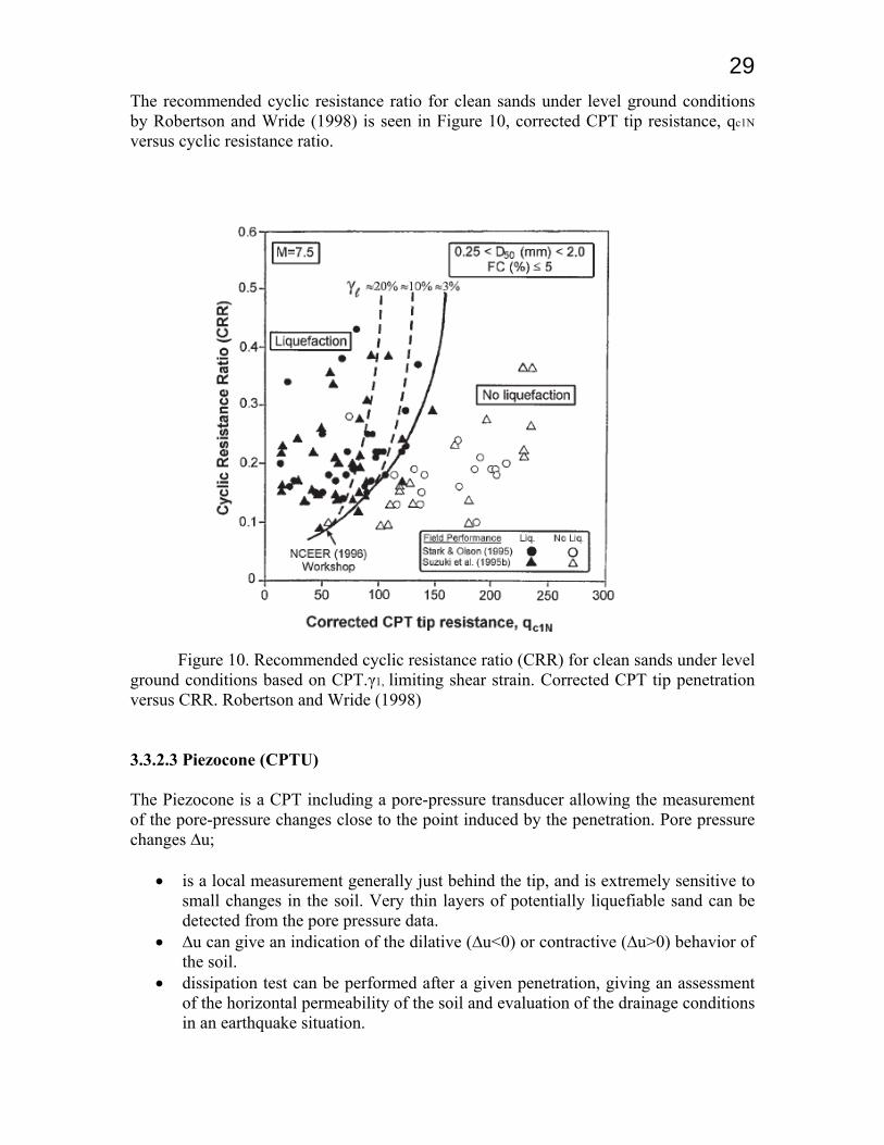
29The recommended cyclic resistance ratio for clean sands under level ground conditions by Robertson and Wride (1998) is seen in Figure 10, corrected CPT tip resistance, qc1N

versus cyclic resistance ratio. Figure 10. Recommended cyclic resistance ratio (CRR) for clean sands under level ground conditions based on CPT.γ1, limiting shear strain. Corrected CPT tip penetration versus CRR. Robertson and Wride (1998) 3.3.2.3 Piezocone (CPTU) The Piezocone is a CPT including a pore-pressure transducer allowing the measurement of the pore-pressure changes close to the point induced by the penetration. Pore pressure changes ∆u;

• is a local measurement generally just behind the tip, and is extremely sensitive to small changes in the soil. Very thin layers of potentially liquefiable sand can be detected from the pore pressure data.

• ∆u can give an indication of the dilative (∆u<0) or contractive (∆u>0) behavior of the soil.

• dissipation test can be performed after a given penetration, giving an assessment of the horizontal permeability of the soil and evaluation of the drainage conditions in an earthquake situation.

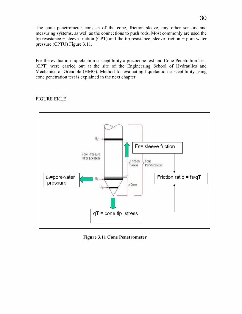
30The cone penetrometer consists of the cone, friction sleeve, any other sensors and measuring systems, as well as the connections to push rods. Most commonly are used the tip resistance + sleeve friction (CPT) and the tip resistance, sleeve friction + pore water pressure (CPTU) Figure 3.11. For the evaluation liquefaction susceptibility a piezocone test and Cone Penetration Test (CPT) were carried out at the site of the Engineering School of Hydraulics and Mechanics of Grenoble (HMG). Method for evaluating liquefaction susceptibility using cone penetration test is explained in the next chapter FIGURE EKLE

Figure 3.11 Cone Penetrometer

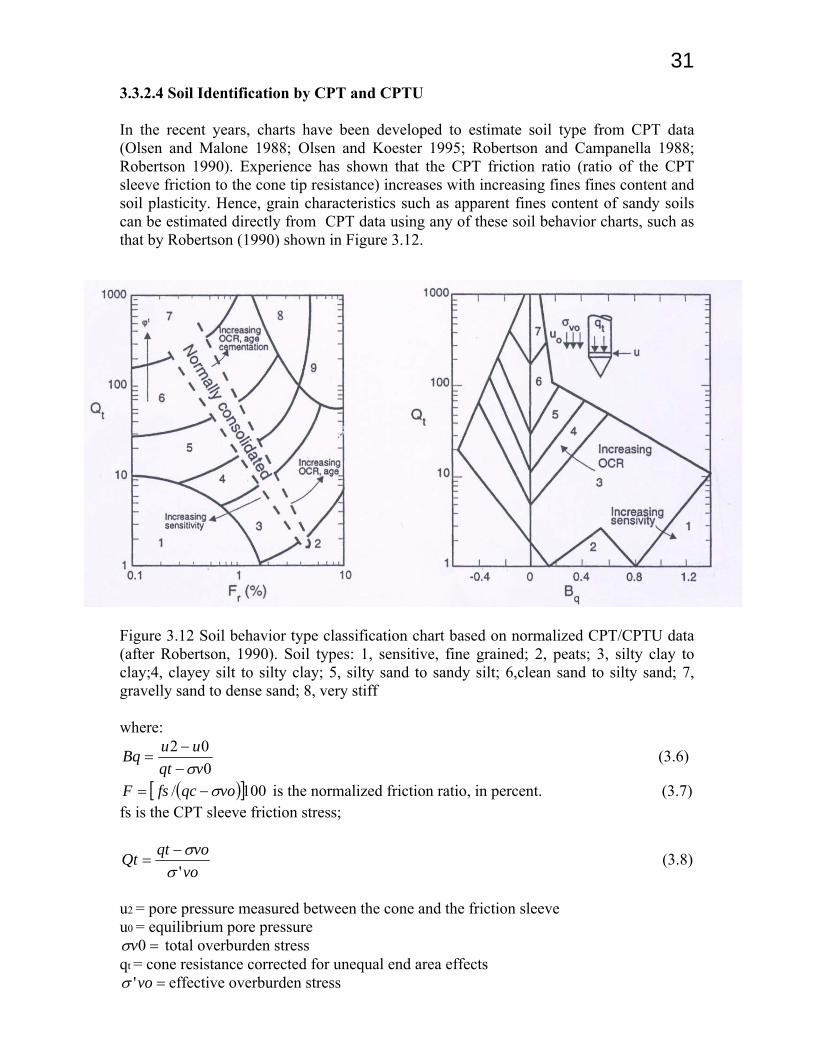
313.3.2.4 Soil Identification by CPT and CPTU In the recent years, charts have been developed to estimate soil type from CPT data (Olsen and Malone 1988; Olsen and Koester 1995; Robertson and Campanella 1988; Robertson 1990). Experience has shown that the CPT friction ratio (ratio of the CPT sleeve friction to the cone tip resistance) increases with increasing fines fines content and soil plasticity. Hence, grain characteristics such as apparent fines content of sandy soils can be estimated directly from CPT data using any of these soil behavior charts, such as that by Robertson (1990) shown in Figure 3.12.

Figure 3.12 Soil behavior type classification chart based on normalized CPT/CPTU data (after Robertson, 1990). Soil types: 1, sensitive, fine grained; 2, peats; 3, silty clay to clay;4, clayey silt to silty clay; 5, silty sand to sandy silt; 6,clean sand to silty sand; 7, gravelly sand to dense sand; 8, very stiff where:

002

vqtuuBqσ−−

= (3.6)

( )[ ]100/ voqcfsF σ−= is the normalized friction ratio, in percent. (3.7) fs is the CPT sleeve friction stress;

vovoqtQt

'σσ−

= (3.8)

u2 = pore pressure measured between the cone and the friction sleeve u0 = equilibrium pore pressure

=0vσ total overburden stress qt = cone resistance corrected for unequal end area effects

=vo'σ effective overburden stress

32

CHAPTER 4 Evaluation of Liquefaction Susceptibility in Grenoble Basin Using Cone Penetration

Test (CPT) 4.1. Seismotectonic Frame of the Grenoble Valley 4.1.1 Geography of the Y-shaped Grenoble Valley Grenoble is settled on Quarternary loose fluvial deposits at the junction of 3 large valleys of the French external Alps (Figure 4.1). This junction mimics the letter Y (the so-called Grenoble Y), with three legs:

1. The N.30-40 trending Gresivaudan valley corresponds to the north-eastern branch of the Y and extends from Grenoble to Montmelian. The Isere River there flows to the SSW. The Combe-de-Savoie Valley continues the Gresivaudan valley north of Montmelian.

2. The N.150 trending north-western branch is called Cluse-de-l’Isere from Grenoble to Moirans. There the Isere Rivers flows to the NW.

3. The N.10 trending leg of the Y corresponds to the plain of the Drac River, spanning 15 km south of Grenoble.

There three valleys delineate three massifs. The Belledone external crystalline massif lays east of the Gresivaudan valley and the Drac plain. The N.30 trending sub alpine sedimentary Chartreuse massif lays between the Gresivaudan and the Cluse-de-l’Isere valleys. The subalpine sedimentary Vercors massif is located SW of the Cluse-de-l’Isere and west of the Drac plain. 4.1.2 Structure of the Isere Valley From 110 km, from Albertville in the NE to Rovon west of the Vercors massif, the Isere valley (Gresivaudan, Cluse-de-l’Isere, basse-Isere) is flat, with slowly decreasing altitudes (330m in Albertville, 211m in Grenoble, 180m in Rovon). Its morphology with asymmetrical inclined sides and longitudinal moraines on the glacial shoulders indicates that glaciers contributed to shape the present topography. These glaciers (Isere glacier, local glaciers of the Belledonne massif, Drac-Romanche glacier) followed the fluvial valley of the Isere River created as early as the end of the Tertiary. The geometry of the glacial through beneath the flat surface constituted by the post-glacial infilling sediments is still poorly known.

33 Figure 4.1 Grenoble topographic and tectonic framework. Light grey: sedimentary Mesozoic cover of Vercors, Chartreuse, Bauges massifs and Belledone border hills. Dark grey with crosses: Paleozoic crystalline basement. Dotted: bas-Dauphine Tertiary and Quaternary depositis. White: Quaternary alluvium of the Isere valley. Thick dashed line: Belledone Border Fault trace. BMF: Belledone Middle Fault

34

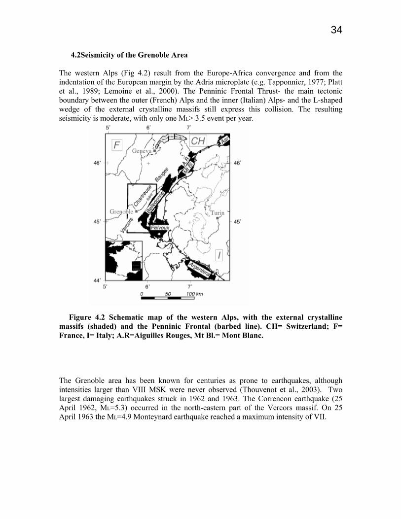
4.2Seismicity of the Grenoble Area The western Alps (Fig 4.2) result from the Europe-Africa convergence and from the indentation of the European margin by the Adria microplate (e.g. Tapponnier, 1977; Platt et al., 1989; Lemoine et al., 2000). The Penninic Frontal Thrust- the main tectonic boundary between the outer (French) Alps and the inner (Italian) Alps- and the L-shaped wedge of the external crystalline massifs still express this collision. The resulting seismicity is moderate, with only one ML> 3.5 event per year. Figure 4.2 Schematic map of the western Alps, with the external crystalline massifs (shaded) and the Penninic Frontal (barbed line). CH= Switzerland; F= France, I= Italy; A.R=Aiguilles Rouges, Mt Bl.= Mont Blanc. The Grenoble area has been known for centuries as prone to earthquakes, although intensities larger than VIII MSK were never observed (Thouvenot et al., 2003). Two largest damaging earthquakes struck in 1962 and 1963. The Correncon earthquake (25 April 1962, ML=5.3) occurred in the north-eastern part of the Vercors massif. On 25 April 1963 the ML=4.9 Monteynard earthquake reached a maximum intensity of VII.

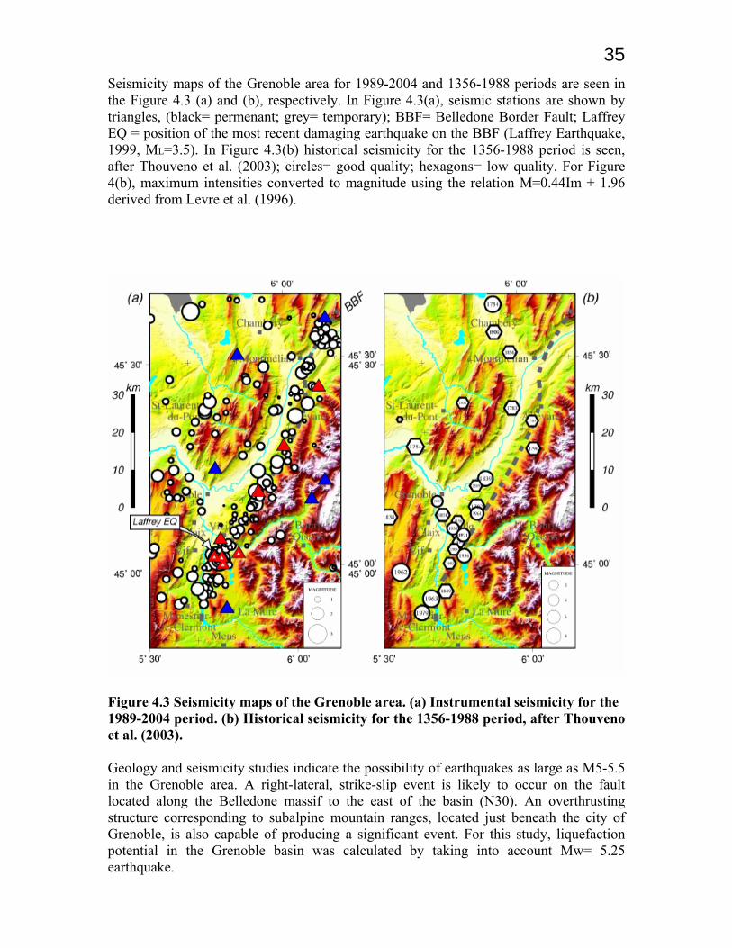
35Seismicity maps of the Grenoble area for 1989-2004 and 1356-1988 periods are seen in the Figure 4.3 (a) and (b), respectively. In Figure 4.3(a), seismic stations are shown by triangles, (black= permenant; grey= temporary); BBF= Belledone Border Fault; Laffrey EQ = position of the most recent damaging earthquake on the BBF (Laffrey Earthquake, 1999, ML=3.5). In Figure 4.3(b) historical seismicity for the 1356-1988 period is seen, after Thouveno et al. (2003); circles= good quality; hexagons= low quality. For Figure 4(b), maximum intensities converted to magnitude using the relation M=0.44Im + 1.96 derived from Levre et al. (1996).

Figure 4.3 Seismicity maps of the Grenoble area. (a) Instrumental seismicity for the 1989-2004 period. (b) Historical seismicity for the 1356-1988 period, after Thouveno et al. (2003). Geology and seismicity studies indicate the possibility of earthquakes as large as M5-5.5 in the Grenoble area. A right-lateral, strike-slip event is likely to occur on the fault located along the Belledone massif to the east of the basin (N30). An overthrusting structure corresponding to subalpine mountain ranges, located just beneath the city of Grenoble, is also capable of producing a significant event. For this study, liquefaction potential in the Grenoble basin was calculated by taking into account Mw= 5.25 earthquake.

36 4.3 Evaluation of the Liquefaction Susceptibility in the Grenoble Basin For the evaluation of liquefaction susceptibility a piezecone test and Cone Penetration Test (CPT) were carried out at the site of the Engineering School of Hydraulics and Mechanics of Grenoble (HMG). CPT and piezecone tests were done until 6.8 meters depth, below which dense gravel layer prevented penetration. Intact samples were obtained by drilling from 1.7 to 2.8 meters and from 3.0 to 4.3 meters. Intact samples are used to obtain cyclic resistance ratio of the soil by cyclic triaxial test. Initially water table is assumed at the depth of 3.6 meters, thus piezecone profile begins at 3.6 meters depth. 11 dissipation tests were carried out at 3.71m, 3.98m, 4.18m, 4.42m, 4.77m, 5.26m, 5.55m, 5.87, 6.19m, 6.32m, 6.68m depths to obtain t50 values. 4.3.1 Evaluation of Liquefaction Susceptibility using Cone Penetration Test For this study, the proposed integrated method by Robertson and Wride (1998) is applied using magnitude-dependent stress reduction factor (rd) and magnitude scaling factor (MSF) which are defined by Idriss and Boulanger (2004) for the evaluation of liquefaction potential. Liquefaction potential in the Grenoble basin was calculated by taking into account Mw= 5.25 earthquake. The proposed integrated method by Robertson and Wride (1998) is summarized in Figure 4.5 in the form of a flow chart. ∆u and t50 values are obtained using piezecone. ∆u and t50 are the excess pore water pressure due to penetration and, the time in which 50% of the over pore water pressure is dissipated during a dissipation test, respectively. ∆u=u-u0, u0 is the hydrostatic pore water pressure. The CPT cone tip resistance, (qc) and friction ratio (F) are used to estimate soil grain characteristics in terms of “soil behaviour type index” (Ic). Ic was calculated by iteration. The final continuous profile of CRR at N=15 cycles (M=7.5) is calculated from the equivalent clean sand values of qc1N (i.e., (qc1N)cs=Kcqc1N) Cyclic stress ratio for Mw=5.25 earthquake is calculated by using simplified procedure by Seed and Idriss (1971);

rdvovo

ga

voavCSR ⎟

⎠⎞

⎜⎝⎛⎟⎟⎠

⎞⎜⎜⎝

⎛==

'max65.0

' σσ

στ (4.1)

where avτ is the average cyclic shear sress; amax is the maximum horizontal acceleration at the ground surface; g is the acceleration due to the gravity; voσ and vo'σ are the total and effective vertical overburden stresses, respectively; and rd is the stress reduction factor. rd stress reduction coefficient, magnitude scaling coefficient, MSF, cyclic resistance ratio, CRR, soil type index, Ic, and apparent fines content are calculated as explained in the following sections.

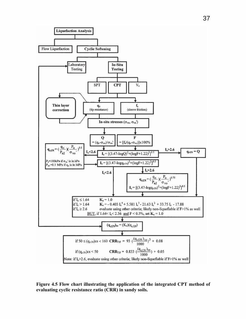
37

Figure 4.5 Flow chart illustrating the application of the integrated CPT method of evaluating cyclic resistance ratio (CRR) in sandy soils.

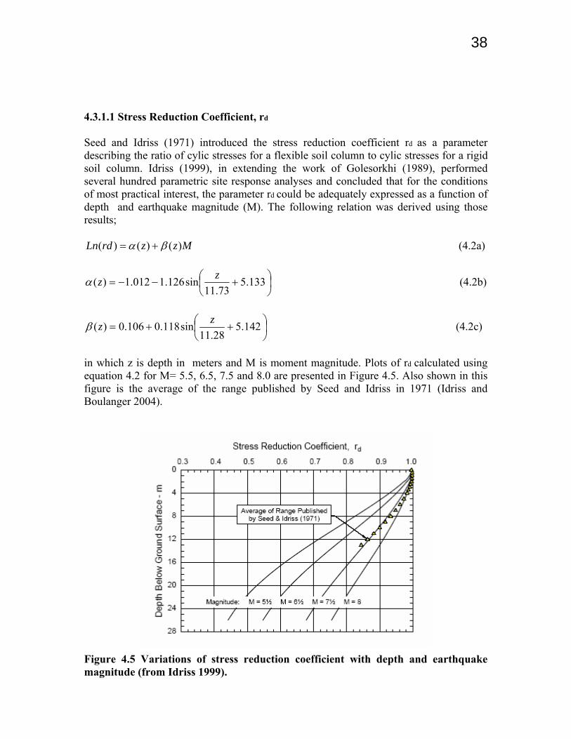
38 4.3.1.1 Stress Reduction Coefficient, rd Seed and Idriss (1971) introduced the stress reduction coefficient rd as a parameter describing the ratio of cylic stresses for a flexible soil column to cylic stresses for a rigid soil column. Idriss (1999), in extending the work of Golesorkhi (1989), performed several hundred parametric site response analyses and concluded that for the conditions of most practical interest, the parameter rd could be adequately expressed as a function of depth and earthquake magnitude (M). The following relation was derived using those results;

MzzrdLn )()()( βα += (4.2a)

⎟⎠⎞

⎜⎝⎛ +−−= 133.5

73.11sin126.1012.1)( zzα (4.2b)

⎟⎠⎞

⎜⎝⎛ ++= 142.5

28.11sin118.0106.0)( zzβ (4.2c)

in which z is depth in meters and M is moment magnitude. Plots of rd calculated using equation 4.2 for M= 5.5, 6.5, 7.5 and 8.0 are presented in Figure 4.5. Also shown in this figure is the average of the range published by Seed and Idriss in 1971 (Idriss and Boulanger 2004). Figure 4.5 Variations of stress reduction coefficient with depth and earthquake magnitude (from Idriss 1999).

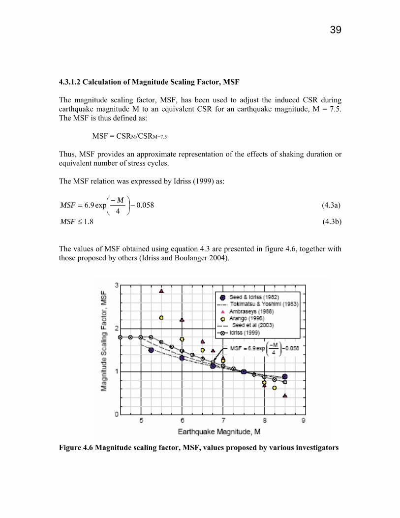
39 4.3.1.2 Calculation of Magnitude Scaling Factor, MSF The magnitude scaling factor, MSF, has been used to adjust the induced CSR during earthquake magnitude M to an equivalent CSR for an earthquake magnitude, M = 7.5. The MSF is thus defined as: MSF = CSRM/CSRM=7.5

Thus, MSF provides an approximate representation of the effects of shaking duration or equivalent number of stress cycles. The MSF relation was expressed by Idriss (1999) as:

058.04

exp9.6 −⎟⎠⎞

⎜⎝⎛ −=

MMSF (4.3a)

8.1≤MSF (4.3b) The values of MSF obtained using equation 4.3 are presented in figure 4.6, together with those proposed by others (Idriss and Boulanger 2004). Figure 4.6 Magnitude scaling factor, MSF, values proposed by various investigators

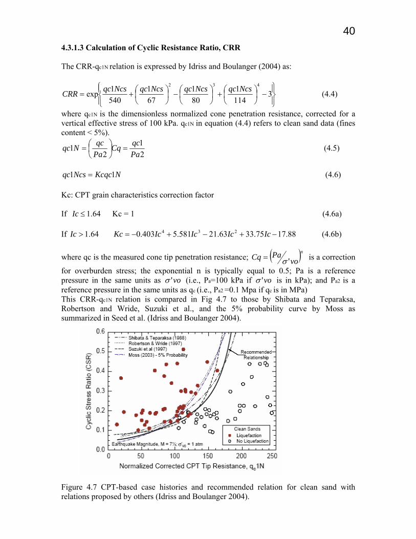
404.3.1.3 Calculation of Cyclic Resistance Ratio, CRR The CRR-qc1N relation is expressed by Idriss and Boulanger (2004) as:

⎪⎭

⎪⎬⎫

⎪⎩

⎪⎨⎧

−⎟⎠⎞

⎜⎝⎛+⎟

⎠⎞

⎜⎝⎛−⎟

⎠⎞

⎜⎝⎛+= 3

1141

801

671

5401exp

432 NcsqcNcsqcNcsqcNcsqcCRR (4.4)

where qc1N is the dimensionless normalized cone penetration resistance, corrected for a vertical effective stress of 100 kPa. qc1N in equation (4.4) refers to clean sand data (fines content < 5%).

21

21

PaqcCq

PaqcNqc =⎟

⎠⎞

⎜⎝⎛= (4.5)

NKcqcNcsqc 11 = (4.6)

Kc: CPT grain characteristics correction factor If 64.1≤Ic Kc = 1 (4.6a) If 64.1>Ic 88.1775.3363.21581.5403.0 234 −+−+−= IcIcIcIcKc (4.6b)

where qc is the measured cone tip penetration resistance; ( )nvoPaCq 'σ= is a correction

for overburden stress; the exponential n is typically equal to 0.5; Pa is a reference pressure in the same units as vo'σ (i.e., Pa=100 kPa if vo'σ is in kPa); and Pa2 is a reference pressure in the same units as qc (i.e., Pa2 =0.1 Mpa if qc is in MPa) This CRR-qc1N relation is compared in Fig 4.7 to those by Shibata and Teparaksa, Robertson and Wride, Suzuki et al., and the 5% probability curve by Moss as summarized in Seed et al. (Idriss and Boulanger 2004). Figure 4.7 CPT-based case histories and recommended relation for clean sand with relations proposed by others (Idriss and Boulanger 2004).

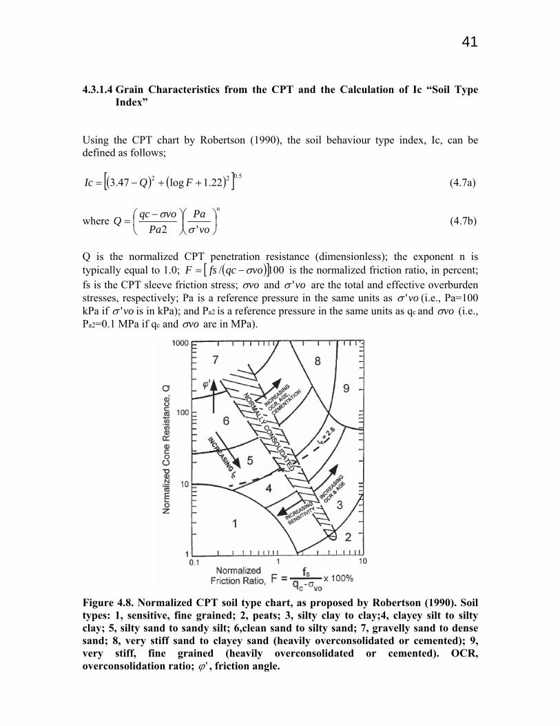
41 4.3.1.4 Grain Characteristics from the CPT and the Calculation of Ic “Soil Type

Index” Using the CPT chart by Robertson (1990), the soil behaviour type index, Ic, can be defined as follows;

( ) ( )[ ] 5.022 22.1log47.3 ++−= FQIc (4.7a)

where n

voPa

PavoqcQ ⎟

⎠⎞

⎜⎝⎛⎟⎠⎞

⎜⎝⎛ −

='2 σ

σ (4.7b)

Q is the normalized CPT penetration resistance (dimensionless); the exponent n is typically equal to 1.0; ( )[ ]100/ voqcfsF σ−= is the normalized friction ratio, in percent; fs is the CPT sleeve friction stress; voσ and vo'σ are the total and effective overburden stresses, respectively; Pa is a reference pressure in the same units as vo'σ (i.e., Pa=100 kPa if vo'σ is in kPa); and Pa2 is a reference pressure in the same units as qc and voσ (i.e., Pa2=0.1 MPa if qc and voσ are in MPa). Figure 4.8. Normalized CPT soil type chart, as proposed by Robertson (1990). Soil types: 1, sensitive, fine grained; 2, peats; 3, silty clay to clay;4, clayey silt to silty clay; 5, silty sand to sandy silt; 6,clean sand to silty sand; 7, gravelly sand to dense sand; 8, very stiff sand to clayey sand (heavily overconsolidated or cemented); 9, very stiff, fine grained (heavily overconsolidated or cemented). OCR, overconsolidation ratio; 'ϕ , friction angle.

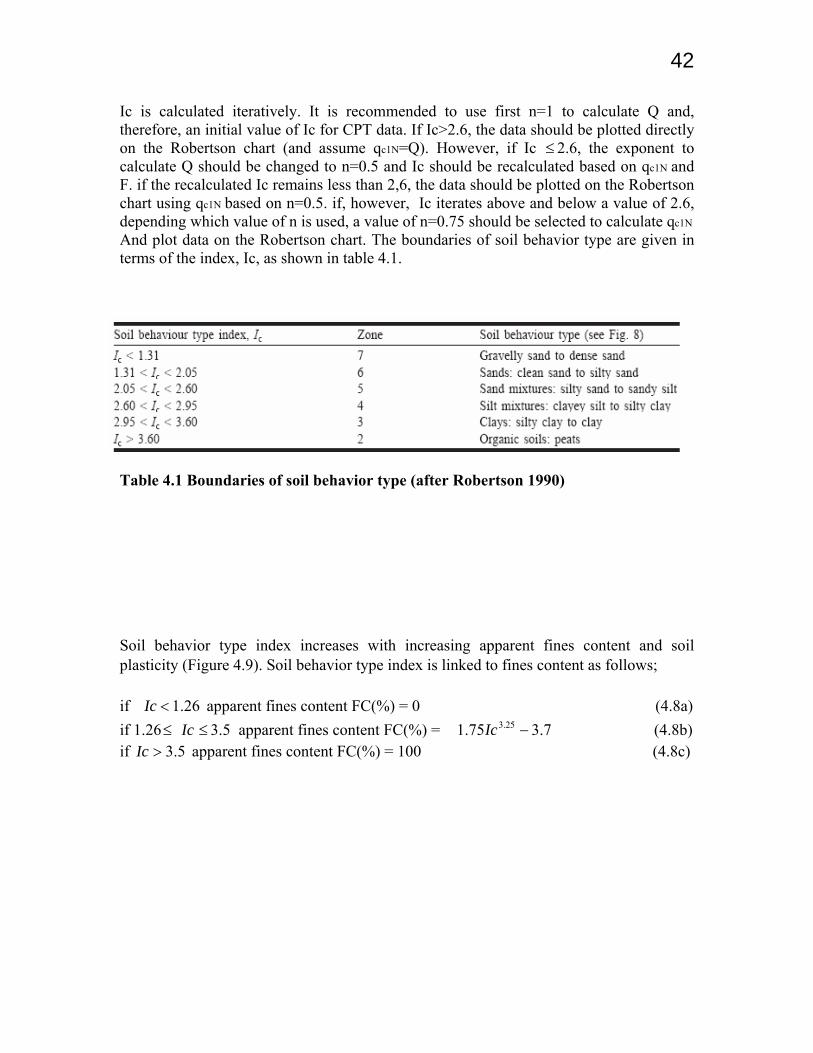
42 Ic is calculated iteratively. It is recommended to use first n=1 to calculate Q and, therefore, an initial value of Ic for CPT data. If Ic>2.6, the data should be plotted directly on the Robertson chart (and assume qc1N=Q). However, if Ic ≤ 2.6, the exponent to calculate Q should be changed to n=0.5 and Ic should be recalculated based on qc1N and F. if the recalculated Ic remains less than 2,6, the data should be plotted on the Robertson chart using qc1N based on n=0.5. if, however, Ic iterates above and below a value of 2.6, depending which value of n is used, a value of n=0.75 should be selected to calculate qc1N

And plot data on the Robertson chart. The boundaries of soil behavior type are given in terms of the index, Ic, as shown in table 4.1.

Table 4.1 Boundaries of soil behavior type (after Robertson 1990) Soil behavior type index increases with increasing apparent fines content and soil plasticity (Figure 4.9). Soil behavior type index is linked to fines content as follows; if 26.1<Ic apparent fines content FC(%) = 0 (4.8a) if 1.26≤ Ic ≤ 3.5 apparent fines content FC(%) = 7.375.1 25.3 −Ic (4.8b) if 5.3>Ic apparent fines content FC(%) = 100 (4.8c)

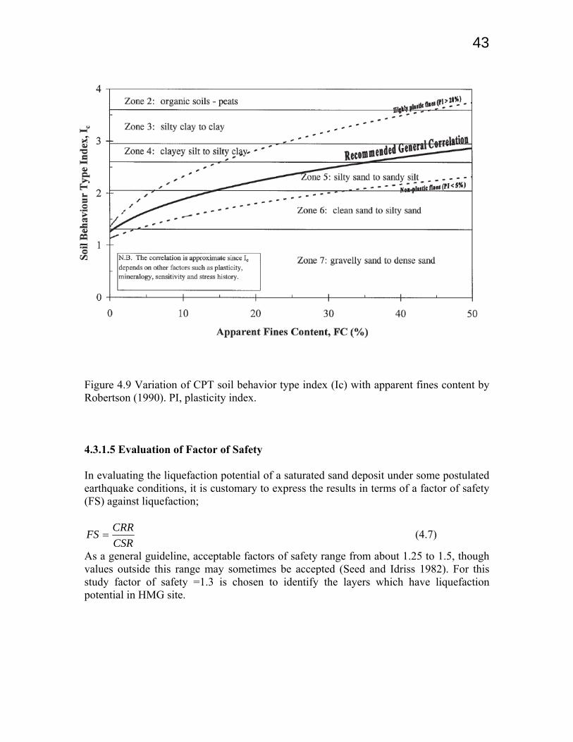
43

Figure 4.9 Variation of CPT soil behavior type index (Ic) with apparent fines content by Robertson (1990). PI, plasticity index. 4.3.1.5 Evaluation of Factor of Safety In evaluating the liquefaction potential of a saturated sand deposit under some postulated earthquake conditions, it is customary to express the results in terms of a factor of safety (FS) against liquefaction;

CSRCRRFS = (4.7)

As a general guideline, acceptable factors of safety range from about 1.25 to 1.5, though values outside this range may sometimes be accepted (Seed and Idriss 1982). For this study factor of safety =1.3 is chosen to identify the layers which have liquefaction potential in HMG site.

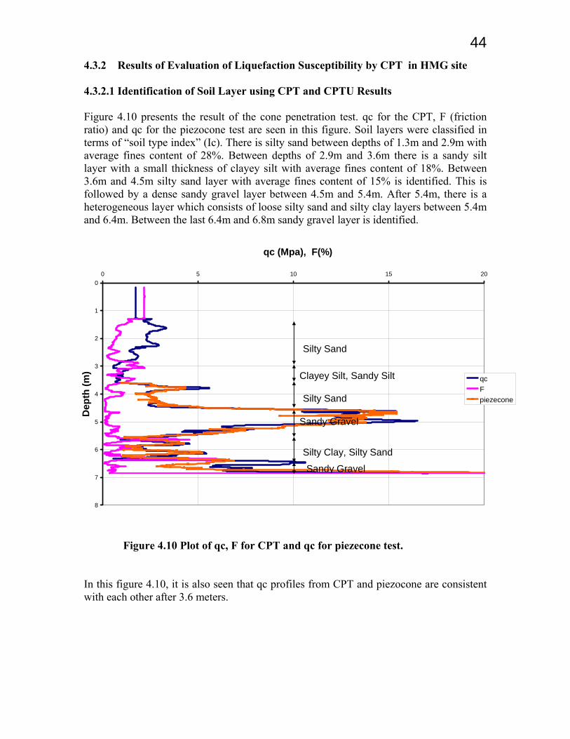
444.3.2 Results of Evaluation of Liquefaction Susceptibility by CPT in HMG site 4.3.2.1 Identification of Soil Layer using CPT and CPTU Results Figure 4.10 presents the result of the cone penetration test. qc for the CPT, F (friction ratio) and qc for the piezocone test are seen in this figure. Soil layers were classified in terms of “soil type index” (Ic). There is silty sand between depths of 1.3m and 2.9m with average fines content of 28%. Between depths of 2.9m and 3.6m there is a sandy silt layer with a small thickness of clayey silt with average fines content of 18%. Between 3.6m and 4.5m silty sand layer with average fines content of 15% is identified. This is followed by a dense sandy gravel layer between 4.5m and 5.4m. After 5.4m, there is a heterogeneous layer which consists of loose silty sand and silty clay layers between 5.4m and 6.4m. Between the last 6.4m and 6.8m sandy gravel layer is identified.

Figure 4.10 Plot of qc, F for CPT and qc for piezecone test. In this figure 4.10, it is also seen that qc profiles from CPT and piezocone are consistent with each other after 3.6 meters.

qc (Mpa), F(%)

0

1

2

3

4

5

6

7

8

0 5 10 15 20

Dep

th (m

)

qcFpiezecone

Silty Sand

Clayey Silt, Sandy Silt

Silty Sand

Sandy Gravel

Silty Clay, Silty Sand

Sandy Gravel

45

Bq-Qt

0

50

100

150

200

250

300

-0.04 -0.02 0 0.02 0.04 0.06 0.08 0.1 0.12 0.14

Bq

Qt

Depth 3.6m-4.5mDepth 4.5m-5.4mDept 5.6m-6.4mDepth 6.4m-6.8m

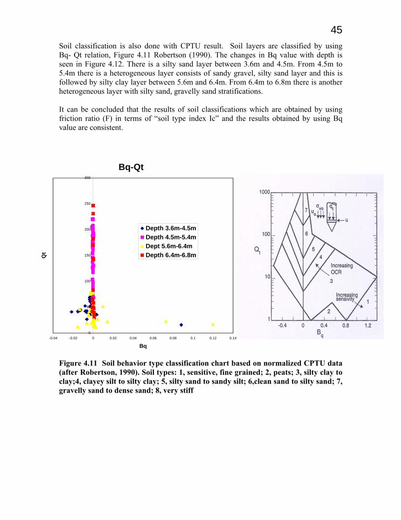
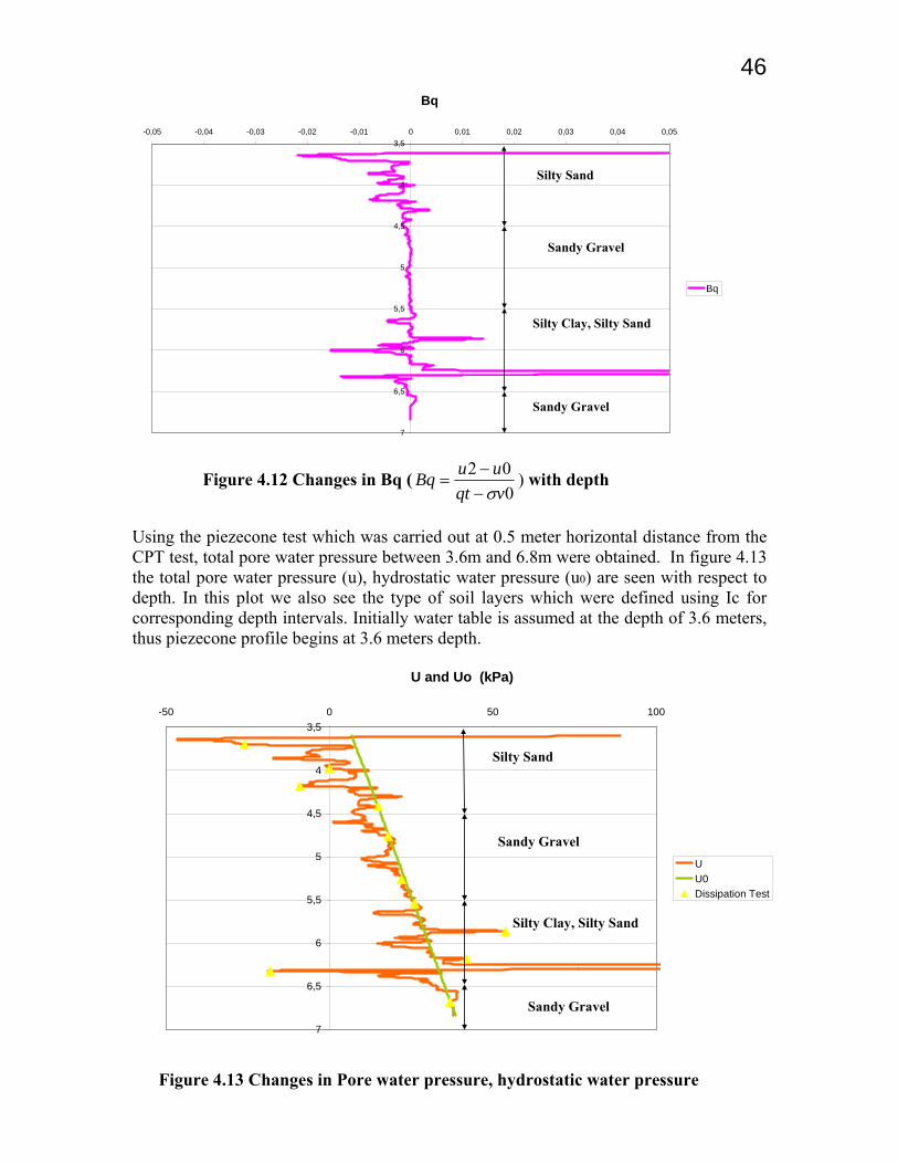
Soil classification is also done with CPTU result. Soil layers are classified by using Bq- Qt relation, Figure 4.11 Robertson (1990). The changes in Bq value with depth is seen in Figure 4.12. There is a silty sand layer between 3.6m and 4.5m. From 4.5m to 5.4m there is a heterogeneous layer consists of sandy gravel, silty sand layer and this is followed by silty clay layer between 5.6m and 6.4m. From 6.4m to 6.8m there is another heterogeneous layer with silty sand, gravelly sand stratifications. It can be concluded that the results of soil classifications which are obtained by using friction ratio (F) in terms of “soil type index Ic” and the results obtained by using Bq value are consistent.

Figure 4.11 Soil behavior type classification chart based on normalized CPTU data (after Robertson, 1990). Soil types: 1, sensitive, fine grained; 2, peats; 3, silty clay to clay;4, clayey silt to silty clay; 5, silty sand to sandy silt; 6,clean sand to silty sand; 7, gravelly sand to dense sand; 8, very stiff

46

Figure 4.12 Changes in Bq (002

vqtuuBqσ−−

= ) with depth

Using the piezecone test which was carried out at 0.5 meter horizontal distance from the CPT test, total pore water pressure between 3.6m and 6.8m were obtained. In figure 4.13 the total pore water pressure (u), hydrostatic water pressure (u0) are seen with respect to depth. In this plot we also see the type of soil layers which were defined using Ic for corresponding depth intervals. Initially water table is assumed at the depth of 3.6 meters, thus piezecone profile begins at 3.6 meters depth.

Figure 4.13 Changes in Pore water pressure, hydrostatic water pressure

U and Uo (kPa)

3,5

4

4,5

5

5,5

6

6,5

7

-50 0 50 100

UU0Dissipation Test

Silty Sand

Sandy Gravel

Silty Clay, Silty Sand

Sandy Gravel

Bq

3,5

4

4,5

5

5,5

6

6,5

7

-0,05 -0,04 -0,03 -0,02 -0,01 0 0,01 0,02 0,03 0,04 0,05

Bq

Silty Sand

Sandy Gravel

Silty Clay, Silty Sand

Sandy Gravel

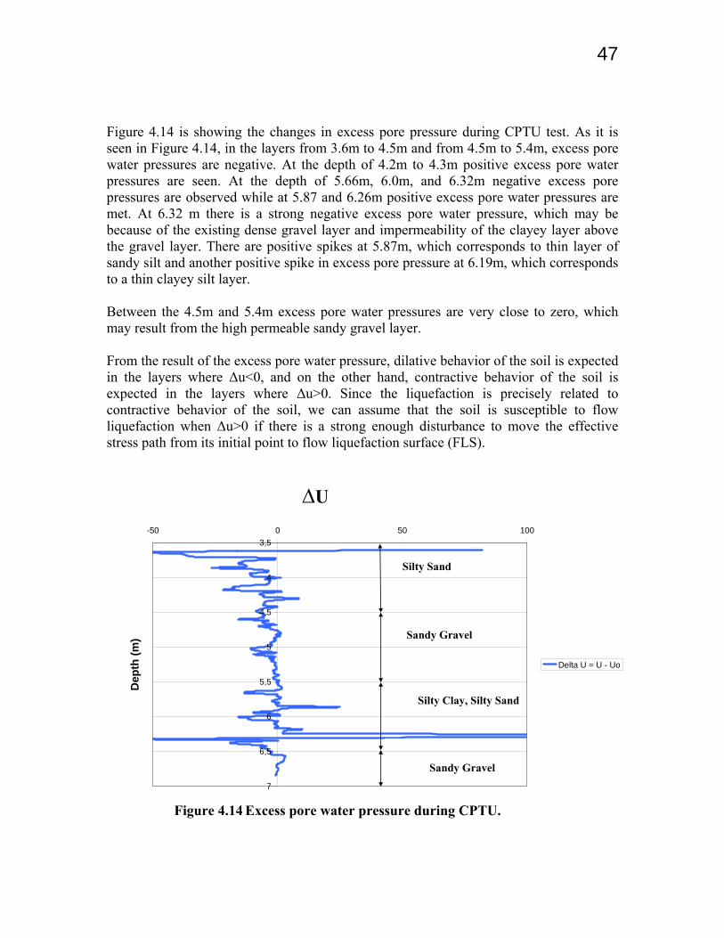
47 Figure 4.14 is showing the changes in excess pore pressure during CPTU test. As it is seen in Figure 4.14, in the layers from 3.6m to 4.5m and from 4.5m to 5.4m, excess pore water pressures are negative. At the depth of 4.2m to 4.3m positive excess pore water pressures are seen. At the depth of 5.66m, 6.0m, and 6.32m negative excess pore pressures are observed while at 5.87 and 6.26m positive excess pore water pressures are met. At 6.32 m there is a strong negative excess pore water pressure, which may be because of the existing dense gravel layer and impermeability of the clayey layer above the gravel layer. There are positive spikes at 5.87m, which corresponds to thin layer of sandy silt and another positive spike in excess pore pressure at 6.19m, which corresponds to a thin clayey silt layer. Between the 4.5m and 5.4m excess pore water pressures are very close to zero, which may result from the high permeable sandy gravel layer. From the result of the excess pore water pressure, dilative behavior of the soil is expected in the layers where ∆u<0, and on the other hand, contractive behavior of the soil is expected in the layers where ∆u>0. Since the liquefaction is precisely related to contractive behavior of the soil, we can assume that the soil is susceptible to flow liquefaction when ∆u>0 if there is a strong enough disturbance to move the effective stress path from its initial point to flow liquefaction surface (FLS). ∆U

Figure 4.14 Excess pore water pressure during CPTU.

3,5

4

4,5

5

5,5

6

6,5

7

-50 0 50 100

Dep

th (m

)

Delta U = U - Uo

Silty Sand

Sandy Gravel

Silty Clay, Silty Sand

Sandy Gravel

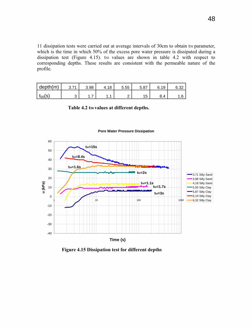
48 11 dissipation tests were carried out at average intervals of 30cm to obtain t50 parameter, which is the time in which 50% of the excess pore water pressure is dissipated during a dissipation test (Figure 4.15). t50 values are shown in table 4.2 with respect to corresponding depths. These results are consistent with the permeable nature of the profile. depth(m) 3.71 3.98 4.18 5.55 5.87 6.19 6.32

t50(s) 3 1.7 1.1 2 15 8.4 1.6 Table 4.2 t50 values at different depths.

Figure 4.15 Dissipation test for different depths

Pore Water Pressure Dissipation

-40

-30

-20

-10

0

10

20

30

40

50

60

1 10 100 1000

Time (s)

u (k

Pa)

3,71 Silty Sand3,98 Silty Sand4,18 Silty Sand5,55 Silty Clay5,87 Silty Clay6,19 Silty Clay6,32 Silty Clay

t50=3s

t50=1.7st50=1.1s

t50=2s

t50=15s

t50=8.4s

t50=1.6s

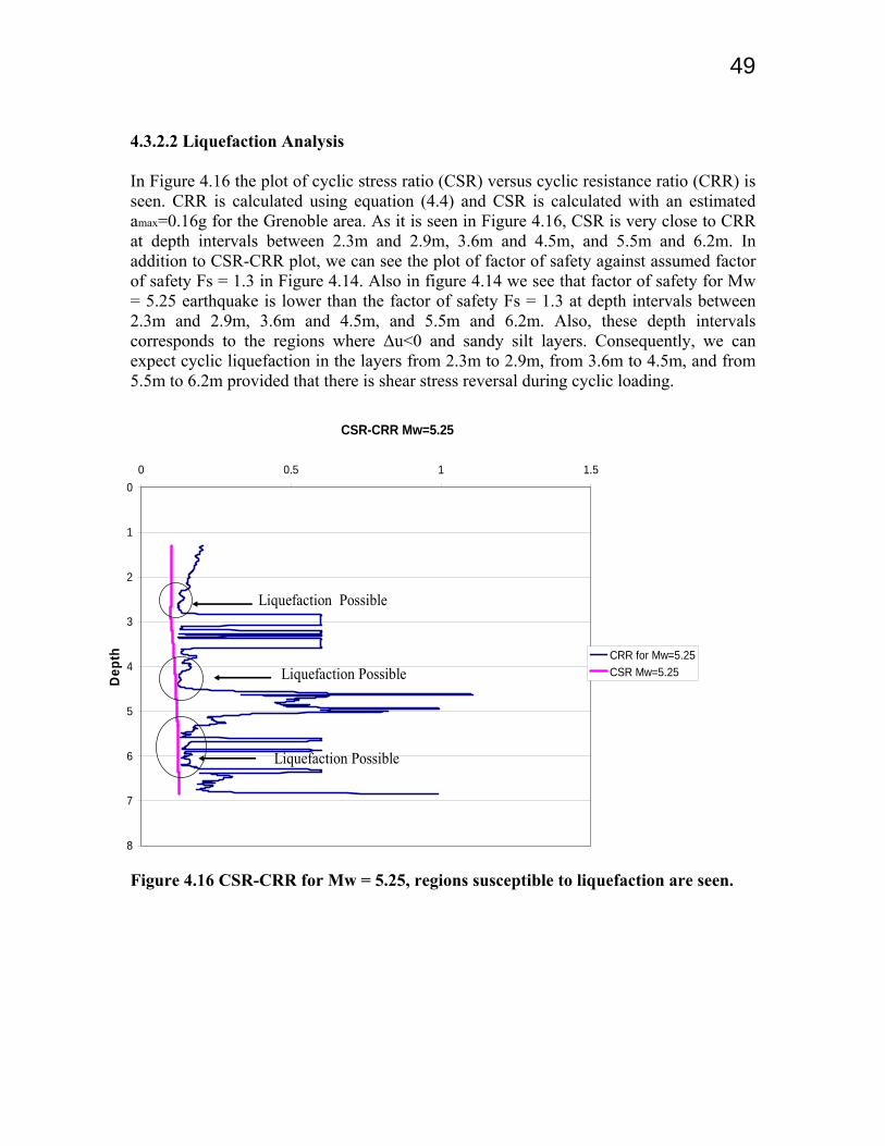
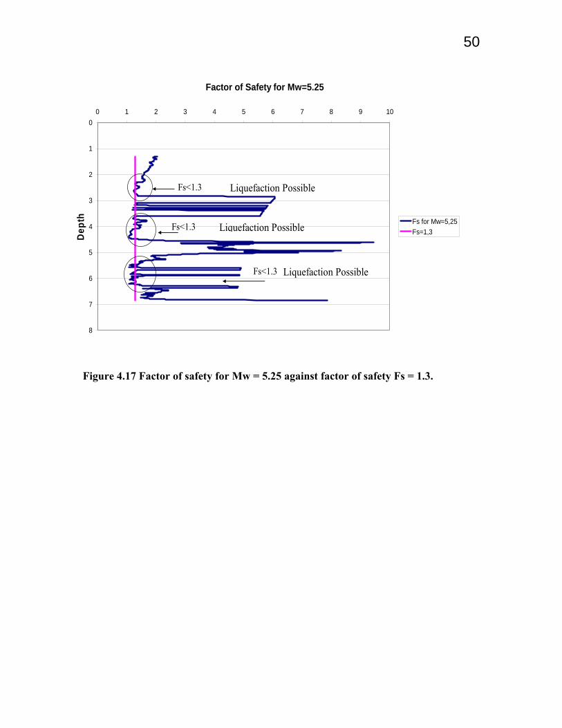
49 4.3.2.2 Liquefaction Analysis In Figure 4.16 the plot of cyclic stress ratio (CSR) versus cyclic resistance ratio (CRR) is seen. CRR is calculated using equation (4.4) and CSR is calculated with an estimated amax=0.16g for the Grenoble area. As it is seen in Figure 4.16, CSR is very close to CRR at depth intervals between 2.3m and 2.9m, 3.6m and 4.5m, and 5.5m and 6.2m. In addition to CSR-CRR plot, we can see the plot of factor of safety against assumed factor of safety Fs = 1.3 in Figure 4.14. Also in figure 4.14 we see that factor of safety for Mw = 5.25 earthquake is lower than the factor of safety Fs = 1.3 at depth intervals between 2.3m and 2.9m, 3.6m and 4.5m, and 5.5m and 6.2m. Also, these depth intervals corresponds to the regions where ∆u<0 and sandy silt layers. Consequently, we can expect cyclic liquefaction in the layers from 2.3m to 2.9m, from 3.6m to 4.5m, and from 5.5m to 6.2m provided that there is shear stress reversal during cyclic loading.

Figure 4.16 CSR-CRR for Mw = 5.25, regions susceptible to liquefaction are seen.

CSR-CRR Mw=5.25

0

1

2

3

4

5

6

7

8

0 0.5 1 1.5

Dep

th CRR for Mw=5.25CSR Mw=5.25

Liquefaction Possible

Liquefaction Possible

Liquefaction Possible

50

Figure 4.17 Factor of safety for Mw = 5.25 against factor of safety Fs = 1.3.

Factor of Safety for Mw=5.25

0

1

2

3

4

5

6

7

8

0 1 2 3 4 5 6 7 8 9 10

Dep

th Fs for Mw=5,25Fs=1,3

Fs<1.3

Fs<1.3

Fs<1.3

Liquefaction Possible

Liquefaction Possible

Liquefaction Possible