Dissertation submitted to the

Dissertation

submitted to the

Combined Faculty of Natural Sciences and Mathematics

of Heidelberg University, Germany

for the degree of

Doctor of Natural Sciences

Put forward by

Tom Segal

born in: Tel Aviv, Israel

Oral examination: 17.10.2019

Mass Measurements of Neon Isotopes at THe-Trap

Referees: Klaus Blaum

Wolfgang Quint

Präzisions-Massenmessungen von Neonisotopen an THe-Trap – ZUSAMMENFASSUNG THe-Trap ist ein Penningfallen Experiment zur Präzisionsmassenbestimmung am Max-Planck- Institut für Kernphysik in Heidelberg, Deutschland. Für das Datenerfassungssystem wurden ein neues Python-Program und eine neue PHP-Website entwickelt. Unter Verwendung eines Lock-In Amplifiers wurde ein neues Locksystem implementiert. Ein Gaseintrittssystem wurde entwickelt und verwendet, um die hochgeladenen Neon-Isotope 20Ne8+

und 22Ne7+ Neon zu

erzeugen und in der Penningfalle einzufangen. Ihre Masse wurde gegen ein 12C Referenzion

gemessen. Die 20Ne-Masse wurde mit einer relativen Messunsicherheit von 5.8 ⋅ 10-10 bestimmt.

Diese befindet sich innerhalb einer Standardabweichung mit dem Literaturwert mit einer

Unsicherheit von 8.4 ⋅ 10-11 im Einklang. Die 22Ne Masse wurde mit einer relative

Messunsicherheit von 7.7 ⋅ 10-10 gemessen. Diese befindet sich innerhalb fünf

Standardabweichungen im Vergleich zur Messunsicherheit des Literaturwerts, 8.2 ⋅ 10-10.

Aufgrund der langen Messdauer ist die Messunsicherheit jeweils von zeitlichen Variationen des Magnetfelds limitiert. Das leichte Edelgas Neon gehört zum “Backbone of the Atomic Mass Evaluation”, weshalb es als Bezugsmasse nützlich ist. Die Verbesserung der relativen Neonmessunsicherheit kann also die relative Messunsicherheit von Messungen verbessern, die Neon als Bezugsmasse verwenden.

Mass Measurements of Neon Isotopes at THe-Trap - ABSTRACT

THe-Trap is a Penning-trap experiment for precision mass measurements located at the Max Planck Institute for Nuclear Physics in Heidelberg, Germany. A new python program and PHP website were created for the data acquisition system and a new lock system was developed using a Lock-In Amplifier. A gas injection system was developed and used for injecting and trapping neon isotopes 20Ne8+

and 22Ne7+ . Their masses were then measured with the use of

12C4+ as reference ions. The 20Ne mass was measured with a relative uncertainty of 5.8 ⋅ 10-10

and is within one standard deviation in comparison to the literature value, which has a relative

uncertainty of 8.4 ⋅ 10-11. The 22Ne mass was measured with a relative uncertainty of 7.7 ⋅ 10-10

and is at a discrepancy of five standard deviations in comparison to the literature value, which

has a relative uncertainty of 8.2 ⋅ 10-10. The relative uncertainties of both measurements are

limited by temporal variations of the magnetic field due to the long measurement times. Being a light noble gas, neon is a part of the “Backbone of the Atomic Mass Evaluation”, such that it is useful as a reference mass. Improving the mass uncertainty of neon can therefore improve the uncertainty of measurements using it as a reference.

“The ability to observe without evaluating is the highest form of intelligence.”

- Jiddu Krishnamurti

“We miss the real by lack of attention and create the unreal by excess of imagination.” - Nisargadatta Maharaj

C O N T E N T S

1 motivation 1

1.1 The Neutrino Mass 1

1.2 The Atomic Mass Evaluation (AME) 4

1.3 Neon Masses 4

1.4 Thesis Layout 5

2 penning-trap theory 7

2.1 Charged Particle Motion in a Penning-Trap 7

2.2 Penning-Trap Geometry 9

2.3 Measurement of the Trapped Particle’s Signal 11

2.3.1 Description of The Image Current 12

2.3.2 Detection of the Image Current 12

2.3.3 The Driven Penning-Trap as a Driven Series RLC Circuit 14

2.3.4 The Detailed Detection Circuit 16

2.4 Expansion of the Electrostatic Potential 18

2.5 Excitations and Couplings 20

2.5.1 Drive signals 20

2.5.2 Coupling Signals 21

2.6 Systematic Shifts 22

2.6.1 Electric Field Shifts 22

2.6.2 Magnetic Field Shift - B2 25

2.6.3 Mixed Shift - C1B1 26

2.6.4 THe-Trap Shifts 26

3 the experimental setup 29

3.1 The Magnet 29

3.1.1 The Repair of the Magnet 32

3.1.2 Shimming the Magnet 32

3.1.3 Shielding Factor Measurements 33

3.2 The Trap Tower 34

3.2.1 The Gas Inlet System 34

3.3 The Stabilization System 34

3.3.1 New Data Acquisition Program - “PyEnvDAQ” 38

3.3.2 New Group Website - “THe-Website” 38

3.4 Loading and Manipulating Ions 38

3.4.1 Locking and detecting the Axial Mode 38

3.4.2 Detecting the Radial Modes 43

4 neon mass measurements 47

4.1 Loading a Single Ion 47

ix

4.2 Pulsing the radial modes to roughly determine the Ion Frequencies 48

4.3 Lock Phase Calibration and Locking the Ion 48

4.4 Aligning the Trap 49

4.5 Radial and Axial Calibration Measurements 50

4.6 Magnetron and Modified Cyclotron Calibration Measurements 50

4.7 Axial Calibration Measurements 54

4.8 The Measurement Method - “Sweeps” 56

4.9 Calculating the Systematic Shifts 60

4.10 Data Analysis 61

4.11 Results 61

4.11.1 The 20Ne8+ Measurement 62

4.11.2 The 22Ne7+ Measurement 62

5 concluding remarks 63

a appendix 65

a.1 THe-Trap Parameters 65

a.2 Expansion of the Electrostatic Potential 66

a.3 Driving and Coupling the Modes 67

a.4 Systematic Shifts - Formulas not used in the Thesis 68

a.4.1 The Ctotal 4 and Ctotal 6 Shifts 68

a.4.2 Image Charge Shift 68

a.4.3 Trap Tilt 68

a.4.4 Magnetic Field Shift - B2 69

Bibliography 71

b acknowledgments 79

x

L I S T O F F I G U R E S

Figure 1.1 The kinetic energy spectrum of the electron emitted in the β-decay oftritium. 2

Figure 1.2 Relative uncertainties of the Q-value of the Tritium-He beta decay as afunction of time. 3

Figure 1.3 Discrepancy between measurements of light ion masses. 4

Figure 2.1 The trajectory of a charged particle in a Penning-trap. 10

Figure 2.2 Half of a hyperbolic Penning-trap with an impedance component con-nected between the endcaps for image current detection. 13

Figure 2.3 The image charge created by an oscillating trapped ion in a Penning-trapis equivalent to a series LC circuit. 15

Figure 2.4 The full Penning-trap detection circuit. 16

Figure 3.1 The magnet. 30

Figure 3.2 The magnet’s relative magnetic field decay rate in ppt/h. 31

Figure 3.3 The results of shimming the magnet. 33

Figure 3.4 Shielding factor measurements. 35

Figure 3.5 The trap tower and the two traps. 36

Figure 3.6 The gas inlet system. 37

Figure 3.7 The Stabilization System 39

Figure 3.8 The new data acquisition program - “PyEnvDAQ”. 40

Figure 3.9 The new group website, “THe-Website”. 41

Figure 3.10 A ring voltage scan revealing trappable ion species in THe-Trap. 42

Figure 3.11 (a) The old axial locking circuit with the “mix2dc box”. (b) the new axiallocking circuit with the Lock-In Amplifier. 44

Figure 4.1 Lock Phase Calibration Measurements 49

Figure 4.2 Magnetron and Modified Cyclotron Calibration Measurements. 51

Figure 4.3 Axial Calibration Measurements. 55

Figure 4.4 The Measurement Method - “Sweeps”. 58

L I S T O F TA B L E S

Table 4.1 Calibration Measurements 57

Table 4.2 Sweep Measurements 59

Table 4.3 Systematic Shifts Results 60

xi

Table 4.4 Neon masses measurement results 62

Table A.1 THe-Trap Parameters 65

xii

1M O T I VAT I O N

Mass spectrometry is the measurement of atomic, nuclear and sub-nuclear masses with highprecision. The Penning trap (see Section 2.1) is the best tool for such measurements [1], asrelative uncertainties of δm

m = 10−9 for short-lived radioactive nuclei [2] and 10−11 for long-livedand stable nuclei [3] can be reached. Precision mass measurements are used for preciselydetermining the values of fundamental constants such as the g-factor of different particles[4], for measurements of so-called reference masses, which are masses used as references indifferent experiments [5], in atomic and nuclear physics to determine nuclear structures, teststrong interaction theories, the electroweak Standard Model and quantum electrodynamics [6],and for measuring or inferring upper bounds on the neutrino masses [7]. Two applications ofrelevance for this thesis will be introduced in more detail in the following.

1.1 the neutrino mass

Neutrinos are electrically-neutral leptons which interact only through the weak nuclear forceand are at least 100,000 times lighter than electrons [8]. They were first predicted in 1930

by Wolfgang Pauli and formulated into a theory by Enrico Fermi as an explanation for theobserved energy spectrum of the electrons e− emitted in the beta-minus decay of neutrons,which corresponded to that of a three-body problem and not to that of a two-body problemas expected. This is due to the presence of the neutrino, which was not yet observed at thattime [9]. There are three neutrino types, also referred to as generations - the electron, tauand muon neutrinos, or six with the anti-neutrinos included. The electron anti-neutrino wasfirst observed in 1956 in the “Cowan-Reines Neutrino Experiment” as a part of the reactionof inverse beta decay in a nuclear reactor νe + p → e+ + n, where νe , p , e+ and n stand forthe electron anti-neutrino, the proton, the positron and the neutron, respectively [10]. Themuon neutrino was observed in 1962 by observing the decay of a pion beam into muonsand neutrinos [11]. The tau neutrino was observed in 2000 as a product of the decay of Ds

mesons, which were created using a proton beam shooting on a tungsten target [12]. Neutrinoshave been observed to oscillate between one another, suggesting both that neutrinos are notmassless, and that the three neutrino types are not mass-eigenstates but superpositions ofthem, as assumed in the Standard Model [13, 14]. The Nobel prize was awarded to TakaakiKajita and Arthur B. McDonald in 2015 for this discovery [15]. The squared mass difference ofneutrino types can be measured from neutrino oscillations, but not the individual masses. Thesum of the three neutrino masses is assumed to be at most 0.39 eV

c2 based on cosmic microwavebackground observations [16] and 0.2 eV

c2 based on an estimate of the influence of neutrinos onnucleon-synthesis following the Big Bang [17, 18]. An overview of such estimates can be found

1

2 motivation

Figure 1.1: The kinetic energy spectrum of the electron emitted in the β-decay of tritium. E0 is the kineticenergy in case neutrinos are massless, as in m (νe) = 0. It is also taken into account that thenon-finite neutrino mass does not only shift the end-point but also changes the shape of thespectrum proportionally to m (νe). Only 2 · 10−13 of the electrons are emitted in the energywindow E0 − 1 eV to E0.

in [19]. The upper bound for the mass of the heaviest anti-neutrino, the electron anti-neutrino,was measured to be m (νe) < 2.3 eV

c2 and later refined to be m (νe) < 2.05 eVc2 [8, 20].

The Karlsruhe Tritium Neutrino Experiment, KATRIN, intends to measure or provide anupper bound of around m (νe) < 0.2 eV

c2 for the electron anti-neutrino mass by measuring theend-point of the energy spectrum of the electrons released in the tritium beta minus decayT → 3He + e + νe. Here T and 3He stand for tritium and for the rare stable helium isotope,respectively. Near the end-point the electrons carry a minimal amount of kinetic energy, suchthat the difference between the measured energy and the Q-value of about 18.6 keV [21]correponds to the neutrino’s rest mass, see Figures 1.1 and 1.2. The measured energy is givenby E = (m (T)−m (3He)−m (νe)) c2 − EEBE − EREC, where the m’s are the masses of tritium,3He and the electron anti-neutrino, respectively, EEBE is the electron binding energy and EREC

is the 3He recoil energy1. Calibration of the end-point with its low count rate is technicallychallenging [7], with a projected uncertainty of 40 meV [23]. Independent measurements areimportant for testing systematic shifts. The current leading measurements have uncertaintiesof 1.2 eV

c2 [24] and 70 meVc2 [25] and differ by two standard deviations.

1 In the mass spectrometry community, the Q-value is defined as the difference between the masses of the motherand daughter nuclei, E = (m (mother)−m (daughter)) c2. However, in the β-spectrometry community, the bindingenergy of the daughter’s missing electron EEBE, the daughter’s recoil energy EREC, calculated from kinematics [22]and the electron anti-neutrino’s mass m (νe) are all taken into account.

1.1 the neutrino mass 3

Figure 1.2: Relative uncertainties of the Q-value of the 3T→3 He β-decay as a function of time gatheredfrom the Atomic Mass Evaluation (AME) [5] by [26]. It can be seen that the relative uncer-tanties gradually decrease due to innovations and improvements in the measurement method.For instance, in 1989 single ion trapping was achieved and two measurement techniqueswere implemented: continous axial detection [27] and “Pulse and Phase” [28]. In 2016 twoions filtered from an injected molecular beam were stored simulatenously in the same trapwith the “parking” method and measured with the “Pulse and Phase” method [25]. Notethat the data points correspond to the AME evaluation dates and not necessarily to the datesof the experiments.

4 motivation

Figure 1.3: Discrepancy between measurements of light ion masses. The HD mass can either be calcu-lated using the 12C ⇐⇒ D [31] and 12C ⇐⇒ H [32] links combined with the bindingenergy of HD [33], or by using the 12C ⇐⇒ 3He link [31] and either the 3He ⇐⇒ HDlink [34, 25] or the 3He ⇐⇒ T and T ⇐⇒ HD links [25]. A five standard deviationsdiscrepancy is revealed by applying all of the links. Based on Figure 1 from [35].

1.2 the atomic mass evaluation (ame)

The AME is a project started in 1970 for gathering values for the atomic masses of all knownnuclei at that time from measurements done by different groups around the world usingmass spectrometers and radioactive decay energy measurements [29, 30]. The precise valuesof atomic masses play an important role in many fields of physics and chemistry, making theAME one of the most cited publications in atomic and nuclear physics and in chemistry. Agroup of precisely-measured, relatively easily-obtainable ions is used as reference masses inmass measurements and for systematic checks of various experiments and is thus referred toas the “backbone” of the AME. Members of this “backbone” are among others, the stable neonisotopes 20,22Ne.

1.3 neon masses

There is a five standard deviations discrepancy between measurements of light ion masses[35], see Figure 1.3. This discrepancy motivated a precision mass measurement of 3,4He. A gasinlet system (see 3.2.1 ) was implemented in preparation for the measurement and neon gaswas used to test this system. Following the successful test, it was decided to perform neonmass measurements, as neon is a part of the “backbone of the AME”, being a readily-availablenoble gas. In this thesis the masses of 20Ne8+ and 22Ne7+ were measured with the use of 12C4+

as a reference ion. The measurement method, results and the concluding remarks are presentedin the rest of the thesis.

1.4 thesis layout 5

1.4 thesis layout

In Chapter 2 the theoretical background required for understanding the experiment is explained:Penning-trap theory and the physics of the detection circuit.In Chapter 3 the experimental setup is described: The magnet including the shielding factormeasurements, the trap tower including the gas inlet system, the LHe pressure and levelstabilization system including the new python control program and the new php website forplotting the recorded data, the field emission point for loading ions and the detection andmanipulation of ions.In Chapter 4 the neon mass measurements are presented: The measurement process, loading asingle ion, calibration measurements, the sweeps measurement method and results.In Chapter 5 concluding remarks regarding the experiment are given.

2P E N N I N G - T R A P T H E O RY

A Penning-trap is a device for storing charged particles. The radial trapping is done by astatic homogeneous magnetic field and the axial trapping by a static quadrupolar electric field.Fundamental properties of the trapped ion, such as its mass, binding energies and magneticmoment or g-factor can then be determined by measuring the ion’s frequencies of motion in thetrap. A quantum description for the motion exists [36], but due to the high quantum numbersof the stored ion used within the experiment carried out here, the motion can be describedclassically, which is easier to intuitively grasp and to numerically simulate [37, 38]. In thischapter, the motion of the charged particle is described clasically with its resulting frequenciesfollowed by a description of the trap geometry in Section 2.2. In Section 2.3 the detection circuitfor detecting the trapped ion’s signal is explained. In Section 2.4 the electrostatic potentialof the Penning-trap is given a more detailed treatment, which is necessary for the remainingsections. In Section 2.5 excitation and coupling signals are explained, and in Section 2.6 a list ofall known shifts and their formulas is provided.

2.1 charged particle motion in a penning-trap

A charged particle in a static homogeneous magnetic field parallel to the z direction, ~B = Bz,experiences a Lorentz force. Substitution into the equation of motion yields

q

vyB

−vxB

0

= m

vx

vy

vz

, (2.1)

where q = ne , m and n are the trapped particle’s charge, mass and charge number, with ebeing the elementary charge. The solutions for the x and y directions is a harmonic motionperpendicular to the magnetic field lines with the cyclotron frequency1

ωc =qBm

, (2.2)

where the index c stands for cyclotron. For the z direction it is obtained that vz = const, suchthat the particle’s motion is bound in the x-y plane but unbound in the z direction. To achieve

1 ω is usually called the angular frequency (ω = 2π f , [ω] = rads ), where f is the frequency ([ f ] = Hz), however in

this thesis it is referred to simply as “frequency”.

7

8 penning-trap theory

trapping in the z direction as well, a electrostatic potential is added. One could naively expecta potential such as φ = 0.5φ2z2 to be sufficient, where φ2 is the potential strength parameter2.However, this potential does not satisfy Laplace’s equation 4φ = 0. To satisfy it, the potentialis modified to be φ = 0.5φ2

(z2 − 0.5ρ2)+ const, where const ≡ 0, such that the electric field

is given by ~E = φ22 (~x +~y− 2~z). However, the additional terms modify the motion in the x-y

plane. The motion in the z direction is still that of an harmonic oscillator with the followingmotion and frequency:

z = Az cos (ωzt + ϕz) , ωz =

√qφ2

m, (2.3)

where Az is a real number denoting the amplitude of the motion in the z direction and ϕz

denotes the phase at time t = 0. For the motion to be stable, the frequency must be real andgreater than zero such that qφ2 > 0. This shows that in a Penning-trap, all simultaneouslytrapped charged particles must have the same charge sign. Substituting Equations (2.2), (2.3)and u ≡ x + iy in Equation (2.1), multiplying the second equation of motion by i and summingboth it is obtained that

−u +−iωcu +ω2

z2

u = 0. (2.4)

The solution is a superposition of two harmonic motions u = u+e−iω+t + u−e−iω−t withfrequencies satisfying ω2 −ωcω + ω2

z2 = 0 , such that:

ω± =ωc ±

√ω2

c − 2ω2z

2, (2.5)

where ω+ is called the modified cyclotron frequency and ω− the magnetron frequency. Fortypical Penning-trap parameters it holds that ωc > ω+ ωz ω−.For completion, using Euler’s equation, the real part of u is taken to be the motion in the xdirection and the imaginary part is taken to be the motion in the y direction, such that:

x = A+ cos (ω+t + ϕ+) + A− cos (ω−t + ϕ−) , (2.6)

y = −A+ sin (ω+t + ϕ+)− A− sin (ω−t + ϕ−) , (2.7)

where A± are real numbers denoting the amplitudes of the motion in the x and y directions,respectively, and ϕ± their phases at time t = 0.

2 The potential strength parameter is defined as φ2 because in the expansion of the potential shown in Section 2.4 itis the coefficient of the harmonic term in the expansion, the one proportional to the squares of the coordinates.

2.2 penning-trap geometry 9

Previously with E = 0 the charged particle was performing a simple circular motion in the x-yplane. Now with E 6= 0 and ~E ⊥ ~B , the charged particle accelerates during one half of eachcyclotron cycle, where ~E ·~v > 0, and decelerates during the other, where ~E ·~v < 0, such thatthe center of the cyclotron motion “drifts” orthogonally to both ~E and ~B. This effect, called the~E× ~B drift, creates a second, slow oscillation called the magnetron motion ω−, superimposedon a “cyclotron motion” with a slightly reduced frequency, called the modified cyclotronmotion ω+, see Figure 2.1. For the solutions to be harmonic the frequencies need to be realω2

c − 2ω2z ≥ 0, and for them to be unique they need to be distinct ω2

c − 2ω2z > 0, such that

ω2c > 2ω2

z needs to be satisfied. Substitution yields B >√

2 mq φ0. The following relations hold:

ω2c = ω2

− + ω2z + ω2

+, (2.8)

ωc = ω+ + ω−, (2.9)

ω2z = 2ω+ω−. (2.10)

Equation (2.8) is called the Brown-Gabrielse invariance theorem [36] and is useful for calculatingthe cyclotron frequency even in the presence of certain systematic shifts, see Section 2.6.Equation (2.9) is called the sideband frequency equation and Equation (2.10) is useful forroughly calculating ω− after ω+ has been calculated, see 4.2. The charged particle’s mass canbe determined as follows: The cyclotron frequency ωc can be measured for two ions in thesame trap, under the influence of the same magnetic field ~B. The ratio (q1/m1)/(q2/m2) can beobtained from the ratio ωc1/ωc2 because B cancels out. Since the charges are known, the massratio between the two ions is obtained. If one of the ions has a well-known mass, for instance12C4+, the mass of the other ion can be calculated. Taking the masses and binding energies ofthe missing electrons into account, the mass of the atom can be calculated from that of the ion.

2.2 penning-trap geometry

As was shown in Section 2.1, the equipotential surfaces are in the shape of hyperboloids ofrevolution. To achieve this potential hyperbolic electrodes are used3, called the top endcap, thering, the bottom endcap and the correction electrodes, see Figure 2.2. The endcap electrodesurfaces are given by z2 − 0.5ρ2 = h2

ec, where hec is the distance between the trap center to oneof the endcaps. The ring electrode surface is given by z2 − 0.5ρ2 = −0.5ρ2

ring, where ρring is the

3 Apart from the hyperbolic Penning-traps shown in this thesis, there are also cylindrical ones [40]. It is easier toinject into and transfer ions between cylindrical traps, as precisely manufacturing and aligning injection/transferholes for stacked hyperbolic Penning-traps is challenging.


Figure 2.1: The trajectory of a charged particle in a Penning-trap (black), as well as the separate threetrajectories that compose it - that of the modified cyclotron motion (red), of the axial motion(blue) and of the magnetron motion (green). The projection on the x-y plane shows theeffect of the combined modified cyclotron and magnetron motions - a fast oscillation super-imposed on a slow one. The green dots show the magnetron radius. The frequencies aredrawn with a ratio of ω+/ωz = 50 , ωz/ω− = 10. Based on Figure 2.2 from [39].

2.3 measurement of the trapped particle’s signal 11

distance between the trap center and the ring electrode. The voltage V0 between any point onthe endcap and any point on the ring is given by their potential differences

V0 ≡ φendcap − φring = φ2

(12

(h2

ec +ρ2

ring

2

)), (2.11)

where the characteristic dimension of the Penning-trap is defined as

d ≡

√√√√12

(h2

ec +ρ2

ring

2

). (2.12)

Substitution of Equation (2.12) in Equation (2.11) yields:

φ2 =V0

d2 . (2.13)

Substitution allows the axial frequency, the electrostatic potential and the electrostatic field tobe represented using trap parameters instead of by using φ2:

ωz =

√qV0

md2 , (2.14)

φ =mω2

z2q

(−ρ2

2+ z2

), (2.15)

~E =mω2

z2q

(~x +~y− 2~z) . (2.16)

The upper limit for the voltage is given by substitution of Equation (2.13) in the threshold forB: V0 < qd2B2/2m. This is called the stability limit.

2.3 measurement of the trapped particle’s signal

As explained in Section 2.1, to measure the trapped particle’s mass it is required to measure itsfrequencies of motion ω± and ωz. There are two types of measurement techniques, destructive[42, 41, 43] and non-destructive [44], where the ions are either lost after detection or remainingtrapped, respectively. The measurements described in this thesis utilize the latter, and thereforeit is the non-destructive measurement method which will be next expanded upon.


2.3.1 Description of The Image Current

The moving trapped ion creates a moving image charge - an image current - on the trapelectrodes. In the case of THe-Trap, it is the upper endcap electrode which is used for theimage current detection. The image current is given by [45]

I = q~z ·~E

VUE, (2.17)

where ~z is the ion’s velocity and ~E is the electric field present when the upper endcap is heldat potential VUE, which is calculable numerically. The electric field caused by the endcaps canbe approximated by the electric field of a pair of infinite plane capacitors [46] :

~E = −VUE

Dz, D ≡ 2z0

κ, (2.18)

where D is the effective distance between the capacitor planes, 2z0 is the distance between theinfinite plates capacitor and κ is a scaling factor introduced to account for the fact that theendcaps are not planes but hyperboloid surfaces. κ was numerically calculated to be aroundκ ≈ 0.8 for THe-Trap4 [47]. Substitution yields

I = − qD

z. (2.19)

2.3.2 Detection of the Image Current

It could be naively expected that to detect the image current, a large impedance could beconnected between the end-caps, see Figure 2.2. As the positively-charged trapped ion movesupwards, it attracts negative charges in the upper endcap, creating a downwards current acrossthe impedance. In other words, the current through the impedance is opposite in sign to thatof the ion. The resulting voltage drop over the impedance is given by

VUE = −IZ. (2.20)

Note that it is negative as the negative charges are going into the upper endcap while thevoltage across the impedance is defined by the current going out of the electrode. Equations(2.19) and (2.20) can be substituted into Equation (2.18), such that

~E = − qD2 zZz. (2.21)

4 See Section A.1 for a list of THe-Trap parameters.


Figure 2.2: Half of a hyperbolic Penning-trap. Mirroring it around the screen or page (the plane definedby hec and ρring) the full Penning-trap surfaces are obtained. The ring electrode is heldat a voltage of Vring and the endcap electrodes are held at Vec = 0. The geometric centerof the trap is at the origin. Note that a real Penning-trap deviates from this structure. Inthe case of THe-Trap the deviations are holes in the upper and lower endcaps for gas andelectron injection, respectively (see Section 3.4), unintentional geometrical deviations dueto the finite precision of the machining process (see Section 2.6) and correction electrodesfor accounting for some of those (see Section 2.4). An impedance component is connectedbetween the endcaps for image current detection. As the positively-charged trapped particlemoves upwards, it attracts negative charges at the upper endcap, creating a downwardscurrent across the impedance component, and vice versa when its going down. In otherwords, the current on the impedance component is opposite in sign to that of the ion.


The equation of motion in the z direction is modified to

z = − q2ZmD2 z−ω2

z z. (2.22)

In the case where Z ∈ < the equation of motion is that of a damped harmonic oscillator with adamping factor of

γ ≡ q2ZmD2 . (2.23)

Note that γ ∝ q2/m ∝ Ntrapped ions. This allows a determination of the number of trapped ionsbased on a measurement of γ 5. A trapped ion will lose energy with a time scale of 1/γ until itreaches thermal equilibrium with the impedance, such that the energy in the z direction can beexpressed by

Ez = E0e−γt + kBTZ, (2.24)

where Tz is the effective temperature of the impedance, in THe-Trap approximated to be 10K[48].

2.3.3 The Driven Penning-Trap as a Driven Series RLC Circuit

In Section 2.3.2 it was shown that measuring the image current can be supposedly achieved byplacing an impedance between the end-caps. The larger the impedance, the larger the voltagedrop across the endcaps which can then be measured. Actually, this would not work due tothe existence of the parasitic capacitance in the trap. A more complicated model treats theion as a circuit element and the entire circuit as a driven series RLC circuit representing thePenning-trap connected in parallel to a parallel LC circuit used as a detection system [38, 49].In order to derive that, first it will be shown that in the presence of an alternating-current (AC)drive, the Penning-trap is equivalent to a driven series LC circuit. For a driven LC circuit, thedrive can be seen as connected in parallel to the inductor L and the capacitor C, such that theirvoltages are equal:

Vdrive = VL + VC. (2.25)

5 The number of trapped ions can actually only be precisely calculated with this equation if all of them are of thesame species. However, even if they are not, it can still be used to show that there are multiple ions and that furthermanipulations are required in order to reduce the amount of ions to one, such that it is useful either way.


Figure 2.3: The image charge created by an oscillating trapped ion in a Penning-trap is equivalent to aseries LC circuit. In reality the components are lossy, which is represented in the figure bythe resistance component.

The voltage across an inductor is given by VL = IL and the voltage across a capacitor is givenby VC = 1

C

∫Idt. Substitution into Equation (2.25) and derivation with respect to time yields

Vdrive = IL +1c

I. (2.26)

Similarly to Equation (2.18), the electric field can be expressed by the voltage drop across thePenning-trap:

~E = −Vdrive

Dz. (2.27)

Through substituion of Equation (2.27) in the equation of motion along with Equation (2.21)for the electric field induced by the image charge, it is obtained that

z = − qmD

Vdrive −ω2z z. (2.28)

Substituion of Equation (2.19) and its time derivative into the time derivative of Equation (2.28)yields

Vdrive =mD2

q2 I +mD2ω2

zq2 I. (2.29)


Figure 2.4: The full Penning-trap detection circuit - a series LC circuit representing the Penning-trap(Ltrap and Ctrap), connected in parallel to a parallel RLC circuit for detection (Rtotal, Ldetection,Cdetection), including an AC drive and a cryogenic amplifier. For details see Section 2.3.4.

Comparison with Equation (2.26) shows that the two circuits are physically equivalent, suchthat an axially-driven trapped ion in a Penning-trap is equivalent to a driven LC circuit (seeFigure 2.3), specifically with the following inductance and capacitance:

L =mD2

q2 , C =1

Lω2z

(2.30)

Actually, C and L are both lossy, such that their impedance has a real component. These can becombined to be represented by a resistive component in parallel to both L and C, such that thePenning-trap is equivalent to a parallel RLC circuit, see Figure 2.3.

2.3.4 The Detailed Detection Circuit

In the case of THe-Trap, the total capacitance of the circuit is around Ctotal ≈ 20 pF [50] andfz ≈ 4 MHz , such that the resistance of the capacitance is RC = 1/ωC ≈ 2 kΩ. However, theminimal detectable voltages in the experimental setup are around V ≈ 1 nV, and the imagecurrent is approximately I ≈ 1 fA. Therefore, the minimal required resistance is R ≈ 1 MΩ.However, if such a resistance would be connected, it would be connected in parallel to the 2 kΩof the capacitance, which is far smaller and will thus shorten the image current, leaving nodetectable image current on the 1 MΩ resistor. To overcome that, an inductor Ldet is added.The total resistance of the circuit is


Rtotal =RLRC

RL + RC=

LC(ωL + 1

ωC

) . (2.31)

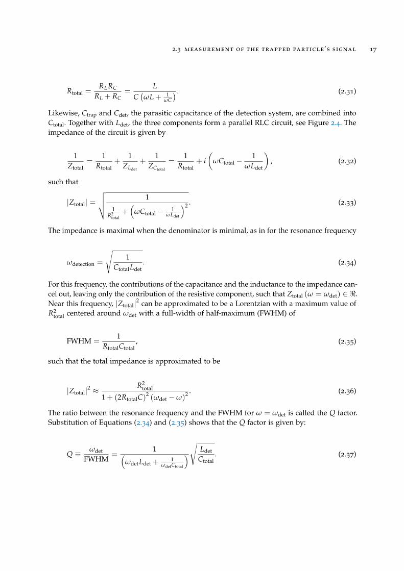
Likewise, Ctrap and Cdet, the parasitic capacitance of the detection system, are combined intoCtotal. Together with Ldet, the three components form a parallel RLC circuit, see Figure 2.4. Theimpedance of the circuit is given by

1Ztotal

=1

Rtotal+

1ZLdet

+1

ZCtotal

=1

Rtotal+ i(

ωCtotal −1

ωLdet

), (2.32)

such that

|Ztotal| =√√√√ 1

1R2

total+(

ωCtotal − 1ωLdet

)2 . (2.33)

The impedance is maximal when the denominator is minimal, as in for the resonance frequency

ωdetection =

√1

CtotalLdet. (2.34)

For this frequency, the contributions of the capacitance and the inductance to the impedance can-cel out, leaving only the contribution of the resistive component, such that Ztotal (ω = ωdet) ∈ <.Near this frequency, |Ztotal|2 can be approximated to be a Lorentzian with a maximum value ofR2

total centered around ωdet with a full-width of half-maximum (FWHM) of

FWHM =1

RtotalCtotal, (2.35)

such that the total impedance is approximated to be

|Ztotal|2 ≈R2

total

1 + (2RtotalC)2 (ωdet −ω)2 . (2.36)

The ratio between the resonance frequency and the FWHM for ω = ωdet is called the Q factor.Substitution of Equations (2.34) and (2.35) shows that the Q factor is given by:

Q ≡ ωdet

FWHM=

1(ωdetLdet +

1ωdetCtotal

)√ Ldet

Ctotal. (2.37)


The Q factor allows calculation of the time constant for dissipation of energy in the circuit:

τ ≡ Qωdet

=Ltotal(

ωdetLtotal +1

ωdetCtotal

) . (2.38)

At THe-Trap, ωz ≈ 2 · π · 4 · 106 Hz and the Q factor for ωz is measured to be around Q ≈ 800,with the time constant τ ≈ 20 ms. Both were measured by using a spectrum analyzer. It is alsopossible to measure Rtotal by measuring L using an RLC meter and then substituting Equation(2.35) in Equation (2.37). A full treatment of the circuit, as in of a series LC circuit connected inparallel to a parallel RLC circuit, instead of just a parallel RLC circuit, shows [38, 51] that at thelimit where γ FWHM the full damping term changes from Equation (2.23) to:

γ =q2ZmD2

1

1 +(

2(ω−ωdet)FWHM

)2 . (2.39)

Note that γ ∝ q2

m still holds. There is an as-of-yet unexplained discrepancy between themeasured and the calculated damping terms for hyperbolic Penning-trap experiments wherethe calculated damping term is lower by factors of between 4/5 and two than the calculated γ.In the case of THe-Trap it is about 0.7γ [36, 46, 50]. The same full treatment also shows a shiftof the resonance frequency which is negligible in the case of THe-Trap.

2.4 expansion of the electrostatic potential

For the next sections the electrostatic potential needs to be discussed in more detail. In thissection it is represented by a series expansion, with individual contributions from the differentelectrodes of the trap.The electrostatic potential for a charge-free region inside the equipotential surfaces of thePenning-trap can be described by a series expansion using Laplace’s spherical harmonicsYl,m (θ, ϕ) multiplied by rl . These terms form a complete orthogonal set which satisfy Laplace’sequation. The terms are complex, but by using specific linear combinations they can be madereal. For instance, by setting all coefficients of rlYl,m to one and taking the imaginary part ofrlYl,m in case m is positive and the real part otherwise, real terms are obtained, see Section A.2.In cartesian coordinates, these functions are homogeneous polynomials of degree l and arecalled the harmonic polynomials [52, 53, 54]. Using these harmonic polynomials the potentialcan be expressed by

φ =∞

∑l=0

(0

∑m=−l

Cl,mrl< (Yl,m) +l

∑m=0

Cl,mrl= (Yl,m)

), (2.40)

2.4 expansion of the electrostatic potential 19

where Cl,m are coefficients which can be calculated numerically or experimentally determinedas explained in Section 4.5. The total potential is the sum of contributions from the differentelectrodes, such that Cl,m → (CR,l,m + CUE,l,m + CLE,l,m), where R, UE and LE stand for ring,upper endcap and lower endcap6. Since both endcaps are grounded, their contribution iszero such that CUE,l,m = CLE,l,m = 0. For an harmonic potential of an ideal Penning-trap onlyr2Y2,0 = 2z2 − x2 − y2 contributes, such that

Cl,m =

mω2

z2q l = 2, m = 0

0 otherwise, ωz =

√2qC2,0

m. (2.41)

In reality, deviations such as the ones listed in Section 2.6 add additional terms, with the mostsignificant ones being C4,0 and C6,0

7. To make the real Penning-trap closer to the ideal oneadditional electrodes are added, called the “correction electrodes” or the “guard electrodes”.These are made to have a low r2Y2,0 contribution but a high r4Y4,0 contribution, such that byapplying a specific voltage their contribution to r4Y4,0 cancels that of the ring electrode, makingthe total r4Y4,0 component zero.The ring electrode is cylindrically symmetrical and so is the DC component of the correctionelectrodes, since the same DC voltage is applied to all of them. As a result, components withm 6= 0 or with odd l’s are negligible, such that the expression for the potential becomes

φ =∞

∑l=0

(CR,2l,0 + CCE,2l,0) r2l< (Y2l,0) , (2.42)

where CR,l,m is the coefficient of the contribution of the ring electrode to the rlYl,m term andCCE,l,mis that of the correction electrodes. One of the correction electrodes is also connectedto an AC voltage, while the other three are AC grounded. This is relevant for Section 2.5. Inorder to maintain consistency with previous theses from the group [50, 47], the coefficients areredefined using Cl ≡ CR,l,0 + CCE,l,0, such that the expression for the potential becomes

φ =∞

∑l=0

C2lr2l< (Y2l,0) . (2.43)

In this convention, C2 = V02d2 such that ωz and C2 can be written as:

ωz =

√2qC2

m, C2 =

mω2z

2q. (2.44)

6 Aside from the ring and the endcaps, there are also the skimmer electrodes, but their contribution is assumed to benegligible, both because they are grounded and because they are far away from the trap center.

7 The harmonic polynomials coupled to C4,0 and C6,0 are r4Y4,0 = 35z4 − 30z2r2 + 3r4 and r6Y6,0 = 231z6 − 315z4r2 +105z2r4 − 5r6 [52, 53, 54].


Defining VCE to be the correction electrode’s voltage used during the measurement andVCE,0

to be the correction electode’s voltage setting for which C4 = 0, C4 can be defined using thedifference between these voltages ∆VCE ≡ VCE −VCE,0 by using

C4 = ∆VCE · CCE,4,0, (2.45)

where CCE,4,0 can be found using calibration measurements, see Section 4.5, or from simula-tions CCE,4,0 = −5.34 (36) · 108m−4 [47]. The same calibration measurements show that C6 isapproximately only dependent on the ring electrode voltage, such that

C6 = V0 · CR,6,0. (2.46)

2.5 excitations and couplings

The amplitude and energies of the trapped ion’s modes can be increased and decreased usingdrive signals or swapped using coupling signals8, which is important for measuring the ion’sfrequencies and thus measuring its mass as described in Section 2.5.

2.5.1 Drive signals

Driving the Axial ModeThe axial mode can be driven by an AC signal applied to one of the endcaps at the axialfrequency. Since the upper endcap is used for ion detection, the drive signal is applied to thelower endcap. The naive approach would be to set the frequency of the axial drive signal ωAD

to that of the axial motion ωAD = ωz. However, since the axial frequency is also the resonancefrequency of the tuned circuit, applying drive signals at the axial frequency produces a signalwhich can be confused with the actual signal of the ion. It is for this reason that the ring voltageis modulated:The ring electrode’s voltage is changed from DC to a mixture of DC and AC: VR → VR +

Vmod cos (ωmod · t), where the index mod stands for modulation. If ωmod is chosen such thatωz < ωmod < FWHM, the result is that the ion’s axial mode can be excited and driven bysignals oscillating at the frequencies ω = ωz ±ωmod, also called the sideband frequencies. Thiscan be shown by observing the equation of motion for the z direction in the presence of themodulation term, a damping term and a driving term ~Edrive = Edrivez:

z = −(

ω2z +

Vmod

Vringcos (ωmod · t)

)z− γz z +

qm

Edrive. (2.47)

8 It is actually the action which is swappd during coupling. This means that the phases are changed in a predictableway. This can be relevant for phase-sensitive measurement methods such as Pulse and Phase (PnP) and Pulse andAmplify (PnA) [55].

2.5 excitations and couplings 21

Defining ε ≡ Vmod/Vring and assuming that ε 1, it can be shown [38, 36] that the expansionof the modulation contains terms of the form cos (ωdrive ±ωmod), which are resonant withthe ion’s motion when ωdrive = ωmod ± ωz, also called the sideband drive frequencies. Theupper sideband drive frequency ωmod + ωz is equivalent to a resonant drive with an amplitudemultiplier of εωz/4ωmod, but only in the limit where εωz/ωmod 1. In THe-Trap, the maximalvalues are ε = 4 · 10−4 and εωz/4ωmod = 8 · 10−3. The modulation shifts the ion’s frequencies asexplained in Section 2.6.4. The ion’s axial mode is coupled to the detection circuit and is thuscontinuously de-energized. Therefore, in order to keep the ion’s axial mode energized, thedrive signal needs to be applied continuously.

Driving the Radial ModesTo drive the radial modes a field with a large C1,1 term is required. Since the ring and theendcap electrodes have a negligible contribution to terms with odd l or non-zero m, one of thebottom correction electrodes is used instead. By applying the drive signal to just one of thefour bottom correction electrodes, a field with a relatively low symmetry is produced, suchthat it contains many terms with odd l and non-zero m, including CCE AC,1,1

9. Note that this isnot CCE,l,m, which is the coefficient of the DC voltage applied on all four correction electrodes,but the cofficient of the AC voltage applied to just one of the bottom correction electrodes.It is shown in Section A.3 that a forced harmonic oscillator has its amplitude increased byan amount proportional to the duration of the drive signal t. If the mode already has energygreater than its minimal (thermal) energy, then depending on the phase difference betweenthe drive signal and the ion motion, the energy might be at first decreased, until it reaches itsminimal (thermal) energy, at which point it will start to increase again.Unlike the axial mode, the radial modes are not coupled to the detection circuit and are thusnot de-energized “automatically”.

2.5.2 Coupling Signals

In Section A.3 it is shown that it is possible to exchange the action between two modes of motionin an oscillatory manner or increase the energy in both. This is done by applying a signal witha frequency equal to the sum or the difference of the frequencies of two modes, for instanceωcoupling = ωz ± ω±, with an electrode containing a geometric component corresponding toboth modes, for instance C2,−1 which corresponds to r2Y2,.−1 = xz or C2,1 which correspondsto r2Y2,1 = yz. Specifically, ωdrive = ω+ −ωz and ωdrive = ωz + ω− cause action exchange, alsocalled Rabi oscillations, while ωdrive = ω+ + ωz and ωdrive = ωz −ω− cause energy increasein both modes. In “sweeps”, the measurement method utilized in THe-Trap, only the former isused.Since the axial mode is continuously de-energized to its thermal limit by the detection circuit,repeatedly coupling between it and one of the radial modes can be used to de-energize thelatter to its thermal limit as well. Instead of repeatedly coupling, a “π-pulse” can be used

9 Simulations show that CCE AC,1,1/VCE AC = 1.3 m−1 [50].


as well - a coupling applied for exactly the suitable duration in order to transfer all of theexcess energy from the radial mode to the axial mode. Practically at THe-Trap, the couplingdrive is applied for about a minute while its frequency is scanned periodically across a rangeof about 100 Hz every 10 s. It was experimentally observed that for a large parameter spaceof drive amplitude, frequency scan width and frequency scan time, as long as the suitablefrequency (ωdrive = ω+ −ωz or ωdrive = ωz + ω−) is included within the scan, the radial modeis effectively de-energized to its thermal limit, as if a π-pulse was applied. This was identifiedby a previous member of the group [56] to be a classical analogy of the adiabatic rapid passage[57].

2.6 systematic shifts

The effects mentioned in Section 2.4 affect the charged particle’s frequencies of motion. As aresult the frequencies measured are “shifted”. To correct for this, the different shifts need to becalculated and then added or substracted to each measured frequency in order to arrive at thereal ones10. The shifts are divided into 4 categories: Electric field shifts, magnetic field shifts,mixed shifts, and THe-Trap shifts. In general, deviations tend to become more prominent thefurther away the ion oscillates from the trap center, as in the larger its amplitude. It is for thisreason that the energy of the modes of motion should be kept at the minimum required inorder to perform the measurement.As described in Section 4.3, in THe-Trap the trapped particle’s axial frequency is kept constantthrough a feedback loop that continuously changes the ring voltage. As a result, shifts to theaxial frequency ωz also shift the ring voltage, which then cause a shift in the radial frequenciesω±. The shifts under lock are then given by [56]

∆ω±lock = ∆ω± ±ωz∆ωz

ω+ −ω−, (2.48)

where ∆ωz is the axial frequency shift, ∆ω± are the radial frequency shifts and ∆ω±lock are theradial frequency shifts when the ion is in lock.See Section 4.11 for a list of the systematic shift values and their uncertainties for the differentions.

2.6.1 Electric Field Shifts

Since the electrodes are cylindrically-symmetric and the ion moves harmonically in the trap,many machining imperfections can be treated as cylindrically-symmetrical, such that they

10 The derivations are explained non-rigorously and the end results cited, with the exception of the relativity shift, thederivation of which can be found in Section ?? as an example for how some of the other shifts can be derivated aswell. In addition, additional formulas for the different shifts which were not used in the thesis can be found in theappendix.

2.6 systematic shifts 23

are negligible when using the invariance theorem (Equation (2.8)). In addition, the invariancetheorem holds in the case of trap tilt and trap ellipticity.

2.6.1.1 The Ctotal 4 and Ctotal 6 Shifts

The electrostatic field becomes less symmetrical due to deviations from the ideal geometryof the Penning-trap, such as machining imperfections and holes for ion injection. As a resultadditional terms Cl,m contribute to the potential. Symmetry to reflection around the z direction(Cl,m = 0 for odd l) and cylindrical symmetry (Cl,m = 0 for m 6= 0) are assumed to bemaintained. As a result, the next two largest terms after C2 are C4 and C6, as referred to inSection 2.6. It can be shown [56, 58] that the frequency shifts due to C4 are:

∆ωz

ωz=

3C4

4C2

(−2A2

+ + A2z − 2A2

−)

, (2.49)

∆ω± lock

ω±= ∓3C4

2C2

ω∓ω+ −ω−

(A2± + A2

z)

, (2.50)

and that the frequency shifts due to C6 are:

∆ωz

ωz=

45C6

48C2

(3A4

+ + A4z − 6A2

+A2z + 12A2

+A2− − 6A2

−A2z + 3A4

−

), (2.51)

∆ω± lock

ω±= ±45C6

12C2

ω∓ω+ −ω−

(A4± − A4

z + 3A2+A2− + 3A2

∓A2z

). (2.52)

Typically for THe-Trap ∆ω(12C4+)C4/ω(12C4+) ≈ 30 (30) · 10−12 and ∆ω(12C4+)C6

/ω(12C4+) ≈ 0.1 (10) ·10−12, such that both shifts are negligible.

2.6.1.2 Relativistic Shift

The relativistic mass increase of the ion changes the equations of motion and the resultingfrequencies. The derivation shows [56, 36] that substitution of the relativistic momentum~p→ γ~p = γm~v into the equations of motion while omitting non-resonance terms results in thefollowing frequency shifts:

∆ωz

ωz≈ − (ω+A+)

2 + (ω−A−)2

4c2 − 3ω2z A2

z16c2 , (2.53)

∆ω±lock

ω±≈ ∓ ω±

ω+ −ω−

(ω±A±)2 + 2 (ω∓A∓)

2 + 12 ω2

z z2

2c2 ±ω2

z

(− (ω+A+)

2+(ω−A−)2

4c2 + 3ω2z A2

z16c2

)(ω+ −ω−)ωzω±

.


(2.54)

Typically for THe-Trap ∆ω(12C4+)relativistic/ω(12C4+) ≈ −5 (10) · 10−12, such that the relativistic shiftis negligible.

2.6.1.3 Image Charge Shift

Image charges are induced in the electrodes by the trapped ion in order to keep the electrodesurfaces equipotential. As a result, an additional electric field is induced. Since the trapdimensions are significantly smaller than the wavelengths associated with the modes of motionthe field can be considered electrostatic. The induced electric field generally does not satisfyLaplace’s equation, such that the Invariance Theorem is violated and the cyclotron frequency isshifted as well. The resulting shifts are [50]

∆ωz

ωz≈ −nq

mE′z

2ω2z

, (2.55)

∆ω± lock

ω±≈ ∓

nq(

2E′ρ + Ez

)2m (ω+ −ω−)

≈ ∓n(

2E′ρ + Ez

)2B

, (2.56)

where n is the number of charges (q = ne) and E′z and E

′ρ are the axial and radial amplitudes of

the field created by the images charges, simulated for THe-Trap to be E′ρ = 4.23 (9) · 10−2Vm−2,

E′z = 8.04 (13) · 10−2Vm−2 [47].

Typically for THe-Trap ∆ω(12C4+)image charge/ω(12C4+) ≈ −310 (5) · 10−12, making the image chargeshift one of the most significant shift in terms of its magnitude, although its uncertainty isnegligible.

2.6.1.4 Trap Tilt & Trap Ellipticity

Trap Tilt:The Penning-trap is not perfectly aligned. In order to calculate the resulting shift, it is assumedthat ~B ‖ z and that the trap is tilted by θ around the y direction. Substitution of x →x cos (θ) + z sin (θ) , y→ y , z→ −x sin (θ) + z cos (θ) into the electric potential while omittingnon-resonsant terms shows that the frequencies are shifted by [50]:

∆ωz

ωz≈ −3θ2

4,

∆ω+ lock

ω+≈ 0,

∆ω− lock

ω−≈ 9

4θ2. (2.57)

Typically θ ≈ 0.1 [55] or 0.05 < θ < 0.5 [50] which lead to ∆ωzωz≈ 10 mHz and ∆ω− lock

ω−≈

20 mHz, making trap tilt and ellipticity the most dominant systematic shifts in Penning-traps


[59]. However, in practice they are cancelled out when calculating ωc using the first equationin Equation (2.8), such that they are considered negligible. The shift due to the trap tilt is notcancelled out when calculating ωc using the second equation in Equation (2.8), such that thedifference in ωc obtained with the two formulas can be used to calculate θ using [36, 38]

sin θ ≈ θ ≈ 23

√2ω+ω−

ω2z− 1, (2.58)

where ωz and ω± in the above formula are the shifted frequencies.

Trap ellipticity:The electrical shift is shifted due to elliptical deformations in the following way [36]:

~E→ ~E− mω2z ε

2q

−x

y

0

, (2.59)

where ε characterizes the strength of the elliptical deformation. The frequency shifts can beshown to be [36]

∆ω− lock

ω−=

∆ω−ω−

= −ε

2,

∆ω+ lock

ω+=

∆ω+

ω+=

∆ωz

ωz= 0. (2.60)

As mentioned above, the shift due to the trap ellipticity, just like the shift due to the trap tilt, iscancelled out to first order when calculating ωc using Equation (2.8).

2.6.2 Magnetic Field Shift - B2

Similarly to the expansion of the electrostatic potential shown in Section 2.4, the magneticpotential can be defined and expanded as well. The magnetic field is created by superconductingcoils surrounding the traps such that the trap region is source-free. As a result, the magneticfield can be defined by a scalar magnetic potential Ψ such that ~B = −~∇Ψ and ∆Ψ = 0. Similarlyto the electrostatic field, due to the rotational symmetry the coefficients of all rlYl,m with m 6= 0are zero, such that the magnetic potential can be defined by

Ψ =∞

∑l=0

B2lr2l< (Y2l,0) , (2.61)

where B2l are the coefficients of the r2l< (Y2l,0) functions and B0 = B is the magnetic fieldamplitude. The next leading order coefficient is B2. It can be shown [36, 56, 60, 58] that thefrequency shifts resulting from B2 are


∆ωz

ωz=

B2

2B0

ωc

ω2z

(ω+A2

+ + ω−A2−)

, (2.62)

∆ω± lock

ω±= ± B2

2B0

ωc

ω± (ω+ −ω−)

(ω±A2

z −ω±A2±)

. (2.63)

Typically for THe-Trap ∆ω(12C4+)B2/ω(12C4+) ≈ −20 (10) · 10−12, such that the B2 shift is negligi-

ble.

2.6.3 Mixed Shift - C1B1

Although C1 and B1 were individually treated as negligible in sections 2.6.1.1 and 2.6.2 respec-tively, their combined effect is significant due to its high uncertainty. A potential differencebetween the end-caps, for instance due to distributions of surface charges frozen on theend-caps due to the liquid hydrogen cooling, shifts the position of the ion by [50]

∆z = − qC1

mω2z

. (2.64)

In the presence of a B1 6= 0, the magnetic field changes by ∆B = B1∆z across a distance ∆z,such that the cyclotron frequency is shifted by

∆ωc

ωc=

q∆Bmωc

=q∆zB1

mωc. (2.65)

The value used for C1 in THe-Trap is C1 = 0± 1005

mVmm , with the uncertainty estimated using the

maximal drop voltage used in THe-Trap, see Section 4.1. The value used for B1 in THe-Trap isB1 = 10−3 ± 10−4 T

m based on upper limit estimations [61].Typically for THe-Trap ∆ω(12C4+)C1B1

/ω(12C4+) ≈ 0 (200) · 10−12, such that although the magnitudeof the shift is zero, it is still significant since it has the largest uncertainty.

2.6.4 THe-Trap Shifts

THe-Trap shifts are systematic shifts specific to the measurement scheme used in THe-Trap.The phase, ring modulationa and DC offset systematic shifts are a result of the ion’s axialfrequency being locked as explained in Section 3.4.1.

2.6.4.1 “Sweeps” Fit

A systematic uncertainty of either 2 mHz or 10 mHz was added to each measurement as aresult of the measurement method used in this thesis (see Section 4.8). These correspond to∆ω(12C4+)fit/ω(12C4+) = 0 (68) · 10−12 and ∆ω(12C4+)fit/ω(12C4+) = 0 (341) · 10−12 respectively, thelatter being one of the largest systematic shifts in terms of its uncertainty.


2.6.4.2 Phase Shift

A phase shift causes the error signal waveform to change its shape, shifting the equilibriumpoint of the voltage and thus the axial frequency. The shifts are

∆ωz

ωz= − γ

2ωz(∆θ)2 ,

∆ω±lock

ω±= ∓ ωz

ω± (ω+ −ω−)

γ

2(∆θ)2 . (2.66)

Typically for THe-Trap ∆ω(12C4+)phase shift/ω(12C4+) ≈ 0 (150) · 10−12, such that the phase shift issignificant due to its uncertainty.

2.6.4.3 Ring Electrode Modulation Shift

As explained in Section 2.5.1, the ring electrode’s voltage is changed from DC to a mixtureof DC and AC: VR → VR + Vmod cos (ωmod · t), where Vmod VR and ωmod ωz. Sinceωz ∝

√VR as shown in Equation (2.14), and the temporal average of the signal amplitude is not

zero due to the non-linearity of the waveform, the axial frequency is shifted by the modulationsignal. The shift can be shown to be [36, 56]

∆ωz

ωz= − 1

16

(Vmod

VR

)2

,∆ω± lock

ω±= ∓ ω2

z16ω± (ω+ −ω−)

(Vmod

VR

)2

. (2.67)

Typically for THe-Trap ∆ω(12C4+)mod/ω(12C4+) ≈ −320 (20) · 10−12, such that the modulation shiftis one of the largest shifts in terms of its magnitude.

2.6.4.4 Lock DC Offset

A DC offset to the correction voltage of the axial lock causes the error signal waveform to shiftalong the vertical direction such that the equilibrium point of the voltage shifts, which thenshifts the axial frequency. The shifts are

∆ωz

ωz= − γ

2ωz

(Voffset

Verror

)2

,∆ω±lock

ω±= ∓ ω2

zω± (ω+ −ω−)

γ

2ωz

(Voffset

Verror

)2

, (2.68)

where γ is the damping defined in Equation (2.23).Typically for THe-Trap ∆ω(12C4+)DC offset/ω(12C4+) ≈ −1 (0.1) · 10−12, such that the DC offset isnegligible.

2.6.4.5 Coil Pushing

The tuned circuit has been observed to “jump” every few hours, such that the tuned circuitis shifted by about −300 Hz and then returns to the previous value after about one hour. Thecause is assumed to be the amplifier heating the liquid helium around it, occasionally creating


bubbles which might get trapped for a while and change the resonance frequency by changingthe capacitance. A relative uncertainty of ∆ω(12C4+)coil pushing/ω(12C4+) ≈ 0 (40) · 10−12 was assignedin order to account for this [61].

3T H E E X P E R I M E N TA L S E T U P

THe-Trap, originally UW-PTMS, is a Penning-trap experiment utilizing a ~5.2 Tesla super-conducting magnet (see Section 3.1) built in 1998 and originally located at the University ofWashington, Seattle, under the supervision of Prof. R. S. Van Dyck Jr. [62]. In 2008 it was movedto the Max Plank Institute for Nuclear Physics in Heidelberg, Germany, under the supervisionof Prof. Klaus Blaum [48]. The experiment spans across two rooms. The upper room containselectronics and cabling and a crane for controlling and lifting the experimental apparatus (seeSection 3.2). The lower room contains the superconducting magnet, the experimental apparatuspositioned inside the magnet, the stable power supply and the environmental stabilizationsystem (see Section 3.3).In Section 3.1 the superconducting magnet is described as shown in Figure 3.1 including itsrepair (Section 3.1.1), shimming as shown in Figure 3.3 (Section 3.1.2) and shielding factormeasurements as shown in Figure 3.4 (Section 3.1.3). In Section 3.2 the experimental apparatusis explained including the gas inlet system as shown in Figure 3.6 (Section 3.2.1). In Section 3.3the stabilization system is expanded upon including the new data acquisition system (Section3.3.1) and website (Section 3.3.2). In Section 3.4 loading and manipulation of ions is discussedincluding locking and detecting the axial mode as shown in Figure 3.11 (Section 3.4.1) anddetection of the radial modes (Section 3.4.2).Additional details on the experimental setup are found in the following theses [62, 63, 58, 47,50] and articles [48, 64].

3.1 the magnet

The ~5.2 Tesla superconducting magnet was designed by Prof. R. S. Van Dyck Jr. [65] andbuilt by Nalorac Cryogenic Corporation in 1998. Its internal structure is onion-like in order tominimize Liquid Helium (LHe) losses. Specifically, the superconducting coils are submerged inLHe, which is enclosed in a vacuum layer, a Liquid Nitrogen (LN) reservoir and a layer of thesame vacuum. There are three LHe ports - the cold bore where the trap tower is inserted into,the “charging stack” which is used for charging the magnet and the “filling stack” which isused for filling LHe. There are two LN2 ports or “stacks” for filling LN2. See Figure 3.1.The largest contribution to the measurement uncertainty comes from temporal fluctuationsin the magnetic field. As a result there are several mechanisms in place to keep the magneticfield static. To damp vibrations, the LHe reservoir, including the superconducting coils holdercalled the “pot”, are suspended on the bore joint from above, see Section 3.1.1. In addition,the magnet is placed on foundations which are mechanically de-coupled from those of thebuilding. To reduce temperature fluctuations, which cause permeability and thus magnetic

29

30 the experimental setup

Figure 3.1: The magnet as described in Section 3.1. The superconducting coils are held in a structurecalled the “pot” submerged in LHe. A level sensor is used as part of a system for regulatingthe LHe pressure and level. Surrounding the LHe reservoir are insulation compartments forreducing LHe loss - a vacuum compartment, a liquid nitrogen reservoir with two openingsfor filling and another vacuum compartment. The LHe reservoir has three openings: The“bore” is used for inserting the experimental apparatus and the left and right “stacks” areused for charging and filling the magnet respectively. Note that the LHe reservoir is hungfrom above through flexible bellows on the stacks and the bore joint on the bore in order tosuppress vibrations and so magnetic field fluctuations.

3.1 the magnet 31

Figure 3.2: The magnet’s relative magnetic field decay rate in ppt/h(

10−12/h). Starting at hundreds of

ppt/h in Seattle, it went down to 1 ppt by 2007. In 2009 the magnet was moved to Heidelbergand recharged, reaching the same order of magnitude after about seven years. At the end of2015 the magnet was charged again, this time using the trick of overcharging the main coilcurrents to 100.2% of the desired current and then lowering it back to 100%. It is probably asa result of the overcharging trick that the decay rate decreased faster, achieving the sameorder of magnitude as in Seattle within four years.

field fluctuations, the helium gas pressure and LHe level are regulated with the use of pressureand level sensors controlling valves and a pump, see Section 3.3. Temperature fluctuations arefurther suppressed by the bore being a cold bore, which results in the experimental apparatusbeing kept at a constant LHe temperature. To suppress external magnetic field fluctuationsadditional superconducting coils are used, called shielding coils, which have a similar structureto that of the main coils and passively suppress changes to the magnetic field by inducedcurrents, see Section 3.1.3. Magnetic field fluctuations are monitored using a fluxgate sensor,which can be connected to Helmholz coils surrounding the magnet to suppress the magneticfied fluctuations in the lower trap region by a factor of three [50]. The Helmholz coils were notused in this thesis. Lastly, shimming coils are used to make the magnetic field homogeneous inthe trap region. These are superconducting coils arranged in different configurations such thateach has a strong contribution to the magnet field with respect to a specific spatial component,for instance x or y2. They can be tuned to cancel out the spatial components of the maincoils, see Section 3.1.2. The resulting temporal decay rate of the magnetic field due to theabove-mentioned suppression mechanisms is considered especially low in comparison to othermagnets, see Figure 3.2.


3.1.1 The Repair of the Magnet

The magnet quenched in January 2015 due to miscommunication regarding the filling of liquidnitrogen (LN). Following the quench, the vaccuum of the magnet was tested under both roomtemperature conditions and LN temperature several times. The temperature changes due to thetests led to a leak and eventually to a complete break of the glue in the bore joint, which is ajoint connecting the two G10 parts of the bore with the epoxy glue Armstrong A12, see Figure3.1. As the glue broke, the LHe reservoir, including the chamber containing the superconductingcoils called the “pot”, dropped a few centimeters onto the 20 K surface shield, stretching theflexible bellows of the LHe stacks. In addition to the repair of the joint it was decided tohave the magnet undergo a maintenance phase, both of which were performed by the groupmembers. During the maintenance phase part of the magnet top cover and many O-Rings werefound to be in an eroded state and were replaced with new Viton ones. To prevent erosion,epoxy spray was sprayed on the magnet top cover, its screws were sealed with theorstat andtape and the stacks were surrounded by Styrofoam and towels. The O-Rings beneath the LN2

stacks were not replaced as it was impossible to do so without cutting the magnet open. Inaddition, “Spring-loaded studs” were used to seal the magnet’s bottom entrance port to beused as an extra emergency exit path for LHe in case of a quench. In October 2015 the repairwas finished, the magnet charged and shimmed and the trap tower re-inserted.

3.1.2 Shimming the Magnet

Shimming is the process of making the magnetic field more homogeneous around a specificregion, in this case the region of the lower trap. It is done by the use of the shimming coils,which are coils arranged such that each primarily contributes to a specific spatial componentof the magnetic field, such as x, y or z2. By applying the suitable amount of current to eachcoil the non-homogeneus contributions of the main and the shimming coils cancel each otherout. In 2009 the magnet was not shimmed as the electrical connections were blocked withice. The relative homogeneity of the magnet was ≈ 10−5 around a 1 cm3 volume [66]. Afterthe magnet repair in 2015 the opportunity was used to shim it to a relative homogeneity of8.2 · 10−8 around a 1 cm3 volume, see Figure 3.3, which is about 100 times more homogeneousthan before. The measurement was performed using an NMR probe inserted into a “warmbore”, a cylinder-shaped structure capped from the bottom inserted into the bore in order tomake the bore region temporarily LHe-free and warm enough for shimming. Initially a watersample was used, but due to the below-freezing temperature inside the warm bore it wasreplaced with an acetone sample.

3.1 the magnet 33

Figure 3.3: The results of shimming the magnet - the magnetic field in µT as a function the axial distancefrom the trap center in cm. The homogeneity, or relative uncertainty of the magnetic field atthe trap region, which corresponds to the position z = 0, is shown to be 8.2 · 10−8.

3.1.3 Shielding Factor Measurements

In addition to the main superconducting coils for generating the magnetic field and theshimming superconducting coils, there are additional superconducting coils for suppressingmagnetic field fluctuations, for instance due to movement of people or objects in the vicinity ofthe magnet. The reciprocal of the suppression ratio in the trap region, or the ratio between themagnetic field measured outside of the magnet and the resulting magnetic field in the trapregion is called the shielding factor. The shielding factor was measured to be 180 (uncertaintyunknown) back when the magnet was in Seattle [65]. Since then, three additional measurementswere performed in Heidelberg, see Figure 3.4. All three measurements use external Helmholzcoils for changing the magnetic field in the trap region. The first measurement yielded 169(13)and was performed using a Fluxgate Magnetometer before the magnet was charged followingthe quench in 2015. The second measurement resulted in 179(14) and was performed usingan NMR probe after the magnet was recharged. The third measurement yielded 173(2) andwas performed after inserting the experimental apparatus (Section 3.2) back into the magnetand successfully loading and manipulating 12C4+ ions. It involved repeatedly measuring themodified cyclotron frequency of a 12C4+ ion using the “sweeps” measurement method (seeSection 4.8) while changing the magnetic field in the trap region. The changes in the cyclotronfrequency correspond to changes in the magnetic field in the trap region by the use of Equation(2.2).


3.2 the trap tower

The Penning-trap is connected to a tower-shaped structure which is inserted into the super-conducting magnet, see Figure 3.5. At the top is a scroll pump (not drawn), a turbo pump,an ion source which was never used, the gas injection system (not drawn, see Section 3.2.1)and outlets for electrical connections going down into the traps region. Near the bottom ofthe tower are two hyperbolical Penning-traps, only the bottom of which is in use. Below itat the very bottom is the resonator, the cryo-amplification and a field emission point (FEP),see Section 3.4. The traps are separated from the rest of the trap tower by a manual valve andby a computer-controlled pneumatic valve [47], which automatically closes when the vacuumpressure exceeds a certain threshold (not drawn).

3.2.1 The Gas Inlet System

A gas inlet system was implemented, allowing trapping of ions not available by extractionfrom the trap surfaces or from the residual gas, see Figure 3.6. A gas bottle containing either anatural mixture of neon isotopes or a mixture enriched in 22Ne is connected to the apparatusthrough a pressure reducer and a series of valves. A fine-leak valve is used to introduce theminimal neon pressure necessary for loading neon ions. For the neon loading process, all othervalves between the neon gas bottle and the traps are open except for a computer-controlledpneumatic valve. This valve is opened for a duration of one second during ion loading, seeSection 3.4. This introduces neon gas into the trap region which is then ionized using the FEP(see Section 3.4) and trapped. The pressure in the trap region is low enough such that ions canstay trapped for several weeks.

3.3 the stabilization system

As mentioned in Section 3.1, temporal and spatial magnetic field stability is important andachieved primarily by stabilization of the helium gas pressure and LHe level, see Figure 3.7. Thepressure in the bore is continuously compared and regulated to that of an Absolute PressureReference (APR) by the use of a valve and a pump. The level in the bore is continuouslycompared and regulated to a reading from a level sensor unit with the use of two valves, onecontrolling pressure release from the bore and the other from the reservoir. Aside from thepressure and the level, the temperature in both rooms is regulated as well. Other parameters,such as the pressure in the room itself, the temperature in different positions in the room, thehumidity and changes in the magnetic field are also recorded [67].

3.3 the stabilization system 35

(a)

(b)

(c)

Figure 3.4: Shielding factor measurements. Graph (a) was measured before the magnet was rechargedand displays the shielding factor as the ratio between the magnetic field measured insidethe magnet using a fluxgate magnetometer and that applied externally using Helmholzcoils surrounding the magnet. The height scale is shifted such that the origin correspondsto the location of the bottom trap. Graph (b) was measured after the magnetic field wascharged and displays the same but using an NMR probe. The height scale has a differentorigin than in (a) but is shifted such that the origin corresponds to the location of the bottomtrap. Graph 3 was measured after the experimental apparatus (Section 3.2) was re-insertedand ion loading and manipulation was re-established. It displays the magnetic field changecorresponding to changes in the cyclotron frequency of a 12C4+ as a function of that of theHelmholz coils. All three measurements are in agreement. See Section 3.1.3.


Figure 3.5: The trap tower and the two traps. For more details see Section 1.1.

3.3 the stabilization system 37

Figure 3.6: The gas inlet system. A neon gas bottle is used to inject gas down into the Penning-traps region containing the storage trap and the experimental trap beneath it. The gas isinjected through a pressure reducer, a fine-leak valve, a manual valve, a computer-controlledpneumatic valve and a bakeable manual valve. For injecting neon these are all kept openexcept for the pneumatic valve, which is opened for one second during electron emission,see Section 3.4. Regarding the other components - manual valve 2 is the only manual valvewhich stays closed in regular operation as it is used for pumping the system following gasbottle exchange. The emergency valve closes automatically in case the pumps fail and therough pressure exceeds 0.1 mbar. The ion storage trap was never used.


3.3.1 New Data Acquisition Program - “PyEnvDAQ”

The system parameters were originally recorded using a program written in C . A new programwas written in Python, “PyEnvDAQ” (Python Environmental Data Acquisition System), seeFigure 3.8. The new program provides additional features such as email and Telegram alerts incase the values of recorded parameters are found outside of their pre-defined ranges, advancedplotting options and export options. It also outputs the recorded data in a new format which iscompatible with the new controller [68].

3.3.2 New Group Website - “THe-Website”

The group website was redesigned in order to provide compatibility with the new massmeasurement data file formats created by the new controller program [68] and with the newstabilization system data format created by PyEnvDAQ, see Section 3.3.1. It also provides moreplotting options for the parameters of the stabilization system, an updated links menu and pre-analysis of calibration data in real time, helping with decision-making during measurementsand thus speeding up the process.

3.4 loading and manipulating ions

Ions are loaded using a Field Emission Point (FEP) which releases an electron beam of a fewnA. These electrons then oscillate between the FEP and the top skimmer electrode, which isan electrode placed between the two traps, until they collide either with residual or injectedgas molecules, for instance injected neon gas, or with the trap surfaces, releasing and ionizingatoms absorbed into the trap surfaces in the process. The ions are trapped using the electrostaticand the magnetic fields of the trap. In THe-Trap a FEP voltage of −230V is required to ionize12C4+ from the trap surfaces and −390V for ionizing 20Ne8+ and 22Ne7+ from injected neon gas.The process for removing ions until only one is left is described in Section 4.1. The detectableand trappable ions in THe-Trap are shown in Figure 3.10 and [48, 63].

3.4.1 Locking and detecting the Axial Mode

The axial frequency is kept constant, or locked. This cancels axial frequency shifts caused byenergy changes of the radial modes and is essential for the measurement process, see Chapter 4.The locking is achieved by the use of a correction circuit, see Figure 3.11. The ion’s axial mode

3.4 loading and manipulating ions 39

Figure 3.7: The stabilization system. The helium gas pressure in the bore is continuously compared andregulated to that of an Absolute Pressure Reference (APR) unit using a PI control system (notdrawn) which controls both the bore and the pump automatic valves. The liquid helium levelis measured and regulated using a PI control system which controls the reservoir automaticvalve and thus the helium gas pressure in the reservoir. The bore, reservoir and pump bypassvalves are closed during regular operation, such that the helium gas from the bore and thereservoir flows through their respective automatic valves through the pump and its valvesto the outside. In this way both the helium gas pressure and the liquid helium level in thebore stay constant. It is also possible to turn off the level stabilization system by openingthe bore and reservoir bypass valves, such that the helium gas flows from the bore and thereservoir through the pump and its valves straight to the outside. The pump and its valvesare bypassed during liquid helium filling by opening the pump bypass valve. For a moredetailed drawing and explanation see [67].


Figure 3.8: The new data acquisition program - “PyEnvDAQ” as described in Section 3.3.1. The programhas 3 tabs, or windows. The channels tab displays 25 channels of recorded data including theraw data, its physical unit, calibration factors and the calibrated values. It is also possible toset minimal and maximal ranges for each parameter such that an alarm is sent per email andper Telegram when the measured value gets out of range. The actions tab allows plottingand exporting of the recorded channels. The messages tab shows timestamped alerts forparameters that are outisde of their specificed ranges.


Figure 3.9: The new group website, “THe-Website”, as described in Section 3.3.2. “Plot EnvironmentalData” allows plotting of up to 2 environmental channels simultaneously such as pressure,temperature and magnetic flux. “Plot Flow Data” plots the helium and nitrogen gas flows.“Overview” plots a set of pre-configured plots of important recorded parameters such that theuser can get a quick glimpse of the state of the system. The rest are links to other websites.


(a)

(b)

Figure 3.10: A ring voltage scan revealing trappable ion species in THe-Trap: 1H+ and 2H+ ,4He+ to4He2+ ,12C2+ to 12C4+ ,14N3+ to 14N5+ ,16O3+ to 16O6+ ,19F4+ to 19F7+ ,20Ne4+ to 20Ne8+,22Ne4+ to 22Ne8+,35Cl6+, 35Cl7+ and 45Sc9+. To plot the graphs, ions were loaded and thering voltage was sweeped while observing the amplitude of the signal coming from thetrap. As the ring voltage changes, so does the axial frequency of the ions. When the axialfrequency of an ion equals that of the detection circuit, the ion releases its energy in theform of a visible peak. The peaks can be identified with specific ion species using Equation(2.14) and extrapolation from known values such as 91.144V for 12C4+. Note that the stablevoltage source can only be set between −100V and 0, such that a different voltage sourcewas used to explore the −170V to −100V region. This voltage source can be used to trapthe ions but is not stable enough in order to perform precision mass measurements.


is continuously excited using a ≈ 4.1 MHz signal (see Section 2.5.1), producing a constant≈ 4 MHz ion signal which is detected using the detection circuit, see Section 2.3. The same≈ 4.1 MHz excitation signal is also mixed with the ≈ 4 MHz ion signal such that signals at≈ 100 kHz and ≈ 8.1 MHz are produced. These are filtered by a 100 kHz band-pass filter suchthat only the ≈ 100 kHz component is left. It then gets mixed with another 100 kHz signal,called the mixing signal, to produce signals at ≈ 200 kHz and at DC. These are filtered by alow-pass filter such that only the DC component is left. Setting the phase of the 100 kHz mixingsignal properly causes the DC signal to have a dispersion shape with respect to changes inthe axial frequency. This DC signal, called the error signal, is integrated, divided and thenconnected as the ground or “low” of the ring electrode voltage, the “high” being a sum of afixed DC contribution and the ring modulation signal1. This creates a feedback loop whichkeeps the axial frequency constant.Initially, the mixing down of the 100 kHz signal to DC and its integration were performed by acustom-made box called the “mix2dc box”2. After performing the first 20Ne8+ measurementthe box broke and was replaced with a commercial Zurich Instruments “HF2LI” Lock-InAmplifier, see Figure 3.11. The Lock-In Amplifier mixes the ion signal from 4 MHz straight toDC with no 4.1 MHz or 100 kHz mixing in-between and uses the resulting DC signal as theinput for a feedback (PID) circuit. The rest of the circuit remains the same. Unlike the analogmix2dc box, the Lock-In Amplifier is digital. This means its phase is arbitrarily reset wheneverone of its parameters is adjusted, such as the mixing frequency, which means that the phasehas to be calibrated more often than for the mix2dc box, see Section 4.3.

3.4.2 Detecting the Radial Modes

Unlike the axial mode, which interacts with the detection circuit and leaves a recognizablepeak, the radial modes cannot be directly detected. Rather, they are detected indirectly througha change in the axial frequency, or under axial lock a change in the lock error signal. Effectssuch as relativity, C4 6= 0 and B2 6= 0 cause the frequency of each mode to be dependent on theenergy of all three modes. Specifically, the axial frequency is dependent on the energy of themodified cyclotron and the magnetron frequencies. Using Equations (2.49) , (2.62) and (2.62), itis obtained that the relative axial frequency shift up to second order in A2

± is given by

∆ωz

ωz=

(−3C4

2C2+

B2

2B0

ωc

ω2z

ω+ −ω2+

4c2

)A2+ +

(−3C4

2C2+

B2

2B0

ωc

ω2z

ω− −ω2−

4c2

)A2−. (3.1)

1 The ring voltage is negative, such that the “high” is actually at most +100 µV and the “low” is negative tens ofvolts, for instance −90 V for 12C4+.

2 The mixing of the DC and AC components of the ring voltage is done by another custom-made box called the“wing box”, omitted from the drawing, which applies another low-pass filter on the DC component and is capableof switching the “high” of the ring voltage between two voltage sources. At one point during the measurements itbroke and a replacement with a similar functionality was internally constructed.


(a)

(b)

Figure 3.11: (a) The old axial locking circuit with the “mix2dc box”. The ion signal is mixed down from4 MHz to 100 kHz and then to DC. It is then integrated, divided and set as the ground or“low” of the ring voltage, the “high” being a sum of a fixed DC contribution and the ringmodulation signal. This creates a feedback loop which keeps the ring voltage, and so theaxial frequency, constant. (b) the new axial locking circuit with the Lock-In Amplifier. Theion signal is mixed down from 4 MHz directly to DC, is amplified, integrated and derivated(PID) as opposed to just integrated, and the attenuation and division factors are different,but effectively the functionality is the same as for (a). See Section 3.4.1 for more details.


Under lock, it is not the axial frequency which is shifted, but the lock error signal. The mea-surement method for detecting ω± involves radially exciting the ion with varying frequenciesωguess − ∆ω

2 < ω < ωguess +∆ω2 via one of the correction electrodes while observing the lock

error signal, where ωguess is a guess value for ω± and ∆ω is the scan width. If the real ω± isfound inside the scan range, at some point the excitation frequency will be equal to ω± and theω± mode will be energized, causing the axial frequency to shift since to lowest order ∆ωz

ωz∝ E±

, or rather the lock error signal will shift since the axial frequency is locked. The frequency forwhich the lock error signal shifts is ω±. See Section 4.8 for more details.

4N E O N M A S S M E A S U R E M E N T S

In this chapter the neon mass measurements performed in the context of this thesis aredescribed. In Section ?? the measurement process is elaborated upon. Specifically, in Section 4.1it is explained how a single ion is loaded into the trap. In Section 4.2 it is shown how pulsesexciting the radial modes were used to roughly measure the ion frequencies. In Section 4.3the process of locking the ion is elaborated upon. In Section 4.4 it is shown how to align thetrap. In Section 4.5 the different calibration measurements are explained. In Section 4.8 themeasurement method for precisely finding the ion frequencies is shown. In Section 4.9 thecalculation of the systematic shifts is explained. In Section 4.10 the data analysis is described. InSection 4.11 the measurement results are shown. Specifically, Sections 4.11.1 and 4.11.2 containthe measurement results for 20Ne8+ and 22Ne7+, respectively.

4.1 loading a single ion

To prepare a single ion, first many ions are loaded using a FEP voltage of −230 V for 12C4+

or −390 V for 20Ne8+ and 22Ne7+ as explained in Section 3.4. Next, high amplitude (5 Vpp)excitation signals called “brooms” are applied to the lower endcap with frequencies rangingfrom around twice the magnetron frequency of the ion of interest (several hundred kHz) toabout twice the axial frequency of the ion of interest (several MHz), except for a windowseveral tens of kHz wide around the axial frequency of the ion of interest. In this way the axialmodes of all ions in the trap except for that of the ion of interest are energized. This causesall ions other than the ion of interest to oscillate at high amplitudes. As a result some collidewith the endcaps and exit the trap. The brooms are followed by a reduction in the ring andring correction voltages (in absolute value) called a “drop” which lasts 10 s. During a drop,the potential well is temporarily shallow, causing energetic ions to exit the trap. Once the ringvoltage is restored to its original value, magnetron coupling is performed to de-energize themagnetron mode of the ion of interest, which is excited by the brooms via the fz − f− sidebandas explained in Section 2.5.2. The axial mode of the ion of interest is then energized with apulse as explained in Section 2.5.2. The resulting signal picked up by the amplifier showsseveral peaks in case there are many ions left or a single peak in case there are few ions or asingle ion left. The sequence of brooms, drop, magnetron coupling and axial excitation arerepeated with the drop voltages decreasing (in absolute value) from a few negative volts to afew negative tens of mV until the axial excitations show a single peak. There are then severalways to verify whether there is a single ion left in the trap:An “Ion dip measurement” can be performed by continuously exciting the axial mode asexplained in Section 2.5.2 while recording and averaging the resulting ion signal. The existence

47

48 neon mass measurements

of additional ions can be verified or excluded by measuring the damping term, which is thewidth of the resulting dip, see Section 2.3.4. Alternatively, the stability of the axial lock can beobserved. When several ions are present in the trap, they apply forces on each other, causingenergy exchange between one another. Abrupt shifts in the error signal are observed as aresult. In addition, the “ring/correction ratio”, also called the “trap orthogonality constant”or the “tuning ratio” can be measured. In the case of THe-Trap, a change in the ring voltageof 1 mV requires a change of 750 mV in the correction electrodes voltage in order to keep theerror signal constant. In the presence of several ions the potential seen by the ion of interestchanges and as a result the ∆Vcorr/∆Vring ratio changes by about a factor of 1/2. However, evenif all tests are consistent with having a single ion, it is still possible that there are additionalones with radii and energies so large that they do not affect the ion of interest. Such ions mightde-energize over days or weeks and then become detectable.Loading the trap creates “patch potentials” which are charges trapped on the surfaces of thetrap. Patch potentials shift the minimal drop voltage required to get a single ion, the calibrationparameters (see Section 4.5) and the “magic ring correction voltage” (see Section 4.8), such thatthe calibration measurements need to be manually repeated between loadings. This is the mainsource of systematic uncertainty in the measurement as explained in Section 4.11.

4.2 pulsing the radial modes to roughly determine the ion frequencies

In Section 4.1 the trap voltages were adjusted to determine the axial frequency to within2 Hz. Next, a rough value for the magnetron frequency is found using magnetron excitationpulses. A magnetron pulse is applied, typically at an amplitude of 5 V and a duration of10 ms. Then, coupling is performed as explained in Section 2.5.2. If an ion signal is observed, itcan be concluded that the magnetron pulse successfully energized the magnetron mode. Thecycle of magnetron pulse and magnetron coupling is then repeated while gradually changingthe magnetron pulse frequency, lowering its amplitude to around 100 mV and increasing itsduration to around 1 s. In this way the magnetron frequency is determined to within 1 Hz.Next the modified cyclotron frequency is found using the same method with cyclotron pulsesand cyclotron coupling using a starting value calculated using Equation (2.10).

4.3 lock phase calibration and locking the ion

Once there is a single ion in the trap, the axial frequency has been set to be the resonancefrequency of the tuned circuit within 2 Hz and the magnetron mode has been de-energized,locking is established as explained in Section 3.4.1. First the phases of the lock-related signalsare calibrated by fixing the mix2dc or LIA error signal and measuring the resulting ion signal asa function of the phases of the lock-related signals, see Figure 4.1. In the case of the mix2dc box,these are the two 100 kHz mixing signals and the 4.1 MHz excitation signal. In the case of theLIA, these are the LIA 4 MHz mixing signal and the 4.1 MHz excitation signal. A second-degreepolynomial fit is applied to find the phases for which the ion signal amplitude is maximal.

4.4 aligning the trap 49

(a)

Figure 4.1: Lock Phase Calibration Measurements. The ion signal amplitude is maximized by tuning thephases of the lock-related signals as explained in Section 4.3.

Once the phases have been calibrated, the error signal is set to be no longer fixed, and in thecase of the LIA the PID feedback parameters are then automatically tuned by the LIA’s controlprogram. At this point the ion is locked but at an arbitrary error signal value. The ring voltageis then modified in steps of 1 µV until the error signal is zero, which means that the axialfrequency has been determined to within the noise of the detection circuit and the voltagesource, which is a few µV or a few 100 mHz.

4.4 aligning the trap

Once axial locking has been established the trap can be aligned to be perpendicular to ~B. Theprocess of alignment involves tilting the trap in steps using an xy displacement and tiltingstage connected to the trap tower (see Section 3.2) and observing the resulting axial frequency,which is maximal when the trap is aligned. Initially the steps cause large changes in the axialfrequency such that it is roughly measured using axial excitation pulses. The final steps causesmaller changes which can be measured while the ion is locked for fine tuning. The trap canbe aligned with a precision of about δθ = 0.1 using this method. In practice, the trap tilt isnegligible due to the use of the invariance theorem, see Equation (2.8), for the determination offc [36].


4.5 radial and axial calibration measurements

Once the phases of the lock-related signals are calibrated and ion locking is achieved, radialand axial calibration measurements are performed. These calibration measurements are usedfor determining the C4, C6, B2, relativistic and sweep fit systematic shifts (see Section 2.6), seeSection 4.8. The calibration results are given in Table 4.1.

4.6 magnetron and modified cyclotron calibration measurements

In the modified cyclotron and magnetron calibration measurements, the dependency of theaxial frequency on the energy in the radial modes is measured, see Figure 4.2. The ringcorrection voltage for which the axial frequency is the least dependent on the pulse amplitudeis found, along with their scaling factor, both of which are needed to calculate the systematicshifts mentioned above. This is done by de-energizing the radial modes, locking the ion,measuring the average error signal, exciting the respective radial mode using a pulse, re-locking the ion and measuring the average error signal again1. The measured difference inerror signal corresponds to the axial frequency shift caused by the respective radial modebeing energized. The process is repeated for different pulse energies. Specifically, the pulseduration is kept constant at 50 ms for the magnetron excitation or 65 ms for the modifiedcyclotron excitation. As discussed in more detail below, the relative error signal change scaleslinearly with the square and quadrature of the pulse amplitude. As a result the measurementis fitted to y = ax2 + bx4, where x and y are the pulse amplitude and the error signal shift,respectively. The measurement is then repeated for different correction electrode voltages andlinearly fitted such that y = cx + d, where x and y are the ring correction electrode voltage andthe a parameter from the previous fit, respectively. The average b parameter, the ring correctionelectrode voltage for which a = 0 and the c parameter are used to calculate the systematicshifts mentioned above.Specifically, for the magnetron mode, the relative axial frequency shift due to a change in themagnetron amplitude up to fourth order is given by the C4 and C6 shifts (see Section 2.6.1.1)2:

∆ωz

ωz= −3C4

2C2A2− +

45C6

16C2A4−, (4.1)

The relative change in the axial frequency is expressed using a linear approximation of Equation(2.14):

1 The error signal for the de-energized state is measured multiple times in order to minimize ring voltage fluctuationeffects.

2 The relativistic and B2 shifts were neglected. For example, the absolute values of the A2− coefficients for the first

12C4+ measurement (see Section 4.11) are about 1.5, 5 · 10−2 and 8 · 10−6 for the C4, B2 and relativistic shifts,respectively.

4.6 magnetron and modified cyclotron calibration measurements 51

(a)

(b)

(c)

Figure 4.2: Magnetron and modified cyclotron calibration Measurements. (a) One of the radial modes isenergized with pulses of different amplitudes and the corresponding lock voltage shift ismeasured and fit. The measurement is repeated for different correction voltages. (b) the aparameter from each fit in (a) is linearly fit to find the correction voltage for which a = 0. (c)The b parameter from each fit is averaged to arrive at the value for b. These parameters arenecessary for calculating certain systematic shifts, see Section 4.7.


∆ωz

ωz=

∆Vring

2Vring. (4.2)

The ring voltage change ∆Vring is expressed as the lock correction voltage change divided bythe calibration factor Vlock cal (see Section 3.4.1):

∆Vring = − ∆Vlock

Vlock cal, (4.3)

such that the relative change in axial frequency is given by

∆ωz

ωz= − ∆Vlock

2VringVlock cal. (4.4)

The magnetron, axial and modified cyclotron amplitudes A+ , Az and A+ can be related to thepulse amplitudes and durations by the use of the calibration constants Acal + , Acal z and Acal +respectively:

A+/z/− = Acal +/z/-Apulsetpulse. (4.5)

Substitution of Equations (2.44) , (2.45) , (4.4) and (4.5) into Equation (4.1) yields the relationbetween the change in lock voltage and the pulse amplitude

∆Vlock = amag · A2pulset2

pulse + bmag · A4pulset4

pulse, (4.6)

where

amag ≡6q∆VCECCE,4,0VringVlock cal

mω2z

A2−cal (4.7)

and

bmag ≡ −45qC6VringVlock cal

4mω2z

A4−cal (4.8)

are determined from the fit in Figure 4.2(a). In Figure 4.2(b) amag is fit as a function of thecorrection voltage ∆VCE. The curvature cmag is given by

cmag ≡6qCCE,4,0VringVlock cal

mω2z

A2−cal, (4.9)

4.6 magnetron and modified cyclotron calibration measurements 53

and the intersection point with the horizontal axis occurs at VCE = Vmag, which is V0 fromFigure 4.2(b) and is the correction voltage for which the axial frequency is the least dependenton the magnetron energy. In Figure 4.2(c) bmag is fit, which allows A− cal and C6 to be calculatedusing

A− cal =

√cmagmω2

z

6qCCE,4,0Vlock calVring(4.10)

and

C6 = −4mω2

zbmag

45qA4−calVringVlock cal

. (4.11)

A− cal, C6 and Vmag are necessary for calculating the C4, C6 and relativistic systematic shifts.The relative axial frequency shift due to a change in the modified cyclotron amplitude is givenby

∆ωz

ωz= −3C4

2C2A2+ +

45C6

16C2A4+ +

B2

2B0

ωcω+

ω2z

A2+ −

ω2+

4c2 A2+, (4.12)

which in comparison to Equation (4.1) also includes the B2 and relativistic shifts as they arenot negligible. Substitution of Equations (2.44) , (2.45) , (4.4) and (4.5) into Equation (4.6) yieldsthe relation between the change in lock voltage and the pulse amplitude

∆Vlock = acyc · A2pulset2

pulse + bcyc · A4pulset4

pulse, (4.13)

where

acyc ≡ −2VringVlock cal

(−

3q∆VCE · CCE,4,0

mω2z

+B2ωcω+

2B0ω2z− ω2

+

4c2

)A2+cal (4.14)

and

bcyc ≡ −45qVringVlock calA4

+calC6

4mω2z

(4.15)

are determined from the fit in Figure 4.2(a). In Figure 4.2(b) acyc is linearly fit to the correctionvoltage, from which the curvature ccyc is obtained:

ccyc ≡6qVringVlock calCCE,4,0A2

+cal

mω2z

. (4.16)


The intersection point with the horizontal axis gives

B2 =Bω2

z2c2 +

6∆VCE · CCE,4,0

ω+(4.17)

and occurs at VCE = Vcyc, which is V0 from Figure 4.2(b) and is the correction voltage for whichthe axial frequency is the least dependent on the modified cyclotron energy. In Figure 4.2(c)bcyc is fit, which allows A+ cal and C6 to be calculated using

A+ cal =

√ccycmω2

z

6 · CCE,4,0qVlock calVring(4.18)

and C6 = −4mω2

zbcyc

A4+cal45qVringVlock cal

, (4.19)

which together with B2 and Vcyc are necessary for calculating the C4, C6, relativistic and B2

systematic frequency shifts (see Section 2.6).

4.7 axial calibration measurements

In the axial calibration measurement, the dependency of the axial frequency on the energy inthe axial mode is determined, see Figure 4.3. Unlike for the radial modes, pulses cannot be usedas the axial mode is continuously excited by the 4.1 MHz excitation signal and de-energizedby the tuned circuit. Thus, the error signal shift is measured as a function of the amplitudeof the 4.1 MHz excitation signal. This is done by measuring the average error signal as afunction of the the 4.1 MHz excitation signal amplitude. The measured difference in errorsignal corresponds to the axial frequency shift caused by the energy in the axial mode. Unlikefor the magnetron and modified cyclotron calibration measurements, the error signal shiftsobserved are too small in order to measure the second order shift, which is proportional to A4

z.Therefore the measurement is fitted to the function y = aaxial

(x2 − 12), where x and y are the

4.1 MHz excitation signal amplitude and the error signal shift, respectively. The fit functioncompensates for the error signal shift caused by the default excitation signal amplitude of 1 Vby the use of the −12 component. The measurement is then repeated for different correctionelectrode voltages, and the resulting measurement is fitted to y = baxialx + caxial, where x and yare the ring correction electrode voltage and aaxial, respectively. The baxial parameter is used tocalculate the systematic shifts mentioned above.The relative axial frequency shift due to a change in the axial amplitude up to fourth order isgiven by the C4 and C6 shifts, see Section 2.6.1.13:

3 The relativistic shift was neglected. For example, the absolute values of the A2− coefficients for the first 12C4+

measurement (see Section 4.11) are about 1.5 and 1 · 10−3 for the C4 and relativistic shifts, respectively.

4.7 axial calibration measurements 55

(a)

(b)

Figure 4.3: Axial Calibration Measurements. (a) The 4.1 MHz signal continuously exciting the axial modeis set to different amplitudes and the corresponding lock voltage shift is measured and fit.The measurement is then repeated for different correction voltages. (b) the a parameter fromeach fit in (a) is linearly fit to find the correction voltage for which a = 0. These parametersare necessary for calculating certain systematic shifts.


∆ωz

ωz=

3C4

4C2A2

z +45C6

48C2A4

z . (4.20)

Substitution of Equations (2.44) , (2.45) , (4.4) and the axial mode version of (4.5):

Az = AzcalA4.1 MHz (4.21)

into Equation (4.1) yields the relation between the change in lock voltage and the pulseamplitude

∆Vlock ≈ aaxial · A24.1 MHz, (4.22)

where

aaxial ≡ 2VringVlock cal3q∆VCE · CCE,4,0

mω2z

A2zcal (4.23)

is determined from the fit in Figure 4.3(a). In Figure 4.3(b) aaxial is linearly fit to the correctionvoltage. The curvature baxial is given by

baxial ≡ −3qVringVlock calCCE,4,0A2

zcalmω2

z, (4.24)

such that Az cal is given by

Azcal =

√− baxialmω2

z3CCE,4,0qVlock calVring

. (4.25)

The intersection point with the horizontal axis occurs at VCE = Vaxial, which is V0 from Figure4.2(b) and is the correction voltage for which the axial frequency is the least dependent on theaxial energy. Az cal is necessary for calculating the C4, relativistic and B2 systematic shifts (seeSection 2.6).

4.8 the measurement method - “sweeps”

The measurement method, called “sweeps”, is based on using the unharmonicities of theelectrostatic potential, which cause the frequencies of the three different modes of motion

4.8 the measurement method - “sweeps” 57

Table 4.1: Calibration Measurements

Vmag bmag cmag baxial Vcyc bcyc ccyc

12C4+ -39.3936(51) -0.868(65) 29.24(87) 2.75(28) -39.3242(22) -5.14(12) 66.74(86)20Ne8+ -30.6683(49) -1.135(40) 29.8(13) 2.51(26) -30.5959(23) -2.84(10) 44.95(59)12C4+ -37.7213(70) -0.349(32) 4.84(18) 0.476(50) -37.7009(76) -0.591(69) 6.47(20)

20Ne8+ -25.8199(51) -0.595(27) 5.02(14) 0.187(33) -25.743(67) -0.453(54) 5.0(1.5)12C4+ -49.767(22) -0.287(51) 5.32(55) 0.446(23) -49.600(38) -0.210(56) 4.83(56)

20Ne8+ -34.0753(50) -0.173(38) 5.20(21) 0.146(70) -34.0036(44) -0.203(22) 5.21(34)12C4+ -41.11(3) -0.187(38) 4.3(14) 0.250(33) -40.87(0.14) -0.58(17) 7.3(20)

22Ne7+ -40.369(14) -0.355(36) 5.10(36) 0.201(82) -40.2654(77) -0.874(30) 7.07(80)Calibration Measurements Results for the three 20Ne8+ measurements and for the 22Ne7+ mea-surement as explained in Section 4.5. The magnetron and modified cyclotron pulse durationsare tpulse mag = 65 ms and tpulse cyc = 50 ms. Vmag and Vcyc are in V, bmag and bcyc are in V−3,cmag and ccyc are in V−2 and baxial is in V−1. The cmag, baxial, bcyc and ccyc values for the firstmeasurement pair of 12C4+ and 20Ne8+ are about an order of magnitude larger than for theother measurements as they were measured while the “mix2dc box” was still in use, where thelock signal was about 9 times weaker compared to the later measurements where the Lock-InAmplifier was used. Their aaxial values are extrapolated based on older measurements [50].


(a)

Figure 4.4: The measurement method - “sweeps”. One of the radial modes, the modified cyclotronor the magnetron, is excited with a signal of a changing frequency. Once the frequency ofthe excitation signal approaches that of the respective radial mode, it is energized, causingthe error signal to shift. The measurement is repeated while scanning the frequency of theexcitation signal in the opposite direction. The intersection point of the fitted region of bothmeasurements corresponds to the frequency of the respective mode [64].

to be dependent on the energy of the other two modes. Specifically, the axial frequency isshifted when the modified cyclotron or the magnetron modes are energized. Due to the axialfrequency being locked, this means that the axial frequency stays constant but the error signalshifts. In the sweeps method an excitation signal is applied to one of the correction electrodes.Its frequency is scanned, or swept, across a range of frequencies centered around an initialguess for the corresponding radial mode which is obtained using a rough measurement usingpulses, see Section 4.2. The error signal is observed during the excitation. If the actual radialfrequency is found in the range of the sweep, the error signal will shift during the sweep.The sweep is then repeated in the other direction and the intersection of the two graphs isused to determine the radial frequency, compare Figure 4.4. The sweeps are analysed using aPython program written by [47]. The measurement uncertainty can be reduced by making thetwo sweep directions more symmetric. This can be achieved by selecting the ring correctionvoltage for which acyc = 0 such that the anharmonicites cancel each other up to first order inthe modified cyclotron mode energy4. This ring correction voltage is called the “magic ringcorrection voltage” and is given by summing the C4 (Equation (2.50)) and relativistic (Equation(2.54)) shifts for the modified cyclotron mode to zero, yielding

4 The sweeps are made symmetric for the modified cyclotron mode and not for the magnetron mode as it is themodified cyclotron mode which needs to be measured with lower uncertainty.

4.8 the measurement method - “sweeps” 59

Table 4.2: Sweep Measurements

Vring in V VCE in V f− in kHz fz in MHz f+ in MHz fcyc in MHz12C4+

90.861010(1) 39.630(1) 283.697477(1) 4.057019 29.008733411(1) 29.292430794(3)20Ne8+

75.629660(1) 30.236(1) 235.606332(1) 4.057019 34.9298903081(6) 35.165496618 (4)12C4+

90.707052(1) 37.438(1) 283.694610(3) 4.057000 29.008734516(2) 29.292429239(4)20Ne8+

75.408014(1) 25.300(1) 235.603912(6) 4.057000 34.929890652(2) 35.165494754(4)12C4+

91.632730(1) 49.900(1) 285.669863(7) 4.070940 29.006756536(4) 29.292423686(6)20Ne8+

76.184490(1) 33.900(1) 237.370036(4) 4.072060 34.928119533(3) 35.165488100(4)12C4+

91.333680(1) 40.812(1) 285.412522(4) 4.069130 29.007012864(4) 29.292423531(6)22Ne7+

95.595590(1) 41.500(1) 299.176547(4) 4.069130 27.672497074(3) 27.971671766(4)Sweep Measurements Results for the three 20Ne8+ measurements and for the 22Ne7+ mea-surement as explained in Section 4.5 along with the ring and ring correction voltages. Theaxial frequency fz is assumed to have zero uncertainty as the uncertainty is already takeninto account via the uncertainties of the lock-related shifts, see Table 4.3. The axial frequencychanges between measurements as the tuned circuit drifts and is adjusted from time to time inorder to keep the ion exactly at its center.

∆VCE = Vmagic −Vmag = − ω3+B0

3c2CCE,4,0. (4.26)

The anharmonicities shift the up and down sweeps by different amounts, such that there is anet shift called power broadening, or “fit shift”. Power broadening has been experimentallyconfirmed to be minimal and at most 2 mHz when using the “magic ring correction voltage”[50], and as such a systematic uncertainty of 2 mHz was added to the three 12C4+ measurementsusing it. However, unlike for 12C4+, setting the ring correction voltage to the “magic ringcorrection voltage” value did not seem to make the 20Ne8+ or the 22Ne7+ modified cyclotronsweeps symmetric. Seeing how the C4, relativity and B2-related parameters are all of thesame order of magnitude for 12C4+ , 20Ne8+ and 22Ne7+ (see Table 4.3) the cause for this isunclear. Therefore the ring correction voltage was tuned for the neon ions manually instead.The difference in frequency values between the up and the down sweeps has been found to besmaller for most neon ions than for the carbon ions, such that the power broadening is notexpected to be significantly larger for the neon ions than for the carbon ions. Despite that, aprobably over-estimated systematic uncertainty of 10 mHz, five times that for 12C4+, was addedto all other measurements in order to be on the safe side, see “Fit” in Table 4.3. The frequencymeasurement results are given in Table 4.2


Table 4.3: Systematic Shifts Results12C4+ 20Ne8+ 12C4+ 20Ne8+ 12C4+ 20Ne8+ 12C4+ 22Ne7+

C4 17(20) 18(23) 27(33) 13(16) 25(31) 10(17) 14(18) 11(16)

C6 0.03(4) 0.03(3) 0.12(14) 0.02(2) 0.07(8) 0.005(5) 0.03(3) 0.03(4)

Rel. -4(7) -4(7) -6(11) -3(5) -5(10) -2(4) -3(6) -2(4)

IC -313(4) -522(7) -313(4) -522(5) -313(4) -513(7) -313(4) -574(8)

B2 -12(4) -9(3) -5(3) -7(3) -42(19) -5(3) -35(24) -12(8)

C1B1 0(173) 0(207) 0(173) 0(208) 0(172) 0(206) 0(172) 0(164)

Phase 0(41) 0(166) 0(41) 0(166) 0(42) 0(166) 0(42) 0(127)

Mod -276(14) -272(14) -323(17) -320(16) -319(16) -316(16) -320(16) -322(17)

Offset -0.8(2) -1.4(3) -0.8(1) -1.4(3) -0.8(2) -1.4(3) -0.8(2) -1.5(3)

B Drift -422(149) 0(0) -129(329) 0(0) -130(472) 0(0) -369(587) 0(0)

Fit 0(68) 0(284) 0(68) 0(284) 0(341) 0(284) 0(68) 0(358)

Coil 0(40) 0(40) 0(40) 0(40) 0(40) 0(40) 0(40) 0(40)

Total 167(247) 790(393) 492(385) 840(392) 526(613) 836(391) 1027(619) 902(416)Systematic shifts results for the three 20Ne8+ measurement runs and for the 22Ne7+ measure-ment run as explained in Section 2.6. All shifts are given as relative shifts in ppt. Rel. stands forrelativity, IC for image charge, Phase for the lock phase, Mod for the ring modulation shift,offset for the lock DC offset, Fit for the sweep fit and Coil for the coil pushing. The B temporalshift should be added to the measured fcyc, where the other shifts are “already included” in itand should therefore be subtracted. The “total” is therefore the B temporal shift minus all therest.

4.9 calculating the systematic shifts

Following the calibration measurements and the sweep measurements, the systematic shiftswere calculated in the following way:The C4 shift was calculated by calculating A± cal and Az cal using Equations (4.18), (4.25) and(4.10) and substituting them in Equation (4.5) to calculate A± and Az. In addition, C2 wascalculated using Equation (2.44) and C4 was calculated by substituting Vmag in Equation (2.45).A±, Az , C2 and C4 were then substituted in Equations (2.49) and (2.50).The C6 shift was calculated by calculating the average C6 from Equations (4.11) and (4.19) andsubstituting it and previously-calculated parameters in Equations (2.51) and (2.52).The relativistic shift was calculated by substituting previously-calculated parameters in Equa-tions (2.53) and (2.54).

4.10 data analysis 61

The image charge shift was calculated by calculating B using the 12C4+ measurements andsubstituting it and E

′z and E

′ρ from Chapter 2.6.1.3 in Equations (2.55) and (2.56).

The B2 shift was calculated by substituting previously-calculated parameters in Equation (4.17)to calculate B2 and substituting it in Equations (2.62) and (2.63).The C1B1 shift was calculated by substituting C1 from Section 2.6.3 into Equation (2.64) tocalculate ∆ fz and substituting it and B1 from Section 2.6.3 into Equation (2.65).The lock phase, modulation and DC offset shifts were calculated by substituting previously-calculated parameters into Equations (2.66), (2.67) and (2.68), respectively.The B drift shift was calculated by subtracting the results of two different 12C4+ modifiedcyclotron sweep measurements measured a few days apart from one another and extrapolatingfor the date where the neon ion modified cyclotron sweeps were performed.The coil shift was assumed to be 0 (40) based on estimates done by previous members of thegroup [61].The systematic shifts are given in Table 4.3.

4.10 data analysis

The data analysis was performed using several programs and programming languages. Initiallythe sweep and calibration data was displayed and pre-analysed on the THe-Website, see Section3.3.2. The calibration data was analysed in Matlab using a script written by [50] (see Section4.5) and the sweep data was analysed in Python using a script written by [47], see Section 4.8.The calibration and sweep data was then given as input to a Matlab script which uses themto calculate the systematic shifts, magnetic field decay rate and the final results for the neonmasses. An independent analysis was performed by [68] in order to verify the results.

4.11 results

The results for the systematic shifts are given in Table 4.3 and for the neon masses and frequencyratios in Table 4.4.Both the 20Ne8+ and 22Ne7+ measurements are limited by long measurement times of aboutsix days between the modified cyclotron sweeps of each pair, contributing to a dominating Btemporal drift shift. The measurement times are significantly longer than those of the previousmeasurements of 16O5+ performed by THe-Trap [50] which took a few hours per ion. While theprevious measurement used FEP voltages of around −230 V, the neon measurements used FEPvoltages of up to −390 V, which produce electron currents strong enough to create a substantialamount of patch potentials (see Section 4.1) on the trap electrodes. These change the trapconditions and thus the calibration parameters after every loading, requiring all calibrationmeasurements to be manually repeated each time.The neon mass measurement results were re-analysed independently [68]. The results of thetwo independent analyses were found to be in agreement within a single standard deviation.


Table 4.4: Neon masses measurement results

Isotope 20Ne8+ 22Ne7+

mTHe-Trap in amu 19. 992 440 170 6(12)st(116)sy 21. 991 385 221(4.2)st(16)sy

mliterature in amu 19. 992 440 176 2 (17)[5, 69] 21. 991 385 109(18)[5, 70]δmTHe-Trap/mTHe-Trap 5.8 · 10−10 7.7 · 10−10

δmliterature/mliterature 8.4 · 10−11[5, 69] 8.2 · 10−10[5, 70]mTHe-Trap−mliterature

mliteraturein ppt −281 (589) −5100(1100)

fcyc Ne/ fcyc12C4+ 0. 832 987 831 993(42)st(403)sy 1. 047 217 476 89(20)st(82)sy

Neon masses measurement results. The measured and literature [5] 20Ne and 22Ne atomicmass, relative atomic mass uncertainties, cyclotron frequency ratio and the relative distancebetween the measurements are displayed. “st” and “sy” stand for statistical and systematicuncertainty, respectively. The results are discussed in Section 4.11.

4.11.1 The 20Ne8+ Measurement

The 20Ne8+ result is comprised of three measurement runs. The first measurement was per-formed using the “mix2dc” box and the other two are performed using the Lock-In Amplifier.As mentioned in Section 4.11, the uncertainty is dominated by the B temporal drift caused bythe long measurement times and as a result the relative uncertainty is about six times as highas that of the literature value [5]. The measured value is one standard deviation smaller thanthe literature value and is thus in good agreement with it.

4.11.2 The 22Ne7+ Measurement

The 22Ne7+ result is comprised of a single measurement run. Unlike the 22Ne8+ result, the22Ne7+ result is in strong disagreement with the literature value, being about five standarddeviations smaller [5, 70], although both the 22Ne8+ and the 22Ne7+ measurements wereperformed with the same apparatus and analysed with the same code. To investigate this, ameasurement that used 22Ne reference ions to measure the masses of 46Ti and 46V was used[71]. The resulting mass values for 46Ti and 46V each contribute 14% of their respective literaturevalues and are at discrepancies of −1.4 and −2.1 standard deviations in comparison with theirliterature values, respectively. Re-analysis of the measurements using the THe-Trap value forthe 22Ne mass instead of the literature value for the 22Ne mass increases the discrepanciesof the resulting mass values for 46Ti and 46V from −1.4 and −2.1 to −1.8 and −2.4 standarddeviations in comparison to their respective literature values, respectively. Seeing how both theliterature and the THe-Trap values for the 22Ne mass cause a discrepancy in the 46Ti and and46V masses, it is difficult to decide which 22Ne mass value is correct without additional data[26].

5C O N C L U D I N G R E M A R K S

In the scope of this thesis a gas inlet system was constructed and used to inject neon into aPenning-trap and measure the mass of two neon isotopes 20,22Ne using a 12C4+ reference ion.The mass of 20Ne8+ was measured with a relative uncertainty of 5.8 · 10−10 and is within onestandard deviation in agreement with the literature value, which has a relative uncertaintyof 8.4 · 10−11. The mass of 22Ne7+ was measured with a relative uncertainty of 7.7 · 10−10. Themeasured value is at a discrepancy of five standard deviations in comparison to the literaturevalue, which has a relative uncertainty of 8.2 · 10−10. The discrepancy is difficult to explain asthe 20Ne mass measurement was performed using the same setup and was analyzed with thesame methods and is in agreement with the literature value. In addition, mass measurementsof 46Ti and 46V performed using a 22Ne reference ion are in disagreement with their respectiveliterature values when using both the measured and the literature 22Ne mass values.The applied FEP voltage of −390 V caused noticable patch potentials on the trap electrodes,changing the calibration parameters between measurements and thus forcing the calibrationmeasurements to be continuously repeated. This prolonged the measurement times andincreased the systematic uncertainty of the magnetic field drift to the extent where it becamethe leading cause of systematic uncertainty for both measurements. The measurement timecan be reduced by introducing a high precision voltage source capable of reaching voltagesof −152 V and −167 V and thus trapping 20Ne4+ and 22Ne4+, respectively. These ion speciesrequire a lower (in absolute value) FEP voltage of about −220 V to ionize and thus should notcreate any noticable patch potentials, judging from past measurements in the group where aFEP voltage of −230 V was used. Alternatively, the ion loading frequency can be reduced byusing a second Penning trap, such that the neon ion is measured at one trap while the 12C4+

ion is stored at the other. The ions are then switched and the 12C4+ ion is measured.In addition to the neon mass measurements, the magnet was repaired, charged, shimmed andhad its shielding factor measured to be 173 (2). Also, a new Python program and a new PHPwebsite were created for the data acquisition system and a new lock system was developedusing a Lock-In Amplifier.A new experiment is constructed in the group using the same magnet which aims at thefirst direct high-precision (10−9) measurement of the nuclear magnetic moment of helium-3.Specifically, as the measurement techniques which will be used are based on the detectionof single spin-flips, a novel Penning-trap design is developed which is optimized for nuclearspin-flip detection.

63

AA P P E N D I X

a.1 the-trap parameters

Table A.1: THe-Trap Parameters

Symbol Value Reference Section

κ ≈ 0.8 [47] 2.3.1

Ctotal ≈ 20 pF [50] 2.3.1

Q ≈ 800 2.3.4

τ ≈ 20 ms 2.3.4

ε 4 · 10−42.5.1

εωz/4ωmod 8 · 10−32.5.1

CCE,1,1/VCE 1.3m−1 [50] 2.4

Tz 10K [48] 2.3.2

Vmod mix2dc 0.016 V 2.5.1

Vmod LIA 0.017 V 2.5.1

ωmod 2π · 105 Hz 2.5.1

CCE,4,0 −5.34 (36) · 108m−4 [47] 2.4

VLHe in Magnet 200 L [50] 3.1

Imagnet inner coil 32.44 A 3.1

Imagnet outer coil 37.71 A 3.1

d 2.11 mm [47] 2.2

ρ0 2.77 mm [47] 2.2

z0 2.29 mm [47] 2.2

d 2.11 mm [47] 2.2

ρendcap hole 300 µm [47] Section 2.2

Vlock cal

99920 mix2dc

10717 LIA3.4.1

65

66 appendix

a.2 expansion of the electrostatic potential

the first few rlYl,m terms in Cartesian coordinates are:

l = 0 : Y0,0 =1√4π

, (A.1)

l = 1 : rY1,−1 =

√3

8π(x− iy) , rY1,0 =

√3

8πz, rY1,1 = −

√3

8π(x + iy) , (A.2)

l = 2 : r2Y2,−2 =

√15

32π(x− iy)2 , r2Y2,−1 =

√158π

(x− iy) z, (A.3)

r2Y2,0 =

√5

16π

(2z2 − x2 − y2) , r2Y2,1 = −

√158π

(x + iy) z, r2Y2,2 =

√15

32π(x + iy)2 . (A.4)

The terms are complex. By using specific linear combinations they can be made real. Forinstance, by setting all coefficients of rlYl,m to 1 and taking the imaginary part of rlYl,m in casem is positive and the real part otherwise, the first few terms become:

l = 0 : Y0,0 = 1, (A.5)

l = 1 : rY1,−1 = x, rY1,0 = z, rY1,1 = y, (A.6)

l = 2 : r2Y2,−2 = x2 − y2, r2Y2,−1 = xz, (A.7)

r2Y2,0 = z2 − 12

x2 − 12

y2, r2Y2,1 = yz, r2Y2,2 = xy, (A.8)

where the coefficient for r2Y2,0 was halved in order to maintain consistency with otherpublications [50].

A.3 driving and coupling the modes 67

a.3 driving and coupling the modes

In Section 2.5 it was mentioned that:1. the amplitude of a forced harmonic oscillator is proportional to the duration t the force

was applied during.2. applying a non-homogenous signal at the sum or the difference between two frequencies

ωz and ω± will cause for one of the cases action transfer between the modes and for the otherexponential increase of the amplitudes of both.

Next a non-rigorous proof will be given of both claims.

1. Substituting x = Bt sin (ω0t) in the equation of motion for a forced harmonic oscillator:

−ω20x + A cos (ω0t) = x, (A.9)

it is obtained that x = A2ω0

t sin (ω0t). Thus it is shown that the amplitude of a forced harmonicoscillator is proportional to t. It also lags 90 behind the drive force, which will be relevant forthe second point.

2. As an example, the force coupling between ωz and ω+ will be discussed:

~F ∝ (zx + xz) cos (ωdrivet) . (A.10)

It is assumed for simplicity that the reduced cyclotron motion is one-dimensional, specificallythat it is only acting on the x direction.

Assume that the initial conditions for the ion motion are x (t = 0) = 0 , z (t = 0) 6= 0,such hat z (t) ∝ cos (ωzt + ϕz). First the case of ωdrive = ωz − ω+ will be analysed. Usingcos (a) cos (b) = 1

2 cos (a + b) + 12 (a− b), it is obtained that

~F ∝ (zx + xz) cos (ω+t + ϕz) t, (A.11)

where the effect of the first term is assumed to be negligible because its non-resonant. Aspreviously shown, the forced harmonic oscillator motion inspired by this driving force has aphase of ϕz − π

2 . This motion inspires a force in the z direction:

Fz ∝ cos(

ωzt + ϕz −π

2

), (A.12)

which inspires a motion in the z direction with a π phase difference to the original motion.As a result, the z amplitude will decrease. In conclusion, the force will cause the x amplitudeto increase and the z amplitude to decrease. Eventually the z amplitude will reach 0, suchthat Fx = 0. However, seeing how the x amplitude is positive, it still holds that Fz 6= 0, and so

68 appendix

the z amplitude will continue to decrease to negative values. The force in the x direction willdecrease because it s proportional to the z amplitude which changed its sign. This continuesuntil x = 0, at which point the x amplitude becomes negative, the force in the z directionswitches sign, the z amplitude starts increasing and so on in an oscillatory manner. Thusωdrive = ω+ −ωz causes Rabi oscillations.

For the case of ωdrive = ωz + ω+, a similar argument shows that the force in the x directionis Fx ∝ cos (ω+t− ϕz), such that the x motion is given by x ∝ cos

(ω+t− ϕz − π

2

). The force in

the z direction is Fz ∝ cos(ωzt + φz +

π2

)such that the z motion is given by z ∝ cos (ωzt + ϕz).

It is seen that for ωdrive = ωz + ω+ , the z amplitude increases, not decreases. Seeing how boththe z and the x amplitudes increase, instead of oscillations an exponential increase of bothamplitudes is obtained.

For ωdrive = ωz ± ω− , the motion is caused by the ~E× ~B drift force and not by ~F = −k~x.It can be shown that the motion inspired by such a force is 90 ahead of it in phase, not 90

behind. As a result the roles are reversed: Rabbi oscillations are caused by ωdrive = ωz + ω−and exponential increase is caused by ωdrive = ωz −ω− .

a.4 systematic shifts - formulas not used in the thesis

a.4.1 The Ctotal 4 and Ctotal 6 Shifts

∆ω±ω±

= ±3C

4 total

2C2 total

ω∓ω+ −ω−

(A2± − 2A2

z + 2A2∓)

, (A.13)

∆ω±ω±

= ∓45C6 total

24C2 total

ω∓ω+ −ω−

(A4± − 6A2

±A2z + 3A4

z + 6A2+A2− − 12A2

∓A2z + 3A4

∓

). (A.14)

a.4.2 Image Charge Shift

∆ω±ω±

≈ ∓nE

′ρ

Bω+ + ω−ω+ −ω−

≈ ∓nE

′ρ

B, (A.15)

∆ωc

ωc≈ −n

2E′ρ + E

′z

2B. (A.16)

a.4.3 Trap Tilt

∆ω+

ω+≈ 9

2ω2−

(ω+ −ω−) (ω+ − 2ω−)θ2 +

32

ω−ω+ −ω−

θ2 ≈ 32

ω−ω+

θ2, (A.17)

∆ω−ω−

≈ 92

ω2+

(ω+ −ω−) (ω+ − 2ω−)θ2 − 3

2ω+

ω+ −ω−θ2 ≈ 3

4θ2. (A.18)

A.4 systematic shifts - formulas not used in the thesis 69

a.4.4 Magnetic Field Shift - B2

∆ω±ω±

= ± B2

2B0

ωc

ω± (ω+ −ω−)

(ω±A2

z −ω±A2± − (ω+ + ω−) A2

∓)

. (A.19)

B I B L I O G R A P H Y

[1] Edmund G. Myers. “The most precise atomic mass measurements in Penning traps.” In:International Journal of Mass Spectrometry 349-350 (2013). 100 years of Mass Spectrometry,pp. 107–122. doi: https : / / doi . org / 10 . 1016 / j . ijms . 2013 . 03 . 018. url: http :

//www.sciencedirect.com/science/article/pii/S1387380613001097 (cit. on p. 1).

[2] K.S. Sharma. “Mass spectrometry—The early years.” In: International Journal of MassSpectrometry 349-350 (2013). 100 years of Mass Spectrometry, pp. 3–8. doi: https://doi.org/10.1016/j.ijms.2013.05.028. url: http://www.sciencedirect.com/science/article/pii/S1387380613002145 (cit. on p. 1).

[3] Simon Rainville, James K. Thompson, and David E. Pritchard. “An Ion Balance for Ultra-High-Precision Atomic Mass Measurements.” In: Science 303.5656 (2004), pp. 334–338.doi: 10.1126/science.1092320. eprint: http://science.sciencemag.org/content/303/5656/334.full.pdf. url: http://science.sciencemag.org/content/303/5656/334(cit. on p. 1).

[4] A Mooser, A Rischka, A Schneider, K Blaum, S Ulmer, and J Walz. “A New Experimentfor the Measurement of the g-Factors of 3He+ and 3He2+.” In: Journal of Physics: ConferenceSeries 1138 (Nov. 2018), p. 012004. doi: 10.1088/1742-6596/1138/1/012004 (cit. on p. 1).

[5] Meng Wang, G. Audi, F.G. Kondev, W.J. Huang, S. Naimi, and Xing Xu. “The AME2016

atomic mass evaluation (II). Tables, graphs and references.” In: Chinese Physics C 41.3(2017), p. 030003. url: http://stacks.iop.org/1674-1137/41/i=3/a=030003 (cit. onpp. 1, 3, 62).

[6] Jens Dilling, Klaus Blaum, Maxime Brodeur, and Sergey Eliseev. “Penning-Trap MassMeasurements in Atomic and Nuclear Physics.” In: Annual Review of Nuclear and ParticleScience 68.1 (2018), pp. 45–74. doi: 10.1146/annurev- nucl- 102711- 094939. eprint:https://doi.org/10.1146/annurev-nucl-102711-094939. url: https://doi.org/10.1146/annurev-nucl-102711-094939 (cit. on p. 1).

[7] E.W. Otten, J. Bonn, and Ch. Weinheimer. “The Q-value of tritium beta-decay andthe neutrino mass.” In: International Journal of Mass Spectrometry 251.2 (2006). ULTRA-ACCURATE MASS SPECTROMETRY AND RELATED TOPICS Dedicated to H.-J. Klugeon the occasion of his 65th birthday anniversary, pp. 173–178. doi: https://doi.org/10.1016/j.ijms.2006.01.035. url: http://www.sciencedirect.com/science/article/pii/S1387380606000741 (cit. on pp. 1, 2).

[8] V. N. Aseev et al. “Upper limit on the electron antineutrino mass from the Troitskexperiment.” In: Phys. Rev. D 84 (11 Dec. 2011), p. 112003. doi: 10.1103/PhysRevD.84.112003. url: https://link.aps.org/doi/10.1103/PhysRevD.84.112003 (cit. on pp. 1,2).

71

https://doi.org/https://doi.org/10.1016/j.ijms.2013.03.018

http://www.sciencedirect.com/science/article/pii/S1387380613001097






https://doi.org/10.1126/science.1092320

http://science.sciencemag.org/content/303/5656/334.full.pdf

http://science.sciencemag.org/content/303/5656/334.full.pdf

http://science.sciencemag.org/content/303/5656/334

https://doi.org/10.1088/1742-6596/1138/1/012004

http://stacks.iop.org/1674-1137/41/i=3/a=030003

https://doi.org/10.1146/annurev-nucl-102711-094939








https://doi.org/10.1103/PhysRevD.84.112003


https://link.aps.org/doi/10.1103/PhysRevD.84.112003

72 bibliography

[9] Chen Ning Yang. “Fermi’s beta-decay Theory.” In: Asia Pacific Physics Newsletter 01.01

(2012), pp. 27–30. doi: 10.1142/S2251158X12000045. eprint: https://doi.org/10.1142/S2251158X12000045. url: https://doi.org/10.1142/S2251158X12000045 (cit. on p. 1).

[10] F. Reines and C. Cowan. “The Reines-Cowan experiments: Detecting the Poltergeist.” In:Los Alamos Sci. 25 (1997), pp. 4–27 (cit. on p. 1).

[11] G. Danby, J-M. Gaillard, K. Goulianos, L. M. Lederman, N. Mistry, M. Schwartz, andJ. Steinberger. “Observation of High-Energy Neutrino Reactions and the Existence ofTwo Kinds of Neutrinos.” In: Phys. Rev. Lett. 9 (1 July 1962), pp. 36–44. doi: 10.1103/PhysRevLett.9.36. url: https://link.aps.org/doi/10.1103/PhysRevLett.9.36(cit. on p. 1).

[12] B. Lundberg, K. Niwa, and V. Paolone. “OBSERVATION OF THE TAU NEUTRINO.”In: Annual Review of Nuclear and Particle Science 53.1 (2003), pp. 199–218. doi: 10.1146/annurev.nucl.53.041002.110555. eprint: https://doi.org/10.1146/annurev.nucl.53.041002.110555. url: https://doi.org/10.1146/annurev.nucl.53.041002.110555(cit. on p. 1).

[13] Y. Fukuda et al. “Evidence for Oscillation of Atmospheric Neutrinos.” In: Phys. Rev.Lett. 81 (8 Aug. 1998), pp. 1562–1567. doi: 10.1103/PhysRevLett.81.1562. url: https://link.aps.org/doi/10.1103/PhysRevLett.81.1562 (cit. on p. 1).

[14] Q. R. Ahmad et al. “Direct Evidence for Neutrino Flavor Transformation from Neutral-Current Interactions in the Sudbury Neutrino Observatory.” In: Phys. Rev. Lett. 89 (1 June2002), p. 011301. doi: 10.1103/PhysRevLett.89.011301. url: https://link.aps.org/doi/10.1103/PhysRevLett.89.011301 (cit. on p. 1).

[15] Takaaki Kajita. “Nobel Lecture: Discovery of atmospheric neutrino oscillations.” In:Rev. Mod. Phys. 88 (3 July 2016), p. 030501. doi: 10.1103/RevModPhys.88.030501. url:https://link.aps.org/doi/10.1103/RevModPhys.88.030501 (cit. on p. 1).

[16] K.A. Olive. “Review of Particle Physics.” In: Chinese Physics C 38.9 (Aug. 2014), p. 090001.doi: 10.1088/1674- 1137/38/9/090001. url: https://doi.org/10.1088%2F1674-1137%2F38%2F9%2F090001 (cit. on p. 1).

[17] Uros Seljak, Anze Slosar, and Patrick McDonald. “Cosmological parameters from com-bining the Lyman-alpha forest with CMB, galaxy clustering and SN constraints.” In: JCAP0610 (2006), p. 014. doi: 10.1088/1475-7516/2006/10/014. arXiv: astro-ph/0604335[astro-ph] (cit. on p. 1).

[18] Marco Cirelli and Alessandro Strumia. “Cosmology of neutrinos and extra light particlesafter WMAP3.” In: JCAP 0612 (2006), p. 013. doi: 10.1088/1475-7516/2006/12/013.arXiv: astro-ph/0607086 [astro-ph] (cit. on p. 1).

[19] Elena Giusarma, Roland de Putter, Shirley Ho, and Olga Mena. “Constraints on neutrinomasses from Planck and Galaxy clustering data.” In: Phys. Rev. D 88 (6 Sept. 2013),p. 063515. doi: 10.1103/PhysRevD.88.063515. url: https://link.aps.org/doi/10.1103/PhysRevD.88.063515 (cit. on p. 2).

https://doi.org/10.1142/S2251158X12000045

https://doi.org/10.1142/S2251158X12000045

https://doi.org/10.1142/S2251158X12000045

https://doi.org/10.1142/S2251158X12000045

https://doi.org/10.1103/PhysRevLett.9.36


https://link.aps.org/doi/10.1103/PhysRevLett.9.36

https://doi.org/10.1146/annurev.nucl.53.041002.110555











https://doi.org/10.1103/RevModPhys.88.030501

https://link.aps.org/doi/10.1103/RevModPhys.88.030501

https://doi.org/10.1088/1674-1137/38/9/090001

https://doi.org/10.1088%2F1674-1137%2F38%2F9%2F090001


https://doi.org/10.1088/1475-7516/2006/10/014

https://arxiv.org/abs/astro-ph/0604335


https://doi.org/10.1088/1475-7516/2006/12/013





bibliography 73

[20] Ch Kraus et al. “Final results from phase II of the Mainz neutrino mass searchin tritiumbeta decay.” In: The European Physical Journal C - Particles and Fields 40.4 (Apr. 2005),pp. 447–468. doi: 10.1140/epjc/s2005-02139-7. url: https://doi.org/10.1140/epjc/s2005-02139-7 (cit. on p. 2).

[21] Guido Drexlin. “KATRIN - direct measurement of a sub-eV neutrino mass.” In: NuclearPhysics B - Proceedings Supplements 145 (2005). NOW 2004, pp. 263–267. doi: https://doi.org/10.1016/j.nuclphysbps.2005.04.019. url: http://www.sciencedirect.com/science/article/pii/S0920563205005165 (cit. on p. 2).

[22] L. I. Bodine, D. S. Parno, and R. G. H. Robertson. “Assessment of molecular effects onneutrino mass measurements from tritium beta decay.” In: Phys. Rev. C 91 (3 Mar. 2015),p. 035505. doi: 10.1103/PhysRevC.91.035505. url: https://link.aps.org/doi/10.1103/PhysRevC.91.035505 (cit. on p. 2).

[23] S Bauer, R Berendes, F Hochschulz, H -W Ortjohann, S Rosendahl, T Thümmler, MSchmidt, and C Weinheimer. “Next generation KATRIN high precision voltage dividerfor voltages up to 65kV.” In: Journal of Instrumentation 8.10 (Oct. 2013), P10026–P10026.doi: 10.1088/1748- 0221/8/10/p10026. url: https://doi.org/10.1088%2F1748-0221%2F8%2F10%2Fp10026 (cit. on p. 2).

[24] Sz Nagy, T Fritioff, M Björkhage, I Bergström, and R Schuch. “On the Q-value of thetritium beta-decay.” In: Europhysics Letters 74.3 (May 2006), pp. 404–410. doi: 10.1209/epl/i2005-10559-2. url: https://doi.org/10.1209%2Fepl%2Fi2005-10559-2 (cit. onp. 2).

[25] E. G. Myers, A. Wagner, H. Kracke, and B. A. Wesson. “Atomic Masses of Tritium andHelium-3.” In: Phys. Rev. Lett. 114 (1 Jan. 2015), p. 013003. doi: 10.1103/PhysRevLett.114.013003. url: https://link.aps.org/doi/10.1103/PhysRevLett.114.013003 (cit. onpp. 2–4).

[26] Wenjia Huangg. “private communication with Wenjia Huangg.” In: (2019) (cit. on pp. 3,62).

[27] R. S. Van Dyck, F. L. Moore, D. L. Farnham, and P. B. Schwinberg. “Number dependencyin the compensated Penning trap.” In: Phys. Rev. A 40 (11 Dec. 1989), pp. 6308–6313. doi:10.1103/PhysRevA.40.6308. url: https://link.aps.org/doi/10.1103/PhysRevA.40.6308 (cit. on p. 3).

[28] Eric A. Cornell, Robert M. Weisskoff, Kevin R. Boyce, Robert W. Flanagan, GregoryP. Lafyatis, and David E. Pritchard. “Single-ion cyclotron resonance measurement ofM(CO+)/M(N+

2 ).” In: Phys. Rev. Lett. 63 (16 Oct. 1989), pp. 1674–1677. doi: 10.1103/PhysRevLett.63.1674. url: https://link.aps.org/doi/10.1103/PhysRevLett.63.1674(cit. on p. 3).

[29] Jochen Erler, Noah Birge, Markus Kortelainen, Witold Nazarewicz, Erik Olsen, AlexanderM. Perhac, and Mario Stoitsov. “The limits of the nuclear landscape.” In: Nature 486 (June2012), 509 EP -. url: https://doi.org/10.1038/nature11188 (cit. on p. 4).

https://doi.org/10.1140/epjc/s2005-02139-7



https://doi.org/https://doi.org/10.1016/j.nuclphysbps.2005.04.019

https://doi.org/https://doi.org/10.1016/j.nuclphysbps.2005.04.019



https://doi.org/10.1103/PhysRevC.91.035505

https://link.aps.org/doi/10.1103/PhysRevC.91.035505

https://link.aps.org/doi/10.1103/PhysRevC.91.035505

https://doi.org/10.1088/1748-0221/8/10/p10026

https://doi.org/10.1088%2F1748-0221%2F8%2F10%2Fp10026

https://doi.org/10.1088%2F1748-0221%2F8%2F10%2Fp10026

https://doi.org/10.1209/epl/i2005-10559-2

https://doi.org/10.1209/epl/i2005-10559-2

https://doi.org/10.1209%2Fepl%2Fi2005-10559-2




https://doi.org/10.1103/PhysRevA.40.6308

https://link.aps.org/doi/10.1103/PhysRevA.40.6308





https://doi.org/10.1038/nature11188

74 bibliography

[30] Georges Audi. “The history of nuclidic masses and of their evaluation.” In: InternationalJournal of Mass Spectrometry 251.2 (2006). ULTRA-ACCURATE MASS SPECTROMETRYAND RELATED TOPICS Dedicated to H.-J. Kluge on the occasion of his 65th birthdayanniversary, pp. 85–94. doi: https://doi.org/10.1016/j.ijms.2006.01.048. url:http://www.sciencedirect.com/science/article/pii/S1387380606000820 (cit. onp. 4).

[31] S L Zafonte and R S Van Dyck. “Ultra-precise single-ion atomic mass measurements ondeuterium and helium-3.” In: Metrologia 52.2 (Mar. 2015), pp. 280–290. doi: 10.1088/0026-1394/52/2/280. url: https://doi.org/10.1088%2F0026-1394%2F52%2F2%2F280 (cit. onp. 4).

[32] F. Heiße et al. “High-Precision Measurement of the Proton’s Atomic Mass.” In: Phys.Rev. Lett. 119 (3 July 2017), p. 033001. doi: 10.1103/PhysRevLett.119.033001. url:https://link.aps.org/doi/10.1103/PhysRevLett.119.033001 (cit. on p. 4).

[33] Zong-Chao Yan, Jun-Yi Zhang, and Yue Li. “Energies and polarizabilities of the hydrogenmolecular ions.” In: Phys. Rev. A 67 (6 June 2003), p. 062504. doi: 10.1103/PhysRevA.67.062504. url: https://link.aps.org/doi/10.1103/PhysRevA.67.062504 (cit. on p. 4).

[34] S. Hamzeloui, J. A. Smith, D. J. Fink, and E. G. Myers. “Precision mass ratio of 3He+ toHD+.” In: Phys. Rev. A 96 (6 Dec. 2017), p. 060501. doi: 10.1103/PhysRevA.96.060501.url: https://link.aps.org/doi/10.1103/PhysRevA.96.060501 (cit. on p. 4).

[35] F. Heiße et al. “The LIONTRAP experiment - A new high-precision mass spectrometerfor light ions.” In: (2019) (cit. on p. 4).

[36] Lowell S. Brown and Gerald Gabrielse. “Geonium theory: Physics of a single electron orion in a Penning trap.” In: Rev. Mod. Phys. 58 (1 Jan. 1986), pp. 233–311. doi: 10.1103/RevModPhys.58.233. url: https://link.aps.org/doi/10.1103/RevModPhys.58.233(cit. on pp. 7, 9, 18, 21, 23, 25, 27, 49).

[37] Eric A. Cornell, Robert M. Weisskoff, Kevin R. Boyce, and David E. Pritchard. “Modecoupling in a Penning trap: pi pulses and a classical avoided crossing.” In: Phys. Rev. A41 (1 Jan. 1990), pp. 312–315. doi: 10.1103/PhysRevA.41.312. url: https://link.aps.org/doi/10.1103/PhysRevA.41.312 (cit. on p. 7).

[38] Robert Mark Weisskoff. “Detecting single, trapped ions.” In: Massachusetts Institute ofTechnology (1988). url: http://hdl.handle.net/1721.1/68230 (cit. on pp. 7, 14, 18, 21,25).

[39] Jochen Ketter. “Verbesserungen der Ionennachweissysteme des Präzisions-Penningfallen-Massenspektrometers TRIGA-TRAP.” In: Diplomarbeit, Johannes Gutenberg-UniversitätMainz (2009). url: http://hdl.handle.net/11858/00-001M-0000-0011-767C-C (cit. onp. 10).

[40] Joseph Tan and Gerald Gabrielse. “One electron in an orthogonalized cylindrical Penningtrap.” English (US). In: Applied Physics Letters 55.20 (Dec. 1989), pp. 2144–2146. doi:10.1063/1.102084 (cit. on p. 9).



https://doi.org/10.1088/0026-1394/52/2/280

https://doi.org/10.1088/0026-1394/52/2/280











https://link.aps.org/doi/10.1103/RevModPhys.58.233




http://hdl.handle.net/1721.1/68230

http://hdl.handle.net/11858/00-001M-0000-0011-767C-C

https://doi.org/10.1063/1.102084

bibliography 75

[41] G. Gräff, H. Kalinowsky, and J. Traut. “A direct determination of the proton electronmass ratio.” In: Zeitschrift für Physik A Atoms and Nuclei 297.1 (Mar. 1980), pp. 35–39. doi:10.1007/BF01414243. url: https://doi.org/10.1007/BF01414243 (cit. on p. 11).

[42] G. GÄrtner and E. Klempt. “A direct determination of the proton-electron mass ratio.”In: Zeitschrift für Physik A Atoms and Nuclei 287.1 (Mar. 1978), pp. 1–6. doi: 10.1007/BF01408352. url: https://doi.org/10.1007/BF01408352 (cit. on p. 11).

[43] S. Eliseev, K. Blaum, M. Block, C. Droese, M. Goncharov, E. Minaya Ramirez, D. A.Nesterenko, Yu. N. Novikov, and L. Schweikhard. “Phase-Imaging Ion-Cyclotron-ResonanceMeasurements for Short-Lived Nuclides.” In: Phys. Rev. Lett. 110 (8 Feb. 2013), p. 082501.doi: 10.1103/PhysRevLett.110.082501. url: https://link.aps.org/doi/10.1103/PhysRevLett.110.082501 (cit. on p. 11).

[44] H. G. Dehmelt and F. L. Walls. “"Bolometric" Technique for the rf Spectroscopy of StoredIons.” In: Phys. Rev. Lett. 21 (3 July 1968), pp. 127–131. doi: 10.1103/PhysRevLett.21.127.url: https://link.aps.org/doi/10.1103/PhysRevLett.21.127 (cit. on p. 11).

[45] W. Shockley. “Currents to Conductors Induced by a Moving Point Charge.” In: Journalof Applied Physics 9.10 (1938), pp. 635–636. doi: 10.1063/1.1710367. eprint: https://doi.org/10.1063/1.1710367. url: https://doi.org/10.1063/1.1710367 (cit. onp. 12).

[46] Gerald Gabrielse. “Detection, damping, and translating the center of the axial oscillationof a charged particle in a Penning trap with hyperbolic electrodes.” In: Phys. Rev. A 29 (2Feb. 1984), pp. 462–469. doi: 10.1103/PhysRevA.29.462. url: https://link.aps.org/doi/10.1103/PhysRevA.29.462 (cit. on pp. 12, 18).

[47] M. Schuh. “Simulations of the electrostatic and magnetic field properties and tests of thePenning-ion source at THe-Trap.” In: Master Thesis, Karl-Ruprecht-Universität, Heidelberg(2014). url: http://hdl.handle.net/11858/00-001M-0000-0024-46A3-7 (cit. on pp. 12,19, 20, 24, 29, 34, 58, 61, 65).

[48] “Progress with the MPIK/UW-PTMS in Heidelberg.” In: Springer Netherlands (2011),199(1-3):291–300. url: http://dx.doi.org/10.1007/s10751-011-0324-6 (cit. on pp. 14,29, 38, 65).

[49] D. J. Wineland and H. G. Dehmelt. “Principles of the stored ion calorimeter.” In: Journalof Applied Physics 46.2 (1975), pp. 919–930. doi: 10 . 1063 / 1 . 321602. eprint: https :

//doi.org/10.1063/1.321602. url: https://doi.org/10.1063/1.321602 (cit. on p. 14).

[50] M Höcker. “Precision Mass Measurements at THe-Trap and the FSU trap.” In: PhD Thesis,Ruprecht-Karls-Universität, Heidelberg. (2016). url: http://hdl.handle.net/11858/00-001M-0000-002B-13A5-5 (cit. on pp. 16, 18, 19, 21, 24, 26, 29, 31, 57, 59, 61, 65, 66).

[51] Michael Patrick Bradley. “A sub-ppb measurement of the mass of cesium for a newdetermination of the fine-structure constant.” In: Massachusetts Institute of Technology.(2000). url: http://hdl.handle.net/1721.1/28222 (cit. on p. 18).

https://doi.org/10.1007/BF01414243

https://doi.org/10.1007/BF01414243

https://doi.org/10.1007/BF01408352

https://doi.org/10.1007/BF01408352

https://doi.org/10.1007/BF01408352






https://doi.org/10.1063/1.1710367

https://doi.org/10.1063/1.1710367

https://doi.org/10.1063/1.1710367

https://doi.org/10.1063/1.1710367




http://hdl.handle.net/11858/00-001M-0000-0024-46A3-7

http://dx.doi.org/10.1007/s10751-011-0324-6

https://doi.org/10.1063/1.321602

https://doi.org/10.1063/1.321602

https://doi.org/10.1063/1.321602

https://doi.org/10.1063/1.321602

http://hdl.handle.net/11858/00-001M-0000-002B-13A5-5

http://hdl.handle.net/11858/00-001M-0000-002B-13A5-5

http://hdl.handle.net/1721.1/28222

76 bibliography

[52] Martin Kretzschmar. “Single particle motion in a Penning trap: description in the classicalcanonical formalism.” In: Physica Scripta 46.6 (Dec. 1992), pp. 544–554. doi: 10.1088/0031-8949/46/6/011. url: https://doi.org/10.1088%2F0031-8949%2F46%2F6%2F011 (cit. onpp. 18, 19).

[53] Martin Kretzschmar. “Theoretical investigations of different excitation modes for Penningtrap mass spectrometry.” In: International Journal of Mass Spectrometry 349-350 (2013).100 years of Mass Spectrometry, pp. 227–239. doi: https://doi.org/10.1016/j.ijms.2013.03.023. url: http://www.sciencedirect.com/science/article/pii/S1387380613001383 (cit. on pp. 18, 19).

[54] E.J. Braendas and E.S. Kryachko. “Fundamental World of Quantum Chemistry.” In:Kluwer Academic Publishers (2003) (cit. on pp. 18, 19).

[55] Sven Sturm. “The g-factor of the electron bound in 28Si13+: The most stringent test ofbound-state quantum electrodynamics.” eng. PhD thesis. Mainz: Johannes-GutenbergUniversität, 2012 (cit. on pp. 20, 24).

[56] Jochen Ketter. “Theoretical treatment of miscellaneous frequency-shifts in Penning trapswith classical perturbation theory.” In: PhD Thesis, Ruprecht-Karls-Universität, Heidelberg(2015). url: http://hdl.handle.net/11858/00-001M-0000-0026-BF31-9 (cit. on pp. 22,23, 25, 27).

[57] B. W. Shore, M. V. Gromovyy, L. P. Yatsenko, and V. I. Romanenko. “Simple mechanicalanalogs of rapid adiabatic passage in atomic physics.” In: American Journal of Physics77.12 (2009), pp. 1183–1194. doi: 10.1119/1.3231688. eprint: https://doi.org/10.1119/1.3231688. url: https://doi.org/10.1119/1.3231688 (cit. on p. 22).

[58] Jochen Ketter, Tommi Eronen, Martin Höcker, Sebastian Streubel, and Klaus Blaum.“First-order perturbative calculation of the frequency-shifts caused by static cylindrically-symmetric electric and magnetic imperfections of a Penning trap.” In: InternationalJournal of Mass Spectrometry 358 (2014), pp. 1–16. doi: https://doi.org/10.1016/j.ijms.2013.10.005. url: http://www.sciencedirect.com/science/article/pii/S1387380613003722 (cit. on pp. 23, 25, 29).

[59] G. Gabrielse. “The true cyclotron frequency for particles and ions in a Penning trap.” In:International Journal of Mass Spectrometry 279.2 (2009), pp. 107–112. doi: https://doi.org/10.1016/j.ijms.2008.10.015. url: http://www.sciencedirect.com/science/article/pii/S1387380608004247 (cit. on p. 25).

[60] Ch. Gerz, D. Wilsdorf, and G. Werth. “A high precision Penning trap mass spectrometer.”In: Nuclear Instruments and Methods in Physics Research Section B: Beam Interactions withMaterials and Atoms 47.4 (1990), pp. 453–461. doi: https://doi.org/10.1016/0168-583X(90 ) 90626 - 6. url: http : / / www . sciencedirect . com / science / article / pii /

0168583X90906266 (cit. on p. 25).

[61] “Private communicaton with Dr. Martin Höcker.” In: () (cit. on pp. 26, 28, 61).

https://doi.org/10.1088/0031-8949/46/6/011

https://doi.org/10.1088/0031-8949/46/6/011






http://hdl.handle.net/11858/00-001M-0000-0026-BF31-9

https://doi.org/10.1119/1.3231688

https://doi.org/10.1119/1.3231688

https://doi.org/10.1119/1.3231688

https://doi.org/10.1119/1.3231688









https://doi.org/https://doi.org/10.1016/0168-583X(90)90626-6

https://doi.org/https://doi.org/10.1016/0168-583X(90)90626-6

http://www.sciencedirect.com/science/article/pii/0168583X90906266

http://www.sciencedirect.com/science/article/pii/0168583X90906266

bibliography 77

[62] D. B. Pinegar. “Tools for a precise tritium to helium-3 mass comparison. Ph.D. thesis.”In: University of Washington, Seattle (2007). url: http://search.proquest.com/docview/304796368/abstract (cit. on p. 29).

[63] Christoph Diehl. “First mass measurements with the MPIK/UW-PTMS.” In: MPI forNuclear Physics (2011). url: http://www.ub.uni-heidelberg.de/archiv/12038 (cit. onpp. 29, 38).

[64] S. Streubel, T. Eronen, M. Höcker, J. Ketter, M. Schuh, R. S. Van Dyck, and K. Blaum.“Toward a more accurate Q value measurement of tritium: status of THe-Trap.” In:Applied Physics B 114.1 (Jan. 2014), pp. 137–145. doi: 10.1007/s00340-013-5669-x. url:https://doi.org/10.1007/s00340-013-5669-x (cit. on pp. 29, 58).

[65] R. S. Van Dyck, D. L. Farnham, S. L. Zafonte, and P. B. Schwinberg. “Ultrastable su-perconducting magnet system for a penning trap mass spectrometer.” In: Review ofScientific Instruments 70.3 (1999), pp. 1665–1671. doi: 10.1063/1.1149649. eprint: https://doi.org/10.1063/1.1149649. url: https://doi.org/10.1063/1.1149649 (cit. onpp. 29, 33).

[66] Marius Tremer. “Untersuchung und Optimierung des externen Ladens von Ionen beiTHe-Trap.” deu. MA thesis. Heidelberg: Ruprecht-Karls-Universität, Oct. 2011 (cit. onp. 32).

[67] Sebastian Dennis Streubel. “Kontrolle der Umwelteinflüsse auf THe-Trap am Beispiel derBestimmung des Massenverhältnisses von Kohlenstoff-12 zu Sauerstoff-16. Ph.D. thesis.”In: Heidelbeg University Faculty of Physics and Astronomy (2014). url: http://www.ub.uni-heidelberg.de/archiv/16870 (cit. on pp. 34, 39).

[68] Marc Schuh. “Simulations of the image charge effect in high-precision Penning.” In: PhDThesis,University of Heidelberg (2019) (cit. on pp. 38, 61).

[69] F. DiFilippo, V. Natarajan, M. Bradley, F. Palmer, and D. E. Pritchard. “Accurate AtomicMass Measurements from Penning Trap Mass Comparisons of Individual Ions.” In: AIPConference Proceedings 323.1 (1994), pp. 149–175. doi: 10.1063/1.2946003. eprint: https://aip.scitation.org/doi/pdf/10.1063/1.2946003. url: https://aip.scitation.org/doi/abs/10.1063/1.2946003 (cit. on p. 62).

[70] Tomas Fritioff, Conny Carlberg, Guilhem Douysset, Reinhold Schuch, and IngmarBergström. “Recent Progress with the SMILETRAP Penning Mass Spectrometer.” In:Atomic Physics at Accelerators: Mass Spectrometry. Ed. by David Lunney, Georges Audi, andH.-Jürgen Kluge. Dordrecht: Springer Netherlands, 2001, pp. 231–244 (cit. on p. 62).

[71] G Savard et al. “Q Value of the Superallowed Decay of V 46 and Its Influence on V u dand the Unitarity of the Cabibbo-Kobayashi-Maskawa Matrix.” In: Physical review letters95 (Oct. 2005), p. 102501. doi: 10.1103/PhysRevLett.95.102501 (cit. on p. 62).

http://search.proquest.com/docview/304796368/abstract

http://search.proquest.com/docview/304796368/abstract

http://www.ub.uni-heidelberg.de/archiv/12038

https://doi.org/10.1007/s00340-013-5669-x

https://doi.org/10.1007/s00340-013-5669-x

https://doi.org/10.1063/1.1149649

https://doi.org/10.1063/1.1149649

https://doi.org/10.1063/1.1149649

https://doi.org/10.1063/1.1149649



https://doi.org/10.1063/1.2946003

https://aip.scitation.org/doi/pdf/10.1063/1.2946003

https://aip.scitation.org/doi/pdf/10.1063/1.2946003

https://aip.scitation.org/doi/abs/10.1063/1.2946003

https://aip.scitation.org/doi/abs/10.1063/1.2946003


78 bibliography

[72] Ernst Otten. “Searching the absolute neutrino mass in tritium β-decay—interplay betweennuclear, atomic and molecular physics.” In: Hyperfine Interactions 196.1 (Feb. 2010), pp. 3–23. doi: 10.1007/s10751-009-0150-2. url: https://doi.org/10.1007/s10751-009-0150-2.

[73] Marcus Beck and the Katrin collaboration. “The KATRIN experiment.” In: Journal ofPhysics: Conference Series 203.1 (2010), p. 012097. url: http://stacks.iop.org/1742-6596/203/i=1/a=012097.

[74] Robert S. Van Dyck, David B. Pinegar, Seth Van Liew, and Steven L. Zafonte. “TheUW-PTMS: Systematic studies, measurement progress, and future improvements.” In:International Journal of Mass Spectrometry 251.2 (2006). ULTRA-ACCURATE MASS SPEC-TROMETRY AND RELATED TOPICS Dedicated to H.-J. Kluge on the occasion of his 65thbirthday anniversary, pp. 231–242. doi: https://doi.org/10.1016/j.ijms.2006.01.038.url: http://www.sciencedirect.com/science/article/pii/S1387380606000650.

[75] M. E. Wieser. “Atomic weights of the elements 2005 (IUPAC Technical Report).” In: Pureand Applied Chemistry 78.11 (2009), pp. 2051–2066. url: https://www.degruyter.com/view/j/pac.2006.78.issue-11/pac200678112051/pac200678112051.xml.

https://doi.org/10.1007/s10751-009-0150-2

https://doi.org/10.1007/s10751-009-0150-2

https://doi.org/10.1007/s10751-009-0150-2





https://www.degruyter.com/view/j/pac.2006.78.issue-11/pac200678112051/pac200678112051.xml

https://www.degruyter.com/view/j/pac.2006.78.issue-11/pac200678112051/pac200678112051.xml

BA C K N O W L E D G M E N T S

In addition to acknowledging the people in my life, I would like to acknowledge the mainchallenge I faced as a PhD student.

One of my main interests from an early age was to be free, to question society and its behaviourand not to be manipulated by it. This was possibly a reaction to the nationalistic Israelieducational system. Out of all the subjects I came in contact with, physics seemed to be themost free of bias and arbitrary facts, as close to the “objective truth” as possible, hence myreason for studying it at the university.

However, along the years I realized that, although it may sound paradoxical at first, it is notexperimentation with the external world, but rather self-experimentation that offers me themost direct contact with reality. Through attentive, honest, curious and brave interactions withpeople and with myself, for instance through conversation, meditation, improvisational theatre,contact improvisation dance, yoga and tai chi, my attention is drawn away from the thoughtscontinuously generated by my ever attention-seeking, calculating, fear-driven mind. As a resultI no longer identify myself with them, thus having the attention to observe and experience lifeas it is in the present moment. Living in the present moment, even for brief moments, is a giftof a magnitude I cannot describe in words.

I try to incorporate attentiveness, honesty, bravery and curiosity into my daily life, includingin my interaction with my colleagues at the institute. There I found it especially challenging,as most of them did not seem to understand or appreciate my behaviour. Thus at times Ifelt misunderstood, unappreciated, lonely and frustrated at the institute. Luckily I found agroup of like-minded people in Heidelberg, with whom I blossomed on a personal, social andromantic level, discovering new interests and hobbies, new friends and my first relationship. Iacknowledge both my social environment at the institute and my friends in Heidelberg forhelping me grow in the same direction using different impulses.

79

80 acknowledgments

Thank you to:

The administration, especially Frau Dücker, Frau Hollmach and Gabi Weese for your help.Thank you Gabi for the readiness to also share on a personal level during the short but warminteractions on the way to and back from Klaus’ office.

The radiation safety team, especially Ralf Lackner and Jochen Schreiner, for your friendlyattitude and willingness to help.

The Blaum group members:

Antonia Schneider - for your honesty.

Marius Müller, Tim Sailer, Kathrin Kromer, Antoine de Roubin, Bingsheng Tu, ChristophSchweiger, Charlotte König, Menno Door, Sergey Eliseev, Stefan Dickopf and Robert Wolf- for your friendliness.

Alex Egl - for proof-reading parts of this thesis.

Sven Sturm - for the meeting in your family farm.

Wenjia Huang - for the AME-related analysis of the neon mass measurement results.

Rima Schüssler - for proof-reading parts of this thesis and for investing time and energy inmaking the work environment socially richer, even if I personally chose not to participate inmost of the activities.

Andreas Weigel - for the encouraging words you gave me at lunch a few weeks before yourdefense.

Andreas Mooser - for proof-reading this thesis and for continuing the experiment, providing anopportunity for me to have closure by working in the same lab but with a different atmosphere.

Ralph Zilly - for filling our magnet with liquid nitrogen and liquid helium and for making mywork environment less stressed with your humor.

Ioanna Arapoglou - for the personal conversations during seminars and conferences.

Pavel Filianin - for the personal conversations during seminars and conferences and forattending a free hugs event I organised. Thank you for the workout breaks, they were great forresetting my head.

acknowledgments 81

Alexander Rischka - for the amusing philosophical discussions regarding cannibal vegans andchicken-slinging Jews. Thank you for your frequent lab visits, for providing scientific adviceand for showing curiosity and appreciation for who I am. Thank you for the bike trips to theKollersee and to the Erlebnisbad Miramar with the crazy slides. Thank you for some honestand brave things that you said.

Jiamin Hou - for hosting me in Mainz, for visiting me in Heidelberg, for your unique andinspiring way of seeing the world and for sharing it with me.

The THe-Trap group members:

Sebastian Streubel - for inspiring me to ride the bikes more often, for showing me the wondersof ducktape, for singing the Dragon Ball Z song in German in a helium-induced high-pitchvoice and for introducing me to the data acquisition system and to the pressure stabilizationsystem.

Martin Höcker - for picking me up from the bus station on one cloudy afternoon in November2014, for inviting me to several Jewish dinners along with your wife Hermine, for drivingme to the makers space and to see a movie, for the many hours spent teaching me about theexperiment, for your thesis, which was the main reference I used for writing this one, for yourmany Matlab scripts, some of which were in use until the very end, and for your data analysisfiles, which I used as a reference for my own.

Marc Schuh - for renting me your student apartment for my first two weeks, for going on asuper fast drive on the highway, for watching fireworks together and for saying veganism isan interesting concept. Thank you for programming the new controller and independentlyanalyzing the neon mass measurements. Thank you for the two hours talk on your balconylate at night the day before you left where we discussed our challenges with one another andwith ourselves in a personal and honest manner.

Jochen Ketter - for doing such a great job with Martin’s PhD hat, for teaching me the Germanversion of the opening song of Pokemon and other shows and for the walk in the forest. Thankyou for your great generosity and willingness to help, for sharing your impressive knowledgeand intellect regarding physics and other topics, and for being sensitive enough to notice someof the social difficulties I was experiencing and encouraging me.

Klaus Blaum - for inviting me to the institute for an interview and for arranging social activitiesduring the MATS days, such as the time we ran together with Pasha. Thank you for alwaysshowing me great respect, trust and understanding, including during professional and socialhardships. Thank you especially for two particular instances that come to mind where your

82 acknowledgments

words greatly encouraged me, making me feel substantially more comfortable at the institute.Given the same social conditions but a supervisor who is not as sensitive, supporting andrespectful as you are, I would have most probably abandoned my PhD.

My friends in Germany - For experimenting together with me in matters of the body and theheart, for making Heidelberg feel like a second home, for your appreciation and for your love.Thank you for supporting me and (more than) counter-balancing my social condition at theInstitute.

Theresa - for the many things I learned and keep learning from you. Thank you for giving meboth the space and the impulses to continue exploring and developing. Thank you for yourcuriosity and bravery. Thank you for your love.

The Israeli side:

My M. Sc. Supervisor Guy Ron - Thank you for your great support during my bachelorsproject and my masters, for supporting me in my decision to study for my PhD in Heidelbergand for connecting me to Klaus.

My friends in Israel - for the loving environment in which I was lucky to grow up in and forthe bonds that remain warm, lively and relevant even after moving to another continent.

My family - for your love. Especially my parents for always supporting me and respecting mydecisions, despite how unusual they sometimes were.

Dissertation submitted to the

Documents

Transcript of Dissertation submitted to the