Dissertation -...

Dissertationsubmitted to the

Combined Faculties for the Natural Sciences and for Mathematicsof the Ruperto-Carola University of Heidelberg, Germany

for the degree ofDoctor of Natural Sciences

Put forward by

Diplom-Phys.: Kerstin GeißlerBorn in: Freiberg (Sachs.)Oral examination: May, 6. 2009

.

The environment of near-by stars:low-mass companions and discs

Referee: Prof. Dr. Thomas HenningDr. Coryn Bailer-Jones

Zusammenfassung: Um die Genauigkeit theoretischer Modellen zu überprüfen, wur-den vier Braune Zwerge, Mitglieder von Mehrsternsystemen, mit VISIR in drei Schmal-bandfiltern im mittlerem Infrarotem beobachtet. Beim Vergleich der gemessenen mit dentheoretischen berechneten Flüsse offenbarte sich eine gute Übereinstimmung zwischen bei-den. Nur im Falle von HD 130948BC waren Unstimmigkeiten zwischen zwei Messungenbei 11.5 µm auffällig, welche darauf hindeuteten, dass das Objekt variable sein könnte. Diedarauf durchgeführten Nachfolgebeobachten zeigten aber, dass HD 130948BC nicht variableist.

Abgesehen davon bietet das mittlere Infrarote auch die Möglichkeit nach massearmenBegleiter (Braunen Zwergen und Planeten) im Orbit um helle, nahe Sterne zu suchen. Dergünstigere Kontrast zwischen Hauptstern und Begleiter und das verbesserte Verhalten derPunktverbreiterungsfunktion bei längeren Wellenlängen, eröffnen die Möglichkeit Begleiterin Entfernungen von nur 1” bis 3” zu entdecken. Darum haben wir ein Sample von dreizehnSternen mit den Instrumenten T-ReCS und VISIR beobachtet, wobei Sensitivitäten von biszu 3mJy im Abstand von 2” erreicht worden.

Unter Verwendung des polarimetrischen Beobachtungsmodus von VLT/NACO wurdenzwölf Sterne mit nah-infrarot Excess beobachtet. Der Beobachtungsmodus ermöglicht dasvon der Scheibe reflektierte und polarisiert Licht auch in der näheren Umgebung des Sternszu entdecken. Im Zuge dieser Arbeit wurden die polarisierten Intensitätsverteilungen und diePolarisationsmuster der Beobachtungsobjekte untersucht und charakterisiert.

Abstract: In order to compare the mid-ir flux of brown dwarfs (BD’s) to the predic-tions of current atmospheric models, we observed four BD’s in multiple systems with theVLT/VISIR in three narrow band filters. In general the measurements were in good agree-ment with the predictions. Only for HD 130948BC discrepancies between two observationsat 11.5 µm are notable, suggesting that the object might be variable. Thus we re-observed theBD, monitoring it over three half nights, proving that the object is not variable.

But the mid-infrared also offers possibilities to search for brown dwarf or planetary com-panions to near-by, bright stars. The favourable flux contrast and the overall better PSF shapeat longer wavelengths, enables us to detect companions at separations of only 1” to 3”. Thusfor thirteen stars we conducted observations with T-ReCS and VISIR, reaching sensitivitiesof 3mJy (3σ ) at 2”.

Using the polarimetric differential imaging (PDI) mode of VLT/NACO we observedtwelve near-infrared excess stars. Thereby the PDI technique allows us to trace the scat-tered (i.e. polarised) light from the circumstellar disc very close to the central star. Herewe analyse the polarised intensity distribution and characterise the polarised vector pattern,exhibited by the targets.

Contents

1 Introduction 11.1 Basics on Brown Dwarfs . . . . . . . . . . . . . . . . . . . . . . . . . . . . 11.2 Circumstellar Discs . . . . . . . . . . . . . . . . . . . . . . . . . . . . . . . 31.3 The Mid-Infrared Wavelength Regime . . . . . . . . . . . . . . . . . . . . . 5

2 Mid-Infrared Imaging of Brown Dwarfs 72.1 Brown Dwarfs in the Mid-Infrared . . . . . . . . . . . . . . . . . . . . . . . 7

2.1.1 L- and M- Band Observations . . . . . . . . . . . . . . . . . . . . . 72.1.2 Results from the Spitzer Space Telescope . . . . . . . . . . . . . . . 8

2.2 Mid-Infrared Imaging of Brown Dwarfs in Binary Systems . . . . . . . . . . 102.2.1 The case of ε Indi B . . . . . . . . . . . . . . . . . . . . . . . . . . 102.2.2 Target Properties and Observations . . . . . . . . . . . . . . . . . . 122.2.3 Data Reduction . . . . . . . . . . . . . . . . . . . . . . . . . . . . . 14

2.2.3.1 Aperture Photometry . . . . . . . . . . . . . . . . . . . . 142.2.3.2 Detection Limits . . . . . . . . . . . . . . . . . . . . . . . 16

2.2.4 Results . . . . . . . . . . . . . . . . . . . . . . . . . . . . . . . . . 172.2.5 Discussion . . . . . . . . . . . . . . . . . . . . . . . . . . . . . . . 18

2.2.5.1 Comparison with Models . . . . . . . . . . . . . . . . . . 182.2.5.2 HD130948BC: Photometric Variability . . . . . . . . . . . 21

2.3 Follow-up Observations of HD130948 . . . . . . . . . . . . . . . . . . . . 222.3.1 Observation . . . . . . . . . . . . . . . . . . . . . . . . . . . . . . . 222.3.2 Data reduction and background filtering . . . . . . . . . . . . . . . . 222.3.3 Simulations . . . . . . . . . . . . . . . . . . . . . . . . . . . . . . . 232.3.4 Results . . . . . . . . . . . . . . . . . . . . . . . . . . . . . . . . . 24

2.4 Conclusion . . . . . . . . . . . . . . . . . . . . . . . . . . . . . . . . . . . 29

3 Searching for Low-Mass Companions in the Mid-Infrared 313.1 Motivation . . . . . . . . . . . . . . . . . . . . . . . . . . . . . . . . . . . . 31

3.1.1 Previous Work . . . . . . . . . . . . . . . . . . . . . . . . . . . . . 313.1.2 Limits . . . . . . . . . . . . . . . . . . . . . . . . . . . . . . . . . . 32

3.2 Survey . . . . . . . . . . . . . . . . . . . . . . . . . . . . . . . . . . . . . 343.2.1 Target Sample . . . . . . . . . . . . . . . . . . . . . . . . . . . . . 343.2.2 Observations and Data Reduction . . . . . . . . . . . . . . . . . . . 363.2.3 Analysis and Results . . . . . . . . . . . . . . . . . . . . . . . . . . 39

3.3 Conclusion . . . . . . . . . . . . . . . . . . . . . . . . . . . . . . . . . . . 43

vii

CONTENTS CONTENTS

4 Polarimetric Differential Imaging of Circumstellar Discs 454.1 Principles of Polarimetric Differential Imaging . . . . . . . . . . . . . . . . 45

4.1.1 Polarimetric Differential Imaging . . . . . . . . . . . . . . . . . . . 454.1.2 Differential Polarimetry with NACO . . . . . . . . . . . . . . . . . . 46

4.2 Project Description . . . . . . . . . . . . . . . . . . . . . . . . . . . . . . . 484.2.1 Target sample . . . . . . . . . . . . . . . . . . . . . . . . . . . . . . 484.2.2 Observations and Reduction . . . . . . . . . . . . . . . . . . . . . . 534.2.3 Results . . . . . . . . . . . . . . . . . . . . . . . . . . . . . . . . . 564.2.4 Individual targets . . . . . . . . . . . . . . . . . . . . . . . . . . . . 56

4.2.4.1 Compact objects . . . . . . . . . . . . . . . . . . . . . . . 564.2.4.2 HD 100546 . . . . . . . . . . . . . . . . . . . . . . . . . 614.2.4.3 WLY 2-44 . . . . . . . . . . . . . . . . . . . . . . . . . . 614.2.4.4 Elias 2-21 . . . . . . . . . . . . . . . . . . . . . . . . . . 66

4.2.5 Discussion . . . . . . . . . . . . . . . . . . . . . . . . . . . . . . . 724.3 Conclusion . . . . . . . . . . . . . . . . . . . . . . . . . . . . . . . . . . . 74

5 Summary and Outlook 75

A VISIR ’Burst’ Mode Detection Limits 77

Bibliography 89

viii

Chapter 1

Introduction

The existence of substellar mass, star-like objects was first considered by Kumar (1963),describing their essential properties as : no central energy source due to hydrogen fusion,degeneracy and a short luminous lifetime. The first secured discovery’s of brown dwarfs- renamed by Tarter & Silk (1974) - were done in the mid 90’s (Nakajima et al. (1995),Delfosse et al. (1997)). By today, hundreds of brown dwarfs have been discovered in thefield, in young star forming regions, as members of brown dwarf binaries and multiple stellarsystems. While the former allow to study the space density and thus the initial mass function(IMF), the relative frequency and the mass-ratio distribution of the later are important to theunderstanding of binary star formation.

To distinguish brown dwarfs from planets the IAU established a definition, which sep-arates the two classes based on there mass. Objects orbiting stars or stellar remnants withmasses less than 13MJ are by definition planets. In principle, a more physical discriminationis based on the mode of formation. Thereby, planets form in a disc around a more massivecentral objects, while brown dwarfs form as separate, accreting entities, like stars.Evidence that brown dwarfs share a common formation history with stars comes from theobservations of circumstellar discs, accretion and outflows. Brown dwarfs in young starforming regions have been found to harbour circumstellar discs, as indicated by near- andmid-infrared excess fluxes (Muench et al. (2001), Luhman et al. (2005b)). Circumstellardiscs have been discovered around brown dwarfs of masses down to the planetary limit (Luh-man et al., 2005a). Moreover, there is a large fraction of young brown dwarfs showing thetypical emission line spectrum of T Tauri stars (Jayawardhana et al. (2003), Mohanty et al.(2005)). The broad, asymmetric H lines and additional emission lines, like HeI and OI aredirect evidence for ongoing accretion in the objects. Finally, outflows from substellar objectshave been detected through the emission in the forbidden [SII] and [OI] lines (Barrado yNavascués et al. (2004), Whelan et al. (2005)).

1.1 Basics on Brown Dwarfs

Brown dwarfs (BD’s) bridge the gap in mass between low-mass stars and giant planets.Hundreds of them have been discovered in the past decade, mainly in wide-field optical(SDSS, Stoughton et al. (2002)) and near-infrared (e.g., 2MASS - Cutri et al. (2003), DENIS- Epchtein et al. (1997)) surveys. Two main classes of BD’s emerged based on their opticaland infrared spectral properties, the L-dwarfs (Martin et al. (1997), Kirkpatrick et al. (1999))

1

Chapter 1 Introduction Page 2

and the T-dwarfs (Burgasser et al., 1999). These two new spectral classes can be seen as anatural continuation of the classical spectral type sequence. The L dwarfs cover the effectivetemperature range from 2200K to 1300K, and their spectra are labelled by the weakening ofTiO and VO absorption, which characterise the optical spectra of the M dwarf, as well as bythe growing strength of the neutral alkali-metal lines. The on-set of CH4 absorption in thenear-infrared marks the beginning of the T dwarfs, which cover even cooler effective temper-atures between 1200K and 750 K. The modeling of atmospheres cooler than Te f f ≤2000K isa challenge, because it must include an appropriate treatment of a plethora of molecular opac-ity’s and dust processes (formation, condensation, size distribution and mixing). The mostrecent atmosphere models include additional properties such as age (gravity) and metallicity,and seem to reproduce the spectral signatures and the infrared colours of L and T dwarfsreasonably well. Only the L-T transition, occurring around a relatively narrow temperaturerange of Te f f 1300–1400K, remains problematic (for a discussion of state-of-the-art modelssee Burrows et al. (2006)).

Theoretical models : The atmospheres of low-mass stars and brown dwarfs are shapedby broad absorption bands. Below 5000 K numerous molecules start to form, among themare metal oxides and hydrides, like TiO, VO, FeH, CaH and MgH, which are the major ab-sorbers in the optical, and carbon monoxide (CO) and water (H2O), which dominate theinfrared. Below 2500 K the situation gets even more complex, since there is evidence forthe condensation of metals and silicates into grains (see Chabrier et al. (2005) and refer-ences therein). Below 2000 K the dominant from of carbon is carbon monoxide (CO) whilethe remaining oxide is locked in titanium (TiO) and vanadium monoxides (VO) and watervapour (H2O). Below 1800 K methane (CH4) instead of CO is the dominant form of carbon.Theoretical modelling of the atmospheres has to account for these transitions and the effectsof the different molecules and grains. Especially, since the condensates or grains affect theatmosphere in different ways. The grain formation depletes the gas-phase in certain regionsof the atmosphere and modifies the atmospheric temperature profile, the opacities and thusthe emergent spectrum.

So far the theoretical models by the Lyon group have been treating the grain formationprocess in two extreme regimes. There so-called “dusty” models (Allard et al., 2001) repre-sent the case between 1700<T<2500K, thus they are applicable to late M- to mid-L- typedwarfs. Here all condensed species are included in the atmosphere and in the radiative trans-fer model, but dust settling is negligible. At temperatures below 1700K the other case, the“condensed” models, apply (Baraffe et al., 2003). Here all grains either have formed or havesunk below the photosphere. The “cond” models reliably reproduce the spectral energy dis-tribution and the photometry of T dwarfs. Only objects falling into the transition region (L/Ttransition) can not be reproduce by the two case models. The transition from one to the othermodel would require to take dynamical processes into account. Existing models include, e.g.,cloud segmentation, but still give only a qualitative description of the L-T transition.However, the final test of all models is the comparison to observation. Best suited for thispurpose are binary brown dwarfs or brown dwarfs in multiple systems, since basic properties,like age and metallicity, are more easily inferred from binary brown dwarf systems (Liu &Leggett, 2005) or from the primaries of multiple systems (Leggett et al., 2002b). But fromthe 7001 known L and T dwarfs, only about 40 are L or T binary dwarf systems, about 20

1Dwarf Archive: http://spider.ipac.caltech.edu/staff/davy/ARCHIVE/index.shtml


form binaries with late M dwarfs and about 28 are companions to higher mass stars, likeGliese 229 the first unambiguously discovered brown dwarf (Nakajima et al., 1995).

1.2 Circumstellar Discs

In order to study the evolution of circumstellar discs, sun-like stars at a variety of ages haveto be observed, assuming that the younger stars represent the evolutionary predecessor ofthe older. A general classification scheme for the evolutionary sequence of young stellarobjects was first defined by Lada (1987) and later extended by Andre et al. (1993). There aresupposed to be four phases of stellar evolution:

• Class 0 (protostellar core) : This is the earliest observable phase of star formation andis visible only due to continuum radiation around 1mm and the CO spectral lines. Thedust shell is so thick that the central source is not visible in mid-infrared. During thisphase there is supposed to be strong gas and dust accretion ongoing.

• Class I (evolved protostar) : During this phase the accretion continues accompanied bycollimated outflows. The protostar is surrounded by an optically thick accretion discand thus not visible, but molecular outflows, jets and dust emission can be observed.

• Class II (’classical’ T Tauri star, young Herbig Ae/Be star): The accretion is still on-going, but the shell which surrounded the protostar disappears and the central starbecomes visible. The circumstellar environments of T Tauri and Herbig Ae/Be starsare generally thought to represent an early stage of planet formation.

• Class III (debris disc): In this last stage only a thin accretion disc remains. The SpectralEnergy Distribution (SED) approaches that of ’normal’ stars. The remaining/existingdust is mostly second generation dust, i.e. it is caused by collisions of planetesimals.

Since the temperature of the disc decreases with the distance from the central star, dif-ferent regions of the disc can be probed by different wavelengths. Near-infrared excessesemission traces the presence of an inner disc (r < 0.05-0.1 AU), which appears to correlatewith spectroscopic signatures of accretion (Hartigan et al., 1995). Studies of near-by starforming regions (e.g., Strom et al. (1989) show that 60-80% of the stars younger than 1 Myrhave measurable near-infrared excesses, while ≤10% of the stars older than 10 Myr do so.The inferred disc fractions are consistent with mean disc lifetimes on the order of 2-3 Myrand a wide dispersion.

The region of the disc from r ∼0.05 AU to 20 AU, the planet-forming regions, can bestudied in the mid-infrared wavelength regime. Observations with the Spitzer Space Tele-scope show that pre-main sequence stars lacking near-IR excess are also very likely to haveno measurable 24 µm excesses (e.g., Padgett et al. (2006), Silverstone et al. (2006), Ciezaet al. (2007)). Optically thick primordial disks appear to be non-existent beyond an age of 10Myr.

Finally the outer disc (r ∼50-100 AU) can be observed in the sub-mm. Just as for theplanet-forming region of the disc, recent sub-millimeter results indicate that the disc lifetimes of inner and outer disc coincide. Andrews & Williams (2005) find that less than 10%of the objects lacking inner disk signatures are detected at sub-mm wavelengths. Based on


Figure 1.1: Empirical evolutionary sequence of young stellar objects (YSOs) according toAndre & Montmerle (1994). The ages correspond to a solar like star.


the mass sensitivity of their survey, they conclude that the dust in the inner and the outer diskdissipates nearly simultaneously.

From spatially unresolved observation disc temperatures and density profiles can be in-ferred, but they rely on spectral energy distributions (SEDs) and assumptions about the discmorphology. High angular resolution measurements of the dust and gas content and dis-tribution within the discs are vital to quantify the profiles and understand the unresolvedobservations. Spatially and kinematically resolved images may provide measurements of thestellar mass, the disc mass, the disc radius, the inclination of the disc and the substructurewithin (e.g., Greaves et al. (1998), Krist et al. (2000), Kalas et al. (2004)) Today, about 1132

circumstellar discs have been resolved, the majority being pre-main sequence discs. Only afew resolved debris disc are known, which often show smooth azimuthal distributions, fre-quently distributed in ring-like geometries (e.g., Schneider et al. (1999), Kalas et al. (2004),Schneider et al. (2006)).

1.3 The Mid-Infrared Wavelength Regime

Conventionally the infrared wavelength regime is divided in three regions. The near-ir rang-ing from 0.75-5 µm, the mid-ir from 5-25 µm and the far-ir from 25-350 µm. Here we willonly concentrate on the mid-ir, which provides valuable information about warm dust andgas. Micron sized particles such as silicates, silicon carbide, carbon, coals, aluminum oxidesor polycyclic aromatic hydrocarbon (PAH) molecules are major contributors to the thermaldust emission, while the gas emits through a large number of ionic and atomic lines. How-ever, the earth atmosphere absorbs the biggest part of the mid-ir radiation coming from space.The main absorbing molecules are H2O, CH4, CO2, CO, O2, O3. Only in two atmosphericwindows, the N- and Q-band, centered around 10. and 20. µm, respectively, the atmosphereis transparent. Nevertheless the transmission is rapidly decreasing with wavelength and spe-cially observations in the Q-band require low water vapor content in the atmosphere. Spacebased mid-ir instruments do not suffer from these limitations, providing higher sensitivitiesthan ground based instruments can do. However, ground based instruments mounted onlarge telescopes, such like the VLT or GEMINI, offer superior spatial resolution. For exam-ple VISIR at the VLT provides diffraction limited images at 0.3” (FWHM) in the N- band.This is an order of magnitude better than what can be reached by the Spitzer Space Telescope.Nevertheless, to deal with the bright and rapidly varying background, caused by the ambientatmosphere and the telescope, a special technique, the so-called chopping and nodding, isapplied.

Chopping: The technique of chopping refers to a slight movement of the secondary mirror.After a set of on-source exposures a near-by position on the sky, the so-called off-sourceexposure, is observed frequently by moving the secondary mirror at a frequency of a fewHz. The chopping frequency must be high enough to assure that the on– and off–sourceobservations are alternated at a rate faster than the background fluctuates to achieve a goodbackground cancellation when subtracting the pairs of images. However, by moving thesecondary mirror the optical path is slightly changed, so that the telescope is seen differently

2Resolved circumstellar discs : http://www.circumstellardisks.org/


by the detector for the two mirror positions. Therefore a residual background remains. It ismuch less than the telescope and sky brightnesses and varies at a time–scale which is longcompared to that of the sky. This residual background is than suppressed by nodding.

Nodding: In this second step the entire telescope is moved to an offset position about twicea minute. At the off-source nodding position the chopping pattern is repeated. Normally thenod is set to be the same amplitude as the chop, but the direction of the nod can eitherbe parallel or perpendicular to the chopping direction. So depending on the chopping andnodding amplitude and direction up to four images can been seen on the detector.

Mid-IR Instruments: In the following two mid-infrared instruments, which have beenemployed in the course of this work, shall be described in more detail. One is VISIR mountedat the third Unit Telescope (UT3, Melipal) of the Very Large Telescope (VLT) on CerroParanal in Chile. The second being T-ReCS at the GEMINI South on Cerro Pachon in Chile,too.

VISIR: The VLT spectrometer and imager for the mid–infrared (VISIR3, Lagage et al.(2004)) provides diffraction limited imaging and spectroscopy in the wavelength range from8 to 24.5 µm. The VISIR imager and spectrometer are each equipped with a 256×256 pixeldetector and for imaging two plate scales are available (0.075” and 0.127”). A large numberof narrow band filters covering the whole N- and Q-band are available and spectroscopy canbe carried out with spectral resolutions between 150 and 30000.The spatial resolution of an instrument is ultimately limited either by the diffraction of thetelescope or the atmospheric seeing. For VISIR the data is already diffraction limited foroptical seeing below 0.6”. The second limiting factor for observations in the mid-ir is thebackground emission. The VLT telescope emits at 283K, but to avoid internal backgroundcontamination the instrument is cooled. The detectors are at 5−6K and the interior of thecryostat at 33K. Still the number of photons reaching the detector is huge. Therefore, theexposure time of an individual integration - the Detector Integration Time (DIT) – has to beshort, of the order of a few tens of milli–seconds in imaging mode.

T-ReCS: The Thermal-Region Camera Spectrograph (T-ReCS, Roche (2004)) is a mid-infrared imager and long-slit spectrograph built by the University of Florida for GeminiSouth. The instrument is capable of imaging and spectroscopy in the 8–26 µm range. Broadband N and Q as well as narrow band filters are available for imaging, while spectroscopycan be done with a spectral resolution of around 100 to 1000. For T-ReCS the plate scale isfixed resulting in a pixel size of 0.09" and hence a Field of View (FoV) of 28.8"×21.6".

3VISIR homepage http://www.eso.org/instruments/visir/

Chapter 2

Mid-Infrared Imaging of BrownDwarfs

2.1 Brown Dwarfs in the Mid-Infrared

At mid-infrared wavelengths the spectra of very low mass stars and brown dwarfs are mucheasier to interpret than in the optical or near-infrared. While in the near-infrared the absorp-tion bands of H2O, CO, CH4 and NH3 are mainly overtone and combination bands, in themid-infrared they arise from fundamental transitions, for which nearly complete line listsexist. Thus the effects of non-equilibrium chemistry on the abundances of CO, CH4, N2 andNH3 and hence on the band strengths of the molecules, which are strongest at mid-infraredwavelengths (Saumon et al. (2003a), Saumon et al. (2003b)) can be studied. Furthermoreif populations of small iron and/or silicate particles are present in the atmospheres of verylow-mass objects, silicate absorption features may appear near 10 µm.

2.1.1 L- and M- Band Observations

Until the launch of the Spitzer Space Telescope observations of brown dwarfs in the infraredwere merely confined to the near-ir. Only one brown dwarf, namely DENISPJ0255-4700,had been imaged in the mid-ir using OSCIR at the GEMINI South (Creech-Eakman et al.(2004)). The observations of the L6 dwarf were carried out in the broad N-band filter and inthree narrow band filters at 8.8, 10.3 and 11.7 µm, suggesting some discrepancies betweenthe state of the art theoretical models and the observations.Even the number of observations in the near-infrared bands at 3.8 µm (L) and 4.8 µm (M)is limited. The majority of those are photometric observations (Leggett et al. (2002a) ,Golimowski et al. (2004)), which are used to account for the flux emitted at longer wave-length’s when calculating bolometric luminosities. The bolometric luminosities are thencombined with a theoretical radius to determine effective temperatures for the brown dwarfs.Only a few brown dwarfs have been observed spectroscopically in either L or M band. TheL band contains the ν3 fundamental absorption band of CH4 at ~3.3 µm, which has been de-tected in spectra of mid L- too T-type dwarfs (Oppenheimer et al. (1998), Noll et al. (2000),Cushing et al. (2005)). Furthermore, the fundamental CO absorption band at 4.7 µm hasbeen detected in the M band spectra of the T7p-type dwarf GL229B as shown in Figure2.1.1 (Noll et al. (1997), Oppenheimer et al. (1998)).

7

Chapter 2 Brown Dwarfs in the Mid-IR Page 8

Figure 2.1: Diamonds and estimated error bars show the spectrum of Gl 229B, which is aco-add of four nights of observations. A scaled spectrum of Gl 229A is shown by the solidcurve. The peak in the spectrum at 4.67 µm occurs at the center of the CO 1–0 vibrationrotation band in between the P- and R-branches of this diatomic molecule. CO also occurs inGl 229A (spectral type M1 V), but the P- and R-branches are less prominent because of thehigher temperature.

Surprisingly, the CO absorption band was found to be about 1000 times stronger than ex-pected, suggesting that equilibrium CH4 /CO chemistry underestimates the abundance of COand may not be applicable to the atmospheres of these cool objects.

2.1.2 Results from the Spitzer Space Telescope

With the launch of the Spitzer Space Telescope (Werner et al. (2004)) in August 2003 a newarea of mid-infrared observations began. With a diameter of 85 centimeters of the primarymirror, Spitzer is about a factor of 1.5 bigger than its predecessor IRAS. The Spitzer SpaceTelescope is equipped with three instruments operating in the wavelength range from about3.3 µm to 160 µm.

• The IRAC instrument is a four-channel camera providing simultaneous images at 3.6,4.5, 5.8, and 8 µm (Fazio et al. (2004)). Two adjacent fields of view are imaged in pairsusing dichroic beamsplitters.

• The MIPS photometer provides capabilities for imaging and photometry in broad spec-tral bands centered nominally at 24., 70., and 160. µm, and for low-resolution spec-troscopy between 55. and 95. µm (Rieke et al. (2004)).


• IRS is a spectrograph providing low and moderate resolution spectroscopic capabili-ties from 5.2 to 38.0 µm (Roellig et al. (1998)). The instrument is composed of fourseparate modules, with two modules providing R ~60-120 spectral resolution over 5.2-38.0 µm and two modules providing R ~ 600 spectral resolution over 9.9-37.2 µm.

Using the Spitzer Space Telescope two big surveys have been executed to study the mid-infrared properties of very low mass stars and brown dwarf. The first being a survey of 86M-, L- and T-type low-mass stars and dwarfs using IRAC (Patten et al. (2006)). Observationswere conducted in all four band passes to establish color-color, and color-flux relations forthe first time in the mid-infrared and in combination with the near-infrared (see Figure 2.2).Patten et al. (2006) reported that the flux observed in the IRAC 4.5 µm band is lower thanexpected, probably due to the fact that the CO fundamental absorption band at ~4.67 µm isstronger than expected, as already has been seen in the M-band spectra of GL229B (Nollet al. (1997), Oppenheimer et al. (1998)).

Figure 2.2: Taken from Patten et al. (2006). Shown is a summary of the various trends seenin the colour versus spectral type relations.


The second program made use of the IRS instrument to obtain low-resolution spectroscopy(R≡ λ/∆λ '90) for a sample of brown dwarfs covering the spectral sequence from the latestM- too the latest T-type dwarfs (Cushing et al. (2006)). The spectra cover a range from 5.5 -38. µm and show prominent absorption bands of H2O at 6.27 µm, CH4 at 7.65 µm and NH3at 10.5 µm, which were first identified by Roellig et al. (2004), but are featureless at wave-lengths &15 µm. The H2O absorption is existing through out the whole spectral sequence,while the CH4 and NH3 absorption bands first appear around the L/T transition.

Figure 2.3: Presented are the 5.5 - 14.5 µm spectra of L and T dwarfs taken by the IRSinstrument (Cushing et al. (2006)).

2.2 Mid-Infrared Imaging of Brown Dwarfs in Binary Systems

2.2.1 The case of ε Indi B

The power of sensitive, ground-based, high spatial resolution, mid-infrared imaging has re-cently been demonstrated for the close BD binary companion Indi Ba and Bb (see Sterziket al. (2005)). The relative photometry between both components allowed them to deriveeffective temperatures independently from the determinations in near-infrared. As the dis-tance is well known for the primary, the absolute photometry constrains radii and bolometriccorrections, in contrast to Spitzer observations (Roellig et al. (2004)) that suffered from in-sufficient angular resolution to resolve both components (Spitzer diffraction limit at 10 µm is3arcsec).

Using VISIR at the VLT Sterzik et al. (2005) did observe the binary in three narrow bandfilters at 8.6, 10.5 and 11.25 µm (see Figure 2.4). Both components were resolved duringthe observations and fluxes measured for both of them. In the following the measured fluxes


Figure 2.4: VLT/VISIR detection images of the binary brown dwarf ε Ind BaBb as publishedby Sterzik et al. (2005).

were compared to fluxes calculated from existing theoretical models. The fainter, less mas-sive component (Bb) agreed well with “cloud-free” atmosphere models assuming an effectivetemperature of Te f f =800K. For the brighter, more massive component (Ba) existing deter-minations of the effective temperature yield values between Te f f =1200K (Roellig et al.(2004)) and Te f f =1500K (Smith et al., 2003). Theoretical models with this configurationshowever return too high fluxes, or if consistent with the measured fluxes would imply anunphysical small radius for the brown dwarf. The authors argue that the brown dwarf hasa lower temperature of only about 1100K, for which the theoretical fluxes are in agreementwith the measured values (see Figure 2.5).

Figure 2.5: VLT/VISIR photometry of the binary brown dwarf compared to selected theoret-ical models (Sterzik et al. (2005)).

8 9 10 11 12λ [µm]

1

10

Fν [

mJy]

1200K/R=0.0931100K/R=0.095 800K/R=0.102

ε Indi Bb ε Indi Ba


In order to continue the effort to constrain atmospheric and evolutionary models of BDs,we have therefore conceived a mini-survey of close BD companions using the mid-infraredimager VISIR at the VLT. Section 2.2.2 reviews the target’s properties and describes ourobservations. Section 2.2.3 describes the data reduction and analysis process. Section 2.2.4presents the results of our survey, i.e. the photometry and the astrometry of the detected com-panions and the sensitivity limits obtained. Finally, Section 2.2.5 compares our results withthe predictions of cool atmosphere models, to discuss their applicability and limitations.

2.2.2 Target Properties and Observations

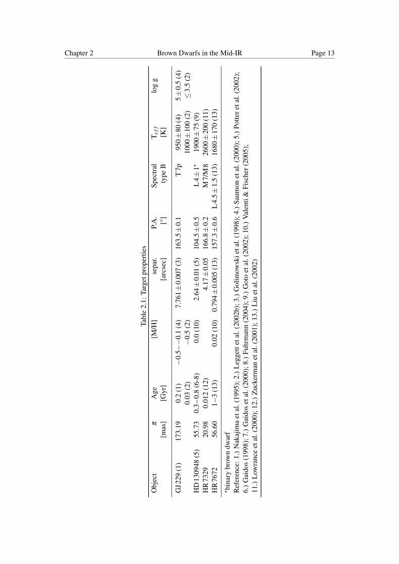
For our target selection, we only considered the confirmed members of binary (or multiple)systems with known distances, as their primaries are well characterized in terms of metallicityand age. Only BD companions with expected mid-IR fluxes stronger than 1mJy and separa-tions larger then 0.5arcsec were selected, in order to fully adapt and exploit the sensitivityand spatial resolution of the mid-infrared imager VISIR at the VLT. We finished with a shortlist of four systems: GJ229, HD130948, HR7329 and HR7672. Their main characteristicsare summarized in Table 2.1.

• GJ229B is the first unambiguous BD discovered (Nakajima et al. (1995)). Later on, or-bital motion was detected by Golimowski et al. (1998), who observed GJ229B at threeepochs spread over approximately one year using HST’s Wide Field Planetary Camera2 (WFPC2). Matthews et al. (1996) derived an effective temperature of 900K from themeasured broadband spectrum of GJ229B, assuming a radius equal to that of Jupiter.The same effective temperature was obtained by Leggett et al. (1999) by comparingcolours and luminosity to evolutionary models developed by Burrows et al. (1997). Ingeneral model spectra for GJ229B (Marley et al. (1996); Allard et al. (1996)) repro-duce the overall energy distribution fairly well and agree with Te f f =950K.

• HD130948BC is a binary brown dwarf companion detected by Potter et al. (2002).The separation between the two companions is (0.134±0.005)arcsec at PA=(317±1)°.Both companions have the same spectral type (L4±1) and effective temperatures(Te f f = (1900±75)K, Goto et al. (2002)).

• HR7329B is a BD companion detected by Lowrance et al. (2000) at a separation of 4”from the early-type star HR7329A, a member of the β Pictoris moving group (Zucker-man et al. (2001)). Its optical spectrum points towards a spectral type M7/M8 and aneffective temperature of 2405 to 2770K for this young substellar companion. Guentheret al. (2001) presented evidence that the source is a co-moving companion.

• HR7672B, a common proper motion companion to the variable star HR7672A, wasreported by Liu et al. (2002). They inferred an effective temperature of Te f f =1510–1850K for HR7672B and estimated an age of 1–3Gyr for the system.

All targets were observed using VISIR mounted at the UT3 (Melipal) with the filters PAH1(λcen =8.59 µm, ∆λ =0.42 µm), PAH2 (λcen =11.25 µm, ∆λ =0.59 µm) and SIV (λcen =10.49 µm,∆λ =0.16 µm). A nominal pixel scale of 0.075” was used during all observations, and stan-dard chopping and nodding techniques were employed, with a chop-throw amplitude of 6”and 8” for GJ229, and a chopping frequency of 0.25Hz. The nodding direction was chosen


Tabl

e2.

1:Ta

rget

prop

ertie

sO

bjec

tπ

Age

[M/H

]se

par.

P.A

.Sp

ectr

alT

eff

log

g[m

as]

[Gyr

][a

rcse

c][°

]ty

peB

[K]

GJ2

29(1

)17

3.19

0.2

(1)

−0.

5–−

0.1

(4)

7.76

1±

0.00

7(3

)16

3.5±

0.1

T7p

950±

80(4

)5±

0.5

(4)

0.03

(2)

−0.

5(2

)10

00±

100

(2)≤

3.5

(2)

HD

1309

48(5

)55

.73

0.3

–0.

8(6

-8)

0.0

(10)

2.64±

0.01

(5)

104.

5±

0.5

L4±

1?19

00±

75(9

)H

R73

2920

.98

0.01

2(1

2)4.

17±

0.05

166.

8±

0.2

M7/

M8

2600±

200

(11)

HR

7672

56.6

01

–3

(13)

0.02

(10)

0.79

4±

0.00

5(1

3)15

7.3±

0.6

L4.

5±

1.5

(13)

1680±

170

(13)

?bi

nary

brow

ndw

arf

Ref

eren

ce:1

.)N

akaj

ima

etal

.(19

95);

2.)

Leg

gett

etal

.(20

02b)

;3.)

Gol

imow

skie

tal.

(199

8);4

.)Sa

umon

etal

.(20

00);

5.)

Potte

reta

l.(2

002)

;6.

)G

aido

s(1

998)

;7.)

Gai

dos

etal

.(20

00);

8.)

Fuhr

man

n(2

004)

;9.)

Got

oet

al.(

2002

);10

.)V

alen

ti&

Fisc

her(

2005

);11

.)L

owra

nce

etal

.(20

00);

12.)

Zuc

kerm

anet

al.(

2001

);13

.)L

iuet

al.(

2002

)


parallel to the chopping direction and, consequently, with an equal nodding to chopping am-plitude.To ensure that the primary and the companion are within the FoV during chopping and nod-ding, the system was aligned horizontally on the detector. At the same time, this simplifiesthe reduction process, since the shifting and adding of the frames can be done using thebrighter primary star. A summary of the observing log is given in Table 2.2, including themean airmass during the observing run and the total integration time.

2.2.3 Data Reduction

The reduction was done using self-written IDL routines for bad-pixel replacement and forthe shifting and adding of the frames. Bad-pixels were replaced by the mean value of thesurrounding pixels within a box of 9×9 pixel, before subtracting (A-B) nodding positions.In the following, the relative shifts between the frames of one data-set were calculated viacross-correlation of the bright primary, before the frames were averaged. Since the VISIR de-tector was affected by randomly triggered stripes during part of the observations, a destripingtechnique developed by Pantin et al. (2007) was applied to the final co-added images.

2.2.3.1 Aperture Photometry

Standard aperture photometry was used to determine the relative photometry of all detectedBDs. Using IDL ATV routines, a curve-of-growth method was applied to the brown dwarfcompanions to obtain the apertures where the signal-to-noise ratio is maximised. In thefollowing, those apertures were used for the primary as well as for the standard stars. Thusthe count-rate to flux conversion factor was determined and relative photometry obtained.The variation of the count-rate to flux conversion factors with aperture radius was screenedfor at least 3 consecutive aperture radii between 4 and 7 pixels (corresponding to radii of0.3” to 0.525q). At 10 µm the VISIR diffraction limit is 0.3”, the chosen aperture radii areof the order or twice the diffraction limit. To calibrate the flux values different standardstars1, observed before and after the targets, were used. The error bar estimation of the fluxcalibration is derived from the flux variations of the source measured in different aperturesand from different standard stars. In cases where two independent measurements were taken,an average of the measured fluxes is quoted in Table 2.4.

As already mentioned, a destriping technique was applied to the final images to cleanit of random stripes and thereby improve the image quality. To estimate the impact of thedestriping on the photometry of the BDs, we performed the aperture photometry before andafter the destriping process. In those cases in which the source is not located close to astripe, no influence is noticeable. In contrast, in the cases where the BD is close to a stripe,a decrease in the measured count-rate, and consequently in flux, of the BD in the destripedimages is perceivable. Nevertheless, this effect is expected, since the stripes in the "raw"images fall within the aperture radii and lead to an overestimation of the count-rate andtherefore of the flux.

1Taken from the list of Cohen et al. (1999)


Tabl

e2.

2:O

bser

ving

Log

Obj

ect

Filte

rU

Tda

teA

irm

ass

DIM

Ma

hum

idity

DIT

ND

IT#

ofIn

t.tim

edC

alib

rato

rdd

/mm

/yr

seei

ng[”

][%

][s

]no

dsc

[s]

GJ2

29PA

H1

08/0

1/06

b1.

109

0.91

17–

500.

016

123

1221

72.7

HD

2696

7,H

D75

691

10/0

2/06

b1.

195

0.79

23–

550.

016

123

1832

59.

HD

4104

7,H

D75

691

PAH

203

/02/

06b

1.04

40.

8320

–40

0.00

824

66

1086

.3H

D41

047,

HD

2696

710

/02/

061.

110

0.84

23–

550.

008

246

610

86.3

HD

2696

7,H

D75

691

SIV

10/0

2/06

1.02

20.

9523

–55

0.04

4811

1943

.H

D26

967,

HD

7569

1H

D13

0948

PAH

109

-10/

07/0

61.

524

0.67

6–

80.

0298

2239

67.

HD

1337

74,H

D99

167

PAH

211

/07/

06b

1.54

10.

917

–10

0.01

197

2239

87.3

HD

1490

0904

-05/

08/0

6b1.

734

0.71

70.

0119

711

1993

.6H

D14

9009

,HD

1458

97SI

V03

/08/

061.

627

0.86

5–

80.

0448

1119

43.

HD

1458

9705

/08/

061.

606

0.62

6–

110.

0448

1119

43.

HD

1458

97H

R73

29PA

H1

07/0

606

1182

1.05

4–

120.

0298

2239

67.

HD

1783

45PA

H2

21/0

5/06

1.15

31.

367

–19

0.00

824

611

1991

.6H

D17

8345

SIV

07/0

6/06

1.17

50.

884

–12

0.04

4822

3886

.1H

D17

8345

HR

7672

PAH

110

/07/

06b

1.34

10.

766

–8

0.02

9811

1983

.5H

D18

9695

,HD

1490

0912

/07/

06b

1.40

50.

886

–11

0.01

612

311

1991

.6H

D18

9695

,HD

1783

45PA

H2

10/0

7/06

b1.

385

0.81

6–

80.

0119

711

1993

.6H

D18

9695

,HD

2209

5413

/07/

06b

1.69

30.

785

–8

0.01

197

1119

93.6

HD

1980

48,H

D21

7902

SIV

13/0

7/06

b1.

356

0.82

5–

80.

0448

1526

49.6

HD

1783

45,H

D19

8048

a.)

inV

band

at55

0nm

,b.)

data

show

edst

ripe

s,c.

)23

chop

spe

rnod

,d.)

t=D

IT×

ND

IT×

#of

chop

s×#

ofno

ds×

4


Figure 2.6: VISIR detection images of GJ299B at ∼6.8” (upper), HR7329B at ∼4.3”(middle) and HD130948BC at∼2.5” (bottom) at 8.6 µm. To all images a σ filter with a boxwidth of 5 pixel has been applied. Furthermore the N–E orientation of the data is over-plottedin the lower right corner of each image.

2.2.3.2 Detection Limits

To estimate the detection limits as a function of angular separation two approaches were ex-plored. The standard deviation of the intensities within a 1 pixel wide annulus at a givenradius was determined, as well as the standard deviation within a box of 5×5 pixels alonga random radial direction. Using the obtained noise estimate, the contrast with respect tothe peak intensity of the primary was calculated (see, e.g., Figure 2.8). The detection limitsdelivered by both methods are in good agreement. Additionally, to further test the derived de-tection limits, artificial companions, with fluxes varying between 2 and 10mJy, were placedwithin the data at separations between 1” and 5”. The limiting fluxes of the re-detectable ar-tificial companions match the previously derived detection limits. Up to a separation of 1.5”the detection limit is dominated by the photon noise of the central star, and at larger separa-tion the background noise from the atmosphere and the instrument limits our detections.


Figure 2.7: VISIR images of HD130948 in the SIV filter taken on the 5th of August (left) andon the 3rd of August (middle). The binary brown dwarf companion was detected in the datafrom the 5th of August and is marked by a box. The flux was measured to be 5.7±0.4mJy.In the data set from the 3rd of August the companion was not detected. Its approximatelocation is at the same position as in the left image and also marked by a box. The rightimage shows the data from the 3rd of August, in which an artificial companion of 4mJy hasbeen placed. The artificial companion is located somewhat below the expected position ofthe real companion.

2.2.4 Results

Three of the four brown dwarfs were detected in PAH1, namely GJ229B, HR7329B andHD130948BC (see Figure 2.6), while only HD130948BC could be detected in SIV. Notethat HD130948BC, a binary brown dwarf, was not resolved in our observations. HR7672Bcould not be detected in any of the filters. While the resolution of VISIR is sufficient toseparate the brown dwarf and the primary (0.79” - Liu et al. (2002); assuming negligibleorbital motion), the data quality in PAH1 and SIV is low. The PSF of the primary is elongated,affecting the area in which the brown dwarf is expected, and thus adding noise.

Table 2.3: Separations and position angles of the detected brown dwarfs.Object UT date sep. [”] P.A. [°]

GJ229 10/02/06 6.78±0.05 168.4±0.9HD130948 09/07/06 2.54±0.05 103.9±2.4

HR7329 07/06/06 4.17±0.11 167.2±1.4

In Table 2.3 the measured separations and position angles of the detected brown dwarfsare given. To obtain the separation as well as the position angle of the brown dwarfs rela-tive to their primaries, the pixelscale and N-orientation provided in the image header wereused. Golimowski et al. (1998), used the HST’s Wide Field Planetary Camera 2 (WFPC2) toobserve GJ229B at three epochs, which were spread over approximately one year. Orbitalmotion of GJ229B was detected and a relative change of separation of (0.088±0.010)” peryear was measured. In the last 10 years, from November 1996 to February 2006, the separa-tion between GJ229A and B changed by (0.894±0.05)”, resulting in an average change ofseparation of (0.097±0.005)” per year. For HD130948, only a minor change of separationis observable. From February 2001 to July 2006 the separation between HD130948A andBC decreased by (0.09±0.05)”. In the case of HR7329 no orbital motion was observable.In Table 2.4 the obtained fluxes for the primary stars and the brown dwarfs, and the upperlimits for the non-detections, are listed. In the case of HD130948BC the flux measured in


the data set from the 5th of August is quoted, as well as the upper limit obtained on the 3rdof August. While the observations of HD130948BC in SIV have been carried out at twodifferent epochs, on the 3rd and the 5th of August, the object was only detectable in thesecond data set (see Figure 2.7) with a measured flux of (5.7±0.4)mJy. The non-detectionof HD130948BC in the data set from the 3rd of August can not be explained by a discrep-ancy in the sensitivity limits, see Figure 2.8. Both data sets clearly reach the same sensitivitylimit. Furthermore, simulations of artificial sources showed that a companion with a flux of(4±0.4)mJy (corresponding to a 5σ confidence level) would have been detected in both datasets. Hence, within ∼48 hours HD130948BC varied by at least (1.7±0.6)mJy.

Table 2.4: VISIR photometry of the primaries and brown dwarfs. In case of a non-detectionupper limits are provided. The fluxes are quoted in mJy.

Object PAH1 SIV PAH2

GJ229A 1297. (47.) 923. (33.) 793. (26)GJ229B 3.2 (0.5) 2. (0.3) 4. (0.9)a

HD130948A 861. (5.) 605. (27.)b 478. (6.)HD130948BC 3.8 (0.4) 5.7 (0.4)b 1.8 (0.2)a

HD130948A 553. (27.)c

HD130948BC 2. (0.4)a,c

HR7329A 524. (19.) 404. (3.) 386. (24.)HR7329B 3.2 (2.3) 1.3 (0.2)a 2.3 (0.2)a

HR7672A 880. (36.) 554. (33.) 519. (14.)a.) limiting background (1σ ), b.) 05/08/06, c.) 03/08/06

2.2.5 Discussion

2.2.5.1 Comparison with Models

As a final step we compare our obtained photometry to the models developed by Allard et al.(2001) and Burrows et al. (2006). Using their theoretical spectra, provided online2, absolutemodel fluxes were calculated by integrating the theoretical spectrum over the VISIR filterbandpasses. The object radii R, which determine the absolute spectral flux calibration, wereobtained from evolutionary calculations by Burrows et al. (1997). In Table 2.5 the calculatedmodel fluxes are listed. Furthermore, the age and effective temperature combinations forwhich the object radius was determined are given. From Allard et al. (2001) we employed theAMES-cond and AMES-dusty models, representing the two extreme cases, in which eitherall dust has disappeared from the atmosphere (AMES-cond) or dust settling throughout theatmosphere is negligible (AMES-dusty). Following Allard et al. (2001) the AMES-dustymodels should successfully describe dwarfs with effective temperatures greater than 1800K,while the AMES-cond models are better suited to describe the atmospheres of dwarfs withTe f f ≤1300K.

GJ229B: Saumon et al. (2000), have used high-resolution infrared spectra to determinethe metallicity, effective temperature and gravity of the T dwarf (see also Table 2.1). Whileusing an age of 0.2Gyr they derived an effective temperature of 950K±80K and a gravity

2http://perso.ens-lyon.fr/france.allard/ and http://zenith.as.arizona.edu/burrows/

Chapter 2 Brown Dwarfs in the Mid-IR Page 19Ta

ble

2.5:

Pred

icte

dm

id-I

Rflu

xes

from

diff

eren

tthe

oret

ical

mod

els.

Val

ues

cons

iste

ntw

ithin

3σ

orw

ithth

egi

ven

uppe

rlim

itar

em

arke

din

bold

face

.O

bjec

tR

efer

ence

Tef

flo

gg

[M/H

]ag

eR

/R�

PAH

1SI

VPA

H2

[K]

[cm

/s2 ]

Myr

[mJy

][m

Jy]

[mJy

]

GJ2

29B

Alla

rda

900

5.0

0.0

200

0.12

23.

302.

975.

06A

llard

a10

005.

00.

020

00.

122

4.67

4.55

6.68

Alla

rda

1000

3.0

0.0

200

0.12

24.

806.

697.

94A

llard

a10

003.

00.

030

0.13

35.

707.

959.

44B

urro

wsc

900

5.0

0.0

200

0.12

23.

353.

04.

25B

urro

wsc

900

5.0

−0.

520

00.

122

3.33

2.46

3.78

Bur

row

sc10

005.

0−

0.5

200

0.12

24.

253.

444.

77B

urro

wsc

1000

5.0

−0.

530

0.13

35.

044.

095.

66B

urro

wsc

1000

4.5

−0.

530

0.13

35.

144.

996.

05m

easu

red

3.2±

0.5

3.21

6.71

HD

1309

48B

CA

llard

b19

005.

00.

080

00.

091

1.65

1.25

1.13

Alla

rdb

1900

5.0

0.0

300

0.10

22.

071.

571.

42A

llard

b19

003.

50.

030

00.

102

1.67

1.21

1.11

Bur

row

sd19

005.

00.

030

00.

102

1.53

1.26

1.17

Bur

row

sd19

005.

0-0

.530

00.

102

1.49

1.25

1.16

mea

sure

d1.

9±

0.3

2.9±

0.33

1.21

mea

sure

d1.

51

HR

7329

BA

llard

b24

004.

00.

012

0.19

31.

060.

910.

79A

llard

b26

003.

50.

08

0.27

82.

802.

302.

55A

llard

b26

003.

50.

012

0.22

91.

901.

561.

73A

llard

b26

004.

00.

012

0.22

91.

761.

441.

25A

llard

b28

004.

00.

012

0.26

52.

842.

201.

91m

easu

red

3.2±

2.3

1.91

2.91

a.)

AM

ES-

cond

mod

els

from

Alla

rdet

al.(

2001

)1.

)up

perl

imit,

limiti

ngba

ckgr

ound

plus

3σ

b.)

AM

ES-

dust

ym

odel

sfr

omA

llard

etal

.(20

01)

2.)

flux

ofon

eco

mpo

nent

assu

min

gbo

thL

4dw

arfs

c.)

L&

Tcl

oud-

free

mod

els

from

Bur

row

set

al.(

2006

)co

ntri

bute

equa

llyto

the

mea

sure

dflu

xd.

)L

&T

mod

elw

ithcl

ouds

from

Bur

row

set

al.(

2006

)3.

)on

ly05

.08.

2006


Figure 2.8: Comparison of the limiting background obtained from the two data sets ofHD130948 taken in the SIV filter. The over-plotted point corresponds to the detection onthe 5th of August, with a flux of 5.7mJy.

of logg=5±0.5. Later on, Leggett et al. (2002b) compared the observed low- and high- res-olution spectra of GJ229A and GJ229B to theoretical spectra (AMES-models). Their bestfit yields an Te f f =1000±100 and a gravity of logg ≤3.5 for GJ229B, as well as a metal-licity of [M/H]≈ −0.5 and an age of ∼30Myr (range 16–45Myr) for the system. While themetallicity is determined within the spectra fitting procedure, the age is derived by a com-parison with evolutionary models, and mainly constrained by the observed luminosity andthe derived effective temperature of the A component. Using VISIR mid-IR photometry, ab-solute model predictions of both Allard et al. (2001) and Burrows et al. (2006) can then betested for different combinations of Te f f , [M/H] and gravity (when available, e.g. see Figure2.9). From Table 2.5, we see that the PAH1, SIV and PAH2 photometry are consistent withmodel predictions for a Te f f =900K, logg=5.0 and [M/H]=0 companion. At solar metallic-ity, an effective temperature of Te f f =1000K can be excluded at more than 2σ . At subsolar[M/H]=−0.5 metallicity, low gravity (logg<4.5) values remain excluded for Te f f =1000K.Therefore, excluding young ages predictions of Leggett et al. (2002b), the VISIR photometryclearly favours the initial physical parameters proposed by Saumon et al. (2000) for solar andsubsolar metallicities

HD130948BC: As already mentioned, HD130948BC is a binary brown dwarf consist-ing of two L4 dwarfs. To compare our observations to the model predictions, we assumedthat both brown dwarfs contribute equally to the measured fluxes, as the simplest assumption.An unequal distribution of the measured flux on one of the two brown dwarfs would onlyincrease the afterwards described effect. The suggested effective temperature of ∼1900Kplaces the binary in the regime of the AMES-dusty models. While the predicted PAH1 fluxis in good agreement with our measurements, most models fail to reproduce the SIV flux


Figure 2.9: GJ229B: Comparison of theoretical spectra from Allard et al. (2001) and Bur-rows et al. (2006) with the VISIR photometry.

detected on August, 5. 2006, but would be consistent with the non-detection on August, 3.2007. Using the models provided by Burrows et al. (2006) we tested the influence of differentmetallicities ([M/H]=0.0 and [M/H]=−0.5) on the predicted fluxes. The change is marginal,only about 0.05mJy.

2.2.5.2 HD130948BC: Photometric Variability

While analysing the SIV data obtained for HD130948, we found that the binary companionwas detectable in only one of the two data sets. A possible explanation of this result is anintrinsic variability around 10.5 µm of one or both of the L dwarfs in the binary. Variabilityat 10.5 µm could either be caused by ammonia (NH3) or silicates. Since the NH3 absorptionfeatures, which were first identified in the mid-infrared spectra taken with Spitzer/IRAS byRoellig et al. (2004), and Cushing et al. (2006), appear at roughly the L/T transition this isunlikely to be the cause of the observed variability. A more favourable explanation may bean inhomogeneous distribution of silicate clouds, which characterise the atmospheres of Ldwarfs with effective temperatures of roughly 1400–2000K (Burrows et al. (2001)). FutureVISIR observations of HD130948BC at 10.5 µm over different timescales should secure thisphotometric variability.


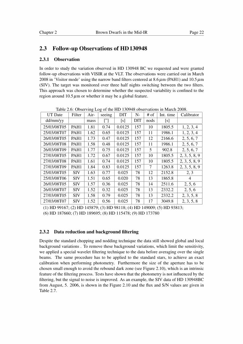
2.3 Follow-up Observations of HD130948

2.3.1 Observation

In order to study the variation observed in HD 130948 BC we requested and were grantedfollow-up observations with VISIR at the VLT. The observations were carried out in March2008 in ’Visitor mode’ using the narrow band filters centered at 8.6 µm (PAH1) and 10.5 µm(SIV). The target was monitored over three half nights switching between the two filters.This approach was chosen to determine whether the suspected variability is confined to theregion around 10.5 µm or whether it may be a global feature.

Table 2.6: Observing Log of the HD 130948 observations in March 2008.UT Date Filter Air- seeing DIT N- # of Int. time Calibrator

dd/mm/yy mass [”] [s] DIT nods [s]25/03/08T05 PAH1 1.81 0.74 0.0125 157 10 1805.5 1, 2, 3, 425/03/08T07 PAH1 1.62 0.65 0.0125 157 11 1986.1 1, 2, 3, 426/03/08T05 PAH1 1.73 0.47 0.0125 157 12 2166.6 2, 5, 6, 726/03/08T08 PAH1 1.58 0.48 0.0125 157 11 1986.1 2, 5, 6, 726/03/08T09 PAH1 1.77 0.75 0.0125 157 5 902.8 2, 5, 6, 727/03/08T05 PAH1 1.72 0.67 0.0125 157 10 1805.5 2, 3, 5, 8, 927/03/08T08 PAH1 1.61 0.74 0.0125 157 10 1805.5 2, 3, 5, 8, 927/03/08T09 PAH1 1.84 0.83 0.0125 157 7 1263.8 2, 3, 5, 8, 925/03/08T05 SIV 1.63 0.77 0.025 78 12 2152.8 2, 325/03/08T06 SIV 1.51 0.65 0.020 78 13 1865.8 426/03/08T05 SIV 1.57 0.36 0.025 78 14 2511.6 2, 5, 626/03/08T07 SIV 1.52 0.32 0.025 78 13 2332.2 2, 5, 627/03/08T05 SIV 1.58 0.79 0.025 78 13 2332.2 2, 3, 5, 827/03/08T07 SIV 1.52 0.56 0.025 78 17 3049.8 2, 3, 5, 8(1) HD 99167; (2) HD 145879; (3) HD 98118; (4) HD 149009; (5) HD 93813;(6) HD 187660; (7) HD 189695; (8) HD 115478; (9) HD 173780

2.3.2 Data reduction and background filtering

Despite the standard chopping and nodding technique the data still showed global and localbackground variations . To remove these background variations, which limit the sensitivity,we applied a special wavelet filtering technique to the data before averaging over the singlebeams. The same procedure has to be applied to the standard stars, to achieve an exactcalibration when performing photometry. Furthermore the size of the aperture has to bechosen small enough to avoid the rebound dark zone (see Figure 2.10), which is an intrinsicfeature of the filtering process. Tests have shown that the photometry is not influenced by thefiltering, but the signal to noise is improved. As an example, the SIV data of HD 130948BCfrom August, 5. 2006, is shown in the Figure 2.10 and the flux and S/N values are given inTable 2.7.


Table 2.7: Example of the measured photometry and the signal to noise before (4th and 5thcolumn) and after (6th and 7th column) wavelet filtering. The values quoted in brackets arethe uncertainties of the flux arising due to different standard stars.

Object date filter flux S/N flux S/N[ddmmyy] [mJy] [mJy]

GJ 229 B 080106 PAH1 3.0 (0.3) 2.5 2.6 (0.4) 5.2100206 PAH1 2.9 (0.3) 1.6 4.7 (0.3) 5.2

HD 130948 BC 100706 PAH1 3.8 (0.4) 4.8 3.4 (0.2) 8.5050806 SIV 5.7 (0.4) 2.9 5.6 (0.4) 6.2

HR 7329 B 070606 PAH1 2.6 (0.2) 3.2 2.3 (0.2) 4.6

Figure 2.10: Comparison of the image quality before and after the background removal byfiltering.

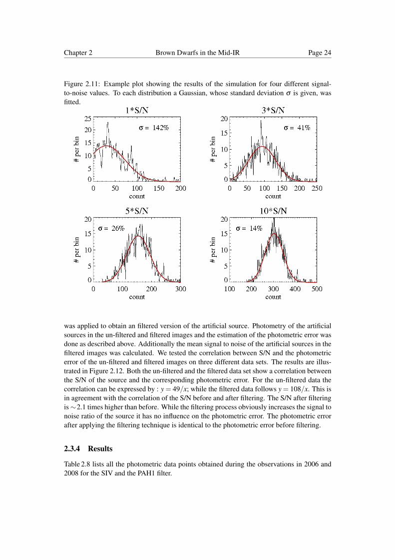
2.3.3 Simulations

To evaluate the photometric error of each independent observation, we performed extensivesimulation, placing artificial sources into the data3. As artificial source the PSF of an as-sociated standard star, scaled to the required signal-to-noise (S/N) was taken and placed atrandomly determined positions. These coordinates are stored and passed on to the automaticphotometry program, which is based on the IDL/ATV routine. For all data sets simulationsfor a variety of S/N values were run with a total of 1.000 artificial sources per S/N value. Incase the positions of the artificial source overlaps with a beforehand defined area around thecoordinates of HD 130948A and HD 130948BC, the result of the photometry is rejected.Thus the number of valid photometric points is reduced too about 600 to 650. The remainingpoints are binned in an histogram and a Gaussian function is fitted to the distribution, seeFigure 2.11. The standard deviation of the Gaussian fit is taken as the photometric error ofthe corresponding S/N level.

In a second step we run simulations following the described approach to evaluate the influ-ence of the background filtering on the signal to noise and the photometric error of a potentialsource. Therefore artificial sources with known signal to noise were placed in the reduced un-filtered images. After placing the artificial source in the data, the wavelet filtering technique

3Completely reduced image on which photometry was performed.


Figure 2.11: Example plot showing the results of the simulation for four different signal-to-noise values. To each distribution a Gaussian, whose standard deviation σ is given, wasfitted.

was applied to obtain an filtered version of the artificial source. Photometry of the artificialsources in the un-filtered and filtered images and the estimation of the photometric error wasdone as described above. Additionally the mean signal to noise of the artificial sources in thefiltered images was calculated. We tested the correlation between S/N and the photometricerror of the un-filtered and filtered images on three different data sets. The results are illus-trated in Figure 2.12. Both the un-filtered and the filtered data set show a correlation betweenthe S/N of the source and the corresponding photometric error. For the un-filtered data thecorrelation can be expressed by : y = 49/x; while the filtered data follows y = 108/x. This isin agreement with the correlation of the S/N before and after filtering. The S/N after filteringis∼2.1 times higher than before. While the filtering process obviously increases the signal tonoise ratio of the source it has no influence on the photometric error. The photometric errorafter applying the filtering technique is identical to the photometric error before filtering.

2.3.4 Results

Table 2.8 lists all the photometric data points obtained during the observations in 2006 and2008 for the SIV and the PAH1 filter.


Figure 2.12: The three graphs display the correlations between the signal-to-noise (S/N) andthe photometric error before and after the background filtering.Upper graph: data points in black are before filtering, those in green are after filtering.


Table 2.8: The table states the fluxes, background limiting sensitivities and the signal tonoise (S/N) measured for all observations of HD 130948BC. The measurements wereobtained after applying the background filtering technique to all observation from 2006 and2008. In red: 3σ upper limits.

date filter flux simu bg limit S/Ndd/mm/yy [mJy] [%] [mJy]10/07/06 PAH1 3.4 (0.2) 12. 0.4 8.503/08/06 SIV 2.7 41. 0.9 3.05/08/06 SIV 5.6 (0.4) 19. 1.0 6.2

25/03/08T05 PAH1 2.4 (0.5) 80. 1.4 1.725/03/08T07 PAH1 4.4 (0.7) 25. 1.2 3.726/03/08T05 PAH1 4.0 (0.4) 21. 0.8 5.026/03/08T08 PAH1 3.6 (0.4) 25. 1.0 3.626/03/08T09 PAH1 3.7 (0.5) 38. 1.2 3.127/03/08T05 PAH1 3.9 (0.4) 39. 0.9 4.327/03/08T08 PAH1 3.9 (0.4) 28. 1.0 3.927/03/08T09 PAH1 4.2 (0.5) 30. 1.1 3.825/03/08T05 SIV 4.3 (0.5) 55. 2.2 2.025/03/08T06 SIV 5.7 32. 1.9 3.26/03/08T05 SIV 3.9 35. 1.3 3.26/03/08T07 SIV 3.6 26. 1.2 3.27/03/08T05 SIV 3.6 (0.3) 43. 1.4 2.627/03/08T07 SIV 2.8 (0.2) 51. 1.1 2.6


Table 2.9: Parameters put into and results obtained form the variability tests.Filter N f f ∗ χ2 p η

PAH1 9 3.72 3.90 1.79 98.7 0.41SIV 4 4.08 3.95 2.95 39.9 0.91SIV 8 4.03 3.75 5.51 59.8 0.72

To test whether the photometric measurements show evidence of variability we used twostatistic approaches. The first is the χ2 test:

χ2 =

i=N

∑i=1

(fi− f

σi)2 (2.1)

• fi - flux of measurement i

• σi - photometric error of measurement i

• f - mean flux of all measurements

• N - number of measurements

It evaluates the probability that the deviations of the photometric points are consistent withthe photometric errors (Bailer-Jones & Mundt (1999), Morales-Calderón et al. (2006)). Thenull hypothesis for the test is that there is no variability. Form the yielded χ2 the probability(p) that the null hypothesis is true can be determined (look up tables). Thereby a large χ2

indicates a greater deviation and thus a smaller p. If p < 0.01 we claim evidence for variability.The second test was introduced by Enoch et al. (2003) as a more robust statistic approach.They defined:

η =1

N−1∗

i=N

∑i=1

| fi− f ∗ |σi

(2.2)

where fi, σi and N are as above and f ∗ is the median flux of all measurements. If η < 1 thanthere is no evidence for variability, while for an η&1 the object is likely to be variable, butMonte-Carlo-Simulations would be necessary to obtain the probability with which the objectis variable. Both statistics implicit the assumption that the random scatter in the observationsis Gaussian, but the η-test is likely to be more robust in case of outliers.

Both tests were applied to each filter. For the SIV data points we calculated the χ2- and theη-test twice. One time only the detected data points were taken into account, disregarding thenon-detections. The second time non-detections were accounted for by using the 3σ upperlimit when calculating χ2 and η . The results from both tests are given in Table2.9. Neitherthe χ2- nor the η-test yields any evidence for variability either in PAH1 or SIV. All threecomputed values for η are well below 1 indicating that the source is not variable. While theprobability calculated from the χ2- test confirms non-variability for PAH1, the result is muchmore uncertain for SIV, but still in favour of non-variability.


Figure 2.13: Sequence of the March 2008 observations of HD 130948BC in PAH1 and SIV.


2.4 Conclusion

Using VISIR at the VLT, we performed a mini-survey of brown dwarfs in binary systems.The four selected brown dwarfs were imaged in three narrow band filters at 8.6, 10.5 and11.25 µm. At 8.6 µm three of the brown dwarfs were detected and photometry was obtained.None of the brown dwarfs was detected at 11.25 µm, and only HD130948BC was detectedat 10.5 µm. The observations of HD130948BC at 10.5 µm indicate a possible variation ofone or both brown dwarfs of the binary.

To constrain the atmospheric properties of the brown dwarfs we compared the mid-infrared photometry to theoretical model spectra by Allard et al. (2001) and Burrows et al.(2006). The measured mid-infrared fluxes and upper limit of GJ229B are consistent with thecharacteristic parameters obtained, by Saumon et al. (2000) (Te f f ∼950K, logg ∼5, respec-tively), while values of the effective temperature and gravity as suggested by Leggett et al.(2002b) (Te f f ∼1000K, logg ≤3.5, respectively) result in too high model fluxes. As forHD130948BC, the model fluxes for Te f f ∼1900K, logg ≤5 fit the measurement at 8.6 µmand the upper limits obtained at 10.5 µm and 11.25 µm. Nevertheless, the models are not inagreement with the flux measured for the detection of HD130948BC at 10.5 µm during oneobserving epoch. The disagreement of the two observation of HD 130948BC at 10.5 µm ledus to request follow-up observation to study the behaviour of the flux of the binary browndwarf in two filters over an extended time interval. The observations yielded eight moredata points in the narrow band filter around 8.6 µm and three detections of HD 130948BC at10.5 µm. In order to analyse whether the variations seen in the fluxes at 8.6 µm and 10.5 µmare statistical relevant we applied two statistic test to both data sets taken in the differentfilters. From the results of both test variability can neither be confirmed in PAH1 nor in SIV.

Chapter 3

Searching for Low-Mass Companionsin the Mid-Infrared

3.1 Motivation

3.1.1 Previous Work

There are numerous surveys which have been or are searching for brown dwarfs and plane-tary companions, but most of them were or are carried out in the near-infrared concentratingon near-by, young stars (Metchev & Hillenbrand (2004), Masciadri et al. (2005), Chauvinet al. (2006), Biller et al. (2007), Neuhäuser et al. (2006)) . Only three projects were or areconducted in the mid-infrared wavelength regime or in the near-infrared L and M bands. Oneof the first attempts was a 10 µm broadband imaging survey carried out by van Buren et al.(1998). Using the Palomar 5 Meter telescope they observed eight near-by stars to search forsub-stellar companions. No detection was achieved, but objects brighter than 10mJy at sep-arations between 2.”-10.” from the primary would have been detectable. For the observedstars this upper flux limit translates into companions just slightly below the hydrogen-burninglimit.More recent surveys have been carried out by Kasper et al. (2007) and Heinze et al. (2006),whereas the last mentioned project is still on-going, with the aim to survey 50 near-by,moderate-aged stars for giant extrasolar planets. The observations are planned to be donein L’- (3.8 µm) and M- (4.8 µm) band using the Clio camera together with adaptive opticssystem on the 6.5m MMT telescope. At these wavelengths giant planets should be evenvisible around near-by, old stars, up to 5.Gyr. So far 7 out of the 50 target stars have beenobserved, and Monte Carlo simulations to demonstrate the ability to detect Jupiter mass plan-ets around them, have been performed. The simulations show that, in special cases, planetsdown to 6. Jupiter masses orbiting an 1.Gyr old star are detectable.Finally, Kasper et al. (2007) observed a small sample of 22 young, nearby stars using theVLT/NACO system in the L band. The target sample is comprised out of members of theTucana association and the β Pic moving group, which ages are estimated to be between 10.and 30.Myr. No companion has been detected, but the observations were sensitive to objectswith masses down to 1.−2MJ at separations larger than 5. to 30.AU.

With the rise of the Spitzer Space Telescope the mid-infrared wavelength regime becameaccessible to direct imaging searches for brown dwarfs and extrasolar planets. An example is

31

Chapter 3 A low-mass Companion Search Page 32

Figure 3.1: Sensitivity limit of ε Eri from the IRAC observation by Marengo et al. (2006).

the survey of 5’×5’ fields surrounding stars in the solar neighbourhood conducted by Luh-man et al. (2007) with the IRAC instrument. As an intermediate result two T dwarf compan-ions to the near-by stars HN Peg and HD 3651 at separations of 43.”2 and 42.”9, respectively,have been announced. But, IRAC should be able to detect even lower mass objects, as shownby the observations of the main sequence star ε Eri (Marengo et al., 2006). Depending on thefilter, sensitivity limits down to 1 Jupiter mass were reached (see Figure 3.1). As a disadvan-tage of the low resolution of the instrument and the required long integration times the areaclosest to the star will naturally be saturated and hence useless for the scientific purpose. Forε Eri a region (cross-hatched in Figure 3.1) within a radius of 14” (45 A.U.) from the star hadto be excluded because of saturation effects and high residual noise after PSF subtraction.

But this drawback opens a niche for ground-based mid-infrared instruments.

3.1.2 Limits

While space-based mid-infrared observatories have the clear advantage of sensitivity com-pared to ground-based instruments, they are limited by the size of the primary mirror. Ground-based 8m class telescopes may not reach the same sensitivity limits as the Spitzer SpaceTelescope, but they have a much higher resolution, which makes them competitive whensearching for companions at small angular separations from the primary star.To get a rough notion of what kind of objects one would expect to detect with either of thetwo mid-infrared images at VLT and GEMINI, one has to combine the nominal sensitivitylimit of the instrument with prediction from theoretical models. The nominal sensitivity lim-


Table 3.1: Predicted fluxes calculated from theoretical models (Allard et al., 2001) assumingan age of 0.5Gyr.

5pc 10pcM M Te f f logg R PAH1 Si5 PAH1 Si5

[M�] [MJ] [K] [R�] [mJy] [mJy] [mJy] [mJy]0.007 7.3 500 4.2 0.112 0.4 1.2 0.1 0.30.010 10.5 600 4.4 0.110 0.9 2.0 0.2 0.50.015 15.7 800 4.6 0.107 2.4 4.2 0.6 1.10.020 21.0 900 4.7 0.104 3.2 5.3 0.8 1.3

Table 3.2: Predicted fluxes calculated from theoretical models (Allard et al., 2001) assumingan age of 1Gyr.


[M�] [MJ] [K] [R�] [mJy] [mJy] [mJy] [mJy]0.0085 8.9 450 4.3 0.107 0.3 0.7 0.07 0.2

0.01 10.5 500 4.4 0.107 0.4 1.1 0.1 0.30.02 21.0 800 4.7 0.100 2.1 3.7 0.5 0.90.03 31.4 1000 4.9 0.096 3.9 5.3 1.0 1.30.04 41.9 1300 5.1 0.093 7.0 7.6 1.7 1.9

its for both VLT/VISIR and GEMINI/T-ReCS are published on the respective web pages.Since only one filter of each instrument will be of interest in the context of this work, thediscussion will be limited to the filters in question. The PAH1 filter, centered at 8.6 µm, ofVISIR is given with a nominal sensitivity limit of 5mJy 10σ /h, while the T-ReCS web pagestates 1.6mJy 5σ /30min (roughtly ∼2.2mJy 10σ /hr) as sensitivity limit for the Si5 filter,centered at 11.7 µm.

Taking theoretical models, like those from Allard et al. (2001), one can calculated the ex-pected mid-infrared fluxes of objects with certain age, mass and effective temperature combi-nations, by integrating the theoretical spectra over the filter passband. Tables 3.1, 3.2 and 3.3

Table 3.3: Predicted fluxes calculated from theoretical models (Allard et al., 2001) assumingan age of 5Gyr.


[M�] [MJ] [K] [R�] [mJy] [mJy] [mJy] [mJy]0.015 15.7 400 4.6 0.098 0.1 0.4 0.03 0.10.030 31.4 600 5.0 0.090 0.9 1.6 0.2 0.40.040 41.9 750 5.2 0.085 1.3 2.1 0.4 0.50.050 52.4 950 5.3 0.082 2.7 3.2 0.7 0.80.060 62.8 1100 5.4 0.079 3.5 4.0 0.9 1.0


list exemplary results of such an exercise. The calculated theoretical fluxes are supposed tobe taken as a guideline to get a feeling for what kind of object should be detectable (markedin bold face in all three tables) in a companion search survey employing ground based tele-scopes.

3.2 Survey

The most stringent limitation of surveys searching for faint companions are residual artefact’sand time varying aberrations in the point-spread-function (PSF) around the bright primaries.One way to overcome the limitations of the optical and near infrared surveys is to observeat longer wavelengths. In the mid-IR (10µm), the residual optical aberrations of the PSFare of much less concern, and for 8m-class telescopes, they can basically be neglected atangular separations larger than 1 arcsec from the primary star. This project aims at detectinglow mass companions to bright, near-by stars, using the mid-infrared facilities VISIR atthe VLT and TReCS at Gemini/South. The favourable flux contrast between the primaryand a potential secondary in the 10 µm regime allows us to search for companions havingtemperatures below 1000K at separations of only 1” to 3” from the primary. E.g., for astar at a distance of 5 parsec from the sun these separations translate to 5-15 AU, a domainhighly interesting for planetary formation, and where orbital periods get too long to makesuch objects easily (i.e. within a short time span) detectable by radial velocity or astrometricmonitoring. We stress that our observations are complementary t other ground or space basedefforts (both direct imaging and indirect methods), since we target a separation region hardto access.

3.2.1 Target Sample

The complete sample of the VISIR and T-ReCS observations is compound of fourteen stars,all selected according to the following three criteria: optical and near-infrared brightness, dis-tance and visibility. Since both the VLT and the GEMINI/South are located on the southernhemisphere, possible targets were required to have declinations southward of +15°. Concern-ing the first criteria the targets were required to be brighter than V=5mag and Ks=3mag,so that they are most likely to be excluded from common optical and near-infrared, directimaging surveys. As a final requirement we wanted the targets to be near-by (<10pc) to beable to resolve companions at physical distance of 5 to 15AU, a domain highly interesting forplanetary formation. Not all targets fullfill this last constraint, which is due to observationaltime constraints and the lack of fitting targets to observe.Three of the observed targets are planet host candidates. One of them is β Hyi a G0 mainsequence star situated at a distance of ∼7.5pc from the Sun. Since 2002 the star is know tohave a linear radial velocity trend (Endl et al., 2002), most likely caused by giant planet orsubstellar companions located at a separation >1”. The remaining two targets are ε Eri andε Ind A, both described in more detail below.

ε Eri : At a distance of only 3.2 pc is ε Eri the nearest star with a detected circumstellardisc (Greaves et al., 1998) and a planet candidate. It has been extensively studied using ra-dial velocity, astrometry and direct imaging techniques. Starting in 1995, Walker et al. (1995)


Tabl

e3.

4:C

ombi

ned

targ

etlis

toft

heV

ISIR

(not

e:V

)and

T-R

eCS

(not

e:T

)obs

erva

tions

.O

bjec

tπ

SpT

age

rang

eV

KIR

AS

note

[mas

][G

yr]

[Gyr

][m

ag]

[mag

]12

µm

[Jy]

Siri

us37

9.21

A1

V0.

178 ;0

.249

0.23−

0.25

9-1

.47

-1.3

914

3.V

εE

ri31

0.74

K2

V0.

857

0.7-

0.93,

4,5,

6,7

3.73

1.78

9.52

V,T

Proc

yon

A28

5.93

F5IV

1.71,

21.

5−1.

91,2

0.34

-0.6

679

.1V

εIn

diA

275.

79K

4V

1.32

0.8−

2.02

4.69

2.24

V,T

τC

et27

4.18

G8

V0.

31 ;7.2

2 ;5.1

3 ;107

0.2−

12.1,

2,7

3.50

1.79

9.56

VA

ltair

194.

45A

7V

1.22

1.1−

1.42

0.77

0.10

33.0

V36

Oph

167.

08K

2V

4.32

5.81

Vδ

Pav

163.

74G

8IV

9.31

5.5−

10.8

13.

561.

937.

67V

βH

yi13

3.78

G0

V5.

213.

5−7.

01,2.

801.

3711

.8T

ζTu

c11

6.38

F9.5

V3.

51 ;6.5

22.

4−10

.71,

24.

202.

773.

18V

βV

ir91

.74

F9V

2.71 ;2

.62 ;4

.53

2.2−

3.21,

23.

612.

275.

22V

βL

eo90

.16

A3

V0.

22 ;0.1

70.

1−0.

42,7

2.14

1.88

6.97

VA

rctu

rus

88.8

5K

1.5

III

-0.0

4-2

.91

793.

VR

efer

ence

s:1.

)H

olm

berg

etal

.(20

07);

2.)

Lac

haum

eet

al.(

1999

);3.

)W

righ

teta

l.(2

004)

;4.

)Sa

ffe

etal

.(20

05);

5.)

Hen

ryet

al.(

1996

);6.

)So

nget

al.(

2000

);7.

)D

iFol

coet

al.(

2004

);8.

)R

ieke

etal

.(20

05);

9.)

Lie

bert

etal

.(20

05);

10.)

Port

ode

Mel

loet

al.(

2008

)


presented radial velocity observations suggesting a planet candidate in an about ten year longorbit around ε Eri. Three years later, Cumming et al. (1999) published radial velocity datataken with the Lick Observatory showing also significant variations, but with a period ofonly 6.9 years. Combining all the existing radial velocity observations with additional datafrom the McDonald Observatory Planet Search Program (Cochran & Hatzes, 1993), Hatzeset al. (2000) confirmed the presence of long period radial velocity variations most likely tobe explained by a planetary companion with a period of 6.9 years. Additional evidence forthe planetary companion ε Eri b comes from the astrometric observations spanning a to-tal time of about 15 years (Benedict et al., 2006). In combination with the radial velocitydata the authors determined for ε Eri b a period of 6.85±0.03 yr, a perturbation semimajoraxis of α =1.88±0.2 mas and an inclination of i=30.1°±3.8°. This inclination is consistentwith the disc inclination determined by Greaves et al. (2005). Assuming a stellar mass ofM? =0.83M� for ε Eri A, Benedict et al. (2006) calculate a mass of M=1.55MJ±0.24MJ

for ε Eri b. Furthermore, the radial velocity data seems to indicate a long-term linear trend,consistent with a Jupiter-mass object at larger separations (P ~50−100 yr). The suggestionthat ε Eri may harbour a second planet has already been made by Deller & Maddison (2005).They speculated, that a a second planet, ε Eri c may have shaped the discs morphology.

ε Ind : The system consists of a K4 main sequence star and a binary brown dwarf com-panion at a projected separation of about 1460 AU. The physical companion, dupped ε IndBaBb, has been discovered in 2003 (Scholz et al., 2003) and was soon afterwards foundto be a binary consisting of two T dwarfs (Volk et al. (2003), McCaughrean et al. (2004)).The two components have spectral types of T1 and T6 and estimated masses of 47±10MJ

and 28±7MJ , respectively, assuming an age of 1.3Gyr for the system (McCaughrean et al.,2004). However, new astrometric monitoring data of the ε Ind system points towards a muchhigher total mass of 121MJ for the brown dwarf binary (Cardoso et al., 2008), implying thatthe system may be as old as 5Gyr.Furthermore, radial velocity data of ε Ind A shows a linear trend most likely caused by adistant stellar companion as well as by a very long-period (P > 20 yrs) planetary compan-ion (Endl et al. (2002)). The observations were carried out with the ESO Coudé EchelleSpectrometer (CES) on La Silla. The best-fit to the RV measurements gives an RV shift of0.012±0.002 m/s per day. The rms scatter around the slope is given as 11.6m/s. Until now novisual companion has been found and, even a deep search with VLT/NACO in H and Ks didnot reveal a companion (Geißler et al. (2007)). The observations were limited to objects withH<16. mag and Ks<15.6 mag at a separation of 3”. Applying theoretical models (Baraffeet al., 2003) the limiting magnitudes were converted into a lower mass limit of 15MJ , assum-ing a system age of 1Gyr. Thus, the yet unidentified radial velocity companion of ε Ind A ismost likely substellar.

3.2.2 Observations and Data Reduction

As already mentioned observations were carried out using the mid-infrared facilities at theVLT (VISIR) and the GEMINI/South (T-ReCS).


Table 3.5: Log of the GEMINI/ T-ReCS observations.Target Date P.A. Airmass FRM time Int. time Calibrator note

ddmmyy [%] [ms] [s]ε Eri 010907 0. 1.147 25.856 926.67 HD23249ε Eri 010907 20. 1.082 25.856 926.67 HD23249ε Ind 160807 0. 1.120 25.856 926.67 HD211416 set1ε Ind 160807 340. 1.156 25.856 926.67 HD211416 set1ε Ind 210807 0. 1.122 34.474 926.67 HD211416 set2ε Ind 210807 340. 1.167 34.474 926.67 HD211416 set2β Hyi 270807 0. 1.571 25.856 926.67 HD224889 set1β Hyi 270807 20. 1.509 25.856 926.67 HD224889 set1β Hyi 270807 0. 1.465 25.856 926.67 HD224889 set2β Hyi 270807 20. 1.464 25.856 926.67 HD224889 set2

GEMINI/South : The Observations with T-ReCS were conducted in August and Septem-ber 2007 in service mode. Each target was imaged at two different instrument angles sepa-rated by 20° in the Si5 broad band filter centered at 11.7 µm. Table 3.5 lists the basic set-upparameters and observing conditions for all T-ReCS observations. During the observationsthe nodding direction was chosen to be parallel, with a nod and chop throw of 15 arcsec. Thechopping angle was tilted between 30° and 50° east of north, so that per chopping cycle thetelescope was only half the time on source. Background removal was done by subtracting theframes of corresponding chopping positions of each nod position and afterwards subtract-ing the images from the two corresponding nodding positions. The final step is to align andaverage all frames of each observation block.

VLT : The observations with the VISIR instrument were conducted during two nights of’Visitor Mode’ observations in March and July 2008. Visitor mode was required since weemployed VISIR’s the newly implemented ’Burst mode’. The ’Burst mode’ is essentially alucky imaging approach. While during standard observations about a hundred to two hun-dred single millisecond integrations are averaged before they are written to file, each singleintegration is saved separately during ’Burst mode’ observations. This technique allows toalign the PSF’s of all single integrations before averaging them and thus to correct displace-ments and PSF jumps which may occur during the observations. We choose to observe alltargets in the narrow-band filter centered at 8.6 µm (PAH1), since it was the most sensitivefilter offered for VISIR at the time. The chopping and nodding direction was set to ’perpen-dicular’ with a chop and nod throw of 8”. All observations were conducted using the smallpixel scale of 0.075” per pixel. As with the T-ReCS observations each target was observedat two instrument position angles separated by 30°. More information can be found in Table3.6.

Since all of the targets are rather bright, they induce striping in the VISIR detector. Thepattern of the stripes is regular (every sixteen pixel) and can effectively be removed by adestriping algorithm developed by E. Pantin. The destriping technique was applied to all rawdata frames before continuing with the subtraction of the chopping and nodding frames toremove the background. Since we choose the perpendicular nodding direction with a smallchop and nod throw, the reduced images contain four beams (four images of the target at the


Table 3.6: Log of VLT/VISIR observations.Target UT date P.A. Airmass seeing DIT # of Int. time2

ddmmyy [°] [”] [ms] beams1 [s]Sirius 280308T00:00 0 1.08 1.29 12.5 152640 1908.0Sirius 280308T01:06 0 1.24 1.18 12.5 152640 1908.0

Procyon 280308T02:25 -30 1.54 1.39 10.0 79600 796.0Procyon 280308T03:00 0 1.79 0.99 12.5 68688 858.6β Leo 280308T03:59 0 1.29 0.85 12.5 76320 954.0β Leo 280308T04:29 0 1.31 0.77 20.0 47520 950.4β Leo 280308T05:01 -30 1.40 0.58 12.5 152640 1908.0β Vir 280308T06:22 -30 1.43 0.61 12.5 99216 1240.2β Vir 280308T07:04 0 1.70 0.53 12.5 99216 1240.2

Arcturus 280308T08:06 0 1.61 0.59 12.5 99216 1240.2Arcturus 280308T08:50 -30 1.88 0.84 12.5 99216 1240.236 Oph 170708T23:16 0 1.21 1.00 20.0 95040 1900.836 Oph 180708T00:17 30 1.07 1.00 20.0 95040 1900.8del Pav 180708T01:26 0 1.60 0.90 16.0 119040 1904.6del Pav 180708T02:24 30 1.46 0.83 16.0 119040 1904.6Altair 180708T03:34 0 1.23 0.87 20.0 95040 1900.8Altair 180708T04:30 30 1.20 0.72 20.0 95040 1900.8ζ Tuc 180708T05:38 0 1.60 0.75 20.0 59400 1188.0ζ Tuc 180708T06:14 30 1.50 0.64 20.0 59400 1188.0τ Cet 180708T07:03 0 1.43 0.64 20.0 95040 1900.8τ Cet 180708T07:58 30 1.19 0.66 20.0 95040 1900.8ε Eri 180708T09:06 0 1.46 - 20.0 59400 1188.0ε Eri 180708T09:41 30 1.29 1.50 20.0 59400 1188.0

ε Ind3 030707T10:03 0 1.31 0.76 20.0 - 631.1ε Ind3 030707T10:35 55 1.38 0.61 20.0 - 631.1

1number of observations with given Detector Integration Time (DIT)2Int. time = # of beams * DIT; 3 standard VISIR observationCalibrators March : HD 111067, HD 173780, HD 61935, HD 79554, HD 83425Calibrators July : HD 220009, HD 2261, HD 2436, HD 133774, HD 161096


four chop and nod positions). The beams are in the following cut out, aligned and averagedto produce a final image.

3.2.3 Analysis and Results

After the preliminary data reduction the IDL/ATV routine was used to obtain photometry forthe objects. The measured fluxes of the T-ReCS and VISIR targets are listed in Table 3.7.

To enhance the visibility of faint sources we used the approach of angular differentialimaging (ADI). Each of the targets was observed at two instrument position angles (PA) sep-arated by 20° and 30°, respectively. The corresponding data sets at the different positionangles are subtracted to improve the visibility at angular separations close to the star. Fur-thermore, by rotating one of the data sets to the exact same position angle as the second dataset a higher total integration time can be reached by averaging the two data sets (in the fol-lowing always referred to as the averaged data, frame or image). To compare the sensitivityof the different data sets we calculated the radial dependent standard deviation.

Table 3.7: Measured fluxes from the GEMINI/ T-ReCS observations at 11.7 µm and theVLT/VISIR at 8.6 µm.

Target 11.7 µm 8.6 µm1 8.6 µm2

ε Ind 4.01 (0.03) 7.7 (0.1) 7.7 (0.1)ε Eri 6.75 (0.01) 11.9 (0.2) 10.4 (0.2)β Hyi 8.95 (0.04) - -β Vir - 6.2 (0.2) 6.5 (0.2)β Leo - 8.9 (0.3) 8.8 (0.3)τ Cet - 11.7 (0.2) 11.9 (0.2)ζ Tuc - 1.5 (0.1) 1.9 (0.1)Sirius - - -Altair - 44.0 (0.8) 44.3 (0.8)

Procyon - - -36 Oph - 2.0 (0.1) 2.1 (0.1)del Pav - 6.4 (0.1) 9.3 (0.1)

Arcturus - - -1first measurement, usually at P.A. 0°2second measurement, usually at P.A. 30°

GEMINI : The reduced images of the three T-ReCS targets, ε Eri, ε Ind and β Hyi arepresented in Figure 3.2. The Figure also displays the ADI subtracted and the averaged image.The small source seen in the ADI subtracted images of β Hyi is a background star introducedby the chopping of the telescope, as can be conclude from the fact that it appears only asnegative source at PA = 20°. No other faint source was detected in any of the images.

The radial dependent sensitivity limits of the different data sets were calculated from thestandard deviation and are shown in Figures 3.5, 3.3 and 3.4. Both for ε Ind and β Hyi twodata sets at position angles 0° and 340° and 20°, respectively, were obtained. Thus in Figures


Figure 3.2: Reduced images of the T-ReCS targets. From top to bottom : image at PA = 0°,rotated by 20°, average and the ADI subtracted.


Figure 3.3: 3σ detection limits of the GEMINI/T-ReCS observations of ε Ind. The plot onthe left shows the comparison between the detection limits of the two data sets. Too eachdata set belong two observations at PA = 0° and 340°. The graph on the rigth compares thedetection limits of the average of the two observations at PA = 0° and 340°, respectively, toothe detection limits obtained from the difference image and the averaged image of the former.

Figure 3.4: 3σ detection limits of the GEMINI/T-ReCS observations of β Hyi. Same as forε Ind only that the position angles are PA = 0° and 20°.

3.3 and 3.4 the detection limits of each set of observations as well as the detection limitsof the averaged data sets are presented. Taking the sensitivity limits as foundation one canroughly estimate what kind of companions, in terms of mass, could have been detected ifpresent. E.g., in case of ε Eri the minimum detection limit for the T-ReCS observations (Si5filter) is between 2 and 3mJy. This limit in combination with the age and the distance of ε

Eri (from Table 3.4), can be compared to the theoretical predictions listed in Tables 3.1 and3.2. Considering the distance modulus, this simple comparison yields values of 7.3 - 10.5MJ

as minimum masses. At the distance of ε Eri (3.2 pc) this signifys that we are able to detectplanetary mass objects at separations of 7 to 32AU. Still, at 1” - the maxmimum separationof the planetary companion ε Eri b from the primary - our sensitivity limits are ten timeshigher, making the detcetion of the companion unfeasible.

VISIR : The principle idea behind the ’burst’ mode is to store every single integration to beable to correct for displacements of the PSF and to average only the highest quality frames.Thus for each target at both position angles we calculated final images averaging only the best10%, 30%, 50%, 70% and 100% of all single integrations. The development of sensitivitylimit from 10%, over 50% to 100% of the total integration time is displayed for ε Eri in


Figure 3.5: 3σ detection limits of the GEMINI/T-ReCS observations observations of ε Eri.Compared are the detection limits from the data taken at PA = 0° and 20° as well as thedetection limit obtained from the difference image and the averaged image of the two positionangles.

Figure 3.7 exemplary. Identical graphs for the remaining targets can be found in AppendixA. In all cases the development of the sensitivity limits at PA=0° and 30° is presented first.The third graph finally shows the comparison of the 100% sensitivity limit at the two positionangles with the sensitivity limit of the ADI subtracted and the averaged image.

Identically as for the T-ReCS observations the sensitivity limit can be translated into aminimum detectable mass. Again, for ε Eri the sensitivity limit reached during the observa-tions is between 5 and 10mJy, which roughly translates to 15.7 to 31.4MJ . Despite a longerintegration time the sensitivity limit of the VISIR observation is somewhat higher than forthe T-ReCS observations, which is due to the smaller pass-band of the VISIR PAH1 filter.

But, when comparing standard VISIR observations to observations using the ’Burst’mode, the advantage of the ’Burst’ mode becomes clear. Figure 3.6 shows both the detec-tion limits of ε Eri, which was observed in ’Burst’ mode, and ε Ind, taken with the standardobservation mode of VISIR. The later one had to be scaled to the flux and to the integrationtime of the observations of ε Eri, before the comparison.


Figure 3.6: Comparison of the sensitivity limit reached with standard VISIR and ’Burst’mode observation.

3.3 Conclusion

We conducted a survey of thirteen optical and near-infrared bright, near-by stars using themid-infrared facilities T-ReCS at the GEMINI/South and VISIR at the VLT, aiming at thedetection of low-mass and planetary companions at separation of a few AU from the primary.While none such companion was detected, we provide upper limits for all observations.

With T-ReCS we observed three of the targets (ε Ind, ε Eri and β Hyi) using a broadband filter centered at 11.7 µm. The observations reach sensitivity limits down to 2-3 mJy(3 σ ) at separations larger than 2”, which translates to 6.4 to 14.9 AU at the distances of thetargets. The remaining ten targets and ε Eri were observed with VISIR, employing its newlycommissioned ’Burst’ mode, in the narrow band filter at 8.6 µm. In the best cases, sensitivitylimits in the order of a few mJy were reached, e.g., 5 mJy (5 σ ) at separations larger than 2”for β Leo (Figure A.2) and β Vir (Figure A.3).

But even for the youngest and closest stars of our target sample a sensitivity limit of 5mJywould not allow the detection of objects with masses less than 15 MJ . Thus, the detectionspace of the VISIR observations is limited to brown dwarf companions a priori.


Figure 3.7: 5σ detection limit of the VISIR ’burst’ mode observation in July 2008.

Chapter 4

Polarimetric Differential Imaging ofCircumstellar Discs

4.1 Principles of Polarimetric Differential Imaging

The first AO system at an 8m class telescope equipped with polarimetric differential imag-ing capabilities was the HoKupa’a at Gemini North. A warm Wollaston prism was insertedbetween the AO instrument and the science camera to split the light into two beams, an or-dinary and an extra-ordinary one. The two beams were then projected simultaneously on thedetector. By subtracting the two beams the non-polarised light, mainly light coming fromthe central star and the speckle noise is removed. Only the polarised light, e.g.; the scatteredlight from the disc, remains after the subtraction.

4.1.1 Polarimetric Differential Imaging

To obtain an image of the polarised intensity (PI) of an object two data sets taken at polari-sation angles of 0° and 45° or 90° and 135°, respectively, are necessary. However to reducesystematic errors, such as the instrumental polarisation, it is advisable to obtain data sets atall four polarisation angles. Each data set contains two simultaneously acquired images ofthe source. The ordinary (Io) and extra-ordinary (Ie) beams have a phase difference of 90°.By subtracting the two orthogonally polarised beams the Stokes Q and U vectors are obtained.

0 : Q0 = Io− Ie (4.1)

45 : U45 = Io− Ie (4.2)

90 : −Q90 = Io− Ie (4.3)

135 : −U135 = Io− Ie (4.4)

To correct for instrumental effects the Stokes vectors of redundant data sets are then com-bined.

45

Chapter 4 Polarimetric Differential Imaging Page 46

Q =Q0− (−Q90)

2(4.5)

U =U45− (−U135)

2(4.6)

Now, the polarised intensity (PI) can be calculated from the combined Stokes vectors.

PI =

√Q2 +U2

2(4.7)

Finally, the absolute polarisation P can be calculated:

P =

√( Q

IQ)2 +( U

IU)2

2(4.8)

Where IQ and IU are the averaged intensities:

IQ =I0o + I0

e + I90o + I90

e

4(4.9)

IU =I45o + I45

e + I135o + I135

e

4(4.10)

From the Stokes Q and U vectors the position angle of the polarisation can be calculated:

θ = 0.5∗ arctan(UQ

) (4.11)

During the whole reduction process special care must be given to the subtractions of theordinary and extraordinary beams, as well as to the co addition of single exposures and Stokevectors. Before addition or subtraction the respective images must be aligned with sub-pixel accuracy to avoid artificial polarimetric features and/or a destruction of any polarimetricsignal.

4.1.2 Differential Polarimetry with NACO

The NACO1 system is a adaptive optics assisted, near-infrared instrument attached to theone of the Nasmyth foci of the fourth unit telescope (UT4, Yepun) at the Very Large Tele-scope (VLT). The abbreviation NACO consist of two acronyms: NAOS (Nasmyth AdaptiveOptics System), which is the adaptive optic system feeding the near-infrared camera CON-ICA (Near-Infrared Imager and Spectrograph). The camera is equipped with a detector of1024×1024 pixel, and provides imaging, spectroscopy, coronagraphy, differential imaging(SDI) and polarimetric imaging in the range from 1-5 µm.In order to conduct polarimetric imaging two cold Wollaston prism and a λ /2 retarder plateare available. Thus NACO polarimetric differential imaging can either be done by rotating

1NACO homepage : http://www.eso.org/sci/facilities/paranal/instruments/naco/


Figure 4.1: The sketch is illustrating the two possible ways of polarimetric differential imag-ing with NACO. Thereby the ellipse symbolises the astronomical object and its orientationon the detector, while the arrows indicate the orientation of the polarisation. The upper panelrefers to the case when the telescope is rotate, while the lower panel is illustrating the rotationof the half-wave plate. Note that in the case of telescope rotation the orientation of the sourcein the redundant data sets is rotated by 90°.


the instrument or by rotating the λ /2 retarder plate to obtain data sets at different polarisa-tion angles. The principles of the two approaches are illustrated in Figure 4.1. In both casesthe Wollaston prism splits the incoming light into two orthogonal beams, an ordinary and anextra-ordinary. To avoid overlaying of the beams a mask, consisting of alternating opaqueand transmitting strips, is inserted into the focal plane. As usual, to measure the Stokes vec-tors a second set of observations, with the Wollaston prism rotated by 45 degrees is needed.This is achieved by either rotating the entire instrument or, in case the half-wave plate is used,by rotating it by 22.5°.

4.2 Project Description

In 2004 Apai et al. (2004) presented the first high-contrast observation carried out with thenewly implemented PDI mode of NACO. The observations targeted TW Hya, a classicalT Tauri star, and were able to trace the polarised disc emission from 0.1” to 1.4”. Theobservations showed impressively, that the technique is capable of imaging circumstellarmaterial at very high resolutions.

Following the example of Apai et al. (2004) a sample of twelve young stars was observedwith the PDI mode of NACO. Intrinsically the complete data set is a combination of twoseparately started project. While the aim is the same, to study the properties of the discsin polarised light, the two data sets vary, inconsequentially, in the mode of execution. Thisdifference has no influence on the results, but has to be considered during the reduction ofthe date and will be mentioned and explained in the corresponding section.

4.2.1 Target sample

The 2004 targets were selected from previous ISAAC observations of objects in the ρ Ophstar forming region, while the targets from 2006 were selected because they are young, showprominent near-ir excess and the existence of a disc had already been demonstrated. Thecomplete sample is presented in Table 4.1, while only some of the targets are discussed inmore detail below.

ρ Ophichi star forming region : is one of the closest star-forming regions. The distanceis estimated to be about 130pc and there are over 300 members associated with the maincloud L1688. Star formation is ongoing in the dense cores of L1688 with a median age foryoung stellar objects of 0.3Myr. Spectroscopic studies have characterized a population of100 YSOs that lie at the periphery of the L1688 cloud with a median age of 2Myr (Bouvier& Appenzeller (1992), Martin et al. (1998), Wilking et al. (2005)). Nevertheless, there areindications that the formation of this surface population of stars surrounding the L1688 corewas contemporaneous with low mass stars in the Upper Scorpius subgroup, with a medianage for the formation of 2-5Myr. For a recent review of the ρ Ophichi star forming regionsee Wilking et al. (2008).

Chameleon star forming region : the southern constellation of Chamaeleon is situated at160-180 pc from the Sun (Whittet et al., 1997). It is segmented in three main clouds (Cha I,II, and III), each with an angular sizes of a few square degrees. Most of the star formation isoccurring in Cha I, which currently contains 237 known members. Comparisons of the H-R


Figure 4.2: ISAAC images of the ρ Ophichi targets.


Table 4.1: NACO PDI targetsObject π SpT age H Ks note

[mas] [Myr] [mag] [mag]BKLT J1626-2423 ∼8 0.3−5 14.66 12.82 ρ OphCRBR 2422.8-3423 ∼8 0.3−5 ρ Oph; Cl I1

Elias 2-21 ∼8 0.3−5 10.83 12.85 ρ Oph; Cl IWL 17 ∼8 0.3−5 14.29 10.97 ρ Oph; Cl IIWL 20 ∼8 0.3−5 11.26 9.59 ρ Oph; Cl IIWLY 2-43 ∼8 K5 0.3−5 13.52 9.75 ρ Oph; Cl IWLY 2-44 ∼8 K8 0.3−5 13.68 9.65 ρ Oph; Cl IHD 109573 13.744 A0 8 5.79 5.77CR Cha 5.974 K2 ∼2 7.82 7.31 Cha I; TT2

DI Cha 4.494 G1 ∼2 6.94 6.22 Cha I; TTHD 97048 6.314 A0 2−3 6.67 5.94 Cha I; HAHD 100546 10.324 B9 ≥10 5.96 5.42 HA3

1 classified as Class I or II by Bontemps et al. (2001) ; 2 T-Tauri type star;3 Herbig Ae/Be Star; 4 revised parallaxes by van Leeuwen (2007)

diagram for Cha I to evolutionary models by Chabrier and Baraffe assign ChaI a median ageof 2 Myr. The disk fraction in Cha I is roughly constant at 50% from 0.01 to 0.3 M� andincreases to 65% at higher masses. For a more comprehensive discussion of the Chameleonstar forming region see the review by Luhman (2008).

HD 109573 : also known as HR 4796A, is a young (8 Myr; Stauffer et al. (1995)) mainsequence star with a circumstellar disc (Jayawardhana et al. (1998), Koerner et al. (1998),Schneider et al. (1999), Schneider et al. (2009)). The existence of a dusty debris disc wasfirst inferred by Jura (1991) from its thermal infrared signature. In the following mid-infraredobservations by Jayawardhana et al. (1998) and Koerner et al. (1998) indicated dust emissionat separations of 60 - 87 AU (revised distance). The first observations to directly imagethe dust were conducted by Schneider et al. (1999) using the NICMOS instrument of theHubble Space Telescope (see Figure 4.3). The coronographic observations revealed a ringwith a radius of 76 AU (1.05 arcsec) and a width of 18.5 AU. The images also suggested abrightness asymmetry of the disc, similar to the one seen in the mid-infrared images taken byTelesco et al. (2000).

The dust ring scatters starlight at visible to near-IR wavelengths and emits thermally inthe infrared. The spatially resolved scattered light and thermal emission are assumed to becaused by grains with radii on the order of a few µm. But the presents of larger grains(a few tens of µm) is required to explain the unresolved emission at infrared and sub-mmwavelengths (see Debes et al. (2008) and references therein).

HD 97048 : has been classified as a HAe star of group I with evidence of a flared diskaccording to the classification by Meeus et al. (2001), since its SED is rising in the IR (Acke& van den Ancker, 2004). Spectroscopic observations revealed the presence of strong PAH(Polycyclic Aromatic Hydrocarbon) features at 3.3, 6.2, 7.7, 8.6 and 11.3 µm and nano-


Figure 4.3: Comparison of the NICMOS image of HD 109573 with the STIS image (Schnei-der et al., 2009). The red dot marks the center of the ring while the yellow star marks thelocation of the star. Both images show a decrement in ring brightness at P.A. ∼230°.

Figure 4.4: From Doucet et al. (2007) Displayed are VISIR observations of HD 97048 (left)and a PSF reference star (right). Both images were obtained in the PAH2 filter (centered at11.3 µm) and normalized to see the extension. The object is more extended than the referencewith an east/west asymmetry in the emission.


Figure 4.5: HST / NICMOS observations of the disc around HD 100546 from Augereau et al.(2001).

diamond features in the 3.4-3.5 µm region (Siebenmorgen et al. (2000), Van Kerckhovenet al. (2002)), but no silicate emission band at 10 µm. More recent observations with VISIRat the VLT showed extended emission of PAHs at the surface of a flared disc (Lagage et al.,2006). The disc itself, shown in Figure 4.4 is inclined to the line of sight by 42.8+0.8

−2.5°.HD 97048 is the only Herbig star for which the flaring of the disk has been observed by

direct imaging, with a flaring index of 1.26±0.05. The measured flaring index is in goodagreement with hydrostatic flared disk models (Lagage et al. (2006), Doucet et al. (2007)).This geometry implies that a large amount of gas should be present to support the flaringstructure and that the disk is at an early stage of evolution.

From the comparison to evolutionary tracks an age of the order of 3 Myr has been esti-mated (Martin-Zaïdi et al., 2007).

HD 100546 : is an isolated young main-sequence (Herbig Be) star with an estimated ageof 10 Myr (van den Ancker et al., 1998). The circumstellar disc around HD 100546 wasfirst resolved in the near-infrared using the ADONIS instrument mounted on the 3.6m tele-scope at La Silla (Pantin et al., 2000). The coronographic observations revealed circumstellarmaterial at angular separations from 0.4” to 2”, consistent with the presence of a disc withan inclination of 50°±5° from edge-on. NICMOS coronographic observations (Figure 4.5)conducted by Augereau et al. (2001) detected scattered light at angular distances from 0.5” to3.8” from the star and a significant azimuthal asymmetry in the disc. High resolution imagestaken with the Space Telescope Imaging Spectrograph (STIS) revealed a complex circum-stellar structure surrounded by an envelope of material up to 10” from the star (Grady et al.,2001). The images showed bright and dark lanes in the disc, reminiscent of spiral structure.


Nulling interferometric observations at 10 µm led to the determination of a disc radius of30 AU and suggested the presence of an inner hole (Liu et al., 2003). Evidence for a holeclose to the star has also emerged from spectroscopic data. STIS observation in the ultravi-olet evince a deficit of molecular hydrogen close to the star, which the authors interpret as acentral gas and dust cavity with a radius of 13 AU (Grady et al., 2005). Also Acke & van denAncker (2006) infer the presence of a 4.3 AU wide gap 6.5 AU away from the star from theirstudy of the 6300 Å line of [OI].

HD 100546’s mid-infrared spectrum shows strong emission in crystalline silicates similarto the spectrum of Comet C/1995 O1 (Hale- Bopp) (Malfait et al., 1998). Amorphous silicateemission bands are visible at 10 and 18 µm as well as strong PAH bands at 3.3, 6.2, 7.7, 8.6and 11.2 µm (Meeus et al., 2001). Models of the circumstellar material suggest a relativelylarge fraction of small (0.1 µm) forsterite and large (1.5 µm) enstatite grains (Malfait et al.(1998); van Boekel et al. (2005)). According to models by Bouwman et al. (2003), the largeamorphous silicate grains and small forsterite grains appear to have different temperatures,although they overlap in radial distance from the star.

“All these spectroscopic models indicate a highly evolved disk both in terms of particlesize and crystalline fraction. . . . The lack of detectable gas, the presence of large particles,and the evidence for an inner hole suggest that HD 100546 is an evolved pre-main-sequencestar, a ’transitional’ disk perhaps . . . (Ardila et al., 2007).”

4.2.2 Observations and Reduction

Observations were carried out using the NACO instrument at the VLT in Visitor mode duringfour nights in April 2004 and four nights in April 2006. The PDI observations in 2004 wereconducted before the implementation of the λ /2 wave plate, requiring the rotation of theinstrument by 45° to obtain Stokes U and Q vectors and, hence, the polarisation. Additionallyfor most of the targets redundant data sets (rotated by 90° from the initial position) wereobtained to reduce the effects of the instrument polarisation. By April 2006 NACO had beenequipped with a rotatable λ /2 wave plate, thus to obtain Stokes U and Q vectors a rotationof the λ /2 wave plate by 22.5° is sufficient. Redundant data sets, rotating the λ /2 waveplate by 45° from the initial position, were taken for all targets from 2006. All Observationswere conducted in H, Ks, NB1.64, IB2.18, IB2.21 and/or L’ with a pixel scale of 0.0271”per pixel, accept for the observations of HD109573, which were done with a pixel scale of0.01326” per pixel. The central wavelength and the filter band widths are listed in Table 4.2.

Table 4.2: NACO filter bands.Filter λC [µm] ∆ [µm]

H 1.66 0.33Ks 2.18 0.35L’ 3.8 0.62

NB1.64 1.644 0.018IB2.18 2.18 0.06IB2.21 2.21 0.06

Considering the highly variable sky in the infrared the observations were taken using ajitter/dither pattern to allow the subtraction the sky background. Different integration times


Table 4.3: Observing log of the PDI observations in 2004.Target UT date Filter DIT Int. time Air- see- P.A.

ddmmyy [s] [s] mass ing [°]BKLT J1626-2423 060404 Ks 150 600. 1.04 0.89 0CRBR 2422-3423 060404 Ks 150 300. 1.10 0.51 0

060404 Ks 180 540. 1.13 0.50 0Elias 2-21 030404 Ks 1.79 26.9 1.06 0.80 0, 45, 90, 135

030404 Ks 20 180. 1.06 0.79 0, 45, 90, 135030404 Ks 60 360. 1.05 0.76 0, 45, 90, 135030404 Ks 120 360. 1.04 0.79 0, 45, 90, 135060404 H 30 180. 1.10 0.82 0, 45, 90, 135060404 H 180 540. 1.10 0.80 0, 45, 90, 135030404 IB2.21 200 800. 1.05 0.75 0060404 L’ 0.17 91.8 1.01 0.77 0, 45, 90, 135

HD 1095731 070404 H 3 30. 1.64 0.65 0, 45070404 H 10 120. 1.69 0.60 0, 45070404 H 60 120. 1.70 0.60 0, 45070404 IB2.21 20 200. 1.67 0.54 0, 45070404 IB2.21 50 200. 1.69 0.65 0, 45

WL 17 050404 Ks 12 72. 1.04 0.51 0, 45, 90, 135050404 Ks 60 360. 1.04 0.50 0, 45, 90, 135050404 Ks 120 360. 1.04 0.49 0, 45, 90, 135050404 IB2.21 180 360. 1.13 0.53 0, 45, 90, 135

WL 20 040404 Ks 12 36. 1.28 0.47 0, 45040404 Ks 25 225. 1.27 0.48 0, 45040404 Ks 120 360. 1.25 0.52 0, 45040404 Ks 240 720. 1.20 0.49 0, 45

WLY 2-43 050404 Ks 12 72. 1.24 0.40 0, 45, 90, 135050404 Ks 200 600. 1.22 0.40 0, 45, 90, 135050404 IB2.21 100 200. 1.07 0.36 0, 45, 90, 135

WLY 2-44 040404 Ks 60 360. 1.04 0.55 0, 45, 90, 135040404 Ks 200 600. 1.04 0.53 0, 45, 90, 135

1 H and IB2.21 observations with additional neutral density filter


were chosen to trace the polarisation pattern at different angular separations, since the centralpart of the stellar point spread function (PSF) is likely to saturated for longer integrationtimes. Targets, filters and corresponding integration times for the observations in 2004 and2006 are listed in Table 4.3 and Table 4.4, respectively.

Table 4.4: Observing log of the PDI observations in 2006.Target UT date Filter DIT Int. time Air- see- P.A.

ddmmyy [s] [s] mass ing [°]CrCha 100406 H 0.35 357. 1.64 1.10 180

100406 H 1.0 360. 1.74 1.01 0100406 Ks 0.5 360. 1.67 0.83 180100406 Ks 1.2 360. 1.66 0.89 0

DiCha 090406 H 0.5 360. 1.68 0.82 0.090406 Ks 0.5 240. 1.66 0.94 0.090406 NB1.64 5. 400. 1.67 0.79 0.090406 IB2.18 1.3 468. 1.71 1.02 0.

HD 97048 080406 H 0.35 357. 1.68 0.60 0.080406 Ks 0.35 238. 1.66 0.59 0.080406 NB1.64 3. 900. 1.68 0.66 0.

HD 100546 070406 H 0.35 446.3 1.51 1.08 155.070406 Ks 0.35 386.8 1.43 1.02 65.070406 NB1.64 3.0 300. 1.43 0.95 65.070406 IB2.18 0.6 270. 1.44 0.98 65.

After subtracting the images of different dither positions to remove the sky-background,the frames were flat-fielded. Bad pixel replacement was accomplished by substituting thepixel by the mean of the surrounding pixel. Since the data obtained in 2004 still showed alarge amount of hot pixel, a sigma filter was applied to smooth them. In order to calculatethe Stokes U and Q vectors according to equations 4.1 to 4.4 the ordinary and extra-ordinarybeams are cut out and the beams from all dither positions are averaged, after shifting themto a common center. The averaged ordinary and extra-ordinary beams are finally subtractedfrom each other, to obtain the Stokes vectors at each position angle. Before continuing withthe reduction all Stokes vectors generated from the observation in 2004 must be rotated to acommon position angle, since the rotation of the instrument does not only change the direc-tion of the polarisation, but also the orientation of the source on the detector as illustrated inFigure 4.1. Then, the next step the Stokes vectors at redundant position angles are calculatedaccording to equations 4.5 and 4.6, to reduce the effects of the instrument polarisation. Fromthe averaged Stokes U and Q vectors the polarised intensity as well as the position angle ofthe polarisation are computed following equations 4.7 and 4.11, respectively. The positionangle of the polarisation is needed to generate the polarisation maps, in which the polarisationpattern becomes apparent. Finally, the total intensity (I) is calculated by averaging IU and IQ

(from equations 4.9 and 4.10). From the total intensity (I) and the polarised intensity (PI) thedegree of polarisation (P = PI/I in %) can be calculated, which facilitates the recognition ofregions of higher polarisation.Finally, there are some remaining remarks concerning specific targets or observations :


• BKLT J1626-2423 and CRBR 2422.8-3423 have only been observed at one positionangle, rendering the calculation of the polarised intensity impossible.

• WL 20 appears doubled in the data taken at PA = 0°. Therefor the data set was disre-garded and only the observations at PA = 45° have been reduced. Thus, for WL 20 thepolarised intensity could not be computed.

• Despite short DIT’s the in 2006 observed targets are saturated in the center. For CrCha, Di Cha and HD 97048 the region within a radius of 2 pixel (0.054”) and for HD100546 the region within a radius of 3 pixel (0.081”) has been saturated.

4.2.3 Results

A first impression of the targets can be gained from the contour plots of the intensity (I)distribution of the targets (see Figure 4.6). HD 109573, Di Cha, Cr Cha, WLY 2-43, WL17 and HD 100546 show no obvious extended structures. Their PSF’s appear point like andno nebulosity’s associated with the stars are visible in the intensity images. There are twosources, Elias 2-21 and WLY 2-44, which are associated with extended nebulosity. Elias2-21 shows a bipolar flux distribution, i.e. two lobes of extended nebulosity. The large scalestructure and the surrounding environment of the sources can be seen in Figure 4.2.

The polarisation vector patterns observed in the different filters are presented and dis-cussed in the following section. Generally the patterns can be divided in categories based ontheir appearance. Centrosymmetric patterns are arranged in a circle or ellipse about the cen-tral illuminating source. The pattern is aligned, when the polarisation vectors are arrangedin parallel lines, while a random pattern shows no apparent structure whatsoever, indicatingthat no polarisation is detected.

The measured polarisation for the 2006 targets is lower than for the targets of 2004, ascan be seen from the degree of polarisation. The 2006 sources are generally older and havediscs, which are in later stages of their evolution and hence, a lower amount of dust to scatterand polarise the light from the central source.

4.2.4 Individual targets

4.2.4.1 Compact objects

The objects Cr Cha, Di Cha, HD 97048, WLY 2-43 and HD 109579 all have point-likemorphologies in both total and polarised flux. Last can be seen in the polarisation maps (likeFigure 4.7), since the intensity of the polarised flux is layed under the polarisation vectors ascontours.

• Di Cha : The polarisation maps of Di Cha in H, Ks and NB 1.64 are presented inFigure 4.7 in the left hand column. While the polarisation vectors in H and Ks showan aligned pattern, they are randomly arranged in NB 1.64. The orientation of thepolarisation vectors in H is almost north to south, while the orientation in Ks is fromnorth-west to south-east. Both observation have a low degree of polarisation with PH

= 3-4% and PKs = 5-10%, while the background has a degree of polarisation around∼2%.


Figure 4.6: Contour plots of the flux profile of nine of the PDI sources. North is up, east isleft. Only HD 100546 is rotated by 65° north to the west.


Figure 4.7: Polarisation maps for DI Cha (left) and HD 97048 (right). North is up, east isleft.


Figure 4.8: Polarisation maps of CR Cha in H and Ks filters at position angles 0° (right) and180° (left). Observations at PA=180° were obtained with a shorter DIT. North is up, east isleft at PA=0°.

• HD 97048 : Figure 4.7 at the right hand side. The polarisation vectors have an alignedpattern in H, while they are random both in Ks and NB 1.64.

• Cr Cha : The target was observed using short and long detector integration times(DIT’s) in H and Ks filters. All four polarisation maps (Figure 4.8) show an alignedpattern, which is stronger for the observations with longer DIT’s. The polarisation pat-terns in H and Ks are not orientated in the same direction, but rotated by about 45°. Inboth filters the highest degree of polarisation is between 5-8%, while the backgroundhas a degree of polarisation of approximately 2%. Interestingly, the PI image in Ks(short DIT) appears to be far more elongated, with a different axis of elongation thenthe polarised intensity observed in H band.


Figure 4.9: Polarisation maps of HD 109579 in H (DIT = 3, 10 and 60s) and IB 2.21 (DIT =20 and 50s) filters. North is up, east is left.


• HD 109579 : All polarisation maps (Figure 4.9) exhibit a random polarisation pat-tern. Additionally to the maps presented in Figure 4.9 we produced maps showing thesurroundings of HD 109579 at larger separations in order to search for traces of thedust ring at 1.05”. No signs, neither in the polarised intensity distribution nor in thepolarisation maps, of the dust ring could be found.

• WLY 2-43 : Aligned polarisation pattern, covering an extended area of the polarisedintensity distribution in both Ks and IB2.21 (see Figure 4.10).

• WL 17 : The contour plots of the polarised intensity (Figure 4.11) in Ks show a lobetowards the north-east, which extends up to 0.5” from the center and is not distinguish-able in the total intensity distribution. The central sources and the extending lobe arecovered by a structured vector pattern, which is aligned over the center (marked by theblue plus sign), but appears to become slightly centrosymmetric over the lobe. In ad-dition the degree of polarisation is highest over the lobe with PKs up to 30%, while thesurrounding region has a degree of polarisation lower than 8% . Interestingly, the di-rection of the elongation of the polarised intensity of WL 17 in the IB2.21 filter differsfrom the orientation in Ks.

4.2.4.2 HD 100546

While HD 100546 appears point-like in the intensity distribution (Figure 4.6), its polarisedintensity distribution is elongated along the east-west direction in H, Ks and IB2.18 (seeFigure 4.12). Only in NB1.64 the polarised intensity is point-like. Here the structure of thepolarisation vectors is random, contrary to the H band where the pattern is aligned along theaxis of elongation, and contrary to the Ks and IB2.18 filters, where the polarisation vectorsare curved, not centrosymmetric, but rather bended away from the center of the star.

Figure 4.13 displays the Stokes U and Q vectors of HD 100546, which both show theso-called butterfly pattern. Usually a butterfly pattern is a sign for a face-on disc, like in thecase of TW Hya (Apai et al., 2004). For HD 100546 this is not possible, since the disc has ameasured inclination of 50°±5° from edge-on. Following the approach by Apai et al. (2004)we plotted the polarisation signal in dependence of the position angle (Figure 4.14). Theprofile is similar to sinusoidal, but somewhat offset to higher negative count rates.

The maps of the degree of polarisation show two regions of higher polarisation, like inFigure 4.13, in H, Ks and IB2.18. In all three filters the measured degree of polarisation isabout P=6−7%, while the background polarisation is less than 2%.

4.2.4.3 WLY 2-44

The intensity distribution of WLY 2-44 (Figure 4.13 ) shows two intensity maxima separatedby approximately 0.36”. While the eastern source is the star, the western source could eitherbe a secondary or a maxima of the outflow from WLY 2-44. Since it appears as a brightsource in both the Stokes vectors and the polarised intensity distribution, it is very unlikelythat the western source is a secondary star. Additionally the highest degree of polarisationPKs∼65%, compared to PBG =15% for the background, coincides with the position of thewestern intensity maxima.


Figure 4.10: Polarisation maps of WLY 2-43 in Ks (DIT = 12 and 200s) and IB 2.21 (DIT =100s) filters. North is up, east is left.


Figure 4.11: Polarisation maps of WL 17 in Ks (DIT =12, 60 and 120s) and IB 2.21 (DIT =180s) filters. North is up, east is left.


Figure 4.12: Polarisation maps of HD 100546 in H, Ks, IB 2.18 and NB 2.18 filters. The Hband map has been rotated by 90° to match the position angle of the three other observations.north east?


Figure 4.13: Comparison of the Stockes U and Q vectors, the polarised intensity PI, theintensity I and percentage of polarisation for HD 100546 (left) and WLY 2-44 (right) in Ksband.


Figure 4.14: Polarisation signal in the Stokes U (left) and Q (right) component as a functionof position angle in an annulus between 0.08” and 0.27” in Ks. Data points were averagedover 5 degrees.

The polarisation maps of WLY 2-44 (Figure 4.15) show an aligned polarisation pattern,somewhat offset from central source, but directly across the second intensity maxima. Thisoutflow can be traced in western direction up to 1.5”, towards the north-west up to 1.3” andtowards the west up to 0.8” from the stars position. Moreover, in the bottom polarisation mapof Figure 4.15 a second aligned pattern of the polarisation vectors appears from the centralsource in south-eastern direction. This alignment may indicate the presence of a secondoutflow covered by the star. A weak illumination in the south-eastern corner is also apparentin the Stokes U vector and the polarised intensity image, and can be traced up to 0.5” fromthe star.

4.2.4.4 Elias 2-21

The raw images and the total intensity image of Elias 2-21 clearly show a dark lane, likely adisc close to edge-on, rotated by about 45° west of north. The two intensity maxima on theeastern and the western side of the discs plane are separated by ∼0.37”. Lobes of nebulosityare visible, extending from the disc plane up to about 1.9” towards the east and about 1.5”in south-western direction (Figure 4.16). Thereby the western lobe has a particular S-shapeclose to the disc. Towards the north a third lobe of nebulosity is visible. It can be traced upto 1.9” in H band and 1.4” in Ks band, respectively.

The polarisation maps of Elias 2-21 are presented in Figures 4.17, 4.18, 4.19 and 4.20.The polarisation vectors in the eastern and western lobe have a strongly aligned pattern, whilethey are centrosymmetric in the northern lobe, which is best visible in the polarisation mapswith longer DIT’s in Ks (Figure 4.19) and in the L band (Figure 4.20). While the alignedvector patterns of the eastern and western lobe, suggest that the dust particles are alignedalong the outflow direction, the centrosymmetric pattern of the northern lobe is characteristicof a reflection nebula dominated by single scattering. Thus, the norther lobe is more likely tobe an illuminated dust cavity rather than a a third outflow.

Still, all three lobes have high degrees of polarisation (Figure 4.16). The bright easternnebulosity has a degree of polarisation of up to PKs≤70%. For the south-western lobe a PKs

of about 50% can be measured, while the northern illumination shows with PKs ∼35% thelowest degree of polarisation of the three. The dark lane traceable between the eastern andwestern lobes is only to about 10% polarised. This obscured region of low polarisation is


Figure 4.15: Polarisation maps of WLY 2-44 in Ks (DIT = 60 and 200s). North is up, east isleft.


Figure 4.16: Comparison of the Stockes U and Q vectors, the polarised intensity PI, theintensity I and percentage of polarisation for Elias 2-21 in H (left) and Ks (right). North isup, east is left.


Figure 4.17: Polarisation maps of Elias 2-21 in H (DIT = 30 and 180s). North is up, east isleft.


Figure 4.18: Polarisation maps of Elias 2-21 in Ks (DIT = 1.7 and 20s).


Figure 4.19: Polarisation maps of Elias 2-21 in Ks (DIT = 60 and 120s). North is up, east isleft.


Figure 4.20: Polarisation map of Elias 2-21 in L’. North is up, east is left.

the edge on disc. The low polarisation in the disc is due to multiple scattering (Kóspál et al.(2008), Bastien & Menard (1990)). Oddly, the polarisation maps show no polarisation vectorsorientated parallel to disc plane as predicted by theoretical models from, e.g., Whitney &Hartmann (1993) and Fischer et al. (1996).

4.2.5 Discussion

None of the eight sources, for which the polarisation maps could be calculated, shows acentrosymmetric vector pattern, which is commonly associated with young stellar objects(Gledhill (2005), Hales et al. (2006) and Beckford et al. (2008)). Instead seven of the eightsources exhibit an aligned vector pattern in one or more filters. Those patterns of parallel linesare usually referred to as polarisation disc. To reproduce a polarisation disc in theoreticalmodels a population of aligned grains has been necessary (Lucas & Roche, 1998).

Still, there are four proposed mechanism for the production of a polarisation disc :

1. dichroic extinction

2. double scattering on a physical thick disc

3. double scattering from the cavity walls down onto the equatorial plane

4. an ’illusory disc’ created by the PSF of the telescope, when flux from bright regionsabove and below the mid plane is spread into the fainter equatorial region


’Illusory discs’ were first reported by Whitney et al. (1997), who also stated that the size ofan ’illusory disc’ decreases with increasing spatial resolution, while a real polarisation discmay emerge with improving resolution. Since the observations were conducted with highspatial resolution it is rather unlikely that they are pure ’illusory discs’. Additionally, sincenone of the observations of Di Cha, Cr Cha, HD 97048 or WLY 2-43 show indications for aphysical thick disc, we disregard explanation 2. as possible scenario.

Fischer et al. (1996) conducted extensive simulations of polarimetric observations in thenear-infrared wavelength regime. Thereby the pre-main sequence object is assumed to con-sist of a disc, a bipolar outflow and the cloud core. In their models aligned polarisation vec-tors preferably appear in connection with multiple scattering and as striking features close tothe disc plane. Fischer et al. (1996) state that ”... these polarisation patterns are producedby illuminating the disc with light scattered from the lobes.” Furthermore, they note thataligned polarisation patterns generally appear more pronounced for larger angles of inclina-tion (closer to edge-on), higher densities, smaller wavelengths and larger particles. While adisc-like arrangment of the polarisation vectors is preferably seen for nearly edge-on discs,the authors point out that one of their models also shows aligned vector patterns for smallangles of inclination.

The latter scenario could explain, why we observe aligned polarisation vector patternswithout indications for an edge-on disc.

As mentioned before the polarisation vector patterns of Di Cha and Cr Cha show a changein orientation between the H and Ks band observations. Since all of the observations of eachtarget were taken during the same night a variation in the structure of the source itself, likea outburst, is unlikely. An explanation may be found in the morphology of the polarisedintensity. For Cr Cha the polarised intensity profile is clearly elongated along the west-eastdirection in Ks, while the profile in H band displays a generally rounded shape with a slightelongation from north-west towards south-east. Such a behaviour has already been describedby Gledhill (2005). There polarimetric observations of IRAS 20461+3853 in J and Ks bandsalso display a changing polarisation vector pattern connected to a change in the morphologyof the polarised intensity. Only, for Di Cha no such change in the PI morphology is evident.The polarised intensity both in H and Ks band appears to be nearly point-like.


4.3 Conclusion

We observed twelve young stars using the polarimetric differential imaging mode (PDI) ofNACO to trace the extend of the disc material at high angular resolution. For eight of theobserved targets we were able to calculate the Stokes U and Q vectors and therefrom thepolarised intensity distribution of the sources. While most of the sources have a point-like in-tensity distribution as well as a point-like polarised intensity distribution and show only local,aligned polarisation patterns over the PSF area, three stars exhibit a more complex polarisedvector pattern. Two of them, WLY 2-44 and Elias 2-21, are associated with extended nebu-losity’s traceable in the intensity distribution as well as in the polarised intensity distribution.Thereby, Elias 2-21 clearly shows a bipolar flux distribution, separated by an almost edge-ondisc. For WLY 2-44 only one extended nebulosity is visible in the intensity and polarisedintensity maps. But, there is evidence for a second nebulosity/outflow covered by the centralstar in the Stokes vectors, the polarised intensity and the polarisation maps.

Furthermore, both targets exhibit high degrees of polarisation, up to 70%. Generally, theρ Oph targets show a much higher degree of polarisation, if detected, than the older targets,which is explained by the more evolved state of their discs.

Chapter 5

Summary and Outlook

Finally, to summarize the work presented :

• To test the ability of current theoretical models to reproduce the mid-infrared spectraof brown dwarfs, we observed a small sample of brown dwarfs in multiple systemswith VISIR in three narrow band filters. The measured fluxes agreed quite well withthe theoretical calculated flux values.

• While the first observations of the binary brown dwarf HD 130948BC showed indica-tions of being variable at 10.5 µm, follow-up monitoring observations proved it to bestable at both 8.6 µm and 10.5 µm. Despite the fact that no definite variability couldbe detected in the case of HD 130948BC near- and mid-infrared monitoring program’sdiscover more and more photometric variable brown dwarfs (Goldman et al. (2008),Morales-Calderón et al. (2006)). The detection of photometric variability may provideinformation’s about the inhomogeneity of the atmospheres, which could host weather-like phenomena.

• While the mid-infrared survey for low-mass and planetary companions to bright, near-by star using T-ReCS and VISIR did not return any detection, it proved that planetaryand brown dwarf companions are detectable at separation as close as 2” from the pri-mary at mid-infrared wavelengths.To better suppress the limiting background noise and thus to improve the sensitivitylimits reached by the VISIR, we plan on reducing the VISIR data with a more sophis-ticated pipeline developed by E. Pantin.

• Polarimetric differential imaging observations in combination with high angular reso-lution are a powerful tool to study circumstellar environments of young stellar objectsand stars at close separations from the central source. The technique allows us to traceoutflows extending from the source and reflection nebula in the surrounding neigh-bourhood of the source.In the context of this work we studied twelve young objects using near-infrared ob-servations conducted with NACO in PDI mode. Two of the observed objects showedextensive outflows extending up to 1.9” from the center of source. In those too casesthe regions of high polarised intensity were associated with a high degree of polarisa-tion.

75

Chapter Summary Page 76

To completely understand the composition of the objects, our future goal is to sim-ulated their structure, the observed polarised intensity and the resulting polarisationvector pattern, using the models by Wolf et al. (2003). The theoretical modelling willhelp us to understand the distribution of the dust and to determine basic properties likecomposition and size of the scattering particles.

Within this thesis different aspects of the environment of stars have been studied. We anal-ysed the spectral behavior of brown dwarf companions in the mid-infrared, conducted a mid-infrared search to discover new brown dwarf and planetary companions and studied the dustenvironment of young stellar objects and stars using polarimetric observations in the near-infrared. But however different and unconnected those studies may seem, in the end they allaim for a better understanding of star formation and evolution.

Appendix A

VISIR ’Burst’ Mode Detection Limits

77

Appendix A Detection Limits Page 78

Figure A.1: 5σ sensitivity limit from the observations of Sirius.


Figure A.2: 5σ sensitivity limit from the observations of β Leo.


Figure A.3: 5σ sensitivity limit from the observations of β Vir.


Figure A.4: 5σ sensitivity limit from the observations of Arcturus.


Figure A.5: 5σ sensitivity limit from the observations of Procyon.


Figure A.6: 5σ sensitivity limit from the observations of 36 Oph.


Figure A.7: 5σ sensitivity limit from the observations of Altair.


Figure A.8: 5σ sensitivity limit from the observations of Del Pav.


Figure A.9: 5σ sensitivity limit from the observations of τ Cet.


Figure A.10: 5σ sensitivity limit from the observations of ζ Tuc.

Bibliography Page 88

Bibliography

Acke, B. & van den Ancker, M. E. 2004, A&A, 426, 151

Acke, B. & van den Ancker, M. E. 2006, A&A, 449, 267

Allard, F., Hauschildt, P. H., Alexander, D. R., Tamanai, A., & Schweitzer, A. 2001, ApJ,556, 357

Allard, F., Hauschildt, P. H., Baraffe, I., & Chabrier, G. 1996, ApJL, 465, L123+

Andre, P. & Montmerle, T. 1994, ApJ, 420, 837

Andre, P., Ward-Thompson, D., & Barsony, M. 1993, ApJ, 406, 122

Andrews, S. M. & Williams, J. P. 2005, ApJ, 631, 1134

Apai, D., Pascucci, I., Brandner, W., et al. 2004, A&A, 415, 671

Ardila, D. R., Golimowski, D. A., Krist, J. E., et al. 2007, ApJ, 665, 512

Augereau, J. C., Lagrange, A. M., Mouillet, D., & Ménard, F. 2001, A&A, 365, 78

Bailer-Jones, C. A. L. & Mundt, R. 1999, A&A, 348, 800

Baraffe, I., Chabrier, G., Barman, T. S., Allard, F., & Hauschildt, P. H. 2003, A&A, 402, 701

Barrado y Navascués, D., Mohanty, S., & Jayawardhana, R. 2004, ApJ, 604, 284

Bastien, P. & Menard, F. 1990, ApJ, 364, 232

Beckford, A. F., Lucas, P. W., Chrysostomou, A. C., & Gledhill, T. M. 2008, MNRAS, 384,907

Benedict, G. F., McArthur, B. E., Gatewood, G., et al. 2006, AJ, 132, 2206

Biller, B. A., Close, L. M., Masciadri, E., et al. 2007, ApJS, 173, 143

Bontemps, S., André, P., Kaas, A. A., et al. 2001, A&A, 372, 173

Bouvier, J. & Appenzeller, I. 1992, A&AS, 92, 481

Bouwman, J., de Koter, A., Dominik, C., & Waters, L. B. F. M. 2003, A&A, 401, 577

Burgasser, A. J., Kirkpatrick, J. D., Brown, M. E., et al. 1999, ApJL, 522, L65

89


Burrows, A., Hubbard, W. B., Lunine, J. I., & Liebert, J. 2001, Reviews of Modern Physics,73, 719

Burrows, A., Marley, M., Hubbard, W. B., et al. 1997, ApJ, 491, 856

Burrows, A., Sudarsky, D., & Hubeny, I. 2006, ApJ, 640, 1063

Cardoso, C. V., McCaughrean, M. J., King, R. R., et al. 2008, ArXiv e-prints

Chabrier, G., Baraffe, I., Allard, F., & Hauschildt, P. H. 2005, ArXiv Astrophysics e-prints

Chauvin, G., Lagrange, A.-M., Udry, S., et al. 2006, A&A, 456, 1165

Cieza, L., Padgett, D. L., Stapelfeldt, K. R., et al. 2007, ApJ, 667, 308

Cochran, W. D. & Hatzes, A. P. 1993, in Astronomical Society of the Pacific ConferenceSeries, Vol. 36, Planets Around Pulsars, ed. J. A. Phillips, S. E. Thorsett, & S. R. Kulkarni,267–273

Cohen, M., Walker, R. G., Carter, B., et al. 1999, AJ, 117, 1864

Creech-Eakman, M. J., Orton, G. S., Serabyn, E., & Hayward, T. L. 2004, ApJL, 602, L129

Cumming, A., Marcy, G. W., & Butler, R. P. 1999, ApJ, 526, 890

Cushing, M. C., Rayner, J. T., & Vacca, W. D. 2005, ApJ, 623, 1115

Cushing, M. C., Roellig, T. L., Marley, M. S., et al. 2006, ApJ, 648, 614

Cutri, R. M., Skrutskie, M. F., van Dyk, S., et al. 2003, 2MASS All Sky Catalog of pointsources. (The IRSA 2MASS All-Sky Point Source Catalog, NASA/IPAC Infrared ScienceArchive. http://irsa.ipac.caltech.edu/applications/Gator/)

Debes, J. H., Weinberger, A. J., & Schneider, G. 2008, ApJL, 673, L191

Delfosse, X., Tinney, C. G., Forveille, T., et al. 1997, A&A, 327, L25

Deller, A. T. & Maddison, S. T. 2005, ApJ, 625, 398

Di Folco, E., Thévenin, F., Kervella, P., et al. 2004, A&A, 426, 601

Doucet, C., Habart, E., Pantin, E., et al. 2007, A&A, 470, 625

Endl, M., Kürster, M., Els, S., et al. 2002, A&A, 392, 671

Enoch, M. L., Brown, M. E., & Burgasser, A. J. 2003, AJ, 126, 1006

Epchtein, N., de Batz, B., Capoani, L., et al. 1997, The Messenger, 87, 27

Fazio, G. G., Hora, J. L., Allen, L. E., et al. 2004, ApJS, 154, 10

Fischer, O., Henning, T., & Yorke, H. W. 1996, A&A, 308, 863

Fuhrmann, K. 2004, Astronomische Nachrichten, 325, 3


Gaidos, E. J. 1998, PASP, 110, 1259

Gaidos, E. J., Henry, G. W., & Henry, S. M. 2000, AJ, 120, 1006

Geißler, K., Kellner, S., Brandner, W., et al. 2007, A&A, 461, 665

Gledhill, T. M. 2005, MNRAS, 356, 883

Goldman, B., Cushing, M. C., Marley, M. S., et al. 2008, A&A, 487, 277

Golimowski, D. A., Burrows, C. J., Kulkarni, S. R., Oppenheimer, B. R., & Brukardt, R. A.1998, AJ, 115, 2579

Golimowski, D. A., Leggett, S. K., Marley, M. S., et al. 2004, AJ, 127, 3516

Goto, M., Kobayashi, N., Terada, H., et al. 2002, ApJL, 567, L59

Grady, C. A., Polomski, E. F., Henning, T., et al. 2001, AJ, 122, 3396

Grady, C. A., Woodgate, B., Heap, S. R., et al. 2005, ApJ, 620, 470

Greaves, J. S., Holland, W. S., Moriarty-Schieven, G., et al. 1998, ApJL, 506, L133

Greaves, J. S., Holland, W. S., Wyatt, M. C., et al. 2005, ApJL, 619, L187

Guenther, E. W., Neuhäuser, R., Huélamo, N., Brandner, W., & Alves, J. 2001, A&A, 365,514

Hales, A. S., Gledhill, T. M., Barlow, M. J., & Lowe, K. T. E. 2006, MNRAS, 365, 1348

Hartigan, P., Edwards, S., & Ghandour, L. 1995, ApJ, 452, 736

Hatzes, A. P., Cochran, W. D., McArthur, B., et al. 2000, ApJL, 544, L145

Heinze, A., Hinz, P., Sivanandam, S., Apai, D., & Meyer, M. 2006, in Presented at the Soci-ety of Photo-Optical Instrumentation Engineers (SPIE) Conference, Vol. 6272, Advancesin Adaptive Optics II. Edited by Ellerbroek, Brent L.; Bonaccini Calia, Domenico. Pro-ceedings of the SPIE, Volume 6272, pp. 62723S (2006).

Henry, T. J., Soderblom, D. R., Donahue, R. A., & Baliunas, S. L. 1996, AJ, 111, 439

Holmberg, J., Nordström, B., & Andersen, J. 2007, A&A, 475, 519

Jayawardhana, R., Fisher, S., Hartmann, L., et al. 1998, ApJL, 503, L79+

Jayawardhana, R., Mohanty, S., & Basri, G. 2003, ApJ, 592, 282

Jura, M. 1991, ApJL, 383, L79+

Kalas, P., Liu, M. C., & Matthews, B. C. 2004, Science, 303, 1990

Kasper, M., Apai, D., Janson, M., & Brandner, W. 2007, A&A, 472, 321

Kirkpatrick, J. D., Reid, I. N., Liebert, J., et al. 1999, ApJ, 519, 802


Koerner, D. W., Ressler, M. E., Werner, M. W., & Backman, D. E. 1998, ApJL, 503, L83+

Kóspál, Á., Ábrahám, P., Apai, D., et al. 2008, MNRAS, 383, 1015

Krist, J. E., Stapelfeldt, K. R., Ménard, F., Padgett, D. L., & Burrows, C. J. 2000, ApJ, 538,793

Kumar, S. S. 1963, ApJ, 137, 1121

Lachaume, R., Dominik, C., Lanz, T., & Habing, H. J. 1999, A&A, 348, 897

Lada, C. J. 1987, in IAU Symposium, Vol. 115, Star Forming Regions, ed. M. Peimbert &J. Jugaku, 1–17

Lagage, P.-O., Doucet, C., Pantin, E., et al. 2006, Science, 314, 621

Lagage, P. O., Pel, J. W., Authier, M., et al. 2004, The Messenger, 117, 12

Leggett, S. K., Golimowski, D. A., Fan, X., et al. 2002a, ApJ, 564, 452

Leggett, S. K., Hauschildt, P. H., Allard, F., Geballe, T. R., & Baron, E. 2002b, MNRAS,332, 78

Leggett, S. K., Toomey, D. W., Geballe, T. R., & Brown, R. H. 1999, ApJL, 517, L139

Liebert, J., Young, P. A., Arnett, D., Holberg, J. B., & Williams, K. A. 2005, ApJL, 630, L69

Liu, M. C., Fischer, D. A., Graham, J. R., et al. 2002, ApJ, 571, 519

Liu, M. C. & Leggett, S. K. 2005, ApJ, 634, 616

Liu, W. M., Hinz, P. M., Meyer, M. R., et al. 2003, ApJL, 598, L111

Lowrance, P. J., Schneider, G., Kirkpatrick, J. D., et al. 2000, ApJ, 541, 390

Lucas, P. W. & Roche, P. F. 1998, MNRAS, 299, 699

Luhman, K. L. 2008, ArXiv e-prints

Luhman, K. L., D’Alessio, P., Calvet, N., et al. 2005a, ApJL, 620, L51

Luhman, K. L., Lada, C. J., Hartmann, L., et al. 2005b, ApJL, 631, L69

Luhman, K. L., Patten, B. M., Marengo, M., et al. 2007, ApJ, 654, 570

Malfait, K., Waelkens, C., Waters, L. B. F. M., et al. 1998, A&A, 332, L25

Marengo, M., Megeath, S. T., Fazio, G. G., et al. 2006, ApJ, 647, 1437

Marley, M. S., Saumon, D., Guillot, T., et al. 1996, Science, 272, 1919

Martin, E. L., Basri, G., Delfosse, X., & Forveille, T. 1997, A&A, 327, L29

Martin, E. L., Montmerle, T., Gregorio-Hetem, J., & Casanova, S. 1998, MNRAS, 300, 733

Martin-Zaïdi, C., Lagage, P.-O., Pantin, E., & Habart, E. 2007, ApJL, 666, L117


Masciadri, E., Mundt, R., Henning, T., Alvarez, C., & Barrado y Navascués, D. 2005, ApJ,625, 1004

Matthews, K., Nakajima, T., Kulkarni, S. R., & Oppenheimer, B. R. 1996, AJ, 112, 1678

McCaughrean, M. J., Close, L. M., Scholz, R.-D., et al. 2004, A&A, 413, 1029

Meeus, G., Waters, L. B. F. M., Bouwman, J., et al. 2001, A&A, 365, 476

Metchev, S. A. & Hillenbrand, L. A. 2004, ApJ, 617, 1330

Mohanty, S., Basri, G., & Jayawardhana, R. 2005, Astronomische Nachrichten, 326, 891

Morales-Calderón, M., Stauffer, J. R., Kirkpatrick, J. D., et al. 2006, ApJ, 653, 1454

Muench, A. A., Alves, J., Lada, C. J., & Lada, E. A. 2001, ApJL, 558, L51

Nakajima, T., Oppenheimer, B. R., Kulkarni, S. R., et al. 1995, Natur, 378, 463

Neuhäuser, R., Mugrauer, M., & Guenther, E. 2006, The Messenger, 123, 25

Noll, K. S., Geballe, T. R., Leggett, S. K., & Marley, M. S. 2000, ApJL, 541, L75

Noll, K. S., Geballe, T. R., & Marley, M. S. 1997, ApJL, 489, L87+

Oppenheimer, B. R., Kulkarni, S. R., Matthews, K., & van Kerkwijk, M. H. 1998, ApJ, 502,932

Padgett, D. L., Cieza, L., Stapelfeldt, K. R., et al. 2006, ApJ, 645, 1283

Pantin, E., Vanzi, L., & Weilenman, U. 2007, to appear in the proceedings of the ESO Instru-ment Calibration Workshop 2007

Pantin, E., Waelkens, C., & Lagage, P. O. 2000, A&A, 361, L9

Patten, B. M., Stauffer, J. R., Burrows, A., et al. 2006, ApJ, 651, 502

Porto de Mello, G. F., Lyra, W., & Keller, G. R. 2008, A&A, 488, 653

Potter, D., Martín, E. L., Cushing, M. C., et al. 2002, ApJL, 567, L133

Rieke, G. H., Su, K. Y. L., Stansberry, J. A., et al. 2005, ApJ, 620, 1010

Rieke, G. H., Young, E. T., Engelbracht, C. W., et al. 2004, ApJS, 154, 25

Roche, P. F. 2004, Advances in Space Research, 34, 583

Roellig, T. L., Houck, J. R., Van Cleve, J. E., et al. 1998, in Presented at the Society of Photo-Optical Instrumentation Engineers (SPIE) Conference, Vol. 3354, Proc. SPIE Vol. 3354,p. 1192-1203, Infrared Astronomical Instrumentation, Albert M. Fowler; Ed., ed. A. M.Fowler, 1192–1203

Roellig, T. L., Van Cleve, J. E., Sloan, G. C., et al. 2004, ApJS, 154, 418

Saffe, C., Gómez, M., & Chavero, C. 2005, A&A, 443, 609


Saumon, D., Geballe, T. R., Leggett, S. K., et al. 2000, ApJ, 541, 374

Saumon, D., Marley, M. S., & Lodders, K. 2003a, ArXiv Astrophysics e-prints

Saumon, D., Marley, M. S., Lodders, K., & Freedman, R. S. 2003b, in IAU Symposium, Vol.211, Brown Dwarfs, ed. E. Martín, 345–+

Schneider, G., Silverstone, M. D., Hines, D. C., et al. 2006, ApJ, 650, 414

Schneider, G., Smith, B. A., Becklin, E. E., et al. 1999, ApJL, 513, L127

Schneider, G., Weinberger, A. J., Becklin, E. E., Debes, J. H., & Smith, B. A. 2009, AJ, 137,53

Scholz, R.-D., McCaughrean, M. J., Lodieu, N., & Kuhlbrodt, B. 2003, A&A, 398, L29

Siebenmorgen, R., Prusti, T., Natta, A., & Müller, T. G. 2000, A&A, 361, 258

Silverstone, M. D., Meyer, M. R., Mamajek, E. E., et al. 2006, ApJ, 639, 1138

Smith, V. V., Tsuji, T., Hinkle, K. H., et al. 2003, ApJL, 599, L107

Song, I., Caillault, J.-P., Barrado y Navascués, D., Stauffer, J. R., & Randich, S. 2000, ApJL,533, L41

Stauffer, J. R., Hartmann, L. W., & Barrado y Navascues, D. 1995, ApJ, 454, 910

Sterzik, M. F., Pantin, E., Hartung, M., et al. 2005, A&A, 436, L39

Stoughton, C., Lupton, R. H., Bernardi, M., et al. 2002, AJ, 123, 485

Strom, K. M., Strom, S. E., Edwards, S., Cabrit, S., & Skrutskie, M. F. 1989, AJ, 97, 1451

Tarter, J. & Silk, J. 1974, QJRAS, 15, 122

Telesco, C. M., Fisher, R. S., Piña, R. K., et al. 2000, ApJ, 530, 329

Valenti, J. A. & Fischer, D. A. 2005, ApJS, 159, 141

van Boekel, R., Min, M., Waters, L. B. F. M., et al. 2005, A&A, 437, 189

van Buren, D., Brundage, M., Ressler, M., & Terebey, S. 1998, AJ, 116, 1992

van den Ancker, M. E., de Winter, D., & Tjin A Djie, H. R. E. 1998, A&A, 330, 145

Van Kerckhoven, C., Tielens, A. G. G. M., & Waelkens, C. 2002, A&A, 384, 568

van Leeuwen, F. 2007, A&A, 474, 653

Volk, K., Blum, R., Walker, G., & Puxley, P. 2003, IAU Circ., 8188, 2

Walker, G. A. H., Walker, A. R., Irwin, A. W., et al. 1995, Icarus, 116, 359

Werner, M. W., Roellig, T. L., Low, F. J., et al. 2004, ApJS, 154, 1

Whelan, E. T., Ray, T. P., Bacciotti, F., et al. 2005, Natur, 435, 652


Whitney, B. A. & Hartmann, L. 1993, ApJ, 402, 605

Whitney, B. A., Kenyon, S. J., & Gomez, M. 1997, ApJ, 485, 703

Whittet, D. C. B., Prusti, T., Franco, G. A. P., et al. 1997, A&A, 327, 1194

Wilking, B., Gagne, M., & Allen, L. 2008, ArXiv e-prints

Wilking, B. A., Meyer, M. R., Robinson, J. G., & Greene, T. P. 2005, AJ, 130, 1733

Wolf, S., Henning, T., & Stecklum, B. 2003, in Presented at the Society of Photo-OpticalInstrumentation Engineers (SPIE) Conference, Vol. 4843, Society of Photo-Optical Instru-mentation Engineers (SPIE) Conference Series, ed. S. Fineschi, 524–532

Wright, J. T., Marcy, G. W., Butler, R. P., & Vogt, S. S. 2004, ApJS, 152, 261

Zuckerman, B., Song, I., Bessell, M. S., & Webb, R. A. 2001, ApJL, 562, L87

Acknowledgments

I want to thank Prof. Dr Thomas Henning, Dr. Wolfgang Brandner and Dr. MichaelF. Sterzik for the opportunity to conduct my PhD thesis under their supervision at the Max-Planck-Institute for Astronomy in Heidelberg and at ESO Vitacura in Santiago de Chile. Iam grateful for their advice, time and patience.

To my family for their support during those three years, for always encouraging me to dowhat i want and for not asking to many questions about my work.

To my friends at ESO, here in Heidelberg and where ever they may be living now. Spe-cial thanks to those who are no astronomers for talking with me about ’normal’ stuff.

Dissertation -...

Documents

Transcript of Dissertation -...