DISSERTATION

GENERALIZED BOOK EMBEDDINGS

Submitted by

Shannon Brod Overbay

Department of Mathematics

In partial fulfillment of the requirements

for the degree of Doctor of Philosophy

Colorado State University

Fort Collins, Colorado

Summer 1998

COLORADO STATE UNIVERSITY

May 13, 1998

WE HEREBY RECOMMEND THAT THE DISSERTATION PREPARED

UNDER OUR SUPERVISION BY SHANNON BROD OVERBAY ENTITLED

GENERALIZED BOOK EMBEDDINGS BE ACCEPTED AS FULFILLING IN

PART REQUIREMENTS FOR THE DEGREE OF DOCTOR OF PHILOSO-

PHY.

Committee on Graduate Work

Adviser

Department Head

ii

ABSTRACT OF DISSERTATION

GENERALIZED BOOK EMBEDDINGS

An n-book is formed by joining n distinct half-planes, called pages, together

at a line in 3-space, called the spine. The book thickness bt(G) of a graph G is the

smallest number of pages needed to embed G in a book so that the vertices lie on

the spine and each edge lies on a single page in such a way that no two edges cross

each other or the spine. In the first chapter, we provide background material on

book embeddings of graphs and preview our results on several related problems.

In the second chapter, we use a theorem of Bernhart and Kainen and a result

of Whitney to present a large class of two-page embeddable planar graphs. In

particular, we prove that a graph G that can be drawn in the plane so that G has

no triangles other than faces can be embedded in a two-page book.

The discussion of planar graphs continues in the third chapter where we define

a book with a tree-spine. Specifically, we examine the problem of embedding a

planar graph in a one-page tree book with a tree-spine having the least number of

endvertices. This minimum number of endvertices is called the leaf number of the

graph. We construct graphs showing that leaf numbers can be made arbitrarily

large for planar graphs. We also give a theorem that provides a bound on the leaf

number of a planar graph with a given number of separating triangles.

The fourth chapter focuses on generalized books with modified pages. In this

chapter we define the cylinder book, the torus book, and two types of Mobius

books. We give general properties of these books and give optimal embeddings of

several graphs in these books.

iii

In the fifth chapter, we examine standard book embeddings and generalized

book embeddings of Cartesian products of graphs. We expand upon the work of

Bernhart and Kainen involving book embeddings of the Cartesian product of an

arbitrary graph with a bipartite graph.

Shannon Brod OverbayDepartment of MathematicsColorado State UniversityFort Collins, Colorado 80523Summer 1998

iv

ACKNOWLEDGEMENTS

I would like to thank my adviser, Dr. Bennet Manvel, for his infinite patience

and guidance over the past six years. His encouragement and understanding has

made the completion of this dissertation possible.

I would also like to thank my parents for their support of my academic career.

As a woman in mathematics, my mother has been a positive role model for me

throughout my education. My father, who taught me to follow my dreams, has

also been an inspiration to me in my decision to become a teacher.

Special thanks go out to my children, Collin and Maiah. They have provided

me with many smiles and hugs that make the work worthwhile.

I am especially grateful to my husband, Darrell, for his invaluable assistance

with the difficult graphics and technical details of this paper. I thank him for his

love and support throughout graduate school and for the many sacrifices he has

made on my behalf.

v

TABLE OF CONTENTS

1 Introduction 4

2 Graphs With Book Thickness bt(G) ≤ 2 10

3 Embedding Planar Graphs in Books with Tree-Spines 35

4 Embedding Graphs in Generalized Books 59

5 Dispersability and the Cartesian Product 81

vi

PRELIMINARIES

The following definitions have been adapted from Van Lint and Wilson [30]

and from Aigner [1]. Other terminology will be defined as needed within the text

of this dissertation.

An undirected graph G consists of a finite set V (G) of vertices, a finite

set E(G) of edges, and a mapping associating to each edge e an unordered pair

{u, v} of vertices. If u = v, then we call edge e a loop. If more than one edge is

associated with the vertex pair {u, v}, then the graph G is said to have multiple

edges. Graphs without loops and multiple edges are called simple. We say that

e joins its endpoints u and v. If v is an endpoint of e, then v and e are called

incident. Vertices of G are called adjacent if they are joined by an edge. The

degree of a vertex v, denoted d(v), is the number of edges incident with v (loops

count twice).

A sequence v0, v1, v2, . . . , vt of distinct vertices (except possibly v0 = vt) with

{vi−1, vi} ∈ E(G) for i = 1, 2, . . . , t, is called a path of length t in G. The

distance d(u, v) between two vertices u and v in a connected graph is the length

of the shortest path from u to v. A path with v0 = vt is called a circuit of length

t or a t-cycle. A Hamiltonian circuit is a circuit that passes through every

vertex of the graph.

A graph is connected if there is a path between any two vertices. Otherwise

the graph is disconnected, consisting of more than one connected components.

A connected graph without circuits is a tree. A vertex of degree one in a tree is

called a leaf. A subgraph H of a graph G is a graph with V (H) ⊆ V (G) and

E(H) ⊆ E(G). We call H a spanning subgraph when V (H) = V (G). A

spanning subgraph of a connected graph G that is also a tree is a spanning tree

of G.

Subgraphs may be formed by removing edges and vertices. The graph G− e

formed by removing an edge e from a graph G is the subgraph with vertex set

V (G) and edge set E(G)−e. When we remove a vertex v from a graph, we remove

both v and all edges incident with v to form the subgraph G − v. The graph

G−A is the subgraph of G formed by the removal of the vertex set V (A) ⊆ V (G).

The connectivity number κ(G) of a graph G is the smallest number of vertices

whose removal disconnects the remaining graph. If G is a graph with κ(G) = 1

and v is a vertex of G whose removal disconnects G, then v is called a cut-

vertex of G. Connected graphs have κ(G) ≥ 1 and graphs with κ(G) ≥ 2 are

called biconnected. In general if κ(G) ≥ n, we say that G is n-connected. If

T = {v0, v1, v2} is a 3-cycle in G so that G− T is disconnected, then T is called a

separating triangle in G.

We can combine existing graphs to form new graphs. The union of the

graphs G1 and G2 is the graph G = G1 ∪ G2 with V (G) = V (G1) ∪ V (G2) and

E(G) = E(G1) ∪ E(G2). The Cartesian product G1 × G2 of G1 and G2 is the

graph G with vertex set V (G) = {(v1, v2)| v1 ∈ V (G1) and v2 ∈ V (G2)}. Two

vertices (v1, v2) and (u1, u2) are adjacent inG1×G2 if u1 = v1 and {u2, v2} ∈ E(G2),

or if u2 = v2 and {u1, v1} ∈ E(G1).

A graph may be represented by a drawing in which each vertex corresponds

to a point in the plane and each edge to a line segment or arc connecting the

endpoints. If there exists a drawing of G so that no two edges cross, G is called

planar. Such a drawing is a planar representation of G. When drawn in the

plane, a planar graph divides the plane into regions or faces, one of which is

2

unbounded. If every face of a planar representation of G is a triangle, G is called

a maximal planar graph.

A graph can be drawn in the plane without edge crossings if and only if it

can be drawn on the surface of the 3-dimensional sphere without edge crossings.

A sphere S0 is said to have genus 0. We form the genus-h surface Sh by adding h

handles or holes to the sphere. For example, S1 is the torus. The genus γ(G) of

G is the smallest h so that G can be drawn on Sh without edge crossings. Such a

drawing is called an embedding of G.

A simple graph with n vertices and all possible(n2

)edges is called the com-

plete graph Kn. A graph G is bipartite if G = ∅ or if there is a partition

V (G) = V1∪V2 of the vertices of G so that every edge of G has one endpoint in V1

and the other endpoint in V2. Equivalently, G is bipartite if and only if every cir-

cuit of G has even length. The complete bipartite graph Km,n is the bipartite

graph with n+m vertices a1, . . . , an and b1, . . . , bm and all mn edges {ai, bj}.

The graph consisting only of the vertices and edges of an n-cycle is called a

cycle graph Cn. The tree with exactly one vertex of degree n and n vertices

of degree one is an n-star. The n-dimensional cube graph Qn has as vertices

all n-tuples (a1, a2, . . . , an) with ai ∈ {0, 1}. Two vertices (a1, a2, . . . , an) and

(b1, b2, . . . , bn) of Qn are joined by an edge if they differ in exactly one coordinate.

A proper vertex coloring of a graph G is a mapping that assigns a color

to each vertex of G so that no two adjacent vertices have the same color. The

smallest number of colors needed for a proper vertex coloring ofG is the chromatic

number χ(G) of G. Similarly, a proper edge coloring of G is an assignment

of colors to edges so that no two edges with a common endpoint have the same

color. The minimum number of colors needed for such an edge coloring is called

the chromatic index χ′(G) of G.

3

Chapter 1

INTRODUCTION

The book embedding problem was first introduced by Kainen in 1973 (see

[16]). In an article published in 1979, Kainen and Bernhart [2] laid the groundwork

for further study of book embeddings of graphs. They defined an n-book as a line

L in 3-space, called the spine, and n half-planes, called pages, with L as their

common boundary. An n-book embedding of a graph G is an embedding of G

in an n-book with the vertices of G on the spine and each edge of G within a single

page so that no two edges cross. The book thickness bt(G) or page number

pg(G) of a graph G is the smallest n so that G has an n-book embedding.

In their 1979 paper, Bernhart and Kainen raised several questions about book

embeddings. First, what are some basic properties of book embeddings? Bernhart

and Kainen compare book thickness with other graph invariants and give bounds

for the book thickness of graphs with n vertices and q edges. They also show the

equivalence of the book embedding problem and a circular embedding problem.

Second, what is the book thickness of a given graph? They answer this question

for Kn and give bounds for the book thickness of Km,n and Qn. They also examine

bounds for the book thickness of Cartesian products of some graphs and they give

characterizations of one and two-page embeddable graphs. Finally, what is the

relationship between genus and book thickness? In an attempt to answer this

question, Bernhart and Kainen present graphs with bt(G) = 3 but arbitrarily large

genus. In the other direction, they conjecture that there are graphs with fixed

genus that have arbitrarily large book thickness. In particular, they conjecture

that there are planar graphs with arbitrarily large book thickness.

Several others have worked to settle the question of genus versus book thick-

ness. In 1984 Bernhart and Kainen’s conjecture for planar graphs was refuted.

Using a result of Whitney [31], Buss and Shor [4] showed that all planar graphs

can be embedded in nine pages. With a different construction, Heath [11] reduced

this number to seven pages. Extending the techniques of Heath, Yannakakis finally

settled the book thickness problem for planar graphs in 1986 by showing that four

pages are necessary and sufficient (see [32] and [33]).

The question of whether book thickness can be arbitrarily large for graphs with

fixed genus remained open for graphs with genus g > 0 until 1987 when Heath and

Istrail [12] disproved the conjecture by giving an algorithm that embeds any genus

g graph in O(g) pages. In their paper, Heath and Istrail suggest that this result

could be improved to O(√g) for genus g graphs. In 1988, Malitz [19] built on the

work of Heath and Istrail to give an O(√g)-page embedding for any genus g graph.

The book embedding problem has several applications (see [3], [4], [5], [6],

[7], [17], [20], [21], [23], [25], [26], and [27]). Chung, Leighton, and Rosenberg

developed the Diogenes method of designing fault-tolerant VLSI processor arrays

(see [5], [6], [25], and [26]). This method involves laying out processing elements

(the vertices) in a line (the spine). Non-faulty processing elements are connected

by wires (edges) and bundles of non-crossing wires correspond to pages. Other

applications mentioned by Chung, Leighton, and Rosenberg include sorting with

parallel stacks, single-row routing, and applications to complexity theory.

The book thickness of particular graphs has also been the focus of many

articles (see [2], [4], [5], [6], [7], [22], [23], and [24]). In general this is a difficult

question. Garey, Johnson, Miller, and Papadimitriou [8] show that the problem

5

of determining whether an arbitrary graph is k-page embeddable is NP-complete,

even with a pre-specified vertex ordering. However, the exact book thickness and

good bounds for book thickness are known for several classes of graphs. Motivated

by the applications of book embeddings, Chung, Leighton, and Rosenberg give

optimal 2-page embeddings of square grids and X-trees (see [5] and [6]). They also

include bounds on Qn and the Benes network graph B(n). Games [7] improves

the results for B(n), and gives optimal 3-page book embeddings of this graph

as well as for the FFT (Fast Fourier Transform) network and the barrel shifter

network. Muder, Weaver, and West [22] improve Bernhart and Kainen’s bounds

for the book thickness of Km,n. More recently, Obrenic [23] has given algorithms

to embed de Bruijn and shuffle-exchange graphs in five pages, providing the first

nontrivial bounds for the book thickness of these graphs.

Some extensions and applications of book embeddings involve the parameter

of pagewidth. In a book embedding of a graph, the width of a page is the

maximum number of edges that cross any line perpendicular to the spine. The

pagewidth of a book embedding is the maximum width of any page. Many au-

thors examine trade-offs between book thickness and pagewidth. Chung, Leighton,

and Rosenberg [6] present a class of n-vertex graphs in which every one-page em-

bedding requires one page of width n/2, but for which there exist two-page em-

beddings with pagewidth two. This tradeoff has also been examined by Heath [10]

and Stohr [27]. Heath provides an algorithm for embedding one-page graphs with

maximum degree d in two-page books with pagewidth O(d log n). Stohr describes

for n ≥ 3 a family of graphs having n-page embeddings, but unbounded page

width. However, with the addition of one more page, the page width is bound by

a constant.

One generalization of the book embedding problem is the black/white book

embedding problem. In this problem, a graph G and a partition of the vertex

6

set V of G into a set U of black vertices and a set V −U of white vertices is given.

A black/white book embedding of G is a book embedding of G with the constraint

that the vertices of U are placed consecutively on the spine. This problem, studied

by Moran and Wolfstahl, arises in VLSI design applications where there needs

to be a separation between input ports (black vertices) and output ports (white

vertices) of a VLSI chip (see [20] and [21]).

Others have considered the book embedding problem with more complex re-

strictions on vertex-ordering, such as the poset embedding problem. If L is a linear

extension of a partially ordered set (poset) P = (P,≤) (i.e. L is a total order con-

taining P ), then a book embedding of P with respect to L is a book embedding of

the Hasse diagram H(P ) of P so that the elements of P are placed on the spine in

accordance with L. The page number of P is defined to be the least number of

pages required to embed H(P ) in a book where the vertex ordering is taken over

all linear extensions of P . In general, the book thickness of planar posets is un-

known. Hung [14] discusses the poset embedding problem and constructs a planar

poset which requires four pages. In his paper, Hung also gives an upper bound of

six pages for a class of planar posets previously thought to have unbounded book

thickness.

In the second chapter of this dissertation, we investigate graphs with book

thickness bt(G) ≤ 2. The problem of determining whether an arbitrary graph is

two-page embeddable is NP-complete (see [6] and [8]). However, the characteriza-

tions of one and two-page embeddable graphs given by Bernhart and Kainen [2]

allow the classification of many planar graphs. We present several graphs known

to have book thickness bt(G) ≤ 2 and discuss the relationship between the two-

page embedding problem and the Hamiltonian circuit problem. Using a result of

Whitney [30], we are able to demonstrate a large class of two-page embeddable

graphs.

7

In the standard book embedding problem, the spine is a straight line in 3-

space. In the third chapter, we consider generalized book embeddings of planar

graphs in books with tree-shaped spines. The vertices of the graph are placed along

the tree-spine and the edges are drawn in the plane without crossing each other

or the spine. Since every connected planar graph has a spanning tree, it is easy to

see that for any planar graph G there is a tree on which G can be embedded. We

examine the problem of embedding a graph on a tree with the smallest number of

endvertices. In this discussion, we construct graphs to show that this number can

be made arbitrarily large.

In the fourth chapter, we examine generalized books. First, we consider a

book where the spine is a line in 3-space, but the pages are modified. We allow

the pages to wrap around and reconnect at the spine, forming cylindrical pages.

Next, the spine is realized as a ring on a torus, allowing wrapping of edges in two

directions on the toroidal pages. We present some general properties of these two

books and we give optimal embeddings for several graphs. Finally, we explore a

variation, presented by Kainen [16], which allows a twist in the spine. We present

graphs in which the change in orientation of the Mobius book greatly reduces the

number of pages required for an embedding.

In the fifth chapter, we examine topics related to book embeddings of Carte-

sian products of graphs introduced in [2] and [15]. Using the results of chapter four,

we provide methods for embedding the Cartesian product of a graph G and an odd

cycle in a torus book. We conclude with a discussion of the issue of dispersabil-

ity, which arises in an attempt to attain good bounds for the book thickness of

Cartesian products of graphs. A graph G with maximum degree k is called dis-

persable if there is a proper k-edge coloring of G and a k-page book embedding

of G so that all edges of one color lie on the same page. It is unknown whether

all bipartite graphs are dispersable. Although unable to answer this question, we

8

give some insight into the solution of this problem and we present dispersable book

embeddings for several classes of bipartite graphs.

9

Chapter 2

GRAPHS WITH BOOK THICKNESS BT (G) ≤ 2

Recall that an n-book is a set of n half-planes in 3-space which meet along a

common line (the spine). The book thickness bt(G) of a graph G is the minimum

number of pages needed to embed the graph G in a book so that the vertices lie

on the spine and each edge lies on a single page in such a way that no two edges

cross. In this chapter we will examine graphs with bt(G) ≤ 2.

The only graphs with bt(G) = 0 consist entirely of isolated vertices, since each

edge of a graph must be assigned to a page. Observing that the vertices of each

connected component C1, C2, . . . , Ck of a disconnected graph G can be grouped by

component along the spine, it follows that bt(G) = max {bt(C1), bt(C2), . . . , bt(Ck)}.

Hence, from this point forward, all graphs are assumed to be connected. Loops

and multiple edges also do not complicate the book embedding problem. In a

book embedding, a loop can be placed next to the spine and a single edge can be

replaced by multiple copies without causing edge crossings. For simplicity, we will

also restrict our discussion to simple graphs.

It is easy to see that the set of one-page embeddable graphs includes paths.

We embed the vertices along the spine according to the natural ordering of the

path, v0, v1, . . . , vn. Now all edges {vi, vi+1} can be placed on a single page without

crossing (see Figure 2.1). Not only paths, but all trees admit one-page embeddings.

This is shown by induction on the number of vertices in the tree.

Figure 2.1 One-page book embedding of the path of length n.

Theorem 2.1 If T is a tree, then bt(T ) ≤ 1.

Proof : Let T be a tree. If |V (T )| = 1, place the single vertex on the spine.

Now suppose the theorem holds for all trees with |V (T )| = 1, 2, . . . , k− 1, k ≥

2. Consider tree T with |V (T )| = k. Since k ≥ 2, T must have at least one leaf,

v. Removing v and its adjoining edge e results in a tree T − v with k− 1 vertices.

By induction, we may now embed V − v in a book with one or fewer pages. Let u

be the unique vertex of T adjacent to v. Then u must lie on the spine in the book

embedding of V − v. Place v on the spine to the immediate right of u. Since edges

of V − v lie only on the pages, this placement will not conflict with the existing

book embedding of V − v. We may now draw edge e between u and v below any

11

edges on the page, avoiding crossings with other edges adjacent to u. This gives

the desired one-page embedding of T (see Figure 2.2).

Figure 2.2 One-page book embedding of the height three binary tree.

Figure 2.2 shows a one-page embedding of the complete binary tree of height

three. By the above theorem, we see that graphs without circuits are one-page

embeddable. However, there are clearly graphs with circuits that also have book

thickness one. We can embed the circuit of length n in a one-page book just as

we embedded the path of length n. In the case of the circuit, the additional edge

{v0, vn} can be placed above the other edges in the page, without crossing, as

illustrated by the dotted line segment in Figure 2.1.

Now suppose the vertices of an arbitrary graph are ordered v1, v2, . . . , vn along

the spine of a book. The edges of the circuit v1, v2, . . . , vn can be added to any

page of the book without causing edge crossings in a simple way. We place the

edges of the path v1, v2, . . . , vn close to the spine and the edge {v0, vn} above the

other edges on the page. Every edge on a particular page lies within or is on this

outer circuit.

If we stretch this circuit into a circle, the problem of determining whether a

given graph can be embedded in a k-page book can be viewed in terms of a circular

embedding problem. Embedding a graph G in a k-book is equivalent to placing

the vertices in a circle and coloring the edges (represented by chords of the circle)

with k colors so that no two edges of the same color cross. With this circular view

12

of the spine, it is also now clear that if G is embeddable in a k-page book with

vertex-ordering v1, v2, . . . , vn along the spine, then any cyclic permutation of the

vertices along the spine also gives a k-book embedding of G.

The circular realization of the spine allows us to give an alternate description

of graphs with book thickness k. A graph G is called outerplanar if it can be

drawn in the plane so that all vertices of G lie on the same face. Equivalently, G is

outerplanar if all the vertices of G can be placed in a circle in such a way that all

edges of G are non-crossing chords of the circle. This leads to the following result

(see [2] and [10]).

Theorem 2.2 A graph G has a k-page embedding with vertex ordering v1, v2, . . . , vn

if and only if G = G1 ∪G2 ∪ . . . ∪Gk, where each Gi is an outerplanar graph em-

bedded with vertex-ordering v1, v2, . . . , vn.

Now the following characterization of one-page embeddable graphs given by

Bernhart and Kainen [2] is clear.

Theorem 2.3 bt(G) ≤ 1 if and only if G is outerplanar.

Large classes of outerplanar, and thus one-page embeddable, graphs are known

(see Syslo [28]). There are many examples of graphs that are planar but not

outerplanar. A simple one-page embeddable graph with n vertices has at most

2n − 3 edges, since it can have at most n edges for a completed outer n-cycle

at most n − 3 edges (corresponding to a complete triangulation) in the interior

of that n-cycle. The graph K4 is the smallest example of a graph that is not

outerplanar. K4 has n = 4 vertices and 6 edges, which exceeds the upper bound

of 2(4) − 3 = 5 edges. Although it is not one-page embeddable, K4 does admit a

two-page embedding (see Figure 2.3).

13

Figure 2.3 Two-page book embedding of K4.

A two-page book consists of two half-planes that meet at the spine. This may

be realized by drawing a straight line L in the plane for the spine. The two pages

correspond to the half-planes above and below L. Thus it is clear that any two-

page embeddable graph is planar. Is the converse true? Does every planar graph

have a two-page embedding? Bernhart and Kainen [2] give a characterization of

two-page embeddable graphs which helps answer this question.

Theorem 2.4 bt(G) ≤ 2 if and only if G is a subgraph of a planar Hamiltonian

graph.

Proof: Let G be a graph with bt(G) ≤ 2. Consider a two-page book embedding

of G. The desired Hamiltonian circuit is found by following the natural ordering

of the vertices along the spine, adding any missing edges to form the outer circuit.

With the added edges, we now have a planar Hamiltonian graph.

Conversely, suppose G is a subgraph of a planar Hamiltonian graph G′. Draw

G′ in the plane and trace out a Hamiltonian circuit C in G′. The circuit C to-

gether with the edges inside C form one page and the edges outside C form the

second page. Now we have a two-page embedding of G′ which induces the desired

two-page book embedding of G.

14

Graphs that are subgraphs of planar Hamiltonian graphs are called subhamil-

tonian. Planar Hamiltonian graphs are clearly subhamiltonian, and thus two-page

embeddable. We have large classes of two-page embeddable graphs due to the fol-

lowing results of Whitney and Tutte.

Theorem 2.5 A maximal planar graph without separating triangles has a Hamil-

tonian circuit.

Proof: See Whitney [31].

Theorem 2.6 A 4-connected planar graph with at least two edges has a Hamilto-

nian circuit.

Proof: See Tutte [29].

Since there exist maximal planar graphs that are not Hamiltonian, there are

planar graphs that are not two-page embeddable. Maximal planar graphs without

separating triangles are embeddable in two-page books. Thus, separating triangles

are critical in forming maximal planar graphs that need more than two pages.

The stellation St(G) of a planar graph G is formed as the result of placing a new

vertex in every face (including the outer face) of G and connecting it to each vertex

around the face. We can repeat this process by letting Stn(G) = St(Stn−1(G)).

The maximal non-Hamiltonian planar graph St2(K3) is shown in Figure 2.4.

15

Figure 2.4 The second stellation of the triangle St2(K3).

In their 1979 paper, Bernhart and Kainen conjecture that the book thickness of

graphs with fixed genus, particularly of planar graphs, is unbounded. Specifically,

they suggest that bt(Stn(G)) can be made arbitrarily large if G is any maximal

planar graph. Heath [11] disproves the specific claim by showing that Stn(K3) are

all embeddable on three pages. Figure 2.5 depicts a 3-page book embedding of

St2(K3). Several authors have disproved the larger conjecture for planar graphs

(see [4], [11], [12], [19], [32], and [33]) by giving various finite bounds for the book

thickness of a planar graph. Yannakakis settles the issue for planar graphs by

offering a best bound of four pages (see [32] and [33]).

16

Figure 2.5 Three-page book embedding of St2(K3).

In his argument, Yannakakis uses techniques of Heath [11] to break a planar

graph into levels. Yannakakis begins with a planar graph in which every vertex

lies on or within an outer circuit C and all faces inside C are triangles. Vertices on

the outer face are said to be at level 0, those at distance one from any vertex on

the outer face are at level 1, and so on. To obtain the vertex-ordering on the spine,

the vertices at level 0 are placed on the spine in a clockwise ordering corresponding

to the ordering of C. The level 0 vertices are deleted so that the remaining graph

consists of level 1 nodes on the outer face. Next, level 1 vertices are placed among

the level 0 vertices on the spine. The circuits comprised of level 1 vertices are lined

up on the spine with a counter-clockwise ordering. The vertices interior to each of

the level 1 circuits are now placed on the spine in a recursive fashion. The ordering

of the vertices (clockwise or counter-clockwise) is reversed for circuits at each level.

After all vertices are positioned on the spine, edges are carefully assigned to four

pages, giving the following result.

Theorem 2.7 If G is a planar graph, then bt(G) ≤ 4.

Proof: See Yannakakis [32].

17

In his paper, Yannakakis also outlines the construction of a planar graph which

needs four pages. Hence, four pages are also necessary to accommodate all planar

graphs. Since the example of Yannakakis is extremely large and complex and it

is the only published example needing four pages, it appears that three pages are

sufficient for most small planar graphs. If the original triangulation has sparse

separating triangles, Kainen [16] suggests that only three pages are needed for the

book embedding. By Whitney’s theorem and Theorem 2.4, we also know that if a

graph is a subgraph of a maximal planar graph without separating triangles, then

it is embeddable in a 2-book. Using this observation, we present large classes of

two-page embeddable graphs in the next two theorems.

First, we show that a 3-connected planar graph without separating triangles

can be embedded in a two-page book. We then extend this result to show that

any planar graph G that can be drawn in the plane in such a way that the only

triangles of G are faces can be embedded in a two-page book. In the following

proofs, we add a sequence of vertices and edges to the original graph G to produce

a maximal planar graph without separating triangles that contains G.

Theorem 2.8 A 3-connected planar graph without separating triangles is sub-

hamiltonian.

Proof: Let G be a 3-connected planar graph without separating triangles drawn

in the plane. We will form a new graph G∗ by placing a vertex in the interior of

each non-triangular face and connecting it to each vertex of the circuit forming the

face (i.e. we stellate each non-triangular face of G) as shown in Figure 2.6.

18

Figure 2.6 Stellation process on the Herschel graph.

It is clear that G∗ is a planar graph, since the new edges appear only inside the

faces of G and do not conflict with existing edges. The graph G∗ is also maximal

since each non-triangular face of G bounded by an n-cycle is transformed into n

triangular faces. Now we claim that G∗ has no separating triangles.

Suppose, by way of contradiction, that G∗ contains a separating triangle T .

Since G had no separating triangles, at least one vertex v of T must have been

19

added in the formation of G∗. But, each vertex v added to G is adjacent only to

the vertices of the n-face inside which v was placed. Thus, the other two vertices

x and y of T were in the original graph. Since T is a separating triangle in G∗, the

vertex set {x, y} forms a separating two-set in G∗ − v.

Noticing that the removal of v just gives us the original n-face back, we see

that G is a subgraph of G∗ − v. We now show that the vertex set {x, y} must

also be a separating two-set in G by observing that each connected component of

(G∗−v)−{x, y} must contain at least one vertex of the original graph G. Suppose

not. Then there is a connected component of (G∗ − v)− {x, y} consisting only of

newly added vertices and edges. Since no two added vertices are adjacent, the only

possibility is that some connected component is a single added vertex. However,

this cannot happen because each added vertex is adjacent to at least four vertices

of G. Hence, the removal of only two vertices of G cannot isolate any added vertex.

Now we see that the number of connected components of G − {x, y} must be at

least as great as the number of connected components of (G∗− v)−{x, y}. Hence,

the vertex set {x, y} was a separating two-set of G. Now we have a contradiction

of the assumption that G was 3-connected.

It follows that G∗ is a maximal planar graph without separating triangles.

We now appeal to Theorem 2.4 and Whitney’s theorem (Theorem 2.5) to give a

two-page book embedding of G∗. Now all added vertices can be removed, resulting

in the desired book embedding of G in a two-page book.

Theorem 2.8 is of interest since there exist non-Hamiltonian planar graphs

that are 3-connected without separating triangles. The graph in Figure 2.6 is called

the Herschel graph (see [1], p.130). It is the smallest non-Hamiltonian 3-connected

planar graph. The bold-faced edges in Figure 2.7 represent a Hamiltonian ordering

20

of the vertices along the spine in a two-page embedding of the Herschel graph. The

methods of Theorem 2.8 provide two-page book embeddings of other such graphs,

despite their possible lack of a Hamiltonian circuit.

Figure 2.7 A Hamiltonian circuit in the stellation of the Herschel graph.

We now extend the results of Theorem 2.8 to any planar graph G that has a

planar drawing so that triangles of G appear only as faces. These graphs are not

necessarily 3-connected. First, we prove the following lemma which allows us to

transform a biconnected planar graph having no triangles other than faces into a

3-connected planar graph without separating triangles. We apply this process to

each biconnected component of the graph and use Theorem 2.8 to give two-page

book embeddings each of these components. Finally, in Theorem 2.9, we show how

to put the two-page embeddings of the biconnected components together to give a

two-page book embedding of the original graph.

Lemma 2.1 Let G be a biconnected planar graph that can be drawn in the plane so

that the only triangles of G are faces of G. Then G is a subgraph of a 3-connected

planar graph without separating triangles.

21

Proof: Let G be a biconnected planar graph that can be drawn in the plane so

that the only triangles of G are faces of G. We will show that G is a subgraph of

a 3-connected planar graph by induction on the number of separating sets of two

vertices (or separating two-sets) in G. If G has no separating two-sets, then G is

3-connected, so there is nothing to show.

Now suppose the theorem holds for all planar graphs with s = 0, 1, 2, . . . , k−1

separating two-sets. Let G be a biconnected planar graph with k separating two-

sets drawn in the plane so that there are no triangles of G other than faces. Let

A = {u, v} be a separating two-set of vertices of G. We will add a sequence of

vertices and edges to G to produce a new graph G′ having fever separating two-

sets. Specifically, A will no longer be a separating two-set in G′. The result will

follow by induction.

Let G1, G2, . . . , Gn be the connected components of G which remain upon the

removal of A. Assume that the Gis are labeled according to the natural clockwise

ordering about v in the planar embedding of G. We see that this ordering around

v exists by the planarity of G and since each Gi must be connected to both v and

u. It is possible that there is an edge connecting u and v in G. If so, without

loss of generality, assume it lies between Gn and G1. We will now form a chain

connecting each Gi to Gi+1 for i = 1, 2, . . . , n− 1. Then G−A will consist of only

one component.

For i = 1, 2, . . . , n − 1, we connect Gi to Gi+1 to form the new graph G′ in

the following way. Let xi be the last vertex of Gi that is adjacent to v and let

wi be the first vertex of Gi+1 that is adjacent to v, with respect to the clockwise

ordering around v. We add a new vertex vi to the graph between xi and wi in the

plane. We now add three edges to the graph by joining vi to v, xi, and wi. By our

choice of xi and wi, there is no edge adjacent to v which lies between xi and wi in

22

the planar embedding prior to the addition of vi. Thus, we can insert vi and the

three associated edges without violating planarity (see Figure 2.8).

The addition of vi with the three edges does not add any triangles to the

graph, other than the two triangular faces T = {vi, xi, v} and S = {vi, wi, v}. The

only other possible triangle with vi is the triangle with the vertices vi, xi, and wi.

But, there cannot be an edge between xi and wi in the graph, otherwise xi and

wi would not be in different components of G− A. Hence, the graph G′ does not

have any triangles other than faces. We now need to show that G′ is biconnected,

with fewer separating two-sets than G.

First, G′ is clearly connected, since G was connected and since each added

vertex is adjacent to vertices of G. Second, G′ is biconnected. The removal of a

single vertex x of V (G) cannot cause a separation of G′. For, if two vertices of G

were in separate components of G′−x, then they would be in separate components

of G−x, contradicting the fact that G was biconnected. The only other possibility

is that a component of G − x consists of a single vertex of V (G′ − G). But each

added vertex is adjacent to three distinct vertices of G. Hence, the removal of

one vertex of V (G) cannot isolate a newly added vertex. Also, the removal of any

vertex vi of V (G′−G) cannot separate G′. This can be seen since vi is connected to

only the three vertices xi, wi, and v in the connected graph G′. Since P = xi, v, wi

is a path in both G and G′− vi, these three vertices all lie in the same component

of G′ − vi. Hence, the removal of an added vertex vi cannot separate G′.

23

Figure 2.8

24

Now we have that G′ is a biconnected graph drawn in the plane so that there

are no triangles other than faces. All that remains is to show that G′ has fewer

separating two-sets than G. To do this, we will first show that fewer than k of the

original separating two-sets of G are also separating two-sets of G′. Then, we will

show that none of the vertices vi added to G in the construction of G′ can be part

of a separating two-set of G′.

By our construction of G′, A = {u, v} is not a separating two-set of G′.

This follows since the graph G′ − A consists of a single component formed by

the components G1, G2, . . . , Gn of G linked together by the paths Pi = xi, vi, wi

for i = 1, 2, . . . , n − 1. Next, we claim that any other separating two-set of G′

consisting of two vertices B = {y, z} of V (G) must be a separating two-set of G.

Consider the graph G′−B. No component of G′−B contains a single added vertex

vi since each vi touches three vertices of G. And since the added vertices are only

connected to vertices of G, it follows that each connected component of G′ − B

contains vertices of G. Hence, B is a separating two-set of G.

We now show that no added vertex vi is a member of a separating two-set of

G′. Clearly, no two added vertices vi and vj can form a separating two-set in G′

since their removal leaves the connected graph formed by G and the n− 3 added

vertices, each connected to three vertices of G. The remaining possibility is a

separating two-set consisting of one added vertex vi and a vertex x of V (G). As

shown above, the removal of vi leaves a connected graph G′ − vi. If two vertices

of G are in separate components of the graph formed by removing x from G′ − vi,

then x was a cut-vertex of G, contradicting the biconnectedness of G. Otherwise,

one component of the graph G′ − {x, vi} must consist of a single added vertex.

Again, this cannot happen since each added vertex is adjacent to three vertices of

G. Thus, no added vertex contributes to a separating two-set of G′.

25

Now we see that G′ has fewer separating two-sets than G. Hence, G′ is a

biconnected planar graph, drawn in the plane with no triangles other than faces,

that has less than k separating two-sets. By induction, G′ is a subgraph of a 3-

connected planar graph without separating triangles. Since G is a subgraph of G′,

the same is true for G.

With Lemma 2.1 we are able to take a biconnected planar graph without any

triangles other than faces and use the results of Theorem 2.8 to give two-page book

embeddings for each of these components. Finally, we string the embeddings of

the biconnected components together to give a two-page book embedding of the

original graph.

Theorem 2.9 A planar graph G that can be drawn in the plane so that the only

triangles of G are faces of G is subhamiltonian.

Proof: Let G be a graph satisfying the conditions of the theorem. First, we can

assume that G is connected. Otherwise we can apply the methods of this theorem

to each connected component. Second, we show that if the result holds for the

biconnected components of G, then it holds for G.

To see this, consider a cut-vertex v of G. Let G1, G2, . . . , Gn be the connected

components of G − v. We now form the graphs G′i by adding v, along with the

edges of G between v and Gi, to each component Gi as shown in Figure 2.9. Since

there are no edges between any of the G′is, we embed each of these components

separately.

If each G′i is biconnected, we build a book embedding of G from book embed-

dings for each G′i as follows. First, we recall a previous observation that any cyclic

permutation of the vertices along the spine also yields a valid book embedding.

26

Figure 2.9

Hence, we can cycle the vertices of each G′i so that v is the left-most vertex. We now

place v on the spine. To the right of v, we order the components G′1, G′2, . . . , G

′n

from left to right along the spine. Next, we remove the extra copies of v from

each of the G′is, converting them back to the original components Gi of G − v.

Now we will reconnect the single vertex v to each Gi to give the desired book

embedding of G. This can be done by placing edges between Gi+1 and v above

the edges between Gi and v (see Figure 2.10). Hence, all edges between v and the

components of G− v fit on a single page without crossing.

If any G′i has a cut-vertex, then we perform the same procedure on G′i. This

process must eventually terminate since G only has a finite number of cut-vertices.

In this process, all edges between a cut-vertex v and the components connected to v

all fit on one page. It is now clear that a graph G admits a k-page embedding (k ≥

1) if and only if each of the biconnected components of G are k-page embeddable.

It follows that G is subhamiltonian if and only if the biconnected components of

G are subhamiltonian.

27

Figure 2.10

By Lemma 2.1, we know that each biconnected component of G can be aug-

mented, by adding a sequence of vertices and edges, to a 3-connected planar graph

without separating triangles. Then, by Theorem 2.8, these 3-connected graphs

are subhamiltonian. Hence, each biconnected component of G is subhamiltonian.

Thus, G is subhamiltonian.

In showing that biconnected planar graphs without non-face triangles are sub-

hamiltonian we add both edges and vertices to the original graph. In the following

corollary we show that two-page embeddings of such graphs can be reached by

adding edges only.

Corollary 2.1 A planar graph G that can be drawn in the plane so that the only

triangles of G are faces of G can be edge-augmented to a planar Hamiltonian graph.

Proof: Let G be a planar graph drawn in the plane so that the only triangles

of G are faces. We follow the proof of Theorem 2.9 to obtain a two-page book

embedding of G, deleting all extra vertices and edges added in the process. We

28

then add any missing edges along the spine to complete the outer Hamiltonian

circuit. The resulting graph is a planar Hamiltonian graph formed by adding only

edges to the original graph.

Corollary 2.1 implies that for any planar graph G drawn in the plane so that

the only triangles are faces, there is a sequence of edges that can be added to G to

produce a planar Hamiltonian graph. However, the graph formed by this sequence

of added edges does not necessarily satisfy the conditions of Whitney’s Theorem.

Figure 2.11 shows such a graph. It is easy to see that the addition of any edge

results in a separating triangle.

Figure 2.11

We have defined a subhamiltonian graph as a subgraph of a planar Hamilto-

nian graph. Other authors give an alternative definition of a subhamiltonian graph

as a spanning subgraph of a planar Hamiltonian graph (see [25], p. 218). Using

an argument similar to that of Corollary 2.1, we show that the two definitions are

equivalent.

Theorem 2.10 A graph G is subhamiltonian if and only if it is a spanning sub-

graph of a planar Hamiltonian graph.

29

Proof: Let G be a subhamiltonian graph. Then G admits a two-page book

embedding by Theorem 2.4. To this two-page embedding of G we add edges

along the spine to complete the outer Hamiltonian circuit. Now we have a planar

Hamiltonian graph that has G as a spanning subgraph.

The converse is clear.

Another interesting consequence of Theorem 2.9 is the two-page embeddability

of bipartite planar graphs.

Corollary 2.2 If G is a planar bipartite graph, then G is subhamiltonian.

Proof: Let G be a planar bipartite graph drawn in the plane. Since G is bipartite

then G has no odd cycles. Hence, G contains no triangles and satisfies the condi-

tions of Theorem 2.9. The result follows.

We observe that the two-page embeddings guaranteed by Corollary 2.2 and

Theorem 2.9 are best-possible results. This follows since there are planar bipartite

graphs and other graphs satisfying the conditions of Theorem 2.9 that are not

outerplanar. For example, the 3-dimensional hypercube Q3 is a bipartite planar

graph. Conditions given in [28] show that Q3 is not outerplanar. Hence, Q3 is not

embeddable in a one-page book. Figure 2.12 shows a two-page book embedding of

Q3.

To the best of our knowledge, the results of Theorem 2.9 including the two-

page classification of planar bipartite graphs, were previously unknown. The set of

two-page embeddable graphs resulting from Theorem 2.9 include families of graphs

that were previously classified individually. Chung, Leighton, and Rosenberg [5]

30

Figure 2.12 Two-page book embedding of Q3.

show that square grids and X-trees are two-page embeddable. The two-page em-

beddability of both families of graphs follow from Theorem 2.9 and Corollary 2.2.

The n × n square grid is the planar graph formed by taking the Cartesian

product of two paths of length n (see Figure 2.13). This graph contains no odd

cycles. Thus, the square grid satisfies the conditions of Corollary 2.2 and is two-

page embeddable.

Figure 2.13 The 4× 4 square grid.

The depth-d X-tree X(d) is the complete binary tree of height d with addi-

tional edges going across each level of the tree (see Figure 2.14). An X-tree G can

be drawn in the plane so that all triangles of G are faces. Hence, by Theorem 2.9,

G has a two-page book embedding.

31

Figure 2.14 The depth-4 X-tree X(4).

Theorem 2.9 gives some insight into the problem of finding Hamiltonian cir-

cuits in graphs. The Herschel graph in Figure 2.6 is the smallest example of a

non-Hamiltonian planar 3-connected graph. Although not Hamiltonian, it is bi-

partite and thus subhamiltonian. The bold-faced edges in Figure 2.7 trace the

desired Hamiltonian circuit. Even a 3-connected planar graph in which every ver-

tex has degree three (cubic) is not necessarily Hamiltonian. The Tutte graph (see

[1], p. 50) is an example of a non-Hamiltonian cubic 3-connected planar graph.

However, Tutte’s famous graph contains no triangles. Hence, it is subhamiltonian.

It is unknown whether all cubic 3-connected planar bipartite graphs are Hamilto-

nian. Several people have worked to settle this problem more commonly known as

Barnette’s conjecture (see [13]). Although unable to settle the Barnette conjecture,

our results show that such graphs are at least subhamiltonian.

Theorem 2.9 also gives some evidence in support of a conjecture of Chartrand,

Geller, and Hedetniemi (see [18]). They suggest that every planar graph can be

edge-partitioned into two outerplanar subgraphs. The claim clearly holds for a

subhamiltonian graph G. The two pages in a two-page embedding of G form the

32

partition of the edges of G. By proving the two-page embeddability of a large class

of planar graphs, we have shown that many planar graphs can be edge partitioned

into two outerplanar graphs in a simple way.

An interesting consequence of Corollary 2.2 is that every planar graph is closely

related to a two-page embeddable graph in the following way. We say that we

subdivide an edge e = {u, v} if we replace e with a path u = v0, v1, . . . , vn = v.

A graph G′ is called a subdivision of a graph G if G′ is formed by subdividing

edges of G. Two graphs are called homeomorphic if they both be derived from

the same graph by performing edge subdivisions. Bernhart and Kainen [2] show

that any graph is homeomorphic to a graph that is embeddable in a three-page

book. We provide a different argument to show that in the case of planar graphs,

this result can be improved to two pages.

Corollary 2.3 Every planar graph is homeomorphic to a two-page embeddable

graph.

Proof: Let G be a planar graph. We form a planar bipartite graph G∗ that is

homeomorphic with G by subdividing every edge of G (i.e. we insert a vertex of

degree two into each edge of G). Now every circuit of length n in G has length 2n

in G∗. Since every circuit of G∗ is even, it follows that G∗ is bipartite and planar.

Now Corollary 2.2 provides the desired two-page book embedding of G∗.

Corollary 2.3 illustrates an interesting distinction between the problem of

embedding graphs on surfaces of genus g and the book embedding problem. In

the surface embedding problem, the act of subdividing edges does not affect the

genus of a graph. However, subdividing edges reduces the book thickness to at

most three for general graphs and at most two for planar graphs.

33

In this chapter, we have developed large classes of two-page embeddable pla-

nar graphs. We showed that if we can add edges and vertices to a graph G to

produce a maximal planar graph G′ without separating triangles, then G is two-

page embeddable. However, there are maximal planar Hamiltonian graphs that

have separating triangles. The graph St2(K3), shown in Figures 2.4 and 2.5, is the

smallest non-Hamiltonian maximal planar graph. But, St2(K3) clearly has several

separating triangles. In the next chapter, we take a closer look at how separating

triangles complicate embeddings of planar graphs.

In Chapter 3, we continue our focus on planar graphs. Planar graphs that

are not subhamiltonian, like St2(K3), are of particular interest. We know that

such graphs can be embedded in books with either three or four pages. However,

3-books and 4-books are non-planar structures. Instead, we embed such graphs on

planar structures by modifying the spine. Beyond the standard linear spine, we

consider books with spines that are trees.

34

Chapter 3

EMBEDDING PLANAR GRAPHS IN BOOKS WITH

TREE-SPINES

In this chapter, we will continue our study of book embeddings of planar

graphs. Instead of the standard book with a line in 3-space as a spine, we form

a new type of book by allowing trees, drawn in the plane, as spines. Rather than

half-planes, the pages of books with tree-spines are planes.

The graph G is embedded in an n-tree book with tree-spine T , or an

(n, T )-book, in the following way. The vertices of G are placed on T and the

edges of G are placed in the n plane pages (each containing a copy of T ) so that

no edge crosses T and no two edges on the same page cross each other. The book

thickness of G with respect to the tree T bt(G, T ) is the smallest n so that

G can be embedded in an (n, T )-book.

We focus our attention on (1, T )-book embeddings of planar graphs. For a

planar graph G, we seek a tree T having the smallest number of endvertices so

that G can be embedded in a (1, T )-book. We define the leaf number lf (G) of

a planar graph G to be the smallest number of leaves of all trees T on which G

has a (1, T )-book embedding. Every connected planar graph G has a spanning

tree. If we choose a spanning tree of G for T , then G is clearly embeddable in a

(1, T )-book. If the graph G is a maximal planar graph, determining lf (G) becomes

a problem of finding a spanning tree of G with the least number of endvertices.

For our purposes, two trees that are homeomorphic are considered the same

as tree-spines. For example, the simple path of length one P1 functions the same

as the simple path of length n ≥ 1 Pn as a tree-spine. Figure 3.1 shows all

homeomorphically irreducible of trees with n ≤ 6 endvertices (see Harary and

Prins [9]).

Figure 3.1 Homeomorphically irreducible trees with n ≤ 6 endvertices.

The only tree with two endvertices is the path P . It is clear that any sub-

hamiltonian planar graph G is embeddable in a (1, P )-book, because in a two-page

book embedding of G we may use the finite segment of the spine that contains the

36

vertices of G for P . Is the converse true? Is any (1, P )-book embeddable graph

necessarily subhamiltonian? At first glance, this appears to be true. However,

there is a difference in a standard two-page book with an infinite linear spine and

a (1, P )-book with a spine P of finite length. The definition of an (n, T )-book al-

lows edges on a page to wrap around the ends of the tree-spine T . This introduces

the possibility of edges wrapping from one side of P to the other side of P around

the endpoints of P . In a standard 2-book, edges cannot wrap from one side of the

spine to the other since crossing the spine is not allowed.

We show that this difference is significant. First, we give the following classi-

fication of graphs embeddable in a (1, P )-book, where P is a line segment in the

plane (i.e. P is the path with two endvertices).

Theorem 3.1 bt(G,P ) = 1 if and only if G is a subgraph of a planar graph with

a Hamiltonian path.

Proof: Let G be a graph with bt(G,P ) = 1. Consider a (1, P )-book embedding of

G. Every vertex of G lies on the line segment P . We form the desired Hamiltonian

path by adding edges between consecutive vertices along P if they are not already

present. With the added edges, we now have a planar graph with a Hamiltonian

path having G as a subgraph.

Conversely, suppose G is a subgraph of a planar graph G′ that has a Hamil-

tonian path. Draw G′ in the plane and trace out a Hamiltonian path P ′ in G′.

The path P ′ is equivalent to the tree with two endvertices P and will act as the

spine P in the (1, P )-book embedding. Near the spine P we add extra copies of

each edge of P ′, giving us a (1, P )-book embedding of G′. Fixing the spine P , we

delete the extra vertices and edges of G′ to obtain a (1, P )-book embedding of G

(see Figure 3.2).

37

Figure 3.2 A (1, P )-book embedding of St2(K3).

The difference between the usual two-page book and a (1, P )-book can now be

seen. Graphs embeddable in a two-page book are subgraphs of planar Hamiltonian

38

graphs, while graphs embeddable in a (1, P )-book need only be subgraphs of planar

graphs having Hamiltonian paths. Since there are non-Hamiltonian maximal pla-

nar graphs with Hamiltonian paths, there are graphs embeddable in (1, P )-books

that cannot be embedded in a standard 2-book. As we mentioned in chapter two,

the graph St2(K3) of Figure 3.2 is the smallest non-Hamiltonian maximal planar

graph. Figure 3.2 shows a Hamiltonian path in St2(K3) and the corresponding

(1, P )-book embedding. Hence lf (St2(K3)) = 2, even though St2(K3) needs three

pages to be embedded in a standard book, as shown in chapter two.

Although a (1, P )-book allows embeddings of more planar graphs than a nor-

mal two-page book, there are many planar graphs that are not embeddable in a

(1, P )-book. To create maximal planar graphs with large leaf numbers, it is clear

that we need to have many separating triangles. However, it is not clear exactly

how many separating triangles are needed and how they must be placed to increase

the leaf number. By Whitney’s Theorem, a maximal planar graph G with no sep-

arating triangles is Hamiltonian and thus has lf (G) = 2. We show that a single

separating triangle is not enough to increase the leaf number. In fact, maximal

planar graphs with one separating triangle are Hamiltonian. To prove this, we first

need the strong form of Whitney’s Theorem.

Theorem 3.2 Let G be a simple connected planar graph without separating tri-

angles drawn in the plane so that every face of G is a triangle, with the possible

exception of the outer face. Let R be the circuit of length k ≥ 3 bordering the outer

face. Let u and v be two distinct vertices of R, dividing R into two arcs R1 and

R2, each including both u and v. Suppose

(1) The arc R1 has no chords (i.e. there are no edges of G between vertices

of R1 other than the edges of R), and

39

(2) Either R2 has no chords, or else there is a vertex w in R2 distinct from u

and v, dividing R2 into two arcs R3 and R4, each including w, such that R3 and

R4 have no chords.

Then G has a Hamiltonian path beginning at u and ending at v.

Proof: See Whitney [31].

Now we are ready to prove the following theorem.

Theorem 3.3 If G is a maximal planar graph with exactly one separating triangle,

then G is Hamiltonian.

Proof: Let G be a maximal planar graph with exactly one separating triangle

T . Draw G in the plane. Let G1 be the graph formed by T and everything lying

inside T in the planar embedding of G. Similarly, let G2 be the graph formed by T

and everything lying outside T in the plane. The graphs G1 and G2 are maximal

planar graphs without separating triangles. We will carefully apply the strong

form of Whitney’s Theorem to obtain Hamiltonian paths in G1 and G2 that we

link together to give a Hamiltonian circuit in G.

First, we will obtain a Hamiltonian path in G2. Consider the triangular face of

G2 bound by the triangle T . We redraw G2 in the plane so that T bounds the outer

face. Now G2 is a maximal planar graph without separating triangles having the

outer circuit T . Let u and v be two distinct vertices of T . Since the outer circuit

T is a triangle, there cannot be any chords inside T . Hence, the vertices u and v

break T into two chord-free arcs. Thus, by Theorem 3.2, G2 has a Hamiltonian

path beginning at u and ending at v.

Let w be the third vertex of T . The Hamiltonian path that covers G2 includes

w, so it is not sufficient to find a similar path from u to v through w in G1. In G1

40

we seek a path from u to v that avoids w and passes through every other vertex

of G1 exactly once.

Since T is a separating triangle of G, the graph G1 does not consist of T alone.

Since G1 is maximal, w must be adjacent to vertices other than u and v inside T .

Without loss of generality, let u = v0, v1, v2, . . . , vn = v be the vertices of G1 adja-

cent to w in a clockwise ordering about w. We claim that u = v0, v1, v2, . . . , vn = v

forms a path in G1. Since G1 is a maximal planar graph, if any edge {vi, vi+1} is

not present, then w is adjacent to a vertex between vi and vi+1 in the clockwise

ordering around w. Hence, all edges {vi, vi+1} are in G1.

Consider the graph G1−w consisting of the n-cycle C = {u = v0, v1, . . . , vn =

v} and its interior. We claim that G1 − w satisfies the conditions of Theorem

3.2. The two chord-free arcs of C are determined by u and v. The arc formed

by the edge {u, v} clearly has no chords. The other arc formed by the path u =

v0, v1, . . . , vn = v is also chord-free. For if there is an edge {vi, vj} where vi and vj

are non-consecutive vertices of C, then the vertices vi, vj, and w form a triangle

that is not a face in G1 (i.e. a separating triangle), contrary to the assumption

that G has no separating triangles. Now we see that G1−w satisfies the conditions

of Theorem 3.2. Hence, there is a Hamiltonian path in G1−w beginning at u and

ending at v (see Figure 3.3).

Figure 3.3

41

Now we have a u-v path that covers G2 and one that covers G1, avoiding w.

By connecting the two paths together at u and v, we have a circuit covering every

vertex of G exactly once as shown in Figure 3.3. Thus, G is Hamiltonian.

In many cases, if G is a maximal planar graph with few separating triangles,

then G is Hamiltonian. Exactly how many separating triangles are needed to in-

sure splitting in spanning trees depends on their relative locations in the graph.

However, we do have bounds on the leaf numbers of maximal planar graphs. Gen-

erally, the leaf number of a maximal planar graph G cannot exceed the number of

separating triangles of G. We prove this by induction on the number of separating

triangles.

Theorem 3.4 If G is a maximal planar graph with n ≥ 2 separating triangles,

then lf (G) ≤ n.

Proof: Let G be a maximal planar graph, drawn in the plane, with n ≥ 2 sepa-

rating triangles. Suppose G has n = 2 separating triangles. Let T be a separating

triangle of G so that no other separating triangle of G lies inside T in the planar

embedding of G. Let G′ be the graph formed by deleting the vertices and edges

lying inside T . Now T is a triangular face of G′, so G′ is a maximal planar graph

with only one separating triangle. Thus, by Theorem 3.3, G′ has a Hamiltonian

circuit. This Hamiltonian circuit H includes the three vertices of T . We consider

the case in which one (or more) of the edges of T is included in H and the case in

which no edge of T is in H.

Case 1: Suppose an edge of T is in H. Let u, v, and w be the three vertices

of T in a clockwise ordering. Without loss of generality, assume that the edge

e = {u, v} is in H. Now let T ′ be the graph consisting of T and all vertices and

edges inside T in the planar embedding of G. Then, using the same technique as

42

in Theorem 3.3, we make a path u = v0, v1, v2, . . . , vp = v in T ′ of vertices adjacent

to w in T ′, in a clockwise ordering about w. This path and the edge e form two

chord-free arcs in the outer circuit of T ′ − w. Now, by Theorem 3.2 there is a

Hamiltonian path in T ′ − w beginning at u and ending at v. Hence, we have a

path from u to v that covers everything inside T and avoids w. Now we delete the

edge e from H and replace it with the u-v path inside T to obtain a Hamiltonian

circuit for G. Thus, if an edge of T is in H, then G is Hamiltonian and we see that

lf (G) = 2.

Case 2: Suppose that H contains no edges of T . Then, in the same way,

we form a path from u to v inside T that avoids w. Let x be the last vertex of this

path before we reach v. Delete edge {x, v} from this path. Now we have a u-x

path that covers every vertex in the interior of T and avoids both w and v. Now

we join the interior u-x path to H in the following way. Since the edge e = {u, v}

is not in H, then H can be split into two u-v paths, each having at least one vertex

other than u and v. Only one of these paths includes w. Let u = u0, u1, . . . , ur = v

be the u-v path in H that does not contain w. Delete the edge {u = u0, u1} from

this path. Now we follow along H from u1 to u to form a path that covers G′. We

join this path with the u-x path at u to form a Hamiltonian path in G (see Figure

3.4). Hence, lf (G) = 2.

Figure 3.4

43

Now suppose that the theorem holds for planar graphs with n = 2, 3, . . . , k−1

separating triangles. Let G be a planar graph embedded in the plane with k > 2

separating triangles. Let T be a separating triangle of G so that no other separating

triangles lie within T in the planar embedding ofG. If we letG′ be the graph having

k − 1 separating triangles formed by deleting all vertices and edges interior to T ,

then lf (G′) ≤ k− 1 by induction. Hence, G′ has a spanning tree W ′ with k− 1 or

fewer leaves.

Again, let u, v, and w be the vertices of T in a clockwise ordering. As in the

basis case, if any edge of T is included in W ′, then we can replace that edge with

a path covering everything inside T . If no edge of T is in the spanning tree W ′,

we form a path from u to v that avoids w and covers the interior of T . We delete

the last edge of this path before v, giving us a path from u that covers the interior

of T and terminates inside T (see Figure 3.5).

Figure 3.5

By joining this path to W ′ at u we form a spanning tree W of G that has

at most one more endvertex than W ′. Clearly, by connecting a path to a tree at

one point creates another tree. If u was an endvertex of W ′, then connecting a

44

path to W ′ at u does not change the number of leaves of the tree. If u was not an

endvertex of W ′, then the addition of a path at u adds one endvertex. Now we see

that lf (G) ≤ lf (G′) + 1 ≤ (k − 1) + 1 = k. Hence, lf (G) ≤ k.

An immediate consequence of Theorem 3.4 is that a maximal planar graph

with two or fewer separating triangles is path-Hamiltonian. We also note that at

each stage, if any edge of a separating triangle is part of the tree structure of the

previous stage, then the leaf number does not increase. Thus, it is likely that the

leaf number of a graph is in actuality much lower than the number of separating

triangles in the graph.

Using the technique of stellation, we can create maximal planar graphs that

do not have Hamiltonian paths. In fact, we will show how to build maximal planar

graphs in which the number of endvertices of any spanning tree can be made

arbitrarily large.

Define the inner stellation of the triangle Tn as follows. T0 is the triangle

and Tk+1, k ≥ 0 is formed by stellating all but the outer face of Tk. Figure 3.6

shows T0, T1, T2, and T3. The graphs T2 and T3 have properties that allow us to

build maximal planar graphs with complicated spanning trees.

It is easy to see that beginning at any corner of T2, one cannot form a path

that covers all interior vertices of T2 without using another corner. Furthermore,

if only one additional corner is used, this path must terminate inside T2. If one

begins the path at a corner and ends the path at another corner, then all three

corners must be used to cover all vertices inside T2.

The graph T3 contains three copies of T2 joined together as shown by the

bold-faced edges in Figure 3.6. We will use the above properties of T2 to show that

we cannot enter T3 at any corner and form a single path that covers every vertex

of T3 exactly once.

45

Figure 3.6 Inner stellations of the triangle.

Theorem 3.5 T3 does not have a Hamiltonian path beginning at a corner of the

outer face.

Proof: By way of contradiction, suppose that T3 has a Hamiltonian path H

beginning at the corner vertex a. Using the vertex labels of Figure 3.6, let A be

the copy of T2 bound by the triangle {a, b, x}, let B be the copy of T2 bound by

the triangle {b, c, x}, and let C be the copy of T2 bound by the triangle {c, a, x}.

Then we have T3 = A ∪B ∪ C.

The Hamiltonian path H in T3 must use the vertices a, b, c, and x. Each of

these vertices must have either degree one or degree two in H (with at most two

46

of degree one). Since H begins at the vertex a, then a has degree one in H. We

have two possibilities to consider. The first case is if b, c, and x all have degree two

in H. The second case is if exactly one of b, c, or x has degree one and the others

have degree two in H.

Case 1: Suppose that b, c, and x all have degree two in H. Then the sum

of the degrees of a, b, c, and x in H is 1 + 2 + 2 + 2 = 7. H must cover each vertex

of T3. Thus, H must cover the vertices inside each of the three copies of T2. Since

H begins at a and since b, c, and x have degree two in H, the other endpoint of

H must be in the interior of A,B, or C. So, H must pass through two of these

copies of T2 without terminating inside. By the properties of T2, we need to use

all three corners to cover all vertices inside these two copies of T2. We also need

to use at least two corners of the copy of T2 containing the second endpoint of H.

Hence, the sum of the degrees in H of the corners of A,B, and C must be at least

3 + 3 + 2 = 8. This is a contradiction of the fact that the sum of the degrees of

a, b, c, and x in H is 7.

Case 2: Suppose that one of b, c, and x has degree one in H. Now the sum

of the degrees of a, b, c, and x in H is 1 + 2 + 2 + 1 = 6. The other vertex of degree

one is not inside A,B, or C. Hence, we need to use all three corners to cover the

vertices inside each of these three copies of T2. This gives us at least 3 + 3 + 3 = 9

for the sum of the degrees of a, b, c, and x in H, exceeding the actual sum of 6.

Thus, T3 does not have a Hamiltonian path beginning at a corner.

Theorem 3.5 shows us that we cannot enter T3 from any corner and form a

path that hits every vertex. Similarly, if we enter T3 with through two corners we

cannot cover every vertex with these two disjoint paths. Suppose we can cover

every vertex of T3 exactly once with two disjoint paths P1 and P2 beginning at a

47

and b, respectively. Now, we have four vertices of T3 that have degree one in one

of these two paths. As in Theorem 3.5, if either c or x has degree one in either

path, we have no chance of covering the vertices inside the three copies of T2. This

leaves the possibility of both paths terminating inside one or two copies of T2. This

would reduce the total number of corners needed to cover the vertices inside the

three copies of T2 by one. But, at the same time, the vertex b has degree one in

P2 instead of two. Hence b can only contribute to covering the vertices inside one,

instead of two, copies of T2. This is the same as Case 1 of Theorem 3.5 with both

sums reduced by one. So, we see that two paths through two corners of T3 cannot

cover T3.

We can continue in the same manner to show that three disjoint paths begin-

ning at a, b, and c cannot include every vertex of T3 exactly once. This tells us

that each copy of T3 in a graph forces splitting in the underlying tree structure.

And since T3 itself is not path-Hamiltonian, it follows that a planar graph with n

copies of T3 must have lf (G) ≥ n+ 2 (at least two endvertices for the simple path

and at least n more endvertices for the copies of T3).

We can use T3 to build graphs that cannot be embedded on an n-star. This

is done by placing disjoint copies of T3 in the plane and adding edges to create a

single maximal planar graph. Since the copies of T3 are disjoint and each causes

a split in any spanning tree, a single vertex of high degree in a spanning tree will

not suffice. Figure 3.7 shows a maximal planar graph with two copies of T3 that

does not have an n-star spanning tree for any n. The leaf number of this graph is

six, even though G is not embeddable in the plane with a 6-star spine. The bold-

faced edges in Figure 3.7 show a spanning tree of G with six leaves, demonstrating

that a graph G with lf (G) = n is not necessarily embeddable on all trees with n

endvertices.

48

Figure 3.7 A graph that does not have an n-star spanning tree for any n.

We can use the properties of T2 to build a family of n-star embeddable graphs.

If Cn is the cycle of length n, define Sn to be the third inner stellation of Cn. The

graphs S3 = T3 and S6 are shown in Figure 3.8. Each graph Sn contains n copies

of T2 situated around a vertex of degree n. The properties of T2 lead to the result

lf (Sn) = n. The bold-faced edges of Figure 3.8 represent spanning trees with the

minimal number of endvertices. We now have graphs with lf (G) = n for any n ≥ 2,

again showing that we can make planar graphs with arbitrarily large leaf numbers.

Suppose we have an embedding of a graph G in a (1, T )-book where T has

n leaves. Then G can be embedded in a (1, T ′)-book where T is a sub-tree of

T ′. We do this by adding the extra vertices and edges of T ′ next to the spine

in the planar (1, T )-book embedding of G. Hence, a graph G with lf (G) = 2 is

embeddable in a (1, T )-book, where T is any tree with at least one edge. Since they

are Hamiltonian, maximal planar graphs without separating triangles at least have

such trivial embeddings on the tree with three endvertices (the Y). We show that a

maximal planar graph G without separating triangles has a non-trivial embedding

49

on a Y-tree by finding a Y-spanning tree of G. In fact, this can be done in such

a way that the three leaves of the spanning tree lie on a triangle in G.

Figure 3.8 The graphs S3 = T3 and S6.

50

Theorem 3.6 If G is a maximal planar graph without separating triangles having

n ≥ 4 vertices and if T = {a, b, c} is a triangle of G, then G has a Y-spanning

tree with endvertices a, b, and c.

Proof: Let G be a maximal planar graph, drawn in the plane so that the triangle

T = {a, b, c} bounds the outer face. Without loss of generality, assume that a, b,

and c appear in a clockwise ordering in this planar embedding. Since G has at least

four vertices and since G is maximal, the vertex a must be adjacent to some vertex

x inside T different from b and c. Let b = v0, v1, . . . , vk−1, vk = c be the vertices

of G adjacent to a in a clockwise ordering about a. Now the graph G− a, bound

by the circuit {b = v0, v1, . . . , vk−1, vk = c} satisfies the conditions of Theorem 3.2

with two chord-free arcs determined by b and c. Hence, G− a has a b-c spanning

path. This path passes through the vertex x. By adding the edge {a, x} to this

path, we form a Y-spanning tree of G with center at x and with endvertices at

a, b, and c.

There may be stronger theorems giving non-trivial embeddings on Y-trees of

maximal planar graphs without separating triangles. For example, we may be able

to choose any triangle of the graph for the set of endvertices and any other vertex

as the center of the Y-tree. In hopes of proving this, we attempted an inductive

argument similar to that of the strong form of Whitney’s Theorem. We start with a

graph G in which every face is a triangle, except possibly for the outer face, bound

by an n-cycle. We hoped to show that if the outer n-cycle has three chord-free arcs

determined by vertices a, b, and c, and if x is a vertex of the graph inside the outer

n-cycle, then G has a Y-spanning tree with center at x and endvertices a, b, and

c. Then the result would follow for maximal planar graphs, taking any triangle for

the outer n-cycle. The graph in Figure 3.9 shows that this proof technique will not

51

work. This graph has three chord-free arcs determined by a, b, and c. However,

one cannot form a Y-spanning tree with center at x and leaves at a, b, and c.

Figure 3.9

Although this technique did not lead to a successful proof, the example of

Figure 3.9 is not maximal. Thus, it is not a counter-example to the original claim

about maximal planar graphs without separating triangles. The proof of Theorem

3.6 shows that any vertex inside the selected outer triangle T that is distance one

from any vertex of T can be picked for the center of a Y-spanning tree. However, it

is still uncertain whether any other vertex inside T will work as the center. In fact,

we may be able to choose any four vertices in a maximal planar graph without

separating triangles and form a Y-spanning tree having three of these vertices as

leaves and the other as the center. We have been unable to find examples of such

graphs for which this is not possible.

Theorem 3.6 gives us more than non-trivial embeddings of maximal planar

graphs without separating triangles in Y-tree books. It demonstrates that a max-

imal planar graph G without separating triangles has a Y-spanning tree with all

leaves on one face. If drawn so that this face is the outer face, we have a Y-tree

embedding of G in which the edges of G do not wrap around the ends of the Y-tree.

This leads to a modification of the tree-book embedding problem in which edges

cannot wrap around the ends of the spine.

52

To realize this modification, we can extend infinite paths from the endvertices

of the tree-spine. Let T be a tree drawn in the plane. The extended T -spine T ′

is the spine formed by drawing infinite rays in the plane, called extended ends,

extending from the endvertices of T (without crossing any part of T or each other).

If a tree has n leaves, this process will split the plane into n regions. For example,

the extended P -spine (where P is the tree with two endvertices) splits the plane

into two regions. The problem of embedding graphs on a page with an extended

P -spine is the same as standard two-page book embedding problem. Since there

are graphs that are embeddable in a (1, P )-book but are not subhamiltonian, it is

clear that the infinite extension of the P -spine makes a difference in the embedding

problem.

It does not take long to see that extending the ends also makes a difference

with other spines as well. Let Y′ be the structure formed by extending the ends of

the Y-tree. The graph T3 has a one-page Y-book embedding (see Figure 3.8). In

this embedding, the three ends of the Y-spanning tree all lie on different faces in the

graph. The properties of T2 force each of the ends of the Y-tree to terminate inside

different copies of T2. Hence, T3 does not have a one-page Y′-book embedding.

If the extended spine is formed from an original spine with four or more ver-

tices, then some edges between vertices of the graph may not even be possible

to draw without crossing the spine. For example, consider the spine formed by

extending the ends of the 4-star. We may represent such a page by two perpendic-

ular lines that cross in the plane (the x and y axes), dividing the plane into four

regions (quadrants). If one of the lines has two vertices placed on opposite sides

of the intersection point, no edge can join them without crossing one of the lines.

Hence, with a given placement of vertices, there are certain edges that cannot be

embedded on the extended tree page. In a standard tree book any single edge can

be drawn on a page regardless of the vertex placement.

53

Not only does the extended spine limit which edges can appear, but it limits

the number of edges that can be placed on a page. Let T be a tree with k leaves

drawn in the plane and let T ′ be the corresponding extended T -spine. We will say

that the planar graph G has a non-trivial one-page T ′-book embedding if G can be

embedded in a one-page T ′-book with at least one vertex on each of the k extended

ends. We will show that when k ≥ 4, a one-page T ′ book generally allows fewer

edges for a non-trivially embedded n vertex graph than a (1, T )-book.

From Euler’s Formula for planar graphs, it follows that a simple planar graph

with n vertices has at most 3n− 6 edges (corresponding to a complete triangula-

tion). This maximum can be reached in a standard two-page book since we can

have up to n edges for a complete Hamiltonian circuit, up to n− 3 edges to trian-

gulate the inside of this circuit, and up to n − 3 edges to triangulate the outside

of this circuit. For any tree T , we can form a maximal planar graph having T as a

spanning tree by triangulating T . Thus, the bound can be reached in (1, T )-books.

Since a one-page book with an extended P -spine is the same as a standard 2-book,

the bound of 3n − 6 edges can be reached if G is a maximal subhamiltonian pla-

nar graph with n vertices. We also showed that maximal planar graphs without

separating triangles have non-trivial embeddings on one-page books with extended

Y-spines, giving us a set of Y′-book embeddable graphs that attain the bound.

We now consider extended spines T ′, where T is a tree with k ≥ 4 leaves.

Recall that the extended spine T ′ divides the plane into k regions. Let G be a

planar graph with n vertices that has a non-trivial one-page T ′-book embedding.

In such an embedding, the n ≥ k vertices of G are placed on T ′ so that at least one

vertex lies on each of the k extended ends. We will show that G must have fewer

than 3n− 6 edges. First, note that one edge can be added across the top of each

of the k regions joining the last vertex of each the two extended edges that form

the region. Since these k edges can be added to any graph in a non-trivial T ′-book

54

embedding without crossing any other edge of the graph, we may as well assume

that these edges are present in G. The union of these k edges forms a k-cycle so

that every edge of G is either in this k-cycle or lies within this k-cycle in a planar

embedding of G. Now we have a k-face of G with k ≥ 4. Thus, G is not maximal,

so G has fewer than 3n− 6 edges. Since we cannot triangulate this outer k-cycle,

in general the number of edges of G cannot exceed (3n− 6)− (k− 3) = 3n−k− 3.

We will show that this bound is the best possible bound by giving a family of

graphs Bk so that for k ≥ 4, Bk has an extended k-star embedding and satisfies

the edge bound. Let Bk, k ≥ 2 be the graph formed as follows. First, stellate

a 2k-cycle, forming 2k triangles. Now stellate every other triangular face twice,

forming k copies of T2. Finally, we begin at any vertex v of the 2k-cycle and make

a path of length k by connecting vertices at distance two around the 2k-cycle until

we return to v (see Figure 3.10). The bold-faced edges of Figure 3.10 show the

extended k-star that acts as the spine. It is easy to see that we actually reach the

bound since every face but the outer k-face is a triangle. Combining these bounds

with those for Y′ embeddable graphs, the following theorem is clear.

Theorem 3.7 If T is a tree with k ≥ 3 leaves and if T ′ is the extended tree spine

corresponding to T , then any graph G on n vertices that admits a non-trivial T ′-

book embedding has at most 3n− k − 3 edges.

It is clear that the set of graphs that admit a (1, T )-book embedding includes

all graphs embeddable in a one-page tree book with an extended T ′-spine. In

fact, we can do a lot better than this. If T ′ is an extended spine formed from a

tree T with k = 2, 3, or 4 endvertices, then any graph embeddable on a one-page

T ′ tree book is embeddable on a (1, P )-book. Similarly, if k = 5 or 6, then any

55

Figure 3.10 The graph B3.

graph embeddable in a book with the extended spine T ′ is embeddable in a book

with a Y-tree spine. This is done by pairing consecutive extended ends of T ′ in

a clockwise fashion, adding the edge across the top of the region determined by

each pair. The new spine follows T ′ to this added edge, goes across the edge and

then follows T ′ back to the point at which the next extended edge connects to

T ′. Figure 3.11 shows how to make this transformation for all spines formed by

extending trees with k = 2, 3, 4, 5, and 6 leaves.

56

Figure 3.11 Transformations of extended spines of trees with k = 2, 3, 4, 5, and 6 leaves.

57

Continuing this pairing process leads to the following result.

Theorem 3.8 Let T be a tree with k endvertices and let T ′ be the extended spine

corresponding to T . If G is embeddable in an n-page tree book with extended spine

T ′, then G is embeddable in an (n, S)-book where S is a tree with dk/2e endver-

tices.

In this chapter, we explored the problem of embedding graphs in books with

spines that are trees. We focused our attention on planar graphs. By restricting

ourselves to single page embeddings, we saw that a tree-spine with the fewest

endvertices needed to embed a particular graph can be very complicated. In the

next chapter, we go back to a simple spine. We consider books with linear (or

circular) spines but with modified pages.

58

Chapter 4

EMBEDDING GRAPHS IN GENERALIZED BOOKS

In Chapter 3 we generalized the book embedding problem by modifying the

spine. Now we return to the notion of the spine as a straight line, or circle, in

3-space. This time we will instead modify the pages.

The first modified pages we consider are ones that bend and reconnect at the

spine. These cylinder pages can be viewed as the shells of concentric cylinders,

connected together at the spine which is a straight line segment between the two

bases of each cylinder. To embed a graph in a cylinder book, the vertices are

all placed on the spine and the edges on the cylinder pages so that no two edges

on one page cross. We define the cylinder thickness ct(G) to be the smallest

number of cylinder pages needed to embed the graph G in a cylinder book. If

we cut a one-page cylinder book at the spine and flatten it out, we get a planar

structure. This can be realized by making two parallel copies of the spine in the

plane. Then all edges that fit on a cylinder page can be drawn in the space between

the two copies of the spine. Figure 4.1 shows a one-page cylinder book embedding

of St2(K3).

If there are no edges between the two copies of the spine, then we have a

standard two-page book. Thus, the set of graphs that are embeddable in a one-

page cylinder book includes all subhamiltonian graphs. But, we know that St2(K3)

is not subhamiltonian. Hence, a one-page cylinder book allows embeddings of more

Figure 4.1 One-page cylinder book embedding of St2(K3).

planar graphs than the standard two-page book. How much better is a one-page

cylinder book? The following theorem helps answer this question.

Theorem 4.1 Let G be a graph. Then ct(G) = 1 if and only if lf (G) = 2.

Proof: Suppose that ct(G) = 1. Then G can be embedded in a one-page cylinder

book. Now we realize this embedding in the plane cutting the cylinder page along

the spine. The edges of G lie in the plane between two parallel copies of the spine.

We now bend the edges of G and re-join the two copies of the spine together in

the plane (see Figure 4.2). Now we have a planar embedding of G so that every

vertex of G lies on a path (i.e. a tree with two leaves). Hence, lf (G) = 2.

Conversely, suppose that lf (G) = 2. Then the vertices of G can be placed on

a straight line segment P in the plane so that every edge of G lies either above P ,

below P , or wraps around an endpoint of P . Without violating planarity, the edges

that wrap around the endpoints of P can be arranged so that they all wrap around

the right endpoint of P . Now we reverse the process and cut along P from left

to right to make two copies of P . Rotate the bottom copy of P counter-clockwise

about its right endpoint until the two copies of P are parallel in the plane. The

60

edges of G now lie in the plane between the copies of P (see Figure 4.2). We

reconnect the spine to form the cylinder embedding. Thus, ct(G) = 1.

Figure 4.2

So, if P is the tree with two endvertices, then Theorem 4.1 gives us that

bt(P,G) = ct(G). In other words, the number of pages needed to embed a graph G

in a tree-book with a path spine is the same as the number of cylinder pages needed

to embed G in a cylinder book. The one-page cylinder book and the one-page tree

book with path spine P are similar to a standard two-page book in that they only

admit embeddings of planar graphs. Both structures differ from a standard two-

page book in that they allow the wrapping of edges. In the tree-book, edges can

61

pass between opposite sides of the spine by bending around the ends of the tree.

In the cylinder book, edges can wrap from one side of the spine to the other over

the surface of the cylinder.

What if we allow edges to wrap in two directions? The second page modi-

fication we consider is a torus page. The spine of a torus book is a ring on a

torus. Multiple concentric torus pages are joined together at this common spine.

Again, when embedding a graph in a torus book, the vertices are placed on the

spine and the edges on the torus pages without crossing. The torus thickness

t(G) of a graph G is the least number of torus pages needed to embed G in a torus

book.

We also have a simple way of realizing a single torus page. We cut the circular

spine to make a line segment. Now we draw two parallel copies of the spine in the

plane forming the top and bottom sides of a rectangle. This cylinder page is

transformed into a torus page by identifying the two vertical sides of this rectangle

(see Figure 4.3). Edges may pass through a vertical side of the rectangle and re-

enter at the same point on the opposite side. This horizontal wrapping of edges

allows the embedding of many graphs in a one-page torus book that do not admit

embeddings in a one-page cylinder book. Figure 4.3 shows a one-page torus book

embedding of the complete graph K7.

The graph K7 is a non-planar graph by a theorem of Kuratowski (see [1], p.

53). Thus, K7 cannot be embedded either on a one-page cylinder book or on a

standard two-page book. By the construction of a torus book it is clear that any

graph embeddable on a one-page cylinder book is also embeddable in a one-page

torus book. How much better is the torus page? To help answer this question, we

will look at the number of edges allowed on a torus page with n vertices on the

62

Figure 4.3 One-page torus book embedding of K7.

spine. Additionally, we will compare the one-page torus book and the standard

k-page book.

First, we will examine the standard k-book. Recall that an n-vertex graph

embeddable in a standard two-page book has at most n+ 2(n− 3) = 3n− 6 edges.

Similarly, a k-page embeddable graph with n vertices can have at most n+k(n−3)

distinct edges. We again can have n edges for the outer cycle and up to n− 3 non-

cycle edges on each of the k pages. This gives the following bound on the book

thickness given by Bernhart and Kainen [2].

Theorem 4.2 Let G be a graph with n ≥ 4 vertices and q edges. Then

bt(G) ≥ q − nn− 3

.

We can find bounds for the torus thickness of a graph with fixed numbers of

vertices and edges in a similar way.

Theorem 4.3 Let G be a graph with n vertices and q edges. Then

t(G) ≥ q − n2n

.

63

Proof: Suppose that G is a graph with n vertices and q edges. Consider an

embedding of G in a k = t(G)-page torus book. The n edges between consecutive

vertices of G on the spine can be added on any torus page. So, G can have up to

n edges along the spine. Using the above representation of the torus, we have two

possibilities. Either no edge extends from the upper copy of the spine to the lower

copy of the spine, or there is at least one edge that begins at the top copy of the

spine and ends at the lower copy of the spine.

Case 1: Suppose there are no edges extending between the two copies of the

spine. Then we have a spine with each edge appearing on only one of the two sides

of the spine. This structure is equivalent to a standard two-page book. Hence, if

no edge has its ends on opposite sides of the spine, then there are 2(n−3) = 2n−6

edges that can be added to any torus page in addition to the n for the spine. Thus,

there are at most n+ 2k(n− 3) possible edges in an n-vertex graph that admits a

k-page torus book embedding with the restriction that no edges extend from one

side of the spine to the other.

Case 2: Suppose that an edge e has ends on opposite sides of the spine on a

torus page in a torus book embedding ofG. We now use the previous representation

of a page of a torus book with two parallel copies of the spine. Label the vertices

of G v1, v2, . . . , vn along the spine. The edge e begins at vertex vi in the top copy

of the spine and ends at vertex vj of the bottom copy of the spine (see Figure 4.4).

Figure 4.4

Now any edge that can be placed on this page is either one of the n edges

along the spine, the edge e, or lies within the 2n + 2-cycle bound by the two

64

copies of the spine and e. Following the arrowed edges of Figure 4.4, this cycle

is given by {vi, vi+1, . . . , vn, v1, v2, . . . , vi−1, vi, (from left to right across the top)

vj, vj−1, . . . , v2, v1, vn, . . . , vj+1, vj, (from right to left across the bottom) }. There

are 2n+2−3 = 2n−1 possible edges that can be drawn in a complete triangulation

of this 2n+2-cycle. Hence, on a single torus page we can have up to n+1+(2n−1) =

3n edges if there are edges joining opposite sides of the spine. Thus, in a k-page

book, there are at most n+ 2kn = (2k + 1)n edges for an n-vertex graph if edges

wrap from one side of the spine to the other.

We see that more edges are allowed on a torus page if some edges wrap around

the spine as in Case 2. Hence, if G is a graph with n vertices and q edges embedded

in a k-page torus book, it follows that q ≤ (2k + 1)n. Thus, k = bt(G) ≥ q−n2n

.

Now we have lower bounds on the book thickness and torus book thickness

of graphs with fixed numbers of edges and vertices. We will show that for both

types of books, equality holds in the case where G is the complete graph Kn. The

following theorem of Bernhart and Kainen [2] and Ollmann [24] gives the (optimal)

book thickness of Kn.

Theorem 4.4 If n ≥ 4, then bt(Kn) = dn/2e.

Proof: Let n ≥ 4. First, we show that bt(Kn) ≥ dn/2e. The graph Kn has n

vertices and(n2

)edges. Now by Theorem 4.2, we have that

bt(Kn) ≥

(n2

)− n

n− 3=n(n− 1)/2− n

n− 3= n/2.

Since the book thickness of a graph must be an integer, it follows that bt(Kn) ≥

dn/2e.

To obtain the other inequality, we will assume that n is even. Suppose that

n = 2m. We will show that bt(K2m) ≤ 2m/2 = m. The result for odd n will follow

65

from the fact that K2m−1 is a subgraph of K2m. The m pages of the book are

formed by rotating the triangulated 2m-gon of Figure 4.5 through m successive

positions.

Figure 4.5 Triangulation of the 2m-gon.

A triangulation of the 2m-circuit has 2m − 3 edges. It is easy to see that

each inner diagonal of this 2m-circuit cannot appear in more than one of the m

rotations. We get 2m edges for the outer circuit and m(2m − 3) edges for the m

triangulations for a total of 2m + m(2m − 3) = 2m2 −m =(2m2

)distinct edges.

Hence, all(2m2

)edges of K2m are accounted for and we have the desired result.

In the case of the torus book, we also achieve the lower bound of Theorem 4.3

with the graph Kn.

Theorem 4.5 If n ≥ 1, then t(Kn) = bn/4c.

66

Proof: Let n ≥ 1. We apply Theorem 4.3 with n vertices and(n2

)edges. This

gives us that

t(Kn) ≥

(n2

)− n

2n= (n− 3)/4.

Since t(Kn) is an integer, it follows that t(Kn) ≥ bn/4c.

To show that t(Kn) ≤ bn/4c, we will assume that n = 4m + 3. Since

K4m, K4m+1, and K4m+2 are all subgraphs of K4m+3, the result will hold for these

graphs as well. Label the vertices v1, v2, . . . , vn−1, vn along the spine. The n edges

{vi, vi+1} and {vn, v1} can all be placed along the spine on any page of the torus

book. We will show how to embed the rest of the(4m+ 3

2

)− (4m+ 3) = 2m(4m+ 3)

edges of K4m+3 on m pages to obtain the desired result.

Consider the circuit C = {v1, v2, . . . , vn}. We say that vertices vi and vj are

at distance k ≤ n − 1 along C if there is a clockwise simple path of length

k in C between vi and vj. For example, v1 and v2 are at distance one along C

and v1 and vn are at distance n − 1 along C. To cover every edge of Kn, we

need to ensure that each of the edges joining each vertex vi to the vertices at

distance 1, 2, . . . , n − 1 from vi along C appears on a page of the m-page torus

book. We will place the remaining 2m(4m+3) edges on the m pages so that edges

joining vertices at distance 2k, 2k+ 1, n− 2k− 1, and n− 2k appear on page k for

k = 1, 2, . . . ,m. As k ranges over the integers 1, 2, . . . ,m, 2k and 2k + 1 take on

the values 2, 3, . . . , 2m, and 2m+ 1. Similarly, n− 2k − 1 and n− 2k take on the

values 2m + 2, 2m + 3, . . . , 4m, and 4m + 1 = n− 2. Hence, all edges for vertices

at distances in the range 2, 3, . . . , n−2 appear on the m pages. The edges on page

k do not cross as shown by the one-page embedding of K7 in Figure 4.3.

Each of the n = 4m+3 vertices has degree four on each page (not including the

edges of the n-cycle along the spine). Since each edge has two distinct endvertices,

67

there are a total of 4(4m+ 3)/2 = 2(4m+ 3) edges on each of the m pages. Along

with the n = 4n+ 3 vertices along the spine, we have accounted for all

n+ 2mn = (2m+ 1)(4m+ 3) =

(4m+ 3

2

)

edges of K4m+3.

Theorem 4.5 gives a method for attaining one-page torus book embeddings of

Kn for n ≤ 7. The graph K7 is the largest complete graph that is embeddable on

a torus, without any restrictions on the placement of vertices. Now we see that

K7 fits on the torus with all vertices restricted to a line. Theorem 4.4 shows that

K7 requires d7/2e = 4 pages for an embedding in a standard book. Hence, K7 is a

graph that admits an embedding in a one-page torus book but is not embeddable

in a standard 3-book. This leads to the following question: Does any graph G with

bt(G) = 3 have t(G) > 1?

To answer this question, we consider the graph on 10 vertices formed by

an outer 10-cycle and three rotations of the triangulation of Figure 4.5. Each

triangulation fits on a single page, giving a three-page standard book embedding

of the graph. This graph has 10 edges for the outer cycle and 3(10− 3) = 21 edges

for the three triangulations for a total of 31 edges and 10 vertices. From Theorem

4.3, a graph G with 31 edges and 10 vertices must have t(G) ≥ (31− 10)/2(10) =

21/20 > 1. Since t(G) is an integer, it follows that t(G) ≥ 2. Thus, a standard

3-book and a single torus page are generally not comparable.

A standard three-page book admits at most n + 3(n− 3) = 4n− 9 edges for

an n-vertex graph. The one-page torus book allows at most n+ 2n = 3n edges of

an n-vertex graph. So, for a graph with n ≤ 8 vertices, the one-page torus book

allows more edges. When a graph has n ≥ 10 vertices, the standard three-page

book allows more edges. The number of allowed edges is equal for a graph with

68

nine vertices. The difference between the standard 3-book and the one-page torus

book goes beyond the number of edges allowed. We will show that the type of

edges allowed varies with the type of book.

Chung, Leighton, and Rosenberg [6] define the depth-n sum of triangles

graph Dn as the graph with 3n vertices {ai, bi, ci | 1 ≤ i ≤ n} and edges {ai, bi},

{bi, ci}, and {ai, ci} for i = 1, 2, . . . , n. If each of the triangles is placed sep-

arately along the spine, only one standard page is needed to embed Dn. Now

suppose that we add the restriction that the vertices must appear in the order

a1, a2, . . . , an, b1, b2, . . . , bn, c1, c2, . . . , cn along the spine. It is easy to see that any

two edges {ai, bi}, {aj, bj} (i 6= j) must cross with this ordering of the vertices.

Hence, at least n pages are needed to embed Dn in a standard book with the given

vertex-ordering. Since each of the n triangles are embeddable in a single page, it

follows that n pages are also sufficient.

Now consider embedding Dn in a torus book or a cylinder book with this

vertex-ordering. In the cylinder book, we can handle all of the edges {ai, bi} and

{bi, ci} on a single cylinder page, while all edges {ai, ci} fit on a second page as

shown in Figure 4.6. By wrapping the edges {ai, ci} around the side, we can see

that only one torus page is needed to embed Dn with the above vertex-ordering.

Hence, with a given vertex-ordering of a graph G, the thickness of a book needed

to embed G varies greatly depending on the type of book we choose.

Figure 4.6 Two-page cylinder book embedding of D5.

69

It is interesting to note that we can add the edges {ai, ai+1} for i = 1, 2, . . . , n−

1, {cj, cj+1} for j = 1, 2, . . . , n−1, {c1, an}, and {a1, cn} to the above one-page torus

book embedding of Dn without causing edge crossings. When n ≥ 3, the graph

D′n formed by adding these edges to Dn is a non-planar graph since the two vertex

sets {a1, c2, a3} and {c1, a2, c3} determine a subgraph of D′n that is homeomorphic

with a K3,3. Hence, when n ≥ 3, the non-planar graph D′n is embeddable in a

one-page torus book with the above prespecified vertex-ordering. However, since

it is not planar, D′n(n ≥ 3) requires at least three pages for an embedding in a

standard book with any ordering of the vertices.

Since the torus page is a non-planar structure, it is also useful for embedding

other non-planar graphs. We have already seen that a one-page torus book admits

embeddings of the non-planar graphs K5, K6, and K7. Another famous non-planar

graph is the Petersen graph (see the first graph of Figure 4.7). A generalization

Figure 4.7 Generalized Petersen graphs.

70

of the Petersen graph includes several non-planar graphs that are embeddable on

a single torus page. The generalized Petersen graph P (n, k), (n ≥ 3, k ≤ n) is

formed by first creating an outer n-cycle. Then n spokes are added to this cycle by

attaching single edges to each of the n vertices. Finally, we add edges joining every

kth spoke, resulting in a graph with 2n vertices and between 2n and 3n edges. If

k = 0 or k = n, there are no edges added between spokes. If k = n/2, there are n/2

edges added between spokes. Otherwise, there are n edges added between spokes,

with these n edges forming a single cycle when n and k are relatively prime.

The standard Petersen graph is P (5, 2). The graphs P (6, 0), P (6, 1), P (6, 2),

P (6, 3), and P (9, 2) are also shown in Figure 4.7. When k = 2 and n ≥ 5 is odd,

Kuratowski’s Theorem can be used to show that the graph P (n, k) is not planar.

However, these graphs are all embeddable in a one-page torus book. Observing

that P (n, k) = P (n, n− k), we will show that when either k ≤ 2 or k ≥ n− 2, the

generalized Petersen graph is embeddable on a single torus page.

Theorem 4.6 t(P (n, k)) = 1 when either 0 ≤ k ≤ 2 or n− 2 ≤ k ≤ n.

Proof: Let n ≥ 3. We will consider three cases:

Case 1: Let k = 0 or n. The graph P (n, 0) = P (n, n) consists only of

an outer n-cycle with n spokes. This graph admits a standard one-page book

embedding as shown in Figure 4.8. Thus, P (n, k) is embeddable in a one-page

torus book when k = 0 or n.

Case 2: Let k = 1 or n − 1. The graph P (n, 1) = P (n, n − 1) consists of

two circuits, the outer n-cycle {v1, v2, . . . vn} and the inner n-cycle {u1, u2, . . . un}

along with the edges {vi, ui}. The 2n-cycle {v1, v2, . . . vn, un, un−1, . . . u2, u1} forms

a Hamiltonian cycle in P (n, 1) = P (n, n − 1). Since the graph is planar, it is

two-page embeddable and thus embeddable on a single torus page (see Figure

4.9).

71

Figure 4.8 One-page book embedding of P (6, 0) = P (6, 6).

Figure 4.9 One-page torus book embedding of P (6, 1) = P (6, 5).

72

Case 3: Let k = 2 or n− 2. If n is even, say n = 2m, the edges connecting

the spokes of P (n, 2) = P (n, n− 2) form two m-cycles. We can draw one of these

cycles inside the outer n-cycle and the other outside the outer cycle without edge

crossings. Hence, we have a planar drawing of P (2m, 2) = P (2m, 2m − 2) so

that there are no triangles other than faces. Thus, by Theorem 2.9, the graph is

subhamiltonian and, hence, is embeddable on one torus page.

Now suppose that n = 2m + 1. Since n is odd, n and 2 are relatively prime.

Hence, the edges connecting the spokes of P (n, 2) = P (n, n − 2) form an inner

n-cycle. Label the outer n-cycle {v1, v2, . . . , vn} in clockwise order. Now label

the inner n-cycle {u1, u2, . . . , un} in clockwise order, where u1 is adjacent to vn.

Now line the vertices along the spine v1, v2, . . . , vn, u1, u2, . . . , un (see Figure 4.10).

Figure 4.10 One-page torus book embedding of P (9, 2).

73

Adding edges between consecutive vertices along the spine covers 2n− 1 of the 3n

edges of the graph. We still need to place the other n−1 spokes (all but {u1, vn}),

the edge {v1, vn}, and the edge {u1, un} on the torus page.

The remaining n− 1 = (2m+ 1)− 1 = 2m spokes fall into two sets. The first

set consists of the m edges {v2i−1, um+i+1} (1 ≤ i ≤ m) and the second group has

the m edges {v2i, ui+1}(1 ≤ i ≤ m). Place the first group of edges so that the first

vertex (i.e. the v vertex) of each edge is on the upper copy of the spine and the

second vertex is on the lower copy on the torus page. Next, place the second group

of edges so that the u vertex is on the upper copy of the spine and the v vertex is

on the lower copy of the spine. By wrapping edges from left to right, the two sets

of edges can be placed in this manner without edge crossings as shown in Figure

4.10.

The two edges {v1, vn} and {u1, un}, represented by dotted lines in Figure

4.10, can be placed between the two sets of spoke edges to complete the one-page

torus book embedding of P (2m+ 1, 2).

Theorem 4.6 is significant when n ≥ 5 and n is odd. For these values of n

the graph P (n, 2) contains a subgraph that is homeomorphic with the non-planar

graph K3,3. Hence, these graphs are not planar and do not have standard 2-book

embeddings. When n ≥ 6 is even and k = n/2, P (n, k) is also non-planar. The

next theorem shows that these graphs have one-page torus book embeddings as

well.

Theorem 4.7 If n = 2m, then t(P (n,m)) = 1.

Proof: Let m ≥ 2 and consider the graph P (2m,m) drawn as in Figure 4.11.

We again give a clockwise labeling of the outer circuit {v1, v2, . . . , vn}. Now la-

bel the ends of the spokes u1, u2, . . . , u2m with a clockwise ordering where u1 is

74

adjacent to v1. The vertices will then be lined up on the spine in the order

v1, v2, . . . , v2m, u1, um+1, u2, um+2, . . . , uk, um+k, . . . , um, u2m. All but one of the 2m

edges of the outer circuit can be placed along the spine. We can also place the m

edges {ui, um+i} (1 ≤ i ≤ m) along the spine. This accounts for 3m− 1 of the 5m

edges of P (2m, 2). We still need to place the 2m spokes and the edge {v1, v2m}.

Figure 4.11 One-page torus book embedding of P (6, 3).

As shown in Figure 4.11, the m edges {vi, ui} (1 ≤ i ≤ m) can be placed

without crossing by using the vi of the top copy of the spine and ui of the bottom

copy of the spine. Similarly, for m + 1 ≤ i ≤ 2m, the m edges {vi, ui} can be

placed with the uis on the upper copy of the spine and the vis on the lower copy

of the spine. Finally, the edge {v1, v2m} can be placed between these two sets of

edges on this single torus page. Now all 5m edges have been placed on a single

torus page without crossing.

75

The standard book, the cylinder book, and the torus book are all orientable

surfaces. We can also consider non-orientable book structures by putting a twist

on the page. We form a Mobius page by cutting a cylinder page along the

spine, twisting the page, and joining it back together at the spine. This can be

represented by placing two parallel copies of the spine horizontally in the plane.

The top copy of the spine is given the usual ordering and the lower copy is a

horizontal reflection of the top copy, simulating the one-sided surface. This Mobius

page clearly allows the embedding of any graph embeddable in a standard 2-book.

The Mobius page embedding of the non-planar graph K5 in Figure 4.12 shows that

this non-orientable page is better than a standard two-page book. Comparing a

Mobius book with a torus book or cylinder book is difficult since orientable genus

and non-orientable genus are generally not comparable.

Figure 4.12 One-page Mobius book embedding of K5.

76

In our version of the Mobius page, the spine cuts across the Mobius strip.

Another possibility, offered by Kainen [16], is that the spine could follow along the

edge of the Mobius band. If we draw the spine as a line in the plane, the edges can

be drawn below the spine, wrapping around the sides so that edges exiting on one

side return with their order reversed. This difference is significant as illustrated

by the depth-n sum of triangles graph Dn. If we again restrict the vertex-ordering

along the spine to be a1, a2, . . . , an, b1, b2, . . . , bn, c1, c2, . . . , cn, the number of the

first type of Mobius pages required can be made arbitrarily large by increasing n.

However, in the second version of the Mobius book, only three pages are needed

to embed Dn with this vertex-ordering. The reversal of the edge ordering makes it

possible to place the edges {ai, bi} on a single page without crossing. The sets of

edges {bi, ci} and {ai, ci} can each be assigned to their own page in a similar way.

When G is a Hamiltonian graph that has an embedding in a standard two-

page book we can use any Hamiltonian circuit of G for the ordering along the

spine in a two-page embedding of G. For non-planar Hamiltonian graphs, it is

often advantageous to choose a Hamiltonian circuit for the vertex-ordering on the

spine. This allows the placement of n = |V (G)| edges of G on any page without

conflict. However, in the case of non-planar graphs, not every Hamiltonian circuit

will give us an optimal embedding.

Chung, Leighton, and Rosenberg [6] present a family of graphs that illus-

trate the importance of choosing a good Hamiltonian circuit for the ordering on

the spine. They define the depth-n pinwheel graph PWn on the 2n vertices

{ai, bi | 1 ≤ i ≤ n}. The edges of PWn are given by {ai, bi} (1 ≤ i ≤ n),

{ai, bn−i+1} (1 ≤ i ≤ n), {ai, ai+1} (1 ≤ i < n), and {bi, bi+i} (1 ≤ i < n). The

depth-6 pinwheel graph PW6 is shown in Figure 4.13.

77

Figure 4.13 The pinwheel graph PW6.

When n ≥ 3, PWn is not planar. Hence, at least three pages are needed

to embed PWn in a standard book. Chung, Leighton, and Rosenberg show that

bt(PWn) = 3 when n ≥ 3 by finding a particular Hamiltonian circuit of PWn for

the ordering along the spine. This circuit is not an obvious choice. If we choose the

obvious outer Hamiltonian circuit {a1, a2, . . . , an, bn, bn−1, . . . , b1} for the ordering

on the spine, the number of pages needed grows on the order of n.

Instead of searching for another ordering along the spine, we will use the

obvious ordering and look for a new type of book that will minimize the number

of pages needed to embed PWn. As illustrated in Figure 4.14, two of the second

type of Mobius pages will work with this ordering. Figure 4.15 shows that two

torus pages are also sufficient for PWn with this vertex-ordering.

Finally, we offer a combination of the Mobius page and the torus page that

reduces the number of pages needed to one. We form the Klein bottle page by

78

Figure 4.14 Two-page Mobius book embedding of PW6.

Figure 4.15 Two-page torus book embedding of PW6.

drawing two parallel copies of the spine in the plane (with the vertices on each

copy ordered in the same way from left to right). Edges that exit one side come

back on the other side with the ordering reversed. Figure 4.16 shows how PWn

can be embedded in a single Klein bottle page.

The standard book embedding problem essentially involves two tasks. We

need to find both an ordering of vertices and an assignment of edges to pages

that minimizes the total number of pages needed to embed a graph. By allowing

modified pages and spines, one may also want to consider the type of book used

in addition to vertex-ordering and edge assignment. In the case of the sum of

triangles graph Dn, with a certain prespecified vertex-ordering, we see that bt(Dn)

can be made arbitrarily large while ct(Dn) = bt(Dn, P ) = 2 (where P is the tree

with two leaves) and t(G) = 1. Similarly, the pinwheel graph PWn has arbitrarily

79

Figure 4.16 One-page Klein bottle book embedding of PW6.

large book thickness with the vertices lined up on the spine according to the outer

circuit. However, with this vertex-ordering, we can embed PWn on a single page

if we select the right type of page.

In this section, we focused on modifications of the pages of books. By selecting

the appropriate book, in many cases we were able to greatly reduce the number

of pages needed to embed particular graphs. The final chapter of this dissertation

explores the problem of finding optimal embeddings for the Cartesian product of

two graphs. We examine some bounds on the book-thickness of the Cartesian

product of certain bipartite graphs. We show that for graphs with odd cycles, the

torus page can be useful in reducing bounds on number of pages needed.

80

Chapter 5

DISPERSABILITY AND THE CARTESIAN PRODUCT

We have looked at generalizations of the book embedding problem by modify-

ing the spine and the pages. Now we will focus on book embeddings of Cartesian

products of graphs. First, we discuss the embedding of such graphs in the stan-

dard book. In this discussion, we use techniques of Bernhart and Kainen [2] to

give bounds for the standard book thickness of G×H when one of the two graphs

is a dispersable bipartite graph. It is unknown whether all bipartite graphs are

dispersable. We present dispersable embeddings of several bipartite graphs and

provide some insight into a solution to this problem. Finally, we show how modi-

fied pages can be helpful in embedding the Cartesian product of two graphs when

both graphs contain odd cycles.

Recall that a graph G with maximal vertex degree k is dispersable if G has

a proper k-edge coloring and a k-page book embedding so that all edges of one

color lie on the same page. Suppose that G and H are graphs with bt(G) = m and

bt(H) = n. Can we make any conclusions about bt(G ×H)? In general this does

not appear to be an easy question. If one of the graphs is a dispersable bipartite

graph, Bernhart and Kainen [2] provide the following bound.

Theorem 5.1 Let H be a dispersable bipartite graph and let G be an arbitrary

graph. Then bt(G × H) ≤ bt(G) + ∆(H), where ∆(H) is the maximum vertex

degree in H.

Proof: Suppose that H is a dispersable bipartite graph. Since H is dispersable,

there is a ∆(H)-edge coloring of H and a corresponding book embedding of H in

a ∆(H)-page book so that all edges of one color lie on the same page. Since H is

bipartite, there is also a 2-coloring of the vertices of H using the colors black and

white.

Now we embed G×H in the following way. Take a book embedding of G in

bt(G) pages. Using a dispersable book embedding of H, replace each white vertex

of H with a copy of this book embedding of G and replace each black vertex of

H with the same book embedding of G, but in reverse order (i.e. the reflection of

the book embedding of G). Now we have a copy of G for each vertex of H. Since

each of these copies are placed separately along the spine, the edges of G × H

corresponding to the copies of G can all be fit on bt(G) pages.

The rest of the edges of G × H connect corresponding vertices in adjacent

(with respect to H) copies of G. Since H is bipartite, then edges of H join vertices

of different colors. Since the order of the vertices of G is reversed for the two vertex

colors in H, the set of edges between two adjacent copies of G corresponding to a

single edge of H can all be placed without crossing on a single page as shown in

Figure 5.1.

Figure 5.1 Dispersable four-page book embedding of K4 × C4.

Since the edges of H can be placed on ∆(H) pages in a dispersable book

embedding, then the sets of copies of the edges of H can also be placed on ∆(H)

82

pages. Hence, all edges of G×H can be accommodated on bt(G) + ∆(H) pages.

The bound provided in Theorem 5.1 is optimal in some cases. For example,

the cube Q3 has bt(Q3) = 2. But Q3 = C4 × P , where C4 is the circuit of length

four and P is the path consisting of a single edge. We see that bt(C4) = 1 and P

is dispersable with ∆(P ) = 1, so in this case we reach the bound of Theorem 5.1.

There are also examples where the actual book thickness of the given Cartesian

product of two graphs is less than that given by the theorem. For example, the

triangle K3 has bt(K3) = 1 and the path of length two P2 is a dispersable bipartite

graph with ∆(P2) = 2. Hence, Theorem 5.1 guarantees a three-page embedding of

K3×P2. However, since it is a planar Hamiltonian graph, two pages are sufficient

to embed K3 × P2.

For the methods of Theorem 5.1 to work we need dispersable bipartite graphs.

It is unknown whether all bipartite graphs are dispersable, but several classes

of bipartite graphs are known to be. Bernhart and Kainen [2] mention (i) the

complete bipartite graph Kn,n (n ≥ 1), (ii) the even circuit C2n (n ≥ 2), (iii) the

binary n-cube Q(n) (n ≥ 0), and (iv) trees. Since they do not prove that these

graphs are dispersable, we provide the details here.

Theorem 5.2 If n ≥ 1, then Kn,n is dispersable.

Let n ≥ 1 be given. The complete bipartite graph Kn,n has n vertices of

degree n, so ∆(Kn,n) = n. Label the 2n vertices of Kn,n as follows. The n white

vertices are labeled v1, v2, . . . vn and the n black vertices are labeled u1, u2, . . . un.

The vertices will be placed on the spine so that the us and vs alternate, with the

ordering v1, un, v2, un−1, . . . , vk, un−k+1, . . . , vn, u1. Now we will show how to assign

the edges to n pages to give a dispersable embedding of Kn,n.

83

To determine the assignment of edges, put the vertices in a circle in the order

v1, u1, v2, u2, . . . , vn, un. With respect to the clockwise ordering around the circle,

edges joining vertices that are distance one from some vi can all be placed without

crossing on one page of the book embedding. Those edges joining vertices at

distance three from a vi can be placed on another page without crossing. Continue

placing edges joining vertices at a particular odd distance from a vi on a single

page. Then we have n non-crossing edges on each page for the n distances k =

1, 3, . . . 2n− 1 as shown in Figure 5.2.

Figure 5.2 Dispersable four-page book embedding of K4,4.

Thus, all of the n2 edges of Kn,n are placed on n pages without edge crossings

so that each vertex has degree at most one on a page. Hence, Kn,n is dispersable.

84

The dispersability of the even circuit C2n can be seen by placing the vertices

of the circuit on the spine according to the ordering of the circuit. The edges of

C2n are placed on two pages by assigning edges to alternating pages as we follow

along the circuit. Since ∆(C2n) = 2, this gives us a dispersable embedding of C2n.

Hence the following theorem holds.

Theorem 5.3 If n ≥ 2, then C2n is dispersable.

The binary n-cube Qn has maximal vertex degree ∆(Qn) = n. The dis-

persability of Qn follows by induction on n.

Theorem 5.4 If n ≥ 0, then Qn is dispersable.

Proof: If n = 0, there is nothing to show. If n = 1, then ∆(Qn) = 1 and one

page will clearly work for this graph consisting of two vertices and a single edge.

Hence, if n = 0 or 1, Qn is dispersable. For n ≥ 2 we make the observation that

Qn = Qn−1 ×Q1.

Suppose the result holds for n = 0, 1, . . . k. Now consider the graph Qk+1 =

Qk × Q1. By induction, there is a dispersable book embedding of Qk in a k-page

book so that every vertex has degree at most one on each page. We line the vertices

of Qk up on the spine according to such a dispersable embedding. Next, we make

a second copy of Qk, reversing the order of the first dispersable embedding as in

Theorem 5.1. We draw edges between corresponding vertices of the copies of Qk

on a single additional page as shown in Figure 5.3.

Now we have an embedding of Qk+1 on k + 1 pages so that no two edges on

a page cross and every vertex has degree at most one on a single page. Hence Qn

is dispersable.

85

Figure 5.3 Dispersable four-page book embedding of Q4.

We know that the square Q2 is embeddable on one page. Similarly, since Q3

is a planar graph with a Hamiltonian circuit, it follows that bt(Q3) ≤ 2. But Q3

is not outerplanar, so bt(Q3) = 2. Using the same techniques as in Theorem 5.1

and 5.4 it is easy to see the following bound on the book thickness of Qn given by

Bernhart and Kainen [2].

Theorem 5.5 If n ≥ 2, then bt(Qn) ≤ n− 1.

Now we show that trees are dispersable by induction on the number of edges

in the tree.

Theorem 5.6 If T is a tree, then T is dispersable.

Proof: Let T be a tree with n edges. If n = 0, there is nothing to show. If n = 1,

then color the edge and place it on a single page for a dispersable embedding of T .

Now suppose the theorem holds for all trees with n = 0, 1, . . . k edges. Suppose

that T is a tree with k+1 edges and suppose that ∆(T ) = m. Let v be an endvertex

of T and let T − v be the graph formed by removing v and its corresponding edge

e from T . Now T − v is a tree with fewer edges than T and ∆(T − v) is either

equal to m or to m− 1. Either way, there is a dispersable embedding of T − v in

∆(T − v) pages. Consider such an embedding of T − v.

86

If u is the vertex of T that is adjacent to v, place v next to u on the spine.

Since u must have a degree smaller than m in T − v, then there is at least one

color in a set of m colors that is not used for any edge incident with u. Use one of

these colors for the edge e = {u, v} and assign e to the page corresponding to that

color. Because v is placed next to u on the spine, the edge e will not cross any

other edge on this page. Since no other edge incident with u has the same color

as e, the degree of u is at most one on this page. Hence, we have a dispersable

embedding of T in m pages.

There are other dispersable bipartite graphs beyond those mentioned above.

Suppose that m ≤ n. The graph Km,n has ∆(Km,n) = n. Since Km,n is a subgraph

of the graph Kn,n, we can use an n-page dispersable book embedding of Kn,n and

delete n − m vertices of one vertex set to give a dispersable book embedding of

Km,n. Furthermore, if G is any subgraph of Kn,n with ∆(G) = n, we can remove

the extra vertices and edges from a dispersable book embedding of Kn,n to obtain

a dispersable book embedding of G.

The definition of dispersability does not specify that the graph must be bipar-

tite. In fact, there are many examples of dispersable graphs that are not bipartite.

One such graph is the circuit of length four, C4, with one diagonal. This graph has

maximum vertex-degree three. A dispersable three-page book embedding is easily

obtained by two-coloring the circuit and assigning a third color to the diagonal.

However, since there are graphs that require ∆(G) + 1 colors for a proper edge

coloring, there are graphs that are not dispersable. This set of graphs includes odd

cycles and Kn for odd values of n.

If we search further, we see that there are graphs that have proper edge color-

ings with ∆(G) colors but do not have dispersable ∆(G)-page book embeddings.

87

One such graph is K4. This graph has six edges and maximum vertex degree three.

In a dispersable book embedding of K4, there must be exactly two edges on each of

the three pages. Since all four vertices of K4 are equivalent, we may assume that

the vertices are labeled v1, v2, v3, and v4 and that they appear in this order along

the spine. The edge e = {v1, v3} must appear on one of the pages. The edge e

now blocks v2, preventing the possibility of two edges on this page in a dispersable

embedding of K4. Hence, K4 is not dispersable.

Similarly, K2m (m ≥ 2) is not dispersable. It is interesting to note that for

both odd and even values of n, only one more page is needed to obtain a book

embedding of Kn so that every vertex has degree at most one on each page. This

can be done by lining the vertices up on the spine in the order v1, v2, . . . , vn. We

embed Kn on n pages in the following way. For k = 0, 1, . . . , n− 1, draw an edge

between vi and vj on page k if i+ j ≡ k (mod n). The edges on a single page do

not cross as shown in Figure 5.4.

When considering a regular graph G, we make the observation that G is

dispersable only if G is bipartite. This follows from the fact that in a dispersable

embedding of a regular graph, every vertex must have degree one on every page.

Hence, two vertices that are joined by an edge must be at odd distances from each

other along the spine. If G has an odd cycle, then any two adjacent vertices can be

placed at odd distances from each other along the spine, until the last vertex, which

is an even distance from the first vertex. Then the edge joining these two vertices

will block off an odd number of vertices on that page, preventing the maximal

placement of edges. Hence, G cannot have an odd cycle, and a regular dispersable

graph must be bipartite.

With this observation and since there are numerous examples of non-bipartite

graphs that are not dispersable, we return to our study of bipartite graphs. Every

88

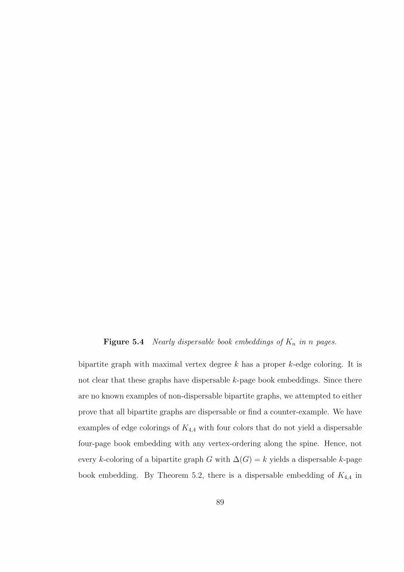
Figure 5.4 Nearly dispersable book embeddings of Kn in n pages.

bipartite graph with maximal vertex degree k has a proper k-edge coloring. It is

not clear that these graphs have dispersable k-page book embeddings. Since there

are no known examples of non-dispersable bipartite graphs, we attempted to either

prove that all bipartite graphs are dispersable or find a counter-example. We have

examples of edge colorings of K4,4 with four colors that do not yield a dispersable

four-page book embedding with any vertex-ordering along the spine. Hence, not

every k-coloring of a bipartite graph G with ∆(G) = k yields a dispersable k-page

book embedding. By Theorem 5.2, there is a dispersable embedding of K4,4 in

89

a 4-book. Although this graph is not a counter-example, it does show that we

cannot prove the result by taking an arbitrary k-edge coloring of a graph G with

∆(G) = k and find a corresponding dispersable k-page book embedding of G.

We have already shown that regular dispersable graphs are bipartite. But,

is the converse true? Are all regular bipartite graphs dispersable? Since there

are many possible edge-colorings of bipartite graphs and many possible vertex-

orderings, it is difficult to determine whether a particular graph is actually not

dispersable. We focus our attention on regular bipartite graphs because all bipar-

tite graphs are dispersable if all regular bipartite graphs are. This is true since

every bipartite graph with maximal vertex degree k is a subgraph of a regular

bipartite graph with maximal degree k.

We note that any k-regular subgraph of Kn,n has 2n vertices of degree k.

Hence, any dispersable k-page book embedding of such a graph must have n edges

on each of the k pages so that every vertex has degree one on every page of the

k-page embedding. It seems likely that for some regular subgraph of Kn,n this is

impossible. In an attempt to find one, we conducted a computer assisted search

which revealed that every regular subgraph of Kn,n (n ≤ 6) is dispersable. Beyond

n = 6, we are uncertain whether arbitrary k-regular subgraphs are dispersable.

However, for any n, there are certain values of k for which k-regular subgraphs of

Kn,n are dispersable.

All one-regular subgraphs of Kn,n are dispersable since these graphs consist

only of n disjoint edges that may be placed without crossing on a single page.

Similarly, two-regular subgraphs of Kn,n have dispersable two-page book embed-

dings. This is clear since such graphs consist of disjoint even cycles which each

have dispersable two-page book embeddings. Since Kn,n is dispersable, then the

only n-regular subgraph of Kn,n is dispersable. There is only one possible n − 1-

regular subgraph of Kn,n up to isomorphism. Since this is the subgraph formed

90

by removing any page of the dispersable n-page book embedding of Kn,n of Theo-

rem 5.2, it has the corresponding (n− 1)-page dispersable book embedding. From

here it is not clear how to proceed to find dispersable embeddings for k-regular

subgraphs of Kn,n when 3 ≤ k ≤ n− 2, so the question remains open.

The techniques of Theorem 5.1 are useful for finding book embeddings of the

Cartesian product of two graphs when one of the graphs is a dispersable bipartite

graph. What about the case when both graphs contain an odd cycle? In Theorem

5.1, to embed G×H in a book, we use the fact that H is bipartite to reverse the

vertex-orderings of adjacent copies of G. If H has an odd cycle, then the vertices of

H cannot be two-colored. Thus, the technique of reversing the vertex-ordering of

adjacent copies of G will result in two adjacent copies of G with the same vertex-

ordering. Each edge between two corresponding vertices in adjacent copies of G

with the same vertex-ordering must lie on its own page. Thus, if G has many

vertices, the number of pages required with this embedding scheme will grow as

the number of vertices of G grows. If we change the type of page, we can handle

odd cycles more efficiently.

Consider the Cartesian product of a graph G with book thickness bt(G) = k

and an odd cycle C2m+1. The odd cycle has ∆(C2m+1) = 2, but three colors are

required to color the edges of C2m+1. Similarly, three colors are needed to color the

vertices of C2m+1. So, C2m+1 is neither dispersable nor bipartite. If we alternate

the ordering of the vertices of G along the circuit C2m+1 as in Theorem 5.1, we

will need at least ‖V (G)‖ pages for the edges between the two adjacent copies of

G that have the same vertex-ordering. The next theorem shows how a book with

torus pages can reduce the number of pages needed.

Theorem 5.7 Let G be a graph with bt(G) = k and let m ≥ 1. Then

t(G× C2m+1) ≤ dk/2e+ 1.

91

Proof: Since G has a standard book embedding in k pages, then G is embeddable

in a dk/2e-page torus book using this k-page embedding. Hence, t(G) ≤ dk/2e.

Now place the vertices of C2m+1 along a torus spine. Replace each vertex of

C2m+1 with a copy of G, where the vertices of G are lined up corresponding to a

t(G)-page torus book embedding of G. Each copy of G is placed with the same

vertex-ordering. The edges joining corresponding vertices of G can all be placed

on a single torus page without crossing as shown in Figure 5.5.

Figure 5.5 Two-page torus book embedding of K4 × C5.

Now we see that t(G× C2m+1) ≤ t(G) + 1 ≤ dk/2e+ 1.

Theorem 5.7 could have been stated in terms of torus pages in the following

way.

Theorem 5.8 Let G be a graph with t(G) = k and let m ≥ 1. Then

t(G× C2m+1) ≤ k + 1.

Instead of one additional torus page for the edges between the copies of G, we

could have used two cylinder pages. For graphs G and H with multiple odd circuits,

general bounds for t(G ×H) and ct(G ×H) are not as easy to obtain. However,

both the torus book and the cylinder book appear to be better for handling such

92

graphs than the standard book. Again, as we have seen in the previous chapter,

minimizing the total number of pages needed to embed a certain graph can often

be simplified by using books with modified pages.

93

BIBLIOGRAPHY

[1 ] M. Aigner, Graph Theory: A Development from the 4-Color Problem, BCSAssociates, Moscow, Idaho (1987).

[2 ] F. Bernhart and P. C. Kainen, The Book Thickness of a Graph, Journal ofCombinatorial Theory, Series B 27 (1979) no. 3, 320–331.

[3 ] J. F. Buss, A. L. Rosenberg, and J. D. Knott, Vertex-Types in Book Embed-dings, SIAM Journal on Discrete Mathematics 2 (1989) no. 2, 156–175.

[4 ] J. F. Buss and P. W. Shor, On the Pagenumber of Planar Graphs, Proceedingsof the 16th Annual ACM Symposium on Theory of Computing (Washington,D.C., 1984), ACM , New York, 1984, 98–100.

[5 ] F. R. K. Chung, F. T. Leighton, and A. L. Rosenberg, Diogenes: A Methodol-ogy for Designing Fault-Tolerant VLSI Processor Arrays, Proceedings of the13th International Conference on Fault-Tolerant Computing (Milan, Italy,1983), IEEE, New York, 1983, 26–32.

[6 ] F. R. K. Chung, F. T. Leighton, and A. L. Rosenberg, Embedding Graphs inBooks: A Layout Problem with Applications to VLSI Design, SIAM Journalon Algebraic and Discrete Methods 8 (1987) no. 1, 33–58.

[7 ] R. A. Games, Optimal Book Embeddings of the FFT, Benes, and BarrelShifter Networks, Algorithmica 1 (1986), 233–250.

[8 ] M. R. Garey, D. S. Johnson, G. L. Miller, and C. H. Papadimitriou, TheComplexity of Coloring Circular Arcs and Chords, SIAM Journal on Alge-braic and Discrete Methods 1 (1980) no. 2, 216–227.

[9 ] F. Harary and G. Prins, The Number of Homeomorphically Irreducible Trees,and Other Species, Acta Mathematica, 101 (1959), 161.

[10 ] L. S. Heath, Embedding Outerplanar Graphs in Small Books, SIAM Journalon Algebraic and Discrete Methods 8 (1987) no. 2, 198–218.

[11 ] L. S. Heath, Embedding Planar Graphs in Seven Pages, Proceedings of the25th Annual IEEE Symposium of Foundations of Computer Science (SingerIsland, Florida, 1984), IEEE, New York, 1984, 74–83.

[12 ] L. S. Heath and S. Istrail, The Pagenumber of Genus g Graphs is O(g),Journal of the Association for Computing Machinery 39 (1992) no. 3, 479–501.

[13 ] D. A. Holton, B. Manvel, and B. D. McKay, Hamiltonian Cycles in Cubic 3-Connected Bipartite Planar Graphs, Journal of Combinatorial Theory, SeriesB 38 (1985), no. 3, 279-297.

[14 ] L. T. Q. Hung, A Planar Poset Which Requires Four Pages, Ars Combina-toria 35 (1993), 291–302.

[15 ] P. C. Kainen, personal communication.

[16 ] P. C. Kainen, The Book Thickness of a Graph II, Proceedings of the 20thSoutheastern International Conference on Combinatorics, Graph Theory,and Computing (Boca Raton, Florida, 1989), Congressus Numerantium 71(1990), 127–132.

[17 ] R. Kannan, Unraveling k-Page Graphs, Information and Control 66 (1985),1–5.

[18 ] K. S. Kedlaya, Outerplanar Partitions of Planar Graphs, Journal of Combi-natorial Theory, Series B 67 (1996) no. 2, 238-248.

[19 ] S. M. Malitz, Genus g Graphs Have Pagenumber O(√g), Proceedings of the

29th Annual IEEE Symposium on Foundations of Computer Science (WhitePlains, New York, 1988), IEEE, New York, 1988, 458–468.

[20 ] S. Moran and Y. Wolfsthal, One-Page Book Embeddings Under Vertex-Neighborhood Constraints, SIAM Journal on Discrete Mathematics 3 (1990)no. 3, 376–390.

[21 ] S. Moran and Y. Wolfsthal, Two-Page Book Embeddings of Trees UnderVertex-Neighborhood Constraints, Discrete Applied Mathematics 43 (1993)no. 3, 233–241.

[22 ] D. J. Muder, M. L. Weaver, and D. B. West, Pagenumber of CompleteBipartite Graphs, Journal of Graph Theory 12 (1988) no. 4, 469-489.

[23 ] B. Obrenic, Embedding DeBruijn and Shuffle-Exchange Graphs in Five Pages,SIAM Journal on Discrete Mathematics 6 (1993) no. 4, 642–654.

[24 ] L. T. Ollmann, On the Book Thickness of Various Graphs, Proceedingsof the 4th Southeastern Conference on Combinatorics, Graph Theory, andComputing, Utilitas Mathematica Publishing, Inc., Winnipeg, 1973, 459.

95

[25 ] A. L. Rosenberg, Book Embeddings and Wafer-Scale Integration, Proceedingsof the 17th Southeastern International Conference on Combinatorics, GraphTheory, and Computing (Boca Raton, Florida, 1986), Congressus Numeran-tium 54 1986, 217–224 .

[26 ] A. L. Rosenberg, The Diogenes Approach to Testable Fault-Tolerant Arrays ofProcessors, IEEE Transactions on Computers C-32 (1983) no. 10, 902–910.

[27 ] E. Stohr, A Trade-off between Page Number and Page Width of Book Em-beddings of Graphs, Information and Computation 79 (1988), 155–162.

[28 ] M. M. Syslo, Characterizations of Outerplanar Graphs, Discrete Mathematics26 (1979), 47–53.

[29 ] W. T. Tutte, A Theorem on Planar Graphs, Transactions of the AmericanMathematical Society 82 (1956), 99–116.

[30 ] J. H. Van Lint and R. M. Wilson, A Course in Combinatorics, CambridgeUniversity Press (1992).

[31 ] H. Whitney, A Theorem on Graphs, Annals of Mathematics 32 (1931), 378–390.

[32 ] M. Yannakakis, Four Pages are Necessary and Sufficient for Planar Graphs,Proceedings of the 18th Annual ACM Symposium on Theory of Computing(Berkley, California, 1986), ACM, New York, 1986, 104–108.

[33 ] M. Yannakakis, Linear and Book Embeddings of Graphs, VLSI Algorithmsand Architectures (Loutraki, 1986), 226–235, Lecture Notes in ComputerScience, Vol. 227, Springer, Berlin, 1986.

96