Dislocation-Based Finite Element Modelling of Elasto...

University of California

Los Angeles

Dislocation-Based Finite Element Modelling of

Elasto-plastic Material Deformation

A thesis submitted in partial satisfaction

of the requirements for the degree

Master of Science in Mechanical Engineering

by

James Jau-Kai Chiu

2004

c© Copyright by

James Jau-Kai Chiu

2004

The thesis of James Jau-Kai Chiu is approved.

J. S. Chen

Gregory Carman

Nasr M. Ghoniem, Committee Chair

University of California, Los Angeles

2004

ii

To my dear wife Joanne and my family for your everlasting support.

iii

Table of Contents

1 Introduction and Thesis Objectives . . . . . . . . . . . . . . . . . 1

1.1 An Introduction to Materials Modelling . . . . . . . . . . . . . . . 1

1.2 Significance of the Physical-based Materials Modelling . . . . . . 3

1.3 Thesis Objectives . . . . . . . . . . . . . . . . . . . . . . . . . . . 5

2 Previous Research . . . . . . . . . . . . . . . . . . . . . . . . . . . . 8

2.1 The Bergstrom Model . . . . . . . . . . . . . . . . . . . . . . . . 9

2.2 Kocks-Mecking Model . . . . . . . . . . . . . . . . . . . . . . . . 12

2.3 The Estrin Model . . . . . . . . . . . . . . . . . . . . . . . . . . . 14

2.4 The Gottstein Model . . . . . . . . . . . . . . . . . . . . . . . . . 18

2.5 Other Models . . . . . . . . . . . . . . . . . . . . . . . . . . . . . 21

3 Model Development . . . . . . . . . . . . . . . . . . . . . . . . . . . 22

3.1 Model Assumptions . . . . . . . . . . . . . . . . . . . . . . . . . . 23

3.2 Dislocation multiplication and immobilization . . . . . . . . . . . 24

3.3 Internal stress . . . . . . . . . . . . . . . . . . . . . . . . . . . . . 26

3.4 Dislocation velocity . . . . . . . . . . . . . . . . . . . . . . . . . . 27

3.5 Climb and Recovery . . . . . . . . . . . . . . . . . . . . . . . . . 28

3.6 Dynamic Recovery . . . . . . . . . . . . . . . . . . . . . . . . . . 31

3.7 Stability of subgrains . . . . . . . . . . . . . . . . . . . . . . . . . 32

3.8 Constitutive Relation . . . . . . . . . . . . . . . . . . . . . . . . . 33

3.9 Model Summary . . . . . . . . . . . . . . . . . . . . . . . . . . . 34

iv

4 Model Implementation . . . . . . . . . . . . . . . . . . . . . . . . . 36

4.1 Model Programming . . . . . . . . . . . . . . . . . . . . . . . . . 37

4.1.1 The Main Subroutine . . . . . . . . . . . . . . . . . . . . . 37

4.1.2 The Diffun Subroutine . . . . . . . . . . . . . . . . . . . . 39

4.1.3 The DLSODE Subroutine . . . . . . . . . . . . . . . . . . 41

4.1.4 Model Execution . . . . . . . . . . . . . . . . . . . . . . . 42

4.2 Model Calibration . . . . . . . . . . . . . . . . . . . . . . . . . . . 44

4.3 Finite Element Implementation . . . . . . . . . . . . . . . . . . . 45

4.3.1 Test Specimen Modelling and Meshing . . . . . . . . . . . 46

4.3.2 Material Property Definition . . . . . . . . . . . . . . . . . 47

4.3.3 Load Definition . . . . . . . . . . . . . . . . . . . . . . . . 50

4.3.4 Analysis Execution and Results . . . . . . . . . . . . . . . 50

5 Results and Experimental Model Validation . . . . . . . . . . . . 53

5.1 FORTRAN90 Implementation Results . . . . . . . . . . . . . . . 53

5.2 Finite Element Analysis Results . . . . . . . . . . . . . . . . . . . 58

5.3 Brief Analysis of Plastic Instability . . . . . . . . . . . . . . . . . 77

6 Conclusions . . . . . . . . . . . . . . . . . . . . . . . . . . . . . . . . 79

A Dislocation-based Constitutive Model FORTRAN90 Code . . . 83

B Sample Input File . . . . . . . . . . . . . . . . . . . . . . . . . . . . 96

C Sample Output File . . . . . . . . . . . . . . . . . . . . . . . . . . . 97

v

References . . . . . . . . . . . . . . . . . . . . . . . . . . . . . . . . . . . 100

vi

List of Figures

1.1 Multiscale Modelling Time and Space Constraints . . . . . . . . . 2

4.1 Flow Chart Algorithm of Main Subroutine . . . . . . . . . . . . . 38

4.2 Flow Chart Algorithm of Diffun Subroutine . . . . . . . . . . . . 40

4.3 True Stress Strain Curve Sample . . . . . . . . . . . . . . . . . . 43

4.4 Small Test Specimen Dimension . . . . . . . . . . . . . . . . . . . 46

4.5 Small Test Specimen 3D Model . . . . . . . . . . . . . . . . . . . 47

4.6 SOLID95 Element . . . . . . . . . . . . . . . . . . . . . . . . . . . 48

4.7 Model Meshing . . . . . . . . . . . . . . . . . . . . . . . . . . . . 49

4.8 Boundary Conditions . . . . . . . . . . . . . . . . . . . . . . . . . 51

4.9 Load Steps shown on engineering stress-strain curves . . . . . . . 52

5.1 HT-9 232C 0DPA true and experimental stress-strain curves . . . 54




5.5 F82H 232C 0DPA true and experimental stress-strain curves . . . 56




5.9 Typical Necked Sample . . . . . . . . . . . . . . . . . . . . . . . . 58

5.10 Typical Necked Sample Zoomed . . . . . . . . . . . . . . . . . . . 59

vii

5.11 Displacement Contour Plot . . . . . . . . . . . . . . . . . . . . . . 60

5.12 Uniaxial Stress Contour Plot . . . . . . . . . . . . . . . . . . . . . 61

5.13 HT-9 232C 0DPA . . . . . . . . . . . . . . . . . . . . . . . . . . . 62

5.14 HT-9 232C 0DPA Stage A . . . . . . . . . . . . . . . . . . . . . . 63

5.15 HT-9 232C 0DPA Stage B . . . . . . . . . . . . . . . . . . . . . . 63

5.16 HT-9 232C 0DPA Stage C . . . . . . . . . . . . . . . . . . . . . . 64

5.17 HT-9 232C 0DPA Stage D . . . . . . . . . . . . . . . . . . . . . . 64

5.18 HT-9 232C 0DPA Stage E . . . . . . . . . . . . . . . . . . . . . . 65

5.19 HT-9 232C 0DPA Stage F . . . . . . . . . . . . . . . . . . . . . . 65

5.20 HT-9 232C 0DPA stress-strain curves . . . . . . . . . . . . . . . . 67

5.21 HT-9 232C 0DPA Final Displacement . . . . . . . . . . . . . . . . 67







5.28 F82H 232C 0DPA stress-strain curves . . . . . . . . . . . . . . . . 71

5.29 F82H 232C 0DPA Final Displacement . . . . . . . . . . . . . . . . 71





viii



5.36 F82H 450C 0DPA Yield Drop . . . . . . . . . . . . . . . . . . . . 75



5.39 HT-9 232C 0DPA stress-strain curves with Mobile Dislocation . . 77



ix

List of Tables

4.1 HT-9 and F82H Constants . . . . . . . . . . . . . . . . . . . . . . 39

4.2 DLSODE Parameter Values . . . . . . . . . . . . . . . . . . . . . 41

4.3 Input Parameters and Typical Values . . . . . . . . . . . . . . . . 42

4.4 Output Parameters . . . . . . . . . . . . . . . . . . . . . . . . . . 42

4.5 Calibration Parameters . . . . . . . . . . . . . . . . . . . . . . . . 44

4.6 Calibration Parameters Values . . . . . . . . . . . . . . . . . . . . 45

4.7 ANSYS Input Material Properties . . . . . . . . . . . . . . . . . . 48

x

Acknowledgments

I want to thank Professor Ghoniem for his generous support and guidance, and

Dr. Sharafat and all members of the Computational Nano and Micromechanics

Lab for helping me and answering all my questions.

xi

Abstract of the Thesis

Dislocation-Based Finite Element Modelling of

Elasto-plastic Material Deformation

by

James Jau-Kai Chiu

Master of Science in Mechanical Engineering

University of California, Los Angeles, 2004

Professor Nasr M. Ghoniem, Chair

The main objective of this work is to develop a physically-based constitutive

model for plastic deformation within the framework of Finite Element Elasto-

plastic analysis. The Ghoniem-Matthews-Amodel dislocation-based creep model[47]

is extended to obtain local stress-strain relationships in the plastic regime. The

extended model is then applied to the martensitic steels, HT-9 and F82H at

various temperatures simulating constant strain rate tests to obtain local stress-

strain relations, specifically the true stress-strain curves. Finite Element Analysis

is then performed based on the developed constitutive stress-strain relationships,

and the engineering stress-strain curves are obtained. Results show that the

dislocation-based model can be calibrated against experiments using microstruc-

tural parameters. The engineering stress-strain curves obtained from Finite Ele-

ment Analysis via ANSYS are correlated with a wide range of experimental data,

showing the versatility of the model. It is proposed that such microstructure-

based, and experimentally-calibrated model can be confidently used in the pre-

diction of structural deformations under conditions not attainable experimentally

or of no experimental results available.

xii

CHAPTER 1

Introduction and Thesis Objectives

1.1 An Introduction to Materials Modelling

In the recent decades, due to the advancements in computing and electronic mi-

croscope technologies, a new realm of science of Materials Modelling has gained

much attention. Materials Modelling is a tool which is a set of computationally

programmed mathematical equations that are based on the micro to nano-scale

material parameters, such as dislocations and atoms. By inputting the desired

operating conditions of the material, such as temperature, stress, or strain rate,

material properties of interest such as true stress-strain relations and high tem-

perature creep curves can be readily predicted. This revolutionary concept is

however, still at its development stage. It is one of the objectives of this thesis

to implement a type of material model and exam its accuracy and applicability.

The objective of this chapter is to provide a brief introduction to the realm

of Materials Modelling, a brief introduction to one of the branches of Materials

Modelling-the Phenomenological-based Materials Modelling, and an introduction

to the overall project objectives.

Materials Modelling or Multiscale Modelling from Ghoniem et al[46] can be de-

scribed as an

analytical and computational ... framework to describe the mechanics

of materials on scales ranging from the atomistic, through the mi-

1

crostructure or transitional, and up to the continuum...

Multiscale Modelling or MMM can thus be traced back to the development of

Quantum Mechanics and Continuum Mechanics to the more recent frameworks

of Molecular Dynamics and Dislocation Dynamics. The necessity of modelling

materials with scales ranging from atomic to continuum is to be able to analyze

the mechanics of structures from nano to continuum scale. The demand to an-

alyze the structure at nano-scale has increased dramatically due to the recent

development in nanotechnology. The ability to integrate the analysis from nano

to continuum scale also posses high importance because MMM has promised to

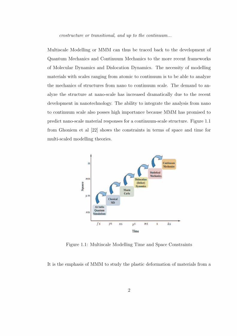
predict nano-scale material responses for a continuum-scale structure. Figure 1.1

from Ghoniem et al [22] shows the constraints in terms of space and time for

multi-scaled modelling theories.

Figure 1.1: Multiscale Modelling Time and Space Constraints

It is the emphasis of MMM to study the plastic deformation of materials from a

2

mechanics aspect. The importance of plastic deformation from Martinez[35] can

be summarized as the following:

• The limitation of experimental data on plastic deformations.

• The size contribution to material strength such as carbon-nanotubes.

• The inhomogeneity of deformation of structures.

One of the Materials Modelling Theory-The Phenomenological or Physical-based

Materials Modelling, is a theory that is on the Statistical Mechanics/Continuum

Mechanics scale. It is one of the objectives of this thesis to develop a Physical-

based Constitutive Model at this scale to study the plastic deformation of certain

metal alloys. The following section introduces the Physical-based Plastic Defor-

mation Modelling Theory.

1.2 Significance of the Physical-based Materials Modelling

The Physical-based Materials Modelling for plasticity is based on direct observa-

tion of physical phenomenons such as dislocation glide and micro-scaled material

parameters such as dislocation densities. Rest of this section will compare this

type of plasticity model with other types of plasticity models. There are a number

of types of plasticity models that ranged from atomistic to continuum as shown

on figure 1.1. The Experimental Model, such as the Johnson-Cook Model[37] is

on the continuum scale. The Physical-based Model is different from experimen-

tal plasticity models because the Physical-based Models should not have to be

parameter-fitted. The following is the experimental Johnson-Cook Model,

σ = Kεn (1.1)

3

where K and n are material parameters to be fitted for different temperatures

and materials. The Physical-based Models should be able to deduce local mate-

rial behaviors if all microstructure parameters have been calibrated correctly.

Another type of MMM theory is Crystal Plasticity. Crystal Plasticity is a Ma-

terials Model on the Statistical Mechanics Scale. Developed by Asaro and Rice

at 1977, this type of Materials Model treats each grain as a single crystal. The

Material deformations are formulated at the grain level for various slip systems.

The Macroscopic properties are obtained from averaging the behaviors from all

slip systems. The following Busso-McClintock Model[37] is a Crystal Plasticity

Model,

F p = aγama ⊗ naF p (1.2)

τal = |τ a| − sa µ(T )

µ0

(1.3)

γa = γ0exp− F0

kT〈1 − 〈 τa

l

τ0µ/µ0

〉p〉qsgn(τ a) (1.4)

where a is an individual slip system. The Physical-based Model is different from

Crystal Plasticity because the solid is considered as homogeneous for Physical-

based Model. Crystal Plasticity considers the solid as non-homogeneous.

Other MMM theories include Dislocation Dynamics, Molecular Dynamics, and

Quantum Mechanics which range from the Statistical Mechanics all the way to

the atomistic scales. Dislocation Dynamics, pioneered by Ghoniem et al[21] has

gained tremendous attention within the past decade. The Physical-based Mod-

elling is different from many of the atomistic models because it requires much

less computing resources and the materials are treated homogeneously.

The following summarizes the advantages and disadvantages of applying the

Physical-based Models.

Advantages:

4

• The Model captures the actual physical phenomenons.

• The Model can be solved relatively easy.

• It requires much less computing time.

Disadvantages:

• It is not as localized as the atomistic models.

• Certain physical assumptions still have to be made.

• Certain experimental calibrations are still required.

Even though the current research direction in the realm of Materials Modelling

is focused on Dislocation Dynamics, the long computing time of such method

still prevents it from being broadly used. The advantages of the Physical-based

Models of short computing time and its physical nature, makes it a competitive

tool of choice within the range of Multiscale Modelling Theories. The objectives

of this thesis will be outlined next.

1.3 Thesis Objectives

The overall objectives of this thesis can be stated as the following:

• Extension and modification of a previously developed model by Ghoniem

et al for time-dependent creep deformation to the case of elasto-plastic

deformations.

• Calibration of the extended model with the widest possible range of ex-

periments on two ferritic-martensitic steels. The calibration encompasses a

considerable range of temperatures and stresses.

5

• Correlation of the local stress-strain relationships (i.e., constitutive equa-

tion) to globally measured engineering stress-strain relationships via Finite

Element Modelling.

• Determination of the causes leading to plastic necking and instability in the

uniaxial tested specimen.

HT-9 and F82H are the two ferritic-martensitic alloys chosen to be studied. There

have been tremendous interests generated by nuclear scientists and engineers in

the past three decades in understanding the mechanical and microstructural be-

havior of certain low activation ferritic-martensitic alloys such as HT-9 and F82H.

These alloys can potentially be used to construct the core of fusion reactors due

to some of their unique physical properties.

The advantages that these ferritic-martensitic alloys posses include low nuclear

activation level after disposed, ability to withstand irradiation induced void swelling,

good compatibility with liquid metal coolants, and costs [58]. A wide range of

topics on these ferritic-martensitic alloys have been studied. Some of these topics

include tensile properties, irradiation induced hardening, ductile to brittle transi-

tion temperature, and creep. Both experimental and analytical works have been

done within these realms in order to gain better understanding of these alloys.

In recent decades, much emphasis has been placed on understanding the mi-

crostructure of materials and its relationship with the material macroscopic prop-

erties. One of the most important microstructure parameters of metal alloys is

dislocation.

Dislocations are material line defects that have been found to have strong cor-

relation with the yield strength and the inelastic deformation of metal alloys.

Much work have been done in recent decades to understand dislocations and its

interactions within the materials. The foundations of dislocation theories have

6

been pioneered by Read[64], Cottrell[11], Friedel[18], and Hirth[36] in the second

half of the twentieth century.

In the recent decade, dislocation theories have been formulated into various

Physical-based Models that could predict material properties at various condi-

tions. The dislocation-based creep model by Ghoniem, Matthews, and Amodeo[47]

was one of the models. Developed to study and predict creep behavior for ferritic-

martensitic alloys mentioned earlier, this model has proven to be successful. It is

now one of the objectives of this present thesis to extend the Ghoniem-Matthrews-

Amodeo Creep Model into a Constitutive Model to study the stress-strain be-

haviors of these alloys in the plastic regime.

A number of Physical-based Models based on dislocation theories will be pre-

sented in the following chapter. Chapter 3 will outline and discuss the formu-

lations of the dislocation based Physical Model developed by Ghoniem et al.

Chapter 5 lists and discusses the findings from executing the developed Consti-

tutive Model, and Chapter 6 discusses the conclusions derived from executing the

model and examining the results.

7

CHAPTER 2

Previous Research

In this chapter, a number of dislocation density based materials models will be

reviewed and compared. Again, the reasons for formulating materials models

based on dislocations is to accurately capture the physical behaviors of materials

at a micro-scale as the previous chapter had mentioned. The applications of such

models can be used in either creep or constitutive predictions as one would see

in this chapter.

The development of physical or dislocation based materials models can be traced

back to the 1950’s. Some of the earliest scientists and metallurgists were working

to explain the work-hardening or softening behaviors of various FCC or BCC met-

als, specifically on the stage II hardening of FCC metal crystals. It was generally

concluded by many through experimental studies and theoretical formulations

that a flow stress model for a metal crystal can be formulated by a unique rela-

tionship correlating the flow stress and the square root of the dislocation density,

and an evolutionary equation of the dislocation density. However, there were no

consensus on how exactly the stress-dislocation equation should be formed, and

how to describe the complex dislocation evolutionary phenomenon.

Some of the earliest works to formulate the dislocation evolutionary phenomenon

include those by Seeger et al[4] on dislocation pile-ups, and Basinski[6] on for-

est dislocations. Some of the earliest comprehensive models were formed by

Kocks[38], Bergstrom et al[7][61], and later by Mecking and Kocks[31] which

8

was the milestone K-M Model. The first comprehensive model, the Bergstrom

model[7] will be discussed first.

2.1 The Bergstrom Model

The Bergstrom model was intended to predict homogeneous deformation, the

deformation from the onset of plastic deformation until the onset of necking for

BCC α-Fe at room temperature. One can begin to summarize the model by the

following,

σ = σi + σ∗ + σd (2.1)

where σi is the athermal strain independent stress, σ∗ is the strain rate and dislo-

cation dependent thermal stress, and σd is the long-range interaction dependent

term. σ∗ and σd are expressed as the following,

σ∗ = σu|ε

ΦbL|1/m∗

(2.2)

σd = αGb√

ρ (2.3)

where ε = ΦbLv. Φ is an orientation factor(0.5 for polycrystalline), b is the

Burgers vector, L is the density of mobile dislocations, and v is the average

velocity of the mobile dislocations. v can be calculated as v = | σ∗

σu

|m∗, where

σ∗ is the effective stress acting on a dislocation, σu is the effective stress giving

the dislocation an average unit velocity, and m∗ is the temperature-dependent

material constant. From 2.2 and 2.3, 2.1 can be then expressed as

σ = σi + σu|ε

ΦbL|1/m∗

+ αGb√

ρ (2.4)

The evolutionary rate equation for the immobilized dislocations ρi can be ex-

pressed as the followingdρi

dε= U − dr

dε− da

dε(2.5)

9

where U is the rate at which the mobile dislocation dislocations is increased

by creation and or re-mobilization processes, drdε

is the rate at which immobilized

dislocations are re-mobilized, and dadε

is the annihilation rate. It has been assumed

that the mobile dislocation density is much smaller than the total dislocation

density, thus the total dislocation density ρ can be approximately as the immobile

dislocation density ρi. U can be calculated as inversely proportional to the mean

free path of the mobile dislocation as the following.

U(t) =vL

s(t)(2.6)

The term drdε

, the rate at which immobilized dislocations are re-mobilized can be

simply written as the following

dr

dε= θ1ρi (2.7)

where θ1 is a material constant independent of strain, and ρi is the immobile

dislocation density. The annihilation term da/dε is divided into three processes

by Bergstrom. They are mobile dislocation annihilating each other, mobile and

immobile dislocations annihilate each other, and mobile dislocation annihilating

with microstructure surfaces such as grain boundaries. It has been postulated by

Bergstrom that the mobile dislocations annihilation rate is proportional to the

square of the mobile dislocation density. The immobile and mobile dislocation

annihilation rate is proportional to the product of mobile and immobile disloca-

tion densities, and the mobile to surface annihilation rate is proportional to the

product of the strain independent annihilation space L and the mobile dislocation

density. da/dε can then be expressed as the following

da

dε= λ1L

2 + λsLρi + θNL (2.8)

where λ1, λ2, and θ2 are strain independent constants. From 2.6, 2.7, and 2.8,

2.5 can be written as the following, assuming that the mobile dislocation is time

10

independent.

dρi

dε= U(ε) − θ1ρi − λ1L

2 − λ2Lρi − θ2NL ' dρ

dε= U(ε) − A − Ωρ (2.9)

A = (λ1 − λ2)L2 + (θ2N − θ1)L (2.10)

Ω = θ1 + λ2L (2.11)

If U , the rate of immobilization and annihilation of mobile dislocations are as-

sumed to be strain independent, and Ω, the probability of re-mobilization and

annihilation between immobile and mobile dislocations is assumed to be small,

then the following stress strain relation can be attained.

σ = σi0 + αGbU − A

Ω(1 − e−Ωε) + ρ0e

−Ωε1/2 (2.12)

σi0 = σi + σu[ε

ΦbL]1/m∗

(2.13)

The above model has been extended to predict behaviors of FCC polycrystallines

from [61]. From [61] 2.6 can be expressed as the following,

U(ε) =1

100θbs(ε)(2.14)

where θ is an orientation factor about 0.5 for BCC and 0.32 for FCC. For FCC,

due to fewer slip systems and limited cross slip, the dislocation evolutionary

equation can be modified to be the following,

dρ

dε=

1

100θb[s0 + (s1 − s0)e−kε]− Ωρ (2.15)

where s is the mean free path of mobile dislocation. s0 is an equilibrium value,

and s1 is the initial condition of s at ε = 0. If Ω = 0, then the stress strain

relation can be revised to be the following,

σ = σi0 + αGbρ0 + U0ε +U0

kln(

s0 + (s1 − s0)e−kε

s1

)1/2 (2.16)

11

where ρ0 = ρ at ε = 0 and U0 = 1/100θbs0 = 1/bs0. [7] and [61] are limited

to uniaxial strain with homogeneous deformation under ambient temperatures.

Modified model by Bergstrom et al have taken higher temperature deformations

into consideration[65]. It was proposed by Bergstrom from experimental stud-

ies that the recovery parameter Ω should be separated into an athermal and a

thermal term as the following.

Ω = Ω0 + Ω(ε, T ) (2.17)

From some of the well studied assumptions regarding recovery that the thermal

term of recovery is due to vacancy and interstitial diffusions of dislocations with

subgrain walls. Incorporating the assumptions in [65], the thermal recovery term

can be written as the following,

Ω(ε, T ) = kn0(2D0)1/22/3exp(− Qm

3RT)ε−1/3 (2.18)

where k and D0 are constants. n0 is the number of vacancies per unit volume,

and Qm is the vacancy migration energy. The validity of the above model has

been shown in [7], [61], and [65] to correlate quite well with experimental results.

Despite its well organized dislocation evolutionary equation(3 parameters, U , A,

and Ω), its treatment on the contribution of various types of dislocations (mobile,

immobile) would be further advanced by other models[47].

2.2 Kocks-Mecking Model

Kocks and Mecking[31] formulated a similar model and is now known as the

Kocks-Mecking (KM) model. This model will be discussed next. The KM model

is similar to the Bergstrom model because it utilizes the square root of the dis-

location density relation with the flow stress. Therefore, the following kinetic

12

equations were proposed,

σ = αµb√

ρ (2.19)

σ = s(ε, T )σ (2.20)

where σ is a reference flow stress at a reference temperature, and α is a constant

depending on the dislocation interactions. The flow stress at a finite temperature

is described by 2.20 as the product of s and the reference stress σ. If other

resistance such as lattice resistance, solution hardening, and grain size effects are

taken into consideration, then 2.20 can be extended to be

σ = α(ε, T )µb√

ρ + σ0(εT ) (2.21)

The evolutionary equation is expressed as the rate between the dislocation storage

and dynamic recovery as the following,

dρ

dε=

1

Λb− LrNr

vr

ε(2.22)

where Λ is the mean free path. Lr is the dislocation length. Nr is the number of

dislocation per unit volume, and vr is the rate of recovery. The reference stress

σ and the flow stress σ is correlated by the following,

s(ε, T ) ≡ σ

σ= (

ε

ε0

)1/m (2.23)

where m is a temperature dependent constant. It has been pointed out by Kocks

and Mecking that 2.23 is not sufficient to describe dynamic recovery and the

”transient” behavior. Therefore, 2.23 can be modified as the following to accom-

modate dynamic recovery,

s = (ε

ε0

)1/mexp(−Fθr

θh

) (2.24)

s = (ε

ε0

)1/m(1 − Fθr

θh

) (2.25)

13

where θh is the athermal hardening rate and θr is the recovery rate. This one

parameter model has been found to work quite well under continuous deforma-

tion such as constant strain rate or stress[15], and its formulation is simple and

elegant. The work of Estrin et al[15], [16], [66] has extended the KM model to

predict material deformation for more complicated loading scenarios, which will

be discussed next.

2.3 The Estrin Model

From the work by Estrin et al[15], 2.22 can be re-written as

dρ/dε = k1ρ1/2 − k2ρ (2.26)

where k1 and k2 are constants. From 2.19 and 2.26, that the following evolution

equation can be written,

dσ/dε = θ0(1 − σ/σs) (2.27)

where

θ0 = αGbk1/2 (2.28)

σs = αGb(k1/k2) (2.29)

From [15], the kinetic equation that relates the flow stress and the hardness

parameter σ can be shown to be

σ/σ = (ε/ˆε)1/m (2.30)

where m is a temperature dependent constant. Equations 2.27, 2.28, 2.29, and

2.30 constitutes the Estrin Model, which is very similar to the KM Model. Estrin

et al have proposed a modified version of the above model[66] [16], and it will be

14

presented in the following paragraphs. One can begin the modified Estrin Model

with the Levy-von Mises equation

˙εijp =

3

2

εp

σsij (2.31)

˙εij = ˙εije + ˙εij

p (2.32)

where

εp =

√

2

3˙εij

p ˙εijp = ε0(

σ

σ)m (2.33)

σ =

√

3

2sijsij = σ(

εp

ε0

)1/m (2.34)

The structure parameter σ can be expressed as the function of dislocation density

ρ as the following,

σ = MαGb√

ρ (2.35)

where M is the average Taylor factor. The evolution equation is the following,

dρ/dεp = k1

√ρ − k2ρ (2.36)

where the constant k1 is associated with dislocation storage, and the constant

k2 is associated with dislocation annihilation by recovery. The strain rate and

temperature dependent constant k2 can be obtained by the following,

k2 = k20(εp

ε∗0)−1/m (2.37)

where k20 is a constant. n and ε0∗ are temperature dependent constants. If

constant plastic strain rate is assumed, then equations 2.33 to 2.37 can be solved.

The following is the stress-strain relation,

σ − σs

σi − σs

= exp(−εp − εpi

εtr

) (2.38)

15

where

σs = MαGbk1

k20

(εp

ε0

)1/m(εp

ε∗0)1/n (2.39)

εtr = σs/ΘII (2.40)

ΘII =1

2M2αGbk1(

εp

ε∗0)1/m (2.41)

If forming process such as hot forming, which the phenomenon of static recovery

due to dislocation climb must be included, 2.36 can be modified as the following,

dρ/dεp = k1

√ρ − k2ρ − r/εp (2.42)

where

r = r0exp(− U0

kBT) sinh

β√

ρ

kBT(2.43)

r0 is a constant, U0 is the activation energy, β is constant, and kB is the Boltzmann

constant. The above model has been shown by Estrin et al to match experimental

results quite well. However, if simulating non-monotonic deformation is necessary,

then the ”one-parameter” model such as the Estrin and the KM model would

not be sufficient. The following model[66] proposed by Estrin et al tackles the

case of cyclic deformation. The ”two-parameter” model by Estrin et al for a

monotonic loading case begins with the following kinetic equation between the

inelastic strain εin and the applied stress σ.

εin = ξ |σ|σ0

√YmXsign(σ) (2.44)

X and Y are internal variables and defined as

X(t) =ρm(t)

ρm(0)(2.45)

Y (t) =ρf (t)

ρf (0)(2.46)

where ρm is the mobile dislocation density and ρf is the immobile or forest dis-

location density at time t. The evolutionary equations for the internal variables

16

X and Y with respect to the inelastic strain are defined as the following,

∂X

∂|εin| = [−C − C1

√Y − C3X + C4

Y

X]q (2.47)

∂Y

∂|εin| = C + C1

√Y − C2Y + C3X (2.48)

where q is ρf (0)/ρm(0). The coefficients C to C4 all bear physical significance

such as C, which models the effect of nonshearable second-phase particles or

grain boundaries. For details, see [66]. For a cyclic loading case, an additional

internal variable Z must be introduced to account for recoverable dislocations

that trapped at the subgrain walls, ρri. The additional evolutionary equations

due to Z is the following.

∂Z

∂t= (C5

√Y − C2Z)εp − C6Z (2.49)

where Z = ρri(t)/ρri(0). The evolutionary equation for X, equation 2.47 would

have to be modified to be

∂X

∂t= (−C − C1

√Y − C3 + C4

Y

X+ C∗

7Z)q|εin| (2.50)

where C∗7 = C7 for |σ| < σ0

√Y , 0 otherwise. The kinetic equation 2.44 must

be modified and an additional back stress σback must also be introduced as the

following.

∂σback

∂εin= C8

√Y sign(ε)in − C9σback (2.51)

εin = ξ|σ| − |σback|σ0

√Y

msign(σ − σback) (2.52)

The above cyclic loading model has been found to match experimental results

quite well. For experimental details, see [66]. Gottstein et al[27][20] have pro-

posed other multi-parameter dislocation based models. The Gottstein models

will be outlined in the following section.

17

2.4 The Gottstein Model

The Gottstein Model was proposed by Gottstein et al[27] at 1987 to study and

predict metallurgical behaviors under creep(constant stress) and constant strain

rate testings. The derivation of the model begins with the following assumption

of dislocations.

dρ = dρ+ +∑

i

dρ−i (2.53)

dρ+ is the dislocation production and dρ−i denotes the contribution of various

recovery mechanisms. The strain increment is represented as

dε = dεDIS + dεSUB (2.54)

where dεDIS is glide of mobile dislocation and dεSUB is the collective subgrain

dislocation movements. The production rate dρ+ can be represented as

dρ+ = dεDIS/bL (2.55)

where L the slip length is inversely proportional to the mean free path as L =

κ/√

ρ. The subgrain movement dεSUB is the following,

dεSUB = ρSUBbvSUBdε

ε(2.56)

where ρSUB is the subgrain dislocation density. From 2.54 to 2.56, the production

rate with subgrain movement can be obtained as.

dρ+ = dε(

√ρ

bκ− 1

εκρSUBvSUB

√ρ) (2.57)

Provided that ρSUB = βρ, the average subgrain size d = λ√

ρ, the subgrain velocity

vSUB = mλβbγσ, and the recovery process as the following,

ρ− = dρ−GLIDE + dρ−

CLIMB + dρ−SUB (2.58)

18

where

dρ−GLIDE = −LR

bρdε (2.59)

dρ−CLIMB = −Dc

χρ2dt = −Dc

χρ2dε

ε(2.60)

dρ−SUB = −ρSUBvSUB

d

dε

ε(2.61)

LR is the swept-up line length per recovery site, and Dc is the diffusion con-

stant for the climb process. The evolutionary equation according to can then be

expressed as the following,

dρ = dε√

ρ

bκ− LR

bρ − (

Dc

χ+ Mσ[1 +

λ

κ])

ρ2

ε (2.62)

where M = mβ2b. For the case of constant strain rate test, the flow stress is

related to dislocation density by the common equation.

τ = αµb√

ρ (2.63)

From 2.62 and 2.63, the hardening coefficient θ can be obtained as.

θ ≡ dτ

dε=

αµ

2κ− LR

2bτ − (

Dc

χ+ Mσ[1 +

λ

κ])

τ 3

2(αµb)

1

ε(2.64)

For the case of a creep test, the following strain rate expression can be derived.

ε =Φ√ρ

+ Mλbσρ3/2 =1√ρ(Φ + Mλbσρ2) (2.65)

The steady state stress, transient creep, steady state creep can then be studied by

the above model. The three-parameter model was further modified by Gottstain

et al[20] to account for more physical phenomenons such as precipitate hardening

and to account for multiple slip systems by introducing the Taylor factor. The

external stress can be found by the following relation,

σext = M(fiτi + fwτw) (2.66)

19

where M is the Taylor factor. fi, τi and fw, τw are volume fractions and resolved

shear stress of subgrain(cell) interior and wall. The effective shear stress is related

to the dislocation density as the following.

τx = τeffx+ αGb

√ρx, x = i, w (2.67)

The following kinetic equation, the Orowan equation, is used to solve for the

effective shear stress under constant strain rate,

γ = εM = ρmbv (2.68)

where γ is the shear strain rate, and v is the glide velocity as given by the

following.

v = λv0exp(− Q

kBT) sinh(

τeffV

kBT) (2.69)

λ is the jump width-the mean spacing of obstacles, v0 is the attack frequency,

Q is the effective activation energy for glide, and V is the activation volume.

The evolutionary equations for the three parameters can be summarized as the

following,

˙ρm = ˙ρm+ − ˙ρm

−,lock − ˙ρm−,anni − ˙ρm

−,dip =εM

bLeff

−

4dlockεM

b

n − 1

nρm − 2danni−c

εM

b

1

nρm − 2(ddip − danni−c)

εM

b

1

nρm (2.70)

ρi = ρi+ − ρi

− = ˙ρm−,lock − 2danni−gvclimb

1

nρ2

i (2.71)

ρw = ρw+ =

1

fw

˙ρm−,dip (2.72)

Please see [20] for details of the parameters in the above equations. The model

summarized above has been shown to be able to predict the mechanical material

behavior quite well for two-phase aluminium alloys at elevated temperatures, and

has been interfaced with Finite Element Analysis for crystal plasticity. There are

many other models that are based on subgrain structures and multi-parameters.

The following section will briefly highlight these other models.

20

2.5 Other Models

Some of the other models and microstructure formulations include ones by Lagneborg

et al[51], which is based on formulating a dislocation distribution frequency func-

tion Φ(l). The evolutionary equations are then formulated by integrating the

frequency function. The model by Prinz et al[19] was formulated based upon

a plastic resistance τ to glide. Once the plastic resistance is solved, the plastic

strain can then be solved. Blum et al[63][62][44][52], further investigated the non-

monotonic loading conditions for creep, and has deduced a number of models,

specifically basing on the composite model developed by Mughrabi et al[42][43],

to explain various mechanisms such as glide and recovery. Similar works have

also been done by Argon et al[5] and Zehetbauer[68] on FCC Metals. The works

by Nabarro[45] on diffusional creep and the works by Gittus[26][23] on disloca-

tion creep have also laid great foundations for the recent works in the area of

dislocation based materials modelling.

21

CHAPTER 3

Model Development

The dislocation based constitutive model is based on the dislocation creep model

developed by Ghoniem et al[47]. The dislocation based creep model was ini-

tially developed to predict high temperature deformation under arbitrary time-

dependent stress and temperature histories for engineering materials in harsh

environments. One of the applications of the creep model is to predict creep for

ferritic alloys such as HT-9 and F82H. These alloys have been considered as the

materials for the core of nuclear fusion reactors due to their low activation na-

ture and good ability to withstand irradiation induced void swelling. HT-9 and

F82H will also be the materials investigated by this dislocation based constitutive

model as previously stated.

The dislocation creep model is a comprehensive model based on a compilation of

developments in creep theory from recent decades such as the work by Nabarro[45]

and Gittus[26] which were previously mentioned, and such as the works by Bul-

lough et al[50] on rate theory. The objective of developing this dislocation based

constitutive model is to be able to apply this model to Finite Element Analysis,

and to study mechanical material behaviors for the alloys mentioned above. The

studying of the ability to model the Mechanical behaviors of strain softening is

also another subject of interest. Works by Heald et al[28] and Bullough et al[8]

on irradiation creep mentioned in [47] are also possible directions of future inves-

tigations via this model. The inclusion of subgrain microstructure evolution is a

22

key aspect of this model. The processes of subgrain evolution has been reviewed

by Holt[29] as mentioned by Ghoniem et al[47]. The details of the development of

the dislocation based constitutive model will be explained in the following. This

dislocation based constitutive model is composed of six rate equations to predict

the behavior of six engineering parameters, namely the creep strain, the mobile,

static and boundary dislocation density, the subgrain radius, and the applied

stress.

3.1 Model Assumptions

A number of references(Takeuchi et al[56], Langdon[39], Challenger et al[9],

Michel et al[13], and Cuddy[12]) on the investigations of subgrain and high tem-

perature alloy characteristics were summarized by Ghoniem et al [47]. This paper

will briefly re-summarize these characteristics and assumptions as a point of de-

parture to develop the dislocation based constitutive model. The following can

be stated about alloys operating at high temperatures.

• Dislocation pileups and debris due to cold works are not observed

• Dislocation form a polygonal network called subgrains, and they nucleate

at high enough temperatures

• The applied stress is inversely proportional to the dimension of the sub-

grains

• The dislocation density within the subgrains are low, and increases with

the square of the applied stress

• The formation of subgrains may be delayed to higher temperatures in ma-

terials with lower stacking fault energy

23

• Subgrain growth may be inhibited by solute-hardened alloys

• Subgrains are commonly seen in materials with low stacking fault energy,

extensive precipitation, and substantial concentration of hardening solutes

The various dislocation processes discussed by Gittus[23], Li[40], and Sandstrom[54][53]

can be summarized as the following.

• Multiplications of dislocations within the subgrains

• Annihilation of mobile dislocations within the subgrains

• Annihilation of dislocations at the subgrain walls

• Absorbtion of dislocations by the subgrain walls

• Emissions of dislocations by the subgrain walls

• Nucleation of new subgrains

• Growth of subgrains by coalescence

These phenomenons described above were modelled by Ghoniem et al[47] to study

dislocation creep. It is the objective of this paper to study constant strain rate

(CSR) test based on the original model.

3.2 Dislocation multiplication and immobilization

The model is commenced by the Orowan equation as the following, which is used

as the kinetic equation for this dislocation based constitutive model.

dεp/dt = bρmvg (3.1)

24

εp is the creep or plastic strain. ρm is the mobile dislocation density, which is the

dislocation density within the moving dislocation density within the subgrain. vg

is the glide velocity, and b is the Burger’s vector. The glide process is assumed to

be easy, and the effect the climb is ignored. Since this is a uniaxial model, only

one slip system is considered. Therefore the value of b, the burger’s vector can

be obtained from empirical references. However, the instantaneous value of the

mobile dislocation density and glide velocity would have to be formulated.

It is understood that the subgrains provide a source and also act as barriers for

mobile dislocations. In order to form a rate equation for dislocation, the rate of

dislocation production and annihilation must be formulated. From [47], the rate

of the mobile dislocation is produced within the subgrains is formulated as the

frequency of the dislocation produced multiplied by the number of dislocation

produced. It can shown as the following.

˙ρm = ρ3/2m vg (3.2)

The frequency of production is ρ1/2m vg, where ρ1/2

m is the reciprocal of the mean

free path of the mobile dislocations. The effects of subgrain wall and subgrain

radius would also have to be considered. The potential density of source can be

characterized as 1

2h2Rsb, where h is the dislocation spacing within the subgrains,

and Rsb is the subgrain radius. The dislocation spacing within the wall, h can be

formulated as the following, where ρs and ρb are static and boundary dislocations.

h = 1/(ρs + ρb)Rsb (3.3)

From the above, two rate equations can be formulated as the following.

˙ρm = βρsRsbvg/h2 − ρmvg/2Rsb (3.4)

ρs = ρmvg/2Rsb (3.5)

25

where β is a density factor. It is apparent that the immobilization term of

equation 3.4 is equation 3.5.

3.3 Internal stress

The internal stress must be analyzed since the effective stress, which is a function

of internal stress, will be incorporated in the formulation of dislocation velocity.

Again, from [47], the internal stress is caused by any opposition to dislocation

motions, and this opposition can be characterized into three sources. The first

source is any precipitates and other dislocations that oppose dislocation motions.

The internal stress that mobile dislocations must overcome is µb/2πλ, where λ is

the effective obstacle spacing, and µ is the shear modulus. In the case where both

precipitate and dislocation obstacles are present, the effective obstacle spacing λ

is given as the following.

λ = 1/(1/λd + 1/λp) (3.6)

λd is the inter-dislocation spacing, and is given as λd = 1/ρ1/2m . λp is the inter-

precipitate spacing, and is given as λp = 1/(Nprp)1/2, where Np is the volume

concentration of precipitates, and rp is the mean radius.

The second source of opposition are the dislocations that have not yet neutralized

their long range stress fields. Essentially these dislocations have not moved into

their low energy configuration. The mobile dislocations could be accelerated or

retarded depending on the nature of these un-neutralized stress fields. These

unstable dislocations are static dislocations within the subgrains. The boundary

dislocations themselves do not contribute to the internal stress beyond a distance

greater than the average dislocation distance within the subgrains[18]. Combining

the effects of precipitates and unstable static dislocations. The long range internal

26

stress can be expressed as the following.

σi = µb/2πλ + ζµbρ1/2s (3.7)

The third source of opposition is the friction resistance to glide from over-sized

solutes. These typically are solute particles used to strengthen metals. From [47],

for well-annealed materials without hardening precipitates and heat treatment,

this stress can be identified as the initial flow stress, σ0. Therefore, the effective

stress, σe can be represented as the following, where σa is the applied stress.

σe = σa − σi − σ0 (3.8)

3.4 Dislocation velocity

From[47], the dislocation velocity does not contribute significantly to the steady

state creep strain rate. However, the dislocation velocity does affect the tran-

sient creep strain rate, and its relationship with stress, dislocation density affects

the long term strain rate as well. The formulation of dislocation velocity can

primarily be dictated by the effect of solute atoms. The following formulation

given by[57][10], accounts for the viscous nature of dislocation movement under

low stress

vg = DakTbσe/[c0(β∗)ln(R/r)] (3.9)

where σe is the effective stress, c0 is the uniform volume concentration of the

solute, Da is the solute diffusion coefficient, R is the outer cutoff radius, and r is

the inner cutoff radius. The value of β∗ is given by [36]

β∗ = (µb/3π)[(1 + ν)/(1 − ν)](vs − va) (3.10)

where ν is the Poisson’s ration, vs is the solute atomic volume, and va is the matrix

atomic volume. When solute atoms are trapped at the core of the dislocations,

27

the following equation can be formulated[36]

vg ≈ 2bvdexp(−2a/kT )sinh(σeb2la/kT ) (3.11)

where vd is the dislocation vibrational frequency, Wa is the activation free energy

for core diffusion of the solute, and la is the spacing of the solute atoms in the

core. Another empirical formulation for the dislocation velocity is the following.

vg = a1exp(−Wg/kT )σeΩ/kT (3.12)

where a1 and Wg are parameters to be fitted, and Ω is the atomic volume. If the

effect of cutting of the obstacle is considered, the following can be formulated.

vg = vdλsinh(σeb2λ/2kT )exp(−Ug/kT ) (3.13)

Ug is the activation energy for the process, which is approximately twice the jog

formation energy.

3.5 Climb and Recovery

The phenomenon of dislocation climb contributes to the recovery of dislocations

over time. The effect of climb recovery is considered to be the climb of dislocation

dipoles into the subgrains. The effective stress the dislocation dipoles exert on

each other can be expressed as the following, where s is the separation distance

between the dipoles.

σc = µb/2π(1 − ν)s (3.14)

The vacancy concentration near the dislocations ccvd will be enhanced or reduced

depending on the vacancy interaction. If the thermal equilibrium concentration

is ccv, then cc

vd can be expressed as the following.

ccvd = ccexp(±σcΩ

kT) ' cc(1 ± σcΩ

kT) (3.15)

28

The net flow of vacancies into dislocations can be expresses as the following rate

equation under irradiation.

dqd

dt= k2

idDici − k2vdDvcv + k2

vdDvcvd (3.16)

k2id, Di, and ci are the dislocation sink strength for interstitial, interstitial dif-

fusion coefficient, and the interstitial bulk concentration. k2vd, Dv, and cv are

equivalent parameters for vacancies. The interstitial and vacancy concentration

can be expressed by the following rate equations

∂ci

∂t= K + k2

i Dici − αcicv (3.17)

∂cv

∂t= K + k2

vDvcv − αcicv (3.18)

where K is the rate of production of Frenkel pais, k2i and k2

v are the sum of the

sink strength from all the potential sinks for interstitial and vacancies, Kve is

the sum of the vacancy emission rates for all the sinks, α is the rate constant for

interstitial and vacancies. The sink strength, according to Rauh and Bulllogh[49],

can be expressed as

k2αN = − πρN

ln[(1/2)eγ(kαLα)]' − 2πρN

ln(kαLα)(3.19)

where the subscript α refers to either interstitial or vacancy, N refers to network

dislocations, and γ is Euler’s constant, ∼ 0.5772. La is a length parameter that

governs the range of interactions between dislocations and defects.

Lα = (1 + ν)µb|4Vα|/3π(1 − ν)kT (3.20)

4Vα is the relaxation volume of the defect, and it is typically −0.5Ω for vacancy

and 1.2Ω for interstitial. The difference between vacancies and interstitial has

been considered as the cause for irradiation induced swelling. If the dislocation

network is the only sink for vacancies, then 3.19 can be approximated as

k2αN = −2πρN/ln(ρ

1/2

N Lα) (3.21)

29

The transfer of defects into jobs on the dislocation is controlled by the following

ηα = cjb(aαcvαc)exp(−4Wα/kT ) (3.22)

where cj is the job concentration, aαc and aα are the geometric factors, vαc and

vc are the attempt frequency for jumps, and 4Wα is the difference in activation

energy. Argon and Moffatt[2] have proposed a revised 3.22 to be the following

ηα = 103fαcjb(Γ/µb)2 (3.23)

where γ is the stacking fault energy. Taking transfer rate into consideration, 3.19

becomes the following.

k2αd = 2πηαρN/[1 − ηαln(ρ

1/2

N Lα)] (3.24)

Since dislocation dipoles are the primary interest, the sink strength for dipoles

according to Hirth[36] becomes

k2αd = 2πηαρN/[1 − ηαln(k2

αLαs)] (3.25)

where s is the dipole separation distance. Assuming no irradiation effect, then

3.16 reduces todqd

dt= k2

vdDsσcΩ/kT (3.26)

where the lattice self-diffusion coefficient Ds = Dvcev. The climb velocity is

vc = (dqd/dt)/bρd (3.27)

From 3.14, 3.25, 3.26, and 3.27, the dipole separation can be expressed as

ds/dt = −2ηDsµΩ/(1 − ν)skT [1 − ηln(k2αLαs)] (3.28)

3.28 can be integrated with initial dipole separation s0 to be the following.

τ = −(1 − ν)kT

4DsµΩs20[ηvln(k2

vLvs) −ηv

2− 1] ' s0

4vc

(3.29)

30

The mobile dislocation recovery rate can be expressed as the following, assuming

all dislocations are part of the recovery process, and the initial dipole separation

is s0 = ρ−1/2m .

˙ρm = −2ρm

τ= −8ρ3/2

m vcm (3.30)

The static dislocation recovery can be expressed as the following, assuming that

the initial dipole separation is s0 = h and k2v = 1/h2.

ρs = −2ρs

τ= −8ρs

vcs

h(3.31)

A possibility of diffusion short-circuited by the dislocation core has been inves-

tigated by Evans et al[17]. The flux of vacancies along the dislocation can be

expressed as.

jp = 2ηvDpσeΩ/(b + ηvLp)kT (3.32)

where ηv is the transfer coefficient of vacancies from dislocation to jobs. Dp is

the core diffusion coefficient, and Lp is the path length for diffusion along core. If

jog spacing is much less than the diffusion path length, the 3.32 can be reduced

to

jp = 2DpσeΩ/LpkT (3.33)

The climb velocity is then

vc = 2πbDpσcΩ/L2pkT (3.34)

3.6 Dynamic Recovery

The dynamic recovery phenomenon is one of the most important phenomenons for

the model. Dynamic recovery explains the saturation of strain hardening because

it supposes that the mobile dislocations of opposite signs would annihilate each

31

other over time. This phenomenon is first recognized by Johnson and Gilman[34],

and Webster[60], and can be expressed as the following,

˙ρm = −δ( ˙ρm + ρs)ε/b = −δρm(ρm + ρs)vg (3.35)

where δ is a length parameter between dislocations characterizing annihilations[50][14].

3.35 explains the saturation of strain hardening[59].

3.7 Stability of subgrains

The grain boundary evolution can be modelled as the product of driving pressure

and mobility[47]. The grain boundary energy per unit area, γsb for low-angle

subgrain boundary can be expressed as

γsb = − µb2

4π(1 − ν)ρbRsbln(bRsbρb) '

µb2

3ρbRsb (3.36)

The total energy of one subgrain E, is 4πR2sbγsb. The subgrain grows by boundary

coalescing of collapsing small subgrains. The total force acting on a boundary

for a collapsing subgrain can be expressed as.

dE

dRsb

=∂E

∂Rsb

+∂E

∂ρb

dρb

dRsb

(3.37)

The pressure for subgrain growth is.

Psb = (1/4πR2sb)(dE/dRsb) = (4/3)µb2ρb (3.38)

It can be assumed that the movement of dislocations are glide and climb within

the subgrains. The following form for core mobility can be assumed.

M csb = 2πbDpΩ/h2kT (3.39)

For lattice diffusion

MLsb = 2πηvDvΩ/h2kT (3.40)

32

If the effect of precipitates are introduced, the pressure of growth must satisfy

the following[3][54].

Psb ≥ 2πr2pNpγsb (3.41)

If 3.41 is satisfied, then the subgrain evolution can be approximated as

∂Rsb/∂t = Msb(Psb − 2πr2pNpγsb) (3.42)

If the subgrain motion is controlled by the motion of precipitates, one example

of mobility can be expressed as

Msb = DsΩ/4πr4pNpkT (3.43)

It can be assumed that the driving force for nucleation can be of the form µb(ρ1/2−Kc/2Rsb), where ρ is the sum of the mobile and static dislocations densities. Kc is

a constant with a value around 10[24][25]. The time to nucleate the new subgrain

configuration can be expressed as

τ = (kT/µηvKcρ1/2Ds)[ρ

1/2 − (Kc/2Rsb)]Ω (3.44)

The dislocations have to move a distance of approximately Kcρ1/2 to reach a new

configuration. The cell radius change is R − (Kc/2ρ1/2). The above expressions

can be combined to obtain the following rate equation for subgrain radius.

∂Rsb/∂t = −µηvKcRsb[(ρm + ρs)1/2 − (Kc/2Rsb)]

2ΩDs/kT (3.45)

3.45 is only applicable when (ρm + ρs)1/2 > Kc/2Rsb.

3.8 Constitutive Relation

The total uniaxial strain can be decomposed into the elastic and the plastic strain

as the following[41].

ε = εe + εp (3.46)

33

From Hooke’s Law, it is known that

σ = Eεe (3.47)

where E is the young’s modulus. From 3.46 and 3.47, the following rate equation

can then be established.

σ = E(ε − εp) (3.48)

3.9 Model Summary

The overall model can be summarized as the following.

Creep Strain-Orowan Equation

dεp/dt = bρmvg (3.49)

Mobile Dislocation Density

∂ρm

∂t= vg[ρ

3/2m +

βRsb

h2− ρm

2Rsb

− 8ρ3/2m (

vcm

vg

) − δρm(ρm + ρs)] (3.50)

Static Dislocation Density

∂ρs

∂t= vg[(

ρm

2Rsb

) − 8ρs

h(vcs

vg

) − δρmρs] (3.51)

Boundary Dislocation Density

dρb

dt= 8(1 − 2ζ)ρs

vc

h− (

ρb

Rsb

)Msb(ps − 2πr2pNpγsb) (3.52)

Subgrain Radius

dRsb

dt= Msb(ps − 2πr2

pNpγsb) − µηvKcRsb[(ρm + ρs)1/2 − Kc

2Rsb

]ΩDs

kT(3.53)

The Constitutive Relation has been added to calculate stress as a function of

the total strain.

34

Constitutive Relation

dσ

dt= E(

dεtot

dt− bρmvg) (3.54)

35

CHAPTER 4

Model Implementation

The Ghoniem-Matthews-Amodeo (GMA) Model has been implemented for con-

stant stress (creep) test[1]. This chapter will explain the implementation of the

GMA Model for constant strain rate (CR) test. The following outlines the steps

taken to implement the model.

1. Model Programming-The model must first be converted into a computer

program. Then the Model, now a set of Ordinary Differential Equations,

can be solved via numerical methods simultaneously to obtain the true

stress-strain curves

2. Model Calibration-Calibrate the computer generated stress-strain curves

with published experimental data

3. FEA Implementation-Interface the calibrated true stress-strain curves with

Finite Element Software packages, i.e., ANSYS

4. Result Comparison-Compare with the published data to determine the FEA

accuracy. This will be discussed in detail in the next chapter

The steps above will be discussed in detail in the following.

36

4.1 Model Programming

The GMA Model has been implemented by Ghoniem et al[47] to study creep.

Therefore, the structure of the programming is very similar to what Ghoniem

et al have done. However, the existing implementation has to be modified to

study constitutive relations. The following will explain the structure of the pro-

gramming. The programming language of choice is FORTRAN90. This language

has been chosen because of the ease of modification from the existing FOR-

TRAN program written by Amodeo[47]. The program has been divided into

three subroutines, the main subroutine, the diffun subroutine, and the DLSODE

subroutine. The following describes functions of each subroutine.

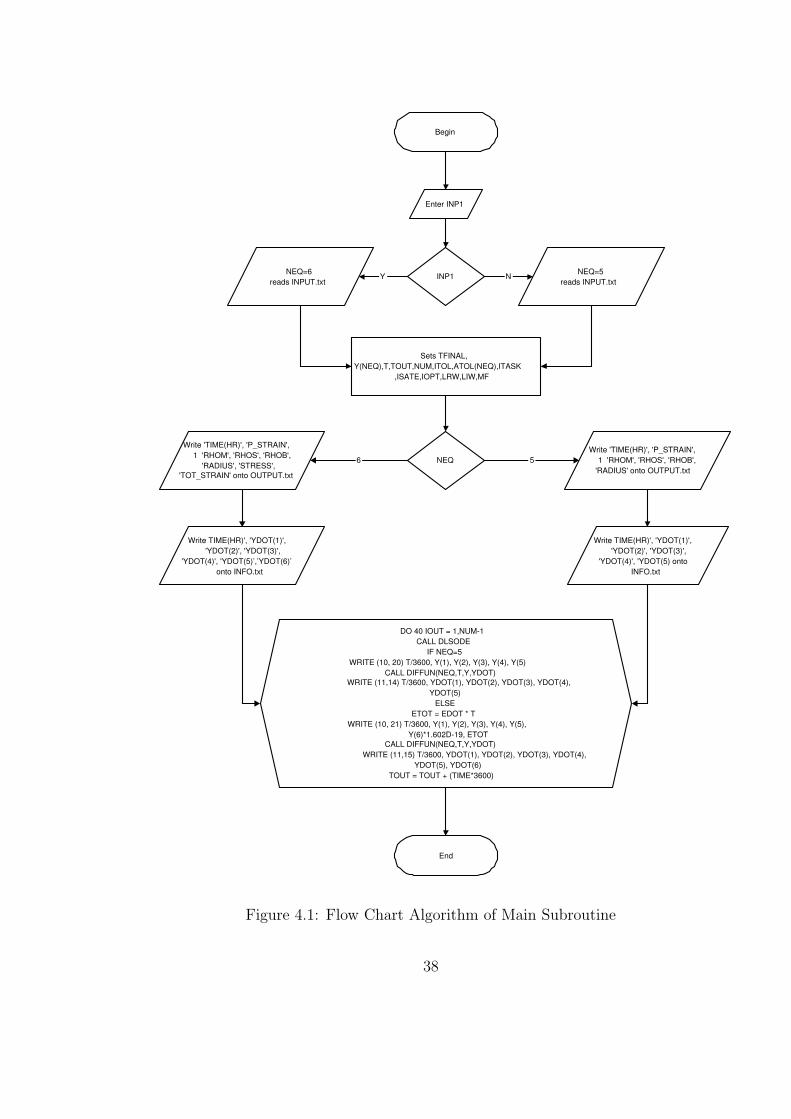
4.1.1 The Main Subroutine

The functions of the main subroutine are to:

• provide an User Interface

• house initial conditions

• call DLSODE subroutine to calculate the values of each dependent variables(ρm,

ρs, etc.,)

• write the output to a text file

The algorithm for the main subroutine are shown on figure 4.1. Note that the

user is allowed to choose to study either creep or constant strain rate test, and

the choice dictates the value of the parameter ”NEQ”, number of equations to

solve. If one chooses to study creep, then NEQ is set to five. If one chooses to

study constant strain rate, then NEQ is set to six. The outputs are then adjusted

accordingly.

37

Begin

Enter INP1

NEQ=6 reads INPUT.txt

INP1 Y NEQ=5

reads INPUT.txt N

Sets TFINAL, Y(NEQ),T,TOUT,NUM,ITOL,ATOL(NEQ),ITASK

,ISATE,IOPT,LRW,LIW,MF

Write TIME(HR)', 'YDOT(1)', 'YDOT(2)', 'YDOT(3)',

'YDOT(4)', 'YDOT(5)’,’YDOT(6)’ onto INFO.txt

NEQ

Write TIME(HR)', 'YDOT(1)', 'YDOT(2)', 'YDOT(3)', 'YDOT(4)', 'YDOT(5) onto

INFO.txt

6 5

Write 'TIME(HR)', 'P_STRAIN', 1 'RHOM', 'RHOS', 'RHOB',

'RADIUS', 'STRESS', 'TOT_STRAIN' onto OUTPUT.txt

Write 'TIME(HR)', 'P_STRAIN', 1 'RHOM', 'RHOS', 'RHOB',

'RADIUS' onto OUTPUT.txt

DO 40 IOUT = 1,NUM-1 CALL DLSODE

IF NEQ=5 WRITE (10, 20) T/3600, Y(1), Y(2), Y(3), Y(4), Y(5)

CALL DIFFUN(NEQ,T,Y,YDOT) WRITE (11,14) T/3600, YDOT(1), YDOT(2), YDOT(3), YDOT(4),

YDOT(5) ELSE

ETOT = EDOT * T WRITE (10, 21) T/3600, Y(1), Y(2), Y(3), Y(4), Y(5),

Y(6)*1.602D-19, ETOT CALL DIFFUN(NEQ,T,Y,YDOT)

WRITE (11,15) T/3600, YDOT(1), YDOT(2), YDOT(3), YDOT(4), YDOT(5), YDOT(6)

TOUT = TOUT + (TIME*3600)

End

Figure 4.1: Flow Chart Algorithm of Main Subroutine

38

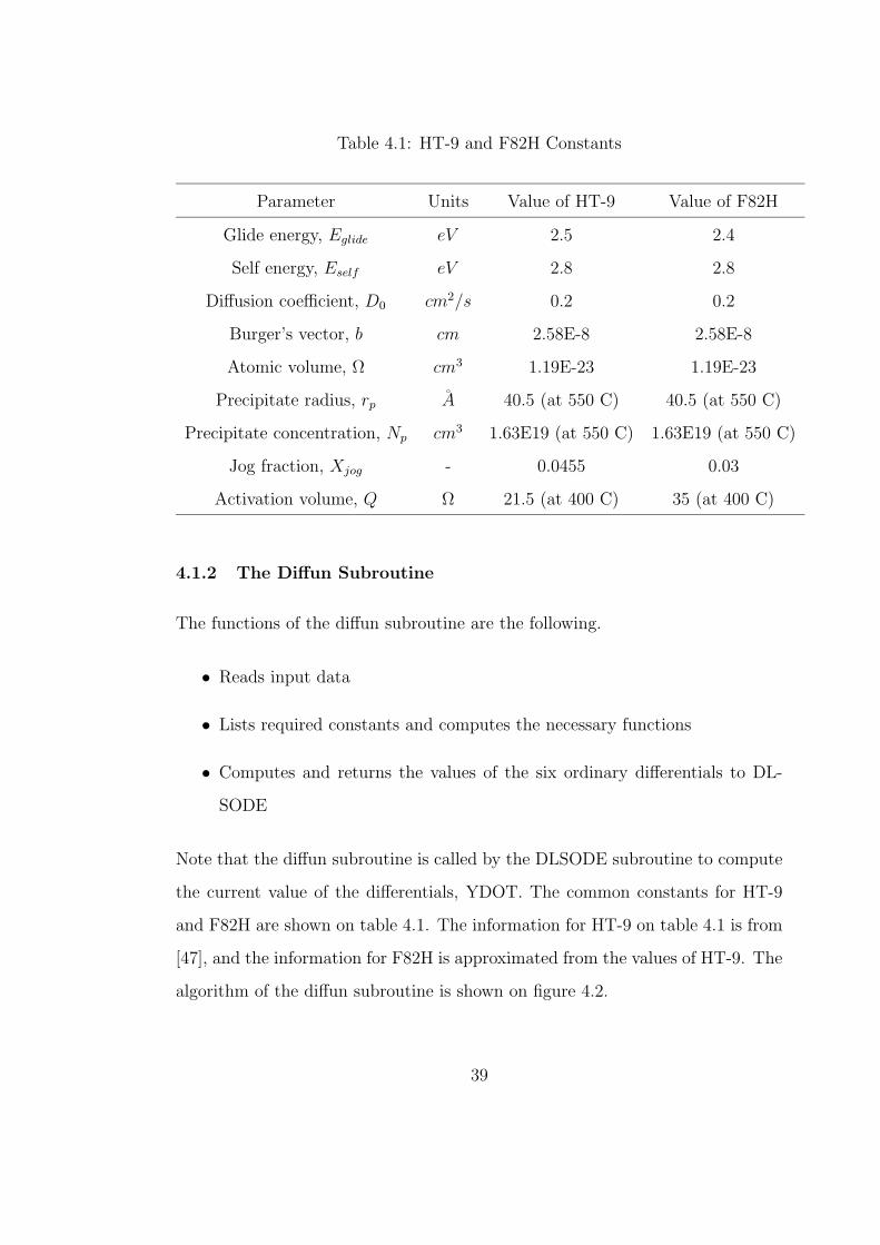
Table 4.1: HT-9 and F82H Constants

Parameter Units Value of HT-9 Value of F82H

Glide energy, Eglide eV 2.5 2.4

Self energy, Eself eV 2.8 2.8

Diffusion coefficient, D0 cm2/s 0.2 0.2

Burger’s vector, b cm 2.58E-8 2.58E-8

Atomic volume, Ω cm3 1.19E-23 1.19E-23

Precipitate radius, rp A 40.5 (at 550 C) 40.5 (at 550 C)

Precipitate concentration, Np cm3 1.63E19 (at 550 C) 1.63E19 (at 550 C)

Jog fraction, Xjog - 0.0455 0.03

Activation volume, Q Ω 21.5 (at 400 C) 35 (at 400 C)

4.1.2 The Diffun Subroutine

The functions of the diffun subroutine are the following.

• Reads input data

• Lists required constants and computes the necessary functions

• Computes and returns the values of the six ordinary differentials to DL-

SODE

Note that the diffun subroutine is called by the DLSODE subroutine to compute

the current value of the differentials, YDOT. The common constants for HT-9

and F82H are shown on table 4.1. The information for HT-9 on table 4.1 is from

[47], and the information for F82H is approximated from the values of HT-9. The

algorithm of the diffun subroutine is shown on figure 4.2.

39

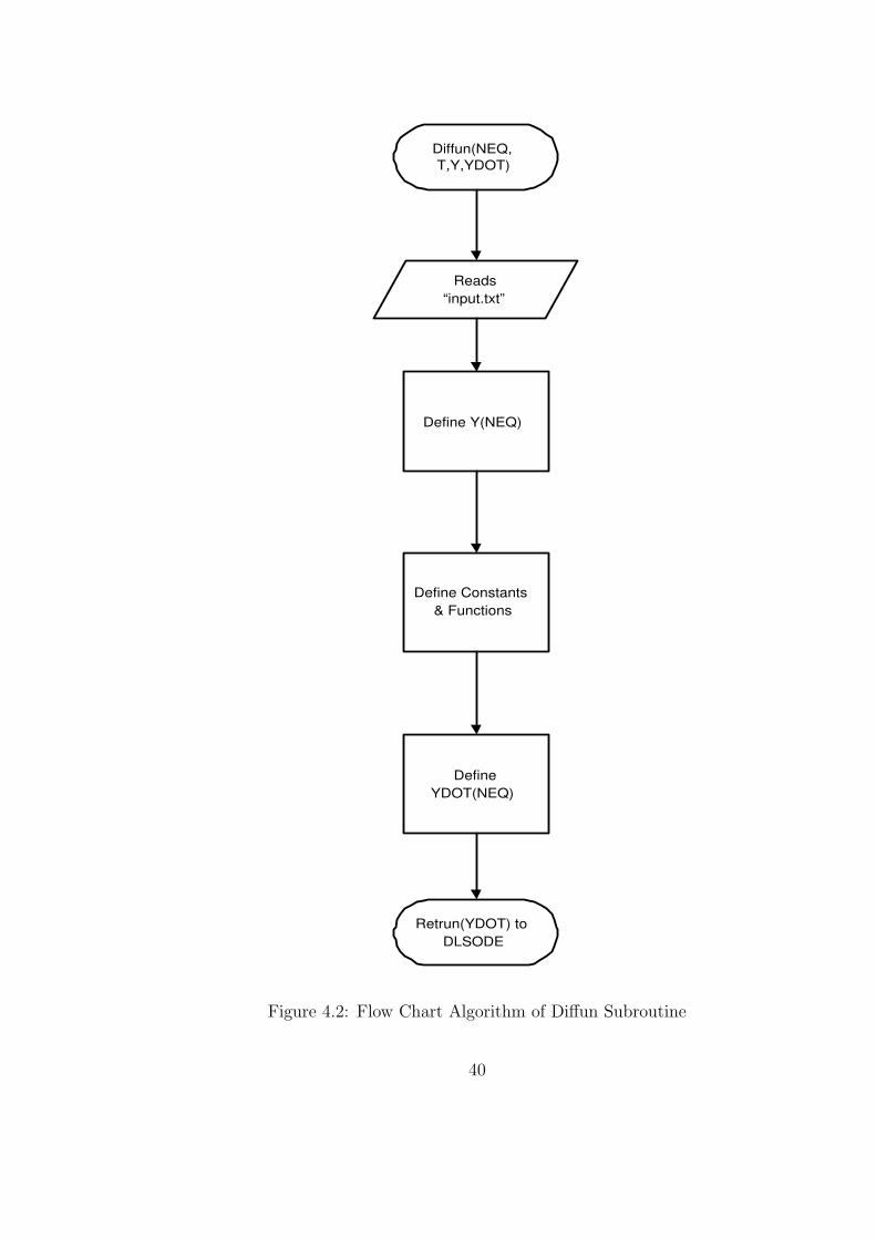
Diffun(NEQ, T,Y,YDOT)

Reads “input.txt”

Define Y(NEQ)

Define Constants & Functions

Define YDOT(NEQ)

Retrun(YDOT) to DLSODE

Figure 4.2: Flow Chart Algorithm of Diffun Subroutine

40

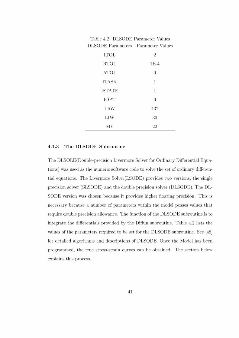
Table 4.2: DLSODE Parameter Values

DLSODE Parameters Parameter Values

ITOL 2

RTOL 1E-4

ATOL 0

ITASK 1

ISTATE 1

IOPT 0

LRW 437

LIW 30

MF 22

4.1.3 The DLSODE Subroutine

The DLSOLE(Double-precision Livermore Solver for Ordinary Differential Equa-

tions) was used as the numeric software code to solve the set of ordinary differen-

tial equations. The Livermore Solver(LSODE) provides two versions, the single

precision solver (SLSODE) and the double precision solver (DLSODE). The DL-

SODE version was chosen because it provides higher floating precision. This is

necessary because a number of parameters within the model posses values that

require double precision allowance. The function of the DLSODE subroutine is to

integrate the differentials provided by the Diffun subroutine. Table 4.2 lists the

values of the parameters required to be set for the DLSODE subroutine. See [48]

for detailed algorithms and descriptions of DLSODE. Once the Model has been

programmed, the true stress-strain curves can be obtained. The section below

explains this process.

41

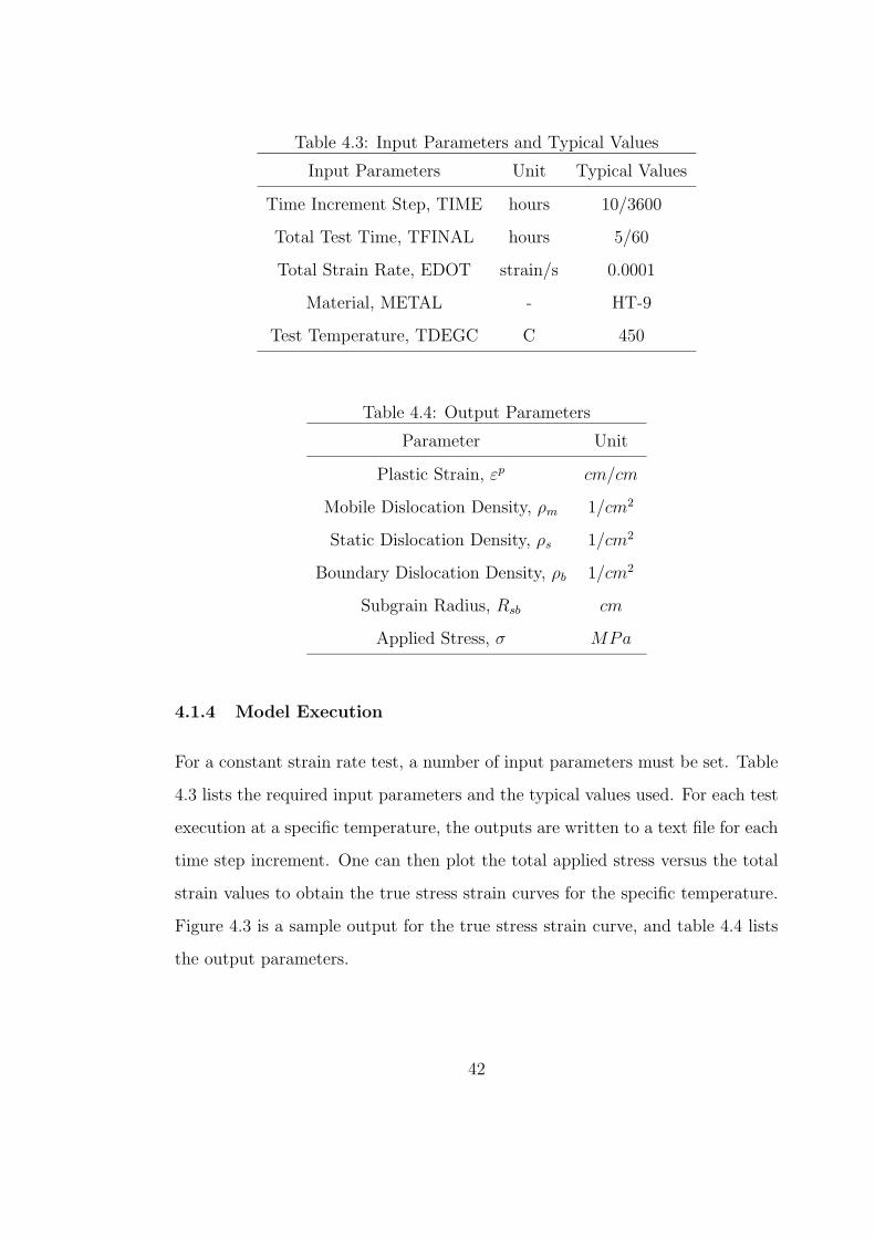
Table 4.3: Input Parameters and Typical Values

Input Parameters Unit Typical Values

Time Increment Step, TIME hours 10/3600

Total Test Time, TFINAL hours 5/60

Total Strain Rate, EDOT strain/s 0.0001

Material, METAL - HT-9

Test Temperature, TDEGC C 450

Table 4.4: Output Parameters

Parameter Unit

Plastic Strain, εp cm/cm

Mobile Dislocation Density, ρm 1/cm2

Static Dislocation Density, ρs 1/cm2

Boundary Dislocation Density, ρb 1/cm2

Subgrain Radius, Rsb cm

Applied Stress, σ MPa

4.1.4 Model Execution

For a constant strain rate test, a number of input parameters must be set. Table

4.3 lists the required input parameters and the typical values used. For each test

execution at a specific temperature, the outputs are written to a text file for each

time step increment. One can then plot the total applied stress versus the total

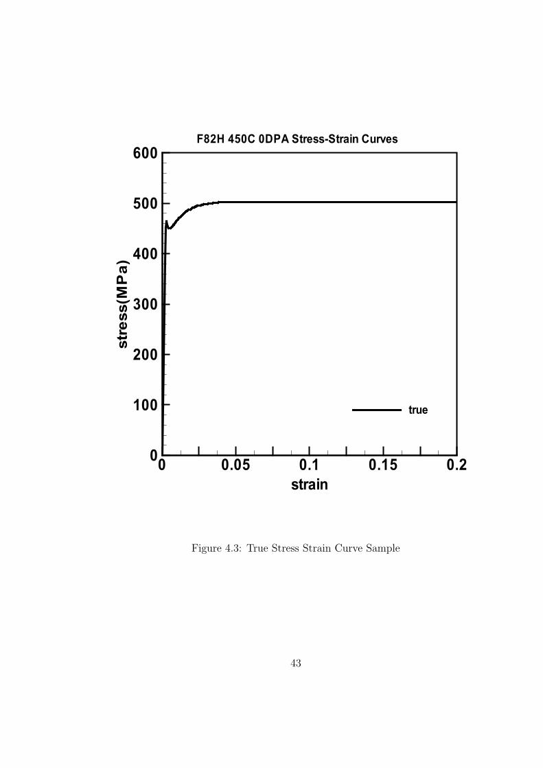
strain values to obtain the true stress strain curves for the specific temperature.

Figure 4.3 is a sample output for the true stress strain curve, and table 4.4 lists

the output parameters.

42

strain

stress(MPa)

0 0.05 0.1 0.15 0.20

100

200

300

400

500

600

true

F82H 450C 0DPA Stress-Strain Curves

Figure 4.3: True Stress Strain Curve Sample

43

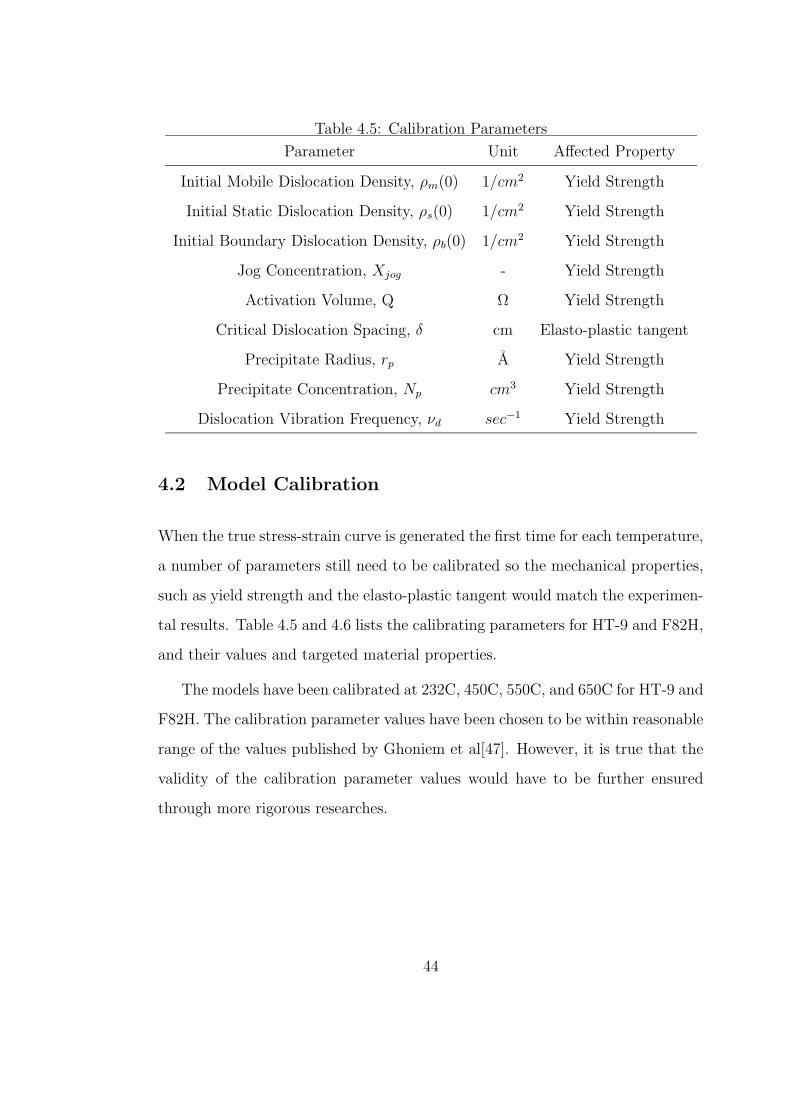
Table 4.5: Calibration Parameters

Parameter Unit Affected Property

Initial Mobile Dislocation Density, ρm(0) 1/cm2 Yield Strength

Initial Static Dislocation Density, ρs(0) 1/cm2 Yield Strength

Initial Boundary Dislocation Density, ρb(0) 1/cm2 Yield Strength

Jog Concentration, Xjog - Yield Strength

Activation Volume, Q Ω Yield Strength

Critical Dislocation Spacing, δ cm Elasto-plastic tangent

Precipitate Radius, rp A Yield Strength

Precipitate Concentration, Np cm3 Yield Strength

Dislocation Vibration Frequency, νd sec−1 Yield Strength

4.2 Model Calibration

When the true stress-strain curve is generated the first time for each temperature,

a number of parameters still need to be calibrated so the mechanical properties,

such as yield strength and the elasto-plastic tangent would match the experimen-

tal results. Table 4.5 and 4.6 lists the calibrating parameters for HT-9 and F82H,

and their values and targeted material properties.

The models have been calibrated at 232C, 450C, 550C, and 650C for HT-9 and

F82H. The calibration parameter values have been chosen to be within reasonable

range of the values published by Ghoniem et al[47]. However, it is true that the

validity of the calibration parameter values would have to be further ensured

through more rigorous researches.

44

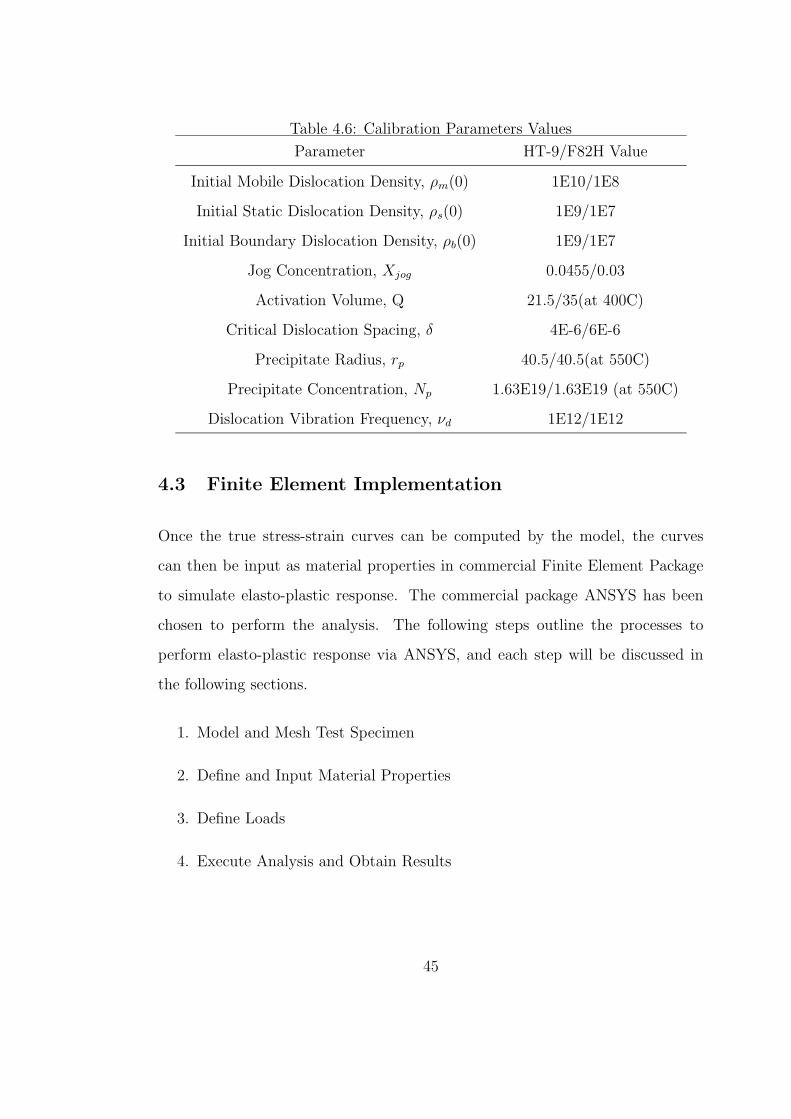
Table 4.6: Calibration Parameters Values

Parameter HT-9/F82H Value

Initial Mobile Dislocation Density, ρm(0) 1E10/1E8

Initial Static Dislocation Density, ρs(0) 1E9/1E7

Initial Boundary Dislocation Density, ρb(0) 1E9/1E7

Jog Concentration, Xjog 0.0455/0.03

Activation Volume, Q 21.5/35(at 400C)

Critical Dislocation Spacing, δ 4E-6/6E-6

Precipitate Radius, rp 40.5/40.5(at 550C)

Precipitate Concentration, Np 1.63E19/1.63E19 (at 550C)

Dislocation Vibration Frequency, νd 1E12/1E12

4.3 Finite Element Implementation

Once the true stress-strain curves can be computed by the model, the curves

can then be input as material properties in commercial Finite Element Package

to simulate elasto-plastic response. The commercial package ANSYS has been

chosen to perform the analysis. The following steps outline the processes to

perform elasto-plastic response via ANSYS, and each step will be discussed in

the following sections.

1. Model and Mesh Test Specimen

2. Define and Input Material Properties

3. Define Loads

4. Execute Analysis and Obtain Results

45

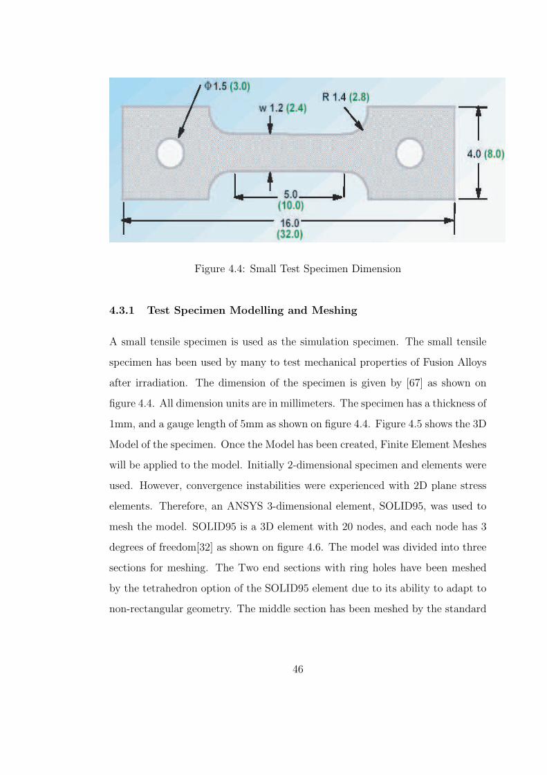
Figure 4.4: Small Test Specimen Dimension

4.3.1 Test Specimen Modelling and Meshing

A small tensile specimen is used as the simulation specimen. The small tensile

specimen has been used by many to test mechanical properties of Fusion Alloys

after irradiation. The dimension of the specimen is given by [67] as shown on

figure 4.4. All dimension units are in millimeters. The specimen has a thickness of

1mm, and a gauge length of 5mm as shown on figure 4.4. Figure 4.5 shows the 3D

Model of the specimen. Once the Model has been created, Finite Element Meshes

will be applied to the model. Initially 2-dimensional specimen and elements were

used. However, convergence instabilities were experienced with 2D plane stress

elements. Therefore, an ANSYS 3-dimensional element, SOLID95, was used to

mesh the model. SOLID95 is a 3D element with 20 nodes, and each node has 3

degrees of freedom[32] as shown on figure 4.6. The model was divided into three

sections for meshing. The Two end sections with ring holes have been meshed

by the tetrahedron option of the SOLID95 element due to its ability to adapt to

non-rectangular geometry. The middle section has been meshed by the standard

46

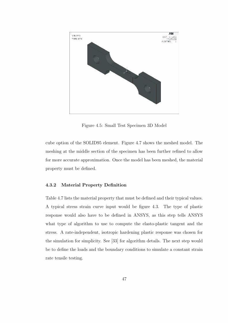
Figure 4.5: Small Test Specimen 3D Model

cube option of the SOLID95 element. Figure 4.7 shows the meshed model. The

meshing at the middle section of the specimen has been further refined to allow

for more accurate approximation. Once the model has been meshed, the material

property must be defined.

4.3.2 Material Property Definition

Table 4.7 lists the material property that must be defined and their typical values.

A typical stress strain curve input would be figure 4.3. The type of plastic

response would also have to be defined in ANSYS, as this step tells ANSYS

what type of algorithm to use to compute the elasto-plastic tangent and the

stress. A rate-independent, isotropic hardening plastic response was chosen for

the simulation for simplicity. See [33] for algorithm details. The next step would

be to define the loads and the boundary conditions to simulate a constant strain

rate tensile testing.

47

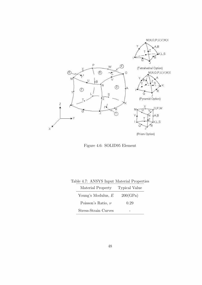
Figure 4.6: SOLID95 Element

Table 4.7: ANSYS Input Material Properties

Material Property Typical Value

Young’s Modulus, E 200(GPa)

Poisson’s Ratio, ν 0.29

Stress-Strain Curves -

48

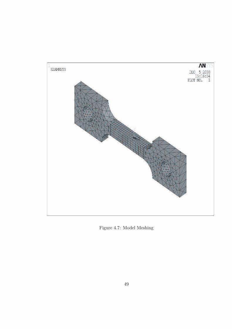
Figure 4.7: Model Meshing

49

4.3.3 Load Definition

The controlling parameter of the simulation is the displacement, and the nodal

forces were extracted from the simulation. The gauge length of the specimen is

taken to be 5 mm as shown on figure 4.4. The Model is prescribed to be fixed

at the left edge of the left pin hole. The displacement boundary condition is

prescribed at the right edge of the right pin hole as shown on figure 4.8. The

displacement must be divided into small ”load steps” in order for the algorithm

to converge successfully. Figure 4.9 shows typical displacement load points on

the engineering stress-strain curve. Each point on curve is a load point. Once the

loads have been defined, the analysis can then be executed, and the engineering

curve can then be extrapolated. To avoid local plastic deformation around the

pin holes, the modulus of the two end sections with the pin holes have been

raised to 2E20 so all displacement loads can be directly transferred to the middle

section.

4.3.4 Analysis Execution and Results

It normally takes thirty to forty minutes to complete ten to fifteen load steps of

calculation. The results are then post-processed and analyzed. The nodal forces

on the left of the pin holes are summed to obtained the engineering stress. The

following chapter provides and discusses the results.

50

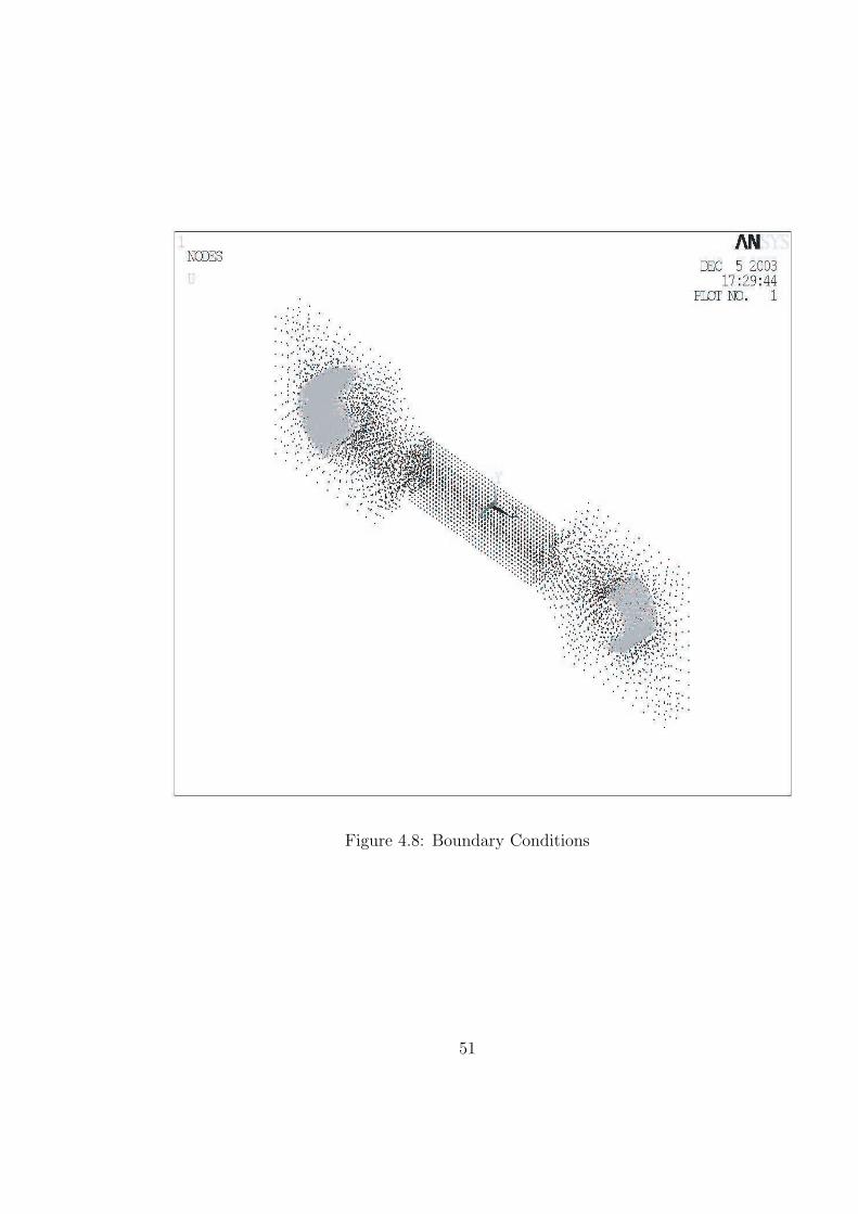
Figure 4.8: Boundary Conditions

51

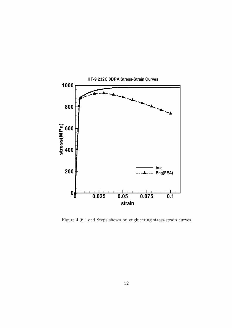
strain

stress(MPa)

0 0.025 0.05 0.075 0.10

200

400

600

800

1000

true

Eng(FEA)

HT-9 232C 0DPA Stress-Strain Curves

Figure 4.9: Load Steps shown on engineering stress-strain curves

52

CHAPTER 5

Results and Experimental Model Validation

The objective of this chapter is to show and discuss the results from implement-

ing the Dislocation-based Constitutive Model, and from performing elasto-plastic

Finite Element Analysis with the predicted true stress-strain curves. The results

from the FORTRAN90 implementation will be shown and discussed first, fol-

lowed by the Finite Element Analysis results, and a brief analysis of the plastic

instability phenomenon.

5.1 FORTRAN90 Implementation Results

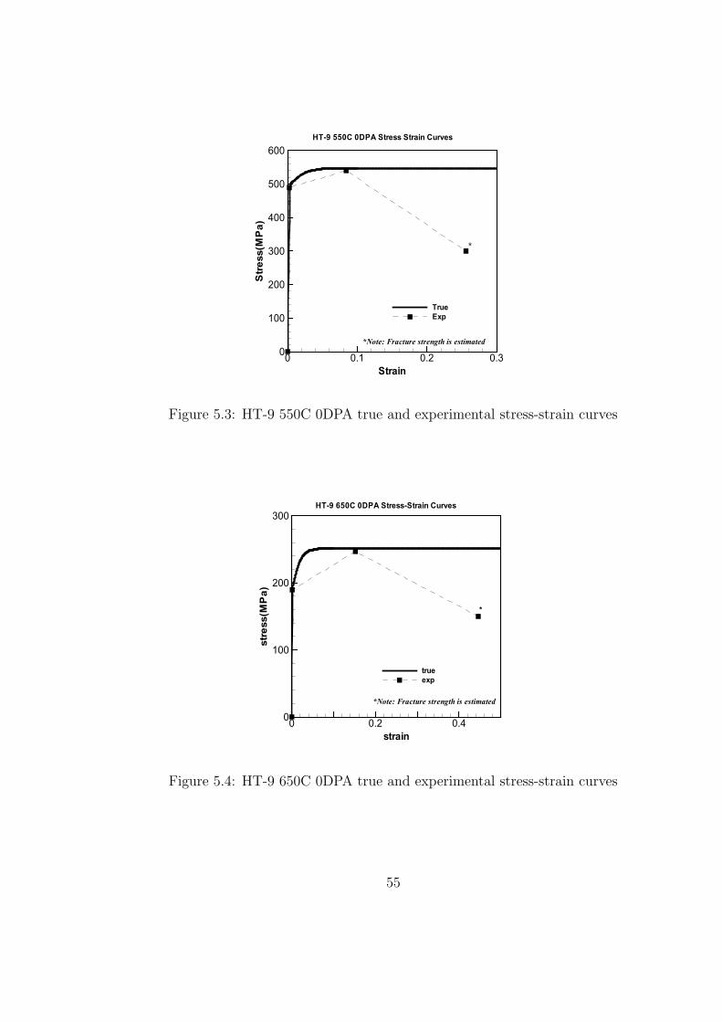
The model was executed for HT-9 and F82H at 232C, 450C, 550C, and 650C.

There were total of eight input files created, and eight output files generated for

each scenario. The sample input and output files are shown on appendix B and

C. The total strain and stress are then plotted to obtain the true stress-strain

curves for each scenario as shown on figure 5.1 to 5.8. The experimental results

were obtained from [58] and [55], and have been plotted on figure 5.1 to 5.8 as

well. However, only the yield strength, ultimate strength, uniform strain, and

total strains were published on [58] and [55]. Therefore, the experimental fracture

strength has been estimated.

It can be observed that the yield strength, Young’s Modulus, the ultimate

strength, and the elasto-plastic tangent from the FORTRAN implementation

53

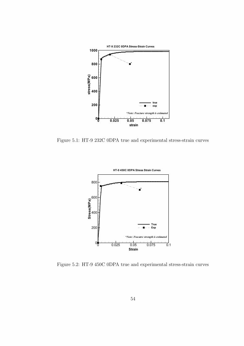
strain

stress(MPa)

0 0.025 0.05 0.075 0.10

200

400

600

800

1000

true

exp


*

*Note: Fracture strength is estimated

Figure 5.1: HT-9 232C 0DPA true and experimental stress-strain curves

Strain

Stress(MPa)

0 0.025 0.05 0.075 0.10

200

400

600

800

True

Exp

HT-9 450C 0DPA Stress Strain Curves

*

*Note: Fracutre strength is estimated


54

Strain

Stress(MPa)

0 0.1 0.2 0.30

100

200

300

400

500

600

True

Exp


*



strain

stress(MPa)

0 0.2 0.40

100

200

300

true

exp


*



55

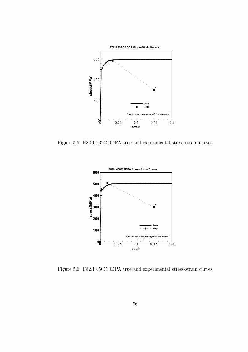
strain

stress(MPa)

0 0.05 0.1 0.15 0.20

200

400

600

true

exp



*

Figure 5.5: F82H 232C 0DPA true and experimental stress-strain curves

strain

stress(MPa)

0 0.05 0.1 0.15 0.20

100

200

300

400

500

600

true

exp


*

*Note: Fracture Strength is estimated


56

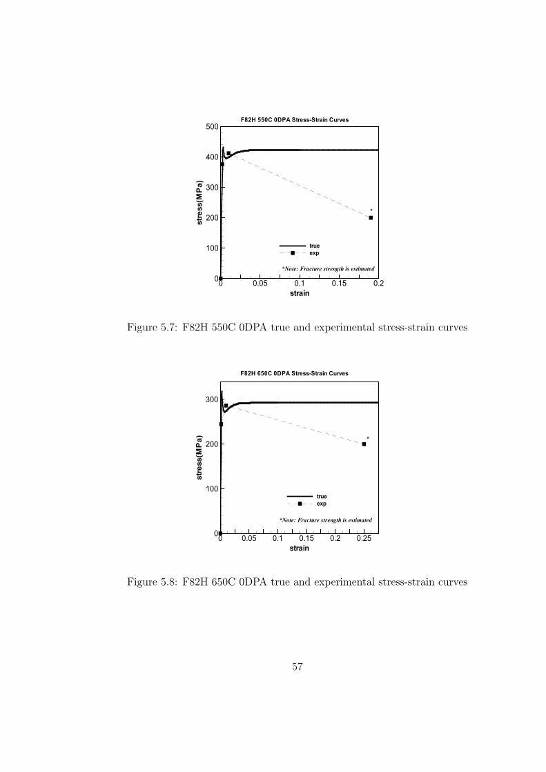
strain

stress(MPa)

0 0.05 0.1 0.15 0.20

100

200

300

400

500

true

exp


*



strain

stress(MPa)

0 0.05 0.1 0.15 0.2 0.250

100

200

300

true

exp


*



57

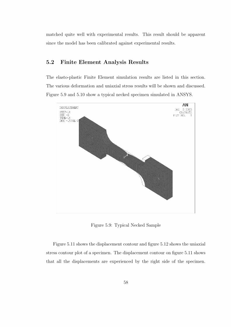
matched quite well with experimental results. This result should be apparent

since the model has been calibrated against experimental results.

5.2 Finite Element Analysis Results

The elasto-plastic Finite Element simulation results are listed in this section.

The various deformation and uniaxial stress results will be shown and discussed.

Figure 5.9 and 5.10 show a typical necked specimen simulated in ANSYS.

Figure 5.9: Typical Necked Sample

Figure 5.11 shows the displacement contour and figure 5.12 shows the uniaxial

stress contour plot of a specimen. The displacement contour on figure 5.11 shows

that all the displacements are experienced by the right side of the specimen.

58

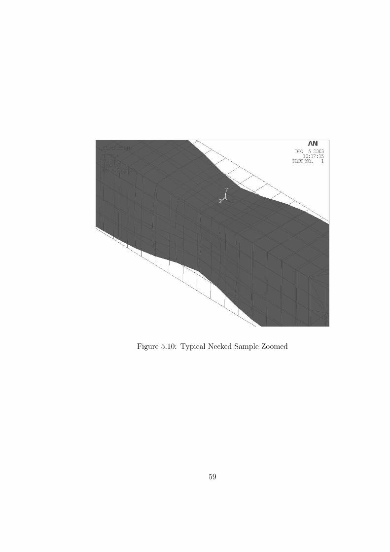
Figure 5.10: Typical Necked Sample Zoomed

59

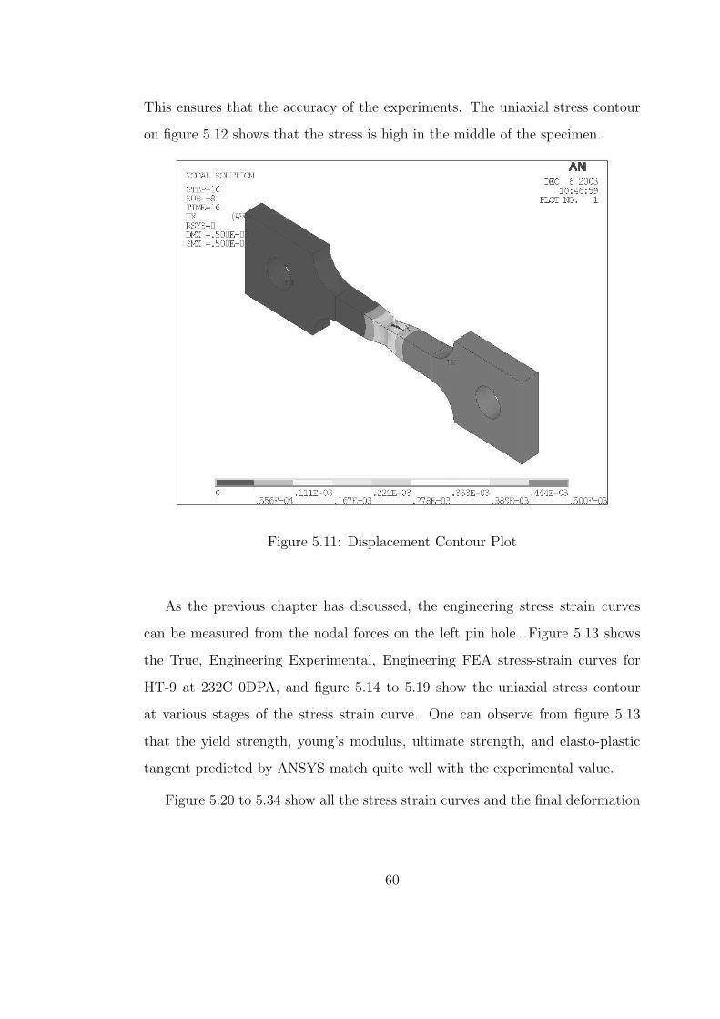
This ensures that the accuracy of the experiments. The uniaxial stress contour

on figure 5.12 shows that the stress is high in the middle of the specimen.

Figure 5.11: Displacement Contour Plot

As the previous chapter has discussed, the engineering stress strain curves

can be measured from the nodal forces on the left pin hole. Figure 5.13 shows

the True, Engineering Experimental, Engineering FEA stress-strain curves for

HT-9 at 232C 0DPA, and figure 5.14 to 5.19 show the uniaxial stress contour

at various stages of the stress strain curve. One can observe from figure 5.13

that the yield strength, young’s modulus, ultimate strength, and elasto-plastic

tangent predicted by ANSYS match quite well with the experimental value.

Figure 5.20 to 5.34 show all the stress strain curves and the final deformation

60

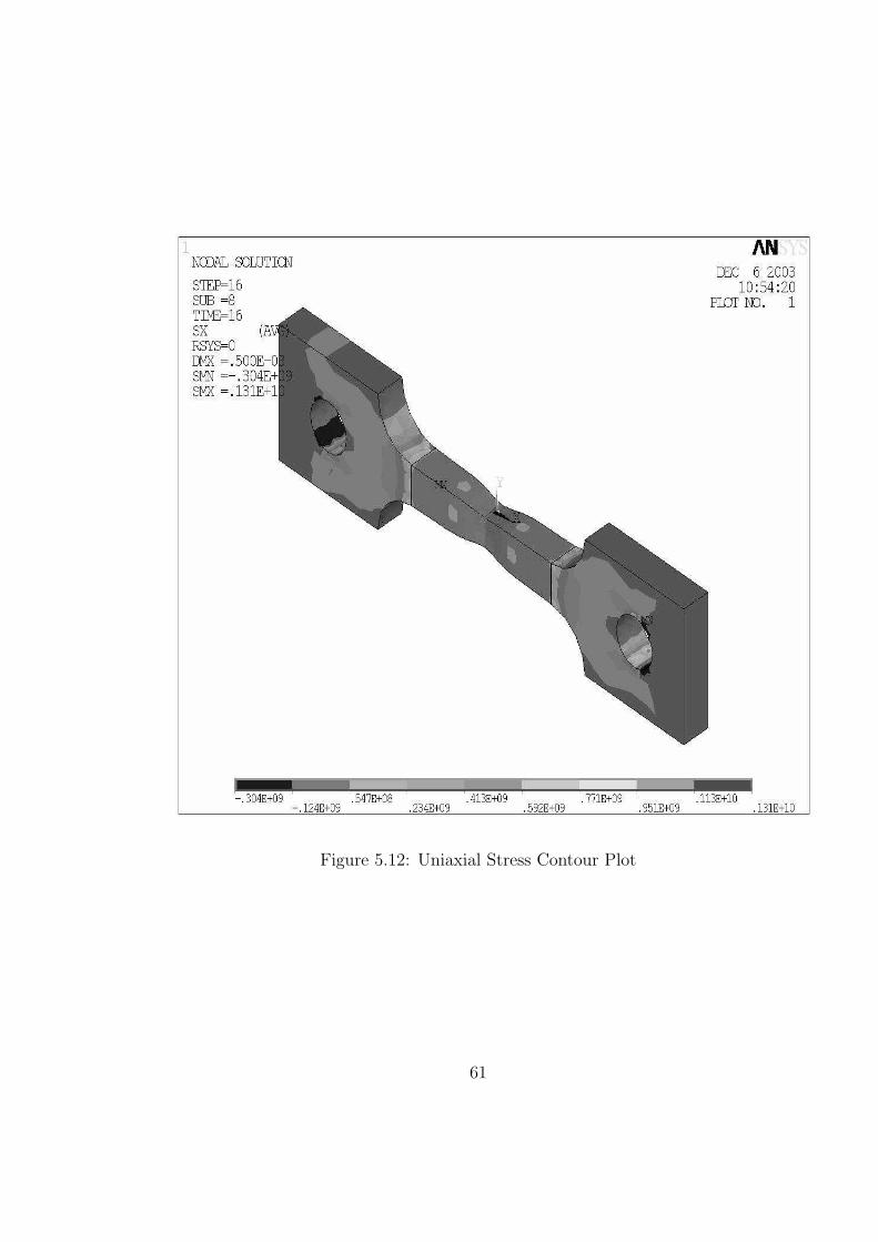
Figure 5.12: Uniaxial Stress Contour Plot

61

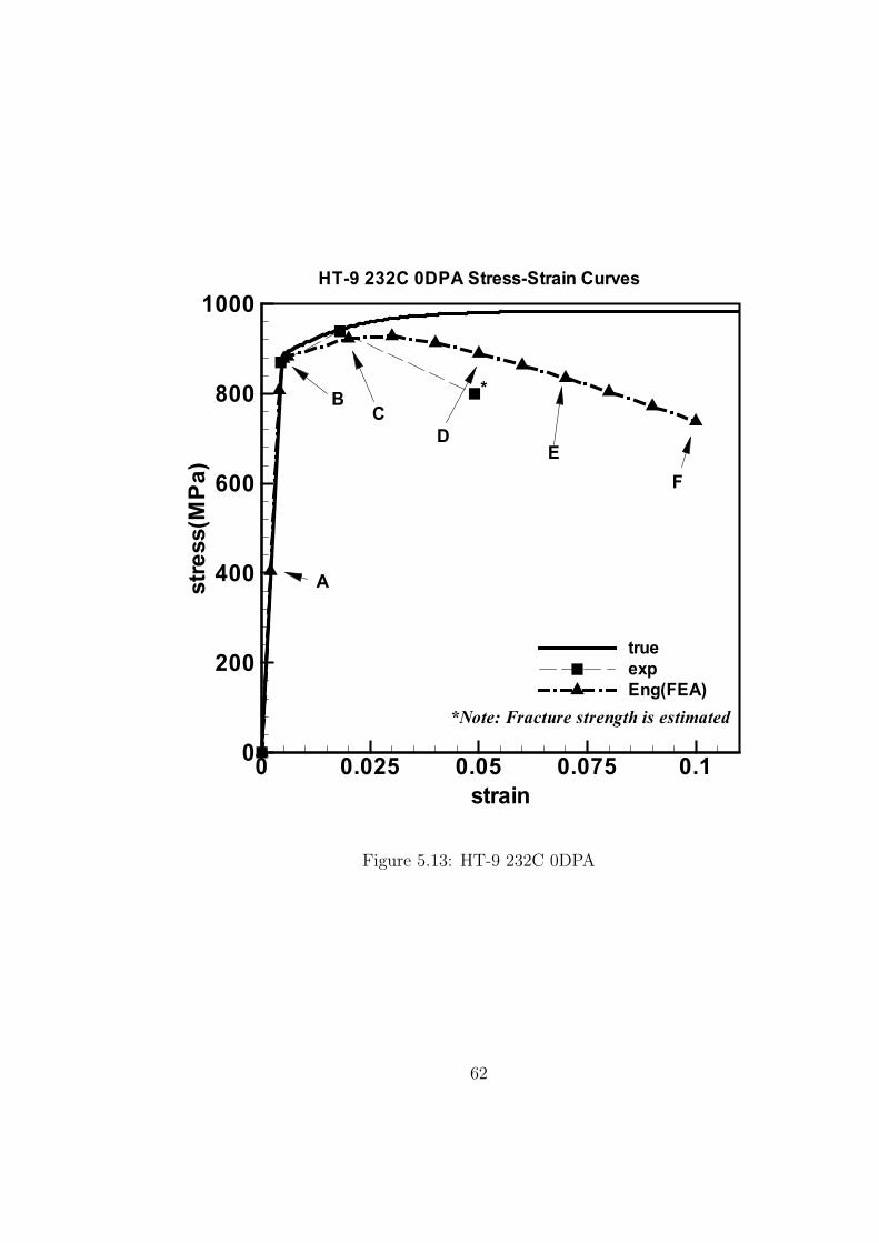
strain

stress(MPa)

0 0.025 0.05 0.075 0.10

200

400

600

800

1000

true

exp

Eng(FEA)


A

BC

DE

F

*


Figure 5.13: HT-9 232C 0DPA

62

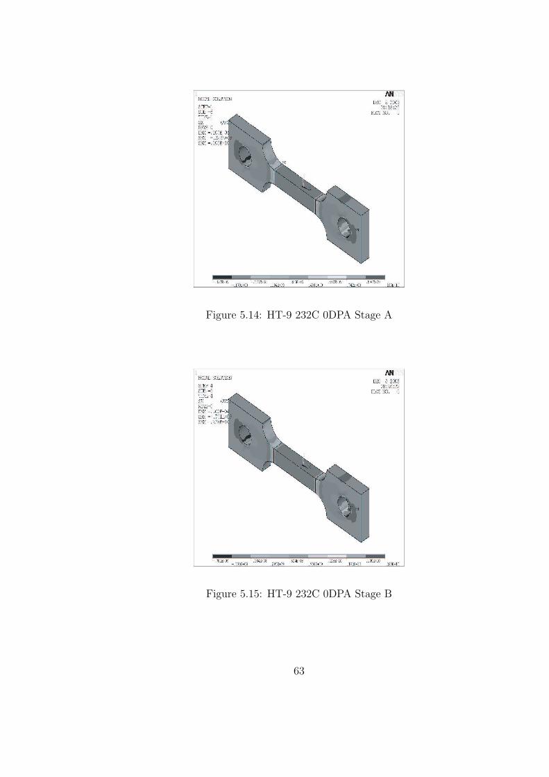
Figure 5.14: HT-9 232C 0DPA Stage A

Figure 5.15: HT-9 232C 0DPA Stage B

63

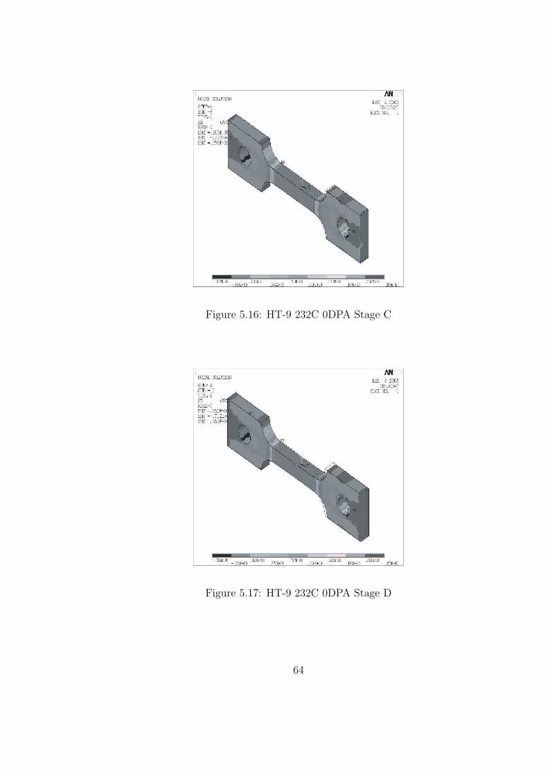
Figure 5.16: HT-9 232C 0DPA Stage C

Figure 5.17: HT-9 232C 0DPA Stage D

64

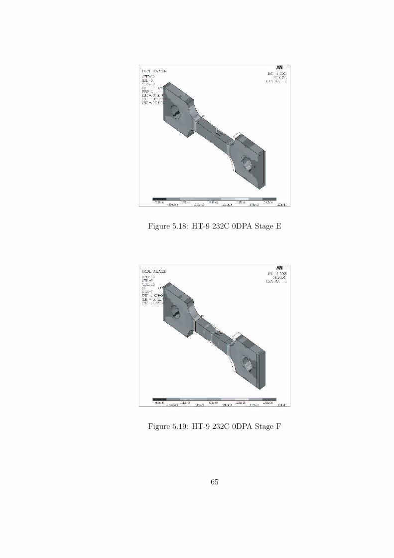
Figure 5.18: HT-9 232C 0DPA Stage E

Figure 5.19: HT-9 232C 0DPA Stage F

65

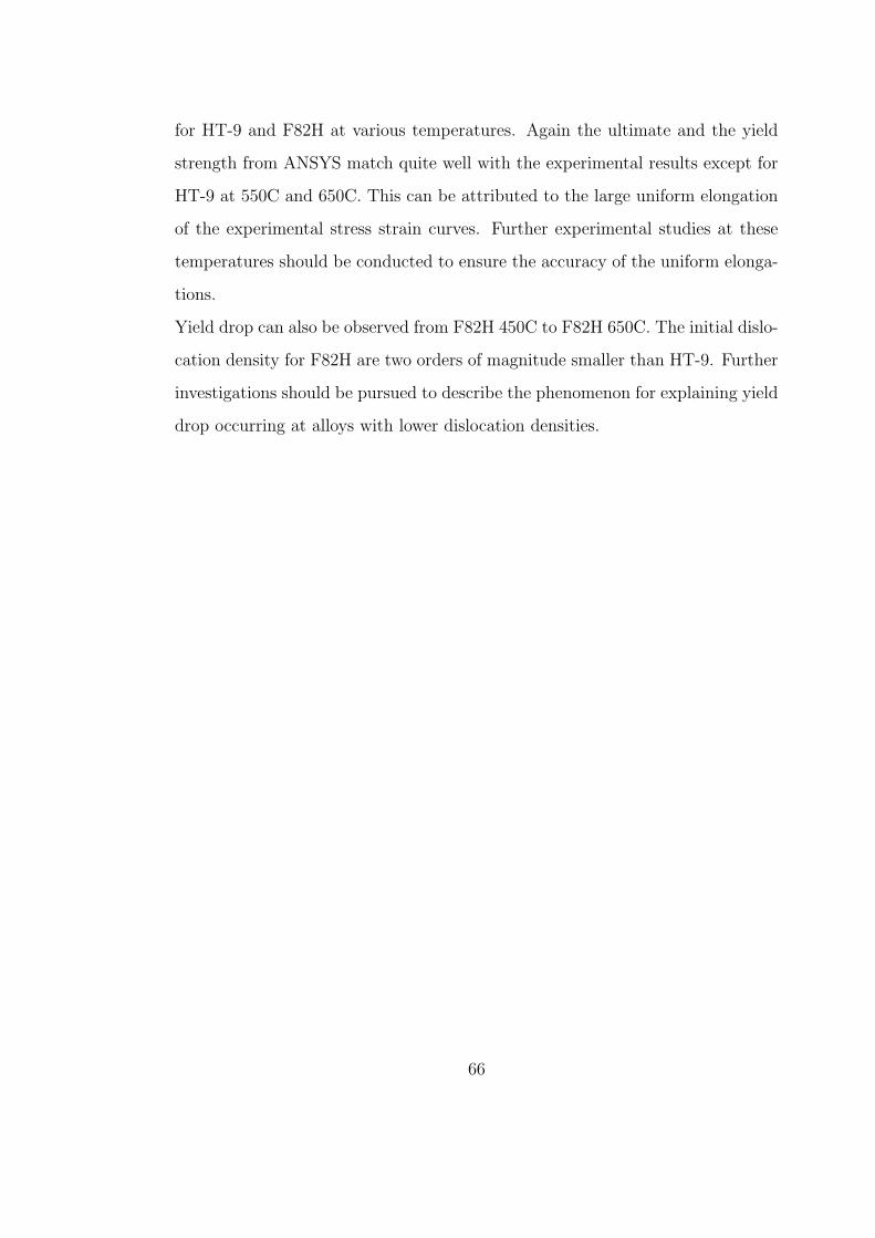
for HT-9 and F82H at various temperatures. Again the ultimate and the yield

strength from ANSYS match quite well with the experimental results except for

HT-9 at 550C and 650C. This can be attributed to the large uniform elongation

of the experimental stress strain curves. Further experimental studies at these

temperatures should be conducted to ensure the accuracy of the uniform elonga-

tions.

Yield drop can also be observed from F82H 450C to F82H 650C. The initial dislo-

cation density for F82H are two orders of magnitude smaller than HT-9. Further

investigations should be pursued to describe the phenomenon for explaining yield

drop occurring at alloys with lower dislocation densities.

66

strain

stress(MPa)

0 0.025 0.05 0.075 0.10

200

400

600

800

1000

true

exp

Eng(FEA)


*


Figure 5.20: HT-9 232C 0DPA stress-strain curves

Figure 5.21: HT-9 232C 0DPA Final Displacement

67

Strain

Stress(MPa)

0 0.025 0.05 0.075 0.10

200

400

600

800

True

Exp

Eng(FEA)


*




68

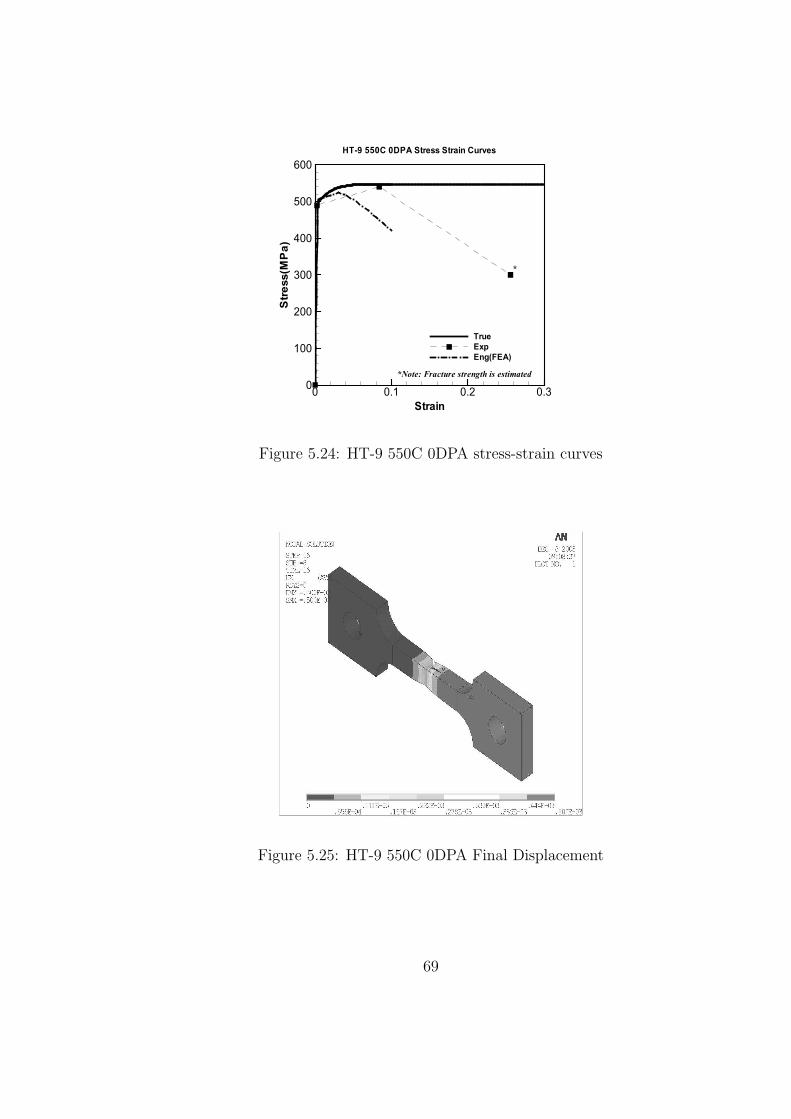
Strain

Stress(MPa)

0 0.1 0.2 0.30

100

200

300

400

500

600

True

Exp

Eng(FEA)


*




69

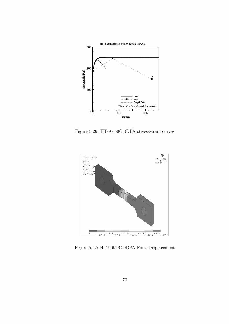
strain

stress(MPa)

0 0.2 0.40

100

200

300

true

exp

Eng(FEA)


*




70

strain

stress(MPa)

0 0.05 0.1 0.15 0.20

200

400

600

true

exp

Eng(FEA)



*

Figure 5.28: F82H 232C 0DPA stress-strain curves

Figure 5.29: F82H 232C 0DPA Final Displacement

71

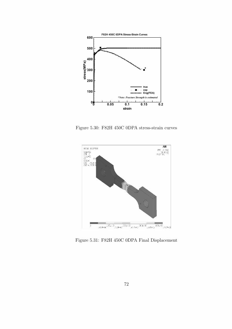
strain

stress(MPa)

0 0.05 0.1 0.15 0.20

100

200

300

400

500

600

true

exp

Eng(FEA)


*

*Note: Fracture Strength is estimated



72

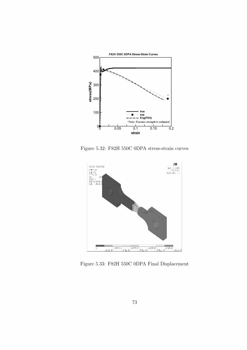
strain

stress(MPa)

0 0.05 0.1 0.15 0.20

100

200

300

400

500

true

exp

Eng(FEA)


*




73

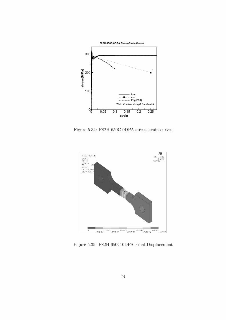
strain

stress(MPa)

0 0.05 0.1 0.15 0.2 0.250

100

200

300

true

exp

Eng(FEA)


*




74

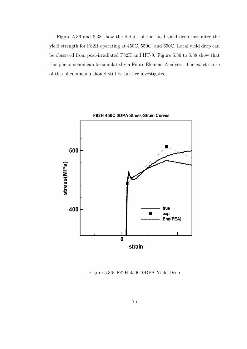
Figure 5.36 and 5.38 show the details of the local yield drop just after the

yield strength for F82H operating at 450C, 550C, and 650C. Local yield drop can

be observed from post-irradiated F82H and HT-9. Figure 5.36 to 5.38 show that

this phenomenon can be simulated via Finite Element Analysis. The exact cause

of this phenomenon should still be further investigated.

strain

stress(MPa)

0

400

500

true

exp

Eng(FEA)


Figure 5.36: F82H 450C 0DPA Yield Drop

75

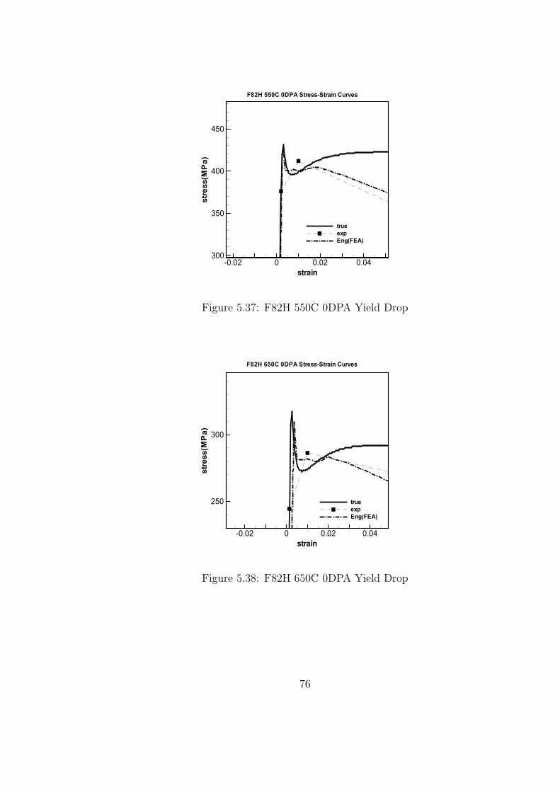
strain

stress(MPa)

-0.02 0 0.02 0.04300

350

400

450

true

exp

Eng(FEA)



strain

stress(MPa)

-0.02 0 0.02 0.04

250

300

true

exp

Eng(FEA)



76

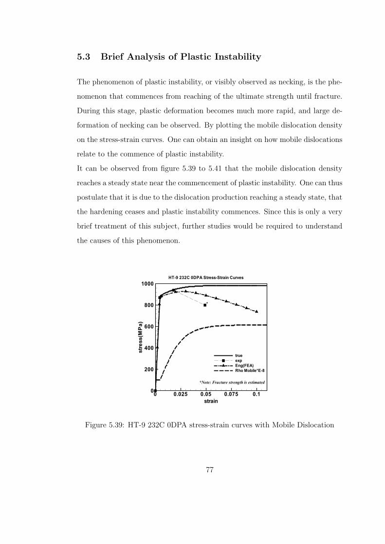
5.3 Brief Analysis of Plastic Instability

The phenomenon of plastic instability, or visibly observed as necking, is the phe-

nomenon that commences from reaching of the ultimate strength until fracture.

During this stage, plastic deformation becomes much more rapid, and large de-

formation of necking can be observed. By plotting the mobile dislocation density

on the stress-strain curves. One can obtain an insight on how mobile dislocations

relate to the commence of plastic instability.

It can be observed from figure 5.39 to 5.41 that the mobile dislocation density

reaches a steady state near the commencement of plastic instability. One can thus

postulate that it is due to the dislocation production reaching a steady state, that

the hardening ceases and plastic instability commences. Since this is only a very

brief treatment of this subject, further studies would be required to understand

the causes of this phenomenon.

strain

stress(MPa)

0 0.025 0.05 0.075 0.10

200

400

600

800

1000

true

exp

Eng(FEA)

Rho Mobile*E-8


*


Figure 5.39: HT-9 232C 0DPA stress-strain curves with Mobile Dislocation

77

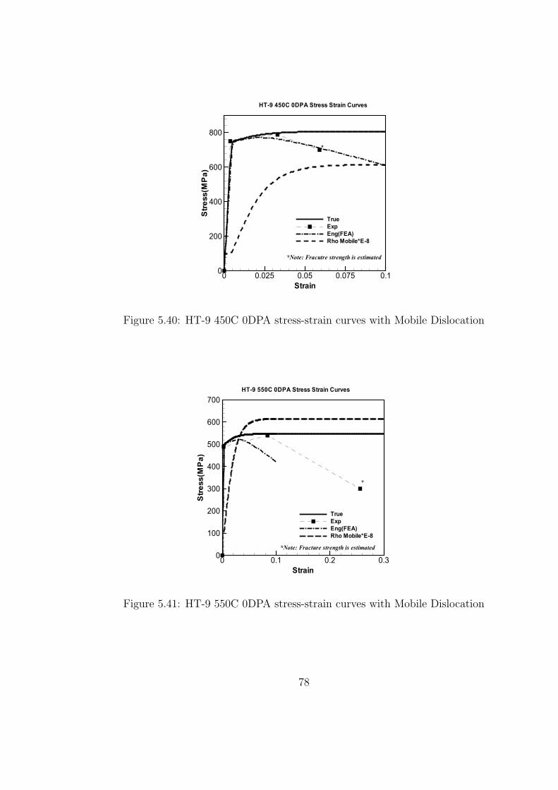
Strain

Stress(MPa)

0 0.025 0.05 0.075 0.10

200

400

600

800

True

Exp

Eng(FEA)

Rho Mobile*E-8


*



Strain

Stress(MPa)

0 0.1 0.2 0.30

100

200

300

400

500

600

700

True

Exp

Eng(FEA)

Rho Mobile*E-8


*



78

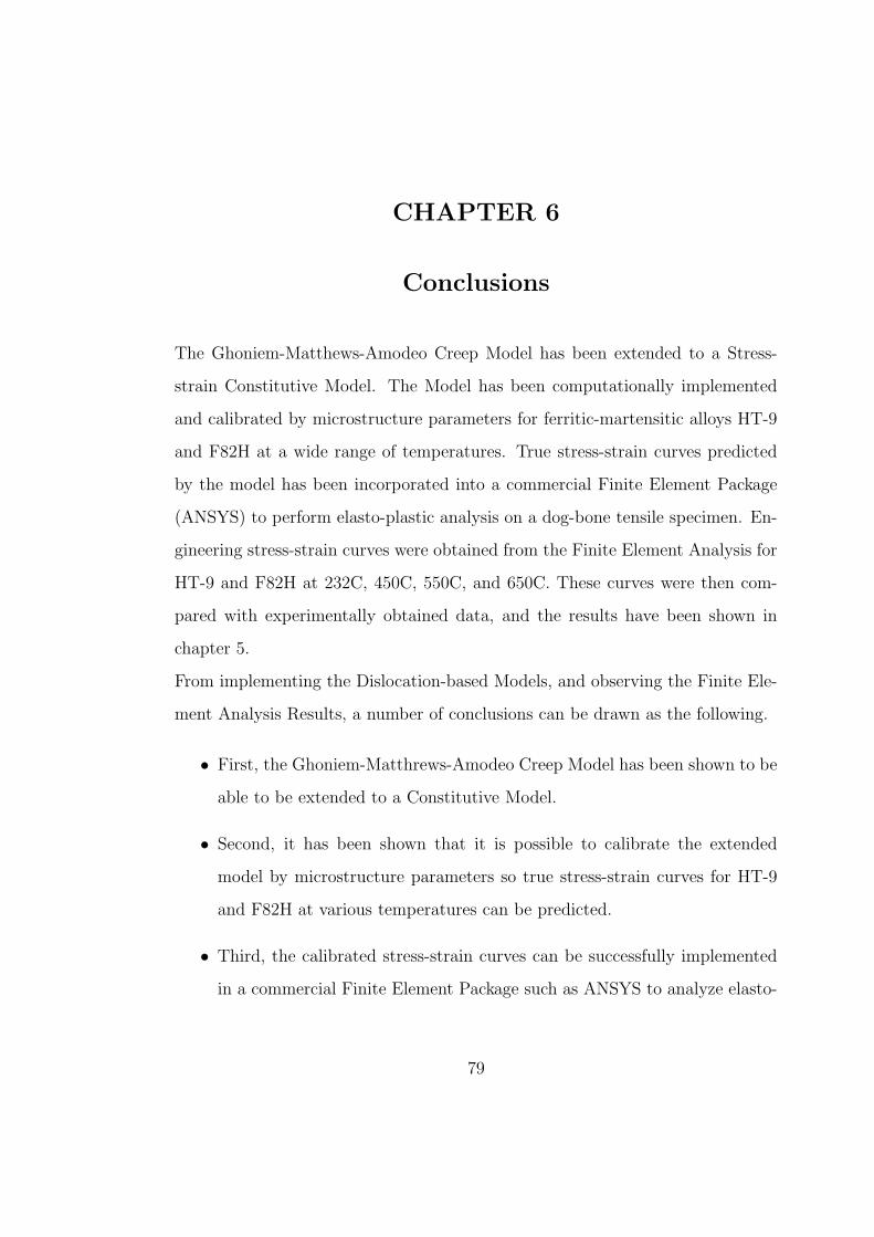
CHAPTER 6

Conclusions

The Ghoniem-Matthews-Amodeo Creep Model has been extended to a Stress-

strain Constitutive Model. The Model has been computationally implemented

and calibrated by microstructure parameters for ferritic-martensitic alloys HT-9

and F82H at a wide range of temperatures. True stress-strain curves predicted

by the model has been incorporated into a commercial Finite Element Package

(ANSYS) to perform elasto-plastic analysis on a dog-bone tensile specimen. En-

gineering stress-strain curves were obtained from the Finite Element Analysis for

HT-9 and F82H at 232C, 450C, 550C, and 650C. These curves were then com-

pared with experimentally obtained data, and the results have been shown in

chapter 5.

From implementing the Dislocation-based Models, and observing the Finite Ele-

ment Analysis Results, a number of conclusions can be drawn as the following.

• First, the Ghoniem-Matthrews-Amodeo Creep Model has been shown to be

able to be extended to a Constitutive Model.

• Second, it has been shown that it is possible to calibrate the extended

model by microstructure parameters so true stress-strain curves for HT-9

and F82H at various temperatures can be predicted.

• Third, the calibrated stress-strain curves can be successfully implemented

in a commercial Finite Element Package such as ANSYS to analyze elasto-

79

plastic material deformations.

• Fourth, the plastic instability and necking effect can potentially be a func-

tion of the rate of production of dislocations

The first conclusion can be drawn because true stress-stress curves can be ob-

tained from the extended model. A true stress-strain curve can be obtained from

solving equations from section 3.9 on page 34. The values of the applied stress,

σ and the input total strain ε are plotted to obtain the true stress-strain curves.

Figure 4.3 on page 43 shows the typical true stress strain curve. This technique

is different from a constitutive model that evolves over strain, such as the KM

Model shown earlier. The results however, showed very close resemblance to the

actual steel alloy stress-strain behaviors as one can see from figure 5.20 to 5.38

from page 67 to page 76.

The second conclusion can be drawn because critical features on the true stress-

strain curve can be calibrated via microstructure parameters. These critical fea-

tures include the yield strength, ultimate strength, Young’s Modulus, and the

elasto-plastic tangent. The calibration parameters have been summarized on fig-

ure 4.5 and 4.6 on page 45. It can be observed that the yield strength is the

most sensitive to initial dislocation density ρ(0), activation volume Ω, precipitate

parameters Np and rp, and dislocation vibrational frequency νd. It is well known

that the yield strength can be calibrated against the square root of the dislocation

density. The effects of precipitates and dislocation vibrational frequency are also

well known. However, the effect of activation volume Ω is less well known. From

[30], the effect of activation volume can be related to the activation energy U as

the following,

U = U0 − v(τ − τG) (6.1)

80

where U0 is the local energy barrier, v is the activation volume, and τ and τG are

the flow stress and the temperature independent component of the flow stress. If

the activation volume is increased, then less activation energy would be require to

initiate the flow stress. This can possibly explain the validity of using activation

volume as a calibrating parameter. However, further study should be pursued

to ensure the validity of this calibrating parameter. The hardening rate can be

calibrated by the critical dislocation spacing parameter δ due to dynamic recovery.

The value used for this parameter is approximately 40-60 nm. This match the

results published by Essmann et al [14] quite well, which is 50-500 nm for screw

and 1.6 nm for edge dislocations(in copper).

The third conclusion can be drawn because the engineering stress-strain curves

obtained from FEA show reasonable match to the experimental values. The

yield and ultimate strength obtained from ANSYS as shown on figure 5.20 to

5.38 from page 67 to 76 correspond quite well with experimental results. The

effect of necking and local strain softening can also be observed as shown on

numerous figures in chapter 5.

The fourth conclusion can be drawn by observing figure 5.39 to 5.41 on chapter 5.

As the previous chapter had discussed, plastic instability can be observed when

mobile dislocation production reaches a steady state. Further studies have to be

done in order to strength this conclusion. However, one should be able to safely

state that the plastic instability is related to the production and annihilation of

dislocations.

The overall results of implementing the dislocation-based model seem promising.

However, a number of areas can still be further investigated to ensure the validity

of this model. Some of the areas include the validity of the calibration parameters

and values, and the experimental value validations. The calibration parameters

such as the activation volume should be further investigated to prove its validity

81

for use in calibration. The experimental results should also be further validated

since it dictates the values used for calibration. Actual tensile experiments should

be conducted to provide better experimental values in calibrating the stress strain

curves.

82

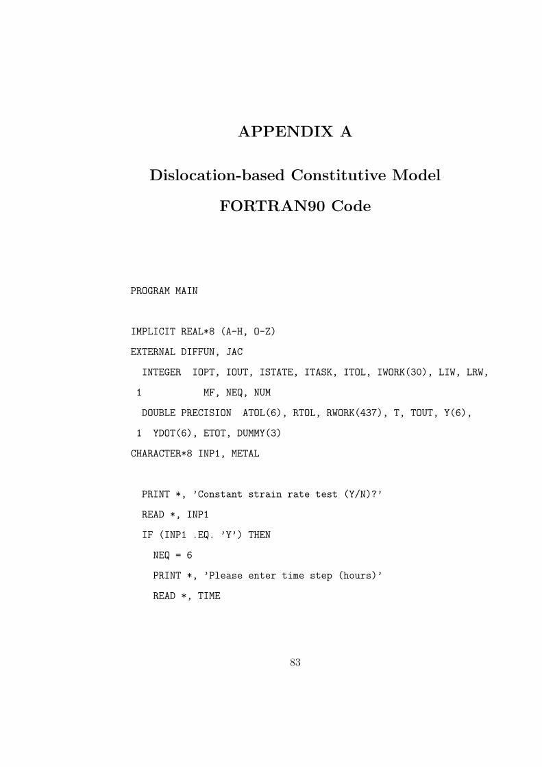
APPENDIX A

Dislocation-based Constitutive Model

FORTRAN90 Code

PROGRAM MAIN

IMPLICIT REAL*8 (A-H, O-Z)

EXTERNAL DIFFUN, JAC

INTEGER IOPT, IOUT, ISTATE, ITASK, ITOL, IWORK(30), LIW, LRW,

1 MF, NEQ, NUM

DOUBLE PRECISION ATOL(6), RTOL, RWORK(437), T, TOUT, Y(6),

1 YDOT(6), ETOT, DUMMY(3)

CHARACTER*8 INP1, METAL

PRINT *, ’Constant strain rate test (Y/N)?’

READ *, INP1

IF (INP1 .EQ. ’Y’) THEN

NEQ = 6

PRINT *, ’Please enter time step (hours)’

READ *, TIME

83

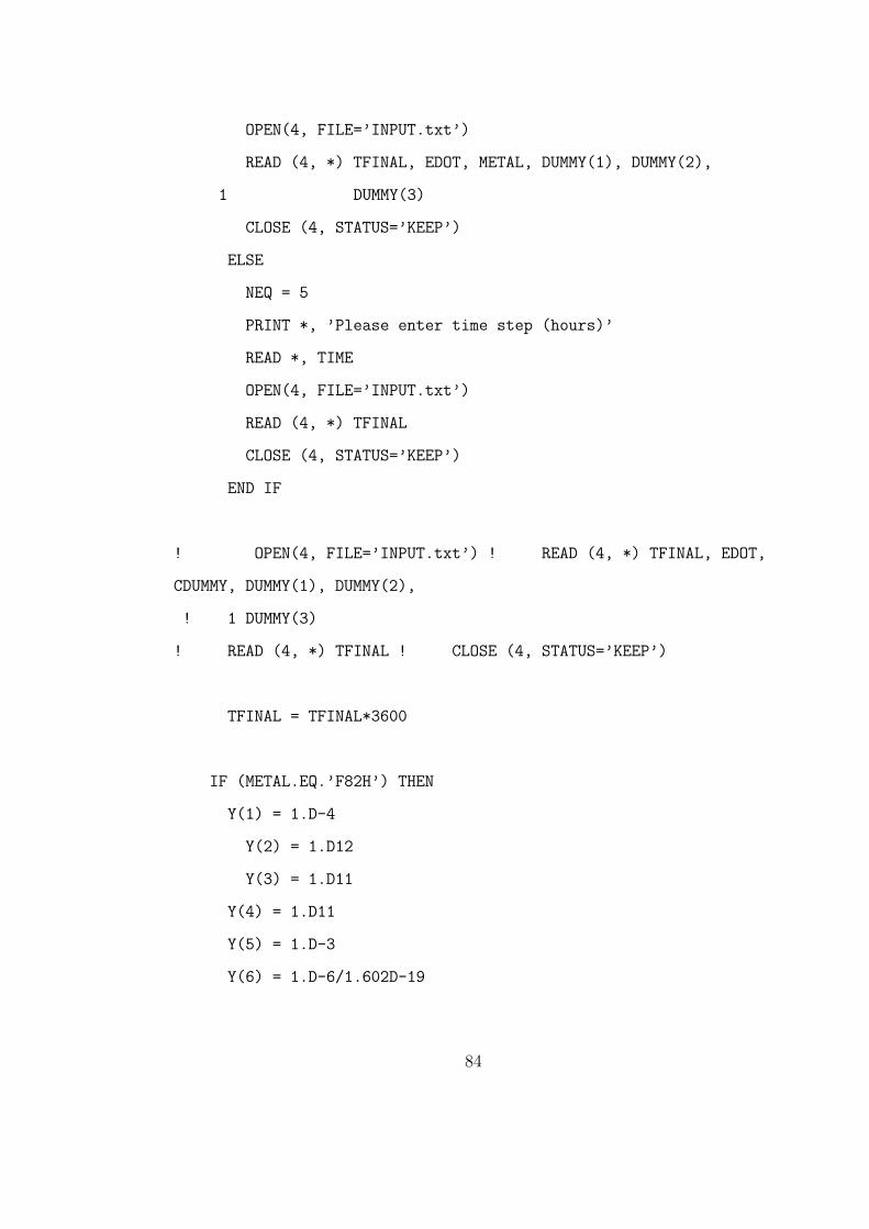
OPEN(4, FILE=’INPUT.txt’)

READ (4, *) TFINAL, EDOT, METAL, DUMMY(1), DUMMY(2),

1 DUMMY(3)

CLOSE (4, STATUS=’KEEP’)

ELSE

NEQ = 5

PRINT *, ’Please enter time step (hours)’

READ *, TIME

OPEN(4, FILE=’INPUT.txt’)

READ (4, *) TFINAL

CLOSE (4, STATUS=’KEEP’)

END IF

! OPEN(4, FILE=’INPUT.txt’) ! READ (4, *) TFINAL, EDOT,

CDUMMY, DUMMY(1), DUMMY(2),

! 1 DUMMY(3)

! READ (4, *) TFINAL ! CLOSE (4, STATUS=’KEEP’)

TFINAL = TFINAL*3600

IF (METAL.EQ.’F82H’) THEN

Y(1) = 1.D-4

Y(2) = 1.D12

Y(3) = 1.D11

Y(4) = 1.D11

Y(5) = 1.D-3

Y(6) = 1.D-6/1.602D-19

84

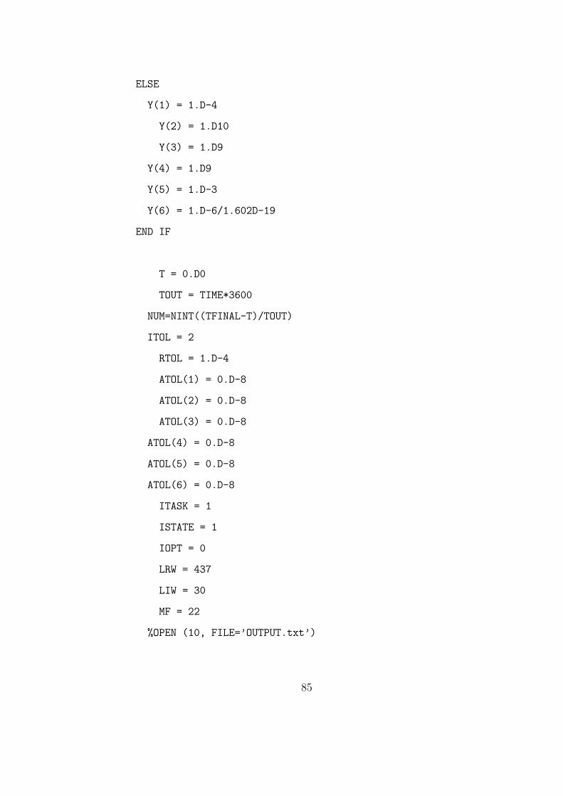
ELSE

Y(1) = 1.D-4

Y(2) = 1.D10

Y(3) = 1.D9

Y(4) = 1.D9

Y(5) = 1.D-3

Y(6) = 1.D-6/1.602D-19

END IF

T = 0.D0

TOUT = TIME*3600

NUM=NINT((TFINAL-T)/TOUT)

ITOL = 2

RTOL = 1.D-4

ATOL(1) = 0.D-8

ATOL(2) = 0.D-8

ATOL(3) = 0.D-8

ATOL(4) = 0.D-8

ATOL(5) = 0.D-8

ATOL(6) = 0.D-8

ITASK = 1

ISTATE = 1

IOPT = 0

LRW = 437

LIW = 30

MF = 22

%OPEN (10, FILE=’OUTPUT.txt’)

85

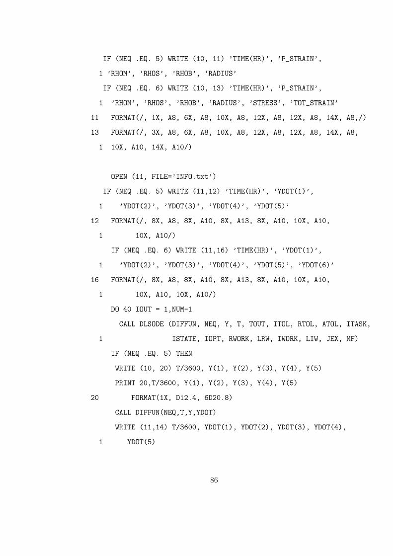
IF (NEQ .EQ. 5) WRITE (10, 11) ’TIME(HR)’, ’P_STRAIN’,

1 ’RHOM’, ’RHOS’, ’RHOB’, ’RADIUS’

IF (NEQ .EQ. 6) WRITE (10, 13) ’TIME(HR)’, ’P_STRAIN’,

1 ’RHOM’, ’RHOS’, ’RHOB’, ’RADIUS’, ’STRESS’, ’TOT_STRAIN’

11 FORMAT(/, 1X, A8, 6X, A8, 10X, A8, 12X, A8, 12X, A8, 14X, A8,/)

13 FORMAT(/, 3X, A8, 6X, A8, 10X, A8, 12X, A8, 12X, A8, 14X, A8,

1 10X, A10, 14X, A10/)

OPEN (11, FILE=’INFO.txt’)

IF (NEQ .EQ. 5) WRITE (11,12) ’TIME(HR)’, ’YDOT(1)’,

1 ’YDOT(2)’, ’YDOT(3)’, ’YDOT(4)’, ’YDOT(5)’

12 FORMAT(/, 8X, A8, 8X, A10, 8X, A13, 8X, A10, 10X, A10,

1 10X, A10/)

IF (NEQ .EQ. 6) WRITE (11,16) ’TIME(HR)’, ’YDOT(1)’,

1 ’YDOT(2)’, ’YDOT(3)’, ’YDOT(4)’, ’YDOT(5)’, ’YDOT(6)’

16 FORMAT(/, 8X, A8, 8X, A10, 8X, A13, 8X, A10, 10X, A10,

1 10X, A10, 10X, A10/)

DO 40 IOUT = 1,NUM-1

CALL DLSODE (DIFFUN, NEQ, Y, T, TOUT, ITOL, RTOL, ATOL, ITASK,

1 ISTATE, IOPT, RWORK, LRW, IWORK, LIW, JEX, MF)

IF (NEQ .EQ. 5) THEN

WRITE (10, 20) T/3600, Y(1), Y(2), Y(3), Y(4), Y(5)

PRINT 20,T/3600, Y(1), Y(2), Y(3), Y(4), Y(5)

20 FORMAT(1X, D12.4, 6D20.8)

CALL DIFFUN(NEQ,T,Y,YDOT)

WRITE (11,14) T/3600, YDOT(1), YDOT(2), YDOT(3), YDOT(4),

1 YDOT(5)

86

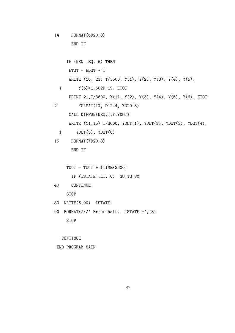
14 FORMAT(6D20.8)

END IF


ETOT = EDOT * T

WRITE (10, 21) T/3600, Y(1), Y(2), Y(3), Y(4), Y(5),

1 Y(6)*1.602D-19, ETOT

PRINT 21,T/3600, Y(1), Y(2), Y(3), Y(4), Y(5), Y(6), ETOT

21 FORMAT(1X, D12.4, 7D20.8)

CALL DIFFUN(NEQ,T,Y,YDOT)

WRITE (11,15) T/3600, YDOT(1), YDOT(2), YDOT(3), YDOT(4),

1 YDOT(5), YDOT(6)

15 FORMAT(7D20.8)

END IF

TOUT = TOUT + (TIME*3600)

IF (ISTATE .LT. 0) GO TO 80

40 CONTINUE

STOP

80 WRITE(6,90) ISTATE

90 FORMAT(///’ Error halt.. ISTATE =’,I3)

STOP

CONTINUE

END PROGRAM MAIN

87

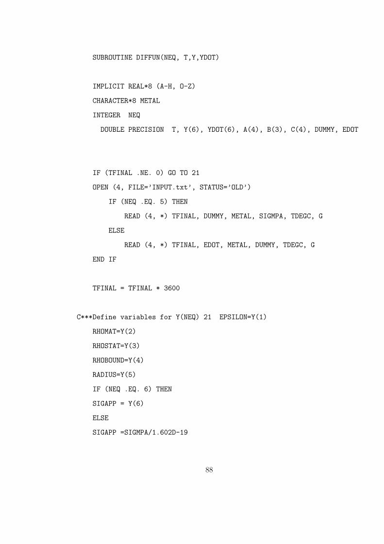
SUBROUTINE DIFFUN(NEQ, T,Y,YDOT)

IMPLICIT REAL*8 (A-H, O-Z)

CHARACTER*8 METAL

INTEGER NEQ

DOUBLE PRECISION T, Y(6), YDOT(6), A(4), B(3), C(4), DUMMY, EDOT

IF (TFINAL .NE. 0) GO TO 21

OPEN (4, FILE=’INPUT.txt’, STATUS=’OLD’)


READ (4, *) TFINAL, DUMMY, METAL, SIGMPA, TDEGC, G

ELSE

READ (4, *) TFINAL, EDOT, METAL, DUMMY, TDEGC, G

END IF

TFINAL = TFINAL * 3600

C***Define variables for Y(NEQ) 21 EPSILON=Y(1)

RHOMAT=Y(2)

RHOSTAT=Y(3)

RHOBOUND=Y(4)

RADIUS=Y(5)


SIGAPP = Y(6)

ELSE

SIGAPP =SIGMPA/1.602D-19

88

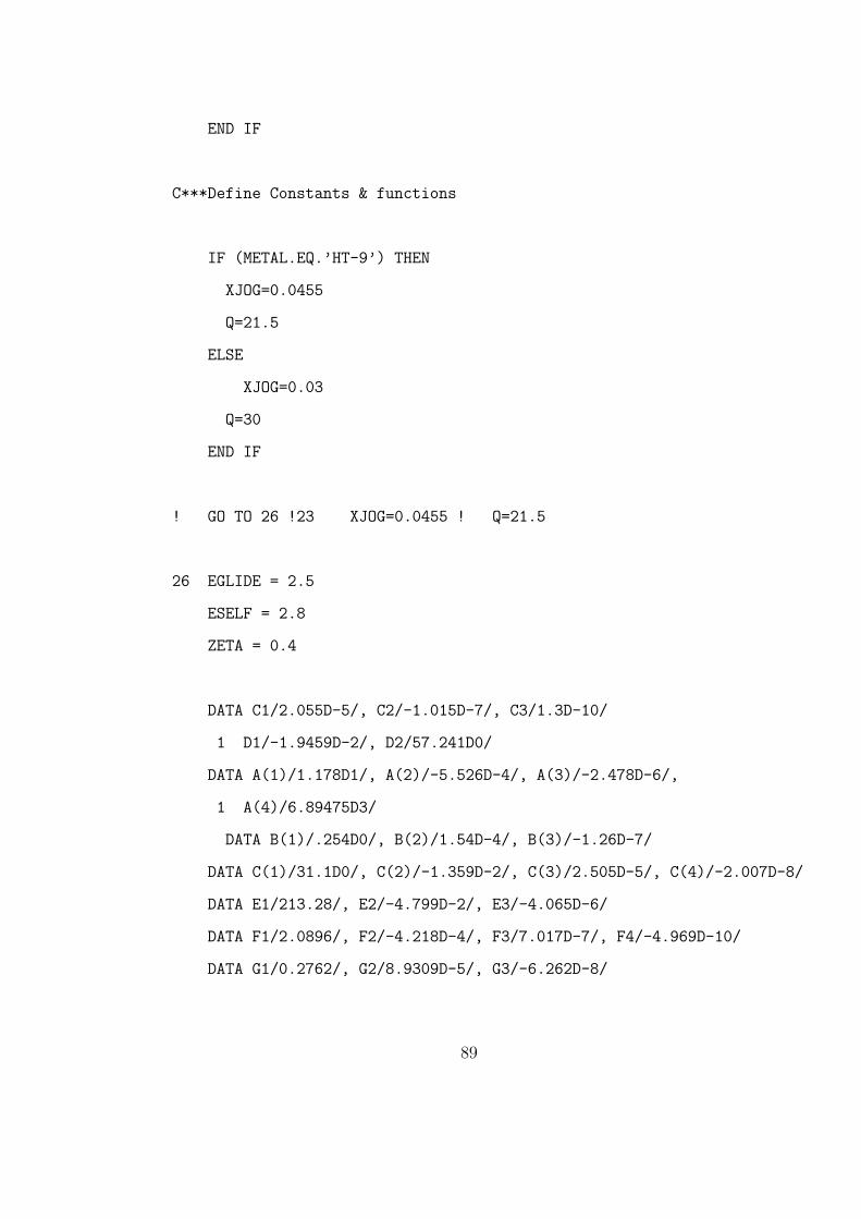
END IF

C***Define Constants & functions

IF (METAL.EQ.’HT-9’) THEN

XJOG=0.0455

Q=21.5

ELSE

XJOG=0.03

Q=30

END IF

! GO TO 26 !23 XJOG=0.0455 ! Q=21.5

26 EGLIDE = 2.5

ESELF = 2.8

ZETA = 0.4

DATA C1/2.055D-5/, C2/-1.015D-7/, C3/1.3D-10/

1 D1/-1.9459D-2/, D2/57.241D0/

DATA A(1)/1.178D1/, A(2)/-5.526D-4/, A(3)/-2.478D-6/,

1 A(4)/6.89475D3/

DATA B(1)/.254D0/, B(2)/1.54D-4/, B(3)/-1.26D-7/

DATA C(1)/31.1D0/, C(2)/-1.359D-2/, C(3)/2.505D-5/, C(4)/-2.007D-8/

DATA E1/213.28/, E2/-4.799D-2/, E3/-4.065D-6/

DATA F1/2.0896/, F2/-4.218D-4/, F3/7.017D-7/, F4/-4.969D-10/

DATA G1/0.2762/, G2/8.9309D-5/, G3/-6.262D-8/

89

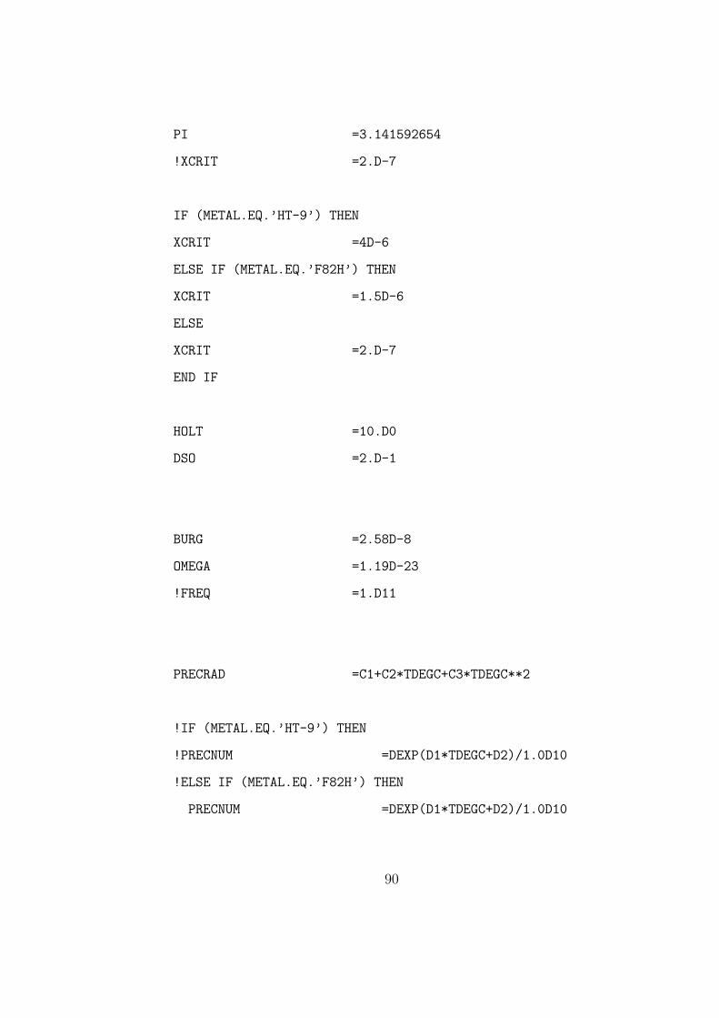
PI =3.141592654

!XCRIT =2.D-7


XCRIT =4D-6

ELSE IF (METAL.EQ.’F82H’) THEN

XCRIT =1.5D-6

ELSE

XCRIT =2.D-7

END IF

HOLT =10.D0

DSO =2.D-1

BURG =2.58D-8

OMEGA =1.19D-23

!FREQ =1.D11

PRECRAD =C1+C2*TDEGC+C3*TDEGC**2

!IF (METAL.EQ.’HT-9’) THEN

!PRECNUM =DEXP(D1*TDEGC+D2)/1.0D10

!ELSE IF (METAL.EQ.’F82H’) THEN

PRECNUM =DEXP(D1*TDEGC+D2)/1.0D10

90

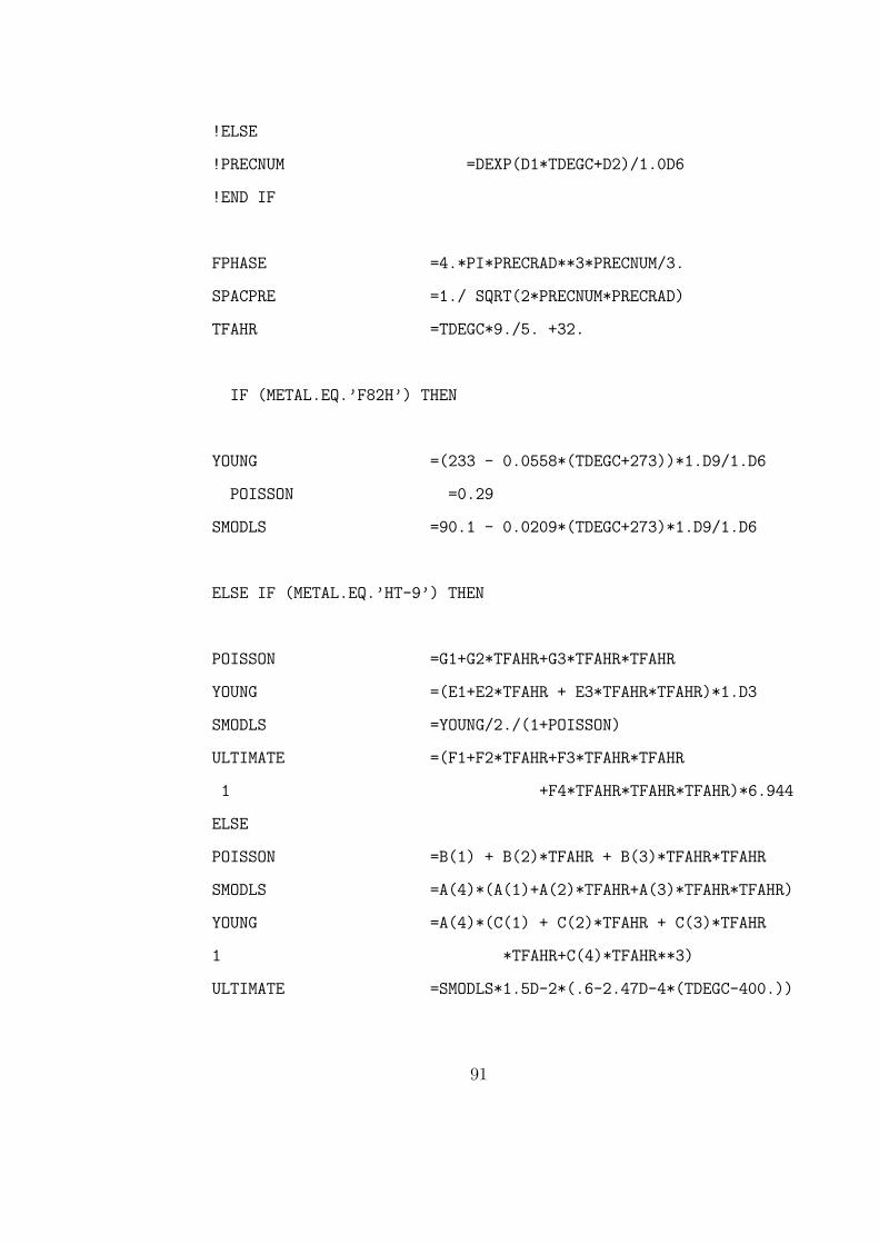
!ELSE

!PRECNUM =DEXP(D1*TDEGC+D2)/1.0D6

!END IF

FPHASE =4.*PI*PRECRAD**3*PRECNUM/3.

SPACPRE =1./ SQRT(2*PRECNUM*PRECRAD)

TFAHR =TDEGC*9./5. +32.

IF (METAL.EQ.’F82H’) THEN

YOUNG =(233 - 0.0558*(TDEGC+273))*1.D9/1.D6

POISSON =0.29

SMODLS =90.1 - 0.0209*(TDEGC+273)*1.D9/1.D6

ELSE IF (METAL.EQ.’HT-9’) THEN

POISSON =G1+G2*TFAHR+G3*TFAHR*TFAHR

YOUNG =(E1+E2*TFAHR + E3*TFAHR*TFAHR)*1.D3

SMODLS =YOUNG/2./(1+POISSON)

ULTIMATE =(F1+F2*TFAHR+F3*TFAHR*TFAHR

1 +F4*TFAHR*TFAHR*TFAHR)*6.944

ELSE

POISSON =B(1) + B(2)*TFAHR + B(3)*TFAHR*TFAHR

SMODLS =A(4)*(A(1)+A(2)*TFAHR+A(3)*TFAHR*TFAHR)

YOUNG =A(4)*(C(1) + C(2)*TFAHR + C(3)*TFAHR

1 *TFAHR+C(4)*TFAHR**3)

ULTIMATE =SMODLS*1.5D-2*(.6-2.47D-4*(TDEGC-400.))

91

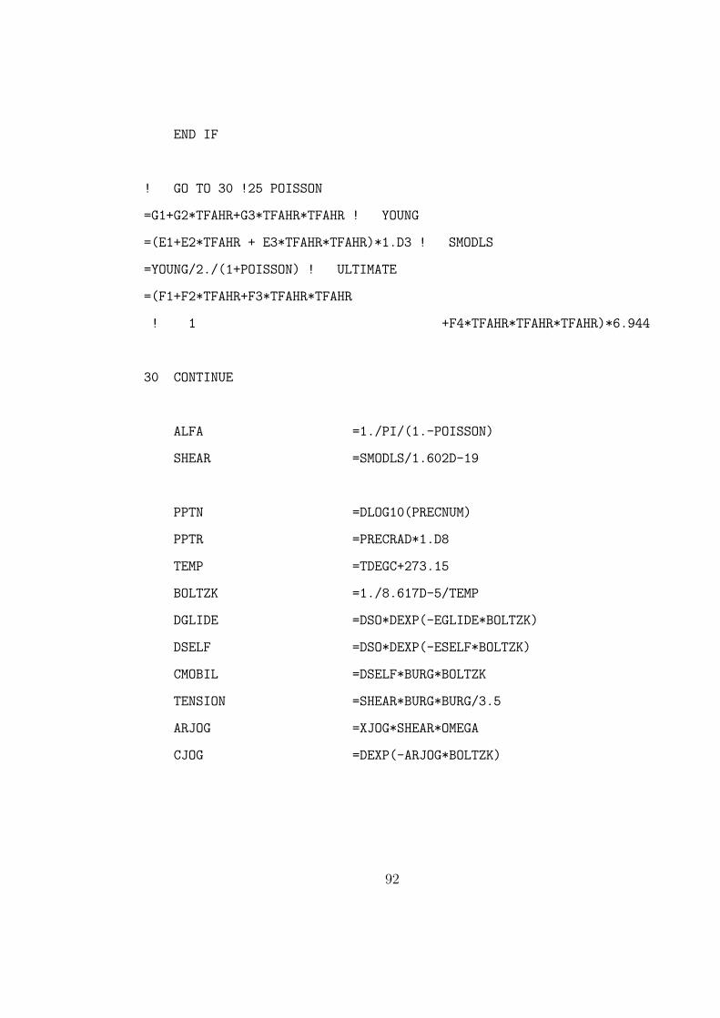
END IF

! GO TO 30 !25 POISSON

=G1+G2*TFAHR+G3*TFAHR*TFAHR ! YOUNG

=(E1+E2*TFAHR + E3*TFAHR*TFAHR)*1.D3 ! SMODLS

=YOUNG/2./(1+POISSON) ! ULTIMATE

=(F1+F2*TFAHR+F3*TFAHR*TFAHR

! 1 +F4*TFAHR*TFAHR*TFAHR)*6.944

30 CONTINUE

ALFA =1./PI/(1.-POISSON)

SHEAR =SMODLS/1.602D-19

PPTN =DLOG10(PRECNUM)

PPTR =PRECRAD*1.D8

TEMP =TDEGC+273.15

BOLTZK =1./8.617D-5/TEMP

DGLIDE =DSO*DEXP(-EGLIDE*BOLTZK)

DSELF =DSO*DEXP(-ESELF*BOLTZK)

CMOBIL =DSELF*BURG*BOLTZK

TENSION =SHEAR*BURG*BURG/3.5

ARJOG =XJOG*SHEAR*OMEGA

CJOG =DEXP(-ARJOG*BOLTZK)

92

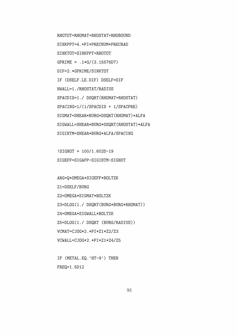
RHOTOT=RHOMAT+RHOSTAT+RHOBOUND

SINKPPT=4.*PI*PRECNUM*PRECRAD

SINKTOT=SINKPPT+RHOTOT

GPRIME = .1*G/(3.15576D7)

DIF=2.*GPRIME/SINKTOT

IF (DSELF.LE.DIF) DSELF=DIF

HWALL=1./RHOSTAT/RADIUS

SPACDIS=1./ DSQRT(RHOMAT+RHOSTAT)

SPACING=1/(1/SPACDIS + 1/SPACPRE)

SIGMAT=SHEAR*BURG*DSQRT(RHOMAT)*ALFA

SIGWALL=SHEAR*BURG*DSQRT(RHOSTAT)*ALFA

SIGINTM=SHEAR*BURG*ALFA/SPACING

!SIGNOT = 100/1.602D-19

SIGEFF=SIGAPP-SIGINTM-SIGNOT

ARG=Q*OMEGA*SIGEFF*BOLTZK

Z1=DSELF/BURG

Z2=OMEGA*SIGMAT*BOLTZK

Z3=DLOG(1./ DSQRT(BURG*BURG*RHOMAT))

Z4=OMEGA*SIGWALL*BOLTZK

Z5=DLOG(1./ DSQRT (BURG/RADIUS))

VCMAT=CJOG*2.*PI*Z1*Z2/Z3

VCWALL=CJOG*2.*PI*Z1*Z4/Z5


FREQ=1.5D12

93

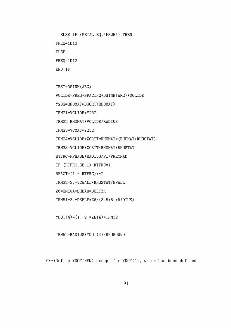
ELSE IF (METAL.EQ.’F82H’) THEN

FREQ=1D13

ELSE

FREQ=1D12

END IF

TEST=DSINH(ARG)

VGLIDE=FREQ*SPACING*DSINH(ARG)*DGLIDE

Y232=RHOMAT*DSQRT(RHOMAT)

TRM21=VGLIDE*Y232

TRM22=RHOMAT*VGLIDE/RADIUS

TRM23=VCMAT*Y232

TRM24=VGLIDE*XCRIT*RHOMAT*(RHOMAT+RHOSTAT)

TRM33=VGLIDE*XCRIT*RHOMAT*RHOSTAT

RTFRC=FPHASE*RADIUS/PI/PRECRAD

IF (RTFRC.GE.1) RTFRC=1.

RFACT=(1.- RTFRC)**2

TRM32=2.*VCWALL*RHOSTAT/HWALL

Z6=OMEGA*SHEAR*BOLTZK

TRM51=3.*DSELF*Z6/(3.5*8.*RADIUS)

YDOT(4)=(1.-2.*ZETA)*TRM32

TRM52=RADIUS*YDOT(4)/RHOBOUND

C***Define YDOT(NEQ) except for YDOT(4), which has been defined

94

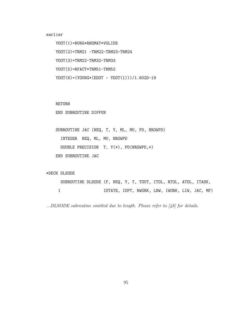
earlier

YDOT(1)=BURG*RHOMAT*VGLIDE

YDOT(2)=TRM21 -TRM22-TRM23-TRM24

YDOT(3)=TRM22-TRM32-TRM33

YDOT(5)=RFACT*TRM51-TRM52

YDOT(6)=(YOUNG*(EDOT - YDOT(1)))/1.602D-19

RETURN

END SUBROUTINE DIFFUN

SUBROUTINE JAC (NEQ, T, Y, ML, MU, PD, NROWPD)

INTEGER NEQ, ML, MU, NROWPD

DOUBLE PRECISION T, Y(*), PD(NROWPD,*)

END SUBROUTINE JAC

*DECK DLSODE

SUBROUTINE DLSODE (F, NEQ, Y, T, TOUT, ITOL, RTOL, ATOL, ITASK,

1 ISTATE, IOPT, RWORK, LRW, IWORK, LIW, JAC, MF)

...DLSODE subroutine omitted due to length. Please refer to [48] for details.

95

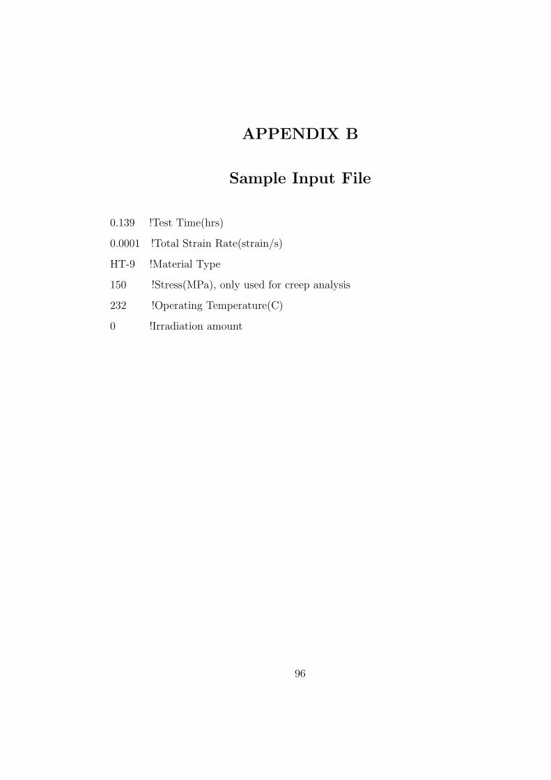
APPENDIX B

Sample Input File

0.139 !Test Time(hrs)

0.0001 !Total Strain Rate(strain/s)

HT-9 !Material Type

150 !Stress(MPa), only used for creep analysis

232 !Operating Temperature(C)

0 !Irradiation amount

96

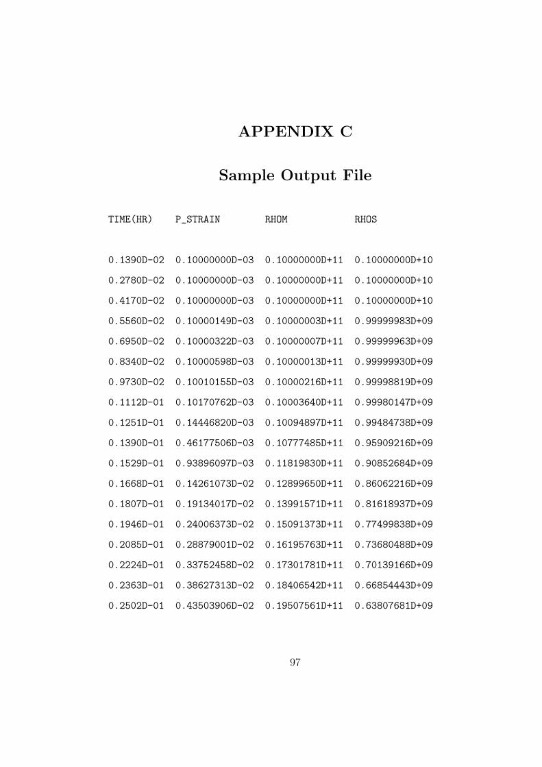
APPENDIX C

Sample Output File

TIME(HR) P_STRAIN RHOM RHOS

0.1390D-02 0.10000000D-03 0.10000000D+11 0.10000000D+10

0.2780D-02 0.10000000D-03 0.10000000D+11 0.10000000D+10

0.4170D-02 0.10000000D-03 0.10000000D+11 0.10000000D+10

0.5560D-02 0.10000149D-03 0.10000003D+11 0.99999983D+09

0.6950D-02 0.10000322D-03 0.10000007D+11 0.99999963D+09

0.8340D-02 0.10000598D-03 0.10000013D+11 0.99999930D+09

0.9730D-02 0.10010155D-03 0.10000216D+11 0.99998819D+09

0.1112D-01 0.10170762D-03 0.10003640D+11 0.99980147D+09

0.1251D-01 0.14446820D-03 0.10094897D+11 0.99484738D+09

0.1390D-01 0.46177506D-03 0.10777485D+11 0.95909216D+09

0.1529D-01 0.93896097D-03 0.11819830D+11 0.90852684D+09

0.1668D-01 0.14261073D-02 0.12899650D+11 0.86062216D+09

0.1807D-01 0.19134017D-02 0.13991571D+11 0.81618937D+09

0.1946D-01 0.24006373D-02 0.15091373D+11 0.77499838D+09

0.2085D-01 0.28879001D-02 0.16195763D+11 0.73680488D+09

0.2224D-01 0.33752458D-02 0.17301781D+11 0.70139166D+09

0.2363D-01 0.38627313D-02 0.18406542D+11 0.66854443D+09

0.2502D-01 0.43503906D-02 0.19507561D+11 0.63807681D+09

97

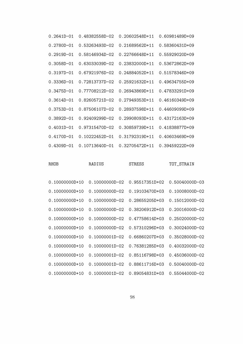
0.2641D-01 0.48382558D-02 0.20602548D+11 0.60981489D+09

0.2780D-01 0.53263493D-02 0.21689562D+11 0.58360431D+09

0.2919D-01 0.58146934D-02 0.22766648D+11 0.55929020D+09

0.3058D-01 0.63033039D-02 0.23832000D+11 0.53672862D+09

0.3197D-01 0.67921976D-02 0.24884052D+11 0.51578346D+09

0.3336D-01 0.72813737D-02 0.25921632D+11 0.49634755D+09

0.3475D-01 0.77708212D-02 0.26943869D+11 0.47833291D+09

0.3614D-01 0.82605721D-02 0.27949353D+11 0.46160349D+09

0.3753D-01 0.87506107D-02 0.28937598D+11 0.44609099D+09

0.3892D-01 0.92409299D-02 0.29908093D+11 0.43172163D+09

0.4031D-01 0.97315470D-02 0.30859739D+11 0.41838877D+09

0.4170D-01 0.10222452D-01 0.31792319D+11 0.40603469D+09

0.4309D-01 0.10713640D-01 0.32705472D+11 0.39459222D+09

RHOB RADIUS STRESS TOT_STRAIN

0.10000000D+10 0.10000000D-02 0.95517351D+02 0.50040000D-03

0.10000000D+10 0.10000000D-02 0.19103470D+03 0.10008000D-02

0.10000000D+10 0.10000000D-02 0.28655205D+03 0.15012000D-02

0.10000000D+10 0.10000000D-02 0.38206912D+03 0.20016000D-02

0.10000000D+10 0.10000000D-02 0.47758614D+03 0.25020000D-02

0.10000000D+10 0.10000000D-02 0.57310296D+03 0.30024000D-02

0.10000000D+10 0.10000001D-02 0.66860207D+03 0.35028000D-02

0.10000000D+10 0.10000001D-02 0.76381285D+03 0.40032000D-02

0.10000000D+10 0.10000001D-02 0.85116798D+03 0.45036000D-02

0.10000000D+10 0.10000001D-02 0.88611716D+03 0.50040000D-02

0.10000000D+10 0.10000001D-02 0.89054831D+03 0.55044000D-02

98

0.10000000D+10 0.10000001D-02 0.89307819D+03 0.60048000D-02

0.10000000D+10 0.10000001D-02 0.89557983D+03 0.65052000D-02

0.10000000D+10 0.10000001D-02 0.89809267D+03 0.70056000D-02

0.10000000D+10 0.10000001D-02 0.90060031D+03 0.75060000D-02

0.10000000D+10 0.10000001D-02 0.90309215D+03 0.80064000D-02

0.10000000D+10 0.10000001D-02 0.90555731D+03 0.85068000D-02

0.10000000D+10 0.10000001D-02 0.90798928D+03 0.90072000D-02

0.10000000D+10 0.10000001D-02 0.91038194D+03 0.95076000D-02

0.10000000D+10 0.10000001D-02 0.91273103D+03 0.10008000D-01

0.10000000D+10 0.10000001D-02 0.91503228D+03 0.10508400D-01

0.10000000D+10 0.10000001D-02 0.91728269D+03 0.11008800D-01

0.10000000D+10 0.10000001D-02 0.91947902D+03 0.11509200D-01

0.10000000D+10 0.10000001D-02 0.92162147D+03 0.12009600D-01

0.10000000D+10 0.10000001D-02 0.92371211D+03 0.12510000D-01

0.10000000D+10 0.10000001D-02 0.92574482D+03 0.13010400D-01

0.10000000D+10 0.10000001D-02 0.92772263D+03 0.13510800D-01

0.10000000D+10 0.10000001D-02 0.92964687D+03 0.14011200D-01

0.10000000D+10 0.10000001D-02 0.93151426D+03 0.14511600D-01

0.10000000D+10 0.10000001D-02 0.93332674D+03 0.15012000D-01

0.10000000D+10 0.10000001D-02 0.93508503D+03 0.15512400D-01

99

References

[1] R. J. Amodeo and N. M. Ghoniem. Constitutive design equations for thermalcreep deformation of ht-9, ppg-743. University of California Report, 1983.

[2] A. S. Argon and W. Moffatt. Acta Metallurgica, 29:293, 1981.

[3] M. F. Ashby. The influence of particles on boundary mobility. Proc. 1stRiso Int. Symp. on Metallurgy and Materials Science Recrystallisation andGrain Growth of Multi-Phase and Particle Containing Materials., 1980.

[4] S. Mader H Rebstock A. Seeger, J. Diehl. Work-hardening and work-softening of face-centred cubic metal crystals. Phil Mag, 2:323, 1957.

[5] P. Haasen A. S. Argon. A new mechanism of work hardening in the latestages of large strain plastic flow in f.c.c and diamond cubic crystals. ActaMetallurgica, 41:3289–3306, 1993.

[6] Z. S. Basinski. Thermally activated glide in face-centred cubic metals andits application to the theory of strain hardening. Phil Mag, 4:393, 1959.

[7] Y. Bergstrom. A dislocation model for the stress-strain behavior of polycrys-talline α-fe with special emphasis on the variation of the densities of mobileand immobile dislocations. Materials Science and Engineering, 5:193, 1970.

[8] R. Bullough and J. R. Willis. Philosophical Magazine, 31:855, 1975.

[9] K. D. Challenger and J. Moteff. Metall Trans, 4:749, 1973.

[10] A. H. Cottrell. Prog. Metall. Physics, 1:77, 1952.

[11] A. H. Cottrell. Dislocations and Plastic Flow in Crystals. Oxfored at theClarendon Press, 1953.

[12] I. J. Cuddy. Metall Trans, 1:395, 1970.

[13] J. Moteff D. J. Michel and A. J. Lovell. Acta Metallurgica, 21:1269, 1973.

[14] U. Essmann and H. Mughrabi. Annihilation of dislocations during tensileand cyclic deformation and limits of dislocation densities.

[15] Y. Estrin and H. Mecking. A unified phenomenological description of workhardening and creep based on one-parameter models. Acta Metallurgica,32:57–70, 1984.

100

[16] Y. Estrin. Dislocation theory based constitutive modelling: foundations andapplications. Materials Processing Technology, 80-81:33–39, 1998.

[17] H. E. Evans and G. Knowles. Acta Metallurgica, 25:963, 1977.

[18] J. Friedel. Dislocations. Addison-Wesley Publishing Compan, Inc., 1964.

[19] A. S. Argon F. B. Prinz. The evolution of plastic resistance in large strainplastic flow of single phase subgrain forming metals. Acta Metallurgica,32:1021–1028, 1984.

[20] D. Raabe F. Roters and G. Gottstein. Work hardening in heterogeneousalloys-a microstrutural approach based on three internal state variables.Acta Materialia, 48:4181–4189, 2000.

[21] N. M. Ghoniem and R. J. Amodeo. Sol. State Phenom., 3 and 4:377, 1988.

[22] N. M. Ghoniem and K. Cho. The emerging role of multiscale modeling innano- and micro-mechanics of materials. J. Comp. Meth. Engr. Science,3(2):147–173, 2002.

[23] J. H. Gittus. Multiaxial mechanical equation of states for a work-hardening/recovery model of dislocation creep. Philosophical Magazine,25:1233, 1972.

[24] J. H. Gittus. Philosophical Magazine, 35:293, 1977.

[25] J. H. Gittus. Philosophical Magazine, 39:829, 1979.

[26] J. Gittus. The mechanical equation of states: Disloction creep due to stressesvarying in magnitude and direction. Philosophical Magazine, pages 1423–1440, 1971.

[27] A.S Argon G. Gottstein. Dislocation theory of steady state deformation andits approach in creep and dynamic tests. Acta Metallurgica, 35:1261–1271,1987.

[28] P. T. Heald and M. V. Speight. Philosophical Magazine, 29:1075, 1974.

[29] D. Holt. Journal of Applied Physics, 41:3197, 1970.

[30] Hull. Introduction to Dislocation. Pergamon Press Ltd., 1969.

[31] U.F. Kocks H. Mecking. Kinetics of flow and strain-hardening. Acta Metal-lurgica, 29:1865–1875, 1981.

101

[32] ANSYS Inc. Ansys 7.1 documentation. 2003.

[33] T.J.R Hughes J.C. Simo. Computational Inelasticity. Springer, 1998.

[34] W. G. Johnson and J. J. Gilman. Journal of Applied Physics, 30:129, 1950.

[35] R. D. Martinez Jr. The influence of crystal surfaces on dislocation behaviorin mesoscopic plasticity: A combined dislocation dynamics-finite elementapproach. Master’s thesis, University of California, Los Angeles, 2000.

[36] J. Lothe J. P. Hirth. Theory of Dislocations. John Wiley and Sons, Inc.,1982.

[37] K.Domkin. A brief review of physically based material models. 2001.

[38] U. F. Kocks. A statistical theory of flow stress and work-hardening. PhilMag, 13:541, 1966.

[39] T. G. Langdon. Dislocations and creep. Proc. Conf. on Dislocations and theProperties of Real Materials, Royal Society of London, page 221, 1984.

[40] J. C. M. Li. Journal of Applied Physics, 33(10), 1962.

[41] A. Mendelson. PLASTICITY: theory and application. Robert E. KriegerPublishing Company, Inc., 1968.

[42] H. Mughrabi. A two-parameter description of heterogeneous dislocation dis-tributions in deformed metal crystals. Materials Science and Engineering,85:15–31, 1987.

[43] H. Mughrabi. Dislocation clustering and long-range internal stresses inmonotonically and cyclically deformed metal crystals. Revue Phys Appl,23:367–379, 1988.

[44] W. Blum M. Meier. Modelling high temperature creep of academic andindustrial meterials using the composite model. Materials Science and En-gineering, A164:290–294, 1993.

[45] F. R. N. Nabarro. Steady-state diffusional creep. Philosophical Magazine,page 231, 1967.

[46] N. Kioussis N. M. Ghoniem, E. P. Busso and H. Huang. Multiscale mod-elling of nanomechanics and micromechanics: an overview. PhilosophicalMagazine, received 4 June 2003, 2003.

102

[47] R. J. Amodeo N. M. Ghoniem, J. R. Matthews. A dislocation model forcreep in engineering materials. Res Mechanica, 29:197–219, 1990.

[48] K. Radhakrishnan and A. C. Hindmarsh. Description and use of lsode, thelivermore solver for ordinary differential equations. LLNL report UCRL-ID-113855, 1993.

[49] H. Rauh and R. Bullough. Philosophical Magazine, 52:33, 1985.

[50] M. W. Finnis R. Bullough and M. H. Wood. Journal of Nuclear Materials,103:1263, 1981.

[51] B. H. Forsen R. Lagneborg and J. Wiberg. A recovery-creep model basedupon dislocation distributions. The Materials Society, London, pages 1–7,1974.

[52] W. Blum R. Sedlacek. Microstructure-based constitutve law of plastic de-formation. Computational Materials Science, 25:200–206, 2002.

[53] Rolf Sandstrom. On recovery of dislocations in subgrains and subgrain coa-lescence. Acta Metallurgica, 25:897–904, 1977.

[54] Rolf Sandstrom. Subgrain growth occuring by boundary migration. ActaMetallurgica, 25:905–911, 1977.

[55] J. P. Robertson S. J. Zinkle and R. J. Klueh. Thermophysical and mechanicalproperties of fe-(8-9)activation steel. Oakridge National Lab, 1998.

[56] A. S. Argon S. Takeuchi. Steady-state creep of single-phase crystalline mat-ter at high temperature. Journal of Applied Materials Science, 11:1542–1566, 1976.

[57] A. S. Argon S. Takeuchi. Stead-state creep of alloys due to viscous motionof dislocations. Acta Metallurgica, 24:883, 1976.

[58] W.L. Bell T. Lauritzen and S. Vaidyanathan. Effects of irradiation on themechanical properties of ferritic alloys ht-9 and 2.25r-1mo. Proceedings ofTopical Conference on Ferritic Alloys for use in Nuclear Energy Technolo-gies, pages 623–630, 1983.

[59] E. Voce. Inst Metals, 74:537, 1948.

[60] G. A. Webster. Philosophical Magazine, 14:775, 1966.

103

[61] Yngve Bergstrom William Roberts. The stress-strain behavior of single crys-tal and polycrystal of face-centered cubic metals-a new dislocation treat-ment. Acta Metallurgica, 21:457–469, 1973.

[62] A. Cegielska W. Blum, A. Rosen and J. L. Martin. Two mechanisms ofdislocation motion during creep. Acta Metallurgica, 37:2439–2453, 1989.

[63] S. Vogler W. Blum and M. Biberger. Stress dependence of the creep rate atconstant dislocation structure. Materials Science and Engineering, A112:93–106, 1989.

[64] Jr. W. T. Read. Dislocations in Crystals. McGraw-Hill Book Company,Inc., 1953.

[65] H. Hallen Y. Bergstrom. An improved dislocation model for the stress-strainbehavior of polycrystalline α-fe. Materials Science and Engineering, 55:49–61, 1982.

[66] Y. Brechet Y. Estrin, H. Braasch. A dislocation density based constitutivemodel for cyclic deformation. Journal of Engineering Materials and Tech-nology, 118:441, 1996.

[67] M.t L. Hamilton T. Hirose Y. Katoh Y. Kohno, A. Kohyama and F. A.Garner. Specimen size effects on the tensile properties of jpca and jfms.Journal of Nuclear Materials, 283-287.

[68] M. Zehetbauer. Cold work hardening in stages iv and v of f.c.c metals-ii.model fits and physical results. Acta Metallurgica, 41:589–599, 1993.

104

Dislocation-Based Finite Element Modelling of Elasto...

Documents

Transcript of Dislocation-Based Finite Element Modelling of Elasto...