Disentangling Bias and Variance in Election Polls

Houshmand Shirani-MehrStanford University

David RothschildMicrosoft Research

Sharad GoelStanford University

Andrew GelmanColumbia University

Abstract

It is well known among researchers and practitioners that election polls suffer from

a variety of sampling and non-sampling errors, often collectively referred to as total

survey error. Reported margins of error typically only capture sampling variability,

and in particular, generally ignore non-sampling errors in defining the target popula-

tion (e.g., errors due to uncertainty in who will vote). Here we empirically analyze

4,221 polls for 608 state-level presidential, senatorial, and gubernatorial elections be-

tween 1998 and 2014, all of which were conducted during the final three weeks of the

campaigns. Comparing to the actual election outcomes, we find that average survey

error as measured by root mean square error (RMSE) is approximately 3.5 percentage

points, about twice as large as that implied by most reported margins of error. We de-

compose survey error into election-level bias and variance terms, and find that average

absolute election-level bias is about 2.0 percentage points, indicating that polls for a

given election often share a common component of error. This shared error may stem

from the fact that polling organizations often face similar difficulties in reaching various

subgroups of the population, and they rely on similar screening rules when estimating

who will vote. Election-level bias accounts for much, but not all, the observed excess

error; as a result, average election-level variance is also higher than implied by most

reported margins of error. We conclude by discussing how these results help explain

polling failures in the 2016 U.S. presidential election, and offer recommendations to

improve polling practice.

1 Introduction

Election polling is arguably the most visible manifestation of statistics in everyday life,

and embodies one of the great success stories of statistics: random sampling. As is recounted

in so many textbooks, the huge but uncontrolled Literary Digest poll was trounced by

Gallup’s small, nimble random sample back in 1936. Election polls are a high-profile reality

check on statistical methods.

It has long been known that the margins of errors provided by survey organizations,

and reported in the news, understate the total survey error. This is an important topic in

sampling but is difficult to address in general for two reasons. First, we like to decompose

error into bias and variance, but this can only be done with any precision if we have a large

number of surveys and outcomes—not merely a large number of respondents in an individual

survey. Second, assessment of error requires a ground truth for comparison, which is typically

not available, as the reason for conducting a sample survey in the first place is to estimate

some population characteristic that is not already known.

In the present paper we decompose survey error in a large set of state-level pre-election

polls. This dataset resolves both of the problems just noted. First, the combination of

multiple elections and many states gives us a large sample of polls. Second, we can compare

the polls to actual election results.

1.1 Background

Election polls typically survey a random sample of eligible or likely voters, and then

generate population-level estimates by taking a weighted average of responses, where the

weights are designed to correct for known differences between sample and population.1 This

general analysis framework yields both a point estimate of the election outcome, and also an

estimate of the error in that prediction due to sample variance which accounts for the survey

1One common technique for setting survey weights is raking, in which weights are defined so that theweighted distributions of various demographic features (e.g., age, sex, and race) of respondents in the sampleagree with the marginal distributions in the target population [Voss, Gelman, and King, 1995].

2

weights [Lohr, 2009]. In practice, weights in a sample tend to be approximately equal, and so

most major polling organizations simply report 95% margins of error identical to those from

simple random sampling (SRS) without incorporating the effect of the weights, for example

±3.5 percentage points for an election survey with 800 people.2

Though this approach to quantifying polling error is popular and convenient, it is well

known by both researchers and practitioners that discrepancies between poll results and elec-

tion outcomes are only partially attributable to sample variance [Ansolabehere and Belin,

1993]. As observed in the extensive literature on total survey error [Biemer, 2010, Groves

and Lyberg, 2010], there are at least four additional types of error that are not reflected

in the usually reported margins of error: frame, nonresponse, measurement, and specifica-

tion. Frame error occurs when there is a mismatch between the sampling frame and the

target population. For example, for phone-based surveys, people without phones would

never be included in any sample. Of particular import for election surveys, the sampling

frame includes many adults who are not likely to vote, which pollsters recognize and at-

tempt to correct for using likely voters screens, typically estimated with error from survey

questions. Nonresponse error occurs when missing values are systematically related to the

response. For example, supporters of the trailing candidate may be less likely to respond

to surveys [Gelman, Goel, Rivers, and Rothschild, 2016]. With nonresponse rates exceeding

90% for election surveys, this is a growing concern [Pew Research Center, 2016]. Measure-

ment error arises when the survey instrument itself affects the response, for example due

to order effects [McFarland, 1981] or question wording [Smith, 1987]. Finally, specification

error occurs when a respondent’s interpretation of a question differs from what the surveyor

intends to convey (e.g., due to language barriers). In addition to these four types of error

2For the 19 ABC, CBS, and Gallup surveys conducted during the 2012 election and deposited into RoperCenter’s iPoll, when weights in each survey were rescaled to have mean 1, the median respondent weight was0.73, with an interquartile range of 0.45 to 1.28. For a sampling of 96 polls for 2012 Senate elections, only19 reported margins of error higher than what one would compute using the SRS formula, and 14 of theseexceptions were accounted for by YouGov, an internet poll that explicitly inflates variance to adjust for thesampling weights. Similarly, for a sampling of 36 state-level polls for the 2012 presidential election, only 9reported higher-than-SRS margins of error.

3

common to nearly all surveys, election polls suffer from an additional complication: shifting

attitudes. Whereas surveys typically seek to gauge what respondents will do on election day,

they can only directly measure current beliefs.

In contrast to errors due to sample variance, it is difficult—and perhaps impossible—to

build a useful and general statistical theory for the remaining components of total survey

error. Moreover, even empirically measuring total survey error can be difficult, as it involves

comparing the results of repeated surveys to a ground truth obtained, for example, via a

census. For these reasons, it is not surprising that many survey organizations continue to

use estimates of error based on theoretical sampling variation, simply acknowledging the

limitations of the approach. Indeed, Gallup [2007] explicitly states that their methodology

assumes “other sources of error, such as nonresponse, by some members of the targeted

sample are equal,” and further notes that “other errors that can affect survey validity include

measurement error associated with the questionnaire, such as translation issues and coverage

error, where a part or parts of the target population...have a zero probability of being selected

for the survey.”

1.2 Our study

Here we empirically and systematically study error in election polling, taking advantage

of the fact that multiple polls are typically conducted for each election, and that the election

outcome can be taken to be the ground truth. We investigate 4,221 polls for 608 state-level

presidential, senatorial, and gubernatorial elections between 1998 and 2014, all of which were

conducted in the final three weeks of the election campaigns. By focusing on the final weeks

of the campaigns, we seek to minimize the impact of errors due to changing attitudes in the

electorate, and hence to isolate the effects of the remaining components of survey error.

We find that the average difference between poll results and election outcomes—as mea-

sured by RMSE—is 3.5 percentage points, about twice the error implied by most reported

4

confidence intervals.3 To decompose this survey error into election-level bias and variance

terms, we carry out a Bayesian meta-analysis. We find that average absolute election-level

bias is about 2.0 percentage points, indicating that polls for a given election often share

a common component of error. This result is likely driven in part by the fact that most

polls, even when conducted by different polling organizations, rely on similar likely voter

models, and thus surprises in election day turnout can have comparable effects on all the

polls. Moreover, these correlated frame errors extend to the various elections—presidential,

senatorial, and gubernatorial—across the state.

2 Data

2.1 Data description

Our primary analysis is based on 4,221 polls completed during the final three weeks of

608 state-level presidential, senatorial, and gubernatorial elections between 1998 and 2014.

Polls are typically conducted over the course of several days, and following convention, we

throughout associate the “date” of the poll with the last date during which it was in the

field. We do not include House elections in our analysis since polling is only available for a

small and non-representative subset of such races.

To construct this dataset, we started with the 4,154 state-level polls for elections in

1998–2013 that were collected and made available by FiveThirtyEight, all of which were

completed during the final three weeks of the campaigns. We augment these polls with

the 67 corresponding ones for 2014 posted on Pollster.com, where for consistency with the

FiveThirtyEight data, we consider only those completed in the last three weeks of the cam-

paigns. In total, we end up with 1,646 polls for 241 senatorial elections, 1,496 polls for 179

3Most reported margins of error assume estimates are unbiased, and report 95% confidence intervals ofapproximately ±3.5 percentage points for a sample of 800 respondents. This in turn implies the RMSEfor such a sample is approximately 1.8 percentage points, approximately half of our empirical estimate ofRMSE.

5

state-level presidential elections, and 1,079 polls for 188 gubernatorial elections.

In addition to our primary dataset described above, we also consider 7,040 polls completed

during the last 100 days of 314 state-level presidential, senatorial, and gubernatorial elections

between 2004 and 2012. All polls for this secondary dataset were obtained from Pollster.com

and RealClearPolitics.com. Whereas this complementary set of polls covers only the more

recent elections, it has the advantage of containing polls conducted earlier in the campaign

cycle.

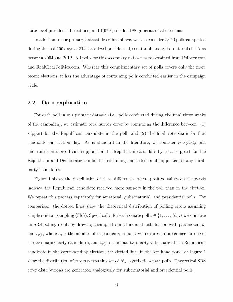
2.2 Data exploration

For each poll in our primary dataset (i.e., polls conducted during the final three weeks

of the campaign), we estimate total survey error by computing the difference between: (1)

support for the Republican candidate in the poll; and (2) the final vote share for that

candidate on election day. As is standard in the literature, we consider two-party poll

and vote share: we divide support for the Republican candidate by total support for the

Republican and Democratic candidates, excluding undecideds and supporters of any third-

party candidates.

Figure 1 shows the distribution of these differences, where positive values on the x-axis

indicate the Republican candidate received more support in the poll than in the election.

We repeat this process separately for senatorial, gubernatorial, and presidential polls. For

comparison, the dotted lines show the theoretical distribution of polling errors assuming

simple random sampling (SRS). Specifically, for each senate poll i ∈ {1, . . . , Nsen} we simulate

an SRS polling result by drawing a sample from a binomial distribution with parameters ni

and vr[i], where ni is the number of respondents in poll i who express a preference for one of

the two major-party candidates, and vr[i] is the final two-party vote share of the Republican

candidate in the corresponding election; the dotted lines in the left-hand panel of Figure 1

show the distribution of errors across this set of Nsen synthetic senate polls. Theoretical SRS

error distributions are generated analogously for gubernatorial and presidential polls.

6

Senatorial Gubernatorial Presidential

−10% −5% 0% 5% 10% −10% −5% 0% 5% 10% −10% −5% 0% 5% 10%

Difference between poll results and election outcomes

Figure 1: The distribution of polling errors (Republican share of two-party support in thepoll minus Republican share of the two-party vote in the election) for state-level presidential,senatorial, and gubernatorial election polls between 1998 and 2014. Positive values indicatethe Republican candidate received more support in the poll than in the election. For compar-ison, the dashed lines show the theoretical distribution of polling errors assuming each pollis generated via simple random sampling.

The plot highlights two points. First, for all three political offices, polling errors are

approximately centered at zero. Thus, at least across all the elections and years that we con-

sider, polls are not systematically biased toward either party. Indeed, it would be surprising

if we had found systematic error, since pollsters are highly motivated to notice and correct

for any such aggregate bias. Second, the polls exhibit substantially larger errors than one

would expect from SRS. For example, it is not uncommon for senatorial and gubernatorial

polls to miss the election outcome by more than 5 percentage points, an event that would

rarely occur if respondents were simple random draws from the electorate.

We quantify these polling errors in terms of the root mean square error (RMSE).4 The

senatorial and gubernatorial polls, in particular, have substantially larger RMSE (3.7% and

3.9%, respectively) than SRS (2.0% and 2.1%, respectively). In contrast, the RMSE for state-

level presidential polls is 2.5%, not much larger than one would expect from SRS (2.0%).

4Assuming N to be the number of polls, for each poll i ∈ {1, . . . , N}, let yi denote the two-party supportfor the Republican candidate, and let vr[i] denote the final two-party vote share of the Republican candidate

in the corresponding election r[i]. Then RMSE is√

1N

∑Ni=1(yi − vr[i])2.

7

0%

2%

4%

6%

8%

0%

2%

4%

6%

8%

0%

2%

4%

6%

8%

Senatorial

Gubernatorial

Presidential

0102030405060708090

Days to Election

Root mean square poll error over time

Figure 2: Poll error, as measured by RMSE, over the course of elections. The RMSE oneach day x indicates the average error for polls completed in a seven-day window centeredat x. The dashed vertical line at the three-week mark shows that poll error is relativelystable during the final stretches of the campaigns, suggesting that the discrepancies we seebetween poll results and election outcomes are by and large not due to shifting attitudes inthe electorate.

Because reported margins of error are typically derived from theoretical SRS error rates,

the traditional intervals are too narrow. Namely, SRS-based 95% confidence intervals cover

the actual outcome for only 73% of senatorial polls, 74% of gubernatorial polls, and 88%

of presidential polls. It is not immediately clear why presidential polls fare better, but one

possibility is that turnout in such elections is easier to predict and so these polls suffer less

from frame error.

We have thus far focused on polls conducted in the three weeks prior to election day, in

an attempt to minimize the effects of error due to changing attitudes in the electorate. To

examine the robustness of this assumption, we now turn to our secondary polling dataset

8

Actual SRS Unbiased with twice SRS variance

Senatorial

Gubernatorial

Presidential

30% 40% 50% 60% 70% 30% 40% 50% 60% 70% 30% 40% 50% 60% 70%

−10%

−5%

0%

5%

10%

−10%

−5%

0%

5%

10%

−10%

−5%

0%

5%

10%

Election outcome

Difference between polling averages and election outcomes

Figure 3: Difference between polling averages and election outcomes (i.e., Republican shareof the two-party vote), where each point is an election. The left panel shows results for thereal polling data; the middle panel shows results for a synthetic dataset of SRS polls; and theright panel shows results for a synthetic dataset of polls that are unbiased but that have twicethe variance of SRS.

and, in Figure 2, plot average poll error as a function of the number of days to the election.

Due to the relatively small number of polls conducted on any given day, we include in each

point in the plot all the polls completed in a seven-day window centered at the focal date (i.e.,

polls completed within three days before or after that day). As expected, polls early in the

campaign season indeed exhibit more error than those taken near election day. Average error,

however, appears to stabilize in the final weeks, with little difference in RMSE one month

before the election versus one week before the election. Thus, the polling errors that we see

during the final weeks of the campaigns are likely not driven by changing attitudes, but rather

result from non-sampling error, particularly frame and nonresponse error. Measurement and

specification error also likely play a role, though election polls are arguably less susceptible

to such forms of error.

9

In principle, Figure 1 is consistent with two possibilities. On one hand, election polls

may typically be unbiased but have large variance; on the other hand, polls in an election

may generally have non-zero bias, but in aggregate these biases cancel to yield the depicted

distribution. Our goal is to quantify the structure of polling errors. But before formally

addressing this task we carry out the following simple analysis to build intuition. For each

election r, we first compute the average poll estimate,

br =1

|Sr|∑i∈Sr

(yi − vr),

where Sr is the set of polls in that election. Figure 3 (left) shows the difference between

br and the election outcome (i.e., the difference between the two-party poll average and

the two-party Republican vote share), where each point in the plot is an election. For

comparison, Figure 3 (middle) shows the same quantities for synthetic SRS polls, generated

as above. It is visually apparent that the empirical poll averages are significantly more

dispersed than expected under SRS. Whereas Figure 1 indicates that individual polls are

over-dispersed, Figure 3 shows that poll averages also exhibit considerable over-dispersion.

Finally, Figure 3 (right) plots results for synthetic polls that are unbiased but that have twice

the variance as SRS. Specifically, we simulate a polling result by drawing a sample from a

binomial distribution with parameters vr (the election outcome) and ni/2 (half the number of

respondents in the real poll), since halving the size of the poll doubles the variance. Doubling

poll variance increases the dispersion of poll averages, but it is again visually apparent that

the empirical poll averages are substantially more variable, particularly for senatorial and

gubernatorial elections. Figure 3 shows that even a substantial amount of excess variance in

polls cannot fully explain our empirical observations, and thus points to the importance of

accounting for election-level bias.

10

3 A model for election polls

We now present and fit a statistical model to shed light on the structure of polling results.

The bias term in our model captures systematic errors shared by all polls in an election (e.g.,

due to shared frame errors). The variance term captures residual dispersion, from traditional

sampling variation as well as variation due to differing survey methodologies across polls and

polling organizations. Our approach can be thought of as a Bayesian meta-analysis of survey

results.

For each poll i in election r[i], let yi denote the two-party support for the Republican

candidate (as measured by the poll), where the poll has ni respondents with preference for

one of the two major-party candidates. Let vr[i] denote the final two-party vote share for the

Republican candidate. Then we model the poll outcome yi as a random draw from a normal

distribution parameterized as follows:5

yi ∼ N(pi , σ2i )

logit(pi) = logit(vr[i]) + αr[i] + βr[i]ti

σ2i =

pi(1− pi)ni

+ τ 2r[i].

Here, αr[i] + βr[i]ti is the bias of the i-th poll (positive values indicate the poll is likely

to overestimate support for the Republican candidate), where we allow the bias to change

linearly over time. The possibility of election-specific excess variance (relative to SRS) in

poll results is captured by the τ 2r[i] term. Estimating excess variance is statistically and

computationally tricky, and there are many possible ways to model it. For simplicity, we

use an additive term, and note that our final results are robust to natural alternatives; for

example, we obtain qualitatively similar results if we assume a multiplicative relationship.

When modeling poll results in this way, one must decide which factors to include as

5To clarify our notation, we note that for each poll i, r[i] denotes the election for which the poll wasconducted, and αr[i], βr[i], and τr[i] denote the corresponding coefficients for that election. Thus, for eachelection j, there is one (αj , βj , τj) pair.

11

affecting the mean pi rather than the variance σ2i . For example, in our current formulation,

systematic differences between polling firms [?] are not modeled as part of pi, and so these

“house effects” implicitly enter in the σ2i term. There is thus no perfect separation between

bias and variance, as explicitly accounting for more sources of variation when modeling the

mean necessarily increases estimates of bias while simultaneously decreasing estimates of

variance. Nevertheless, as our objective is to understand the election-level structure of polls,

our decomposition above seems natural.

To partially pool information across elections, we place a hierarchical structure on the

parameters [Gelman and Hill, 2007]. We specifically set,

αj ∼ N(µα , σ2α)

βj ∼ N(µβ , σ2β)

τ 2j ∼ N+(0 , σ2τ ).

Finally, weakly informative priors are assigned to the hyper-paramaters µα, σα, µβ, σβ and

στ . Namely, µα ∼ N(0, 0.22), σα ∼ N+(0, 0.22), µβ ∼ N(0, 0.22), σβ ∼ N+(0, 0.22), and

στ ∼ N+(0, 0.052). Our priors are weakly informative in that they allow for a large, but

not extreme, range of parameter values. In particular, though a 5 percentage point (which

is roughly equivalent to 0.2 on the logit scale) poll bias or excess dispersion would be sub-

stantial, it is of approximately the right magnitude. We note that while an inverse gamma

distribution is a traditional choice of prior for variance parameters, it rules out values near

zero [Gelman et al., 2006]; our use of half-normal distributions is thus more consistent with

our decision to select weakly informative priors. In Section 4.3, we experiment with alterna-

tive prior structures and show that our results are robust to the exact specification.

12

4 Results

4.1 Preliminaries

We fit the above model separately for senatorial, presidential and gubernatorial elections.

Posterior distributions for the parameters are obtained via Hamiltonian Monte Carlo [Hoff-

man and Gelman, 2014] as implemented in Stan, an open-source modeling language for full

Bayesian statistical inference.

The fitted model lets us estimate three key quantities. First, we estimate average election-

level absolute bias µb by:

µ̂b =1

k

k∑r=1

|b̂r|

where k is the total number of elections in consideration (across all years and states), and

b̂r is the estimated bias for election r. Specifically, b̂r is defined by

b̂r =1

|Sr|∑i∈Sr

(p̂i − vr[i])

where Sr is the set of polls in election r. That is, to compute b̂r we average the estimated

bias for each poll in the election. Second, we estimate the average absolute bias on election

day µb0 by:

µ̂b0 =1

k

k∑r=1

|qr − vr|,

where qr is defined by

logit(qr) = logit(vr) + αr.

That is, we start by assuming that the time-dependent bias component (βr) is zero. Finally,

we estimate average election-level standard deviation µσ by:

µ̂σ =1

k

k∑r=1

σ̂r

13

Senatorial Gubernatorial PresidentialAverage election-levelabsolute bias

2.1% (0.10%) 2.3% (0.10%) 1.2% (0.07%)

Average election-levelabsolute bias on election day

2.0% (0.13%) 2.2% (0.12%) 1.2% (0.08%)

Average election-levelstandard deviation

2.8% (0.07%) 2.7% (0.07%) 2.2% (0.04%)

Table 1: Model-based estimates of election-level poll bias and standard deviation, with stan-dard errors given in parentheses. Bias and standard deviation are higher than would beexpected from SRS. Under SRS, the average election-level standard deviation would be 2.0percentage points for senatorial and presidential polls, and 2.1 percentage points for guber-natorial polls; the bias would be zero.

where

σ̂r =1

|Sr|∑i∈Sr

σ̂i.

To check that our modeling framework produces accurate estimates, we first fit it on

synthetic data generated via SRS, preserving the empirically observed election outcomes,

the number and date of polls in each election, and the size of each poll. On this synthetic

dataset, we find both µ̂b and µ̂b0 are approximately 0.2 percentage points (i.e., approximately

two-tenths of one percentage point), nearly identical to the theoretically correct answer of

zero. We further find that µσ is approximately 2.1 percentage points, closely aligned with

the theoretically correct answer of 2.0.

4.2 Empirical results

Table 1 summarizes the results of fitting the model on our primary polling dataset. The

results show elections for all three offices exhibit substantial average election-level absolute

bias, approximately 2 percentage points for senatorial and gubernatorial elections and 1

percentage point for presidential elections. The poll bias is about as big as the theoretical

sampling variation from SRS. The full distribution of election-level estimates is shown in

Figure 4. The top panel in the plot shows the distribution of |b̂r|, and the bottom panel

14

Senatorial Gubernatorial Presidential

0% 2% 4% 6% 8% 0% 2% 4% 6% 8% 0% 2% 4% 6% 8%

0

10

20

30

Num

ber

of E

lect

ions

Estimated election−level absolute bias

Senatorial Gubernatorial Presidential

0% 2% 4% 6% 8% 0% 2% 4% 6% 8% 0% 2% 4% 6% 8%

0

25

50

75

Num

ber

of E

lect

ions

Estimated election−level standard deviation

Figure 4: Model estimates of election-level absolute bias (top plots) and election-level standarddeviation (bottom plots).

shows σ̂r.

Why do polls exhibit non-negligible election-level bias? We offer three possibilities. First,

as discussed above, polls in a given election often have similar sampling frames. As an

extreme example, telephone surveys, regardless of the organization that conducts them, will

miss those who do not have a telephone. More generally, polling organizations are likely

to undercount similar, hard-to-reach groups of people (though post-sampling adjustments

can in part correct for this). Relatedly, projections about who will vote—often based on

standard likely voter screens—do not vary much from poll to poll, and as a consequence,

election day surprises (e.g., an unexpectedly high number of minorities or young people

15

0%

1%

2%

3%

4%

2000 2004 2008 2012

Senatorial

Gubernatorial

Presidential

Average absolute bias

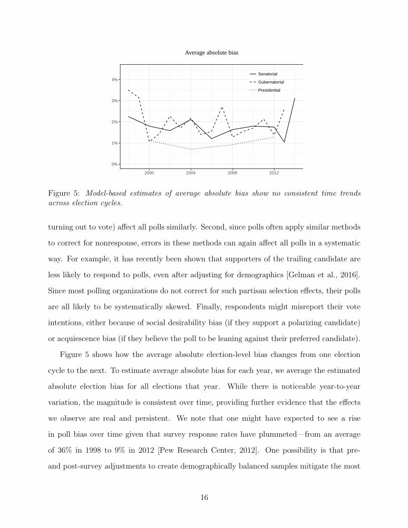
Figure 5: Model-based estimates of average absolute bias show no consistent time trendsacross election cycles.

turning out to vote) affect all polls similarly. Second, since polls often apply similar methods

to correct for nonresponse, errors in these methods can again affect all polls in a systematic

way. For example, it has recently been shown that supporters of the trailing candidate are

less likely to respond to polls, even after adjusting for demographics [Gelman et al., 2016].

Since most polling organizations do not correct for such partisan selection effects, their polls

are all likely to be systematically skewed. Finally, respondents might misreport their vote

intentions, either because of social desirability bias (if they support a polarizing candidate)

or acquiescence bias (if they believe the poll to be leaning against their preferred candidate).

Figure 5 shows how the average absolute election-level bias changes from one election

cycle to the next. To estimate average absolute bias for each year, we average the estimated

absolute election bias for all elections that year. While there is noticeable year-to-year

variation, the magnitude is consistent over time, providing further evidence that the effects

we observe are real and persistent. We note that one might have expected to see a rise

in poll bias over time given that survey response rates have plummeted—from an average

of 36% in 1998 to 9% in 2012 [Pew Research Center, 2012]. One possibility is that pre-

and post-survey adjustments to create demographically balanced samples mitigate the most

16

−8%

−4%

0%

4%

8%

−8% −4% 0% 4% 8%

Senatorial

Gub

erna

toria

l

−8%

−4%

0%

4%

8%

−8% −4% 0% 4% 8%

Senatorial

Pre

side

ntia

l

−8%

−4%

0%

4%

8%

−8% −4% 0% 4% 8%

Presidential

Gub

erna

toria

l

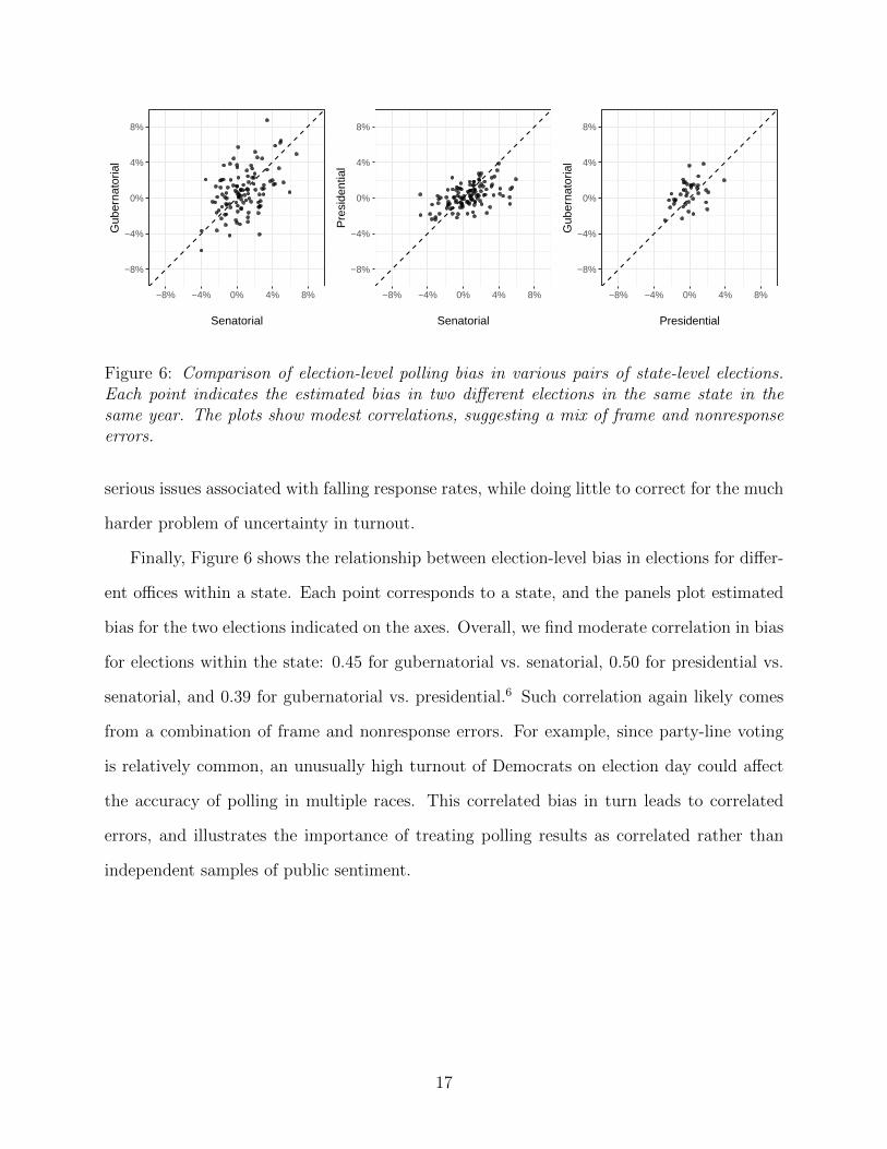
Figure 6: Comparison of election-level polling bias in various pairs of state-level elections.Each point indicates the estimated bias in two different elections in the same state in thesame year. The plots show modest correlations, suggesting a mix of frame and nonresponseerrors.

serious issues associated with falling response rates, while doing little to correct for the much

harder problem of uncertainty in turnout.

Finally, Figure 6 shows the relationship between election-level bias in elections for differ-

ent offices within a state. Each point corresponds to a state, and the panels plot estimated

bias for the two elections indicated on the axes. Overall, we find moderate correlation in bias

for elections within the state: 0.45 for gubernatorial vs. senatorial, 0.50 for presidential vs.

senatorial, and 0.39 for gubernatorial vs. presidential.6 Such correlation again likely comes

from a combination of frame and nonresponse errors. For example, since party-line voting

is relatively common, an unusually high turnout of Democrats on election day could affect

the accuracy of polling in multiple races. This correlated bias in turn leads to correlated

errors, and illustrates the importance of treating polling results as correlated rather than

independent samples of public sentiment.

17

Priors Sen. Gov. Pres.µα, µβ,∼ N(0, 12)σα, σβ ∼ N+(0, 12)στ ∼ N+(0, 0.22)

absolute bias 2.1% 2.3% 1.2%election day absolute bias 2.0% 2.2% 1.2%standard deviation 2.8% 2.7% 2.2%

µα, µβ,∼ N(0, 0.042)σα, σβ ∼ N+(0, 0.042)στ ∼ N+(0, 0.012)

absolute bias 2.0% 2.3% 1.2%election day absolute bias 2.0% 2.2% 1.2%standard deviation 2.8% 2.7% 2.2%

µα, µβ,∼ N(0, 0.042)σα, σβ ∼ Gamma−1(3.6, 0.4)στ ∼ Gamma−1(3.6, 0.1)

absolute bias 1.9% 2.1% 1.1%election day absolute bias 1.8% 2.0% 1.0%standard deviation 3.3% 3.4% 2.9%

Table 2: Posterior estimates for various choices of priors. Our results are nearly identicalregardless of the priors selected.

4.3 Sensitivity analysis

We conclude our analysis by examining the robustness of our results to the choice of

priors in the model. In our primary analysis, we consider a 5 percentage point (equivalent

to 0.2 on the logit scale) standard deviation for the bias and variance hyper-parameters. In

this section, we consider three alternative choices. First, we change the standard deviation

defined for all hyper-parameters to 25 percentage points, corresponding to a prior that is

effectively flat over the feasible parameter region. Second, we change the standard deviation

to one percentage point, corresponding to an informative prior that constrains the bias

and excess variance to be relatively small. Finally, we replace the half-normal prior on the

variance hyper-parameters with an inverse gamma distribution; α and β were chosen so

that the resulting distribution has mean and variance approximately equal to that of the

half normal distribution in the original setting. Table 2 shows the results of this sensitivity

analysis. Our posterior estimates are stable in all cases, regardless of which priors are used.

While the posterior estimates for absolute bias are nearly identical, inverse gamma priors

for variance hyper-parameters result in higher estimated standard deviation for elections.

6To calculate these numbers, we removed an extreme outlier that is not shown in Figure 3, which corre-sponds to polls conducted in Utah in 2004. There are only two polls in the dataset for each race in Utah in2004.

18

5 Discussion

Researchers and practitioners have long known that traditional margins of error under-

state the uncertainty of election polls, but by how much has been hard to determine, in part

because of a lack of data. By compiling and analyzing a large collection of historical election

polls, we find substantial election-level bias and excess variance. We estimate average ab-

solute bias is 2.1 percentage points for senate races, 2.3 percentage points for gubernatorial

races, and 1.2 percentage point for presidential races. At the very least, these findings sug-

gest that care should be taken when using poll results to assess a candidate’s reported lead

in a competitive race. Moreover, in light of the correlated polling errors that we find, close

poll results should give one pause not only for predicting the outcome of a single election,

but also for predicting the collective outcome of related races. To mitigate the recognized

uncertainty in any single poll, it has become increasingly common to turn to aggregated poll

results, whose nominal variance is often temptingly small. While aggregating results is gen-

erally sensible, it is particularly important in this case to remember that shared election-level

poll bias persists unchanged, even when averaging over a large number of surveys.

The 2016 U.S. presidential election offers a timely example of how correlated poll errors

can lead to spurious predictions. Up through the final stretch of the campaign, nearly all

pollsters declared Hillary Clinton the overwhelming favorite to win the election. The New

York Times, for example, placed the probability of a Clinton win at 85% on the day before

the election. Donald Trump ultimately lost the popular vote, but beat forecasts by about 2

percentage points. He ended up carrying nearly all the key swing states, including Florida,

Iowa, Pennsylvania, Michigan, and Wisconsin, resulting in an electoral college win and the

presidency. Because of shared poll bias—both for multiple polls forecasting the same state-

level race, and also for polls in different states—even modest errors significantly impact win

estimates. Such correlated errors might arise from a variety of sources, including frame

errors due to incorrectly estimating the turnout population. For example, a higher-than-

expected turnout among white men, or other Republican-leaning groups, may have skewed

19

poll predictions across the nation.

Our analysis offers a starting point for polling organizations to quantify the uncertainty

in predictions left unmeasured by traditional margins of errors. Instead of simply stating

that these commonly reported metrics miss significant sources of error, which is the status

quo, these organizations could—and we feel should—start quantifying and reporting the gap

between theory and practice. Indeed, empirical election-level bias and variance could be

directly incorporated into reported margins of error. Though it is hard to estimate these

quantities for any particular election, historical averages could be used as proxies.

Large election-level bias does not afflict all estimated quantities equally. For example,

it is common to track movements in sentiment over time, where the precise absolute level

of support is not as important as the change in support. A stakeholder may primarily be

interested in whether a candidate is on an up or downswing rather than his or her exact

standing. In this case, the bias terms—if they are constant over time—cancel out.

Given the considerable influence election polls have on campaign strategy, media narra-

tives, and popular opinion, it is important to not only have accurate estimates of candidate

support, but also accurate accounting of the error in those estimates. Looking forward,

we hope our analysis and methodological approach provide a framework for understanding,

incorporating, and reporting errors in election polls.

20

References

Stephen Ansolabehere and Thomas R. Belin. Poll faulting. Chance, 6, 1993.

Paul P. Biemer. Total survey error: Design, implementation, and evaluation. Public Opinion

Quarterly, 74(5):817–848, 2010. ISSN 0033-362X.

Gallup. Gallup world poll research design. http://media.gallup.com/WorldPoll/PDF/

WPResearchDesign091007bleeds.pdf, 2007. Accessed: 2016-04-07.

Andrew Gelman and Jennifer Hill. Data Analysis Using Regression and Multi-

level/Hierarchical models. Cambridge University Press, 2007.

Andrew Gelman, Sharad Goel, Douglas Rivers, and David Rothschild. The mythical swing

voter. Quarterly Journal of Political Science, 2016.

Andrew Gelman et al. Prior distributions for variance parameters in hierarchical models

(comment on article by browne and draper). Bayesian analysis, 1(3):515–534, 2006.

Robert M. Groves and Lars Lyberg. Total survey error: Past, present, and future. Public

Opinion Quarterly, 74(5):849–879, 2010. ISSN 0033-362X.

Matthew D. Hoffman and Andrew Gelman. The no-U-turn sampler: Adaptively setting

path lengths in Hamiltonian Monte Carlo. Journal of Machine Learning Research, 15

(Apr):1593–1623, 2014.

Sharon Lohr. Sampling: Design and Analysis. Nelson Education, 2009.

Sam G. McFarland. Effects of question order on survey responses. Public Opinion Quarterly,

45(2):208–215, 1981.

Pew Research Center. Assessing the representativeness of public opinion surveys.

http://www.people-press.org/2012/05/15/assessing-the-representativeness-of-public-

opinion-surveys, 2012. Accessed: 2016-04-07.

21

Pew Research Center. Our survey methodology in detail. http://www.people-press.org/

methodology/our-survey-methodology-in-detail, 2016. Accessed: 2016-04-07.

Tom W. Smith. That which we call welfare by any other name would smell sweeter: An

analysis of the impact of question wording on response patterns. Public Opinion Quarterly,

51(1):75–83, 1987.

D. Stephen Voss, Andrew Gelman, and Gary King. Pre-election survey methodology: Details

from nine polling organizations, 1988 and 1992. Public Opinion Quarterly, 59:98–132, 1995.

22