DISCUSSION PAPERS IN ECONOMICS

Working Paper No. 19-01

A Hardware Approach to Value Function Iteration

Alessandro Peri University of Colorado Boulder

June 13, 2019

Department of Economics

University of Colorado Boulder Boulder, Colorado 80309

© June 2019 Alessandro Peri

A Hardware Approach to Value Function IterationI

June 13, 2019Latest Version: Link

Alessandro Peri

University of Colorado Boulder

Abstract

We propose a novel approach for the computation of dynamic stochastic equilibrium models.

We design an FPGA specialized in the computation of a bellman equation via value function

iteration (VFI). Our hardware approach documents significant speed gains vis-a-vis GPU-

based data-parallelization techniques. The speed gains arise from two layers of parallelism,

accessible to hardware developers: instruction-level and pipeline parallelism at the logical

resources level. By and large, the paper highlights significant computational speed gains from

hardware specialization.

JEL Classification: C88.

Key Words: FPGA, Economics, Bellman Equation, Value Function Iteration

People who are really serious about software should make their own hardware - Alan Kay

Steve Jobs, iPhone Keynote, 2007

1. Introduction

How do we get the most out of our scarce resources? We specialize. This paper illustrates

an application of this principle to the field of computational economics.

From the genesis of the Internet of Things to the development of machine learning, the

rise of the Information Age has witnessed an unprecedented increase in the demand for

I Ackowledgement : I am sincerely indebted to Alessandro Nale for his contribution in designing the FPGAsolution proposed in this paper. I wish to thank Jesus Fernandez-Villaverde and Tom Holden for valuableinsights. I also wish to thank Martin Boileau, Terrance Iverson, Richard Mansfield, Miles Kimball, and all theparticipants to the CU Boulder Macro Brownbag (Apr 2018), Bundesbank (Dec 2018) for helpful suggestions.

Email address: alessandro.peri@colorado.edu (Alessandro Peri)URL: https://sites.google.com/site/alessandroperiphd/ (Alessandro Peri)

computational power. In order to cope with this technological challenge, major corporations

- like Google, Intel and Microsoft - have recently stopped relying on commodity general

purpose hardware (i.e. CPUs) and have instead started developing their own chips. In

2017, Google presented its custom accelerator for machine learning applications: the Tensor

Processing Unit (TPU). Using the words of a distinguished hardware engineer at Google:

“This is roughly equivalent to fast-forwarding technology about seven years into the future

(three generations of Moore’s Law)”.1

The main contribution of this paper is to bring this hardware approach to the macroe-

conomists’ table. To this end, we propose a class of chips, whose hardware is explicitly

designed to be fully customizable by the user: the Field-programmable gate array (FPGA).

Following Aldrich et al. [2011], we illustrate the potential of this technology in a standard

RBC model. We design an FPGA specialized in the solution of a bellman equation via

value function iteration (FPGA approach). In doing so, we present a novel parallelization

scheme (the assembly line algorithm) and compare the speed gains vis-a-vis the GPU data-

parallelization scheme proposed in Aldrich et al. [2011] (GPU approach). Our work documents

∼10-fold speed gains in the solution of the bellman equation via value function iteration, on a

state space with 65536 and 4 points in the capital and productivity shock grids, respectively.

The speed gains are a byproduct of hardware specialization. FPGAs are integrated circuits

with (billions of) tiny transistors, organized in configurable logic blocks (CLBs)2. Differently

from CPUs and GPUs, the connections among FPGA’s transistors are not pre-designed by

the manufacturer. On the contrary, hardware developers can fully customize the routing

network between the CLBs3 to accelerate their target application. In this paper, we specialize

the FPGA’s hardware to solve a bellman equation via value function iteration. This approach

1“Google supercharges machine learning tasks with TPU custom chip.”, Jouppi [2016].2 See Appendix A for an overview of the FPGA, CPU and GPU platforms.3 Hardware developers can describe an FPGA image using description languages like VHDL (VHSIC

Hardware description language) or Verilog.

2

grants access to two layers of parallelism, unaccessible to software developers: i) instruction-

level and ii) pipeline parallelism at the logical (CLB) resources level. Intuitively speaking, the

former determines the operations to be performed in parallel at every clock cycle, while the

latter organizes their synchronous execution along an assembly line. Inspired by its analogy

to Ford’s assembly line, we call this parallelization scheme the assembly line parallelism4.

The FPGA approach has proven extremely successful in a variety of sectors and fields5, from

genomics, medicine6, physics7 to banking and finance8. The chip is indeed particularly suited

for practical research purposes. First, conditional on knowing the hardware design principles9,

it is easily programmable10. Second, it saves the infrastructure costs and maintainance of a

cluster. Third, it fits any workstation.

In this context, the launch in 2017 of Unix Instances connected to FPGA chips (EC2

F1 Instances) on the Amazon AWS cloud platform could represent a breakthrough for the

diffusion of FPGA-acceleration, for at least two reasons. First, the cloud service dramatically

reduces the cost of entry to the FPGAs technology, by allowing users to lease instead of buying

the chip. Second, and more far-reaching, it allows developers to upload their FPGA images

4 Our assembly line parallelism draws on Henry Ford’s idea of organizing specalized workers aroundan assembly line, where the output of one worker is the input of another. This technique has been vastlyexploited by hardware engineers to boost CPUs and GPUs’ performance. As CPUs are designed to efficientlyexecute serial operations, they possess extremely efficient instruction pipelines (e.g., the RISC pipelines). AsGPU are designed to efficiently create and manipulate images, they possess extremely efficient graphicalpipelines (e.g. pipelines to speed up rendering operations). In the same spirit, as our FPGA is designed tosolve bellman equations via value function iteration, it possesses a pipeline that efficiently: 1) dissembles thevalue function iteration algorithm in its atomic operations; and 2) organizes them back around an assemblyline.

5 For a comprehensive review, visit the Xilinx webpage https://www.xilinx.com/applications.html.6 In genomics, it contributed to the introduction of high-speed “Next-Gen” DNA sequencing (Margulies

et al. [2005]) that bolstered breakthrough discoveries in medicine - supporting the first deep sequencing of atumor (Thomas et al. [2006]) with associated changes in cancer patients care.

7 Most recently, FPGA chips have been used for the digital signal processing operations that yielded thefirst image of a black hole (Akiyama et al., 2019).

8 See De Schryver [2015]) for a review.9 The entry cost to these principles may be easily circumvented by hiring/coauthoring with researchers

specialized in FPGA’s programming.10 Appendix B describes the similarities between FPGA and software programming.

3

on the cloud, facilitating the sharing of FPGA’s algorithms. For instance, the interested

reader can deploy our FPGA solution, by launching in Amazon AWS the Amazon Machine

Image (AMI): FPGA - Value Function Iteration Accelerator11.

Like the fall in the cost of DNA sequence has fostered breakthrough discoveries in genomics

and medicine, the fall in the entry costs to the FPGA technology provides an important venue

for the research and development of high-speed algorithms in macroeconomics. Fostered by

the recent development of heterogenous agents-model featuring nominal rigidities (Bayer

et al. [2019]) and a growing attention to the distributional effect of government policies, the

FPGA approach could find a promising area of application in the complex (and sometimes

unfeasible) estimation of heterogenous agents model. This paper provides a first step in this

direction, discussing the acceleration of one of the most expensive computational bottlenecks

involved in this process: the solution of a bellman equation.

By and large, these considerations suggest the presence of significant gains from hardware

specialization, so far unexplored by the macroeconomic literature.

2. Contribution

The optimization problem of agents with rational preferences rests at the heart of virtually

every macroeconomic model. In this context, the bellman equation (Bellman, 1957) is a

powerful tool that simplifies complex infinite-horizon maximization problems into two-period

problems of the form

V (x, z) = T (V ) = maxx′∈Γ(x,z)

F (x, z, x′) + β ·∫z′∈Z

V (x′, z′)Q(dz′, z) (1)

where agents observe the state (x, z) ∈ X × Z and choose a control x′ ∈ Γ(x, z) to maximize

current F (x, z, x′) and expected discounted payoffs β ·∫Z

V (x′, z′)Q(dz′, z).

11 AWS Link: https://aws.amazon.com/marketplace/pp/B07PLWCNCV

4

Yet, solving a Bellman Equation is computationally challenging. Under suitable assump-

tions - described in the Banach Contraction Mapping Theorem (see, Stokey et al. [1989]) - it

is possible to approach arbitrarily close the limit function V , starting from any guess V0(·)

and iterating over the operator T nV0(·),

ρ(T nV0, V ) ≤ 1

1− βρ(T nV0, T

n+1V0) < ε

This approach may take many steps. In addition, the estimation of the structural parameters

may require solving the bellman equation several times, often in the order of millions.

The literature has coped with this computational challenge by proposing solutions that

(for the sake of exposition) fall into two categories: a software and a hardware approach.

The software approach focuses on developing efficient algorithms to solve the bellman

equation. Generally speaking, these algorithms exploit theoretical properties of the value

function to improve speed and/or accuracy12.

The hardware approach complements the software approach, by exploiting parellel com-

puting techniques in order to distribute the computational burden across several processing

units13. The standard in high performance computing is to use message passing systems

(like openMP and open MPI) to parallelize the peak-finding algorithm by distributing the

evaluation of the objective function at different grid points (x, z) ∈ X × Z across several

cores (data parellelism). As of today, this approach requires the set-up and maintainance of

complex infrastructure, like clusters, massively parellel processing (MPPs) and grids. Most

recently, Aldrich et al. [2011] illustrate the potential of a much lighter hardware platform that

would fit any workstation: the graphics processing units (GPU). GPUs are particularly apt

to exploit the type of data level parellelism involved in the computation of bellman equations

12 See Aruoba et al. [2006] for a review and discussion of these methods in the context of an RBC; 2)refined maximization procedure (e.g., Fella [2014], Gordon and Qiu [2015]).

13 See Fernandez-Villaverde and Valencia [2018] for a practical guide to parallel computing in economics.

5

via value function iteration, owing to their rich endowments of processing units (ranging from

100 to 5000 cores). In their seminal paper, Aldrich et al. [2011] document speed gains akin to

parallelizations on small scale super-computers.

This paper builds a bridge between these two approaches: we propose a chip (the FPGA)

that allows the implementation of (software) algorithms at the hardware level.

The rest of the paper is organized as follows. Section 3 lays out the model. Section 4

discusses the computational algorithm. Section 5 introduces the assembly line parallelism.

Section 6 presents the results and examines the origins of the speed gains: the assembly line

parallelism. Section 7 discusses applications and extensions. Section 8 concludes.

3. The Model

In the spirit of Aldrich et al. [2011], we illustrate the FPGA approach in the context of a real

business cycle model. The representative household chooses consumption c and capital k′ to

solve the bellman equation

V (k, z) = maxc,k′

c1−η

1− η+ β ·

∫z′V (k′, z′)Q(z′, z)dz′ (2)

s.t. c+ k′ = zkα + (1− δ)k

where the log-productivity z follows an AR(1)

ln zt+1 = ρ ln zt + εt+1, εt+1 ∼ N(0, σ2

)(3)

The model has 6 parameters. For the sake of comparison, we calibrate them as in Aldrich et al.

[2011] to match features of the U.S. quarterly data: risk aversion η = 2, subjective discount

factor β = 0.984, return to scale parameter α = 0.35, depreciation rate δ = 0.01, persistence

of the log-productivity shock ρ = 0.95, volatility of the innovation on the log-productivity

6

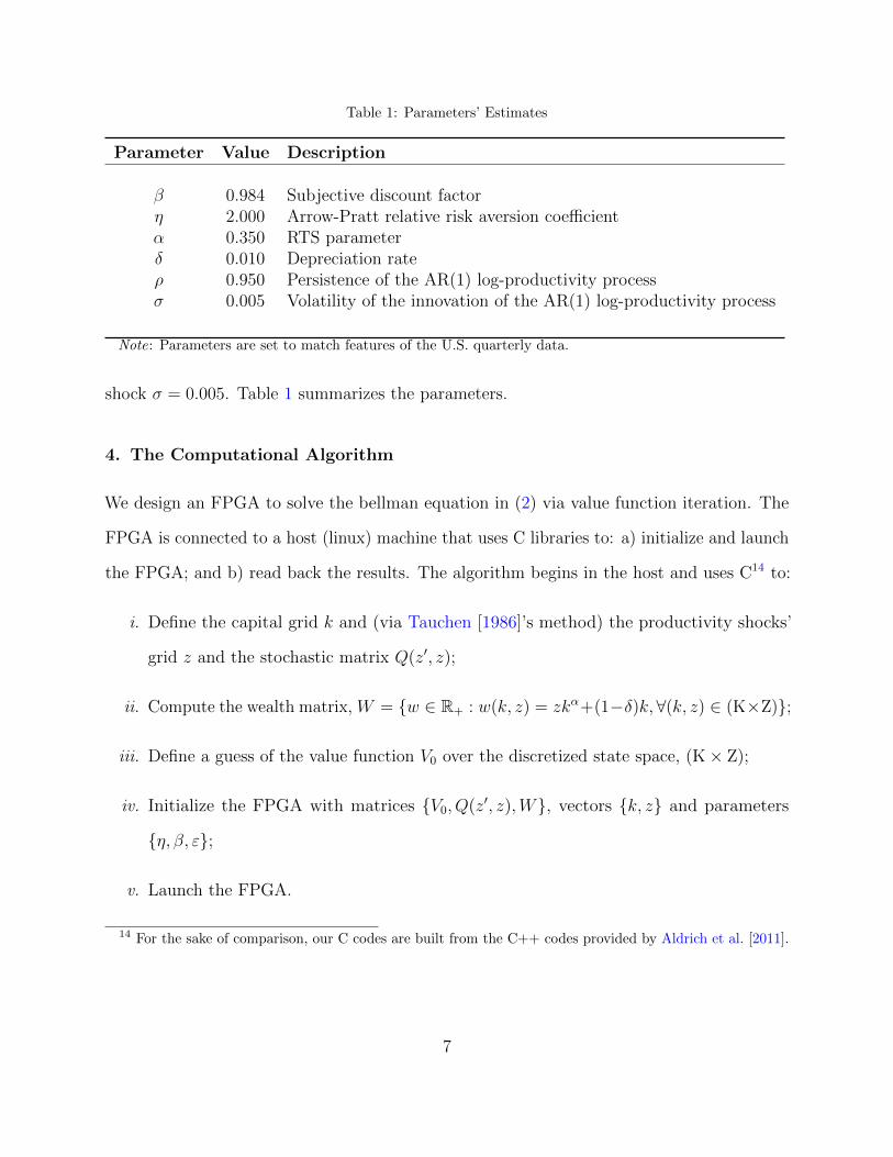
Table 1: Parameters’ Estimates

Parameter Value Description

β 0.984 Subjective discount factorη 2.000 Arrow-Pratt relative risk aversion coefficientα 0.350 RTS parameterδ 0.010 Depreciation rateρ 0.950 Persistence of the AR(1) log-productivity processσ 0.005 Volatility of the innovation of the AR(1) log-productivity process

Note: Parameters are set to match features of the U.S. quarterly data.

shock σ = 0.005. Table 1 summarizes the parameters.

4. The Computational Algorithm

We design an FPGA to solve the bellman equation in (2) via value function iteration. The

FPGA is connected to a host (linux) machine that uses C libraries to: a) initialize and launch

the FPGA; and b) read back the results. The algorithm begins in the host and uses C14 to:

i. Define the capital grid k and (via Tauchen [1986]’s method) the productivity shocks’

grid z and the stochastic matrix Q(z′, z);

ii. Compute the wealth matrix, W = {w ∈ R+ : w(k, z) = zkα+(1−δ)k,∀(k, z) ∈ (K×Z)};

iii. Define a guess of the value function V0 over the discretized state space, (K× Z);

iv. Initialize the FPGA with matrices {V0, Q(z′, z),W}, vectors {k, z} and parameters

{η, β, ε};

v. Launch the FPGA.

14 For the sake of comparison, our C codes are built from the C++ codes provided by Aldrich et al. [2011].

7

Second, the FPGA solves the value function iteration step i

V i(k, z) = maxk′∈K

F (k, z, k′) + β ·∑z′

V i−1(k′, z′)Q(z′, z)dz′

up to convergence of the value function ||V i − V i−1|| < ε. In particular,

1. Given V0, the FPGA uses the binary search algorithm discussed in Section 4.0.1

(and detailed in Appendix C.2.1) to solve the value function iteration step for any

(k, z) ∈ K× Z and get a new guess of the value function V1;

2. Let || · || = sup(k,z)∈K×Z

| · | denote the sup-norm. If the update satisfies the convergence

criterion ||V1 − V0|| < ε, convergence is reached and the algorithm exits the loop.

Otherwise, the FPGA sets V0 = V1, and iterates over 1-2 until convergence.

Once the convergence is reached, the host reads the value function V ∗1 and policy function

G∗ back.

4.0.1. Binary Search Algorithm

The maximization is performed using the recursive binary-search algorithm developed in

Appendix C.215. The algorithm reaches a solution in 15 stages. At each binary stage

n ∈ {1, 2, . . . , 14, 15} the algorithm:

1. Evaluates the objective function at three nth-stage indexes {i(n, j)}j∈{1,2,3}, with the

exception of the final stage, where the algorithm evaluates the objective function at 4

indexes {i(n, j)}j∈{1,2,3,4}.

2. Determines the nth-stage indexes {i(n, j)}j∈{1,2,3} using a recursive selection rule16 that

depends on the (n − 1)th-stage maximizer j∗(n − 1) and a sufficient statistic of the

15 The interested reader can refer to the appendix for all the details.16 To the best of our knowledge we are the first to propose this selection rule.

8

history of previous binary-stages’ maximizers h∗(n− 1).

5. The Assembly Line Parallelism

Each value function iteration step i

V i(k, z) = maxk′∈K︸︷︷︸

Peak-Finding

F (k, z, k′) + β ·∑z′

V i−1(k′, z′)Q(z′, z)dz′︸ ︷︷ ︸Objective Function h(k,z,k′)

involves two distinct operations: 1) the evaluation of the objective function, h(k, z, k′); and

2) the peak-finding algorithm.

Figure 1: The Assembly Line Parallelism

1

0

j*(n-1)

Stage 2Stages 3...14

Stage 15

+

V(k,z)

(z,w(k,z))Stage Delay Stage Delay Stages Delay

h*(n-1)

(z,w(k,z))

j*(n)

h*(n)

j*(n-1)

h*(n-1)

(z,w(k,z))

h(k,z,k'(i(n,j*)))

j*(n)

h*(n)

j*(n-1)

h*(n-1)

(z,w(k,z))

j*(n)

h*(n)i*(k,z)

Stage 1

h(k,z,k'(i(n,j*)))h(k,z,k'(i(n,j*)))

Note: The figure illustrates the organization of the 15 binary stages along the assembly line. Given thestate (z, k), the previous stage maximizer j∗(n− 1) and a sufficient statistic of the history of previousbinary-stages’ maximizers h∗(n − 1), each binary-stage updates j∗(n) and h∗(n). After 15 stages, theassembly line returns the value function V (k, z) and maximiser i∗(k, z).

The instruction-level and pipeline parallelism operate on both these dimensions. On one

side, the instruction-level parallelism determines the operations to be performed in parallel

at every clock cycle. The appendix details how the algorithm parallelizes the instructions

involved in the computation of the objective function (Appendix C.1) and in each binary stage

(Appendix C.3). On the other side, the pipeline parallelism exploits the recursive structure of

9

the binary search algorithm to organize the synchronous execution of these operations along

an assembly line, as illustrated in Figure 1 (and detailed in Figure C.7).

6. Implementation and Results

This section compares and discusses the time required to solve the bellman equation via value

function iteration in the GPU and FPGA chips, using the binary search algorithm discussed

in Section 4.0.1 (and detailed in Appendix C.2.1).

Table 2: Solution Time Comparison

FPGA GPU

TimeInitialization 0.25 0.01Solution 1.42 13.69Reading 0.75 0.01Total 2.42 13.71

Platforms’ Technical SpecificationASICs 16 nm Xilinx UltraScale Plus NVIDIA Tesla K80Max Clock (MHz) 250 875Cores - 4992

Note: Time (in seconds) to find the solution to the Bellman equation via value function iteration in theFPGA (Col 1) and in the GPU (Col 2) using the binary search algorithm discussed in Section 4.0.1. Thetime is categorized in: allocation of the device (row 1), solution (row 2), transfer of the results back to thehost (row 3) and total (row 4). The results are obtained as averages of 1000 models calibrated as in Table1. The grids on capital has 65536 points. We set ε = 1e-10, where ε is the tolerance of the convergencecriterion ||V1 − V0|| < ε. We set the clock of the FPGA at 250 MHz. Platforms : a) The FPGA results areobtained using a 16 nm Xilinx UltraScale Plus mounted on a node with Intel(R) Xeon(R) CPU E5-2686v4 2.30GHz, 8 CPUs/node. b) The GPU results are obtained using an NVIDIA Tesla K80 with 4992cores mounted on a node with Intel Xeon CPU E5-2680 v3 2.50GHz, 2 CPUs/node.

In the FPGA we implement the assembly line parallelism discussed in Section 5 (and

detailed in Appendix C.3). Conversely, in the GPU we implement the data-parallelization

scheme proposed in Aldrich et al. [2011], since GPUs are: i) best suited for data-parallelism17

17 Due to the lack of high bandwidth access to cached data, GPUs perform at their best in data-parallelprocessing with little reuse of input data. Since the assembly line parallelism makes extensive reuse of cacheddata, it is outperformed in the GPU by the data-parallelism proposed by Aldrich et al. [2011].

10

and ii) do not provide the FPGA’s hardware flexibility necessary for syncronizing the

parallelism at the logical resources (CLB) level18.

Table 2 reports the results. The FPGA results are obtained using a 16 nm Xilinx

UltraScale Plus mounted on a node with Intel(R) Xeon(R) CPU E5-2686 v4 2.30GHz, 8

CPUs/node. The GPU results are obtained using an NVIDIA Tesla K80 with 4992 cores

mounted on a node with Intel Xeon CPU E5-2680 v3 2.50GHz, 2 CPUs/node.

Our simulations record significant speed gains: the FPGA is 9.64 times faster than the

GPU (13.69 vs 1.42) in solving the bellman equation (C.2) via VFI using the binary search

algorithm. For completeness, we also report the time required to initialize and read back

the results from the chips. The GPU outperforms the FPGA in this context. If we factor

in these components the FPGA is approximately 6 times faster. Importantly, the network

interconnection between the host and guest machines (FPGA and GPU) are similar, so

future developments in this dimension are likely to drastically reduce this difference19. While

we acknowledge the presence of important margins of improvement in this dimension, we

also take the occasion to stress that the final goal of this paper is to introduce the FPGA

technology and to illustrate its potential for accelerating the solution’s time of a bellman

equation.

The speed gains arise from the possibility of synchronizing the parallelism at the logical

resources (CLB) level. As a result, although GPU’s cores are up to three times faster than

our FPGA’s clock, the gains from hardware specialization more than offset the lower clock

speed. The next session explores the determinants of the speed gains, by investigating the

assembly line parallelism workflow.

18 Although GPUs allow to program the pipeline parallelism at the binary stage level, they do not allow soat the CLBs level. The GPU’s compiler takes care of this level of detail.

19 The difference that we observe arises from a low performing algorithm in the communication with theFPGA. In particular, the C code copies and reads information from and to the FPGA element by elementrather than in blocks.

11

6.1. The Assembly Line Parallelism Workflow

This section exploits the analogy between the pipeline algorithm and Ford’s assembly line to

illustrate the assembly line parallelism workflow.

Figure 2: The assembly line parallelism workflow

1

0

j*(n-1)

(z,w(k,z))

h*(n-1)

(z,w(k,z))

j*(n)

h*(n)

Stage 1

h(k,z,k'(i(n,j*)))

Worker 60

1 Tck

Worker 59Worker 58Worker 3Worker 2Worker 1

z1,k1

2 Tck z1,k2 z1,k1

3 Tck z1,k2 z1,k1z1,k3

58 Tck z1,k57 z1,k56z1,k58

59 Tck z1,k58 z1,k57z1,k59

60 Tck z1,k59 z1,k58z1,k60 z1,k2 z1,k1z1,k3

z1,k2 z1,k1

z1,k1

Stage 2Stages 3...14

Stage 15

+

V(k,z)j*(n-1)

h*(n-1)

(z,w(k,z))

h(k,z,k'(i(n,j*)))

j*(n)

h*(n)

j*(n-1)

h*(n-1)

(z,w(k,z))

j*(n)

h*(n)i*(k,z)

h(k,z,k'(i(n,j*)))

Worker 2Worker 1

z1,k2 z1,k1z1,k3

z1,k2 z1,k1

z1,k4

z1,k3z1,k4z1,k5

61 Tck z1,k60 z1,k59z1,k61

62 Tck z1,k61 z1,k60z1,k62

Worker 60Worker 59

z1,k2 z1,k1

Stage 1,..15 Loaded

900 Tck V(k1,z1)

z1,k3 z1,k2 V(k2,z1)901 Tck

902 Tck z1,k3 V(k3,z1)

1 Tck

1 Tck

z1,k4

z1,k899 z1,k898z1,k900

z1,k900 z1,k899z1,k901

z1,k901 z1,k900z1,k902

Note: This figure illustrates the assembly line workflow associated to each iteration step V i = T iV 0. Thehorizontal dimension denotes the allocation of FPGA resources, while the vertical dimension denotes theevolution of time.

The pipeline algorithm orders the binary stages around the assembly line. Each binary

stage is organized like a team of workers. Each worker - defined as a set of logical units like

DSP and CLBs - is assigned a position (and task) in front of the assembly line treadmill -

12

defined as the set of registers connected to the master signal.

Figure 2 illustrates the time evolution (vertical dimension) of the assembly line workflow

(horizontal dimension) inside the FPGA. In each clock cycle, a worker reads information

from the assembly line treadmill, performs a set of instructions, and returns the result on the

treadmill. For example, in the first clock cycle 1Tck (first row), worker 1 reads the first state

variables (z1, k1) (white circle), performs her task, and returns the result on the treadmill.

In the next clock cycle 2Tck (second row), worker 2 (idle until now) reads the results of

worker 1 on (z1, k1) (white circle), performs her task, and returns the result on the treadmill.

Meanwhile, worker 1 has already started working on the second input (z1, k2) (blue circle).

So, after two clock cycles the assembly line has two operations performed in parallel. As time

unfolds, the assembly line is gradually loaded with new state variables. After 60 clock cycles,

60 workers are operating in parallel, the first binary stage is completed and the second binary

stage is about to start. After 900 clock cycles, the 15 binary stages are fully loaded and the

assembly line returns the first value function V1(k1, z1) and maximizer i∗(k1, z1). From this

moment on, the FPGA starts producing at full potential: at every clock cycle it yields a new

V1(ki, zi).

What determines the pace of the assembly line treadmill? The clock is the single master

signal that determines the speed at which all operations in the circuitry act simultaneously.

In principle, the faster the clock the faster results are produced. Yet, the clock speed cannot

be set arbitrarily high. If the clock is too fast, the FPGA workers are not able to perform

their operations at the required pace and return wrong results.

In order to increase the speed, the hardware developer can exploit the trade-off between

logical resources and speed. The idea behind this optimization strategy is very simple: having

more workers doing less. Reducing the instructions per worker, at the cost of a longer

treadmill (registers) and more workers (logical resources) allows to increase the clock speed.

Yet, this strategy faces two constraints. First, a longer treadmill with more workers consume

13

more logical resources and registers, up to the point of congestion of the FPGA. Second, the

fact that instructions are not infinitely divisible limits how many workers can be added.

In our implementation, we exploit this trade-off and push the clock of the FPGA up to

250 MHz (250 millions of jobs per second). So once full, our assembly line returns V1(ki, zi)

every 4.00ns (1/250 MHz).

At this point, rationalizing the speed gains is an accounting exercise. Given that conver-

gence is reached after 1352 iterations (when the tolerance is ε =1e-10), the time required

to estimate the value function (net of negligible overhead time costs) on the state space of

(Nk, Nz) = (65536, 4) can be computed using the following decomposition

Time = 1352︸︷︷︸No Iterations

· 65536︸ ︷︷ ︸Nk

· 4︸︷︷︸Nz

· 1

250 · e6︸ ︷︷ ︸Clock

= 1.42 sec (4)

7. Case Study and Policy Implications

The FPGA approach has proven extremely successful in a variety of sectors and fields, from

genomics, medicine to physics and finance. This section discusses an application in the

context of risk management during the financial crises.

Notably, while the theoretical limits in the forecasting ability of risk models have received

general attention by the financial literature20, the computational limits in the estimation of

these models have been vastly neglected. Amidst the financial turmoil, the estimation of the

risk parameters of JP Morgan complex derivative portfolios required more than 10 hours in

a cluster of thousands of cores (Feldman [2011]). This delay was long enough to make the

information content of the estimates obsolete21, exacerbating the well-documented inability

20 Such as Danıelsson [2002], Danıelsson [2008], fostering research on risk measures (Frittelli et al., 2014)and changes in the regulations of banking (Basel III) and insurance (Solvency II) industries.

21Using the words of his leading manager Stephen Weston, “It was a bit like driving your car on the freewayat 90 miles per hour by looking in the rear view mirror. It could be fun, but there’s a high probability itcould be a destructive activity.”

14

of risk models to account for systemic risk. In 2011, JP Morgan directly tackled the problem.

After a first attempt to accelerate their estimation via GPUs (with a 15-fold speed-up), they

hired a specialized company to take advantage of FPGA chips. The new platform reduced

the execution time by a factor of 130, from 10 hours to 4 minutes. More far-reaching, the

gains of relaxing the computational feasibility constraint went beyond the faster execution

of the estimation. Traders were able to change the parameterization of the model to assess

different scenarios and better inform their investment decisions.

This case study shows important micro-prudential policy implications of FPGA acceler-

ation. Similarly, the growing attention to the distributional effect of government policies -

fostered by the recent development of heterogenous agents-model featuring nominal rigidities

(Bayer et al. [2019]) - suggests that the FPGA approach could find a promising area of

application in the complex (and sometimes unfeasible) estimation of heterogenous agents

models22.

8. Conclusions and Extensions

In the last decades, the use of highly-specialized chips (like, FPGAs and ASICs) has be-

come pervasive across several sectors and fields. From bitcoin mining to machine learning

accelerators, there has been a growing acknowledgment of the gains arising from hardware

specialization. The main contribution of this paper is to bring this “hardware” approach to

the macroeconomists’ table.

To this end, we design a Field-programmable gate array (FPGA) specialized in the

solution of bellman equations via value function iteration. Our hardware approach proposes a

22 Although, these models provide a powerful tool to quantitatively assess the effect of government policieson firms and households’ distributions, the richness of predictions is hindered by their computationallyexpensive and time consuming estimations. The global search over the parameters’ space may require solvingthe bellman equation several times (even in the order of millions), restricting the richness of heterogeneitythat can be studied. In addition, as the number of parameters to be estimated rise, the estimation slips intothe curse of dimensionality problem and may become unfeasible.

15

novel parallelization scheme and documents significant speed gains vis-a-vis GPU-based data-

parallelization techniques. The speed gains are a byproduct of the hardware specialization.

The hardware flexibility grants access to two levels of parallelism, which are unavailable

to software developers: i) the instruction-level and ii) pipeline parallelism at the logical

resources level. We label this parallelization scheme as the assembly line parallelism.

This paper highlights the presence of important gains from FPGA acceleration in the

context of heterogenous agents model, which we plan to explore in our future research.

Importantly, the plethora of computational issues in economics which could benefit from

FPGA-acceleration goes beyond the solution of bellman equations. Since FPGAs are best

suited to handle large scale computational problems whose solutions are computationally

intensive and exploit a recursive algorithm, machine learning, montecarlo simulations, and

maximum likelihood estimation seem promising areas of application.

To conclude, we would like to discuss a venue that could significantly reduce the cost

of access to the FPGA technology: the use of FPGA compiler specialized in translating

C/Matlab codes into customized digital circuits23. Although the use of FPGA compilers is

not yet the standard in the FPGA designers world, recent years have shown signs of early

adoption. Drawing from the successful experience of C compilers in replacing the direct

assembler programming of CPU, major developments in FPGA compilers could drammatically

reduce the cost of access to the FPGA acceleration in the years to come.

Far from claiming the existence of “one chip to rule them all”, our work highlights

the presence of important gains from hardware specialization, so far unexplored by the

macroeconomic literature.

23Among others the Fpga C compiler and the Matlab HDL Coder.

16

References

Akiyama, K., A. Alberdi, W. Alef, K. Asada, R. Azulay, A.-K. Baczko, D. Ball, M. Balokovic,J. Barrett, D. Bintley, L. Blackburn, W. Boland, K. L. Bouman, G. C. Bower, M. Bremer,C. D. Brinkerink, R. Brissenden, S. Britzen, A. E. Broderick, D. Broguiere, T. Bronzwaer, D.-Y. Byun, J. E. Carlstrom, A. Chael, C.-k. Chan, S. Chatterjee, K. Chatterjee, M.-T. Chen,Y. Chen, I. Cho, P. Christian, J. E. Conway, J. M. Cordes, G. B. Crew, Y. Cui, J. Davelaar,M. De Laurentis, R. Deane, J. Dempsey, G. Desvignes, J. Dexter, S. S. Doeleman, R. P.Eatough, H. Falcke, V. L. Fish, E. Fomalont, R. Fraga-Encinas, P. Friberg, C. M. Fromm,J. L. Gomez, P. Galison, C. F. Gammie, R. Garcıa, O. Gentaz, B. Georgiev, C. Goddi,R. Gold, M. Gu, M. Gurwell, K. Hada, M. H. Hecht, R. Hesper, L. C. Ho, P. Ho, M. Honma,C.-W. L. Huang, L. Huang, D. H. Hughes, S. Ikeda, M. Inoue, S. Issaoun, D. J. James, B. T.Jannuzi, M. Janssen, B. Jeter, W. Jiang, M. D. Johnson, S. Jorstad, T. Jung, M. Karami,R. Karuppusamy, T. Kawashima, G. K. Keating, M. Kettenis, J.-Y. Kim, J. Kim, J. Kim,M. Kino, J. Y. Koay, P. M. Koch, S. Koyama, M. Kramer, C. Kramer, T. P. Krichbaum, C.-Y.Kuo, T. R. Lauer, S.-S. Lee, Y.-R. Li, Z. Li, M. Lindqvist, K. Liu, E. Liuzzo, W.-P. Lo, A. P.Lobanov, L. Loinard, C. Lonsdale, R.-S. Lu, N. R. MacDonald, J. Mao, S. Markoff, D. P.Marrone, A. P. Marscher, I. Martı-Vidal, S. Matsushita, L. D. Matthews, L. Medeiros, K. M.Menten, Y. Mizuno, I. Mizuno, J. M. Moran, K. Moriyama, M. Moscibrodzka, C. Muller,H. Nagai, N. M. Nagar, M. Nakamura, R. Narayan, G. Narayanan, I. Natarajan, R. Neri,C. Ni, A. Noutsos, H. Okino, H. Olivares, G. N. Ortiz-Leon, T. Oyama, F. Ozel, D. C. M.Palumbo, N. Patel, U.-L. Pen, D. W. Pesce, V. Pietu, R. Plambeck, A. PopStefanija,O. Porth, B. Prather, J. A. Preciado-Lopez, D. Psaltis, H.-Y. Pu, V. Ramakrishnan, R. Rao,M. G. Rawlings, A. W. Raymond, L. Rezzolla, B. Ripperda, F. Roelofs, A. Rogers, E. Ros,M. Rose, A. Roshanineshat, H. Rottmann, A. L. Roy, C. Ruszczyk, B. R. Ryan, K. L. J. Rygl,S. Sanchez, D. Sanchez-Arguelles, M. Sasada, T. Savolainen, F. P. Schloerb, K.-F. Schuster,L. Shao, Z. Shen, D. Small, B. W. Sohn, J. SooHoo, F. Tazaki, P. Tiede, R. P. J. Tilanus,M. Titus, K. Toma, P. Torne, T. Trent, S. Trippe, S. Tsuda, I. van Bemmel, H. J. vanLangevelde, D. R. van Rossum, J. Wagner, J. Wardle, J. Weintroub, N. Wex, R. Wharton,M. Wielgus, G. N. Wong, Q. Wu, A. Young, K. Young, Z. Younsi, F. Yuan, Y.-F. Yuan,J. A. Zensus, G. Zhao, S.-S. Zhao, Z. Zhu, J.-C. Algaba, A. Allardi, R. Amestica, U. Bach,C. Beaudoin, B. A. Benson, R. Berthold, J. M. Blanchard, R. Blundell, S. Bustamente,R. Cappallo, E. Castillo-Domınguez, C.-C. Chang, S.-H. Chang, S.-C. Chang, C.-C. Chen,R. Chilson, T. C. Chuter, R. C. Rosado, I. M. Coulson, T. M. Crawford, J. Crowley,J. David, M. Derome, M. Dexter, S. Dornbusch, K. A. Dudevoir, S. A. Dzib, C. Eckert,N. R. Erickson, W. B. Everett, A. Faber, J. R. Farah, V. Fath, T. W. Folkers, D. C.Forbes, R. Freund, A. I. Gomez-Ruiz, D. M. Gale, F. Gao, G. Geertsema, D. A. Graham,C. H. Greer, R. Grosslein, F. Gueth, N. W. Halverson, C.-C. Han, K.-C. Han, J. Hao,Y. Hasegawa, J. W. Henning, A. Hernandez-Gomez, R. Herrero-Illana, S. Heyminck,A. Hirota, J. Hoge, Y.-D. Huang, C. M. V. Impellizzeri, H. Jiang, A. Kamble, R. Keisler,K. Kimura, Y. Kono, D. Kubo, J. Kuroda, R. Lacasse, R. A. Laing, E. M. Leitch, C.-T. Li,L. C.-C. Lin, C.-T. Liu, K.-Y. Liu, L.-M. Lu, R. G. Marson, P. L. Martin-Cocher, K. D.Massingill, C. Matulonis, M. P. McColl, S. R. McWhirter, H. Messias, Z. Meyer-Zhao,

17

D. Michalik, A. Montana, W. Montgomerie, M. Mora-Klein, D. Muders, A. Nadolski,S. Navarro, C. H. Nguyen, H. Nishioka, T. Norton, G. Nystrom, H. Ogawa, P. Oshiro,T. Oyama, S. Padin, H. Parsons, S. N. Paine, J. Penalver, N. M. Phillips, M. Poirier,N. Pradel, R. A. Primiani, P. A. Raffin, A. S. Rahlin, G. Reiland, C. Risacher, I. Ruiz,A. F. Saez-Madaın, R. Sassella, P. Schellart, P. Shaw, K. M. Silva, H. Shiokawa, D. R.Smith, W. Snow, K. Souccar, D. Sousa, T. K. Sridharan, R. Srinivasan, W. Stahm, A. A.Stark, K. Story, S. T. Timmer, L. Vertatschitsch, C. Walther, T.-S. Wei, N. Whitehorn,A. R. Whitney, D. P. Woody, J. G. A. Wouterloot, M. Wright, P. Yamaguchi, C.-Y. Yu,M. Zeballos, and L. Ziurys (2019). First M87 Event Horizon Telescope Results. II. Arrayand Instrumentation. The Astrophysical Journal 875 (1), L2.

Aldrich, E. M., J. Fernandez-Villaverde, A. Ronald Gallant, and J. F. Rubio-Ramırez (2011).Tapping the supercomputer under your desk: Solving dynamic equilibrium models withgraphics processors. Journal of Economic Dynamics and Control 35 (3), 386–393.

Aruoba, S. B., J. Fernandez-Villaverde, and J. F. Rubio-Ramırez (2006). Comparing solu-tion methods for dynamic equilibrium economies. Journal of Economic Dynamics andControl 30 (12), 2477–2508.

Auclert, A., R. Matthew, and L. Straub (2019). Micro Jumps, Macro Humps: MonetaryPolicy and Business Cycles in an Estimated HANK Model. Unpublished working paper .

Bayer, C., R. Luetticke, L. Pham-Dao, and V. Tjaden (2019). Precautionary Savings,Illiquid Assets, and the Aggregate Consequences of Shocks to Household Income Risk.Econometrica 87 (1), 255–290.

Bellman, R. E. (1957). Dynamic Programming. Princeton University Press.

Bhandari, A., D. Evans, M. Golosov, and T. J. Sargent (2017). Fiscal policy and debtmanagement with incomplete markets. Quarterly Journal of Economics 132 (2), 617–663.

Carroll, C. D. (2006). The method of endogenous gridpoints for solving dynamic stochasticoptimization problems. Economics Letters 91 (3), 312–320.

Danıelsson, J. (2002). The emperor has no clothes: Limits to risk modelling. Journal ofBanking and Finance 26 (7), 1273–1296.

Danıelsson, J. (2008). Blame the models. Journal of Financial Stability 4 (4), 321–328.

De Schryver, C. (2015). FPGA Based Accelerators for Financial Applications.

Farooq, U., Z. Marrakchi, and H. Mehrez (2012). Tree-based heterogeneous FPGA archi-tectures: Application specific exploration and optimization. In Springer, New York, NY,Volume 9781461435, pp. 1–186.

Feldman, M. (2011). JP Morgan Buys Into FPGA Supercomputing. HPCwire,https://www.hpcwire.com/2011/07/13/jp morgan buys into fpga supercomputing/ .

18

Fella, G. (2014). A generalized endogenous grid method for non-concave problems. Reviewof Economic Dynamics 17 (2), 329–344.

Fernandez-Villaverde, J. and D. Z. Valencia (2018). A Practical Guide to Parallelization inEconomics. NBER Working Paper No 24561 , 1–65.

Frittelli, M., M. Maggis, and I. Peri (2014). Risk measures on P(R) and value at risk withprobability/loss function. Mathematical Finance 24 (3), 442–463.

Gordon, G. and S. Qiu (2015). A Divide and Conquer Algorithm for Exploiting PolicyFunction Monotonicity. SSRN Electronic Journal .

Jouppi, N. (2016). Google supercharges machine learning tasks with TPU custom chip. Offi-cial Google Blog, https://cloud.google.com/blog/products/gcp/google-supercharges-machine-learning-tasks-with-custom-chip.

Margulies, M., M. Egholm, W. E. Altman, S. Attiya, J. S. Bader, L. A. Bemben, J. Berka,M. S. Braverman, Y. J. Chen, Z. Chen, S. B. Dewell, L. Du, J. M. Fierro, X. V. Gomes,B. C. Godwin, W. He, S. Helgesen, C. H. Ho, G. P. Irzyk, S. C. Jando, M. L. Alenquer,T. P. Jarvie, K. B. Jirage, J. B. Kim, J. R. Knight, J. R. Lanza, J. H. Leamon, S. M.Lefkowitz, M. Lei, J. Li, K. L. Lohman, H. Lu, V. B. Makhijani, K. E. McDade, M. P.McKenna, E. W. Myers, E. Nickerson, J. R. Nobile, R. Plant, B. P. Puc, M. T. Ronan,G. T. Roth, G. J. Sarkis, J. F. Simons, J. W. Simpson, M. Srinivasan, K. R. Tartaro,A. Tomasz, K. A. Vogt, G. A. Volkmer, S. H. Wang, Y. Wang, M. P. Weiner, P. Yu, R. F.Begley, and J. M. Rothberg (2005). Genome sequencing in microfabricated high-densitypicolitre reactors. Nature 437 (7057), 376–380.

Saxena, A. (2014). Oscars host’s selfie tweet crashes Twitter. Website:https://www.gadgetsnow.com/social/Oscars-hosts-sel .

Stokey, N. L., R. E. Lucas, and E. C. Prescott (1989). Recursive Methods in EconomicDynamics. Harvard University Press.

Tauchen, G. (1986). Finite state markov-chain approximations to univariate and vectorautoregressions. Economics Letters 20 (2), 177–181.

Thomas, R. K., E. Nickerson, J. F. Simons, P. A. Janne, T. Tengs, Y. Yuza, L. A. Garraway,T. LaFramboise, J. C. Lee, K. Shah, K. O’Neill, H. Sasaki, N. Lindeman, K. K. Wong,A. M. Borras, E. J. Gutmann, K. H. Dragnev, R. DeBiasi, T. H. Chen, K. A. Glatt,H. Greulich, B. Desany, C. K. Lubeski, W. Brockman, P. Alvarez, S. K. Hutchison, J. H.Leamon, M. T. Ronan, G. S. Turenchalk, M. Egholm, W. R. Sellers, J. M. Rothberg, andM. Meyerson (2006). Sensitive mutation detection in heterogeneous cancer specimens bymassively parallel picoliter reactor sequencing. Nature Medicine 12 (7), 852–855.

19

Appendix A. An overview of the FPGA, CPU and GPU chips

Like CPUs and GPUs, field programmable gate arrays (FPGAs) are integrated circuits (IC) with (billions of)tiny transistors. Differently from CPUs and GPUs, the transistors in the FPGA are organized in configurablelogic blocks (CLBs) and their connections are not pre-designed by the manufacturer, but can be programmedby the user. In particular, using a description language, like VHDL (VHSIC Hardware description language),the hardware developer can customize the routing network between the CLBs to define his target application.In this paper, we specialize the hardware to solve a bellman equation via value function iteration.This hardware flexibility comes at the cost of a less specialized hardware architecture. While CPUs andGPUs’ transistors are efficiently located and wired to perform their pre-designed tasks, FPGA’s CLBs arenot. To allow the implementation of a wide variety of target applications (such as, the solution of a bellmanequation), FPGAs need to provide a fairly general hardware architecture. As shown in Figure A.3, FPGA’sconfigurable logic blocks are organized in a generic grid, supported by a rich interconnections of routingresources.

Figure A.3: The FPGA architecture

Note: The FPGA hardware architecture comprises: 1) configurable logic blocks (CLBs), i.e. the logicblocks - containing transistors and storage capability - used to implement the user-defined functions; 2)the network of routing that connects the CLB together; 3) I/O blocks that allows for off-chips connections.Source: Farooq et al. [2012].

This lack of hardware specialization has benefits and costs: it allows developers to customize the hardware touser-specific needs, but resources are lost in the process. To accomodate the rich variety of routing demands,the programmable routing interconnect covers almost 90% of the FPGA’s area (Farooq et al. [2012]). As aresult, FPGAs are larger and more power consuming than ASICs - application-specific integrated circuits -

20

specialized in performing the same task (say, solving the bellman equation). In addition, CLBs and routingresources are not efficiently utilized: transistors in the CLBs are often idle, and the richness of interconnectionsslows down the communication across CLBs. Therefore, FPGA’s clock speed is slower than CPUs and GPUs.In spite of these considerations, the gains from customizing the algorithm at hardware level more thancompensate these drawbacks.

Appendix B. FPGA’s programming

In this section, we overview the steps involved in creating and sharing an FPGA image in Amazon AWS. Indoing so, we relate them with the more familiar phases involved in the creation of a software solution (likea C++/CUDA application). So, instead of stressing the technical differences we highlight the conceptualsimilarities between the two approaches.

Appendix B.1. Step 1: Description of the FPGA image.In this phase the hardware developer uses a description language to customize the FPGA’s hardware toaccelerate his application. In this paper, we describe our FPGA’s hardware using VHDL (VHSIC Hardwaredescription language), and specialize it to solve a bellman equation via value function iteration. The output ofthis phase is a VHDL file (.vhd) containing the list of hardware elements and their connections used in orderto describe the solution inside of the FPGA. Although description and software languages are very distinct,they also share several elements in common. As instance, both languages use very similar syntax constructsto describe their executables, like for/while loop, if-then statement, functions, variable declaration, structures,arrays,. . . The main difference is that while software (say C) files are set of instructions that are executed by anexisting hardware, VHDL files are set of instructions that create a new hardware (by connecting together theatomic logic elements that are needed to perform the given task). This also means that a VHDL programmershould take into account two crucial physical dimensions when describing an hardware: how logical units areconnected within each other (space) and when the instruction has to be executed (time).Similar to software programming, the description of an FPGA is not platform specific. Accordingly, like anysoftware code, the VHDL code can be produced using any text editor.

Appendix B.2. Step 2: Implementation of the FPGA.In this phase, the hardware developers synthesize their VHDL code into an FPGA platform. Broadly speaking,one can think at the implementation of the FPGA as the compilation, assembly and linking phase in softwareprogramming. The output of this phase is the FPGA image, which can be thought as the executable insoftware programming. While the description of an FPGA image is not platform specific, its implementationis platform specific, since it requires to physically interconnect the FPGA’s CLBs as described in the VHDLcode. For our purpose, we implement our VHDL code using the Xilinx® Vivado® design software.

Appendix B.3. Step 3: Sharing of the FPGA image in Amazon AWS.The platform specific nature of FPGA images has hindered the diffusion of FPGA acceleration among theresearch community until very recently. In 2017, Amazon AWS has introduced in their cloud platform UnixInstances connected to FPGA chips (EC2 F1 Instances), completely disrupting this technological barrier.In fact, the cloud service allows developers to share their FPGA’s image on the cloud as Amazon MachineImage (AMI). Importantly, like any executable, the Amazon AMIs do not require to be synthesized and areready for use.As instance, the interest reader can replicate the results in this paper by launching in Amazon - AWS,the Amazon Machine Image (AMI) named FPGA - Value Function Iteration Accelerator, AWS Link:https://aws.amazon.com/marketplace/pp/B07PLWCNCV.

21

Appendix B.4. Step 4: Using the FPGA image in Amazon AWS.For instructions on how to use our FPGA - Value Function Iteration Accelerator the interest reader can referto the practical guide available at the following linkhttps://www.dropbox.com/s/uk830btetq8yes6/VFI-Accelerator-FPGA-Tutorial.pdf?dl=0

Appendix C. The FPGA Approach to VFI

The value function iteration algorithm solves the value function iteration step

V i(k, z) = maxk′∈K︸︷︷︸

Peak-Finding

F (k, z, k′) + β ·∑z′

V i−1(k′, z′)Q(z′, z)dz′︸ ︷︷ ︸Objective Function

up to convergence of the value function ||V i − V i−1|| < ε.Each step i involves two distinct operations: 1) the evaluation of the objective function, 2) and the peak-finding algorithm. The instruction-level and pipeline parallelism operate on both these dimensions. Theformer determines the operations to be performed in parallel at every clock cycle. The latter organizes thesynchronous execution of these operations along an assembly line.

Appendix C.1. The Evaluation of the Objective FunctionThe first layer of parallelism interests the arithmetic operations24 required for computing the objectivefunction h(k, z, k′) of the bellman equation

h(k, z, k′) ≡ F (k, z, k′)︸ ︷︷ ︸Return Function

+β ·∑z′

V (k′, z′)Q(z′, z)︸ ︷︷ ︸Continuation Term

(C.1)

given the state (k, z) and control k′. First, we premultiply β ·Q(z′, z). The continuation term involves then

four multiplications to determine β ·∑z′

V (k′, z′) ·Q(z′, z). The return function F (k, z, k′) ≡ (w(k, z)− k′)1−η

1− ηinvolves a subtraction, w(k, z) − k′, a multiplication, 1/(1 − η), and a power function (·)1−η. The powerfunction is a transcendental function; as such, it is computationally very expensive. It involves three operations:a logarithm, a multiplication, and an exponential (i.e., in formula, x1−η = exp((1 − η) · lnx). Table C.3summarizes the operations required for the evaluation of the objective function at (k, z, k′).The instruction-level parallelism optimizes the computation of the objective function, by parallelizing thecomputation of its operations. Figure C.4 illustrates how.First of all, the return function and continuation term are computed in parallel. On one side, the FPGAexecutes the substraction, power function, and multiplications involved in the return function. On the otherside, the FPGA simultaneously computes the continuation term and waits (25 clock cycles) for the returnfunction to be ready. The operation concludes by adding the two terms. Figure C.4 shows that it takes 51clock cycles (51 Tck)25 to evaluate the objective function at every (k, z, k′).

24 The arithmetic operations are performed using either Digital Signal Processors (DSP) - that is, specializedhardware in the FPGA - or CLBs. Though in principle the hardware developer could customize these arithmeticoperations - by implementing faster algorithms proposed in the literature - the DSP are in general faster.

25Computation in the digital world is a synchronous operation in which all the elements of the circuitry actsimultaneously under the government of a single master signal which is named clock. Section 6 will discussthe frequency of the clock in more detail.

22

Figure C.4: The Instruction Level Parallelism

Note: The Figure illustrates the instruction-level parellelism involved in the computation of the objectivefunction, given the state (k, z) and control k′. The horizontal dimension denotes the evolution of time. Thealgorithm parellelizes the computation of the return function (top half) and continuation term (bottomhalf), taking as given: 1) the parameters (η,β); 2) the wealth w(k, z); 3) the value functions V (k′, z′i)and transition matrix Q(z′i, z), for i ∈ {0, 1, 2, 3}. The computation of: a) the return function entailsthe sequential execution of a substraction, power function and multiplication; b) the continuation termentails the parallel execution of 4 multiplications, followed by the parallel execution of 2 additions, in turnfollowed by the sequential execution of an addition (that finalizes the computation of the integral in C.1).The results are then added together. Importantly, since the power function is computationally expensive(32 clock cycles vs 5 clock cycles for the multiplication), the algorithm adds delays to the computation ofthe continuation term, before adding it to the return function.

23

Table C.3: Map of Operations in the Objective Functions

Adds/ Subs Multiplicators Logarithm Exponential

F (k, z, k′) 1 2 1 1

β ·∑z′

V (k′, z′)Q(z′, z) 3 4 - -

h(k, z, k′) 5 6 1 1

Note: Accounting of the arithmetic operations involved in the evaluation of the objective function in (2) atstate (k, z) and control k′.

Section Appendix C.3 discusses how the assembly line parallelism organizes the synchronous execution of theoperations involved in the computation of the objective function.Remark. It is important to stress that CPUs and GPUs are not extraneous to instruction-level parallelism.On the contrary, their performance relies heavily on two layers of instruction-level parallelism: static anddynamic. The static instruction-level parellelism happens at software level, and it refers to the abilityof the compiler to identify instructions that can be parallelized (in the sequential code). The dynamicinstruction-level parellelism happens at hardware level, and it refers to the ability of CPUs and GPUs toidentify instructions that can be parallelized at run time. As it is easy to imagine, the success of thesetypes of parallelism is application specific: GPUs outperform CPUs in graphical computing tasks, whileCPUs outperform GPUs in processing general serial code. By design, the FPGA instruction-level parallelismoutperforms the one of CPUs and GPUs in solving bellman equations via value function iteration.

Appendix C.2. The Peak Finding AlgorithmThe second layer of parallelism interests the peak-finding algorithm:

V (k, z) = maxk′∈K

(w(k, z)− k′)1−η

1− η+ β ·

∑z′

V (k′, z′)Q(z′, z)dz′ (C.2)

s.t. w(k, z)− k′ > 0

given the state (k, z). The maximization is performed using a binary search algorithm that: a) Evaluatesthe objective function at 3 different indexes in each binary stage; and that b) uses a recursive algorithm todetermine the 3 indexes over which to evaluate the objective function in the next binary stage.Since the pipeline parallelism builds on the structure of the binary search algorithm, we first discuss thebinary search algorithm and then the pipeline parallelism.

Appendix C.2.1. Binary Search AlgorithmThe maximization is conducted using a binary search algorithm over a capital grid of Nk = 65536 points.The solution is reached in 15 stages. At each binary stage n ∈ {1, 2, . . . , 14, 15}, the algorithm:

1. evaluates the objective function described in equation (C.1) {h(k, z, k′(i(n, j)))}j∈{1,2,3} at the 3nth-stage indexes {i(n, j)}j∈{1,2,3} with i(n, j) ∈ {0, 1, 2, . . . , Nk − 1}, with the exception of the finalstage, n = 15, where the algorithm evaluates the objective function at 4 indexes {i(n, j)}j∈{1,2,3,4};

24

2. Returns the maximizer j∗ = arg maxj∈{1,2,3}

{h(k, z, k′(i(n, j)))}26, and the associated maximizer i(n, j∗) ∈

{0, 1, 2, . . . , Nk − 1}.

3. Selects the nth-stage indexes {i(n, j)} in a set G(n) ⊂ {0, 1, . . . , Nk − 1} of feasible indexes g(n, l) ∈{0, 1, 2, . . . , Nk − 1}

G(n) =

g(n, l) : {0, 1, 2, . . . , 4 · 2n−1 − 1} → {0, 1, . . . , Nk − 1}∣∣ g(n, l) =

Nk2n+1︸ ︷︷ ︸Step(n)

·l

(C.3)

according to the following selection rule

{i(n, j)}j∈{1,2,3} =

i(n, j) : {1, 2, 3} → {0, 1, . . . , Nk − 1}∣∣ i(n, j) =

Nk2n+1︸ ︷︷ ︸Step(n)

·(h∗(n) + j)

(C.4)

where h∗(1) = 0, andh∗(n+ 1) = 2 · h∗(n) + j∗(n) (C.5)

and where

j∗(n) =

0 if h(k, z, k′(i(n, j∗ = 1))) is the max27

1 if h(k, z, k′(i(n, j∗ = 1))) = h(k, z, k′(i(n, j∗ = 2)) are the max

2 if h(k, z, k′(i(n, j∗ = 2))) is the max

2 if h(k, z, k′(i(n, j∗ = 1))) = h(k, z, k′(i(n, j∗ = 2))) = h(k, z, k′(i(n, j∗ = 3)))

3 if h(k, z, k′(i(n, j∗ = 2))) = h(k, z, k′(i(n, j∗ = 3))) are the max

4 if h(k, z, k′(i(n, j∗ = 3))) is the max

(C.6)

handles the mapping of the j∗ maximizer to the selection of the nth-stage indexes {i(n, j)} forn = 1, . . . , 14, and with j∗(15) = j∗.

Formulas (C.4), (C.5) and (C.6) fully describe the binary search algorithm implemented in the FPGA andGPU. In the next section we illustrate the algorithm with an example.

Appendix C.2.2. Binary Search Algorithm: An ExampleThe maximization search is conducted over a capital grid of Nk = 65536 points. The binary search algorithmreaches the solution in 15 binary stages. The reason is the following. Every stage n of the binary searchalgorithm halves the cardinality of the search range R(n) = Nk/2

n−1 (i.e. the range of potential solutionsk′): R(1) = 65536 candidates in the first stage, R(2) = 32768 candidates in the second stage, R(3) = 16384candidates in the third stage, so on so forth. The yellow areas in Figure C.5 captures this dynamic,

R(n+ 1) =R(n)

2. Hence, the solution is reached in at most 16 stages (O(ln2 65536)). Since the last stage

performs a 4 point comparison, the solution is reached in 15 stages.With the exception of n = 15, each binary stage n ∈ {1, 2, . . . , 14} evaluates and compares the ob-jective function (C.1) {h(k, z, k′(i(n, j)))}j∈{1,2,3} at 3 nth-stage indexes {i(n, j)}j∈{1,2,3} with i(n, j) ∈{0, 1, 2, . . . , Nk − 1}. The 3 nth-stage indexes are represented by the red lines in Figure C.5.

26In the last stage j∗ = arg maxj∈{0,1,2,3}

{h(k, z, k′(i(n, j)))}.

25

Figure C.5: Binary Search Algorithm: An Example

0 16384 32768 49152

0 655358192 40960

Stage 1

Stage 2

Stage 3

Feasible Indexes G(n,l)

3 n-th Stage Indexes i(n,j)

Search Range r(n)

16384 24576 32768 49152 57344

655358192 4096016384 24576 32768 49152 57344 614404096 3686412288 20480 28672 45056 532480

65535

26

The grey lines in Figure C.5 illustrate graphically the evolution of the set of feasible indexes g(n, l) ∈{0, 1, . . . , 65535}, that is the set of indexes among which the 3 nth-stage indexes {i(n, j)}j∈{1,2,3} (red lines)are selected at every stage n. In order to efficiently cover the search range R(n) (yellow areas), the setG(n) ⊂ {0, 1, . . . , 65535}

G(n) =

g(n, l) : l ∈ {0, 1, 2, . . . , 4 · 2n−1 − 1} → {0, 1, . . . , Nk − 1}∣∣ g(n, l) =

Nk2n+1︸ ︷︷ ︸Step(n)

·l

uniformly spreads the feasible indexes g(n, l) (grey lines) at distance Step(n) of each other. In the first stagen = 1: g(1, 1) = 16384, g(1, 2) = 32768, g(1, 3) = 49152. As the search range R(n) halves at every binarystage n (yellow areas), the set of feasible indexes gradually becomes finer: the distance between the feasibleindexes halves (as captured by Step(n)), while the cardinality of the feasible set |G(n)| doubles (as capturedby l ∈ {0, 1, 2, . . . , 4 · 2n−1 − 1}).Each binary stage n evaluates the objective function (C.1) {h(k, z, k′(i(n, j)))}j∈{1,2,3} at the 3 nth-stageindexes {i(n, j)}j∈{1,2,3} and returns the maximizer j∗ = arg max

j∈{1,2,3}{h(k, z, k′(i(n, j)))}, and accordingly,

i(n, j∗) ∈ {0, 1, 2, . . . , Nk − 1}. In our example, i(1, j∗ = 3) = 49152, i(2, j∗ = 3) = 57344, i(3, j∗ = 2) =57344,. . .As emerge intuitively in Figure C.5, the selection rule of the nth-stage indexes (red lines)

{i(n, j)}j∈{1,2,3} =

i(n, j) : {1, 2, 3} → {0, 1, . . . , Nk − 1}∣∣ i(n, j) =

Nk2n+1︸ ︷︷ ︸Step(n)

·(h∗(n) + j)

depends on both the evolution of the set of feasible indexes G(n) (grey lines)

G(n) =

g(n, l) : {0, 1, 2, . . . , 4 · 2n−1 − 1} → {0, 1, . . . , Nk − 1}∣∣ g(n, l) =

Nk2n+1︸ ︷︷ ︸Step(n)

·l

and the history of maximizers

h∗(n+ 1) = 2 · h∗(n) + j∗(n)

where h∗(1) = 0 and j∗(n) is described by (C.6). In general, h∗(n) provides a sufficient statistic for theevolution of the search range. In particular, the index h∗(n) determines at every stage n the minimum indexStep(n) · h∗(n) in the search range R(n), that is the index associated to the left extreme of the yellow areas.Hence the algorithm uses formula (C.4) to uniformly spread the red lines {i(n, j)}j∈{1,2,3} at Step(n) distanceof each other, in order to efficiently cover the search range.Equation (C.5) uses h∗(n) to track the evolution of the search range over each binary stage. The formula hasa clear AR(1) interpretation. The first term, h∗(n), keeps memory of the search range at stage n. Notice,in order to be used at stage n + 1 the term has to be pre-multiplied by 2, since every stage doubles thenumber of feasible indexes (grey lines)28. Conversely, the second term uses the winner at stage j∗(n) toselect the search range at stage n+ 1. For instance, if the stage 1 winner is j∗ = 3 (Figure C.5), then theformula yields h∗(2) = 4, which select {i(2, j)}j∈{1,2,3} = {40960, 49152, 57344} and covers the search range{32768, . . . , 65535}.

28For instance, a grey line with index l = 3 at stage n− 1 corresponds to a grey line with index l = 6 inthe next stage n.

27

The implementation phase exploits the recursive structure of this binary search algorithm to build up thepipeline parallelism. The next session discusses the details.

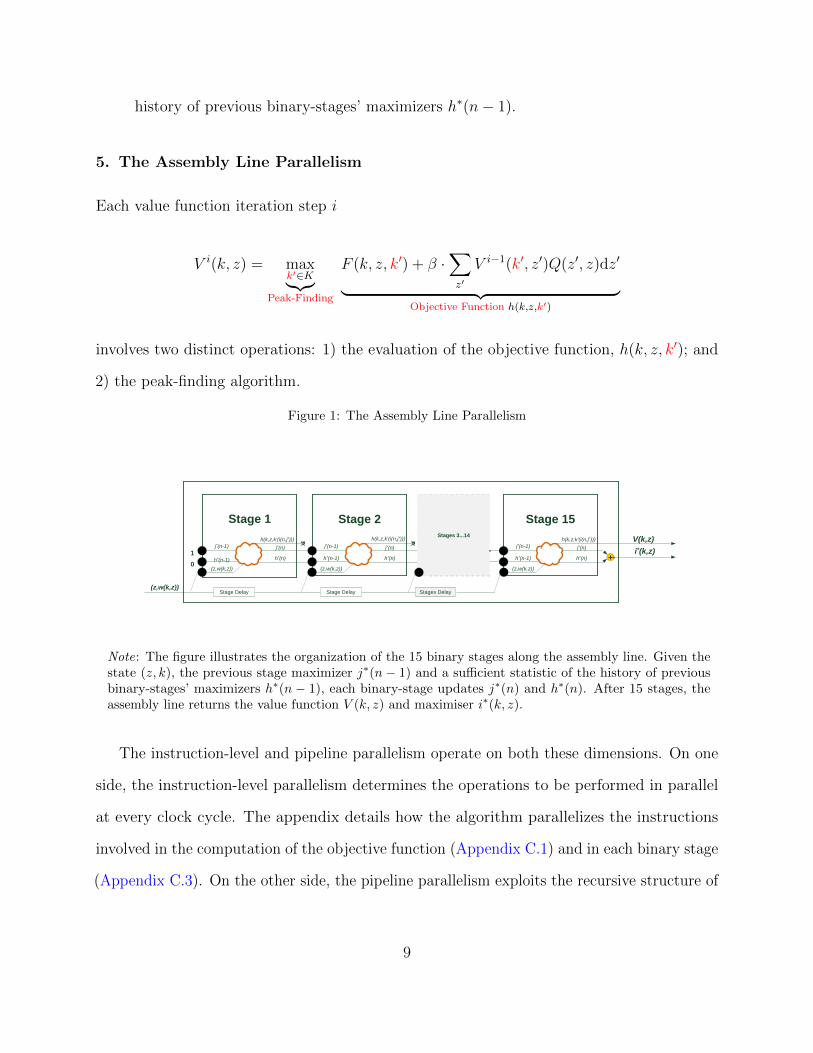
Appendix C.3. The Assembly Line ParallelismThe pipeline parallelism exploits the recursive structure of the binary search algorithm to organize the binarystages around an assembly line, as illustrated in Figure C.6.

Figure C.6: The Assembly Line Parallelism

1

0

j*(n-1)

Stage 2Stages 3...14

Stage 15

+

V(k,z)

(z,w(k,z))Stage Delay Stage Delay Stages Delay

h*(n-1)

(z,w(k,z))

j*(n)

h*(n)

j*(n-1)

h*(n-1)

(z,w(k,z))

h(k,z,k'(i(n,j*)))

j*(n)

h*(n)

j*(n-1)

h*(n-1)

(z,w(k,z))

j*(n)

h*(n)i*(k,z)

Stage 1

h(k,z,k'(i(n,j*)))h(k,z,k'(i(n,j*)))

Note: The figure illustrates the organization of the 15 binary stages along the assembly line. Given thestate (z, k), the previous stage maximizer j∗(n−1) and a sufficient statistic of the history of previous-stagesmaximizers h∗(n − 1), each binary-stage updates j∗(n) and h∗(n). After 15 stages, the assembly linereturns the value function V (k, z) and maximiser i∗(k, z).

For the sake of exposition, let us think at each binary stage as a production team. The 15 teams (binarystages) are assigned:

1. a position n ∈ {1, 2, . . . , 14, 15} in the assembly line;

2. a task, represented by the orange cloud in Figure C.6. To perform their task, teams need threeinputs, as denoted by the three lines entering each orange cloud from the left: the state (k, z) andthe two indexes necessary to select the 3 nth-stage indexes {i(n, j)}j∈{0,1,2,3} at which to evaluate theobjective function {h(k, z, k′(i(n, j)))}j∈{0,1,2,3}. The two indexes are represented by: i) the previousstage maximiser j∗(n− 1) ∈ {0, 1, 2, 3}, as defined in formula (C.6); and ii) a sufficient statistic forthe history of previous winners h∗(n− 1), as defined in formula (C.5).

The task consists in the operations described in the bottom half of Figure C.7). In particular, eachbinary stage: a) uses formula (C.4) to select the 3 nth-stage indexes {i(n, j)}j∈{0,1,2,3} at which toevaluate the objective function {h(k, z, k′(i(n, j)))}j∈{0,1,2,3} (4 in the last stage); b) accesses thememory to retrieve all information needed to calculate the objective function; c) evaluates the objectivefunction at {i(n, j)}j∈{0,1,2,3} as described in Section Appendix C.1, Figure C.4; d) compares theobjective functions and determines the stage maximum and maximiser; e) returns three outputs, asillustrated by the three lines exiting each orange cloud to the right in Figure C.6: e.i) the objectivefunction h(k, z, k′(i(n, j∗))) at j∗; e.ii) the maximiser j∗(n), as defined in (C.6); e.iii) the historyof maximizers at stage n, h∗(n), as defined in (C.5). Importantly, each binary stage performs theseoperations simultaneously, introducing a further layer of instruction-level parallelism.

3. a team of workers. A worker is defined as the logical units in charge of completing a set ofinstructions within a clock cycle. The number of clock cycles required to complete a binary stage(60 Tck) determines the number of workers per team. In each binary stage, workers are assigned a

28

Figure C.7: The Assembly Line Parallelism: Details

Stage (1...14)

1

0

j*(n-1)

Stage 2Stages 3...14

Stage 15

+

V(k,z)

(z,w(k,z))Stage Delay Stage Delay Stages Delay

h*(n-1)

(z,w(k,z))

h(k,z,k'(i(n,j*)))

j*(n)

h*(n)

j*(n-1)

h*(n-1)

(z,w(k,z))

h(k,z,k'(i(n,j*)))

j*(n)

h*(n)

j*(n-1)

h*(n-1)

(z,w(k,z))

h(k,z,k'(i(n,j*)))

j*(n)

h*(n)i*(k,z)

Access Memory

Evaluate Oblective Function Comparison

Select 3 n-th Stage Indexes

i(n,1)

i(n,2)

i(n,3)

Output

Stage 1

Tck

Access Memory

Evaluate Oblective Function ComparisonSelect 3 n-th

Stage Indexes Output

Worker 60Worker 59Worker 2Worker 1 Worker 58Worker 3 Worker 4 Worker 5 Worker 57

605650

Note: The figure illustrates the organization of the Assembly Line Algorithm. The top half of the figureillustrates the 15 binary stages. The bottom half of the figure details the instructions involved at eachstage over the clock cycles.

29

position along an assembly line, as illustrated at the bottom of Figure (C.7). In our implementation,the first 5 workers in each binary stage select the 3 nth-stage indexes and access the memory, the next50 workers evaluate the objective functions as illustrated in Figure C.4; the last 4 workers determinethe stage maximum and maximiser and return the results to the next stage.

30