Discussion Paper No. 450 Nominal or Real? The Impact of ...

Sonderforschungsbereich/Transregio 15 · www.sfbtr15.de

Universität Mannheim · Freie Universität Berlin · Humboldt-Universität zu Berlin · Ludwig-Maximilians-Universität München

Rheinische Friedrich-Wilhelms-Universität Bonn · Zentrum für Europäische Wirtschaftsforschung Mannheim

Speaker: Prof. Dr. Klaus M. Schmidt · Department of Economics · University of Munich · D-80539 Munich,

Phone: +49(89)2180 2250 · Fax: +49(89)2180 3510

*/**/*** University of Bonn

October 15, 2013

Financial support from the Deutsche Forschungsgemeinschaft through SFB/TR 15 is gratefully acknowledged.

Discussion Paper No. 450

Nominal or Real? The Impact of

Regional Price Levels on Satisfaction with Life

Thomas Deckers*

Armin Falk** Hannah Schildberg-Hörisch***

Nominal or Real? The Impact of Regional Price Levels on

Satisfaction with Life

Thomas Deckers∗

University of Bonn

Armin Falk†

University of Bonn

Hannah Schildberg-Horisch‡

University of Bonn

October 15, 2013

Abstract

According to economic theory, real income, i.e., nominal income adjusted for purchasing power,

should be the relevant source of life satisfaction. Previous work, however, has only studied the

impact of inflation adjusted nominal income and not taken into account regional differences

in purchasing power. Therefore, we use a novel data set to study how regional price levels

affect satisfaction with life. The data set comprises about 7 million data points that are used

to construct a price level for each of the 428 administrative districts in Germany. We esti-

mate pooled OLS and ordered probit models that include a comprehensive set of individual

level, time-varying and time-invariant control variables as well as control variables that cap-

ture district heterogeneity other than the price level. Our results show that higher price levels

significantly reduce life satisfaction. Furthermore, we find that a higher price level tends to

induce a larger loss in life satisfaction than a corresponding decrease in nominal income. A

formal test of neutrality of money, however, does not reject neutrality of money. Our results

provide an argument in favor of regional indexation of government transfer payments such as

social welfare benefits.

∗Institute of Applied Microeconomics, University of Bonn, Adenauerallee 24-42, 53113 Bonn, Germany,

[email protected]†Institute of Applied Microeconomics, University of Bonn, Adenauerallee 24-42, 53113 Bonn, Germany,

[email protected]‡Corresponding author, Institute of Applied Microeconomics, University of Bonn, Adenauerallee 24-42, 53113

Bonn, Germany, email: [email protected], phone: 0049-228-739467

1

mailto:[email protected]



Keywords: Life satisfaction, price index, neutrality of money

JEL-Codes: D60, C23, D31

1 Introduction

Among the determinants of life satisfaction, income is of fundamental interest and importance to

economists. Consequently, studies on the effect of income on life satisfaction are abundant. They

range from cross-country studies on the relationship between gross national product and average

reported life satisfaction to analyses of the effect of individual income on individual life satisfaction

(for survey articles see, e.g., Oswald (1997), Frey and Stutzer (2002), Di Tella and MacCulloch

(2006), Clark et al. (2008), Dolan et al. (2008), and Stutzer and Frey (2010)).1 Lacking adequate

data on cross-sectional variation of prices, all research on individual life satisfaction conducted so

far has basically used inflation adjusted nominal income as explanatory variable. According to

microeconomic theory, however, individuals should derive satisfaction from consumption of goods

that they can afford with their income rather than from nominal income. Hence, real income,

i.e., nominal income adjusted for the local price level, is the appropriate concept to measure the

effect of income on life satisfaction.

This paper therefore studies whether differences in local price levels affect individual satisfac-

tion with life once we control for nominal income and local heterogeneity. To this end, we match

two sources of data. The first is a novel and very comprehensive data set on local price levels in

Germany, a price index covering each of Germany’s 428 administrative districts. The price index

reveals substantial price differences within Germany (up to 37%) and is, to our knowledge, unique

at such a disaggregated level. Information used to construct the price index comprises more than

7 million data points. Having information on prices at a more aggregate administrative level (i.e.,

federal states) would not be sufficient for studying the effects of prices on life satisfaction. To illus-

trate, both the cheapest and the most expensive German district are geographically located in the

same federal state. We match our price index data with data from the German Socio-Economic

Panel (SOEP), a household panel survey, which is representative of the German population. It

includes a question on individual life satisfaction, a wide range of control variables, and district

identifiers. To identify the effect of the price level on life satisfaction, we estimate both pooled

OLS and ordered probit models that include a comprehensive set of individual time-variant and

time-invariant characteristics, among many others the ‘Big Five’ personality traits and economic

preferences. Moreover, we control for district characteristics other than the price level that poten-

1Besides studying absolute income, the role of relative income (e.g., Clark and Oswald (1996), Luttmer (2005),

Ferrer-i Carbonell (2005), Fliessbach et al. (2007)) and aspiration income (e.g., Stutzer (2004)) for individual life

satisfaction has been explored.

2

tially influence life satisfaction such as local unemployment rate, local employment rate, average

local household income, distance to the center of the closest large city, and guests-nights per

capita, a proxy for attractiveness of the respective community.

Our main finding is a ‘purchasing power effect’. For a given nominal income, a higher price

level reduces satisfaction with life. The effect sizes are economically relevant. In our main speci-

fication, a 10% increase in the price level is predicted to decrease satisfaction with life by about

0.1 units, where satisfaction with life is measured on a scale from 0 to 10. This effect is roughly

comparable to the decrease in life satisfaction caused by an increase in the distance travelled to

work of about 100 kilometers. Being unemployed instead of full-time employed resembles the

effect size of doubled prices. We perform various robustness checks and extend our analysis to

two subdomains of well-being, in which the difference between nominal and real income is concep-

tually important: individual satisfaction with household income and individual satisfaction with

standard of living. The results further confirm the purchasing power effect. For a given nominal

income, higher local price levels reduce satisfaction with household income and satisfaction with

standard of living at statistically and economically significant rates.

Our results show that not adjusting nationwide payments to regional price differences treats

equals unequally in terms of individual life satisfaction. In this sense, our results provide an

argument in favor of regional indexation of government transfer payments. They also question

country-wide uniform public sector or minimum wages.

Beyond documenting the importance of local price levels for individual well-being, our study

adds to uncovering how people perceive nominal and real quantities. From an economic policy

perspective, perception of real versus nominal terms is, for example, important for determining

optimal inflation rates to be targeted by central banks (Akerlof and Shiller, 2009). Economic

theory usually assumes neutrality of money, i.e., that people think and act in terms of real

quantities and are not guided by nominal quantities. In our case, neutrality of money implies

that a price decrease should affect life satisfaction in the same way as an increase in nominal

income that exactly offsets the price decrease in real income terms. In principle, deviations from

neutrality of money could go in two directions. People could either overreact to changes in nominal

income or to changes in prices.

An overreaction to nominal quantities is usually referred to as money illusion. Fisher (1928)

was the first to suggest that people may exhibit money illusion.2 In contrast, an overreaction to

2Money illusion was basically ignored in economic research until it was again studied by Shafir et al. (1997) who

3

prices would imply that a decrease in prices increases life satisfaction more than a corresponding

increase in disposable nominal income. An overreaction to prices is plausible if prices are more

salient than nominal income. The importance of salience effects is documented in Chetty et al.

(2009), Blumkin et al. (2012), and Finkelstein (2009) who provide evidence that consumers fail

to sufficiently take into account less salient aspects in decision making.3 Income is usually paid

monthly and changes only infrequently. Furthermore, disposable income has many components

that are not very salient such as taxes and government transfer payments. To the contrary, prices

are experienced daily, at every instance of buying.

In contrast to most of the literature, our results on neutrality of money are based on yearly

income data, i.e., large stakes for an individual. In favor of salience effects, our findings document

that people tend to overreact to prices compared to nominal income. In our main specification, the

estimated effect of a change of the price level on overall satisfaction with life is about 66% higher

than the estimated effect of a corresponding change in nominal income. However, a formal test

for neutrality of money, i.e., testing whether the coefficients of the logarithm of nominal income

and the logarithm of the price level differ significantly, does not reject neutrality of money.

The only other study on subjective well-being and price levels we are aware of is Boes et al.

(2007). Their study differs from ours in many respects: the dependent variable, the available

price level data, and methodology. They regress satisfaction with household income on price level

data that was collected in 50 German cities, i.e., not in rural areas (Roos, 2006). Urban price

levels are used to interpolate prices to the level of 13 out of 16 German federal states. Boes

et al. (2007) test if people exhibit money illusion and do not find evidence for it. In contrast,

we discuss and empirically document the effect of the local price level on overall satisfaction with

life, a commonly used proxy for individual utility. Senik (2004) analyzes whether reference group

income influences life satisfaction due to social comparisons or by providing information used to

form expectations about one’s own future income. She constructs ‘real’ income measures by using

report evidence in favor of money illusion using questionnaire and experimental data. Weber et al. (2009) provide

neuroeconomic evidence in favor of money illusion using functional magnetic resonance imaging. Using a laboratory

experiment, Fehr and Tyran (2001) show that even a small extent of money illusion at the individual level may be

sufficient to result in a large aggregate bias after a negative nominal shock.3Chetty et al. (2009) show that consumers underreact to less salient taxes, i.e., taxes that are not included in

price tags. In a lab experiment, Blumkin et al. (2012) find similar evidence. They show that less salient taxes distort

the labor-leisure allocation. Finkelstein (2009) shows that drivers are less aware of tolls that are paid electronically

and, as a consequence, driving is less elastic with respect to tolls that are paid electronically instead of manually.

4

information on regional poverty lines of 38 Russian regions that are provided by the Russian

longitudinal monitoring survey (RLMS) data set. Compared to our data, regional prices refer

to much larger geographical units and are only available for comestible goods that account for

about 9% of components of the price index we use. Luttmer (2005) also analyzes the influence of

reference group income on individual well-being using average earnings in ‘Public Use Microdata

Areas’ of the USA. To control for local characteristics that are both correlated with average local

income and life satisfaction, he uses local housing prices and state fixed effects. Housing prices

correspond to about one fifth of the information our price index contains. He finds that local

housing prices are (insignificantly) negatively correlated with life satisfaction.

The remainder of the paper is organized as follows: section 2 describes both sources of data

and section 3 explains our empirical strategy. Section 4 presents our results and several robustness

checks. We discuss implications of our results and conclude in section 5.

2 Data

We use information on price levels of all 428 German districts (‘Kreise’). Districts constitute

administrative units comprising one or more cities and their surroundings. Districts are the

smallest division of Germany for which it is feasible to collect detailed price data, because in

smaller units some of the products contained in the price index will not be available. The data on

prices at district level have been collected by the German Administrative Office for Architecture

and Comprehensive Regional Planning. Kawka et al. (2009) describe the data set, its collection

and descriptive results on price levels in great detail.

The price index is based on the basket of commodities and the weights attached to each

commodity that are used by the German Federal Statistical Office to calculate the German in-

flation rate. Table 1 lists the most important classes of goods that the basket of commodities

contains. In terms of classes of goods, the price index covers 73.2% of this basket. In particular,

more than 7 million data points on prices of 205 commodities have been collected at the district

level. Commodities range from obvious candidates such as rental rates, electricity prices, or car

prices to such detailed ones as dentist fees, prices for cinema tickets, costs for foreign language

lessons, or entry fees for outdoor swimming pools.

With these data, a price index is constructed that provides an overall price level for each

district. When constructing a price index, a weight needs to be attached to each individual

5

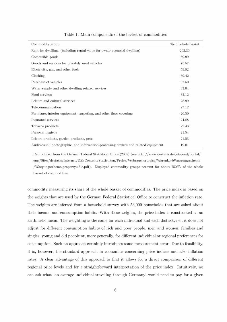
Table 1: Main components of the basket of commodities

Commodity group ‰ of whole basket

Rent for dwellings (including rental value for owner-occupied dwelling) 203.30

Comestible goods 89.99

Goods and services for privately used vehicles 75.57

Electricity, gas, and other fuels 59.82

Clothing 39.42

Purchase of vehicles 37.50

Water supply and other dwelling related services 33.04

Food services 32.12

Leisure and cultural services 28.99

Telecommunication 27.12

Furniture, interior equipment, carpeting, and other floor coverings 26.50

Insurance services 24.88

Tobacco products 22.43

Personal hygiene 21.54

Leisure products, garden products, pets 21.53

Audiovisual, photographic, and information-processing devices and related equipment 19.01

Reproduced from the German Federal Statistical Office (2005) (see http://www.destatis.de/jetspeed/portal/

cms/Sites/destatis/Internet/DE/Content/Statistiken/Preise/Verbraucherpreise/WarenkorbWaegungsschema

/Waegungsschema,property=file.pdf). Displayed commodity groups account for about 750 ‰ of the whole

basket of commodities.

commodity measuring its share of the whole basket of commodities. The price index is based on

the weights that are used by the German Federal Statistical Office to construct the inflation rate.

The weights are inferred from a household survey with 53,000 households that are asked about

their income and consumption habits. With these weights, the price index is constructed as an

arithmetic mean. The weighting is the same for each individual and each district, i.e., it does not

adjust for different consumption habits of rich and poor people, men and women, families and

singles, young and old people or, more generally, for different individual or regional preferences for

consumption. Such an approach certainly introduces some measurement error. Due to feasibility,

it is, however, the standard approach in economics concerning price indices and also inflation

rates. A clear advantage of this approach is that it allows for a direct comparison of different

regional price levels and for a straightforward interpretation of the price index. Intuitively, we

can ask what ‘an average individual traveling through Germany’ would need to pay for a given

6

consumption bundle in each district. Since collecting such comprehensive data cannot be managed

in a single year, the data were gathered in the years 2004 to 2009, with most of the data, roughly

85%, being collected from 2006 to 2008. The data are used to build a single time-invariant price

level for each district.

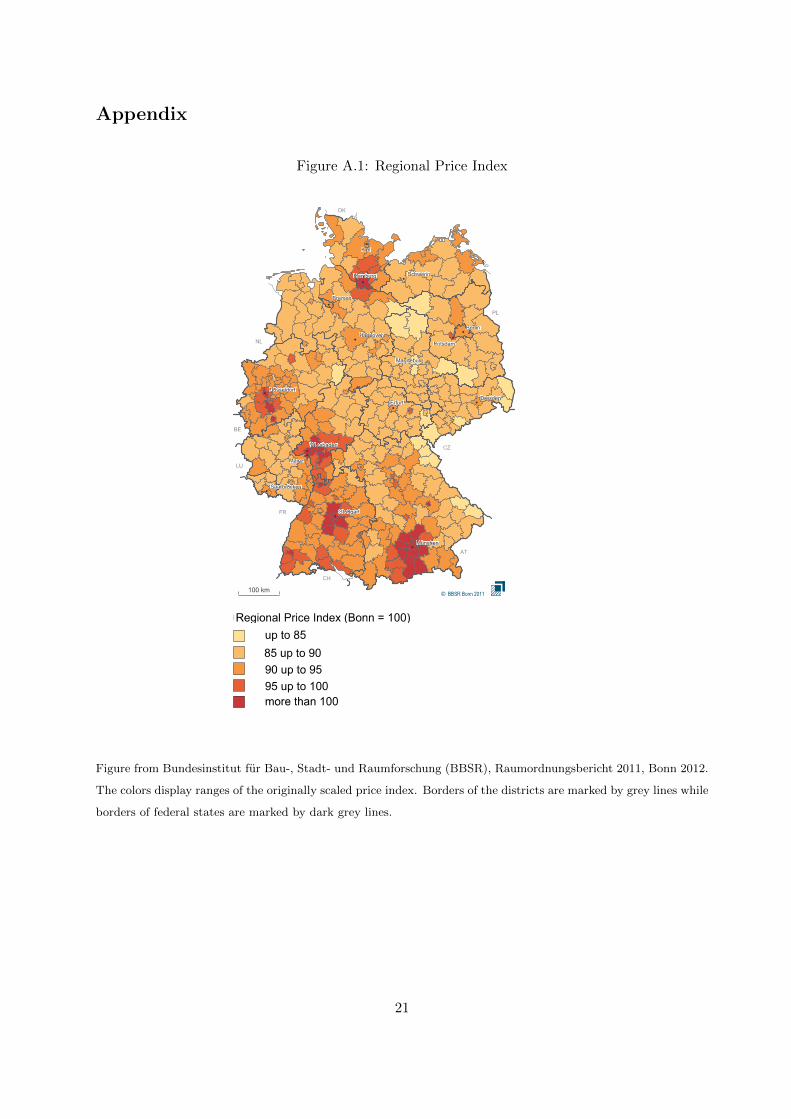
The price index uses the district of the former German capital Bonn as baseline (100 points).

The cheapest district is Tirschenreuth in the federal state of Bavaria with 83.37 points, while

Munich with 114.40 points (also in Bavaria) is the most expensive district. Hence, the most

expensive district is 37% more expensive than the cheapest, revealing a substantial price difference

within Germany. Figure A.1 in the Appendix shows a map of Germany indicating the price level

of each district. Three observations are worth mentioning: price levels are generally lower in East

than in West Germany and lower in Northern than in Southern Germany. Moreover, urban areas

are more expensive than rural ones.

To obtain a measure of prices that accounts for both cross-sectional variation of prices at

the district level and variation of prices over time, we multiply district specific price levels with

inflation rates using 2006 as baseline year. The smallest geographical unit for which regional

inflation rates are available in Germany is at the level of the 16 federal states.4

We match the price index data and data from the SOEP using district identifiers.5 The SOEP

is a representative panel study of German households that started in 1984. We use five waves

from 2004 to 2008.6 In each wave, about 22,000 individuals in 12,000 households are interviewed.

Data cover a wide range of topics such as individual attitudes, preferences, and personality, job

characteristics, employment status and income, family characteristics, health status, and living

conditions. Schupp and Wagner (2002) and Wagner et al. (2007) provide an in-depth description

of the SOEP.

Since the first wave in 1984 participants are asked about their satisfaction with life on an

4From 2004 to 2008, 13 out of a total of 16 federal states report inflation rates for each year. For the federal state

of Bremen, only the value for 2004 is missing. The federal states Hamburg and Schleswig-Holstein do not report

own inflation rates in any year. For all missings, we interpolate the state level inflation rates with the German wide

inflation rate of the corresponding year.5Due to data privacy protection rules, working with the SOEP data at district level requires a special mode of

online access to the SOEP data, SOEPremote.6We cannot comprehensively match the price data to SOEP data from 2009 onwards. In 2009, some district

boundaries were restructured. The new district boundaries are only reflected in the SOEP data, but not in the

price index data.

7

eleven point Likert scale, which constitutes our main dependent variable. The life satisfaction

question reads: “How satisfied are you with your life, all things considered?”. Life satisfaction

is often used as a measure for individual welfare or utility.7 It is also gaining importance as

an evaluation tool for economic policy. For example, in 2008, French President Nicholas Sarkozy

asked a commission of economists to develop better measures for economic performance and social

progress than, for example, GDP. In their report, the so called ‘Sarkozy commission’ notes that

“... the time is ripe for our measurement system to shift emphasis from measuring economic

production to measuring people’s well-being.” (p.12, Stiglitz et al. (2009)).

As alternative dependent variables, we use individual satisfaction with household income and

individual satisfaction with standard of living. They are elicited in the following SOEP questions:

“How satisfied are you with your household income?” and “Overall, how satisfied are you with

your standard of living?”. Satisfaction with household income is available from 2004 to 2008,

while satisfaction with standard of living is only available from 2004 to 2006. Both questions

use an eleven point Likert scale. Compared to general satisfaction with life, satisfaction with

household income or standard of living is smaller in scope and less apt as a proxy for overall

individual utility. However, they are even more closely linked to real (as opposed to nominal)

income. Thus, the two alternative dependent variables will be useful to provide further evidence

on how regional price levels affect well-being.

Besides a district’s price level, nominal income is the main explanatory variable. We mea-

sure nominal income by household disposable nominal income, i.e., after tax household income

including all kinds of government transfer income.8 Instead of calculating equivalence income, we

control for the logarithm of persons living in the household.

Additionally, we use a very comprehensive and well-established set of control variables at both

individual and district level. The time-varying control variables at the individual level are age, age

squared, dummies for marital status (married, separated, divorced, widowed; single as omitted

category), dummies for employment status (employed full-time, employed part-time, maternity

leave, non-participant; unemployed as omitted category), years of education, a binary variable

indicating whether an individual is disabled, a continuous variable indicating the official level of

7For a detailed discussion on the relationship between satisfaction with life and utility see, for example, Clark

et al. (2008) and Oswald (2008).8We exclude about 60 observations with incomes above 500,000 Euro to avoid results being influenced by extreme

outliers. Including them does not change our results.

8

disability, the number of children in the household, and the distance travelled to the workplace

in kilometers.

Furthermore, we use a comprehensive set of individual specific, time-invariant control vari-

ables. We include dummies for gender, German nationality, whether an individual describes

himself as religious, and information on the political orientation of a person, which was elicited

in SOEP wave 2005 on a scale from 0 (extreme left wing) to 10 (extreme right wing). Most

importantly, we control for an individual’s personality, economic preferences, and beliefs. Becker

et al. (2012) show that concepts from psychology and economics should be combined when mod-

eling individual differences. Using this approach, a large fraction of the variance in outcomes

such as life satisfaction can be explained. Building on research in personality psychology, our

control variables encompass the so called “Big Five”, which are five superordinated character

traits into which most of the subordinated character traits can be mapped (Costa and McCrae,

1992). The Big Five are openness to experience, conscientiousness, extraversion, agreeableness,

and neuroticism.9 For each trait, we use standardized questionnaire measures that were elicited in

the 2005 wave of the SOEP. A further important personality trait is the so called locus of control

(Rotter, 1966). Locus of control measures the extent to which people think they are in control

of events in their life. Our measure of locus of control uses standardized questionnaire measures

from the 2005 wave of the SOEP. In economics, individual differences are commonly modeled by

differences in preferences and beliefs. Important preferences are the preference for risk and time

as well as social preferences (altruism, positive and negative reciprocity). An important belief is

trust. Except for time preferences, all preferences and beliefs mentioned above were elicited at

least once in the SOEP between 2004 to 2008. Whenever we have multiple measures for a given

concept, we use the average to reduce measurement error. All measures are standardized.

To model district characteristics other than the price level that could both influence satisfac-

tion with life and be correlated with the price level, we also include control variables at district

level. The time-varying control variables mainly encompass macroeconomic variables that cap-

ture the current economic situation at district level: the average unemployment rate, the average

employment rate in jobs subject to social security contributions, and the logarithm of the average

household income. The time-invariant variables include the district size in square kilometers,

the distance to the center of the closest large city (measured at individual level in 2004), and

the number of guest-nights per capita in 2007 that proxy local attractiveness in terms of natural

9For a detailed description of the Big Five see, e.g., Borghans et al. (2008).

9

beauty or cultural facilities.

3 Empirical Strategy

We estimate a pooled OLS model with error terms clustered at district level for individual i’s

satisfaction with life in district j and a given year t, Hijt:

Hijt = β0 + β1ln(Nit) + β2ln(pjt) + β3ln(sit) + x′itγ1 + c′iγ2 + d′jtγ3 + d′jγ4 + γ5tht + εijt

Nit is nominal income. pjt is the price index that captures cross-sectional variation of prices across

districts and variation of prices over time. sit is the number of persons living in the household,

xit is a vector including individual specific, time-varying control variables, ci is a vector of time-

invariant individual characteristics. djt and dj are vectors of time-variant and time-invariant

control variables at district level, ht is a year dummy, β0 is a constant term, and εijt the error

term.

Our primary research question is whether, for a given nominal income, differences in regional

price levels affect individual satisfaction with life, i.e., whether β2 is significantly different from

zero. In addition, the specification at hand allows for a direct test of neutrality of money by

testing whether β1 is significantly different from β2 in absolute value. According to economic

theory, real income, i.e., nominal income adjusted for the regional price level, as opposed to pure

nominal income should be the relevant source of satisfaction with life. Consequently, the two

coefficients β1 and β2 should be of the same size in absolute terms. Assuming that β1 is positive

and β2 is negative, a β1 that is larger than |β2| would indicate that people exhibit nominal illusion.

If |β2| were larger than β1, the average individual would overreact to prices compared to nominal

income, i.e., would suffer more from a price increase than it would suffer from a corresponding

decrease in nominal income.

With the data at hand, it is not feasible to identify how regional price differences affect

satisfaction with life by estimating an individual and / or district fixed effects model with ln(pjt)

as key explanatory variable. Since ln(pjt) = ln(pj) + ln(inflationt), the price index consists

of a time-invariant part, ln(pj), that contains cross-sectional price variation and a time-variant

part, the inflation rate. In a fixed effects regression using individual or district fixed effects, the

time-invariant part of the price level, ln(pj), does not contribute to identifying the coefficient of

ln(pjt). The coefficient of ln(pjt) would only be identified via the inflation rate. Thus, it would

not contain any information on how regional price levels influence satisfaction with life.

10

This argument neglects that individuals who move from one district to another provide an

alternative source of variation in local prices that could potentially be used to identify the effect

of the regional price level on individual satisfaction with life. However, movers constitute only

a very small group of our sample. Furthermore, movers are likely to be a peculiar subset of

the population, experiencing particularly strong shocks to life satisfaction caused by shocks to

unobserved heterogeneity, e.g., frequent reasons for moving are changing the job or moving to

live together with the partner. Thus, we are reluctant to generalize results that are based on

movers only to the population as a whole and exclude movers from our main specification. In

fact, estimating a fixed effects specification that uses only observations on movers estimates the

impact of income on happiness to be negative which is in stark contrast to all existing literature

(see, e.g., the survey of Dolan et al. (2008)).

Since we cannot include individual or district fixed effects, we use a very comprehensive set

of time-invariant individual and district characteristics as regressors to explicitly model time-

invariant sources of heterogeneity in overall satisfaction with life as advocated by, e.g., Ferrer-i-

Carbonell and Frijters (2004).

4 Results

We first present and discuss the effect of cross-sectional variation of prices on overall satisfaction

with life, before studying how cross-sectional variation of prices affects individual satisfaction

with household income and individual satisfaction with standard of living, the two alternative

dependent variables we use.

4.1 Results for overall satisfaction with life

Table 2 displays the main estimation results. In all specifications, the logarithm of nominal income

has a statistically significant, positive influence on satisfaction with life (p < 0.01). Moreover,

all specifications document economies of scale at the household level as the coefficient of the

logarithm of household size (p < 0.01) is smaller than the coefficient of the logarithm of nominal

income in absolute terms.

11

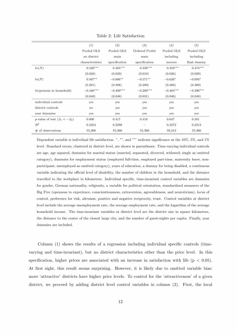
Table 2: Life Satisfaction

(1) (2) (3) (4) (5)

Pooled OLS Pooled OLS Ordered Probit Pooled OLS Pooled OLS

no district main main including including

characteristics specification specification movers East dummy

ln(N) 0.520∗∗∗ 0.485∗∗∗ 0.338∗∗∗ 0.458∗∗∗ 0.474∗∗∗

(0.028) (0.029) (0.019) (0.026) (0.029)

ln(P ) 0.567∗∗ −0.806∗∗ −0.571∗∗ −0.626∗ −0.693∗

(0.281) (0.398) (0.290) (0.369) (0.399)

ln(persons in household) −0.446∗∗∗ −0.409∗∗∗ −0.290∗∗∗ −0.404∗∗∗ −0.396∗∗∗

(0.048) (0.048) (0.031) (0.046) (0.048)

individual controls yes yes yes yes yes

district controls no yes yes yes yes

year dummies yes yes yes yes yes

p-value of test (β1 = −β2) 0.000 0.417 0.418 0.647 0.581

R2 0.2254 0.2298 – 0.2272 0.2313

# of observations 55,366 55,366 55,366 59,212 55,366

Dependent variable is individual life satisfaction. ∗, ∗∗, and ∗∗∗ indicate significance at the 10%, 5%, and 1%

level. Standard errors, clustered at district level, are shown in parentheses. Time-varying individual controls

are age, age squared, dummies for marital status (married, separated, divorced, widowed; single as omitted

category), dummies for employment status (employed full-time, employed part-time, maternity leave, non-

participant; unemployed as omitted category), years of education, a dummy for being disabled, a continuous

variable indicating the official level of disability, the number of children in the household, and the distance

travelled to the workplace in kilometers. Individual specific, time-invariant control variables are dummies

for gender, German nationality, religiosity, a variable for political orientation, standardized measures of the

Big Five (openness to experience, conscientiousness, extraversion, agreeableness, and neuroticism), locus of

control, preference for risk, altruism, positive and negative reciprocity, trust. Control variables at district

level include the average unemployment rate, the average employment rate, and the logarithm of the average

household income. The time-invariant variables at district level are the district size in square kilometers,

the distance to the center of the closest large city, and the number of guest-nights per capita. Finally, year

dummies are included.

Column (1) shows the results of a regression including individual specific controls (time-

varying and time-invariant), but no district characteristics other than the price level. In this

specification, higher prices are associated with an increase in satisfaction with life (p < 0.05).

At first sight, this result seems surprising. However, it is likely due to omitted variable bias:

more ‘attractive’ districts have higher price levels. To control for the ‘attractiveness’ of a given

district, we proceed by adding district level control variables in column (2). First, the local

12

unemployment rate, the employment rate, and the average district household income describe the

current economic situation at district level. Second, the district’s size and the distance to the

center of the closest large city are proxies for how rural or urban a given district is and thus also

for its infrastructure. Finally, the number of guest-nights per capita proxies local attractiveness

in terms of natural beauty or cultural facilities.

Column (2) presents the results of our main specification.10 There are two key insights.

First, for a given nominal income, higher local prices decrease individual satisfaction with life (p

< 0.05). A 10% increase in the price level is predicted to decrease satisfaction with life by 0.08

units, where satisfaction with life is measured at a 11 point Likert scale. To get a better intuition

for the magnitude of the price level effect on life satisfaction, we compare the coefficient of the

price level with coefficient of other explanatory variables. For example, an increase of the price

level by around 8% decreases life satisfaction as much as an increase in the distance travelled to

work of around 100 kilometers. Being unemployed instead of full-time employed resembles the

effect size of a doubling of prices.

Second, our results do not reject neutrality of money. Testing whether the coefficient of

nominal income, β1, is significantly different from the coefficient of the price level, β2, in absolute

terms yields p = 0.42. However, in absolute terms, the coefficient of the logarithm of the price

level is 66% larger than the coefficient of the logarithm of nominal income, indicating that people

have the tendency to react stronger to changes in prices than to corresponding changes in nominal

income. For example, while a 10% increase in the price level is predicted to decrease satisfaction

with life by 0.08 units, a 10% decrease in nominal income is predicted to reduce satisfaction with

life by only 0.05 units. Salience effects (Chetty et al. (2009), Blumkin et al. (2012), Finkelstein

(2009)) offer a possible explanation for a larger impact of prices than of nominal income on

satisfaction if prices are more salient than disposable income. This seems likely. Many components

of disposable income might be less salient, e.g., taxes and government transfer payments, and, for

most people, income changes are relatively rare events. In contrast, prices and price changes are

experienced frequently, prices at every instance of buying.

We check the robustness of our main specification in various ways. First, in column (3), we

take into account the ordinal nature of our dependent variable by estimating an ordered probit

10Table A.1 in the Appendix displays all estimated coefficients of the main specification. It documents that,

in general, the estimated coefficients of our control variables are well in line with the existing literature. The

time-invariant personality traits and economic preferences contribute significantly to explaining life satisfaction.

13

model. Using the ordinal model, the coefficient of the price level remains significantly negative

(p < 0.05). As a second robustness check, in column (4), we add observations from all movers

to the sample. As noted before, movers constitute a peculiar subgroup that, when analyzed

separately in a fixed-effects framework, show a negative relationship between nominal income and

satisfaction with life. However, including movers in our sample, results stay qualitatively the same.

For a given nominal income, a higher price level is still predicted to decrease satisfaction with life

(p < 0.1). Again, we do not reject neutrality of money. Finally, we include an additional dummy

variable indicating whether a district lies in East or West Germany in column (5). Frijters et al.

(2004) document that life satisfaction in East Germany is generally lower than in West Germany.

Our district level explanatory variables should already capture a large share of differences between

East and West Germany that still exist and affect satisfaction with life, such as differences in

economic conditions. Including an East / West dummy allows controlling for potential further

differences between East and West Germany. Once more, our results are stable and document

that, for a given nominal income, higher prices reduce satisfaction with life (p < 0.1). Again, we

do not reject neutrality of money (p = 0.58).

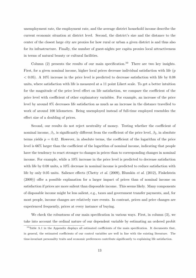
4.2 Results for satisfaction with household income and satisfaction with stan-

dard of living

In order to obtain further evidence on how the local price level affects individual well-being,

we investigate the influence of the local price level on satisfaction with household income and

satisfaction with standard of living. Real income seems to be a driving force for both subdomaines

of individual well-being. In contrast, it is a well-established result that income has a significant

impact on overall satisfaction with life, but, compared to other explanatory variables such as

unemployment or health, the role of income is relatively small. Consequently, we hypothesize

that the coefficients of nominal income and the local price level are larger in those two domains

than for overall satisfaction with life.

14

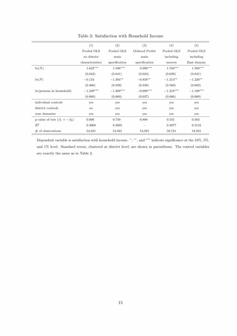
Table 3: Satisfaction with Household Income

(1) (2) (3) (4) (5)




ln(N) 1.622∗∗∗ 1.586∗∗∗ 0.906∗∗∗ 1.550∗∗∗ 1.569∗∗∗

(0.042) (0.041) (0.024) (0.039) (0.041)

ln(P ) −0.134 −1.394∗∗ −0.858∗∗ −1.213∗∗ −1.220∗∗

(0.360) (0.599) (0.338) (0.569) (0.602)


(0.069) (0.069) (0.037) (0.066) (0.069)




p-value of test (β1 = −β2) 0.000 0.749 0.888 0.555 0.563

R2 0.3068 0.3095 – 0.3077 0.3116

# of observations 54,921 54,921 54,921 58,721 54,921

Dependent variable is satisfaction with household income. ∗, ∗∗, and ∗∗∗ indicate significance at the 10%, 5%,

and 1% level. Standard errors, clustered at district level, are shown in parentheses. The control variables

are exactly the same as in Table 2.

15

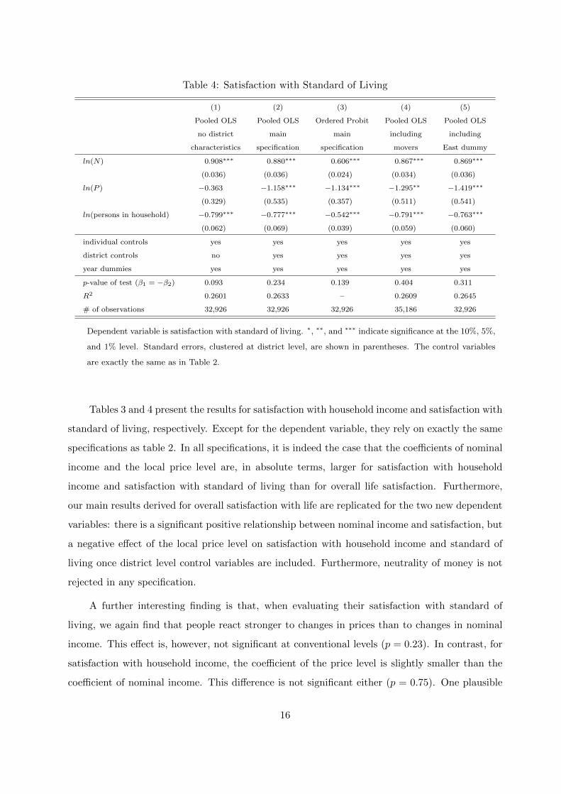
Table 4: Satisfaction with Standard of Living

(1) (2) (3) (4) (5)




ln(N) 0.908∗∗∗ 0.880∗∗∗ 0.606∗∗∗ 0.867∗∗∗ 0.869∗∗∗

(0.036) (0.036) (0.024) (0.034) (0.036)

ln(P ) −0.363 −1.158∗∗∗ −1.134∗∗∗ −1.295∗∗ −1.419∗∗∗

(0.329) (0.535) (0.357) (0.511) (0.541)


(0.062) (0.069) (0.039) (0.059) (0.060)




p-value of test (β1 = −β2) 0.093 0.234 0.139 0.404 0.311

R2 0.2601 0.2633 – 0.2609 0.2645

# of observations 32,926 32,926 32,926 35,186 32,926

Dependent variable is satisfaction with standard of living. ∗, ∗∗, and ∗∗∗ indicate significance at the 10%, 5%,

and 1% level. Standard errors, clustered at district level, are shown in parentheses. The control variables

are exactly the same as in Table 2.

Tables 3 and 4 present the results for satisfaction with household income and satisfaction with

standard of living, respectively. Except for the dependent variable, they rely on exactly the same

specifications as table 2. In all specifications, it is indeed the case that the coefficients of nominal

income and the local price level are, in absolute terms, larger for satisfaction with household

income and satisfaction with standard of living than for overall life satisfaction. Furthermore,

our main results derived for overall satisfaction with life are replicated for the two new dependent

variables: there is a significant positive relationship between nominal income and satisfaction, but

a negative effect of the local price level on satisfaction with household income and standard of

living once district level control variables are included. Furthermore, neutrality of money is not

rejected in any specification.

A further interesting finding is that, when evaluating their satisfaction with standard of

living, we again find that people react stronger to changes in prices than to changes in nominal

income. This effect is, however, not significant at conventional levels (p = 0.23). In contrast, for

satisfaction with household income, the coefficient of the price level is slightly smaller than the

coefficient of nominal income. This difference is not significant either (p = 0.75). One plausible

16

explanation could again be salience effects: if people are directly asked about their satisfaction

with household income, nominal income might be particularly salient.

5 Discussion

We have used a novel and very comprehensive data set on local price levels in Germany to study

whether cross-sectional variation in price levels affects satisfaction with life once nominal income

is controlled for. Our results show that information on price levels matters when analyzing

satisfaction with life. We find that people exhibit significantly lower life satisfaction when living

in a more expensive region. The effect of an increase in the price level on life satisfaction is also

economically significant: A 10% increase in the price level decreases satisfaction with life by 0.08

units on a scale ranging from 0 to 10. Moreover, although a marginal price decrease is estimated to

have a 66% stronger impact on life satisfaction than a corresponding increase in nominal income,

this discrepancy is not large enough to reject neutrality of money. The result that, for a given

nominal income, a higher price level reduces individual well-being also extends to subdomains

of well-being, in particular satisfaction with household income and satisfaction with standard of

living.

Our results are of relevance for advising policy, in particular if policy aims at treating equals

equally. In that sense, our findings call for a regional indexation of government transfer payments,

such as the US Supplemental Security Income (SSI), unemployment benefits, or social welfare

benefits. Our results also put country-wide uniform public sector or minimum wages into question.

In all examples, not adjusting nationwide payments to regional price differences risks treating

equals unequally in terms of individual satisfaction with life.11

We believe that the price index data employed in this paper offer lots of scope for future

research. Relevant questions that require detailed information on local price levels comprise, e.g.,

the effect of the price level on whether wages are perceived as fair, how job search activity or

investments in human capital depend on regional price differences, and whether local price levels

affect migration within a country.

11Of course, the validity of these arguments rests on a ceteris paribus assumption, i.e., groups who get compensated

for differences in the price level are assumed to be small enough for a change in their nominal income not to affect

the local price level.

17

Acknowledgements

We thank Rupert Kawka for providing the price index data and for valuable comments while

working with them and Christoph Hanck, Andrew Oswald, Alois Stutzer and Rainer Winkel-

mann for insightful comments. Financial support from the German Science Foundation (that

did not influence study design or interpretation of the results) through SFB-TR 15 is gratefully

acknowledged.

18

References

Akerlof G, Shiller R. 2009. Animal Spirits: How Human Psychology Drives the Economy, and Why it Matters for

Global Capitalism. Princeton: Princeton University Press.

Becker A, Deckers T, Dohmen T, Falk A, Kosse F. 2012. The Relationship Between Economic Preferences and

Psychological Personality Measures. Annual Review of Economics 4: 453–478.

Blumkin T, Ruffle B, Ganun Y. 2012. Are Income and Consumption Taxes Ever Really Equivalent? Evidence from

a Real-Effort Experiment with Real Goods. European Economic Review 56: 1200–1219.

Boes S, Lipp M, Winkelmann R. 2007. Money Illusion under Test. Economics Letters 94: 332–337.

Borghans L, Duckworth AL, Heckman JJ, ter Weel B. 2008. The Economics and Psychology of Personality Traits.

Journal of Human Resources 43: 972–1059.

Chetty R, Looney A, Kroft K. 2009. Salience and Taxation: Theory and Evidence. American Economic Review

99: 1145–1177.

Clark AE, Frijters P, Shields MA. 2008. Relative Income, Happiness, and Utility: An Explanation for the Easterlin

Paradox and Other Puzzles. Journal of Economic Literature 46: 95–144.

Clark AE, Oswald AJ. 1996. Satisfaction and comparison income. Journal of Public Economics 61: 359–381.

Costa P, McCrae R. 1992. Revised NEO Personality Inventory (NEO PI-R) and NEO Five-Factor Inventory (NEO-

FFI). Odessa, FL, Psychological Assessment Resources.

Di Tella R, MacCulloch R. 2006. Some uses of happiness data in economics. The Journal of Economic Perspectives

20: 25–46.

Dolan P, Peasgood T, White M. 2008. Do we really know what makes us happy? A review of the economic literature

on the factors associated with subjective well-being. Journal of Economic Psychology 29: 94–122.

Fehr E, Tyran JR. 2001. Does money illusion matter? The American Economic Review 91: 1239–1262.

Ferrer-i Carbonell A. 2005. Income and Well-Being: An Empirical Analysis of the Comparison Income Effect.

Journal of Public Economics 89: 997–1019.

Ferrer-i-Carbonell A, Frijters P. 2004. How important is methodology for the estimates of the determinants of

happiness? The Economic Journal 114: 641–659.

Finkelstein A. 2009. E-ZTax: Tax Salience and Tax Rates. The Quarterly Journal of Economics 124: 969—1010.

Fisher I. 1928. The Money Illusion. New York: Adelphi.

Fliessbach K, Weber B, Trautner P, Dohmen T, Sunde U, Elger CE, Falk A. 2007. Social Comparison Affects

Reward-Related Brain Activity in the Human Ventral Striatum. Science 318: 1305—1308.

Frey BS, Stutzer A. 2002. What Can Economists Learn from Happiness Research? Journal of Economic Literature

40: 402–435.

Frijters P, Haisken-DeNew JP, Shields MA. 2004. Money does matter! Evidence from increasing real income and

life satisfaction in east germany following reunification. American Economic Review 94: 730–740.

Kawka R, Beisswenger S, Costa G, Kemmerling H, Muller S, Putz T, Schmidt H, Schmidt S, Trimborn M. 2009.

Regionaler Preisindex, Berichte Band 30. Bundesinstitut fur Bau-, Stadt- und Raumforschung, Bonn.

Luttmer E. 2005. Neighbors as Negatives: Relative Earnings and Well-Being. Quarterly Journal of Economics 120:

963—1002.

Oswald A. 1997. Happiness and economic performance. The Economic Journal 107: 1815–1831.

19

Oswald A. 2008. On the curvature of the reporting function from objective reality to subjective feelings. Economic

Letters 100: 369–372.

Roos MWM. 2006. Regional Price Levels in Germany. Applied Economics 38: 1553–1566.

Rotter J. 1966. Generalized expectancies for internal versus external control of reinforcement. Psychological Mono-

graphs 80: 1–28.

Schupp J, Wagner GG. 2002. Maintenance of and Innovation in Long-Term Panel Studies The Case of the German

Socio-economic panel (GSOEP). Allgemeines Statistisches Archiv 86: 163–175.

Senik C. 2004. When Information Dominates Comparison: Learning from Russian Subjective Panel Data. Journal

of Public Economics 88: 2099–2123.

Shafir E, Diamond P, Tversky A. 1997. Money illsuion. The Quarterly Journal Of Economics 112: 341–374.

Stiglitz J, Sen A, Fitoussi JP, Agarwal B, Arrow KJ, Atkinson AB, Bourguignon F, Cotis JP, Deaton AS, Dervis

K, Fleurbaey M, Folbre N, Gadrey J, Giovannini E, Guesnerie R, Heckman JJ, Heal G, Henry C, Kahneman

D, Krueger AB, Oswald AJ, Putnam RD, Stern N, Sunstein C, Weil P. 2009. Report by the Comission on the

Measurement of Economic Performance and Social Progress. www.stiglitz-sen-fitoussi.fr.

Stutzer A. 2004. The role of income aspirations in individual happiness. Journal of Economic Behavior and Orga-

nization 54: 89–109.

Stutzer A, Frey BS. 2010. Recent Advances in the Economics of Individual Subjective Well-Being. Social research:

An International Quarterly 77: 679–714.

Wagner GG, Frick JR, Schupp J. 2007. The German Socio-Economic Panel Study (SOEP) - Evolution, Scope and

Enhancements. SOEPpapers 1, DIW Berlin, The German Socio-Economic Panel (SOEP) .

Weber B, Rangel A, Wibral M, Falk A. 2009. The medial prefrontal cortex exhibits money illusion. PNAS 106:

5025–5028.

20

Appendix

Figure A.1: Regional Price Index

Figure from Bundesinstitut fur Bau-, Stadt- und Raumforschung (BBSR), Raumordnungsbericht 2011, Bonn 2012.

The colors display ranges of the originally scaled price index. Borders of the districts are marked by grey lines while

borders of federal states are marked by dark grey lines.

21

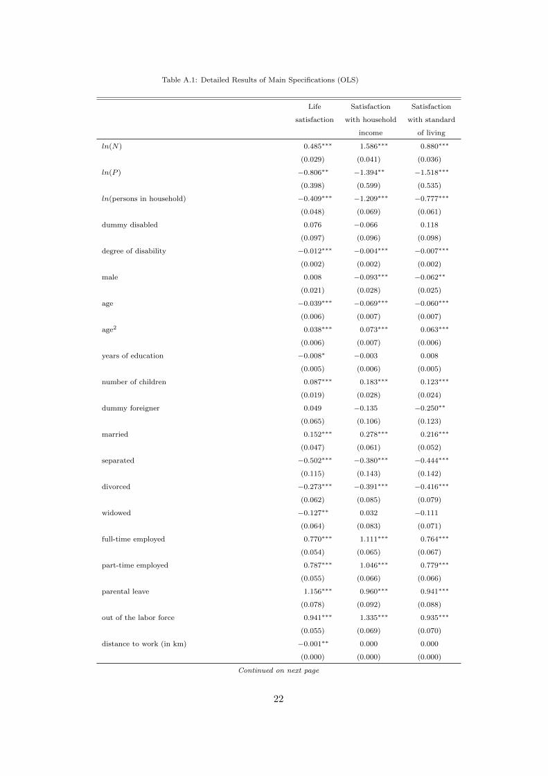
Table A.1: Detailed Results of Main Specifications (OLS)

Life Satisfaction Satisfaction

satisfaction with household with standard

income of living

ln(N) 0.485∗∗∗ 1.586∗∗∗ 0.880∗∗∗

(0.029) (0.041) (0.036)

ln(P ) −0.806∗∗ −1.394∗∗ −1.518∗∗∗

(0.398) (0.599) (0.535)

ln(persons in household) −0.409∗∗∗ −1.209∗∗∗ −0.777∗∗∗

(0.048) (0.069) (0.061)

dummy disabled 0.076 −0.066 0.118

(0.097) (0.096) (0.098)

degree of disability −0.012∗∗∗ −0.004∗∗∗ −0.007∗∗∗

(0.002) (0.002) (0.002)

male 0.008 −0.093∗∗∗ −0.062∗∗

(0.021) (0.028) (0.025)

age −0.039∗∗∗ −0.069∗∗∗ −0.060∗∗∗

(0.006) (0.007) (0.007)

age2 0.038∗∗∗ 0.073∗∗∗ 0.063∗∗∗

(0.006) (0.007) (0.006)

years of education −0.008∗ −0.003 0.008

(0.005) (0.006) (0.005)

number of children 0.087∗∗∗ 0.183∗∗∗ 0.123∗∗∗

(0.019) (0.028) (0.024)

dummy foreigner 0.049 −0.135 −0.250∗∗

(0.065) (0.106) (0.123)

married 0.152∗∗∗ 0.278∗∗∗ 0.216∗∗∗

(0.047) (0.061) (0.052)

separated −0.502∗∗∗ −0.380∗∗∗ −0.444∗∗∗

(0.115) (0.143) (0.142)

divorced −0.273∗∗∗ −0.391∗∗∗ −0.416∗∗∗

(0.062) (0.085) (0.079)

widowed −0.127∗∗ 0.032 −0.111

(0.064) (0.083) (0.071)

full-time employed 0.770∗∗∗ 1.111∗∗∗ 0.764∗∗∗

(0.054) (0.065) (0.067)

part-time employed 0.787∗∗∗ 1.046∗∗∗ 0.779∗∗∗

(0.055) (0.066) (0.066)

parental leave 1.156∗∗∗ 0.960∗∗∗ 0.941∗∗∗

(0.078) (0.092) (0.088)

out of the labor force 0.941∗∗∗ 1.335∗∗∗ 0.935∗∗∗

(0.055) (0.069) (0.070)

distance to work (in km) −0.001∗∗ 0.000 0.000

(0.000) (0.000) (0.000)

Continued on next page

22

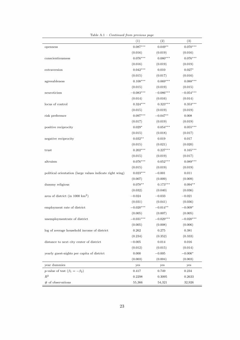
Table A.1 – Continued from previous page

(1) (2) (3)

openness 0.087∗∗∗ 0.049∗∗ 0.070∗∗∗

(0.016) (0.019) (0.016)

conscientiousness 0.076∗∗∗ 0.080∗∗∗ 0.076∗∗∗

(0.016) (0.019) (0.019)

extraversion 0.042∗∗∗ 0.010 0.027∗

(0.015) (0.017) (0.016)

agreeableness 0.108∗∗∗ 0.069∗∗∗ 0.088∗∗∗

(0.015) (0.019) (0.015)

neuroticism −0.083∗∗∗ −0.086∗∗∗ −0.054∗∗∗

(0.014) (0.016) (0.014)

locus of control 0.324∗∗∗ 0.323∗∗∗ 0.353∗∗∗

(0.015) (0.019) (0.019)

risk preference 0.097∗∗∗ −0.047∗∗ 0.008

(0.017) (0.019) (0.019)

positive reciprocity 0.029∗ 0.054∗∗∗ 0.055∗∗∗

(0.015) (0.018) (0.017)

negative reciprocity 0.032∗∗ 0.019 0.017

(0.015) (0.021) (0.020)

trust 0.202∗∗∗ 0.227∗∗∗ 0.165∗∗∗

(0.015) (0.019) (0.017)

altruism 0.076∗∗∗ 0.052∗∗∗ 0.089∗∗∗

(0.015) (0.019) (0.019)

political orientation (large values indicate right wing) 0.023∗∗∗ −0.001 0.011

(0.007) (0.009) (0.009)

dummy religious 0.078∗∗ 0.173∗∗∗ 0.094∗∗

(0.032) (0.040) (0.036)

area of district (in 1000 km2) −0.024 −0.033 −0.021

(0.031) (0.041) (0.036)

employment rate of district −0.020∗∗∗ −0.014∗∗ −0.009∗

(0.005) (0.007) (0.005)

unemploymentrate of district −0.031∗∗∗ −0.029∗∗∗ −0.020∗∗∗

(0.005) (0.008) (0.006)

log of average household income of district 0.262 0.275 0.381

(0.234) (0.352) (0.333)

distance to next city center of district −0.005 0.014 0.016

(0.012) (0.015) (0.014)

yearly guest-nights per capita of district 0.000 −0.005 −0.006∗

(0.003) (0.004) (0.003)

year dummies yes yes yes

p-value of test (β1 = −β2) 0.417 0.749 0.234

R2 0.2298 0.3095 0.2633

# of observations 55,366 54,321 32,926

23

Dependent variable is individual life satisfaction. ∗, ∗∗, and ∗∗∗ indicate significance at the 10%, 5%, and 1%

level. Standard errors, clustered at district level, are shown in parentheses. Section 2 contains a description

the explanatory variables.

24

Discussion Paper No. 450 Nominal or Real? The Impact of ...

Documents

Transcript of Discussion Paper No. 450 Nominal or Real? The Impact of ...